Current Role of CFD in Aerodynamic Design The use of CFD in automotive aerodynamics has progressed from early studies in the 1990s, which validated its ability to accurately predict aerodynamic parameters, to extensive use in the actual design process in the 2000s. Today, CFD is typically used whenever engineers want to predict how a particular vehicle design will perform as well as to obtain diagnostic information that will help to improve vehicle performance. It typically takes an engineer several days to conduct a single simulation, which requires multiple steps, such as obtaining the geometry definition as a CAD file or 3-D scan of a physical model, performing geometry cleanup to prepare the model for simulation, creating a volume mesh in the surrounding airspace, applying physical attributes such as airspeed, running the CFD solver to calculate total drag force and other quantities of interest, and generating results that can be used in the design process.

White Paper

Scaling New Heights in Aerodynamics Optimization: The 50:50:50 Method

Aerodynamics development is all about trade-offs, striking the right balance between styling needs and aerodynamic concerns. Nearly all major automotive and truck manufacturers use computational fluid dynamics (CFD) during the development process to evaluate aerodynamic drag of proposed vehicle designs. Typically, R&D teams analyze about 50 to 500 different vehicle shape variants in the time available for aerodynamic development. The analysis results shed considerable light on the impact of styling choices on aerodynamic performance, but they do not come close to achieving the potential of simulation to identify the best possible design that meets the various constraints and trade-offs involved in the project.

Recently, a number of enabling technologies have converged, making it possible to automati-cally simulate enough vehicle shapes over the duration of a weekend to accurately define a large aerodynamic design space. By understanding performance over a large design space, aerodynamics engineers can provide detailed guidance to stylists about the specific effects on drag of numerous shape parameters — such as boat tail and front spoiler angles — in the form of response surfaces, sensitivity charts, Pareto plots and trade-off plots. Armed with this information, stylists and aerodynamicists can then identify the vehicle shapes that yield the least possible drag while adhering to styling themes and other constraints.

1

The 50:50:50 method simulates 50 design points with high-fidelity CFD simulations that use a computational mesh of 50 million cells for each design point in a total elapsed time of 50 hours after baseline problem setup. By enabling full exploration of a large design space, the technique can lead to more informed trade-offs and choices in the early stage of the development process.

By Ashok KhondgeLead Technology Specialistand Sandeep Sovani, Ph. D.Manager of Global Automotive StrategyANSYS, Inc.

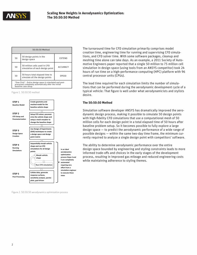
Figure 1. 50:50:50 method

Scaling New Heights in Aerodynamics Optimization: The 50:50:50 Method

2

The turnaround time for CFD simulation primarily comprises model creation time, engineering time for running and supervising CFD simula-tions, and CFD solver time. With some software packages, cleanup and meshing time alone can take days. As an example, a 2011 Society of Auto-motive Engineers paper reported that a single 50 million to 75 million cell simulation in design space (using tools from an ANSYS competitor) took 24 hours of run time on a high-performance computing (HPC) platform with 96 central processor units (CPUs).

The lead time required for each simulation limits the number of simula-tions that can be performed during the aerodynamic development cycle of a typical vehicle: That figure is well under what aerodynamicists and stylists desire.

The 50:50:50 Method

Simulation software developer ANSYS has dramatically improved the aero-dynamic design process, making it possible to simulate 50 design points with high-fidelity CFD simulations that use a computational mesh of 50 million cells for each design point in a total elapsed time of 50 hours after baseline problem setup. So it becomes possible to fully explore a large design space — to predict the aerodynamic performance of a wide range of possible designs — within the same two-day time frame, the minimum cur-rently required to analyze a single design point with competitors’ software.

The ability to determine aerodynamic performance over the entire design space bounded by engineering and styling constraints leads to more informed trade-offs and choices in the early stages of the development process, resulting in improved gas mileage and reduced engineering costs while maintaining adherence to styling themes.

50:50:50 Method

50

50

50

50 design points in the design space

50 million cells used in CFDsimulation of each design point

50 hours total elapsed time tosimulate all the design points

EXTEND

ACCURACY

SPEED

“One-Click” - Entire design space is simulated and post-processed completely automatically after the initialbaseline case setup

Figure 2. 50:50:50 aerodynamics optimization process

STEP 1 Baseline Model

STEP 2 CFD Setup and

STEP 3 Design Space

STEP 4 Running

STEP 5 Post Processing

shape and run CFD

points

Create geometry and meshed model for the baseline vehicle shape

Setup CFD solver; paramet-erize the vehicle shape and setup a mesh morpher to change the baseline shape

Use Design of Experiments (DOE) techniques to create a design space and design point matrix

Morph vehicle shape

Collate data, generate response surfaces,

plots, goal driven

In an ideal aerodynamics

process Steps 4 and 5 are completely automated requiring zero

to execute these steps

3

Meshing and Defining Computational Domain The new process begins like the old one with either a CAD model or 3-D scan of the vehicle. The model is imported into the surface mesher and a triangular surface mesh is created using the same method as the traditional approach. The surface mesh is then read into a volume mesher; a bound-ing box is created that marks the boundaries of the computational domain around the vehicle. A prism layer mesh with wedge-shaped elements is created on all surfaces of the vehicle to resolve the near-wall flow with the highest possible mesh resolution. The region between the top of the final prism layer and the bounding box is meshed with tetrahedral elements. Selective refinement boxes are used to gradually grow the element size with increasing distance from the vehicle surface. The use of high-fidelity meshes and physics ensures that the accuracy of the simulation is not compromised.

Defining Shape Parameters

At this point, the traditional method would solve the CFD model. Instead, the new 50:50:50 method uses a morpher that is integrated inside the ANSYS® Fluent® CFD solver to change the vehicle shape and the surround-ing computational mesh to solve a series of design points without having to manually create a new geometry and mesh. Engineers define a number of shape parameters that form the basis of the design space. For instance, in the example used in this paper, the boat tail angle is defined as the angle subtended by a line segment drawn from a vertical pivot-point axis passing through the top point of the rear wheel house to point B, which marks the beginning of the rear curvature, as shown in Figure 5.

Morpher Setup

Morpher setup is done as part of the CFD solver setup, since the morpher is integrated into the CFD solver. Figure 6 shows how the morpher is set up for varying the boat tail angle shape parameter. The encapsulation region, which is the area that will be altered by the morpher, is marked using a rectangular box. The surface selection tool in the morpher is used to select the surfaces that define the boat tail shape, and the rotation axis is speci-fied to complete the definition.

The morpher changes the locations of nodes in the computational mesh to change the shape of the vehicle surface and to match the surrounding surface and volume mesh to the new shape. The morpher uses a series of radial basis functions to produce a solution for the mesh movement using source point inputs and their displacements. The morpher incorporates a volume mesh smoother that preserves the volume mesh quality during morphing. The morpher operates in parallel with the CFD solver over a com-puter cluster, so in a matter of seconds it can morph meshes comprising 50 million nodes.

Scaling New Heights in Aerodynamics Optimization: The 50:50:50 Method

Figure 4. Computational domain

Figure 5. Definition of boat tail angle

Figure 3. Volvo XC60 development model used as test case

Figure 6. Setting up morpher for boat tail angle

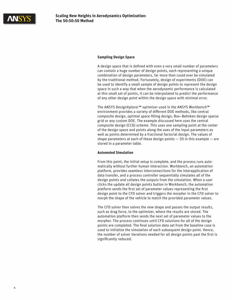
Sampling Design Space A design space that is defined with even a very small number of parameters can contain a huge number of design points, each representing a unique combination of design parameters, far more than could ever be simulated by the traditional method. Fortunately, design of experiments (DOE) can be used to identify a small sample of design points to represent the design space in such a way that when the aerodynamic performance is calculated at this small set of points, it can be interpolated to predict the performance of any other design point within the design space with minimal error.

The ANSYS DesignXplorer™ optimizer used in the ANSYS Workbench™ environment provides a variety of different DOE methods, like central composite design, optimal space-filling design, Box–Behnken design sparse grid or any custom DOE. The example discussed here uses the central composite design (CCD) scheme. This uses one sampling point at the center of the design space and points along the axes of the input parameters as well as points determined by a fractional factorial design. The values of shape parameters at each of these design points — 50 in this example — are stored in a parameter table.

Automated Simulation From this point, the initial setup is complete, and the process runs auto-matically without further human interaction. Workbench, an automation platform, provides seamless interconnections for the interapplication of data transfer, and a process controller sequentially simulates all of the design points and collates the outputs from the simulation. When a user clicks the update all design points button in Workbench, the automation platform sends the first set of parameter values representing the first design point to the CFD solver and triggers the morpher in the CFD solver to morph the shape of the vehicle to match the provided parameter values.

The CFD solver then solves the new shape and passes the output results, such as drag force, to the optimizer, where the results are stored. The automation platform then sends the next set of parameter values to the morpher. The process continues until CFD solutions for all of the design points are completed. The final solution data set from the baseline case is used to initialize the simulation of each subsequent design point. Hence, the number of solver iterations needed for all design points past the first is significantly reduced.

4

Scaling New Heights in Aerodynamics Optimization: The 50:50:50 Method

A unique feature of the ANSYS Fluent CFD solver is that it speeds up nearly linearly when the solver runs in distributed parallel mode over a number of computer cores. Scalability of the solver is shown in Figure 7. The number of cores used in the distributed parallel simulation comprises the hori-zontal axis and a performance measure, the inverse of the real time taken for running the simulation, makes up the vertical axis. Version 14.0 of the Fluent solver scales nearly linearly to well over 3,000 parallel cores. This near-perfect parallel scalability enables the Fluent solver to reduce the runtime of a large set of design points to mere hours.

Response Surface Data The optimizer then prepares a response surface from the collected data set of drag and other aerodynamic forces using one of several possible algorithms. For example, the nonparametric regression (NPR) algorithm is implemented in the optimizer as a metamodeling technique prescribed for predictably high nonlinear relation of the outputs with the inputs. NPR belongs to a general class of support vector method (SVM) techniques that use hyperplanes to separate data groups. The response surface enables stylists and engineers to visualize a vehicle’s aerodynamic performance over the entire design space and intuitively understand how the output variables, such as drag, are dependent on the chosen design parameters.

Sensitivity Analysis The response surface can be further processed to provide additional infor-mation that supports vehicle aerodynamic development efforts. Sensitivity analysis shows the sensitivity of output variables to input variables. For example, Figure 9 shows the local and global sensitivity of drag to four design parameters. Local sensitivity is the sensitivity of the output vari-able to the shape parameters at a particular design point. Global sensitivity represents the sensitivity of the response to the shape parameter averaged over the entire design space. The height of a column shows the relative effect of the corresponding shape parameter on drag. For example, increas-ing the long roof angle strongly increases drag, and decreasing the boat tail angle increases drag force.

5

Scaling New Heights in Aerodynamics Optimization: The 50:50:50 Method

Figure 8. Response surface data for test case

Figure 7. Parallel scalability of CFD solver

384 832 1280 1728 2176 2624 3072

Perfo

rman

ce

Number of Processor Cores

F1 140M AMD Magny-Cours

14.0.0

Ideal

Figure 9. Local and global sensitivity of drag to shape parameters

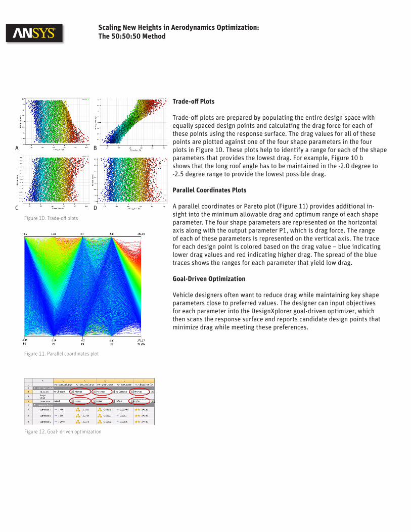
Trade-off Plots

Trade-off plots are prepared by populating the entire design space with equally spaced design points and calculating the drag force for each of these points using the response surface. The drag values for all of these points are plotted against one of the four shape parameters in the four plots in Figure 10. These plots help to identify a range for each of the shape parameters that provides the lowest drag. For example, Figure 10 b shows that the long roof angle has to be maintained in the -2.0 degree to -2.5 degree range to provide the lowest possible drag.

Parallel Coordinates Plots

A parallel coordinates or Pareto plot (Figure 11) provides additional in-sight into the minimum allowable drag and optimum range of each shape parameter. The four shape parameters are represented on the horizontal axis along with the output parameter P1, which is drag force. The range of each of these parameters is represented on the vertical axis. The trace for each design point is colored based on the drag value – blue indicating lower drag values and red indicating higher drag. The spread of the blue traces shows the ranges for each parameter that yield low drag.

Goal-Driven Optimization

Vehicle designers often want to reduce drag while maintaining key shape parameters close to preferred values. The designer can input objectives for each parameter into the DesignXplorer goal-driven optimizer, which then scans the response surface and reports candidate design points that minimize drag while meeting these preferences.

Scaling New Heights in Aerodynamics Optimization: The 50:50:50 Method

Figure 10. Trade-off plots

Figure 11. Parallel coordinates plot

Figure 12. Goal- driven optimization

A B

C D

ANSYS, Inc., is one of the world’s leading engineering simulation software provid-ers. Its technology has enabled customers to predict with accuracy that their product designs will thrive in the real world. The company offers a common platform of fully integrated multiphysics software tools designed to optimize product development processes for a wide range of industries. Applied to design concept, final-stage testing, validation and trouble-shooting existing designs, software from ANSYS can significantly speed design and development times, reduce costs, and provide insight and understanding into product and process performance. Visit www.ansys.com for more information.

Any and all ANSYS, Inc. brand, product, service and feature names, logos and slogans are registered trademarks or trademarks of ANSYS, Inc. or its subsidiaries in the United States or other countries. All other brand, product, service and feature names or trademarks are the property of their respective owners.

Toll Free U.S.A./Canada:1.866.267.9724Toll Free Mexico:001.866.267.9724Europe:44.870.010.4456eu.sales@ansys.com

ANSYS, Inc.Southpointe275 Technology DriveCanonsburg, PA 15317U.S.A.724.746.3304ansysinfo@ansys.com

© 2012 ANSYS, Inc. All Rights Reserved.

Figure 13. Velocity contours at y=0 cut plane for variousdesign points

Figure 14: Simulation run times for test case

Flow Field Output

Flow quantities such as pressure and velocity are automatically saved as the solver runs and can be displayed to gain insight into the effect of various shape parameters. For example, Figures 13 shows a view of the velocity flow field for four design points. Velocity contours on the vertical symmetry plane show the effect of the long roof angle parameter on wake size. Figure 13 c shows that the small wake of design point 19 helps to explain why it has such a low drag.

Results of Test Case

A recent design study using this method took approximately one week to prepare the CFD model and simulate the aerodynamic performance of 50 design points that covered four design parameters on the Volvo XC60 development vehicle model using the ANSYS Workbench automation plat-form, RBF Morph morpher and ANSYS Fluent CFD solver. As shown in Figure 14, the total run time for simulating 50 design points was 30.8 hours with 768 cores. Thus, with only one week of work, drag was reduced by 4 percent. The simulation output including response surfaces, sensitivity plots, trade-off plots and Pareto plots was given to stylists to help them understand and quantify the effect of styling choices on aerodynamics.

Conclusion

Today, most of the world’s major car and truck manufacturers use CFD simulation to evaluate aerodynamic drag one vehicle shape at a time. The 50:50:50 method enables car and truck makers to simulate many hundreds of vehicle shape variants in a matter of days with high-fidelity, detailed CFD simulations. By simulating so many variants, aerodynamics engineers can give detailed guidance to stylists about the specific effects on drag of numerous shape parameters — such as boat tail and front spoiler angles — in the form of response surfaces, Pareto plots, trade-off charts, etc. Armed with such information, stylists and aerodynamicists can then make great headway into reducing drag, performing goal-driven optimization, and identifying vehicle shapes that yield the least drag while adhering to styling themes and requirements.

Scaling New Heights in Aerodynamics Optimization: The 50:50:50 Method

A

C

B

D