Test Data Generation with a Kalman Filter-Based

Adaptive Genetic Algorithm

Aldeida Aletia, Lars Grunskeb

aFaculty of Information Technology, Monash Universityemail: aldeida.aleti@monash.edu

bInstitute of Software Technology, University of Stuttgartemail: lars.grunske@informatik.uni-stuttgart.de

Abstract

Software testing is a crucial part of software development. It enables quality assurance,such as correctness, completeness and high reliability of the software systems. Currentstate-of-the-art software testing techniques employ search-based optimisation methods,such as genetic algorithms to handle the difficult and laborious task of test data generation.Despite their general applicability, genetic algorithms have to be parameterised in orderto produce results of high quality. Different parameter values may be optimal for differentproblems and even different problem instances. In this work, we introduce a new approachfor generating test data, based on adaptive optimisation. The adaptive optimisationframework uses feedback from the optimisation process to adjust parameter values of agenetic algorithm during the search. Our approach is compared to a state of the arttest data optimisation algorithm that does not adapt parameter values online, and arepresentative adaptive optimisation algorithm, outperforming both methods in a widerange of problems.

Keywords: test data generation, optimisation, genetic algorithm, adaptive parametercontrol

1. Introduction

Search-based optimisation methods, such as genetic algorithms, ant colony optimisa-tion and simulated annealing have successfully been applied in solving a wide range ofsoftware testing problems [41, 30, 2, 31, 40, 21]. The commonality of these approaches isthat they aim at optimising the quality of a given test data set. Quality could be measuredwith respect to certain coverage criteria, eg. branch, statement, and method coverage forsource code, or metrics such as transition coverage for model-based testing. Beside thesefunction-oriented approaches, a variety of methods focus on non-functional aspects of testdata optimisation, such as searching for input situations that break memory or storagerequirements, automatic detection of memory leaks, stress testing and security testing. Asystematic literature review of search-based testing for non-functional system propertiesby Afzal et al. [1] presents a comprehensive overview of these methods.

Genetic algorithms (GAs) are among the most frequently applied search-based op-timisation method in test data generation [4]. GAs provide approximate results whereexact approaches cannot be devised and optimal solutions are hard to find. They can

Preprint submitted to Journal of Systems and Software October 4, 2014

be used by practitioners as a ‘black box’, without mastering advanced theory, whereasmore sophisticated exact approaches are tailored to the specific mathematical structureof the problem at hand, and can become completely inapplicable if small aspects of theproblem change. Another advantage of GAs compared to traditional methods, such asgradient descent-based algorithms is the stochastic element which helps them get out oflocal optima.

In recent years, it has been acknowledged that the performance of GAs depend on thenumerous parameters, such as crossover rate, mutation rate and population size [19, 17, 3].Algorithm parameters determine how the search space is explored. They are responsiblefor the flexibility and efficiency of the search procedure, and when configured appropri-ately, produce high-quality results regardless of the search space difficulty. Because of theinfluence of parameter values on algorithm performance, poor algorithm parameterisationhinders the discovery of solutions with high quality [39, 19, 17]. It has been acknowledgedthat parameters required for optimal algorithm performance are not only domain-specific,but also have to be chosen based on the problem instance at hand [18].

The configuration of the algorithm is usually the responsibility of the practitioner,who often is not an expert in search-based algorithms. General guidelines for successfulparameter values give different recommendations: e.g. De Jong [14] recommends using 0.6for crossover rate, Grefenstette [27] suggests 0.95, whereas Schaffer et al. [48] recommendsany value in the range [0.75, 0.95]. These general guidelines conflict with each other,because each one reports the best parameter configuration of a GA for a particular classof problems. For a newly arising problem, the search space is typically unknown, hence itis hard to formulate any general principles about algorithm parameter configurations foruniversal applicability [42]. In these circumstances, algorithm parameterisation presentsitself as an optimisation problem in its own right [19]. To save time, practitioners tend toconfigure the GA based on a few preliminary runs, where different parameter values aretried in an attempt to fine-tune the algorithm to a particular problem [19]. Dependingon the number of parameters and their possible values, investigative trials for parameteroptimisations can themselves be attempts to solve a combinatorially complex problem.Even if parameters are tuned to their optimal values, there is no guarantee that theperformance of the algorithm will be optimal throughout the optimisation process. In fact,it has been empirically and theoretically demonstrated that different parameter settingsare required for different stages of the optimisation process [9, 8, 52, 50, 32, 11, 55]. Thismeans that tuning parameter values before the optimisation process does not guaranteeoptimal GA performance. This problem has been tackled by many researchers in theoptimisation community, who propose to set GA parameter values during the run usingfeedback from the search, known as adaptive parameter control [17, 25, 22, 12, 13, 33,34, 36, 38, 49, 56]. The intuitive motivation comes from the way the optimisation processunfolds from a more diffused global search, requiring parameter values responsible forthe exploration of unseen areas of the search space, to a more focused local optimisationprocess, requiring parameter values which help with the convergence of the algorithm.

In essence, adaptive parameter control methods monitor the behaviour of a GA run,and use the performance of the algorithm to adapt parameter values, such that successfulparameter values are propagated to the next generation. The majority of adaptive param-eter control methods found in the literature belong to the class of probability matching

2

techniques [12, 13, 33, 34, 36], in which the probability of applying a parameter valueis proportional to the quality of that parameter value. The earliest approaches [34, 33]lacked the exploration of parameter values if the feedback from the algorithm was notin their favour in the initial phases of the process. In later work, a minimum selectionprobability was introduced [34], to ensure that under-performing parameter values didnot disappear during the optimisation, in case they were beneficial in the later stages ofthe search. One of the more recent and mature examples of probability matching is thework by Igel and Kreutz [34], where the selection probability for each parameter valueincorporates a minimum probability of selection.

These adaptive parameter control methods assume that the improvement in the qualityof the solutions is directly related to the use of certain parameter values. However, GAs arestochastic systems that may produce different results for the same parameter values [16].Ideally, the randomness induced by the stochastic behaviour of GAs should be taken careof by the parameter control strategy. To address this issue, we introduce an adaptivegenetic algorithm, which adjusts algorithm parameters during the optimisation processusing a Kalman filter. The Kalman filter-based genetic algorithm (KFGA) redefinesparameter values repeatedly based on a learning process that receives its feedback fromthe optimisation algorithm. The Kalman filter is employed to reduce the noise factorfrom the stochastic behaviour of GAs when identifying the effect of parameter values onthe performance of the algorithm. KFGA outperforms a GA with pre-tuned parametervalues and the probability matching technique by Igel and Kreutz [34] when solving theproblem of test data generation. The proposed methods consistently finds test suites withbetter branch coverage than the state-of-the-art, as shown by the experiments performedon a set of open-source problem instances.

2. Test Data Generation

Software testing is used to estimate the quality of a software system. Quality mayrefer to functional attributes, which describe how the system should behave, or non-functional requirements as defined in ‘IEEE International Standard 1471 2000 — Sys-tems and software engineering — Recommended practice for architectural description ofsoftware-intensive systems’ [35], such as reliability, efficiency, portability, maintainability,compatibility and usability.

A software test consists of two main components, an input to the executable programand a definition of the expected outcome. In software testing, the aim is to find thesmallest number of test cases that expose as many scenarios as possible in which thesystem may fail. It is important that the generated test inputs cover as many lines ofcode as possible. However, since it is usually the task of a human tester to specify theexpected outcome, it is also essential to keep the number of test cases as small as possibleto make this task feasible.

Due to the time-consuming nature and computational load of this task, optimisationtechniques, such as genetic algorithms have been used to automate the process of testcase generation [23, 58, 51, 54, 26]. A common approach is to use coverage criteria, suchas branch coverage [23] to measure the quality of generated test cases and guide the opti-misation process towards the optimal solution(s) that maximise or minimise the criteria.Coverage criteria are a set of coverage goals, which are usually optimised separately [29].

3

However, it is often the case that testing goals conflict with each other, hence should beoptimised simultaneously. EvoSuite [23] addresses the problem of conflicting test goalsby evolving test cases in a test suite simultaneously with a genetic algorithm, known aswhole test suite generation. We use the EvoSuite framework1 to model the optimisationproblem of test suite generation, and extend it to incorporate adaptive optimisation whichadjusts the parameter values of the GA during the optimisation process.

3. Optimisation Model for Test Data Generation

GAs evolve a population of solutions using the genetic operators: mutation, crossover,selection, and replacement procedure. The aim is to optimise some quality function(s)by searching the space of potential solutions. GAs start the optimisation process byrandomly generating a set of solutions. In certain cases, this initial set of solutions iscreated by applying heuristic rules (e.g. greedy algorithm), or obtained using expertknowledge. Usually, the genetic operators are applied based on predefined rates, such asfor crossover or mutation. These operators are employed to create the new solutions bychanging excising solutions that are selected according to the selection procedure. Thenew candidate solutions are added to the pool of population. Finally, the set of solutionsthat will survive to the next generation are selected using the replacement procedure,which removes as many individuals as required to maintain the prescribed populationsize.

For test data generation we employ EvoSuite [23], which evolves test suites using aGA with the aim of covering all test goals while minimising the total size of the suite. Tomeasure the quality of a solution, we use branch coverage as an objective function. Theaim is to cover as many control structures, such as if and while statements as possible,by evaluating the logical predicates that result in both true and false. In order for allbranches to be covered, each predicate should be executed at least twice, resulting in trueand false values. In EvoSuite, the branch distance d(b, T ) for each branch b in test suiteT is defined as

d(b, T ) =

0 if the branch has been covered,dmin(b, T ) if the predicate has been executed at least twice,1 otherwise.

(1)

The distance dmin(b, T ) is 0 if at least one of the branches has been covered, and > 0otherwise. The fitness function that is minimised by EvoSuite and used in the experimentsin Section 6 is formally defined as

f(T ) = |M | − |MT |+∑b∈B

d(b, T ), (2)

where |M | is the total number of methods, |MT | is the number of executed methods in testsuite T and B is the set of branches in the program. The optimisation process in EvoSuitestarts with a set of solutions, which are uniformly, randomly generated. Formally, let t

1EvoSuite can be downloaded from http://www.evosuite.org.

4

denote a test case, composed of a sequence of statements t = 〈s1, s2, ..., sl〉 of length l.A statement si can be a constructor, a field, a primitive, a method or an assignment. Asolution is defined as a collection of T = {t1, t2, ..., tn} of test cases. The test suite shouldnot only cover as many branches as possible, but also be the shortest possible. Hence, anoptimal solution T ∗ is a test suite that covers all possible branches, but at the same timehas the smallest possible number of statements. The sum of the lengths of all test casesin a test suite defines its length, i.e.

|T | =n∑i=1

|ti|. (3)

Since the number of test cases in a test suite and the number of statements in a testcase may vary, the solution representation is of a variable size. The solutions are evolvedin iterations until a stopping criterion is achieved. The new generations of solutions arecreated with the help of four genetic operators: the crossover operator, the mutationoperator, the selection operator and the replacement operator. The crossover operatorcreates two new solutions T ′1 and T ′2 by combining test cases from two pre-existing testsuites T1 and T2. A parameter α, which is randomly selected in the range [0, 1] indicateshow the solutions are combined: the first new solution T ′1 receives dα|T1|e test cases fromT1 and the rest from T2, whereas the new second solution is composed of the first α|T2|test cases from the second parent solutions and b(1 − α)|T1|c test cases from the secondparent.

The mutation operator is applied after the crossover operator. There are two differenttypes of mutations that can occur: at a test suite level and at a test case level. Testsuites are mutated by changing each of the test cases with a probability 1/n, where n isthe number of test cases in the test suite. At the same time, new test cases are added tothe test suite with a probability σ. Mutation of test cases is performed by either adding,changing or removing statements from a test case with a probability 1/l, where l is thenumber of statements in a test case.

A rank-based selection procedure is employed to select the parent solutions that willundergo recombination and mutation procedures [57]. Solutions are ranked based on thefitness function defined in eq. 2. When there is a tie between solutions, shorter testsuites are assigned better ranks. As a result, solutions with better branch coverage andshorter length have a higher chance of projecting their ‘genes’ to the next generation.Similar to the original studies with EvoSuite, an elitist strategy is used as a replacementprocedure [23]. The elitist strategy selects the best solutions to create the next generation.

4. Adjusting Parameters of Genetic Algorithms

Genetic algorithms (GAs) have successfully been applied to Whole Test Suite Gen-eration [23] and many other optimisation problems in Software Engineering [46, 28, 5].The performance of GAs is affected by the configuration of its parameter values, such ascrossover rate, mutation rate and population size [10, 20, 15, 6]. Parameter values can beconfigured in two different ways: by tuning their values before the optimisation process,or by dynamically adjusting parameter assignments during the run. The later is referredto as parameter control, and is more effective than parameter tuning, since different algo-

5

rithm configurations may be optimal at different stages of the search [10, 20, 15, 6]. Aninvestigation on the benefit of tuning parameter values for solving software engineeringproblems showed that tuned parameter values do not necessarily produce better algorithmperformance compared to default parameter values [7].

Parameter control methods can be classified into three groups: deterministic, self-adaptive and adaptive. Deterministic parameter control changes parameter values basedon a predefined schedule composed of intervals with preassigned parameter values, e.g.decreasing mutation rate by a certain amount every iteration. Using a predefined sched-ule is likely to lead to suboptimal values for some problems or instances, since smallerproblems may require shorter intervals for the schedule, as the search progress will befaster when the problem complexity is lower.

Alternatively, the search for optimal parameters can be integrated into the optimi-sation process itself — usually by encoding parameter settings into the genotype of thesolution to evolve [10, 20, 15], known as self-adaptive parameter control. Extending thesolution size to include the parameter space obviously increases the search space andmakes the search process more time-consuming [17]. The approach proposed in this workfalls into the category of adaptive parameter control, in which feedback from the optimi-sation process is collected and used to evaluate the effect of parameter value choices andadjust the parameter values over the iterations.

Adaptive parameter control does not use a predefined schedule and does not extendthe solution size, which makes it a more effective way for adjusting parameter values. Fur-thermore, unlike self-adaptive methods, adaptive strategies use feedback from the searchto adjust parameter values based on their ability to create high-quality solutions. Thegenetic operators, and other elements of a GA that are involved in the optimisation pro-cess, such as the probabilities of applying the genetic operators, the size of the population,and the number of new solutions produced at every iteration are the parameters of thealgorithm that can be adapted by the parameter control method.

Every iteration, the solutions created are evaluated using the objective function, which,in our case, is the branch coverage. The output from the evaluation process is used toassess the effect of the parameter values on the performance of the optimisation algorithm.The approximated effect is employed for a projection of parameter values performingwell to the next iterations, based on certain rules, such as the average effect over anumber of iterations, instantaneous effect, or the total usage frequency of parametervalues. The quality values assigned to the algorithm parameters are used to select thenext parameter values, which are employed to create the next generation of solution(s).The selection mechanism configures the components of a GA (variation, selection andreplacement operators). The main challenge faced at this step is the trade-off that hasto be made between the choice of current best configuration(s) and the search for newoptimal settings.

5. Effect Assessment of Parameter Values using the Kalman Filter

Formally, given a set {υ1, ..., υn} of n algorithm parameters, where each parameter υihas {υi1, ..., υim} values that can be discrete numbers or intervals of continuous numbers,parameter control derives the optimal next value υij to optimise the effect of υi on the

6

performance of the algorithm [3]. As an example, when the mutation rate υ1 is dynami-cally adjusted by considering 4 intervals (m = 4), υ12 stands for a mutation rate sampledfrom the second interval. In the discrete case of optimising the type of mutation operatorυ2, υ22 could represent the single-point mutation operator.

Adaptive parameter control methods keep a vector of probabilities denoted as P ={p(υ11), p(υ12), ..., p(υ1m1), ..., p(υnmn)}, which represents the selection probability for eachparameter value υij. At each time step, the jth value of the ith parameter is selected withprobability p(υij). Its effect on the performance of the algorithm is denoted as e(υij).The main goal of adaptive parameter control is to adapt the vector of probabilities P tomaximize the expected value of the cumulative effect E[E ] =

∑ni=1 e(υij) [3]. The adaptive

parameter control employed in this work adjusts parameter values as the optimisationprocess progresses, using feedback from the search space. Due to the stochastic natureof GAs, the discovery of high-quality solutions may not always be related to algorithmparameters. Instead, the performance of the algorithm is highly susceptible to noise anderror, involving random effects of parameter values.

To reduce the noise factor from the stochastic behaviour of GAs, we employ theKalman filter [37]. The Kalman filter uses a series of measurements observed over timethat usually contain noise, and produces a statistically optimal estimate of unknownvariables. The algorithm has two main phases: first, it uses previous measurementsto predict the current behaviour of parameter values, along with their uncertainties andtaking into account noise. In the second phase, once the outcome of the next measurementis observed, which usually contains noise, the estimates are updated using a weightedaverage, with highly certain estimates being given more weight. As a result, Kalmanfilter produces reliable estimates of the true performance of parameter values.

5.1. Kalman Filter Model

The effect of a parameter value on the performance of the optimisation algorithmis approximated as the fitness change of the solution created by that parameter valuecompared to the parent solution. More specifically, if a parameter value υij creates asolution s

υijk by modifying a parent solution sk, the effect of υij on the performance of the

optimisation algorithm is calculated as:

e(υij) = f(sυijk )− f(sk), (4)

where f(sυijk ) and f(sk) are the fitnesses of the child and parent solutions respectively.

The observed effect e(υij) is stochastic, susceptible to noise and error. This is due to theprobabilistic behaviour of GAs, which produce different results for the same parametervalues. Hence, instead of using the fitness change to describe the effect of parameter values(eq. 4), the parameter control strategy investigated in this work performs a stochasticestimation of the effect parameter values. To this end, we employ the Kalman filter [37].

Kalman filter has successfully been used for tracking and data prediction problems.It is implemented as a predictor-corrector estimator, which minimises the estimated errorcovariance. The relationship between the parameter value effect at time t and the effectat the previous iteration t − 1 is represented by an n × n matrix A. In this paper, weassume A is constant over time. The optional control input u ∈ Rl is denoted using then × 1 matrix B. Finally, an m × n matrix H relates the state of the system (parameter

7

effect) to measurement e′t. The filter estimates the state e ∈ Rn of a process (effect of aparameter value) governed by a linear stochastic difference equation modelled as follows:

et = Aet−1 +But + wt−1, (5)

In our application of the Kalman filter, B is a zero matrix, since we do not have a controlinput. Hence, eq. 6 can be simplified to

et = Aet−1 + wt−1, (6)

with a measured effect e′t ∈ Rm defined as

e′t = Het + vt. (7)

The random variables wt−1 and vt represent the process and measurement noise, as-sumed to be normally distributed and independent of each other. If the noise is notnormally distributed, the Kalman filter tries to converge to correct estimations.

The Kalman filter model has previously been used to deal with aspects of uncertainty inGAs. Stroud [53] used the Kalman formulation for stochastic problems, where the fitnessfunction is affected by nonstationary noisy environments. Other works have employed theKalman model in the context of particle swarm optimisation, such as the Kalman Swarmalgorithm [43], which uses the filter to update the position of particles. In this work, weapply the Kalman model for estimating the effect of parameter values on the performanceof the algorithm, which to the best of our knowledge has not been previously investigated.

5.2. Kalman Filter Algorithm

The feedback control loop of the Kalman filter has two distinct sets of equations: timeupdate equations used in prediction and measurement update equations, necessary forcorrection. The time update equations are

e−t = Aet−1 (8)

which projects the state ahead, and

P−t = APt−1AT +Q, (9)

which projects the error covariance P ahead. Matrices A and B are the same as in eq. 6,whereas Q is the process noise covariance matrix. The update equations are

Kt = P−t HT (HP−t H

T +R)−1 (10)

et = e−t +Kt(e′t −He−t ) (11)

Pt = (I −KtH)P−t . (12)

Equation 10 calculates the Kalman gain Kt at time t, where R is the measured errorcovariance. As R approaches zero, the gain K weights the residual more heavily. Equa-tion 11 computes the a posteriori state et from the measurement e−t . Finally, equation 12

8

estimates the a posteriori covariance matrix Pt. In the next time step, the a posteri-ori estimates are used to predict the new a priori estimates. This process is performedrecursively.

Algorithm 1 Kalman filter-based adaptive genetic algorithm (KFGA).

1: procedure KFGA2: input: f - fitness function3: µ - population size4: SC - stopping criterion5: λ - number of children per generation6: m, mr - mutation operator and mutation rate7: c, cr - crossover operator and crossover rate8: output: st - evolved set of solutions9: s0 ← GenerateRandomSolutions(µ)

10: t = 011: while !SC do12: Evaluate(f, st)13: parentst = SelectParents(s, st)14: childrent =Evolve(parentst, λ, m, mr, c, cr)15: st+1 = Replace(childrent, st, r, µ)16: AdaptiveParameterControl(λ, m, mr, c, cr, t)17: t = t+ 118: end while19: return st20: end procedure

21: procedure AdaptiveParameterControl22: input: υi, ..., υn - set of parameters to be adapted23: t - time step24: for all parameters υi, i ∈ n do25: for all parameter values υij , j ∈ m do26: et(υij) = KalmanFilter(υij , t)27: end for28: υij = ParameterValueSelection(et(υi1), ..., et(υim))29: end for30: end procedure

31: procedure KalmanFilter(υij , t)32: input: υij - parameter value33: t - time step34: output: et(υij) - effect of parameter value35: e−t (υij) = Aet−1(υij) +Buk36: P−t = APt−1A

T +Q37: Kt = P−t H

T (HP−t HT +R)−1

38: Pt = (I −KtH)P−t39: et(υij) = e−t (υij) +Kt(e

′t(υij)−He−t (υij))

40: return et(υij)41: end procedure

9

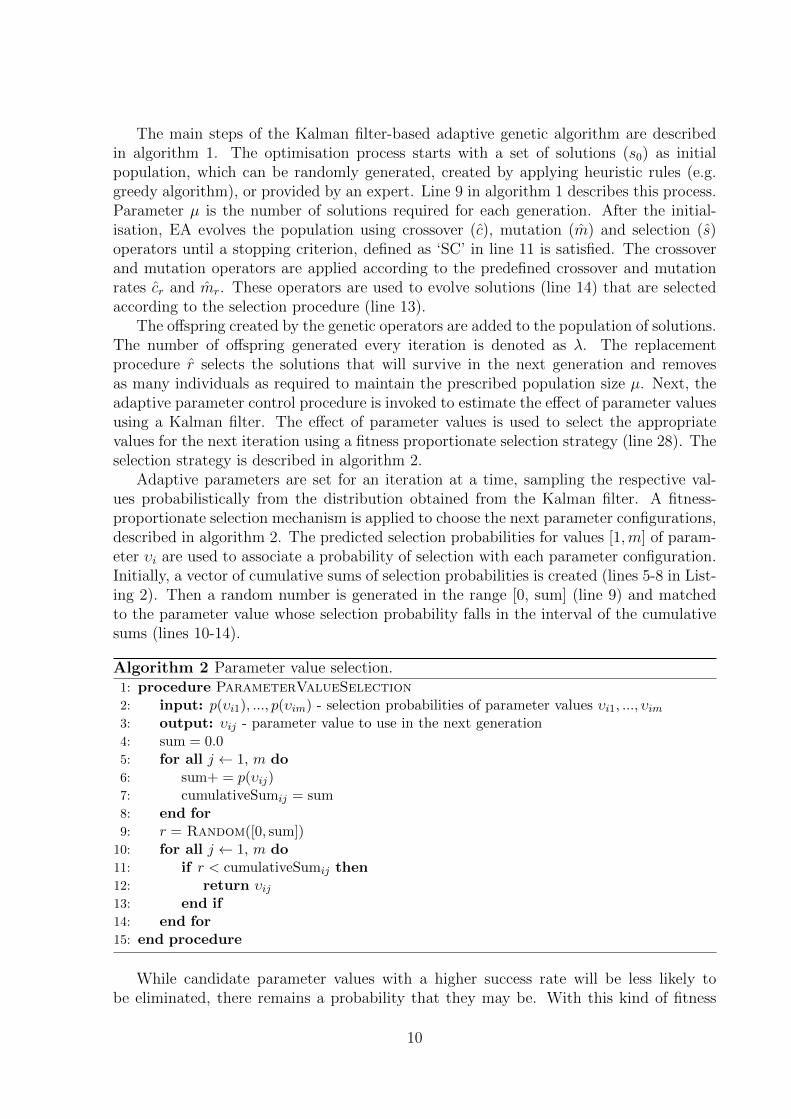
The main steps of the Kalman filter-based adaptive genetic algorithm are describedin algorithm 1. The optimisation process starts with a set of solutions (s0) as initialpopulation, which can be randomly generated, created by applying heuristic rules (e.g.greedy algorithm), or provided by an expert. Line 9 in algorithm 1 describes this process.Parameter µ is the number of solutions required for each generation. After the initial-isation, EA evolves the population using crossover (c), mutation (m) and selection (s)operators until a stopping criterion, defined as ‘SC’ in line 11 is satisfied. The crossoverand mutation operators are applied according to the predefined crossover and mutationrates cr and mr. These operators are used to evolve solutions (line 14) that are selectedaccording to the selection procedure (line 13).

The offspring created by the genetic operators are added to the population of solutions.The number of offspring generated every iteration is denoted as λ. The replacementprocedure r selects the solutions that will survive in the next generation and removesas many individuals as required to maintain the prescribed population size µ. Next, theadaptive parameter control procedure is invoked to estimate the effect of parameter valuesusing a Kalman filter. The effect of parameter values is used to select the appropriatevalues for the next iteration using a fitness proportionate selection strategy (line 28). Theselection strategy is described in algorithm 2.

Adaptive parameters are set for an iteration at a time, sampling the respective val-ues probabilistically from the distribution obtained from the Kalman filter. A fitness-proportionate selection mechanism is applied to choose the next parameter configurations,described in algorithm 2. The predicted selection probabilities for values [1,m] of param-eter υi are used to associate a probability of selection with each parameter configuration.Initially, a vector of cumulative sums of selection probabilities is created (lines 5-8 in List-ing 2). Then a random number is generated in the range [0, sum] (line 9) and matchedto the parameter value whose selection probability falls in the interval of the cumulativesums (lines 10-14).

Algorithm 2 Parameter value selection.1: procedure ParameterValueSelection2: input: p(υi1), ..., p(υim) - selection probabilities of parameter values υi1, ..., υim3: output: υij - parameter value to use in the next generation4: sum = 0.05: for all j ← 1, m do6: sum+ = p(υij)7: cumulativeSumij = sum8: end for9: r = Random([0, sum])

10: for all j ← 1, m do11: if r < cumulativeSumij then12: return υij13: end if14: end for15: end procedure

While candidate parameter values with a higher success rate will be less likely tobe eliminated, there remains a probability that they may be. With this kind of fitness

10

proportionate selection, there is a chance that some weaker solutions may survive theselection process; this is an advantage, as though a parameter value may be not as suc-cessful, it may include some component which could prove useful in the following stagesof the search.

6. Experimental Evaluation

The new adaptive control method is applied to adjust the mutation and crossoverrate of a GA during the optimisation process2. The experiments were conducted usingEvoSuite [23], described in Section 3. The Kalman filter-based adaptive parameter controlwas compared against pre-tuned parameter settings and probability matching technique(PM) [34]. The three optimisation schemes were used to optimise the same set of probleminstances. A fixed number of computations was used as a stopping criterion. The probleminstances, experimental settings and results are described in the following sections.

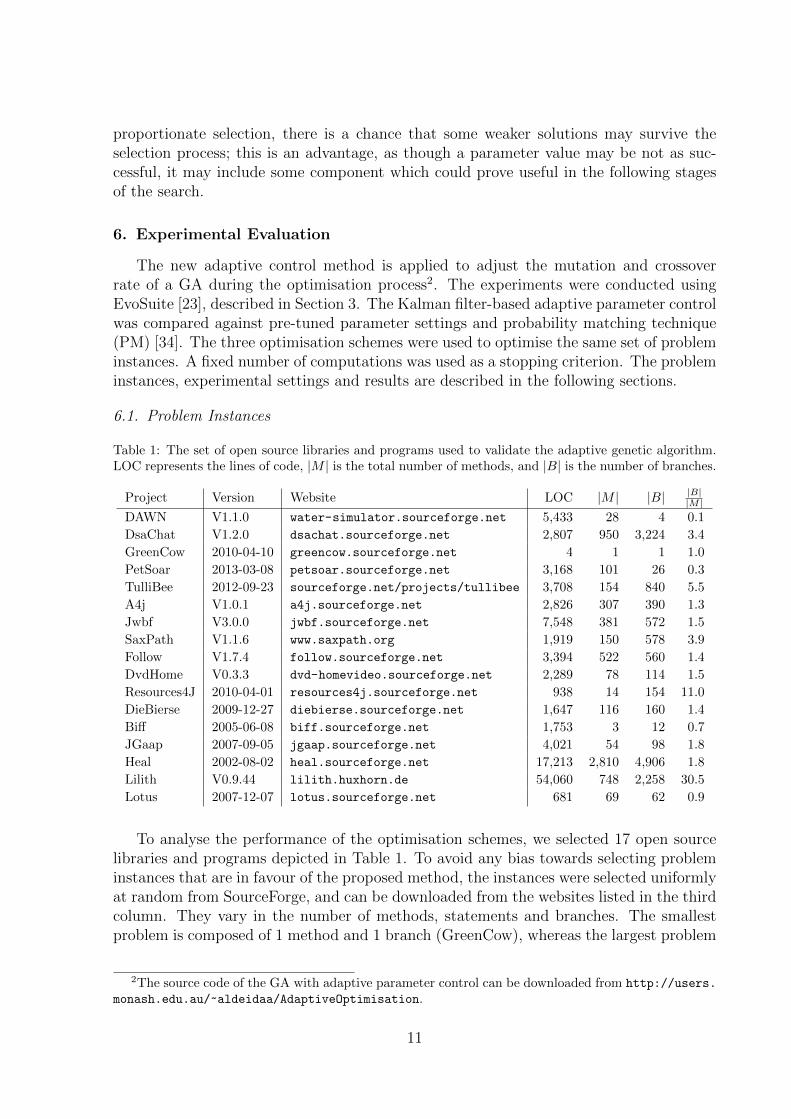
6.1. Problem Instances

Table 1: The set of open source libraries and programs used to validate the adaptive genetic algorithm.LOC represents the lines of code, |M | is the total number of methods, and |B| is the number of branches.

Project Version Website LOC |M | |B| |B||M |

DAWN V1.1.0 water-simulator.sourceforge.net 5,433 28 4 0.1

DsaChat V1.2.0 dsachat.sourceforge.net 2,807 950 3,224 3.4

GreenCow 2010-04-10 greencow.sourceforge.net 4 1 1 1.0

PetSoar 2013-03-08 petsoar.sourceforge.net 3,168 101 26 0.3

TulliBee 2012-09-23 sourceforge.net/projects/tullibee 3,708 154 840 5.5

A4j V1.0.1 a4j.sourceforge.net 2,826 307 390 1.3

Jwbf V3.0.0 jwbf.sourceforge.net 7,548 381 572 1.5

SaxPath V1.1.6 www.saxpath.org 1,919 150 578 3.9

Follow V1.7.4 follow.sourceforge.net 3,394 522 560 1.4

DvdHome V0.3.3 dvd-homevideo.sourceforge.net 2,289 78 114 1.5

Resources4J 2010-04-01 resources4j.sourceforge.net 938 14 154 11.0

DieBierse 2009-12-27 diebierse.sourceforge.net 1,647 116 160 1.4

Biff 2005-06-08 biff.sourceforge.net 1,753 3 12 0.7

JGaap 2007-09-05 jgaap.sourceforge.net 4,021 54 98 1.8

Heal 2002-08-02 heal.sourceforge.net 17,213 2,810 4,906 1.8

Lilith V0.9.44 lilith.huxhorn.de 54,060 748 2,258 30.5

Lotus 2007-12-07 lotus.sourceforge.net 681 69 62 0.9

To analyse the performance of the optimisation schemes, we selected 17 open sourcelibraries and programs depicted in Table 1. To avoid any bias towards selecting probleminstances that are in favour of the proposed method, the instances were selected uniformlyat random from SourceForge, and can be downloaded from the websites listed in the thirdcolumn. They vary in the number of methods, statements and branches. The smallestproblem is composed of 1 method and 1 branch (GreenCow), whereas the largest problem

2The source code of the GA with adaptive parameter control can be downloaded from http://users.

monash.edu.au/~aldeidaa/AdaptiveOptimisation.

11

has 748 methods and 2258 branches (Lilith). The second column in Table 1 shows theversion or latest update of the programs used in the experiments.

Branch coverage is used as an indicator of the performance of the optimisation algo-rithm. Branch coverage evaluates whether Boolean expressions tested in control struc-tures (if-statement and while-statement) evaluate to both true and false. The numberof branches and their ratio to the number of methods in a problem instance affects thismetric, and is an indication of problem difficulty. Hence, we have selected a wide rangeof problems with different number of branches and branch/method ratios, as depicted inTable 1.

6.2. Experimental Settings

The crossover and mutation operators and their rates are probably the most prominentcontrol parameters to optimise in genetic algorithms [9]. Hence, for the benefit of theexperiments, the crossover and mutation rates were varied, with different value intervalsto sample from. Preliminary trials have shown that a cardinality of four intervals inthe range {[0.7, 0.775), [0.775, 0.85), [0.85, 0.925), [0.925, 1.0)} produced the best resultsamong several cardinalities with even spreads between 0.7 and 1 for crossover rate, andfour intervals in the range [0.001, 0.3] for mutation rate.

The parameter values for the pre-tuned GA are based on recommendation from Fraserand Arcuri [23], many of which are ‘best practice’. The crossover rate is set to 0.75, therate of inserting a new test case is 0.1, whereas the rate for inserting a new statement is0.5.

6.3. Benchmark Methods

The proposed method is compared against the probability matching technique (PM),which is one of the most prominent techniques for adjusting GA parameters [34]. PMcalculates the selection probability for each parameter value at time step t as

pt(υij) =

{w/(

∑mr=1 qt(υir))

∑t−1r=t−τ qr(υij) + (1− w)pt−1(υij) if

∑mr=1 q(υis) > 0

wm

+ (1− w)pt−1(υij) otherwise,(13)

where m is the number of possible values for parameter υi, τ is the time window consideredto approximate the quality of a parameter value, and w ∈ (0, 1] is the weight given toeach parameter value.

Igel and Kreutz [34] introduce a minimum selection probability pmin for each parametervalue, to ensure that under-performing parameter values do not disappear during theoptimisation, since they may be beneficial in the later stages of the search. The selectionprobability for each parameter value is calculated using eq. 14.

p′t(υij) = pmin + (1−mpmin)pt(υij)∑mr=1 pt(υir)

(14)

Dividing the selection probability by the sum of selection probabilities of all possibleparameter values normalises the values in the interval [0,1].

12

6.4. Comparative Measure

To obtain a fair comparison, the generally accepted approach is the Mean of SolutionsQuality (MSQ), which allows the same number of function evaluations for each trial [47].Therefore, for the current comparison, all trials were repeated 30 times for each optimi-sation scheme, for 1, 000, 000 function evaluations, i.e. maximum number of statementscreated. These values were decided after running the algorithm once for every problemand choosing the value where the quality of the solutions seemed to not improve any fur-ther. Nevertheless, there are indications that all algorithms still make small but steadyimprovements after these numbers of evaluations. MSQ considers the stochastic natureof GAs, which leads to different results for different runs, by expressing the performancemeasure as the mean of the final quality of the solutions over a number of independentruns. Altogether 30 independent runs are performed per optimisation scheme and testproblem in order to restrict the influence of random effects. A different initial popula-tion is randomly created each time, and for each test problem all GAs operate on thesame 30 initial populations. The MSQ can always be used to measure the performanceof stochastic optimisers, since it does not require the optimal solutions. In order to checkfor a statistical difference in the outperformance of the optimisation schemes, results arevalidated using the Kolmogorov-Smirnov (KS) non-parametric test [45].

6.5. Analysis of Results

The results of the experiments are shown in Table 2, 3 and 4. For each probleminstance and optimisation scheme, we have recorded the test coverage as the percentageof total goals covered, branch coverage as the percentage of branches covered, and the testsuite length. Total goals represent method and branch coverage. The most importantindicator of the performance of the optimisation algorithm is the branch coverage, since itis the primary objective considered during the optimisation process. In the case of branchand goal coverage, higher mean values indicate better performance, whereas for test suitelength lower values are more desirable.

Table 3 shows the mean, standard deviation and KS test values of branch coverageover the 30 runs of the optimisation schemes and problems instances. It can be observedthat the Kalman filter-based Genetic algorithm (KFGA) has outperformed the standardgenetic algorithm (SGA) and the GA with probability matching parameter control (PM)in the majority of the problem instances with respect to branch coverage. The differencein results is more evident for larger problems, such as Heal (2810 methods, and 4906branches), TulliBee (154 methods, and 840 branches), and DsaChat (950 methods, and3224 branches).

In the case of GeenCow and Biff, all optimisation schemes find test suites with 100%branch coverage. GeenCow is a very small problem, with 1 method and 1 branch. Biff, onthe other hand, is a slightly bigger problem, with 3 methods and 2 branches. However, it isstill relatively small compared to the other problems considered. A 100% branch coverageensures that all branches in terms of control flow are executed at least once. A highbranch coverage helps ensure correct functionality. In the larger problem instances, thethree optimisation schemes (KFGA, SGA and PM) do not achieve 100% branch coverage.The larger the problem, the lower the branch coverage is, with DvdHomevideo havingthe smallest value for branch coverage. Although, this assertion is not always true. For

13

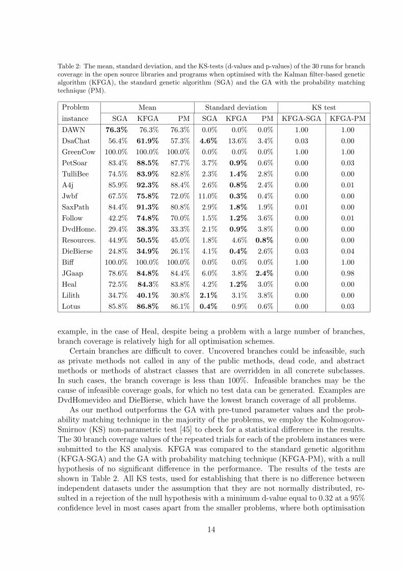
Table 2: The mean, standard deviation, and the KS-tests (d-values and p-values) of the 30 runs for branchcoverage in the open source libraries and programs when optimised with the Kalman filter-based geneticalgorithm (KFGA), the standard genetic algorithm (SGA) and the GA with the probability matchingtechnique (PM).

Problem Mean Standard deviation KS test

instance SGA KFGA PM SGA KFGA PM KFGA-SGA KFGA-PM

DAWN 76.3% 76.3% 76.3% 0.0% 0.0% 0.0% 1.00 1.00

DsaChat 56.4% 61.9% 57.3% 4.6% 13.6% 3.4% 0.03 0.00

GreenCow 100.0% 100.0% 100.0% 0.0% 0.0% 0.0% 1.00 1.00

PetSoar 83.4% 88.5% 87.7% 3.7% 0.9% 0.6% 0.00 0.03

TulliBee 74.5% 83.9% 82.8% 2.3% 1.4% 2.8% 0.00 0.00

A4j 85.9% 92.3% 88.4% 2.6% 0.8% 2.4% 0.00 0.01

Jwbf 67.5% 75.8% 72.0% 11.0% 0.3% 0.4% 0.00 0.00

SaxPath 84.4% 91.3% 80.8% 2.9% 1.8% 1.9% 0.01 0.00

Follow 42.2% 74.8% 70.0% 1.5% 1.2% 3.6% 0.00 0.01

DvdHome. 29.4% 38.3% 33.3% 2.1% 0.9% 3.8% 0.00 0.00

Resources. 44.9% 50.5% 45.0% 1.8% 4.6% 0.8% 0.00 0.00

DieBierse 24.8% 34.9% 26.1% 4.1% 0.4% 2.6% 0.03 0.04

Biff 100.0% 100.0% 100.0% 0.0% 0.0% 0.0% 1.00 1.00

JGaap 78.6% 84.8% 84.4% 6.0% 3.8% 2.4% 0.00 0.98

Heal 72.5% 84.3% 83.8% 4.2% 1.2% 3.0% 0.00 0.00

Lilith 34.7% 40.1% 30.8% 2.1% 3.1% 3.8% 0.00 0.00

Lotus 85.8% 86.8% 86.1% 0.4% 0.9% 0.6% 0.00 0.03

example, in the case of Heal, despite being a problem with a large number of branches,branch coverage is relatively high for all optimisation schemes.

Certain branches are difficult to cover. Uncovered branches could be infeasible, suchas private methods not called in any of the public methods, dead code, and abstractmethods or methods of abstract classes that are overridden in all concrete subclasses.In such cases, the branch coverage is less than 100%. Infeasible branches may be thecause of infeasible coverage goals, for which no test data can be generated. Examples areDvdHomevideo and DieBierse, which have the lowest branch coverage of all problems.

As our method outperforms the GA with pre-tuned parameter values and the prob-ability matching technique in the majority of the problems, we employ the Kolmogorov-Smirnov (KS) non-parametric test [45] to check for a statistical difference in the results.The 30 branch coverage values of the repeated trials for each of the problem instances weresubmitted to the KS analysis. KFGA was compared to the standard genetic algorithm(KFGA-SGA) and the GA with probability matching technique (KFGA-PM), with a nullhypothesis of no significant difference in the performance. The results of the tests areshown in Table 2. All KS tests, used for establishing that there is no difference betweenindependent datasets under the assumption that they are not normally distributed, re-sulted in a rejection of the null hypothesis with a minimum d-value equal to 0.32 at a 95%confidence level in most cases apart from the smaller problems, where both optimisation

14

schemes found the optimal solution. Hence we conclude that the superior performance ofKFGA is statistically significant.

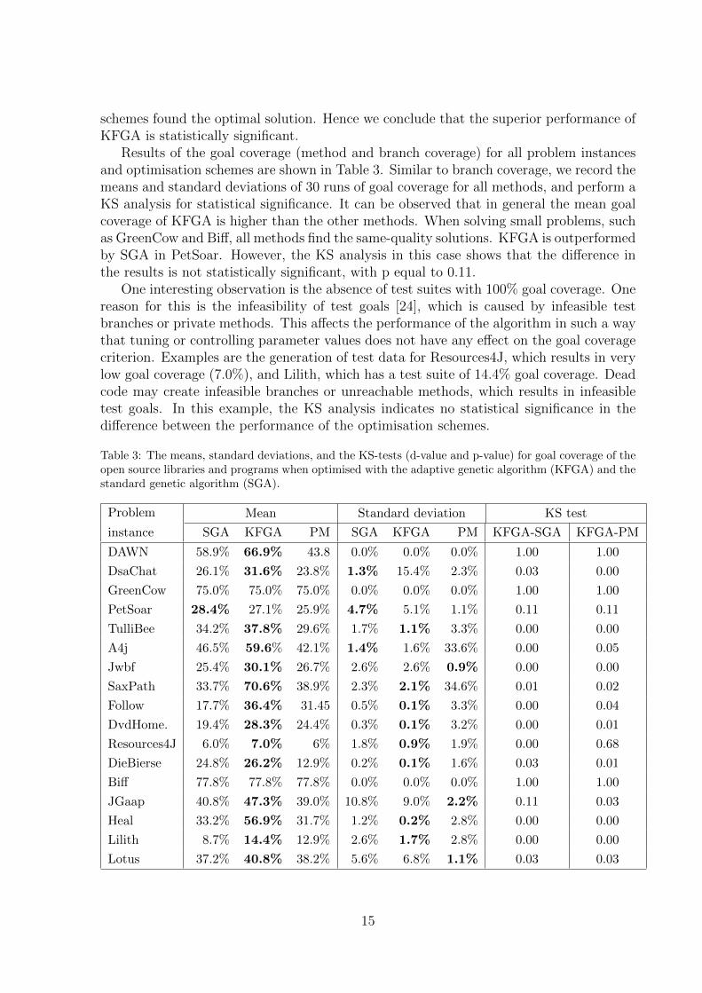
Results of the goal coverage (method and branch coverage) for all problem instancesand optimisation schemes are shown in Table 3. Similar to branch coverage, we record themeans and standard deviations of 30 runs of goal coverage for all methods, and perform aKS analysis for statistical significance. It can be observed that in general the mean goalcoverage of KFGA is higher than the other methods. When solving small problems, suchas GreenCow and Biff, all methods find the same-quality solutions. KFGA is outperformedby SGA in PetSoar. However, the KS analysis in this case shows that the difference inthe results is not statistically significant, with p equal to 0.11.

One interesting observation is the absence of test suites with 100% goal coverage. Onereason for this is the infeasibility of test goals [24], which is caused by infeasible testbranches or private methods. This affects the performance of the algorithm in such a waythat tuning or controlling parameter values does not have any effect on the goal coveragecriterion. Examples are the generation of test data for Resources4J, which results in verylow goal coverage (7.0%), and Lilith, which has a test suite of 14.4% goal coverage. Deadcode may create infeasible branches or unreachable methods, which results in infeasibletest goals. In this example, the KS analysis indicates no statistical significance in thedifference between the performance of the optimisation schemes.

Table 3: The means, standard deviations, and the KS-tests (d-value and p-value) for goal coverage of theopen source libraries and programs when optimised with the adaptive genetic algorithm (KFGA) and thestandard genetic algorithm (SGA).

Problem Mean Standard deviation KS test

instance SGA KFGA PM SGA KFGA PM KFGA-SGA KFGA-PM

DAWN 58.9% 66.9% 43.8 0.0% 0.0% 0.0% 1.00 1.00

DsaChat 26.1% 31.6% 23.8% 1.3% 15.4% 2.3% 0.03 0.00

GreenCow 75.0% 75.0% 75.0% 0.0% 0.0% 0.0% 1.00 1.00

PetSoar 28.4% 27.1% 25.9% 4.7% 5.1% 1.1% 0.11 0.11

TulliBee 34.2% 37.8% 29.6% 1.7% 1.1% 3.3% 0.00 0.00

A4j 46.5% 59.6% 42.1% 1.4% 1.6% 33.6% 0.00 0.05

Jwbf 25.4% 30.1% 26.7% 2.6% 2.6% 0.9% 0.00 0.00

SaxPath 33.7% 70.6% 38.9% 2.3% 2.1% 34.6% 0.01 0.02

Follow 17.7% 36.4% 31.45 0.5% 0.1% 3.3% 0.00 0.04

DvdHome. 19.4% 28.3% 24.4% 0.3% 0.1% 3.2% 0.00 0.01

Resources4J 6.0% 7.0% 6% 1.8% 0.9% 1.9% 0.00 0.68

DieBierse 24.8% 26.2% 12.9% 0.2% 0.1% 1.6% 0.03 0.01

Biff 77.8% 77.8% 77.8% 0.0% 0.0% 0.0% 1.00 1.00

JGaap 40.8% 47.3% 39.0% 10.8% 9.0% 2.2% 0.11 0.03

Heal 33.2% 56.9% 31.7% 1.2% 0.2% 2.8% 0.00 0.00

Lilith 8.7% 14.4% 12.9% 2.6% 1.7% 2.8% 0.00 0.00

Lotus 37.2% 40.8% 38.2% 5.6% 6.8% 1.1% 0.03 0.03

15

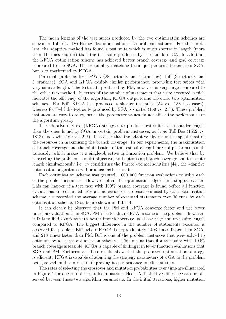
The mean lengths of the test suites produced by the two optimisation schemes areshown in Table 4. DvdHomevideo is a medium size problem instance. For this prob-lem, the adaptive method has found a test suite which is much shorter in length (morethan 11 times shorter) than the test suite produced by the standard GA. In addition,the KFGA optimisation scheme has achieved better branch coverage and goal coveragecompared to the SGA. The probability matching technique performs better than SGA,but is outperformed by KFGA.

For small problems like DAWN (28 methods and 4 branches), Biff (3 methods and2 branches), SGA and KFGA exhibit similar performance, producing test suites withvery similar length. The test suite produced by PM, however, is very large compared tothe other two method. In terms of the number of statements that were executed, whichindicates the efficiency of the algorithm, KFGA outperforms the other two optimisationschemes. For Biff, KFGA has produced a shorter test suite (54 vs. 183 test cases),whereas for Jwbf the test suite produced by SGA is shorter (160 vs. 217). These probleminstances are easy to solve, hence the parameter values do not affect the performance ofthe algorithm greatly.

The adaptive method (KFGA) struggles to produce test suites with smaller lengththan the ones found by SGA in certain problem instances, such as TulliBee (1652 vs.1813) and Jwbf (160 vs. 217). It is clear that the adaptive algorithm has spent most ofthe resources in maximising the branch coverage. In our experiments, the maximisationof branch coverage and the minimisation of the test suite length are not performed simul-taneously, which makes it a single-objective optimisation problem. We believe that byconverting the problem to multi-objective, and optimising branch coverage and test suitelength simultaneously, i.e. by considering the Pareto optimal solutions [44], the adaptiveoptimisation algorithms will produce better results.

Each optimisation scheme was granted 1, 000, 000 function evaluations to solve eachof the problem instances. However, often the optimisation algorithms stopped earlier.This can happen if a test case with 100% branch coverage is found before all functionevaluations are consumed. For an indication of the resources used by each optimisationscheme, we recorded the average number of executed statements over 30 runs by eachoptimisation scheme. Results are shown in Table 4.

It can clearly be observed that the PM and KFGA converge faster and use fewerfunction evaluation than SGA. PM is faster than KFGA in some of the problems, however,it fails to find solutions with better branch coverage, goal coverage and test suite lengthcompared to KFGA. The biggest difference in the number of statements executed isobserved for problem Biff, where KFGA is approximately 1493 times faster than SGA,and 213 times faster than PM. Biff is one of the problem instances that were solved tooptimum by all three optimisation schemes. This means that if a test suite with 100%branch coverage is feasible, KFGA is capable of finding it in fewer function evaluations thatSGA and PM. Furthermore, these results show that the proposed optimisation strategyis efficient. KFGA is capable of adapting the strategy parameters of a GA to the problembeing solved, and as a results improving its performance in efficient time.

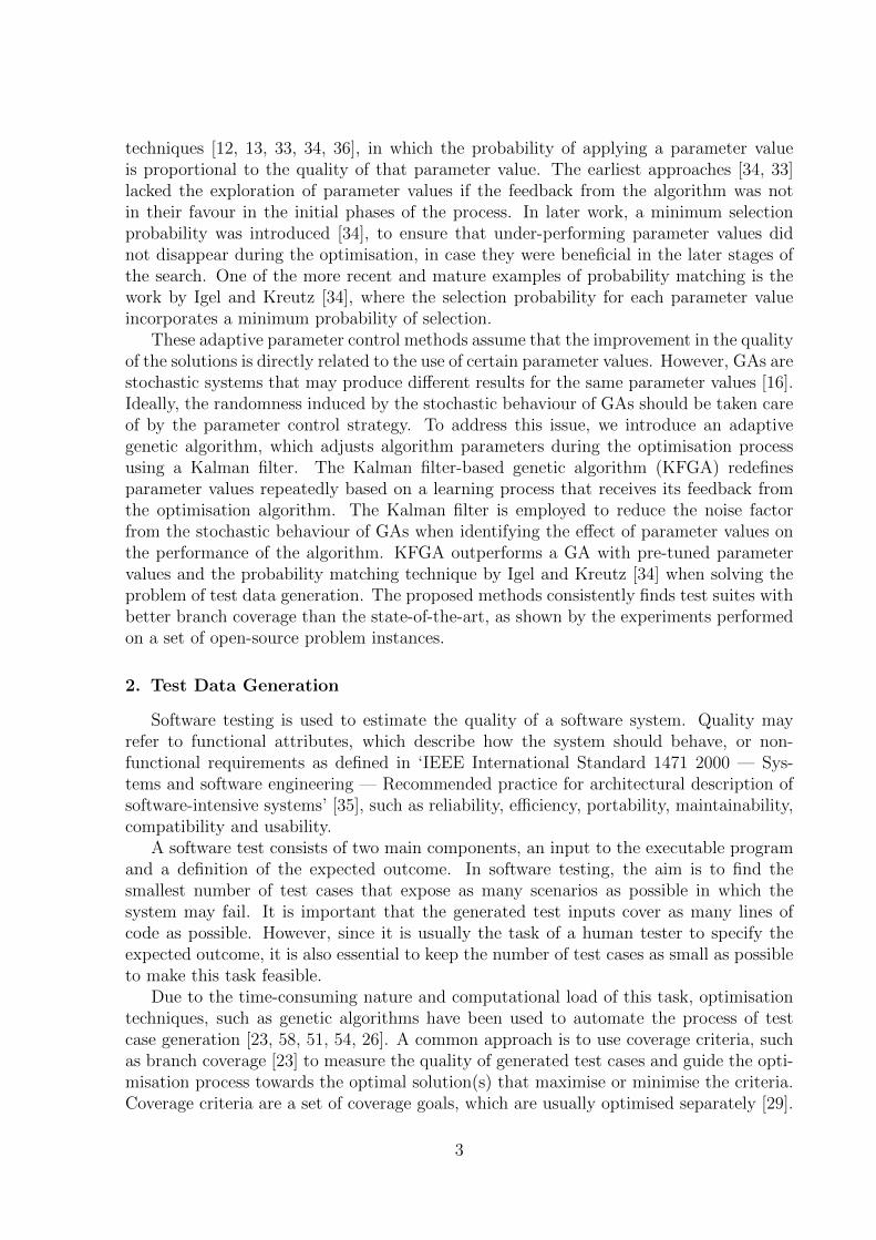
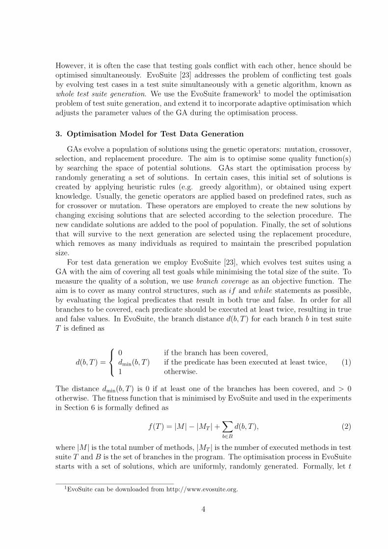
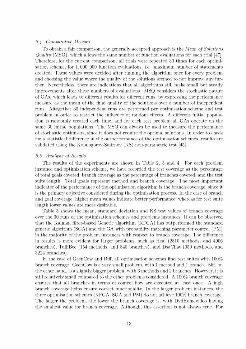
The rates of selecting the crossover and mutation probabilities over time are illustratedin Figure 1 for one run of the problem instance Heal. A distinctive difference can be ob-served between these two algorithm parameters. In the initial iterations, higher mutation

16

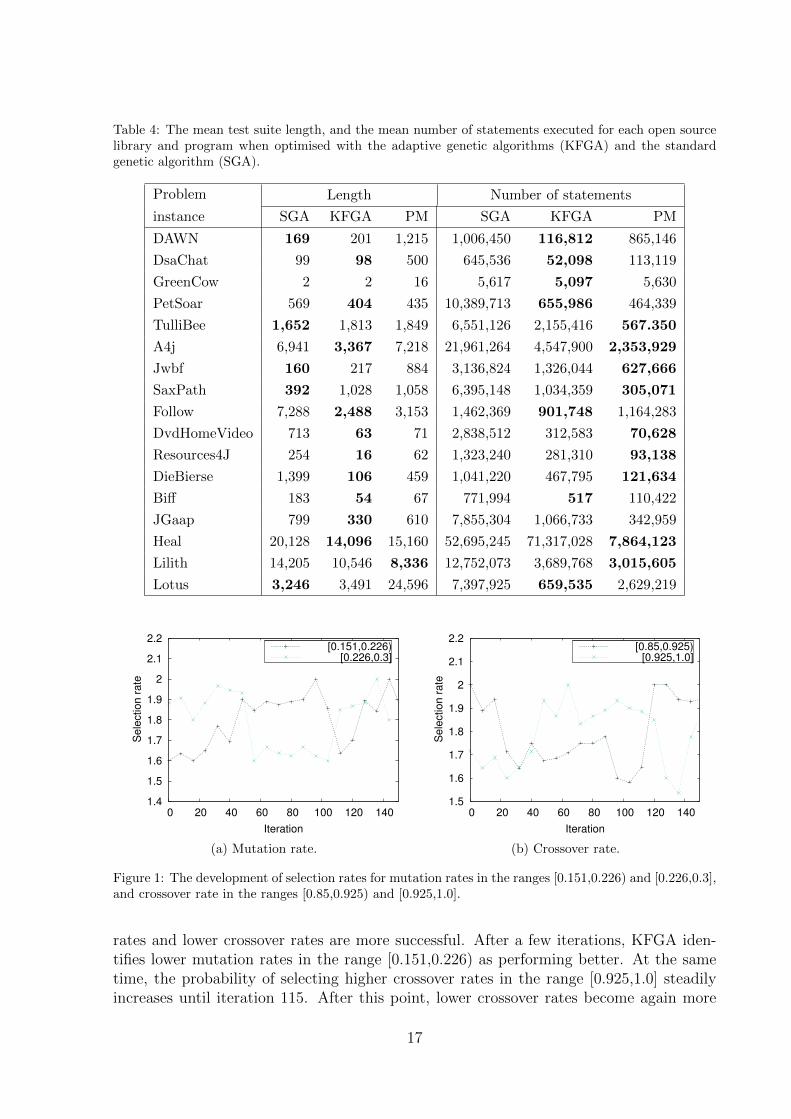
Table 4: The mean test suite length, and the mean number of statements executed for each open sourcelibrary and program when optimised with the adaptive genetic algorithms (KFGA) and the standardgenetic algorithm (SGA).

Problem Length Number of statements

instance SGA KFGA PM SGA KFGA PM

DAWN 169 201 1,215 1,006,450 116,812 865,146

DsaChat 99 98 500 645,536 52,098 113,119

GreenCow 2 2 16 5,617 5,097 5,630

PetSoar 569 404 435 10,389,713 655,986 464,339

TulliBee 1,652 1,813 1,849 6,551,126 2,155,416 567.350

A4j 6,941 3,367 7,218 21,961,264 4,547,900 2,353,929

Jwbf 160 217 884 3,136,824 1,326,044 627,666

SaxPath 392 1,028 1,058 6,395,148 1,034,359 305,071

Follow 7,288 2,488 3,153 1,462,369 901,748 1,164,283

DvdHomeVideo 713 63 71 2,838,512 312,583 70,628

Resources4J 254 16 62 1,323,240 281,310 93,138

DieBierse 1,399 106 459 1,041,220 467,795 121,634

Biff 183 54 67 771,994 517 110,422

JGaap 799 330 610 7,855,304 1,066,733 342,959

Heal 20,128 14,096 15,160 52,695,245 71,317,028 7,864,123

Lilith 14,205 10,546 8,336 12,752,073 3,689,768 3,015,605

Lotus 3,246 3,491 24,596 7,397,925 659,535 2,629,219

1.4

1.5

1.6

1.7

1.8

1.9

2

2.1

2.2

0 20 40 60 80 100 120 140

Se

lectio

n r

ate

Iteration

[0.151,0.226)[0.226,0.3]

(a) Mutation rate.

1.5

1.6

1.7

1.8

1.9

2

2.1

2.2

0 20 40 60 80 100 120 140

Se

lectio

n r

ate

Iteration

[0.85,0.925)[0.925,1.0]

(b) Crossover rate.

Figure 1: The development of selection rates for mutation rates in the ranges [0.151,0.226) and [0.226,0.3],and crossover rate in the ranges [0.85,0.925) and [0.925,1.0].

rates and lower crossover rates are more successful. After a few iterations, KFGA iden-tifies lower mutation rates in the range [0.151,0.226) as performing better. At the sametime, the probability of selecting higher crossover rates in the range [0.925,1.0] steadilyincreases until iteration 115. After this point, lower crossover rates become again more

17

successful than lower crossover rates. The selection probabilities of different ranges of mu-tation rate, on the other hand, become almost equal towards the end of the optimisationprocess. This means that the mutation operator is not discovering solutions with betterquality, despite the changes in the mutation rate. In the future, we will investigate therelationship between the behaviour of different parameter values and the structure of thesearch space of different problems instances.

7. Conclusion

We presented a Kalman filter-based genetic algorithm (KFGA) for solving the problemof test case generation in software testing. The method uses a Kalman filter to reducethe effect of the stochastic behaviour of GAs when estimating the appropriate parametervalues to use in each iteration of the optimisation process. KFGA was implementedin EvoSuite, a framework for whole test suite generation. A set of experiments wereconducted using open-source libraries and programs with different characteristics, such asnumber of methods, number of branches and number of testing goals. The performance ofthe KFGA was compared to the performance of a standard GA with pre-tuned parametersetting and a GA with probability matching parameter control. Results showed that theadaptive method outperformed the standard GA and the probability matching methodover the majority of the problem instances.

In some cases, the difference in the performance of the algorithms was not statisticallysignificant. This usually happens either when problems are easy to solve by all optimisa-tion schemes, so controlling parameter values does not have any benefit, or when branchesare infeasible, such that no method is able to find any solutions. In general, KFGA notonly performed better than the other method, but also used fewer function evaluations,which reflects its efficiency in adapting the search strategy to the problem being solved. Inthe future, the test suite generation problem will be converted to a multi-objective prob-lem, where branch coverage and the length of the test suite will be modelled as conflictingobjectives and optimised simultaneously.

Acknowledgements

We would like to thank Gordon Fraser and the rest of the team who developed EvoSuitefor making the source code available. We wish to acknowledge Monash University for theuse of their Nimrod software in this work. The Nimrod project has been funded by theAustralian Research Council and a number of Australian Government agencies, and wasinitially developed by the Distributed Systems Technology. This research was supportedunder Australian Research Council’s Discovery Projects funding scheme (project numberDE140100017). We would like to thank several anonymous reviewers who helped improvethe quality of this work.

References

[1] Wasif Afzal, Richard Torkar, and Robert Feldt. A systematic review of search-basedtesting for non-functional system properties. Information & Software Technology,51(6):957–976, 2009.

18

[2] Moataz A. Ahmed and Irman Hermadi. GA-based multiple paths test data generator.Computers & OR, 35(10):3107–3124, 2008.

[3] Aldeida Aleti. An adaptive approach to controlling parameters of evolutionary algo-rithms. PhD thesis, Swinburne University of Technology, 2012.

[4] Aldeida Aleti, Barbora Buhnova, Lars Grunske, Anne Koziolek, and Indika Mee-deniya. Software architecture optimization methods: A systematic literature review.IEEE Transactions on Software Engineering, 39(5):658–683, 2013.

[5] Aldeida Aleti, Lars Grunske, Indika Meedeniya, and Irene Moser. Let the ants deployyour software - an ACO based deployment optimisation strategy. In ASE, pages 505–509. IEEE Computer Society, 2009.

[6] Aldeida Aleti and Irene Moser. Entropy-based adaptive range parameter control forevolutionary algorithms. In Proceeding of the fifteenth annual conference on Geneticand evolutionary computation conference, GECCO ’13, pages 1501–1508. ACM, 2013.

[7] Andrea Arcuri and Gordon Fraser. Parameter tuning or default values? An empiricalinvestigation in search-based software engineering. Empirical Software Engineering,18(3):594–623, 2013.

[8] Thomas Back. The interaction of mutation rate, selection, and self-adaptation withina genetic algorithm. In Parallel Problem Solving from Nature 2,PPSN-II, pages 87–96. Elsevier, 1992.

[9] Thomas Back, Agoston Endre Eiben, and Nikolai A. L. van der Vaart. An empiricalstudy on GAs without parameters. In Parallel Problem Solving from Nature – PPSNVI (6th PPSN’2000), volume 1917 of Lecture Notes in Computer Science (LNCS),pages 315–324. Springer-Verlag (New York), 2000.

[10] Thomas Back and Martin Schutz. Intelligent mutation rate control in canonicalgenetic algorithms. Lecture Notes in Computer Science, 1079:158–167, 1996.

[11] Jorge Cervantes and Christopher R. Stephens. Limitations of existing mutation rateheuristics and how a rank GA overcomes them. IEEE Transcation on EvolutionaryComputation, 13(2):369–397, 2009.

[12] David Corne, Martin J. Oates, and Douglas B. Kell. On fitness distributions andexpected fitness gain of mutation rates in parallel evolutionary algorithms. In ParallelProblem Solving from Nature – PPSN VII (7th PPSN’02), volume 2439 of LectureNotes in Computer Science (LNCS), pages 132–141. Springer-Verlag, 2002.

[13] Lawrence Davis. Adapting operator probabilities in genetic algorithms. In Pro-ceedings of the Third International Conference on Genetic Algorithms, pages 70–79.Morgan Kaufman, 1989.

[14] Kenneth A. De Jong. An analysis of the behavior of a class of genetic adaptivesystems. PhD thesis, University of Michigan, 1995.

19

[15] Kalyanmoy Deb and Hans-Georg Beyer. Self-adaptive genetic algorithms with sim-ulated binary crossover. Evolutionary Computation, 9(2):197–221, 2001.

[16] Kenneth DeJong. Parameter setting in EAs: a 30 year perspective. In Fernando G.Lobo, Claudio F. Lima, and Zbigniew Michalewicz, editors, Parameter Setting inEvolutionary Algorithms, volume 54 of Studies in Computational Intelligence, pages1–18. Springer, 2007.

[17] Agoston Endre Eiben, Robert Hinterding, and Zbigniew Michalewicz. Parametercontrol in evolutionary algorithms. IEEE Transations on Evolutionary Computation,3(2):124–141, 2007.

[18] Agoston Endre Eiben and Martijn C. Schut. New ways to calibrate evolutionary algo-rithms. In Patrick Siarry and Zbigniew Michalewicz, editors, Advances in Metaheuris-tics for Hard Optimization, Natural Computing Series, pages 153–177. Springer, 2008.

[19] Agoston Endre Eiben and Selmar K. Smit. Parameter tuning for configuring andanalyzing evolutionary algorithms. Swarm and Evolutionary Computation, 1(1):19–31, 2011.

[20] Raziyeh Farmani and Jonathan A. Wright. Self-adaptive fitness formulation for con-strained optimization. IEEE Transaction Evolutionary Computation, 7(5):445–455,2003.

[21] Javier Ferrer, J. Francisco Chicano, and Enrique Alba. Evolutionary algorithms forthe multi-objective test data generation problem. Softw, Pract. Exper, 42(11):1331–1362, 2012.

[22] Alvaro Fialho, Luis Da Costa, Marc Schoenauer, and Michele Sebag. Analyzingbandit-based adaptive operator selection mechanisms. Annals of Mathematics andArtificial Intelligence - Special Issue on Learning and Intelligent Optimization, 2010.

[23] Gordon Fraser and Andrea Arcuri. Whole test suite generation. IEEE Transactionson Software Engineering, 39(2):276–291, 2013.

[24] A. Goldberg, T.C. Wang, and D. Zimmerman. Applications of feasible path analysisto program testing. In ACM SIGSOFT International Symposium in Software Testingand Analysis, Proceedings, pages 80–94, 1994.

[25] David E. Goldberg. Genetic Algorithms in Search, Optimization and Machine Learn-ing. Addison-Wesley, 1989.

[26] Dunwei Gong and Yan Zhang. Generating test data for both path coverage and faultdetection using genetic algorithms. Frontiers of Computer Science, 7(6):822–837,2013.

[27] John J. Grefenstette. Optimization of control parameters for genetic algorithms.IEEE Transactions on Systems, Man, and Cybernetics, SMC-16(1):122–128, 1986.

20

[28] Lars Grunske. Identifying ”good” architectural design alternatives with multi-objective optimization strategies. In International Conference on Software Engi-neering, ICSE, pages 849–852. ACM, 2006.

[29] Mark Harman, Sung Gon Kim, Kiran Lakhotia, Phil McMinn, and Shin Yoo. Opti-mizing for the number of tests generated in search based test data generation withan application to the oracle cost problem. In ICST Workshops, pages 182–191. IEEEComputer Society, 2010.

[30] Mark Harman, Kiran Lakhotia, and Phil McMinn. A Multi-Objective Approach ToSearch-Based Test Data Generation. In Dirk Thierens, editor, 2007 Genetic andEvolutionary Computation Conference (GECCO’2007), volume 1, pages 1098–1105,London, UK, July 2007. ACM Press.

[31] Mark Harman and Phil McMinn. A theoretical and empirical study of search-basedtesting: Local, global, and hybrid search. IEEE Transaction Software Engineering,36(2):226–247, 2010.

[32] J. Hesser and R. Manner. Towards an optimal mutation probability for geneticalgorithms. Lecture Notes in Computer Science, 496:23–32, 1991.

[33] Tzung-Pei Hong, Hong-Shung Wang, and Wei-Chou Chen. Simultaneously applyingmultiple mutation operators in genetic algorithms. Journal of Heuristics, 6(4):439–455, 2000.

[34] Christian Igel and Martin Kreutz. Operator adaptation in evolutionary computationand its application to structure optimization of neural networks. Neurocomputing,55(1-2):347–361, 2003.

[35] ISO/IEC. IEEE international standard 1471 2000 - systems and software engineering- recommended practice for architectural description of software-intensive systems,2000.

[36] Bryant A. Julstrom. What have you done for me lately? Adapting operator proba-bilities in a steady-state genetic algorithm. In Proceedings of the Sixth InternationalConference on Genetic Algorithms, pages 81–87, San Francisco, CA, 1995. MorganKaufmann.

[37] R. E. Kalman. A new approach to linear filtering and predictive problems. Transac-tions ASME, Journal of basic engineering, (82):34–45, 1960.

[38] F. G. Lobo and David E. Goldberg. Decision making in a hybrid genetic algorithm.In Proceedings of the Congress on Evolutionary Computation, pages 121–125. IEEEPress, 1997.

[39] Fernando G. Lobo. Idealized dynamic population sizing for uniformly scaled prob-lems. In 13th Annual Genetic and Evolutionary Computation Conference, GECCO2011, Proceedings, pages 917–924. ACM, 2011.

21

[40] Stefan Mairhofer, Robert Feldt, and Richard Torkar. Search-based software testingand test data generation for a dynamic programming language. In Natalio Krasnogorand Pier Luca Lanzi, editors, 13th Annual Genetic and Evolutionary ComputationConference, GECCO 2011, Proceedings, Dublin, Ireland, July 12-16, 2011, pages1859–1866. ACM, 2011.

[41] Phil McMinn. Search-based software test data generation: a survey. Softw. Test,Verif. Reliab, 14(2):105–156, 2004.

[42] Melanie Mitchell. An Introduction to Genetic Algorithms. Complex Adaptive Sys-tems. MIT-Press, Cambridge, 1996.

[43] Christopher K. Monson and Kevin D. Seppi. The kalman swarm: A new approach toparticle motion in swarm optimization. In Genetic and Evolutionary Computation,volume 3102 of Lecture Notes in Computer Science, pages 140–150. Springer-Verlag,2004.

[44] Vilfredo Pareto. CoursD’Economie Politique. F. Rouge, 1896.

[45] A. N. Pettitt and M. A. Stephens. The kolmogorov-smirnov goodness-of-fit statisticwith discrete and grouped data. Technometrics, 19(2):205–210, 1977.

[46] Outi Raiha. A survey on search-based software design. Computer Science Review,4(4):203–249, 2010.

[47] Ronald L. Rardin and Reha Uzsoy. Experimental evaluation of heuristic optimizationalgorithms:A tutorial. Journal of Heuristics, 7(3):261–304, 2001.

[48] J. David Schaffer, Richard A. Caruana, Larry J. Eshelman, and Rajarshi Das. Astudy of control parameters affecting online performance of genetic algorithms forfunction optimization. In Proceedings of the Third International Conference on Ge-netic Algorithms, pages 51–60. Morgan Kaufman, 1989.

[49] D. Schlierkamp-Voosen and H. Muhlenbein. Strategy adaptation by competing sub-populations. Lecture Notes in Computer Science, 866:199–208, 1994.

[50] Jim Smith and Terence C. Fogarty. Self adaptation of mutation rates in a steadystate genetic algorithm. In International Conference on Evolutionary Computation,pages 318–323, 1996.

[51] Praveen Ranjan Srivastava. Optimisation of software testing using genetic algorithm.IJAISC, 1(2/3/4):363–375, 2009.

[52] Christopher R. Stephens, I. Garcia Olmedo, J. Mora Vargas, and Henri Waelbroeck.Self-adaptation in evolving systems. Artificial Life, 4(2):183–201, 1998.

[53] Phillip D. Stroud. Kalman-extended genetic algorithm for search in nonstationaryenvironments with noisy fitness evaluations. IEEE Transactions on EvolutionaryComputation, 5(1):66–77, 2001.

22

[54] Yeresime Suresh and Santanu Ku. Rath. A genetic algorithm based approach for testdata generation in basis path testing. CoRR, abs/1401.5165, 2014.

[55] Dirk Thierens. Adaptive mutation rate control schemes in genetic algorithms. InProceedings of the 2002 Congress on Evolutionary Computation CEC2002, pages980–985. IEEE Press, 2002.

[56] Andrew Tuson and Peter Ross. Adapting operator settings in genetic algorithms.Evolutionary Computation, 6(2):161–184, 1998.

[57] Darrell Whitley. The GENITOR algorithm and selection pressure: Why rank-basedallocation. In James D. Schaffer, editor, Proc. of the Third Int. Conf. on GeneticAlgorithms, pages 116–121, San Mateo, CA, 1989. Morgan Kaufmann.

[58] Andreas Windisch. Search-based test data generation from stateflow statecharts.In Genetic and Evolutionary Computation Conference, GECCO 2010, Proceedings,pages 1349–1356. ACM, 2010.

23