World War II and African AmericanSocioeconomic Progress

Andreas Ferrara∗

January 11, 2019

Abstract

This paper argues that the unprecedented socioeconomic rise of African Ameri-cans at mid-century was causally related to the labor shortages induced by WWII.Combining novel military and Census data in a difference-in-differences setting, re-sults show that counties with an average casualty rate among semi-skilled whitesexperienced a 13 to 16% increase in the share of blacks in semi-skilled jobs. Thecasualty rate also had a positive reduced form effect on wages, home ownership,house values, and education for blacks. Using Southern survey data, IV regressionresults indicate that individuals in affected counties had more interracial friendshipsand reduced preferences for segregation in 1961. This is an example for how betterlabor market opportunities can improve both economic and social outcomes of adisadvantaged minority group.

JEL codes: J15, J24, N42Keywords: African-Americans; Inequality; Race-Relations; World War II.

∗University of Warwick, Department of Economics and CAGE. Email: a.ferrara@warwick.ac.ukI thank Cihan Artunc, Martha Bailey, Sascha O. Becker, Leah Boustan, Clement de Chaisemartin, JamesFenske, Price Fishback, Carola Frydman, Stephan Heblich, Taylor Jaworski, Christoph Konig, FelixKonig, Luigi Pascali, Steve Pischke, Patrick Testa, Nico Voigtlander, Fabian Waldinger, and seminarparticipants at the University of Arizona, London School of Economics, Pompeu Fabra, Warwick, andat the 3rd ASREC Europe conference, 56th Cliometric Society Conference, 29th EALE conference, EEA-ESEM Congress 2018, 78th EHA annual meeting, EHS conference 2018, IZA World Labor Conference2018, RES conference 2018, 18th World Economic History Congress, 23rd Spring Meeting of YoungEconomists, 7th IRES Graduate Student Workshop, 3rd RES Symposium of Junior Researchers, and the20th IZA Summer School for valuable comments and discussions.

1

1 Introduction

The gap in the social and economic outcomes and opportunities between blacks and

whites has been a constant in the United States.1 Differences in wages (Bayer and

Charles, 2018) and residential segregation (Boustan, 2010) follow stubbornly persistent

historic patterns. Changes over the last century have been episodic. The situation for

blacks before 1940 was stagnant (Myrdal, 1944), while Margo (1995) and Maloney (1994)

documented sharp improvements from the 1940s to 60s which continued through the Civil

Rights era (Donohue and Heckman, 1991; Wright, 2013), followed by the decline in black

economic fortunes after the mid-1970s (see Bound and Freeman, 1992).

These episodes are reflected in the skill composition of black men and are shown in

figure 1. The 1940s and the immediate post-war decades stand out. Between 1940 and

1950, the share of semi-skilled employment among blacks almost doubled. In this one

decade alone, blacks made more occupational progress than in the 70 years since the end

of the Civil War. Collins (2001) called this period a turning point in African American

economic history.

In this paper I study the origins of this turning point, and the effect of the unprece-

dented occupational upgrade on the economic and social status of blacks in the U.S. My

main hypothesis is that higher WWII casualty rates among semi-skilled white workers

drove the occupational upgrade of black workers. These deaths and the tight labor mar-

ket during the war years opened up employment opportunities from which blacks had

been barred in the past. I argue that the casualty-induced occupational upgrade not only

improved several economic outcomes, such as wages, house values, or education, but that

it also had a positive effect on blacks’ social status.

African American economic progress during the 1940-60s has been studied with re-

spect to the narrowing of the black-white wage gap (Margo, 1995; Maloney, 1994; Bailey

and Collins, 2006), migration and urbanization (Boustan, 2009, 2010, 2016), home owner-

ship (Collins and Margo, 2011; Boustan and Margo, 2013; Logan and Parman, 2017), and

education (Smith, 1984; Turner and Bound, 2003). Our knowledge about the root causes

of this sudden success is less developed and especially its relation to the occupational

upgrade is less well studied (Margo, 1995).

1For an overview of recent trends, especially with respect to the social outcomes and interactionsbetween blacks and whites, see Fryer (2007).

2

The occupational upgrade at mid-century coincides with several major events, in-

cluding the Great Migration, the first anti-discrimination policies enforced by the Fair

Employment Practice Committee (FEPC), and World War II. This makes it challenging

to isolate any single cause. The Great Migration to the North and West, which began dur-

ing the 1940s, substantially benefited African Americans who migrated (Boustan, 2009,

2016). Panel (b) of figure 1 suggests tough that the occupational gains were not solely

concentrated in the North. The FEPC was disbanded shortly after the war and did not

have a strong impact in the South (Collins, 2001).

Previous work on the labor market and educational effects of the war has primarily

focused on women (Goldin, 1991; Acemoglu et al., 2004; Goldin and Olivetti, 2013;

Jaworski, 2014; Shatnawi and Fishback, 2018). Two exceptions are Collins (2000) who

studies the role of veteran status in black males’ economic mobility during the 1940s,

and Turner and Bound (2003) who estimate the educational effects of the G.I. Bill on

black veterans. The occupational upgrading, however, was mostly driven by non-veterans

and especially by the one million blacks who entered semi-skilled employment during the

war years (Wolfbein, 1947). The war therefore provides a potential explanation for this

development which goes beyond the gains made by veterans.

This paper makes three contributions to the literature. First, I construct a novel data

set of military casualty records and combine them with Southern county-level Census

data from 1920 to 1970. Difference-in-differences results provide causal evidence that

the occupational upgrade of blacks was driven by higher WWII casualty rates among

semi-skilled white workers. Using casualty instead of draft rates is motivated by the fact

that they are free from the displacement effects created by soldiers returning after the

war.2 The effect of the draft on female labor supply was temporary as returning soldiers

displaced most female workers again (see Acemoglu et al., 2004). Casualties instead have

the potential to explain the persistent employment effects seen in figure 1.

Results show that counties with an average WWII casualty rate among semi-skilled

whites increased the share of blacks in semi-skilled jobs by 13 to 16% relative to the pre-

war mean. The average casualty rate can explain between 75 to 90% of the overall inflow

of blacks into this occupational group between 1940 and 1950. The effect is persistent

and lasts until the end of the sample period in 1970. The results are robust to several

2Given the previous literature of WWII and the draft, I always control for the draft rate as well.

3

specifications, and placebo tests provide evidence that they are not driven by casualties

among race or skill-groups.

To generalize these results to the entire country, I repeat the previous analysis using

individual level Census data from 1920 to 1970 in a triple differences estimation framework

with the casualty rate treatment being assigned at the commuting zone level. This is to

show that occupational upgrading did occur for blacks (both in the South and outside) but

not for whites. This is evidence that the war casualties not merely induced a labor supply

shock, but that it removed barriers to entry into these occupations which blacks had faced

before the war. The individual level data also have the advantage that they can be used

to more meticulously probe for effect heterogeneity. In particular, I provide evidence that

the upgrading was not driven by differential cross-state migration or education patterns

for blacks, and that the upgrading effect was especially concentrated in manufacturing.

There was no effect in placebo sectors that remained segregated throughout and after the

war such as retail or telecommunications.

Second, I use the same triple differences estimation framework to show that the out-

comes considered by previous studies analyzing black economic progress at mid-century

are systematically related with the WWII casualty rate among semi-skilled whites. The

outcomes include wages, urbanization, migration, home ownership, house values, and ed-

ucational attainment for blacks.3 The relationship between the casualty rates, as driver of

the black occupational upgrade, and the economic outcomes is strongest for house values,

wages, and education. Effects on home ownership are only short-lived and urbanization

does not appear to be affected at all. Blacks living in areas with higher casualty rates

had a lower probability for migrating out of their birth state. This is likely because the

improvements in local employment opportunities reduced the need to relocate to other

states. The results are robust to several specifications and inclusion of different types

of time trends, and are not driven by differential changes in mobility or educational at-

tainment across blacks and whites, or mere North-South differences. The majority of the

outcomes that have been considered in studies of black economic progress at mid-century

can therefore be directly linked to the war as one of their common root causes.

Third, I return to the Southern-specific context and estimate the effect of the occupa-

3For work on wages see Maloney (1994), Margo (1995), and Bailey and Collins (2006), for migrationBoustan (2016), for home ownership Collins and Margo (2011), Boustan and Margo (2013), and Loganand Parman (2017), for education Smith (1984), and Turner and Bound (2003).

4

tional upgrade on blacks’ social standing. For the analysis I use individual-level survey

data on 1,068 black and white individuals from 24 Southern counties in 1961. Despite

the relatively small sample size, the timing is ideal for studying this question as the data

were collected before the major Civil Rights legislation, mainly the Civil Rights Act of

1964, as well as before the outbreak of violence during the Civil Rights protests. I instru-

ment the occupational upgrade with the WWII casualty rates in instrumental variables

regressions in order to provide causal estimates. Both black and white respondents who

live in areas with a casualty-induced occupational upgrade of African Americans are sig-

nificantly more likely to have an interracial friendship, to live in mixed-race areas, and

to favor integration over segregation. Previous work on the Civil Rights movement has

argued that it was the Civil Rights Act of 1964 which has brought about the major break

from past trends in the economic and social segregation of blacks (Wright, 2013). I offer

a new viewpoint wherein these breaks already occur during and due to WWII.

OLS and IV results are similar and estimate an increase in respondents’ probability

of reporting an interracial friendship, of living in a mixed-race area, and a of favoring

integration over segregation. The results are sizable relative to the outcome averages.

They are not driven solely by black respondents but are similar across the two groups,

and they hold up also for small violations of the exclusion restriction using the test by

Conley et al. (2012).

Studying the relationship between the war and black socioeconomic progress shows

how improvements in labor market opportunities for a disadvantaged minority group can

positively affect both economic and social outcomes for members of this group. This is

a relevant topic for countries with economically and socially segregated minority groups

given a literature which shows that such fragmentation is detrimental for societal out-

comes (see Alesina et al., 1999). It is also related to the debate about the effectiveness

of affirmative action policies (Coate and Loury, 1993). Importantly, the casualty-induced

shock to blacks’ labor market opportunities here is not coming from the potentially en-

dogenous choices of a policy-maker but from a natural experiment. Hence this setting

can allow to more cleanly identify the economic and social spillover effects of policies that

seek to improve the labor market opportunities for a minority group.

The remainder of the paper is structured as follows. Section 2 provides a brief overview

of African American economic history in the 20th century to highlight previous directions

5

of research and to put this paper into context. Section 3 describes the enlistment and

casualty data, features of the draft system, how the data are linked, and how they are

used to construct WWII casualty rates by skill group and race. It then outlines the

difference-in-differences regression framework used to estimate the effect of casualties

among semi-skilled whites on the promotion of blacks into semi-skilled work. This is

followed by an extension of the analysis to the whole country using individual level Cen-

sus data in a triple differences setting. Section 4 uses the same individual level Census

data and estimation strategy for the South and the entire U.S. to relate the casualty rate

measure at the commuting zone level to previously studied economic outcomes regarding

African American economic progress. Section 5 describes the data and instrumental vari-

ables framework to estimate the effect of the occupational upgrade on black-white social

relations in a cross-sectional survey in the South in 1961. The final section concludes.

2 Black Economic Progress Pre- and Post-WWII

Myrdal (1944) provides an account of the pre-war conditions of blacks in the U.S.:

“They own little property; even their household goods are mostly inadequate and dilapi-

dated. Their incomes are not only low but irregular. They thus live from day to day and

have a scant security for the future.” (p. 205). This is reflected in figure 1. Before 1940,

70-90% of black men were employed in low-skilled occupations. In the Southern states,

the share of black men in semi-skilled occupations rose by 8 p.p. between 1870 and 1940

but increased by 11.4 p.p. from 1940 to 1950. Blacks made more economic progress in

the decade of WWII than in the last seven decades after the end of the Civil War. This

exceptional period has attracted the attention of labor economists and economic histori-

ans alike. Economic progress for blacks during the 1940s and 1950s has been documented

for wages and inequality, education, urbanization and home ownership, among others.

Margo (1995) and Maloney (1994) make two seminal contributions that assess the

factors behind black-white wage convergence between 1940-50 in a wage decomposition

exercise. Margo (1995) shows that the decrease in black-white wage differentials can be

attributed to the Great Compression,4 but also to the shift of African American workers

into better-paying jobs, migration to the North and better education opportunities for

4The Great Compression refers to the significant reduction of the dispersion of wages across andwithin education, experience, and occupation groups (see Goldin and Margo, 1992).

6

blacks. Also Maloney (1994) reaches this conclusion in a similar decomposition exercise.

Bailey and Collins (2006) provide a wage decomposition for African-American women in

the 1940s. They also document a rapid decrease in the racial wage gap in this period

and attribute it to occupational shifts for this group. However, none of these studies

examined the causal roots behind the occupational upgrading.

Education for blacks at mid-century developed more steadily. Results by Smith (1984)

do not show a particular uptick in educational attainment during the 1940-50 period. The

share of illiteracy among blacks declined from 16.3 to 11.5% between 1930-40, but reduced

only from 11.5 to 10.2 % between 1940-52 (Smith, 1984). The base for later economic

success was founded in improved access and quality of schooling in the earlier part of

the century. Aaronson and Mazumder (2011) show that the spread of Rosenwald schools

in the South improved educational attainment of blacks with access to such facilities by

one year in rural areas for those born between 1910 and 1925. They can explain 40% of

the black-white convergence in education for these cohorts. College education for blacks

started to increase slowly after WWII (Collins and Margo, 2006), but only increased at

a more rapid pace after the 1960s. Turner and Bound (2003) provide evidence that the

G.I. Bill significantly increased college education for both black and white men but not

for those black veterans who were born in the South.

Outmigration of blacks from the South to Northern cities and its effects on local

labor and housing markets has been well documented. Migration from the rural South to

the Northern industrial centers during WWII was an opportunity for economic elevation

through better employment opportunities (Boustan, 2016). However, while migrants

benefited, the additional competition impeded the wage growth of black workers who

already lived in the North (Boustan, 2009). The arrival of Southern blacks also produced

a response by whites. Boustan (2010) estimates that 2.7 whites departed for each black

arrival in a Northern city. White flight might have contributed to increased black home

ownership in the city centers, according to Boustan and Margo (2013). Generally, home

ownership has increased significantly for African Americans after WWII, though benefits

from the G.I. Bill do not appear to drive this result (Logan and Parman, 2017). Moving

North was not always related with positive outcomes. For some, this was correlated with

higher levels of child mortality or incarceration instead (Eriksson and Niemesh, 2016;

Eriksson, 2018).

7

While there are good explanations for the evolution of black education and the mi-

gration patterns at mid-century, there is still little insight into the unprecedented occu-

pational upgrade of African Americans. It cannot be explained by education because

black education expanded more gradually and long before the war. Migration alone is

not a sufficient explanation as occupational upgrading not only occurred in the North:

panel (b) of figure 1 documents a very similar pattern for the South. Institutional factors

played a role in helping blacks gain better employment or to reduce inequality, but these

factors do not appear to play a major role in the South. The Fair Employment Practice

Committee (FEPC) generated substantial employment and wage gains for blacks but was

ineffective in the South (Collins, 2001). The FEPC was disbanded shortly after the war

and nationwide affirmative action policies were only implemented with or after the Civil

Rights Act.

Another strand of the literature mainly attributes post-war black economic and so-

cial progress to the Civil Rights movement (see Wright, 2013). Several Supreme Court

decisions and laws, most notably the Civil Rights Act of 1964, sought to improve the

economic and social equality of African Americans. This includes enforcement of voting

rights and interracial marriage after the 1965 Voting Rights Act and the 1967 Supreme

Court ruling in Loving versus Virginia, respectively. The affirmative action policies of

the 1960s played an important role in desegregating firms (Miller, 2017). Wright (2013)

argues that the Civil Rights movement was the main breaking point from past trends and

that it set in motion the process of economic and social integration of blacks. Despite the

importance of the Civil Rights Act for the social and economic progress made by blacks,

figure 1 suggests that the break in occupational segregation had already occurred during

the 1940s.

If migration, improved education, and other regulatory and institutional factors do

not explain the sudden and large occupational shift from low- to semi-skilled jobs for

African Americans, the question then is what other factor could have been at the root

of this phenomenon. A natural starting point is World War II. Using data from the

Civil War, Larsen (2015) provides evidence for how war related labor shortages reduced

lynchings of blacks and increased political participation. The labor market effects of

World War II, and in particular of the draft, have been extensively studied for women

(Goldin, 1991; Acemoglu et al., 2004; Goldin and Olivetti, 2013; Jaworski, 2014; Shatnawi

8

and Fishback, 2018). The effect of the war on African Americans’ economic progress has

received comparatively little attention.

Labor economists at the time, such as Wolfbein (1947), observed that a, “significant

shift occurred from the farm to the factory as well as considerable upgrading of Negro

workers, many of whom received their first opportunity to perform basic factory oper-

ations in a semiskilled or skilled capacity” (p. 663). He attributed this to the labor

shortages during the war. Likewise, Weaver (1945) describes how labor shortages in the

aircraft industry opened job opportunities for blacks beyond low-skilled work. If the labor

shortages during the war were the only reason, why did the blacks maintain their labor

market gains in the post-war period unlike women? From the historic accounts it appears

that the war played a significant role in the skill-upgrade of blacks which translated into

other economic gains such as higher wages (Maloney, 1994; Margo, 1995; Collins, 2000),

but the precise channel of this lasting effect is not well known. This has been an under-

studied part of black economic history: “The story of black occupational upgrading is

somewhat less well known than the story of black migration” (Margo, 1995, p. 472).

3 White War Casualties and the Black Occupational Upgrade

3.1 Computing a Casualty Rate for Semi-Skilled Whites

To compute county-specific casualty rates among semi-skilled whites, I match two

data sources, the WWII Enlistment Records and the WWII Honor List of Dead and

Missing, for the Army and Army Air Force.5 The Army kept meticulous records of their

drafted and enlisted soldiers during the war. Upon entry, an IBM punch card would

store a soldier’s name, unique Army serial number, age, education, race, marital status,

residence, date and place of entry, and their pre-war occupation codified in three-digit

groups using the Dictionary of Occupational Titles of 1939. The National Archives and

Records Administration digitized these enlistment records.

The data do not contain soldiers in other service branches such as the Navy, Marines,

or Coast Guard. However, the 8.3 million individuals in the Army comprise the majority

of the 10 million drafted men during World War II. Due to the high manpower demands

by the armed forces there was almost no scope for drafted soldiers to choose a service

5The Air Force only became an independent service branch after the war in 1947.

9

branch (Flynn, 1993). Volunteering provided more choice regarding the branch of service

but was forbidden in 1942 to give the military more control over who entered into service

(Flynn, 1993). The removal of volunteering came before the largest battles and casualties

were sustained but after the majority of the drafting was completed (see figure 2). It

therefore would have been difficult to form a prior as to which service branch was the

least dangerous in order to enlist strategically.

Deferments were only obtained by fathers with dependents, workers in war-related

industries and farmers, or conscientious objectors. Out of 40 million men who had been

assessed by their local draft boards only 11,896 men registered as conscientious objec-

tors based on religious reasons (Flynn, 1993). Given that the draft was enacted during

peacetime, it had to be significantly more just and equal than the prior drafts to pass

the substantial resistance by politicians and the public. Going to college or buying out

was not possible. Kriner and Shen (2010) show that there was no significant difference

in casualty rates across socioeconomic groups during WWII. Only from the Korean War

onwards such a gap emerged.

Generally, the willingness to join the war effort was high. Out of 16 million WWII

soldiers some 50,000 deserted compared to the 200,000 out of 2.5 million Civil War soldiers

(Glass, 2013). There is little historic evidence that draft evasion and avoidance were a

major issue during WWII, especially after Pearl Harbor.6

To supplement the enlistment data with information about a soldier’s survival, I

digitized 310,000 entries from the WWII Honor List of Dead and Missing. The casualty

records include the name, state and county of residence, cause of death, and the Army

serial number. The unique serial number is what identifies soldiers across the two data

sources. This limits the need to rely on fuzzy name-matching techniques. Figure 3

shows examples of the enlistment and casualty records. More details on merging the

enlistment and casualty records is provided in the data appendix. Summary statistics for

the matched data for different sample splits comparing blacks and whites, enlisted and

drafted, and Northern with Southern soldiers are reported in table 1. The unconditional

death probability is the same across all splits except for the comparison of black and

white soldiers. Blacks were mainly employed in comparatively safer support and supply

6Appendix A shows that results here are not driven by differential volunteering or other soldiercharacteristics across counties.

10

activities due to racist attitudes that saw them unfit for fighting (Lee, 1965).7 Due to

racism in the military, blacks were both drafted and killed at a lower rate and only

towards the end of the war did black draft rates approach their population share.

Using the information on residence, race, pre-war occupation and casualty status, the

casualty rate among semi-skilled whites in county c can be computed as,

Casualty ratec =white semi-skilled casualtiesc × 100

white semi-skilled soldiersc(1)

which is the percentage of those who went to war and who needed a replacement at their

pre-war workplace, but did not return. The denominator was chosen to be the number of

serving semi-skilled whites rather than the total number of semi-skilled whites in a county.

Using the latter is potentially problematic because workers in war related industries had

a higher chance of receiving deferments. Without exact knowledge about the number of

deferred men it is not possible to compute an accurate measure of wartime demand for

alternative labor such as women or black workers.8

The spatial distribution of this casualty rate measure for counties in Southern states

is plotted in figure 4. The casualty rate measure can be constructed for the whole of the

U.S. but the outcome variable of interest, i.e. the share of blacks in semi-skilled jobs, can

only be computed at the county-level for the mapped Southern states. These states are

the only ones to provide occupational counts by race in their county level Census files.

3.2 Evidence from Data on Southern Counties, 1920-70

The outcome of interest is the percentage share of blacks in semi-skilled employment

in county c and decade t. Following the U.S. Census Bureau’s occupational classification

of 1950, semi-skilled jobs are those classified in the craftsmen and operatives categories.

Data refer to male workers only. Aggregate data on the number of employed workers

by skill group at the county level is available for the U.S. Census files between 1920

and 1970. After 1970 the county level statistics of the Census underwent significant

definitional changes for reported occupations, preventing consistent construction of the

outcome after 1970.

7Few black fighting units existed, such as the Tuskegee Airmen, but among the almost 1 millionblack servicemen these made up a small fraction.

8For robustness checks, I later also use the casualty measure with the denominator being all semi-skilled whites in 1940 (see appendix A).

11

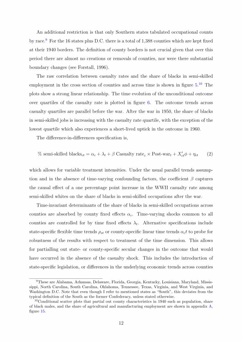
An additional restriction is that only Southern states tabulated occupational counts

by race.9 For the 16 states plus D.C. there is a total of 1,388 counties which are kept fixed

at their 1940 borders. The definition of county borders is not crucial given that over this

period there are almost no creations or removals of counties, nor were there substantial

boundary changes (see Forstall, 1996).

The raw correlation between casualty rates and the share of blacks in semi-skilled

employment in the cross section of counties and across time is shown in figure 5.10 The

plots show a strong linear relationship. The time evolution of the unconditional outcome

over quartiles of the casualty rate is plotted in figure 6. The outcome trends across

casualty quartiles are parallel before the war. After the war in 1950, the share of blacks

in semi-skilled jobs is increasing with the casualty rate quartile, with the exception of the

lowest quartile which also experiences a short-lived uptick in the outcome in 1960.

The difference-in-differences specification is,

% semi-skilled blacksct = αc + λt + β Casualty ratec × Post-wart +X ′ctφ+ ηct (2)

which allows for variable treatment intensities. Under the usual parallel trends assump-

tion and in the absence of time-varying confounding factors, the coefficient β captures

the causal effect of a one percentage point increase in the WWII casualty rate among

semi-skilled whites on the share of blacks in semi-skilled occupations after the war.

Time-invariant determinants of the share of blacks in semi-skilled occupations across

counties are absorbed by county fixed effects αc. Time-varying shocks common to all

counties are controlled for by time fixed effects λt. Alternative specifications include

state-specific flexible time trends ρst or county-specific linear time trends αct to probe for

robustness of the results with respect to treatment of the time dimension. This allows

for partialling out state- or county-specific secular changes in the outcome that would

have occurred in the absence of the casualty shock. This includes the introduction of

state-specific legislation, or differences in the underlying economic trends across counties

9These are Alabama, Arkansas, Delaware, Florida, Georgia, Kentucky, Louisiana, Maryland, Missis-sippi, North Carolina, South Carolina, Oklahoma, Tennessee, Texas, Virginia, and West Virginia, andWashington D.C. Note that even though I refer to mentioned states as “South”, this deviates from thetypical definition of the South as the former Confederacy, unless stated otherwise.

10Conditional scatter plots that partial out county characteristics in 1940 such as population, shareof black males, and the share of agricultural and manufacturing employment are shown in appendix A,figure 15.

12

that are not captured by the controls.

The vector Xct contains controls that seek to capture other potential changes in ob-

servables that might determine the share of blacks in semi-skilled jobs and which correlate

with the casualty rate among semi-skilled whites. The draft rate accounts for the remain-

ing workforce during the war as well as for the share of the male population under threat

of being killed in the war. It also provides an estimate of the male population eligible

for benefits under the G.I. Bill after the war (Turner and Bound, 2003). To account for

spillover effects, I include the average casualty rate in the adjacent counties of a given

county c. The log of WWII related spending per capita captures governmental spending

as potential stimulus to the local economies (see Fishback and Cullen, 2013). Data for

WWII expenditure comes from the County and City Data Book 1947 published by the

U.S. Department of Commerce (2012).

Demographic and political controls include the share of rural population and the share

of black men from the Census, and the Republican vote share from data by Clubb et al.

(2006). To control for factors specific to blacks in the South, the number of lynchings

between 1900 and 1930 per 1,000 blacks, and the number of slaves in 1860 (both interacted

with decade fixed effects) are included. Lynchings had a significant effect on economic

growth generated by black inventors (Cook, 2014). I also include the number of Rosenwald

schools per 1,000 blacks, which are significant determinants of black education (Aaronson

and Mazumder, 2011) and the share of acres flooded by the Mississippi in 1928 interacted

with time as a major shock to internal migration of blacks (Hornbeck and Naidu, 2014).

Given that the manufacturing sector at the time was the main employer of operatives

and craftsmen, I also include the number of manufacturing establishments per capita, the

average firm size measured as the average number of employees per establishment, the

log value added per manufacturing worker as measure for productivity, and the share of

employment in manufacturing in a given county.

Agriculture was a major employer for black workers before the war, hence I include

variables to rule out that shocks related to agricultural productivity or capital accumu-

lation were driving the shift of blacks to semi-skilled employment. These include the

share of land used for agricultural production, the share of acres in cotton, the share of

cash tenants as measure for skill available in the agricultural sector that might have been

portable to semi-skilled employment, and the average value of machinery per farm. The

13

latter seeks to control for technological changes in the agricultural sector. In particular,

the use and quality of tractors expanded at the time, especially in the South and released

labor from the farms (see Olmstead and Rhode, 2001).

Finally, to account for the major economic changes brought by the Great Depression

in the decade just prior to the war, I include measures of New Deal spending per capita

from Fishback et al. (2006). These were distributed as stimulus packages between 1933

and 1935. This includes government loans, money for public works, funds from the

Agricultural Adjustment Act (AAA), and by the Federal Housing Administration (FHA),

as well as the unemployment rate in 1937. All of these variables are interacted with decade

fixed effects. All monetary values are deflated to 2010 U.S. dollars using the CPI provided

by the Bureau of Labor Statistics.

An overview of all data sources used to compile the final estimation sample is given in

the data appendix. Summary statistics are reported in table 2. All remaining variation in

the outcome which is not captured by the previously mentioned right-hand side variables

is absorbed in the error term ηct. Standard errors are clustered at the county level to

account for heteroscedasticity and autocorrelation.

3.2.1 Difference-in-Differences Results

The main results from the estimation of eq. (2) are reported in table 3 under different

model specifications. The effect of a one percentage point increase in the WWII casualty

rate among semi-skilled whites on the county share of blacks in semi-skilled occupations

is between 0.51 and 0.64 p.p. This effect is significant at the one percent level across all

specifications. For an average casualty rate of 3.13% the average effect size thus ranges

between 1.6 to 2 p.p. Given the average share of blacks in this skill group in 1940, a

β × 3.13 p.p. addition corresponds to an increase of 12.9 to 16.1% relative to the pre-

war mean. A recent study by Miller (2017) assesses the affirmative action policies under

President Johnson in 1965. Affected firms increased their share of black employees by 0.8

p.p. five years after. While the magnitudes are not directly comparable due to differences

in sample composition and measurement of variables, it gives context to the effect sizes

estimated here.

There was a similar order by President Roosevelt during the war which established

the Fair Employment Practice Committee (FEPC). Collins (2001) analyzed its role in the

14

employment of blacks in war related industries. Even though he finds significant effects

in the North, he also notes that the FEPC was ineffective in the South due to a lack of

cooperation by local authorities. While I do not have measures of the FEPC’s effective-

ness, the results here are unlikely to be driven by the affirmative action policies under

Roosevelt. The FEPC disbanded shortly after the war and new employment policies of

this type did not come into effect until the Civil Rights Act of 1964.

Inclusion of the controls does not alter the results in column (2). A potential concern

is that some of these controls could themselves be outcomes of the casualty rate, such as

the share of manufacturing employment or the share of blacks in a county. To alleviate

these concerns, I fix all controls at their pre-war levels in 1940 and interact them with

decade fixed effects in column (3). Again the results remain unchanged. Columns (4)

and (5) present specifications with flexible state-specific time trends and county-specific

linear time trends, respectively, to absorb secular trends in the outcome over time that

might otherwise be picked up by the casualty rate.

The final column reports estimates using the doubly-robust selection procedure by

Belloni et al. (2014). Their machine learning covariate selection algorithm tests for the

stability of treatment effects and potentially improves inference on such parameters. Sup-

pose that a large set of observed controls includes the most relevant covariates to explain

the relation of interest but that these variables are unknown to the econometrician.11 In

a first step, the outcome is regressed on the controls, their squares, and all cross-term

interactions, after which the most significant predictors are selected either via LASSO

or a simple t-test from a multiple regression if the sample size permits. Here a t-test

sufficed. The same is repeated for the treatment, i.e. the casualty rate in this case. In

a final step, eq. (2) is re-estimated using the union of controls selected in either of the

previous two steps. The idea is that the regression learns the most important predictors

of outcome and treatment which would be problematic omitted variables.

To probe for the sensitivity of the previous results with respect to the unobservable

components, table 3 reports the coefficient sensitivity test by Oster (2017) for all specifi-

cations. She considers a standard linear regression model Y = βX +W1 +W2 + ε, where

W1 = Ψwo is a vector of observable controls and W2 is an index of unobservables. The

treatment variable X here is the casualty rate. She then defines the selection relationship

11These most influential explanatory variables potentially include interactions and squared terms.

15

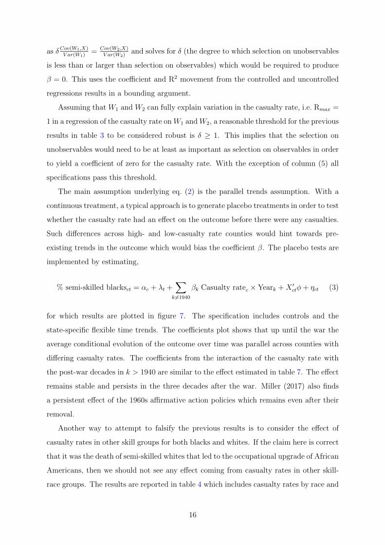
as δCov(W1,X)V ar(W1)

= Cov(W2,X)V ar(W2)

and solves for δ (the degree to which selection on unobservables

is less than or larger than selection on observables) which would be required to produce

β = 0. This uses the coefficient and R2 movement from the controlled and uncontrolled

regressions results in a bounding argument.

Assuming that W1 and W2 can fully explain variation in the casualty rate, i.e. Rmax =

1 in a regression of the casualty rate on W1 andW2, a reasonable threshold for the previous

results in table 3 to be considered robust is δ ≥ 1. This implies that the selection on

unobservables would need to be at least as important as selection on observables in order

to yield a coefficient of zero for the casualty rate. With the exception of column (5) all

specifications pass this threshold.

The main assumption underlying eq. (2) is the parallel trends assumption. With a

continuous treatment, a typical approach is to generate placebo treatments in order to test

whether the casualty rate had an effect on the outcome before there were any casualties.

Such differences across high- and low-casualty rate counties would hint towards pre-

existing trends in the outcome which would bias the coefficient β. The placebo tests are

implemented by estimating,

% semi-skilled blacksct = αc + λt +∑

k 6=1940

βk Casualty ratec × Yeark +X ′ctφ+ ηct (3)

for which results are plotted in figure 7. The specification includes controls and the

state-specific flexible time trends. The coefficients plot shows that up until the war the

average conditional evolution of the outcome over time was parallel across counties with

differing casualty rates. The coefficients from the interaction of the casualty rate with

the post-war decades in k > 1940 are similar to the effect estimated in table 7. The effect

remains stable and persists in the three decades after the war. Miller (2017) also finds

a persistent effect of the 1960s affirmative action policies which remains even after their

removal.

Another way to attempt to falsify the previous results is to consider the effect of

casualty rates in other skill groups for both blacks and whites. If the claim here is correct

that it was the death of semi-skilled whites that led to the occupational upgrade of African

Americans, then we should not see any effect coming from casualty rates in other skill-

race groups. The results are reported in table 4 which includes casualty rates by race and

16

skill group in the regression. The estimated coefficients for the semi-skilled white casualty

rate are not significantly different from what was estimated in the baseline specification.

There is no detectable effect for the casualty rates among low- and high-skilled whites.

Likewise, casualty rates for semi- and high-skilled blacks do not have a significant

impact on the outcome. However, there is a smaller but significant negative effect coming

from the group of low-skilled blacks. A percentage point increase in the casualty rate for

this group decreases the share of semi-skilled blacks by 0.09 to 0.15 p.p. This result is

intuitive given that these are the workers who, had they survived, would have replaced

the deceased semi-skilled whites after the war.12

3.3 Further Evidence from Individual Census Data

The previous results show that the occupational upgrading of blacks also occured in

the South and was not merely a phenomenon driven by the Great Migration. Yet it is

also insightful to generalize the result to the entire country. Doing so requires to assign

casualty rates at the commuting zone level instead of the county level. Commuting zones

are clusters of counties that share a common labor market. There are 722 commuting

zones which can be consistently constructed using the spatial information available in

the individual level data of the 1920 to 1970 U.S. Census files by Ruggles et al. (2018).13

Figure 8 plots the WWII casualty rate among semi-skilled whites at the commuting zone

level.

I use the 1% micro Census files from 1920 to 1950, the 5% file of 1960, and the 1%

form metro sample of 1970. The estimation sample includes the non-institutionalized

working age (16-65) male population who were participating in the labor force at the

enumeration date, who were not enrolled in school or classified as unpaid family workers,

and whose ethnicity was classified as black or white. The micro level data provide the

advantage of using whites an additional control group. If casualties resulted in a labor

supply shock only, then one would expect occupational upgrading to occur for both blacks

and whites. However, if semi-skilled professions had higher barriers to entry for blacks

12All further robustness and sensitivity analyses are reported in appendix A, including further spec-ification tests of the parallel trends assumption, selective migration of blacks, selection on observables,selection of soldiers into the military and into death, alternative treatment and outcome denominators,sensitivity of the results by state, and spatial clustering of the casualty rates.

13The crosswalks for 1950 and 1970 are available on David Dorn’s website (http://www.ddorn.net/data.htm), and the crosswalk files for the other years were kindly shared by Felix Konig.

17

that were removed due to the labor shortages induced by the casualties, then only blacks

should see an effect on their probability to be employed in such jobs.

In the following triple difference (DDD) regression I compare the probability of semi-

skilled employment between blacks and whites, before and after the war, and across

commuting zones with differing casualty rates:

Pr (semi-skilled = 1)izt = β1 (casualty ratez × post-WWIIt)

+ β2 (casualty ratez × blackizt × post-WWIIt)

+ αz + λt + δblackizt +X ′iztγ + εizt (4)

where i, z, and t index individuals, commuting zones, and Census years, respectively. The

outcome is an indicator for whether an individual is a semi-skilled worker (craftsman or

operative). The coefficients of interest are β1 for whites and the triple interaction coeffi-

cient β2 for blacks. Controls include age, marital status, year of birth, a self-employment

indicator, farm status, and industry fixed effects, and αz and λt are commuting zone and

time fixed effects. Standard errors are clustered at the commuting zone level.

The triple differences regression seeks to eliminate potentially confounding trends in

the employment probability of blacks in semi-skilled jobs across commuting zones that

are unrelated to the war casualties. It also accounts for changes in the employment

probability of all workers in high-casualty commuting zones which might have happened

due to other shocks that occurred at the same time. Compared to the county level

regressions, this framework also allows to estimate the casualty rate effect on i) whites,

and ii) on blacks and whites in different industries for the entire U.S.

To visualize the relationship, I interact the casualty ratez and casualty ratez×blackizt

variables with Census year fixed effects in eq. (4), leaving out 1940 as baseline. The

resulting coefficients for blacks and whites are plotted in figure 9. There is no significant

casualty rate effect before the war for either group and remains insignificant for whites

also in the post-war period. This means that there are no differential pre-trends for

blacks or whites across high- and low-casualty rate commuting zones. For blacks there is

a positive post-war effect starting from 1950 which increases over time and peaks in 1970

with a 5 p.p. rise in the semi-skilled employment probability for every one percentage

point increase in the commuting zone WWII casualty rate among semi-skilled whites.

18

Table 5 reports results from estimating eq. (4) for different model specifications. The

triple difference coefficient for black workers is positive and significant in all specifications

and ranges between 1.9 to 4.7 p.p. for the whole country and between 1.1 and 3 p.p.

for workers in the South. There is no effect on whites with the exception of column

(6) where the regression with commuting zone specific time trends shows a small but

negative and significant effect for white workers. The null effect on whites is coherent

with the historic account by Wolfbein (1947): “the movement of [black] men and women

to factories, primarily as semiskilled operatives, was even more pronounced than that of

white persons” (p. 665).

The results show that the employment gains for blacks not only occurred in the North

or West of the country but that also Southern blacks gained significantly in terms of the

occupational upgrading. Another advantage of the micro data is that I can further deal

with potential migration responses. I therefore interact an indicator for whether an

individual lives outside their state of birth with time fixed effects and the black indicator

in column (4). The same interactions are applied to the education variable. The results

show that even though the coefficients are smaller, they are still positive and significant.

It should be noted that migration and education are potential outcomes of the treatment,

hence results from this specification are to be taken with caution. Yet it sheds light on

whether the occupational upgrading effect can be explained away by differential migration

or educational attainment across black and white workers over time.

Next, I analyze whether the occupational upgrading of blacks is concentrated in par-

ticular sectors. Table 6 repeats the analysis for the manufacturing sector as a whole, and

for the durable and non-durable manufacturing sub-sectors, as well as for telecommuni-

cations, retail, and public administration as placebo groups. Unlike the manufacturing

sectors, the jobs in the placebo sectors often involved direct customer contact and there-

fore employers sought to avoid employment of blacks in such positions (Anderson, 1982).

Given that these sectors remained segregated throughout and after the war, they should

not show any occupational gains made by blacks. The results provide evidence that black

occupational upgrading was particularly pronounced in all manufacturing sectors with a

9 to 11 p.p. increase in the probability of semi-skilled employment for blacks for a one

percentage points increase in the WWII casualty rate among semi-skilled whites. Except

for a slight negative effect in retail, there is no effect on blacks in the high-skilled sectors

19

and for whites the effect is never significant in any sector.

4 The Relation between World War II and African American

Economic Progress in the Post-War Era

Several scholars have studied black economic progress at mid-century with respect to

wages (Margo, 1995; Maloney, 1994), cross-state migration (Boustan, 2016) and urban-

ization (Boustan, 2010), home ownership (Collins and Margo, 2011; Boustan and Margo,

2013; Logan and Parman, 2017), or education (Smith, 1984). If African Americans made

progress on all these dimensions and at the same time, then it is likely that there exists at

least one underlying common factor. Both Maloney (1995) and Margo (1995) discussed

the labor shortages during the war as potential reason for the wage gains made by black

workers. According to Margo (1995, p. 472), “the most important example of occupa-

tional upgrading was the increase of blacks in semi-skilled operative positions. Such jobs

paid far better than farm labor [...] that blacks were accustomed to”.

I next study the war, and in particular the role of semi-skilled white casualty rates

as driver of the black occupational upgrade, as common denominator for the post-war

progress made by blacks on other economic dimensions analyzed in prior work.14 I again

use the individual level data from the Census between 1920 and 1970 from the previous

section. To test the hypothesis that other economic improvements for blacks are related

to the war, I re-run eq. (4),

yizt = β1 (casualty ratez × post-WWIIt)

+ β2 (casualty ratez × blackizt × post-WWIIt)

+ αz + λt + δblackizt +X ′iztγ + εizt (5)

with different economic outcomes yizt which are the log of an individual’s real annual

wage, years of completed education, an indicator for whether they own their home, the

log house value, and an indicator for whether a person’s state of residence is not their

state of birth. Results for the full sample and for the Southern subsample are reported

in panels A and B in table 7, respectively. The corresponding dynamic coefficient plots

14Appendix B performs this analysis using semi-skilled employment as treatment for comparisonpurposes. The casualty rate is the more exogenous variable and hence was preferred for the mainspecification.

20

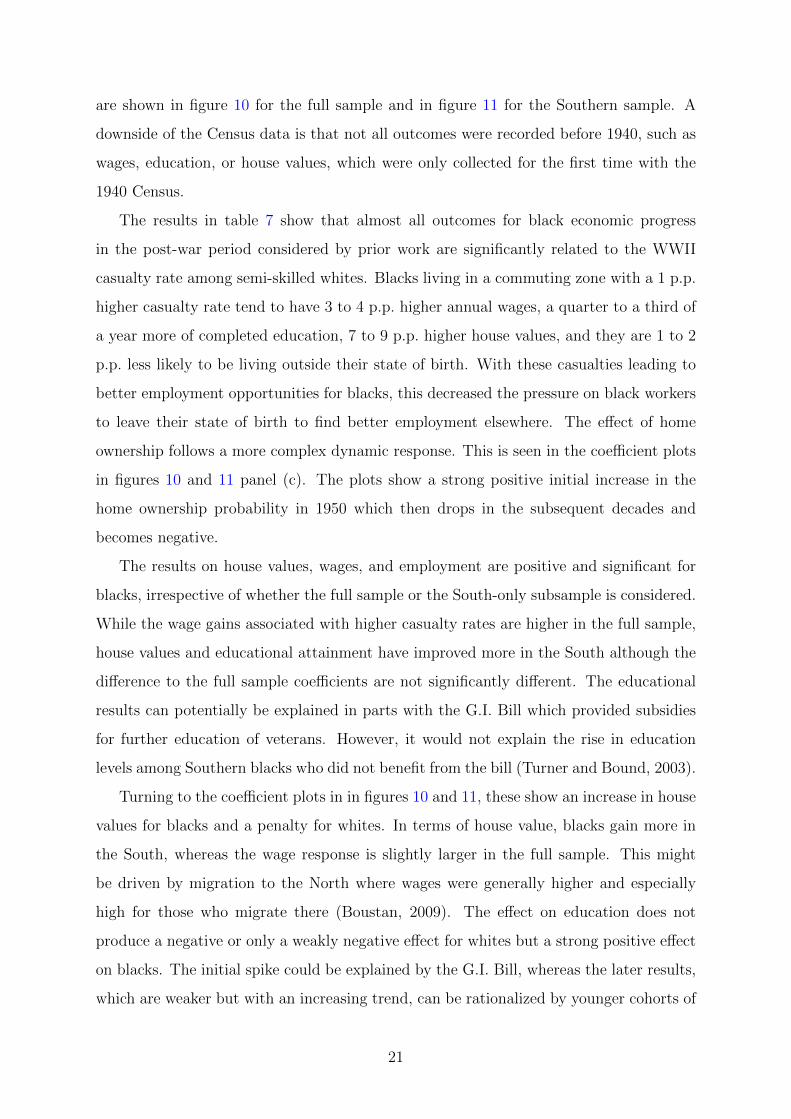
are shown in figure 10 for the full sample and in figure 11 for the Southern sample. A

downside of the Census data is that not all outcomes were recorded before 1940, such as

wages, education, or house values, which were only collected for the first time with the

1940 Census.

The results in table 7 show that almost all outcomes for black economic progress

in the post-war period considered by prior work are significantly related to the WWII

casualty rate among semi-skilled whites. Blacks living in a commuting zone with a 1 p.p.

higher casualty rate tend to have 3 to 4 p.p. higher annual wages, a quarter to a third of

a year more of completed education, 7 to 9 p.p. higher house values, and they are 1 to 2

p.p. less likely to be living outside their state of birth. With these casualties leading to

better employment opportunities for blacks, this decreased the pressure on black workers

to leave their state of birth to find better employment elsewhere. The effect of home

ownership follows a more complex dynamic response. This is seen in the coefficient plots

in figures 10 and 11 panel (c). The plots show a strong positive initial increase in the

home ownership probability in 1950 which then drops in the subsequent decades and

becomes negative.

The results on house values, wages, and employment are positive and significant for

blacks, irrespective of whether the full sample or the South-only subsample is considered.

While the wage gains associated with higher casualty rates are higher in the full sample,

house values and educational attainment have improved more in the South although the

difference to the full sample coefficients are not significantly different. The educational

results can potentially be explained in parts with the G.I. Bill which provided subsidies

for further education of veterans. However, it would not explain the rise in education

levels among Southern blacks who did not benefit from the bill (Turner and Bound, 2003).

Turning to the coefficient plots in in figures 10 and 11, these show an increase in house

values for blacks and a penalty for whites. In terms of house value, blacks gain more in

the South, whereas the wage response is slightly larger in the full sample. This might

be driven by migration to the North where wages were generally higher and especially

high for those who migrate there (Boustan, 2009). The effect on education does not

produce a negative or only a weakly negative effect for whites but a strong positive effect

on blacks. The initial spike could be explained by the G.I. Bill, whereas the later results,

which are weaker but with an increasing trend, can be rationalized by younger cohorts of

21

African Americans. The wartime cohort basically showed that semi-skilled employment

is now within reach for blacks, meaning that the benefits of acquiring more education

before entering the labor market were more tangible to the newer cohorts. The coefficient

plots in figures 10 and 11 reveal that any negative effect on whites is short-lived and zero

otherwise. The wage coefficients display a strong upward trend for blacks, especially in

1970 when the Civil Rights Act of 1964 likely reinforced the wage effect.

5 Black Occupational Upgrading and Black-White Social Rela-

tions in the South in 1961

The war elevated African American’s economic position by providing them with access

to better-paid semi-skilled jobs, especially in the manufacturing sector. During the war,

this was not always embraced by white workers. In 1944, the Philadelphia Transportation

Company began to alleviate labor shortages by allowing blacks to enter semi-skilled oc-

cupations. White workers initiated a strike which was broken when the Army threatened

to re-evaluate the draft deferments of striking workers (Collins, 2001). As with the Civil

Rights movement, it took some time for whites to adapt to the new workplace realities

(see Wright, 2013). What was the longer-term effect of the casualty-induced economic

upgrading of blacks on their social status and their relationship with whites?

The answer to this question is not obvious a priori. A well-established concept in the

study of network formation is homophily whereby individuals prefer contact with other

agents who are more like themselves in terms of age, race, income, and other characteris-

tics (see Currarini et al., 2009). As the economic position of African Americans improved

during and after the war, they became more similar to whites in economic characteristics

and therefore their relations may have improved. However, if whites perceived blacks as

economic rivals, such as in the case of the Philadelphia Transport Company, the exact

opposite could have happened.

To study the above question, I use the “Negro Political Participation Study” (NPPS)

of 1961 by Matthews and Prothro (1975). The study was conducted in states of the

former Confederacy for a random sample of 540 black and 528 white adults in 1961. For

the analysis I coded responses to questions regarding the social integration and status of

blacks into binary variables.15 The outcomes are interracial friendships, living in mixed-

15Social integration here refers to any question concerning non-market interactions between blacks

22

race neighborhoods, and attitudes towards integration of respondents and their church

ministers. A complete list of the specific questions and the coding scheme for the outcome

variables is provided in table 8. The summary statistics are reported in table 9.

Despite the relatively small sample size, this data set provides a unique opportunity to

study the social standing of African Americans in the South before the riots and violence

between 1963 and 1970, and before the major legislative and legal reforms against segre-

gation were passed and implemented. Major desegregation laws, such as the Civil Rights

Act of 1964, the Voting Rights Act of 1965, the Fair Housing Act of 1968, or Supreme

Court rulings such as Loving vs. Virginia 1967, which invalidated anti-miscegenation

laws, were only enacted later. The only exception is the Supreme Court case of Brown

vs. Board of Education of Topeka in 1954 wherein segregation at public schools was de-

clared unconstitutional. However, it took more than a decade to be fully implemented

(Wright, 2013).

5.1 Model Specification and Results

Regressing outcomes related to black-white social interaction and attitudes on the

share of blacks in semi-skilled occupations as in,

social outcomeic = β∆share of blacksc + α share of blacksc,1940 +X ′icδ + εic (6)

where i and c index individuals and counties, respectively, and where social outcomes

are the ones described in table 8, may not provide unbiased and consistent estimates. A

potential issue is reverse causality. The regression in eq. (6) assumes that an individual’s

economic status affects her social status. The opposite might be true when better job

opportunities arise from an increase in social contacts. To address this type of endogeneity

problem, I instrument the change in the share of blacks in semi-skilled jobs from 1940 to

1950 (∆share of blacksc) with the WWII casualty rate among semi-skilled whites:

∆share of blacksc = φcasualty ratec + π share of blacksc,1940 +X ′icγ + ρc (7)

The casualty rate is defined as before, ρc and εic are stochastic error terms, and X ′ic is a

and whites, or attitudes towards people from the opposite race.

23

vector of individual and county level controls as well as state fixed effects. Controlling

for the pre-war level of the share of blacks in semi-skilled jobs accounts for cross-county

level differences in market-based discrimination before. For a given level of blacks in this

skill group, ∆share of blacksc then provides the additional inflow of blacks into this skill

group during the war years. The effect of this inflow might have a different impact when

starting from a low or high pre-war level. This simply is a way to leverage the time

information on the treatment in cross sectional survey data.

The main assumptions required for identification are that the casualty rate is a suffi-

ciently relevant predictor of ∆share of blacksc and that it does not correlate with the error

term of a given social outcome. A threat to identification would be joint service of blacks

and whites in the war. Draft and casualty rates correlate positively. Serving together

in battle could have created bonds between black and white soldiers. If those translated

to better social relations in the workplace because of their common war experience, this

would violate the exclusion restriction. To alleviate such concerns, all regressions control

for a respondent’s veteran status and the county draft rate.

Further controls that are potential determinants of interracial social relations and that

might correlate with semi-skilled employment include gender, age, race, the county an

individual grew up in, the number of years an individual has spent in their current county

of residence, and place size. Additional county level controls include the percentage of

blacks, the share of people born in other counties, the WWII draft rate, the number of

lynchings between 1900 and 1930, and the number of Rosenwald schools per 1,000 blacks,

as well as the number of slaves in 1860.

Another important control is the location of a respondent’s dwelling (rural, rural non-

farm, suburban, and urban). Boustan (2010, 2016) shows that in-migration of blacks to

the centers of Northern cities led whites to move to the periphery. This phenomenon is

known in the literature as white flight. If unaccounted for, blacks would find semi-skilled

occupations in the city centers and make friends with whites though not because of their

improved economic position but because all the whites who had a distaste for interactions

with blacks moved to the suburbs. Summary statistics for the individual level controls

by race are reported in table 10.

A significant shortcoming of this data set is that these individuals cluster in only

24 different counties. This is mainly an inference problem due to the sampling scheme

24

employed. First, primary sampling units (counties or collections of counties) were drawn

at random within each Southern state, then individuals were sampled from within a

chosen area. The data are therefore representative of the Southern population as ar-

gued by Matthews and Prothro (1975). The sample counties are mapped in figure

12. Nevertheless, 24 clusters are not enough for the conventionally used cluster-robust

variance-covariance estimator to be consistent as it relies on large sample asymptotics.

Cluster-robust standard errors are reported in parentheses for purposes of comparison.

The standard errors in squared brackets are estimated via the wild cluster bootstrap

t-percentile procedure by Cameron et al. (2008) for the OLS models, and via the wild

restricted efficient residual bootstrap for IV models by Davidson and MacKinnon (2010).

These correct inference for the smaller number of clusters.

OLS and IV results for the regression equation in eq. (6) are reported in table 11. The

sample size is kept constant for all regressions using information from the 540 black and

528 white respondents. The first stage F-statistic on the instrument is sufficiently large

with a value of 43.8. I also report the efficient F-statistic by Olea and Pflueger (2013),

which is robust to heteroscedasticity and clustering, with a value of 45.8. Most of the

IV results are similar to the OLS estimates and show a significant and positive effect of

the black skill-upgrade on social relations between blacks and whites. Issues related to

omitted variables or selection appear to be less relevant in the context of these outcomes.

A casualty-induced one percentage point increase in ∆share of blacksc is associated

with an 1.8 p.p. increase in a respondent’s probability of reporting an interracial friend-

ship. The OLS and IV estimates are virtually the same. An increase in the share of

blacks in semi-skilled jobs at the average casualty rate thus increases this probability by

2.9 p.p.16 Camargo et al. (2010) show that white students who were randomly assigned a

black roommate in their first year of college had a 10.5 p.p. higher probability of having

an interracial friendship in the second year. Compared to their estimates, the friendship

effect at the average casualty rate is abut 28% of the exposure treatment for college stu-

dents in the early 2000s. This seems reasonable and puts the magnitude of the estimated

coefficients into perspective.

Respondents in treated counties stated with a 1.2 p.p. higher probability that they

16Section 3.2.1 estimated an increase in the share of blacks in semiskilled jobs of 0.515 for a 1 p.p.increase in the casualty rate. Since the regression includes fixed effects, this will be similar to a regressionin first differences using ∆share of blacksc as outcome. Hence the friendship effect at an average casualtyrate is 3.1× 0.515× 1.8 = 2.87.

25

lived in mixed-race areas. Relative to the outcome mean of 12.4% this is a sizable effect.

Given that the share of blacks in the county and dwelling location are controlled for,

this is not a mere population composition effect but must have been an active choice

by respondents. The black occupational upgrade also had significant effects on attitudes

towards integration. Each percentage point increase in ∆share of blacksc is associated

with a 1 p.p. higher probability of respondents favoring integrating in the OLS and 2 p.p.

higher in the IV estimation.

Breaking this down further, support for integration at school increased by 1 p.p. and

by 0.3 (OLS) and 0.8 (IV) p.p. for integration at church. Favoring interracial exposure of

their children or in their churches provides significant evidence for the extent of the effects

of the improved economic position of blacks on black-white social relations. The results

relating to integration at church indicate a willingness to accept the other racial group

into the most intimate spheres of social life. Even nowadays there is a strong racial divide

in church memberships and service, and Martin Luther King stated in several speeches

that 11 o’clock on Sunday is the most segregated hour in American life (see Fryer, 2007).

There also appears to be an institutional component since respondents in treated counties

were 0.5 to 1.5 p.p. less likely to report their ministers preaching in favor of segregation.

However, given the data it is not possible to say whether this was a demand or supply

effect. Individuals with higher interracial exposure or contacts might have demanded less

segregationist priests, while another possibility is that such priests were predominantly

assigned to areas were racial tensions were lower.

The results suggest that the casualty-induced skill-upgrade of African Americans not

only came with a rise in economic but also in social status.17

6 Conclusion

Much has changed since Myrdal’s (1944) negative assessment of the economic and

social fortunes of African Americans. This is particularly true for the middle of the last

century. While writing his book, Myrdal had recognized the importance of the war for

17Appendix C provides further heterogeneity analyses by repeating the estimation for the black andwhite sub-samples, as well as robustness checks with respect to weighting blacks by their populationshare in the county, changing the definition of the treatment variable, and to assess sensitivity of the IVestimates with respect to mild violations of the exclusion restriction. It also provides a causal mediationanalysis to see whether higher incomes for blacks are a mechanism that mediates the effects found in themain analysis.

26

the employment of blacks: “The present War is of tremendous importance to the Negro

in all respects. He has seen his strategic position strengthened not only because of the

desperate scarcity of labor but also because of a revitalization of the American Creed.”

(1944, p. 409). This paper shows that this scarcity was particularly pronounced in areas

with higher WWII casualty rates among semi-skilled whites. These losses opened up

new employment opportunities for blacks and contributed to the largest occupational

upgrading of African Americans since the end of the Civil War.

Understanding the roots of this unprecedented occupational gain helps to understand

African American progress at mid-century. While some path breaking work has assessed

black economic progress at mid-century with respect to wages (Margo, 1995; Maloney,

1994; Bailey and Collins, 2006), migration and urbanization (Boustan, 2009, 2010, 2016),

home ownership (Collins and Margo, 2011; Boustan and Margo, 2013; Logan and Parman,

2017), or education (Smith, 1984; Turner and Bound, 2003), our knowledge of the origins

of the sudden and strong improvements during and after the war has been limited. The

analysis here provides evidence that several of the economic outcomes considered by

previous work can be directly related to the war. In particular, they relate to the casualty

rate among semi-skilled whites as driver of the black occupational upgrade. I rule out

alternative explanations for this pattern based on migration or increased educational

attainment by blacks.

The improvements in the position of blacks go beyond the economic gains. The

survey data results provide some insights which indicate that areas with a larger wartime

upgrading of blacks into semi-skilled employment also saw a rise in their social status.

This ranges from increased interracial friendships to higher acceptance of the other group

at school or church. The economic upgrading of a minority group thus has the potential

to even affect strongly embedded social values in a conservative setting such as the Bible

Belt in the early 1960s.

Even though this paper has quantified the relationships between the war casualties

and the occupational upgrade, as well as the economic and social outcomes of blacks,

it remained mostly silent on the specific mechanisms behind these relationships. The

difficulty is to determine which variables are outcomes, treatments, or mediators. Several

channels of causation may exist at the same time. The occupational upgrade not only

came with better-paying jobs but also with the opportunity to interact more with white

27

workers in the workplace. Is the improvement in social relations driven by inter-group

contact at work or by the relaxation of black households’ budget constraints that allow

for social activities or for moving to better neighborhoods? Exploring these questions

might offer a promising avenue for future research.

28

References

Aaronson, D. and Mazumder, B. (2011) “The Impact of Rosenwald Schools on Black Achieve-ment”, Journal of Political Economy, Vol. 119(5), pp. 821-888

Acemoglu, D., Autor, D.H., and Lyle, D. (2004) “Women, War, and Wages: The Effect ofFemale Labor Supply on the Wage Structure at Midcentury”, Journal of Political Economy,Vol. 112(3), pp. 497-551

Alesina, A. Baqir, R., and Easterly, W. (1999) “Public Goods and Ethnic Divisions”, QuarterlyJournal of Economics, Vol. 114(4), pp. 1243-1284

Anderson, K.T. (1982) “Last Hired, First Fired: Black Women Workers during World War II”,Journal of American History, Vol. 69(1), pp. 82-97

Bailey, M.J. and Collins, W.J. (2006) “The Wage Gains of African-American Women in the1940s”, Journal of Economic History, Vol. 66(3), pp. 737-777

Bayer, P. and Charles, K.K. (2018) “Divergent Paths: A New Perspective on Earnings Dif-ferences Between Black and White Men Since 1940”, Quarterly Journal of Economics, Vol.133(3), pp. 1459-1501

Belloni, A., Chernozhukov, V., and Hansen, C. (2014) “High-Dimensional Methods and Infer-ence on Structural and Treatment Effects”, Journal of Economic Perspectives, Vol. 28(2),pp. 29-50

Bound, J. and Freeman, R.B. (1992) “What Went Wrong? The Erosion of Relative Earningsand Employment Among Young Black Men in the 1980s”, Quarterly Journal of Economics,Vol. 107(1), pp. 201-232

Boustan, L.P. (2009) “Competition in the Promised Land: Black Migration and Racial WageConvergence in the North, 1940-1970”, Journal of Economic History, Vol. 69(3), pp. 755-782

Boustan, L.P. (2010) “Was Postwar Suburbanization “White Flight”? Evidence from the BlackMigration”, Quarterly Journal of Economics, Vol. 125(1), pp. 417-443

Boustan, L.P. (2016) “Competition in the Promised Land: Black Migrants in Northern Citiesand Labor Markets”, Princeton University Press, Princeton, NJ

Boustan, L.P. and Margo, R.A. (2013) “A silver lining to white flight? White suburbanizationand African-American Homeownership, 1940-1980”, Journal of Urban Economics, Vol. 78November, pp. 71-80

Camargo, B., Stinebrickner, R., and Stinebrickner, T. (2010) “Interracial Friendships in Col-lege”, Journal of Labor Economics, Vol. 28(4), pp. 861-892

Cameron, A.C., Gelbach, J.B., and Miller, D.L. (2008) “Bootstrap-based Improvements forInference with Clustered Errors”, Review of Economics and Statistics, Vol. 90(3), pp. 414-427

Clubb, J.M., Flanigan, W.H., and Zingale, N.H. (2006) “Electoral Data for Counties in theUnited States: Presidential and Congressional Races, 1840-1972”, ICPSR08611-v1. AnnArbor, MI: Inter-university Consortium for Political and Social Research [distributor], 2006-11-13. DOI: https://doi.org/10.3886/ICPSR08611.v1

29

Coate, S. and Loury, G.C. (1993) “Will Affirmative-Action Policies Eliminate Negative Stereo-types?”, American Economic Review, Vol. 83(5), pp. 1220-1240

Collins, W.J. (2000) “African-American Economic Mobility in the 1940s: A Portrait from thePalmer Survey”, Journal of Economic History, Vol. 60(3), pp. 756-781

Collins, W.J. (2001) “Race, Roosevelt, and Wartime Production: Fair Employment in WorldWar II Labor Markets”, American Economic Review, Vol. 91(1), pp. 272-286

Collins, W.J. and Margo, R.A. (2006) “Historical Perspectives on Racial Differences in Schoolingin the United States”, in Hanushek, E. and Welch, F. (eds.) Handbook of the Economics ofEducation, Vol. 1, Ch. 3, pp. 107-154, Elsevier, North Holland, NL

Collins, W.J. and Margo, R.A. (2011) “Race and Home Ownership from the End of the CivilWar to the Present”, American Economic Review P&P, Vol. 101(3), pp. 355-359

Conley, T.G. (1999) “GMM estimation with cross sectional dependence”, Journal of Economet-rics, Vol. 92(1), pp. 1-45

Conley, T.G., Hansen, C.B., and Rossi, P.E. (2012) “Plausibly Exogenous”, Review of Eco-nomics and Statistics, Vol. 94(1), pp. 260-272

Cook, L.D. (2014) “Violence and Economic Activity: Evidence from African American Patents,1870-1940”, Journal of Economic Growth, Vol. 19(2), pp. 221-257

Currarini, S., Jackson, M.O., and Pin, P. (2009) “An Economic Model of Friendship: Homophily,Minorities, and Segregation”, Econometrica, Vol. 77(4), pp. 1003-1045

Davidson, R. and MacKinnon, J.G. (2010) “Wild Bootstrap Tests for IV Regression”, Journalof Business and Economics, Vol. 28(1), pp. 128-144

Dippel, C., Gold, R., Heblich, S., and Pinto, R. (2017) “Instrumental Variables and CausalMechanisms: Unpacking the Effect of Trade on Workers and Voters”, NBER Working PaperNo. 23209

Donohue, J.J. III and Heckman, J. (1991) “Continuous Versus Episodic Change: The Impactof Civil Rights Policy on the Economic Status of Blacks”, Journal of Economic Literature,Vol. 29(4), pp. 1603-1643

Eriksson, K. (2018) “Moving North and into jail? The great migration and black incarceration”,Journal of Economic Behavior and Organization, forthcoming. DOI: https://doi.org/10.1016/j.jebo.2018.04.024

Eriksson, K. and Niemesh, G.T. (2016) “Death in the Promised Land: The Great Migrationand Black Infant Mortality”, mimeo

Fishback, P.V., Horrace, W.C., and Kantor, S. (2006) “The impact of New Deal expenditureson mobility during the Great Depression”, Explorations in Economic History, Vol. 43(2), pp.179-222

Fishback, P.V. and Cullen, J.A. (2013) “Second World War Spending and Local EconomicActivity in U.S. Counties, 1939-58”, Economic History Review, Vol. 66(4), pp. 975-992

Flynn, G.Q. (1993) “The Draft, 1940-1973”, University Press of Kansas, Lawrence, KS

Forstall, R.L. (1996) “Population of States and Counties of the United States: 1790-1990”, U.S.Bureau of the Census, Washington, D.C.

30

Fryer, R.G. Jr. (2007) “Guess Who’s Been Coming to Dinner? Trends in Interracial Marriageover the 20th Century”, Journal of Economic Perspectives, Vol. 21(2), pp. 71-90

Getis, A. and Ord, J.K. (1992) “The Analysis of Spatial Association by Use of Distance Statis-tics”, Geographical Analysis, Vol. 24(3), pp. 189-206

Glass, C. (2013) “Deserter: A Hidden Story of the Second World War”, The Penguin Press,New York, NY

Goldin, C. (1991) “The Role of World War II in the Rise of Women’s Employment”, AmericanEconomic Review, Vol. 81(4), pp. 741-756

Goldin, C. and Margo, R.A. (1992) “The Great Compression: The Wage Structure in the UnitedStates at Mid- Century”, Quarterly Journal of Economics, Vol. 107(1), pp. 1-34

Goldin, C. and Olivetti, C. (2013) “Shocking Labor Supply: A Reassessment of the Role ofWorld War II on Women’s Labor Supply”, American Economic Review P&P, Vol. 103(3),pp. 257-262

Haines, M., Fishback, P.V., and Rhode, P. (2016) “United States Agriculture Data, 1840 - 2012”,Study No. ICPSR35206-v3, Inter-university Consortium for Political and Social Research2016-06-29, Ann Arbor, MI

Hornbeck, R. and Naidu, S. (2014) “When the Levee Breaks: Black Migration and EconomicDevelopment in the American South”, American Economic Review, Vol. 104(3), pp. 963-990

Jaworski, T. (2014) “You’re in the Army Now: The Impact of World War II on Women’sEducation, Work, and Family”, Journal of Economic History, Vol. 74(1), pp. 169-195

Kondo, K. (2016) “Hot and cold spot analysis using Stata”, The Stata Journal, Vol. 16(3), pp.612-631

Kriner, D. and Shen, F.X. (2010) “The Casualty Gap: The Causes and Consequences of Amer-ican Wartime Inequalities”, Oxford University Press, Oxford, UK

Larsen, T.B. (2015) “The Strange Career of Jim Crow: Labor Scarcity and Racial Treatmentin the American South”, mimeo

Lee, U. (1965) “The Employment of Negro Troops”, in Conn, S. (eds.) United States Army inWorld War II, Center of Military History U.S. Army, Washington D.C.

Logan, T.D. and Parman, J.M. (2017) “Segregation and Homeownership in the Early TwentiethCentury”, American Economic Review P&P, Vol. 107(5), pp. 410-414

Maloney, T.N. (1994) “Wage Compression and Wage Inequality Between Black and White Malesin the United States, 1940-1960”, Journal of Economic History, Vol. 54(2), pp. 358-381

Margo, R.A. (1995) “Explaining Black-White Wage Convergence, 1940-1950”, Industrial andLabor Relations Review, Vol. 48(3), pp. 470-481

Matthews, D. and Prothro, J. (1975) “Negro Political Participation Study, 1961-1962”, StudyNo. ICPSR07255-v3, Inter-university Consortium for Political and Social Research 2006-08-15, Ann Arbor, MI

Miller, C. (2017) “The Persistent Effect of Temporary Affirmative Action”, American EconomicJournal: Applied Economics, Vol. 9(3), pp. 152-190

31

Moran, P.A.P. (1950) “Notes on Continuous Stochastic Phenomena”, Biometrika, Vol. 37(1/2),pp. 17-23

Myrdal, G. (1944) “An American Dilemma: The Negro Problem and Modern Democracy”,Harper & Brothers Publishers, New York, NY

Olea, J.L.M. and Pflueger, C. (2013) “A Robust Test for Weak Instruments”, Journal of Businessand Economics, Vol. 31(3), pp. 358-369

Olmstead, A.L. and Rhode, P.W. (2001) “Reshaping the Landscape: The Impact and Diffusionof the Tractor in American Agriculture, 1910-1960”, Journal of Economic History, Vol. 61(3),pp. 663-698

Oster, E. (2017) “Unobservable Selection and Coefficient Stability: Theory and Evidence”,Journal of Business and Economic Statistics, in print. DOI: https://doi.org/10.1080/07350015.2016.1227711

Pei, Z., Pischke, J-S., and Schwandt, H. (2018) “Poorly Measured Confounders are More Usefulon the Left than on the Right”, Journal of Business and Economic Statistics, forthcoming.DOI: https://doi.org/10.1080/07350015.2018.1462710

Ruggles, S., Flood, S., Goeken, R., Grover, J., Meyer, E., Pacas, J., and Sobek, M. (2018)“IPUMS USA”, Version 8.0 [dataset]. Minneapolis, MN: IPUMS, 2018. DOI: https://doi.org/10.18128/D010.V8.0

Shatnawi, D. and Fishback, P.V. (2018) “The Impact of World War II on the Demand forFemale Workers in Manufacturing”, Journal of Economic History, Vol. 78(2), pp. 539-574

Smith, J.P. (1984) “Race and Human Capital”, American Economic Review, Vol. 74(4), pp.685-698

Turner, S. and Bound, J. (2003) “Closing the Gap or Widening the Divide: The Effects of theG.I. Bill and World War II on the Educational Outcomes of Black Americans”, Journal ofEconomic History, Vol. 63(1), pp. 145-177

United States Department of Commerce. Bureau of the Census. “County and City Data Book[United States] Consolidated File: County Data, 1947-1977. ICPSR07736-v2”. Ann Arbor,MI: Inter-university Consortium for Political and Social Research [distributor], 2012-09-18.DOI: https://doi.org/10.3886/ICPSR07736.v2

Wasi, N. and Flaaen, A. (2015) “Record Linkage Using Stata: Preprocessing, Linking, andReviewing Utilities”, The Stata Journal, Vol. 15(3), pp. 672-697

Weaver, R.C. (1945) “Negro Employment in the Aircraft Industry”, Quarterly Journal of Eco-nomics, Vol. 59(4), pp. 597-625

Wolfbein, S.L. (1947) “Postwar trends in Negro employment”, Monthly Labor Review, Dec.1947, pp. 663-665

Wright, G. (2013) “Sharing the Prize”, Harvard University Press, Cambridge, MA

32

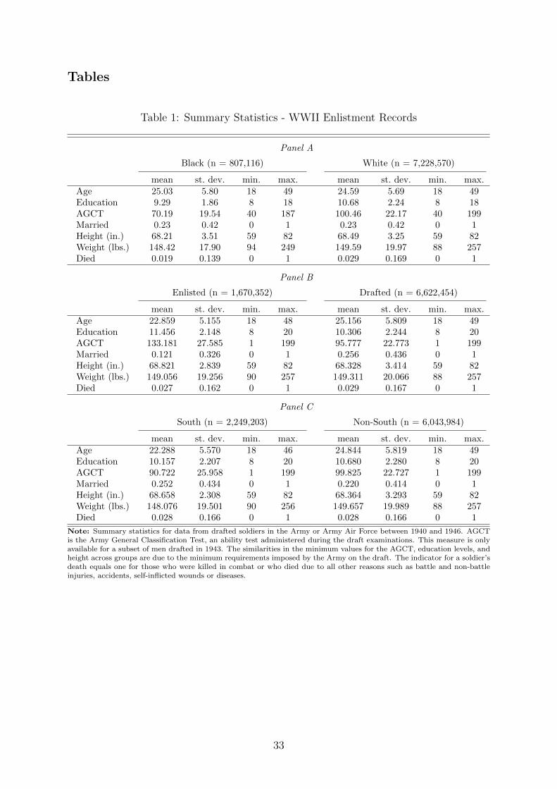
Tables

Table 1: Summary Statistics - WWII Enlistment Records

Panel A

Black (n = 807,116) White (n = 7,228,570)

mean st. dev. min. max. mean st. dev. min. max.Age 25.03 5.80 18 49 24.59 5.69 18 49Education 9.29 1.86 8 18 10.68 2.24 8 18AGCT 70.19 19.54 40 187 100.46 22.17 40 199Married 0.23 0.42 0 1 0.23 0.42 0 1Height (in.) 68.21 3.51 59 82 68.49 3.25 59 82Weight (lbs.) 148.42 17.90 94 249 149.59 19.97 88 257Died 0.019 0.139 0 1 0.029 0.169 0 1

Panel B

Enlisted (n = 1,670,352) Drafted (n = 6,622,454)

mean st. dev. min. max. mean st. dev. min. max.Age 22.859 5.155 18 48 25.156 5.809 18 49Education 11.456 2.148 8 20 10.306 2.244 8 20AGCT 133.181 27.585 1 199 95.777 22.773 1 199Married 0.121 0.326 0 1 0.256 0.436 0 1Height (in.) 68.821 2.839 59 82 68.328 3.414 59 82Weight (lbs.) 149.056 19.256 90 257 149.311 20.066 88 257Died 0.027 0.162 0 1 0.029 0.167 0 1

Panel C

South (n = 2,249,203) Non-South (n = 6,043,984)

mean st. dev. min. max. mean st. dev. min. max.Age 22.288 5.570 18 46 24.844 5.819 18 49Education 10.157 2.207 8 20 10.680 2.280 8 20AGCT 90.722 25.958 1 199 99.825 22.727 1 199Married 0.252 0.434 0 1 0.220 0.414 0 1Height (in.) 68.658 2.308 59 82 68.364 3.293 59 82Weight (lbs.) 148.076 19.501 90 256 149.657 19.989 88 257Died 0.028 0.166 0 1 0.028 0.166 0 1

Note: Summary statistics for data from drafted soldiers in the Army or Army Air Force between 1940 and 1946. AGCTis the Army General Classification Test, an ability test administered during the draft examinations. This measure is onlyavailable for a subset of men drafted in 1943. The similarities in the minimum values for the AGCT, education levels, andheight across groups are due to the minimum requirements imposed by the Army on the draft. The indicator for a soldier’sdeath equals one for those who were killed in combat or who died due to all other reasons such as battle and non-battleinjuries, accidents, self-inflicted wounds or diseases.

33

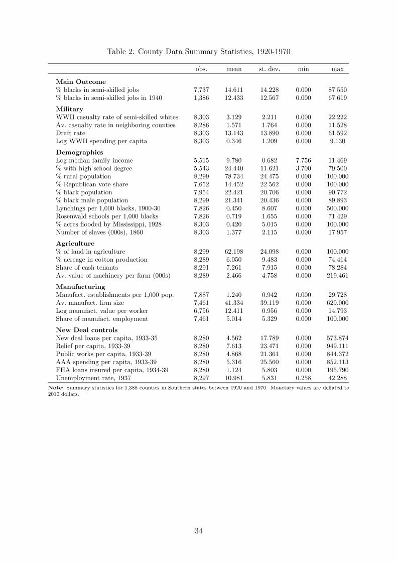
Table 2: County Data Summary Statistics, 1920-1970

obs. mean st. dev. min max

Main Outcome% blacks in semi-skilled jobs 7,737 14.611 14.228 0.000 87.550% blacks in semi-skilled jobs in 1940 1,386 12.433 12.567 0.000 67.619

MilitaryWWII casualty rate of semi-skilled whites 8,303 3.129 2.211 0.000 22.222Av. casualty rate in neighboring counties 8,286 1.571 1.764 0.000 11.528Draft rate 8,303 13.143 13.890 0.000 61.592Log WWII spending per capita 8,303 0.346 1.209 0.000 9.130

DemographicsLog median family income 5,515 9.780 0.682 7.756 11.469% with high school degree 5,543 24.440 11.621 3.700 79.500% rural population 8,299 78.734 24.475 0.000 100.000% Republican vote share 7,652 14.452 22.562 0.000 100.000% black population 7,954 22.421 20.706 0.000 90.772% black male population 8,299 21.341 20.436 0.000 89.893Lynchings per 1,000 blacks, 1900-30 7,826 0.450 8.607 0.000 500.000Rosenwald schools per 1,000 blacks 7,826 0.719 1.655 0.000 71.429% acres flooded by Mississippi, 1928 8,303 0.420 5.015 0.000 100.000Number of slaves (000s), 1860 8,303 1.377 2.115 0.000 17.957

Agriculture% of land in agriculture 8,299 62.198 24.098 0.000 100.000% acreage in cotton production 8,289 6.050 9.483 0.000 74.414Share of cash tenants 8,291 7.261 7.915 0.000 78.284Av. value of machinery per farm (000s) 8,289 2.466 4.758 0.000 219.461

ManufacturingManufact. establishments per 1,000 pop. 7,887 1.240 0.942 0.000 29.728Av. manufact. firm size 7,461 41.334 39.119 0.000 629.000Log manufact. value per worker 6,756 12.411 0.956 0.000 14.793Share of manufact. employment 7,461 5.014 5.329 0.000 100.000

New Deal controlsNew deal loans per capita, 1933-35 8,280 4.562 17.789 0.000 573.874Relief per capita, 1933-39 8,280 7.613 23.471 0.000 949.111Public works per capita, 1933-39 8,280 4.868 21.361 0.000 844.372AAA spending per capita, 1933-39 8,280 5.316 25.560 0.000 852.113FHA loans insured per capita, 1934-39 8,280 1.124 5.803 0.000 195.790Unemployment rate, 1937 8,297 10.981 5.831 0.258 42.288

Note: Summary statistics for 1,388 counties in Southern states between 1920 and 1970. Monetary values are deflated to2010 dollars.

34

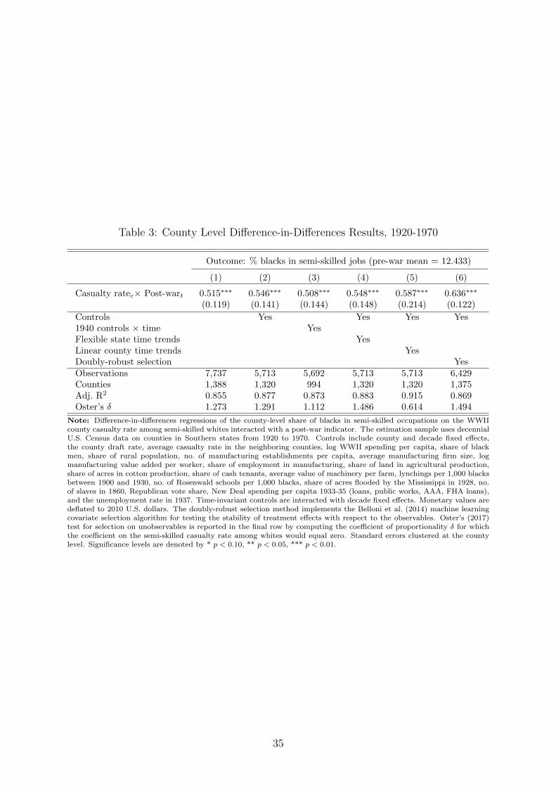
Table 3: County Level Difference-in-Differences Results, 1920-1970

Outcome: % blacks in semi-skilled jobs (pre-war mean = 12.433)

(1) (2) (3) (4) (5) (6)

Casualty ratec× Post-wart 0.515∗∗∗ 0.546∗∗∗ 0.508∗∗∗ 0.548∗∗∗ 0.587∗∗∗ 0.636∗∗∗

(0.119) (0.141) (0.144) (0.148) (0.214) (0.122)

Controls Yes Yes Yes Yes1940 controls × time YesFlexible state time trends YesLinear county time trends YesDoubly-robust selection YesObservations 7,737 5,713 5,692 5,713 5,713 6,429Counties 1,388 1,320 994 1,320 1,320 1,375Adj. R2 0.855 0.877 0.873 0.883 0.915 0.869Oster’s δ 1.273 1.291 1.112 1.486 0.614 1.494

Note: Difference-in-differences regressions of the county-level share of blacks in semi-skilled occupations on the WWIIcounty casualty rate among semi-skilled whites interacted with a post-war indicator. The estimation sample uses decennialU.S. Census data on counties in Southern states from 1920 to 1970. Controls include county and decade fixed effects,the county draft rate, average casualty rate in the neighboring counties, log WWII spending per capita, share of blackmen, share of rural population, no. of manufacturing establishments per capita, average manufacturing firm size, logmanufacturing value added per worker, share of employment in manufacturing, share of land in agricultural production,share of acres in cotton production, share of cash tenants, average value of machinery per farm, lynchings per 1,000 blacksbetween 1900 and 1930, no. of Rosenwald schools per 1,000 blacks, share of acres flooded by the Mississippi in 1928, no.of slaves in 1860, Republican vote share, New Deal spending per capita 1933-35 (loans, public works, AAA, FHA loans),and the unemployment rate in 1937. Time-invariant controls are interacted with decade fixed effects. Monetary values aredeflated to 2010 U.S. dollars. The doubly-robust selection method implements the Belloni et al. (2014) machine learningcovariate selection algorithm for testing the stability of treatment effects with respect to the observables. Oster’s (2017)test for selection on unobservables is reported in the final row by computing the coefficient of proportionality δ for whichthe coefficient on the semi-skilled casualty rate among whites would equal zero. Standard errors clustered at the countylevel. Significance levels are denoted by * p < 0.10, ** p < 0.05, *** p < 0.01.

35

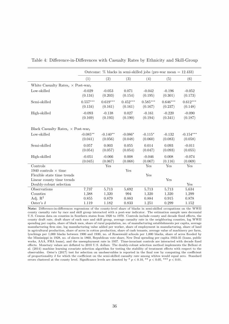
Table 4: Difference-in-Differences with Casualty Rates by Ethnicity and Skill-Group

Outcome: % blacks in semi-skilled jobs (pre-war mean = 12.433)

(1) (2) (3) (4) (5) (6)

White Casualty Ratesc × Post-wart

Low-skilled -0.029 -0.053 0.071 -0.042 -0.196 -0.052(0.134) (0.203) (0.154) (0.195) (0.301) (0.173)

Semi-skilled 0.557∗∗∗ 0.619∗∗∗ 0.452∗∗∗ 0.585∗∗∗ 0.646∗∗∗ 0.612∗∗∗

(0.134) (0.161) (0.161) (0.167) (0.237) (0.148)

High-skilled -0.093 -0.138 0.027 -0.161 -0.220 -0.090(0.169) (0.193) (0.190) (0.194) (0.341) (0.187)

Black Casualty Ratesc × Post-wart

Low-skilled -0.085∗∗ -0.140∗∗ -0.086∗ -0.115∗ -0.132 -0.154∗∗∗

(0.041) (0.056) (0.048) (0.060) (0.083) (0.058)

Semi-skilled 0.057 0.003 0.055 0.014 0.093 -0.011(0.054) (0.057) (0.054) (0.047) (0.093) (0.055)

High-skilled -0.051 -0.066 0.008 -0.046 0.008 -0.074(0.045) (0.067) (0.068) (0.067) (0.116) (0.069)

Controls Yes Yes Yes Yes1940 controls × time YesFlexible state time trends YesLinear county time trends YesDoubly-robust selection YesObservations 7,737 5,713 5,692 5,713 5,713 5,634Counties 1,388 1,320 994 1,320 1,320 1,299Adj. R2 0.855 0.879 0.883 0.884 0.915 0.878Oster’s δ 1.119 1.182 0.833 1.251 0.299 1.152

Note: Difference-in-differences regressions of the county-level share of blacks in semi-skilled occupations on the WWIIcounty casualty rate by race and skill group interacted with a post-war indicator. The estimation sample uses decennialU.S. Census data on counties in Southern states from 1920 to 1970. Controls include county and decade fixed effects, thecounty draft rate, draft share of each race and skill group, average casualty rate in the neighboring counties, log WWIIspending per capita, share of black men, share of rural population, no. of manufacturing establishments per capita, averagemanufacturing firm size, log manufacturing value added per worker, share of employment in manufacturing, share of landin agricultural production, share of acres in cotton production, share of cash tenants, average value of machinery per farm,lynchings per 1,000 blacks between 1900 and 1930, no. of Rosenwald schools per 1,000 blacks, share of acres flooded bythe Mississippi in 1928, no. of slaves in 1860, Republican vote share, New Deal spending per capita 1933-35 (loans, publicworks, AAA, FHA loans), and the unemployment rate in 1937. Time-invariant controls are interacted with decade fixedeffects. Monetary values are deflated to 2010 U.S. dollars. The doubly-robust selection method implements the Belloni etal. (2014) machine learning covariate selection algorithm for testing the stability of treatment effects with respect to theobservables. Oster’s (2017) test for selection on unobservables is reported in the final row by computing the coefficientof proportionality δ for which the coefficient on the semi-skilled casualty rate among whites would equal zero. Standarderrors clustered at the county level. Significance levels are denoted by * p < 0.10, ** p < 0.05, *** p < 0.01.

36

Table 5: Micro Census Triple Differences Results, 1920-1970

Outcome: Pr (semi-skilledizt) = 1

(1) (2) (3) (4) (5) (6)

Panel A: All U.S.

Casualty ratez× Post-wart -0.002 -0.002 -0.002 -0.004 -0.003 -0.009∗∗

(0.007) (0.007) (0.004) (0.004) (0.005) (0.004)

Casualty ratez× Blackizt× 0.047∗∗∗ 0.047∗∗∗ 0.043∗∗∗ 0.019∗∗∗ 0.043∗∗∗ 0.043∗∗∗

Post-wart (0.003) (0.003) (0.003) (0.003) (0.003) (0.003)

Observations 4,348,026 4,348,026 4,335,873 3,119,300 4,335,873 4,335,873Adj. R2 0.031 0.042 0.044 0.135 0.046 0.047

Panel B: South only

Casualty ratez× Post-wart -0.012 -0.013 0.005 -0.009 -0.011 -0.011∗

(0.010) (0.009) (0.007) (0.006) (0.008) (0.006)

Casualty ratez× Blackizt× 0.029∗∗∗ 0.030∗∗∗ 0.028∗∗∗ 0.011∗∗∗ 0.028∗∗∗ 0.028∗∗∗

Post-wart (0.003) (0.003) (0.003) (0.003) (0.003) (0.003)

Observations 1,272,016 1,272,016 1,269,553 911,418 1,269,553 1,269,553Adj. R2 0.061 0.073 0.075 0.140 0.077 0.080

Individual controls Yes Yes Yes Yes YesCommuting Zone controls Yes Yes Yes YesMigration and education YesState time trends YesCommuting zone time trends Yes

Note: Difference-in-differenece-in-differences regression of a semi-skilled indicator on the commuting zone WWII casualtyrate among semi-skilled whites interacted with a post-WWII dummy, and with a black indicator for individuals living in722 commuting zones in the whole U.S. and 300 commuting zones in the South. The estimation sample contains datafrom the decennial U.S. micro Census from 1920-70 on non-institutionalized, working black and white males aged 15-65who are not currently attending school. All regressions include commuting zone and Census year fixed effects. Individuallevel controls include age, marital status, age and place of birth dummies. Column (4) adds cross-state migration andeducation controls interacted with race and time fixed effects. Commuting zone level controls are the WWII draft rate, logWWII spending per capita, share of black men, share of rural population, no. of manufacturing establishments per capita,average manufacturing firm size, log manufacturing value added per worker, share of employment in manufacturing, shareof land in agricultural production, share of acres in cotton production, share of cash tenants, average value of machineryper farm, lynchings per 1,000 blacks between 1900 and 1930, no. of Rosenwald schools per 1,000 blacks, share of acresflooded by the Mississippi in 1928, no. of slaves in 1860, Republican vote share, New Deal spending per capita 1933-35(loans, public works, AAA, FHA loans), and the unemployment rate in 1937. Time-invariant controls are interacted withdecade fixed effects. Monetary values are deflated to 2010 U.S. dollars. Standard errors clustered at the commuting zonelevel in parentheses. Significance levels are denoted by * p < 0.10, ** p < 0.05, *** p < 0.01.

37

Table 6: Triple Differences Results by Industry, 1920-1970

Outcome: Pr (semi-skilledizt) = 1

Manufacturing

All Durable Non-Durable(1) (2) (3)

Casualty ratez× Post-wart -0.004 -0.006 0.016(0.007) (0.006) (0.012)

Casualty ratez× Blackizt× Post-wart 0.097∗∗∗ 0.086∗∗∗ 0.105∗∗∗

(0.005) (0.004) (0.006)Observations 1,378,824 519,224 860,182Adj. R2 0.038 0.040 0.042

Comparison Sectors

Telecom. Retail Public Admin.(1) (2) (3)

Casualty ratez× Post-wart -0.003 0.000 0.002(0.014) (0.004) (0.011)

Casualty ratez× Blackizt× Post-wart 0.024 -0.008∗∗∗ 0.001(0.016) (0.003) (0.006)

Observations 39,510 469,259 361,325Adj. R2 0.095 0.027 0.359

Note: Difference-in-differenece-in-differences regression of a semi-skilled indicator on the commuting zone WWII casualtyrate among semi-skilled whites interacted with a post-WWII dummy, and with a black indicator. The estimation samplecontains data from the decennial U.S. micro Census from 1920-70 on non-institutionalized, working black and white malesaged 15-65. Regression results for semi-skill (columns 1-3) and high-skill (columns 4-6) intensive sectors. All regressionsinclude commuting zone and Census year fixed effects. Individual level controls include age, marital status, age and placeof birth dummies. Commuting zone level controls are the WWII draft rate, log WWII spending per capita, share ofblack men, share of rural population, no. of manufacturing establishments per capita, average manufacturing firm size, logmanufacturing value added per worker, share of employment in manufacturing, share of land in agricultural production,share of acres in cotton production, share of cash tenants, average value of machinery per farm, lynchings per 1,000 blacksbetween 1900 and 1930, no. of Rosenwald schools per 1,000 blacks, share of acres flooded by the Mississippi in 1928, no.of slaves in 1860, Republican vote share, New Deal spending per capita 1933-35 (loans, public works, AAA, FHA loans),and the unemployment rate in 1937. Time-invariant controls are interacted with decade fixed effects. Monetary values aredeflated to 2010 U.S. dollars. Standard errors clustered at the commuting zone level in parentheses. Significance levels aredenoted by * p < 0.10, ** p < 0.05, *** p < 0.01.

38

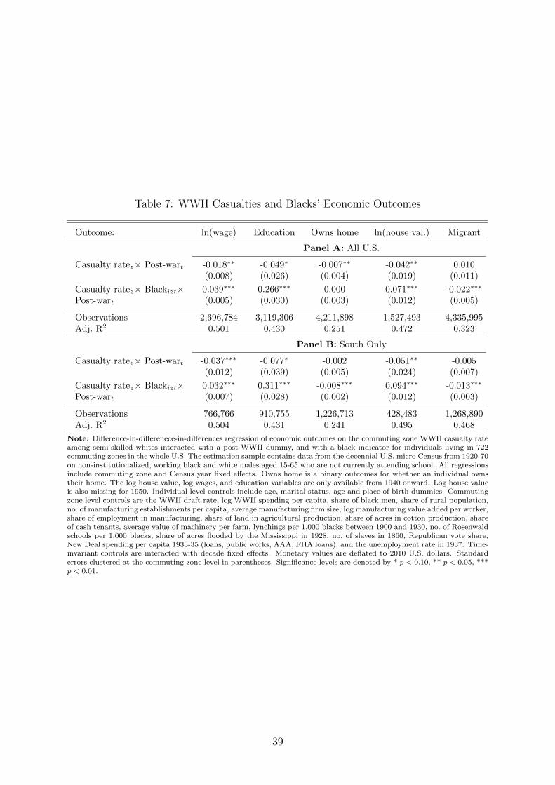
Table 7: WWII Casualties and Blacks’ Economic Outcomes

Outcome: ln(wage) Education Owns home ln(house val.) Migrant

Panel A: All U.S.

Casualty ratez× Post-wart -0.018∗∗ -0.049∗ -0.007∗∗ -0.042∗∗ 0.010(0.008) (0.026) (0.004) (0.019) (0.011)

Casualty ratez× Blackizt× 0.039∗∗∗ 0.266∗∗∗ 0.000 0.071∗∗∗ -0.022∗∗∗

Post-wart (0.005) (0.030) (0.003) (0.012) (0.005)

Observations 2,696,784 3,119,306 4,211,898 1,527,493 4,335,995Adj. R2 0.501 0.430 0.251 0.472 0.323

Panel B: South Only

Casualty ratez× Post-wart -0.037∗∗∗ -0.077∗ -0.002 -0.051∗∗ -0.005(0.012) (0.039) (0.005) (0.024) (0.007)

Casualty ratez× Blackizt× 0.032∗∗∗ 0.311∗∗∗ -0.008∗∗∗ 0.094∗∗∗ -0.013∗∗∗

Post-wart (0.007) (0.028) (0.002) (0.012) (0.003)

Observations 766,766 910,755 1,226,713 428,483 1,268,890Adj. R2 0.504 0.431 0.241 0.495 0.468

Note: Difference-in-differenece-in-differences regression of economic outcomes on the commuting zone WWII casualty rateamong semi-skilled whites interacted with a post-WWII dummy, and with a black indicator for individuals living in 722commuting zones in the whole U.S. The estimation sample contains data from the decennial U.S. micro Census from 1920-70on non-institutionalized, working black and white males aged 15-65 who are not currently attending school. All regressionsinclude commuting zone and Census year fixed effects. Owns home is a binary outcomes for whether an individual ownstheir home. The log house value, log wages, and education variables are only available from 1940 onward. Log house valueis also missing for 1950. Individual level controls include age, marital status, age and place of birth dummies. Commutingzone level controls are the WWII draft rate, log WWII spending per capita, share of black men, share of rural population,no. of manufacturing establishments per capita, average manufacturing firm size, log manufacturing value added per worker,share of employment in manufacturing, share of land in agricultural production, share of acres in cotton production, shareof cash tenants, average value of machinery per farm, lynchings per 1,000 blacks between 1900 and 1930, no. of Rosenwaldschools per 1,000 blacks, share of acres flooded by the Mississippi in 1928, no. of slaves in 1860, Republican vote share,New Deal spending per capita 1933-35 (loans, public works, AAA, FHA loans), and the unemployment rate in 1937. Time-invariant controls are interacted with decade fixed effects. Monetary values are deflated to 2010 U.S. dollars. Standarderrors clustered at the commuting zone level in parentheses. Significance levels are denoted by * p < 0.10, ** p < 0.05, ***p < 0.01.

39

Table 8: Interview Questions and Outcome Coding Scheme

I Interracial Friend: (Var 0377)“Have you ever known a white (colored) person well enough that you would talk to him as afriend?”Coded 1 for 1 (Yes), and 0 otherwise.

I Live in Mixed Area: (Var 0079)“Racial composition of residential area of respondent”Coded 1 for value 3 (Mixed).

I Favor Integration: (Var 0374) “Are you in favor of integration, strict segregation, or somethingin between?”Coded 1 for 2 (Integration), and 0 otherwise.

I Favor Mixed Churches: (Var 0397)“Inter-racial contact: churches - Respondent favors:”Coded 1 for values 4 (Gradual integration), 5 (Rapid integration) and 6 (Mixed), and 0 otherwise.

I Favor Mixed Schools: (Var 0396)“Inter-racial contact: schools - Respondent favors:”Coded 1 for values 4 (Gradual integration), 5 (Rapid integration) and 6 (Mixed), and 0 otherwise.

I Priest Pro Segregation: (Var 0164)“Would you say that your minister believes that religion or the Bible favors segregation or inte-gration?”Coded 1 for 1 (Favors segregation) and 2 (Qualified favors segregation), and 0 otherwise.

Note: Original questions from the 1961 “Negro Political Participation Study” (Matthews and Prothro, 1975) and thedefinitions of the outcome variables which are coded from the corresponding questions as binary variables. Outcomes arein bold font, questionnaire variable numbers are reported in parentheses, questions from the survey between in quotationmarks, followed by the coding scheme for the binary variables. The code book for ICPSR study number 7255 is freelyavailable at: http://www.icpsr.umich.edu/icpsrweb/ICPSR/studies/7255

Table 9: Summary Statistics - Outcome Variables by Race

Black (n = 540) White (n = 528) Difference

mean st. dev. mean st. dev. diff. s.e.Interracial Friend 0.466 0.499 0.583 0.494 0.117*** 0.030Live in Mixed Area 0.161 0.368 0.085 0.279 -0.076*** 0.020Favor Integration 0.641 0.480 0.036 0.186 -0.605*** 0.022Favor Mixed Churches 0.057 0.233 0.011 0.106 -0.046*** 0.011Favor Mixed Schools 0.059 0.236 0.045 0.208 -0.014 0.014Priest Pro Segregation 0.061 0.240 0.142 0.349 0.081*** 0.018

Note: Binary outcomes of the social and political integration, standing and attitudes of blacks for black and whiterespondents in the “Negro Political Participation Study” of 1961 (Matthews and Prothro, 1975). Only individuals inthe final estimation sample were used to produce these summary statistics. Differences in means and the correspondingstandard errors were estimated with t-tests. Significance levels at 10%, 5%, and 1% are denoted by *, **, ***, respectively.The question about repercussions for political activity against blacks were only asked to African American respondents.

40

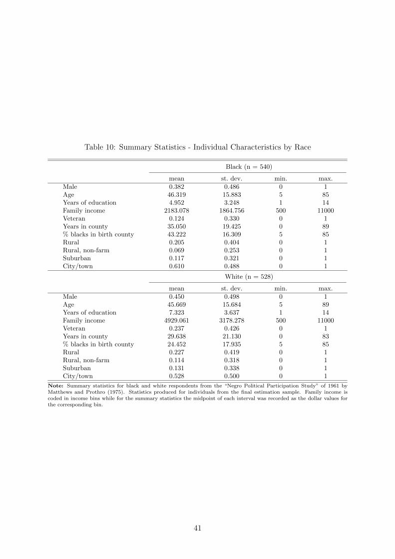
Table 10: Summary Statistics - Individual Characteristics by Race

Black (n = 540)

mean st. dev. min. max.Male 0.382 0.486 0 1Age 46.319 15.883 5 85Years of education 4.952 3.248 1 14Family income 2183.078 1864.756 500 11000Veteran 0.124 0.330 0 1Years in county 35.050 19.425 0 89% blacks in birth county 43.222 16.309 5 85Rural 0.205 0.404 0 1Rural, non-farm 0.069 0.253 0 1Suburban 0.117 0.321 0 1City/town 0.610 0.488 0 1

White (n = 528)

mean st. dev. min. max.Male 0.450 0.498 0 1Age 45.669 15.684 5 89Years of education 7.323 3.637 1 14Family income 4929.061 3178.278 500 11000Veteran 0.237 0.426 0 1Years in county 29.638 21.130 0 83% blacks in birth county 24.452 17.935 5 85Rural 0.227 0.419 0 1Rural, non-farm 0.114 0.318 0 1Suburban 0.131 0.338 0 1City/town 0.528 0.500 0 1

Note: Summary statistics for black and white respondents from the “Negro Political Participation Study” of 1961 byMatthews and Prothro (1975). Statistics produced for individuals from the final estimation sample. Family income iscoded in income bins while for the summary statistics the midpoint of each interval was recorded as the dollar values forthe corresponding bin.

41

Table 11: The Skill Upgrade and Black-White Social Relations - OLS and IV Results

Pr(Interracial Friend)=1 Pr(Live in Mixed Race Area)=1

(OLS) (IV) (OLS) (IV)

∆semi-skilled blacksc 0.0181 0.0180 0.0155 0.0118(0.0059)∗∗∗ (0.0075)∗∗ (0.0046)∗∗∗ (0.0046)∗∗∗

[0.0079]∗∗ [0.0103]∗ [0.0062]∗∗ [0.0075]

Outcome mean 0.5235 0.5235 0.1236 0.1236R2 0.1213 0.1213 0.1406 0.1402

Pr(Favor Integration)=1 Pr(Favor Mixed Schools)=1

(OLS) (IV) (OLS) (IV)

∆semi-skilled blacksc 0.0097 0.0211 0.0105 0.0104(0.0031)∗∗∗ (0.0062)∗∗∗ (0.0021)∗∗∗ (0.0032)∗∗∗

[0.0053]∗ [0.0123]∗ [0.0039]∗∗∗ [0.0047]∗∗

Outcome mean 0.3418 0.3418 0.0524 0.0524R2 0.5097 0.5079 0.0683 0.0683

Pr(Favor Mixed Church)=1 Pr(Priest Pro Segregation)=1

(OLS) (IV) (OLS) (IV)

∆semi-skilled blacksc 0.0027 0.0075 −0.0051 −0.0146(0.0015)∗ (0.0021)∗∗∗ (0.0039) (0.0069)∗∗

[0.0021] [0.0033]∗∗ [0.0052] [0.0104]

Outcome mean 0.0346 0.0346 0.1011 0.1011R2 0.0801 0.0780 0.1191 0.1160

Note: The estimation sample is kept constant in all regressions with 540 black and 528 white adults in 24 counties fromSouthern states in 1961 using data from the “Negro Political Participation Study” (Matthews and Prothro, 1975). Thechange in the share of blacks in semi-skilled employment from 1940 to 1950 (∆share of blacksc) in county c is instrumentedwith the WWII casualty rate among semi-skilled whites in that county. The first stage F-statistic is 43.799 and the Oleaand Pflueger (2013) efficient F-statistic is 45.841. Individual level controls include gender, race, age, location of dwelling(urban, suburban, rural), years lived in current county, place size, veteran status, county where a respondent grew up, andstate fixed effects. County level controls used are the share of blacks in semi-skilled jobs in 1940, the share of blacks incounty c, share of people not born in county c, the WWII draft rate, and variables on racial sentiment such as the numberof Rosenwald schools per 1,000 blacks, the number of lynchings from 1900-30 per 1,000 blacks, and the number of blackslaves in 1860. Standard errors are clustered at the county level and are reported in parentheses. Standard errors correctedfor the small cluster size using the wild cluster bootstrap-t procedure for OLS models by Cameron et al. (2008) and the wildrestricted efficient residual bootstrap for IV models by Davidson and MacKinnon (2010) are reported in squared brackets.Significance levels are denoted by ∗ p < 0.10, ∗∗ p < 0.05, ∗∗∗ p < 0.01.

42

Figures

Figure 1: Share of Semi- and High-Skilled Employment Among Black Men, 1870 to 2010

(a) All U.S.

WWII

010

2030

4050

%

1870 1880 1900 1910 1920 1930 1940 1950 1960 1970 1980 1990 2000 2010

semi-skilled high-skilled

1

(b) Southern U.S.

WWII

010

2030

4050

%

1870 1880 1900 1910 1920 1930 1940 1950 1960 1970 1980 1990 2000 2010

semi-skilled high-skilled

1

Note: Graphs are based on the public use microdata files of the 1870-2010 Decennial U.S. Censusesby Ruggles et al. (2018). The sample includes black males aged 16 to 65 of the non-institutionalizedpopulation who are not attending school at the enumeration date. Semi-skilled jobs (dots) areoperatives and craftsmen, and high-skilled jobs (diamonds) are clerks, professionals, and managers.Occupations are defined according to the 1950 Census Bureau occupational classification scheme.The years of U.S. involvement in World War II are marked with light gray background shading.Data for the South includes individuals living in the states of the former Confederacy, as well asDelaware, DC, Kentucky, Maryland, Oklahoma, and West Virginia.

43

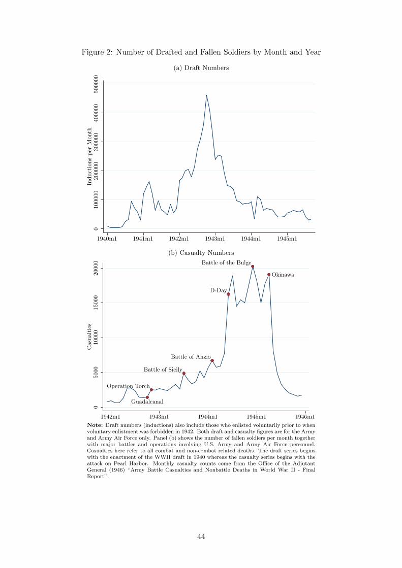
Figure 2: Number of Drafted and Fallen Soldiers by Month and Year

(a) Draft Numbers

0100000

200000

300000

400000

500000

Inductionsper

Mon

th

1940m1 1941m1 1942m1 1943m1 1944m1 1945m1

1

(b) Casualty Numbers

Guadalcanal

Operation Torch

Battle of Sicily

Battle of Anzio

D-Day

Battle of the Bulge

Okinawa

05000

10000

15000

20000

Casualties

1942m1 1943m1 1944m1 1945m1 1946m1

1

Note: Draft numbers (inductions) also include those who enlisted voluntarily prior to whenvoluntary enlistment was forbidden in 1942. Both draft and casualty figures are for the Armyand Army Air Force only. Panel (b) shows the number of fallen soldiers per month togetherwith major battles and operations involving U.S. Army and Army Air Force personnel.Casualties here refer to all combat and non-combat related deaths. The draft series beginswith the enactment of the WWII draft in 1940 whereas the casualty series begins with theattack on Pearl Harbor. Monthly casualty counts come from the Office of the AdjutantGeneral (1946) “Army Battle Casualties and Nonbattle Deaths in World War II - FinalReport”.

44

Figure 3: Draft and Casualty Records Example

(a) IBM Draft Punch Card

(b) WWII Honor List of Dead and Missing

Note: Panel a) shows the enlistment punch card for James Tronolone from Erie, New York, born in 1910. His Army serialnumber is shown on the top left corner of the card, his rank, date of enlistment, and service branch, among other, onthe top right. Panel b) shows an excerpt from the WWII Honor List of Dead and Missing for Warwick County, Virginia.The table displays a soldier’s name, their Army serial number, rank, and cause of death. Source: National Archives andRecords Administration, Record Group 407: Records of the Adjutant General’s Office, 1917- [AGO].

45

Figure 4: WWII Casualty Rates among Semi-Skilled Whites in the U.S. South

4.10 - 22.22%

3.16 - 4.10%

2.38 - 3.16%

1.16 - 2.38%

0.00 - 1.16%

Casualty rate

1

Note: Spatial distribution of WWII casualty rates among semi-skilled white men at the county level in percent. Shadedpolygons display the quintiles of the casualty rate distribution with ranges being shown in the legend on the side. Southernstates included here are Alabama, Arkansas, Delaware, Florida, Georgia, Kentucky, Louisiana, Maryland, Mississippi,North Carolina, South Carolina, Oklahoma, Tennessee, Texas, Virginia, and West Virginia.

46

Figure 5: Scatter Plots for WWII Casualty Rates and the Share of Blacks in Semi-SkilledJobs in Levels and First Differences

(a) Correlation with the Semi-Skilled Share Level in 1950

β = 1.854(0.175)

1520

2530

Shareof

Blacksin

Sem

i-SkilledJob

s

0 2 4 6 8 10

10

WWII Casualty Rate (Semi-Skilled Whites)

1

(b) Correlation with the Semi-Skilled Share 1940 to 50 First Difference

β = 0.623(0.072)

∆Shareof

Blacksin

Sem

i-SkilledJob

s1940-50

0

0

2

2

4

4

6

6

8

8

10WWII Casualty Rate (Semi-Skilled Whites)

1

Note: Scatter plots of the relation between the WWII casualty rate among semi-skilledwhites and the share of blacks in semi-skilled employment in 1950 across counties (panel a),and the change in the share of blacks in semi-skilled employment from 1940 to 1950 (panelb).

47

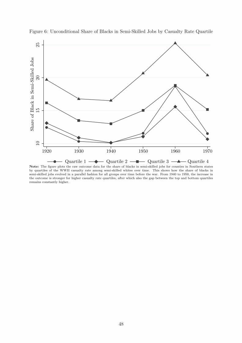
Figure 6: Unconditional Share of Blacks in Semi-Skilled Jobs by Casualty Rate Quartile10

1520

25Shareof

Black

inSem

i-SkilledJob

s

1920 1930 1940 1950 1960 1970

Quartile 1 Quartile 2 Quartile 3 Quartile 4

1

Note: The figure plots the raw outcome data for the share of blacks in semi-skilled jobs for counties in Southern statesby quartiles of the WWII casualty rate among semi-skilled whites over time. This shows how the share of blacks insemi-skilled jobs evolved in a parallel fashion for all groups over time before the war. From 1940 to 1950, the increase inthe outcome is stronger for higher casualty rate quartiles, after which also the gap between the top and bottom quartilesremains constantly higher.

48

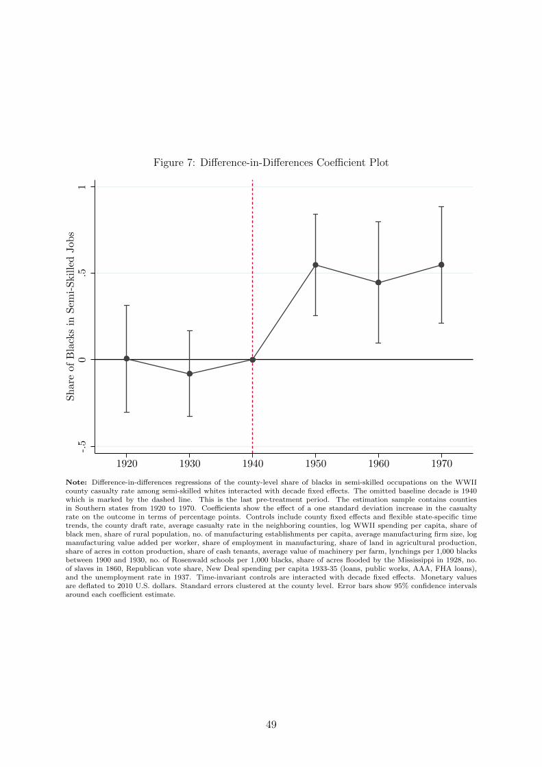
Figure 7: Difference-in-Differences Coefficient Plot

PSfrag replacements

-.5

0.5

1Shareof

Blacksin

Sem

i-SkilledJob

s

1920 1930 1940 1950 1960 1970

1

Note: Difference-in-differences regressions of the county-level share of blacks in semi-skilled occupations on the WWIIcounty casualty rate among semi-skilled whites interacted with decade fixed effects. The omitted baseline decade is 1940which is marked by the dashed line. This is the last pre-treatment period. The estimation sample contains countiesin Southern states from 1920 to 1970. Coefficients show the effect of a one standard deviation increase in the casualtyrate on the outcome in terms of percentage points. Controls include county fixed effects and flexible state-specific timetrends, the county draft rate, average casualty rate in the neighboring counties, log WWII spending per capita, share ofblack men, share of rural population, no. of manufacturing establishments per capita, average manufacturing firm size, logmanufacturing value added per worker, share of employment in manufacturing, share of land in agricultural production,share of acres in cotton production, share of cash tenants, average value of machinery per farm, lynchings per 1,000 blacksbetween 1900 and 1930, no. of Rosenwald schools per 1,000 blacks, share of acres flooded by the Mississippi in 1928, no.of slaves in 1860, Republican vote share, New Deal spending per capita 1933-35 (loans, public works, AAA, FHA loans),and the unemployment rate in 1937. Time-invariant controls are interacted with decade fixed effects. Monetary valuesare deflated to 2010 U.S. dollars. Standard errors clustered at the county level. Error bars show 95% confidence intervalsaround each coefficient estimate.

49

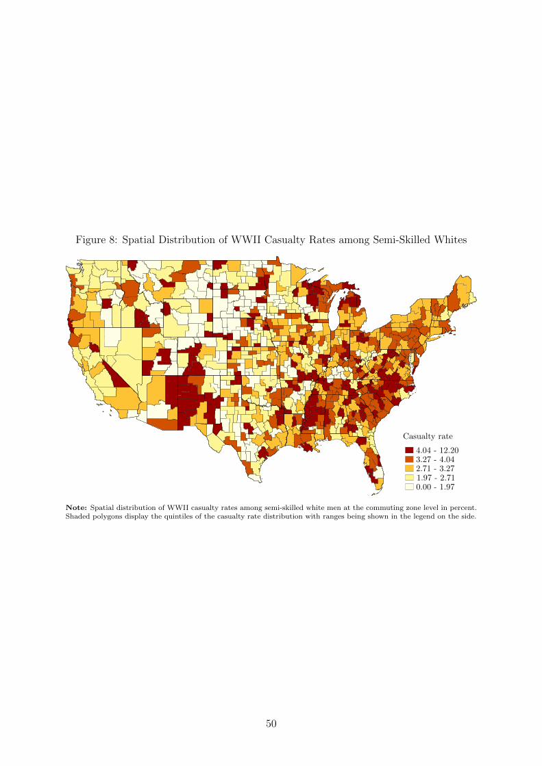
Figure 8: Spatial Distribution of WWII Casualty Rates among Semi-Skilled Whites

4.04 - 12.203.27 - 4.042.71 - 3.271.97 - 2.710.00 - 1.97

Casualty rate

1

Note: Spatial distribution of WWII casualty rates among semi-skilled white men at the commuting zone level in percent.Shaded polygons display the quintiles of the casualty rate distribution with ranges being shown in the legend on the side.

50

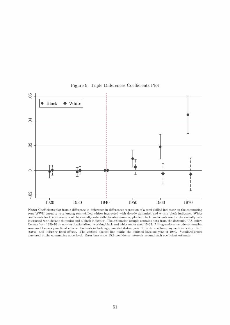
Figure 9: Triple Differences Coefficients Plot

-.02

0.02

.04

.06

1920 1930 1940 1950 1960 1970

Black White

1

Note: Coefficients plot from a difference-in-difference-in-differences regression of a semi-skilled indicator on the commutingzone WWII casualty rate among semi-skilled whites interacted with decade dummies, and with a black indicator. Whitecoefficients for the interaction of the casualty rate with decade dummies, plotted black coefficients are for the casualty rateinteracted with decade dummies and a black indicator. The estimation sample contains data from the decennial U.S. microCensus from 1920-70 on non-institutionalized, working black and white males aged 15-65. All regressions include commutingzone and Census year fixed effects. Controls include age, marital status, year of birth, a self-employment indicator, farmstatus, and industry fixed effects. The vertical dashed line marks the omitted baseline year of 1940. Standard errorsclustered at the commuting zone level. Error bars show 95% confidence intervals around each coefficient estimate.

51

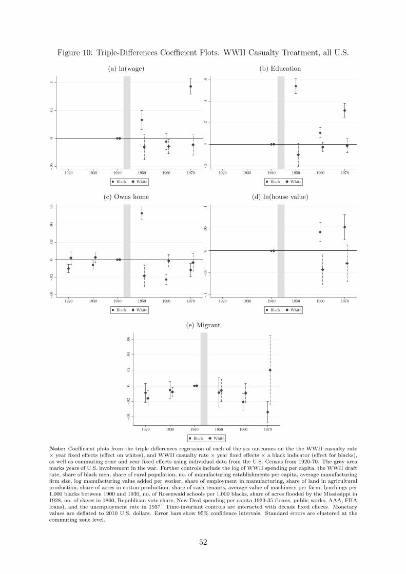
Figure 10: Triple-Differences Coefficient Plots: WWII Casualty Treatment, all U.S.

(a) ln(wage)

-.05

0.05

.1

1920 1930 1940 1950 1960 1970

Black White

1

(b) Education

-.2

0.2

.4.6

1920 1930 1940 1950 1960 1970

Black White

1

(c) Owns home

-.04

-.02

0.02

.04

.06

1920 1930 1940 1950 1960 1970

Black White

1

(d) ln(house value)-.1

-.05

0.05

.1

1920 1930 1940 1950 1960 1970

Black White

1

(e) Migrant

-.04

-.02

0.02

.04

.06

1920 1930 1940 1950 1960 1970

Black White

1

Note: Coefficient plots from the triple differences regression of each of the six outcomes on the the WWII casualty rate× year fixed effects (effect on whites), and WWII casualty rate × year fixed effects × a black indicator (effect for blacks),as well as commuting zone and year fixed effects using individual data from the U.S. Census from 1920-70. The gray areamarks years of U.S. involvement in the war. Further controls include the log of WWII spending per capita, the WWII draftrate, share of black men, share of rural population, no. of manufacturing establishments per capita, average manufacturingfirm size, log manufacturing value added per worker, share of employment in manufacturing, share of land in agriculturalproduction, share of acres in cotton production, share of cash tenants, average value of machinery per farm, lynchings per1,000 blacks between 1900 and 1930, no. of Rosenwald schools per 1,000 blacks, share of acres flooded by the Mississippi in1928, no. of slaves in 1860, Republican vote share, New Deal spending per capita 1933-35 (loans, public works, AAA, FHAloans), and the unemployment rate in 1937. Time-invariant controls are interacted with decade fixed effects. Monetaryvalues are deflated to 2010 U.S. dollars. Error bars show 95% confidence intervals. Standard errors are clustered at thecommuting zone level.

52

Figure 11: Triple-Differences Coefficient Plots: WWII Casualty Treatment, South only

(a) ln(wage)

-.05

0.05

.1.15

1920 1930 1940 1950 1960 1970

Black White

1

(b) Education

-.2

0.2

.4.6

1920 1930 1940 1950 1960 1970

Black White

1

(c) Owns home

-.04

-.02

0.02

.04

1920 1930 1940 1950 1960 1970

Black White

1

(d) ln(house value)-.1

-.05

0.05

.1

1920 1930 1940 1950 1960 1970

Black White

1

(e) Migrant

-.03

-.02

-.01

0.01

1920 1930 1940 1950 1960 1970

Black White

1

Note: Coefficient plots from the triple differences regression of each of the six outcomes on the the WWII casualty rate× year fixed effects (effect on whites), and WWII casualty rate × year fixed effects × a black indicator (effect for blacks),as well as commuting zone and year fixed effects using individual data from the U.S. Census from 1920-70. The gray areamarks years of U.S. involvement in the war. The sample includes observations from Southern states only. Further controlsinclude the log of WWII spending per capita, the WWII draft rate, share of black men, share of rural population, no. ofmanufacturing establishments per capita, average manufacturing firm size, log manufacturing value added per worker, shareof employment in manufacturing, share of land in agricultural production, share of acres in cotton production, share of cashtenants, average value of machinery per farm, lynchings per 1,000 blacks between 1900 and 1930, no. of Rosenwald schoolsper 1,000 blacks, share of acres flooded by the Mississippi in 1928, no. of slaves in 1860, Republican vote share, New Dealspending per capita 1933-35 (loans, public works, AAA, FHA loans), and the unemployment rate in 1937. Time-invariantcontrols are interacted with decade fixed effects. Monetary values are deflated to 2010 U.S. dollars. Error bars show 95%confidence intervals. Standard errors are clustered at the commuting zone level.

53

Figure 12: Location of NPPS Respondents

Note: Counties included in the “Negro Political Participation Study” by Matthews in Prothro (1975) in 1961. Some stateswhich were chosen for the main analysis are not included in this sample. Matthews and Prothro (1975) only included thosestates and counties which officially belonged to the former Confederacy. Hence border states such as Kentucky, Maryland,Delaware and West Virginia are not included. Oklahoma was Indian Territory at the time and therefore also was notincluded in the list of Confederate states belonging to the NPPS sampling scheme.

54

Appendices

A Black occupational upgrade

A1) Robustness and Heterogeneity

A1.1: Parallel Trends Assumptions

In addition to the lags and leads of the casualty treatment and their effects on the share

of blacks in semi-skilled jobs in figure 7, figure 13 provides the same plot under different

model specifications. This includes the model without covariates (i.e. the raw data less

time and county fixed effects), with controls, with controls fixed at their 1940 values

and interacted with time dummies, and controls selected by the Belloni et al. (2014)

algorithm. The insignificance of the pre-trends and the post-war treatment effect do not

hinge on any particular model specification but are indistinguishable from the coefficients

plot presented in the main section.

A1.2: Selection on Observables

Table 12 estimates the DiD model in eq. (2) and gradually expands the covariate set.

Observing the movement of the coefficient of interest shows that the casualty rate coeffi-

cient stabilizes at around 0.59 p.p. There is no one particular control which significantly

alters the results after being included. The typical argument is that the treatment effect

remains stable with respect to the inclusion of observed factors, it would remain stable

also with respect to unobserved factors. However, as discussed in the main section with

reference to Oster’s (2017) test, this is not necessarily true if, for instance, observables and

unobservables are unrelated to each other but separately affect the relationship between

treatment and outcome.

A downside of the coefficient stability test is that invariance of the top-row coefficient

might be due to measurement error in the controls. Following Pei et al. (2018), a more

powerful alternative is to take the added control to the left-hand side of the equation and

test for imbalances with respect to the treatment variable. This is equivalent to running

regressions with and without the added control and comparing both estimates via a SUR

regression. This is a generalized Hausman test. The corresponding χ2 test statistics and

p-values are reported in the bottom two rows of table 12. The test reveals no significant

imbalances in the controls which are related to the casualty rate.

55

A1.3: Selective Migration of Blacks

Even though the casualty rate need not be random in this estimation framework, a

potential threat to identification are time-varying confounding factors or systematic ma-

nipulation of individuals’ treatment status. With the war period being a major episode

of migration for blacks from the South (Boustan, 2016), a plausible issue could arise if

blacks migrated from low- to high-casualty counties to find semi-skilled employment. In

this case, the casualty rate effect picks up an additional migratory response.

To test for this possibility, I re-estimate eq. (3) using the share of blacks and the

share of black men in a given county as dependent variable. The results for this cross-

county migration test are shown in figure 14. None of the estimated coefficients are

significant, neither statistically nor economically. This finding is consistent with the

previous balancing test by Pei et al. (2018) in table 12 for the share of black men. The

result also suggests that if blacks gained semi-skilled employment due to the war-induced

lack of white workers in this skill-group, then they must have done so in their current

counties of residence.

Even if the 1950 interaction in figure 14 was significantly different from zero, it would

imply that the share of blacks in a given county increased by 0.05 p.p. for a one percentage

point increase in the casualty rate. Relative to a pre-war average of 22.36%, such an

increase would not be considered an economically significant migratory response. The

result for the share of black men is the same. This is not to say that African Americans

were not migrating during this period. They just did not do so differentially across high-

and low-casualty rate counties. Appendix B uses data from the micro Census to provide

further evidence that the findings here are not driven by migration patterns by black

workers.

A1.4: Selection of Soldiers

Table 13 reports DiD results of eq. (2) including average soldier characteristics by county

interacted with a post-war indicator. These characteristics include the average age, years

of education, AGCT score (an aptitude test which is the predecessor of the AFQT), share

of married, and share of voluntarily enlisted soldiers. This is to preclude the possibility

that soldiers from particularly patriotic counties volunteer and die, but that these are

also the types of counties where people become more attached to each other and less

prejudiced on racial grounds in times of hardship.

56

The results are unchanged by including these variables. In addition, figure 17 shows

that there are no marked differences in voluntary enlistments between a) the South and

the rest of the country and b) above and below median casualty rate counties within

the South. While soldiers are certainly selected (e.g. illiterates were service ineligible),

the selection into the military and into death does not appear to affect the relationship

between the WWII casualty rates among semi-skilled whites and the share of blacks in

this skill group.

A1.5: Alternative Treatment Denominators and Denominator Bias

In this section I consider an alternative definition of the treatment variable as compared

to eq. (1) which used the number of semi-skilled white soldiers as denominator. The

rational was to account for unobservable draft deferments. Results using as denominator

all semi-skilled white workers,

Casualty ratec =Number of fallen semi-skilled white soldiersc

Number of semi-skilled white workersc× 100 (8)

are reported in table 14. This casualty variable has a mean of 0.55, standard deviation

of 1.39, minimum of zero, and maximum of 25.54. In all specifications the casualty rate

effect is positive and significant at the one percent level. Compared to the baseline specifi-

cation the coefficients are larger and slightly more volatile with respect to their magnitude

when county-specific linear time trends are included. The corresponding coefficients plot

for the lags and leads of this treatment variable is shown in figure 16.

Another concern is that there might be a spurious relationship between the share of

blacks in semi-skilled occupations the the casualty rate among semi-skilled whites due

to a correlation between the denominators which is driving the estimated change. To

account for this, I fix the outcome denominator in eq. (1) at it’s pre-war level in 1940.

This will result in shares that are not necessarily bound in the [0, 1] interval but are

indicative for whether results are sensitive with respect to changes in the denominator.

Table 15 reports the estimation results. All but the last column show a positive effect

which is significant at the five percent level or less.

A1.6: Sensitivity of Results by State

To test whether results are driven by any given state, I re-estimate the DiD specification in

eq. 2 using the sample with counties from the S−1 states. The results from this jackknife-

57

type leave-one-out procedure are shown in figure 18. The figure plots the estimated WWII

casualty rate DiD coefficient for each iteration with the left-out state in a given regression

being displayed on the vertical axis. The resulting coefficients are indistinguishable from

each other as well as from the main result in table 3.

A1.6: Spatial Clustering of Casualty Rates

U.S. military units were raised locally during WWII, a practice that was abandoned after

D-Day. This policy as well as the patterns observed in the map in figure 4 may hint

towards spatial dependencies in the outcome. Such spatial correlation would pose prob-

lems for inference whereby standard errors are underestimated. To test for such spatial

autocorrelation, I compute Moran’s (1950) I statistic for global spatial correlation and

the Getis-Ord G∗i (d) statistic (Getis and Ord, 1992) to test for local spatial correlation.

Moran’s I is computed as

I =

∑ni=1

∑nj=1wijCiCj∑ni=1C

2i

(9)

where i indexes counties with a total number of n counties, j indexes all other counties

with i 6= j, C is the WWII casualty rate among semi-skilled whites, and w is a spatial

weight matrix. Like the standard correlation coefficient, Moran’s I lies in [−1, 1]. The z

score for the corresponding test statistic is given by:

z(I) =I − E(I)√V ar(I)

Results from this test are reported in table 17 for distance thresholds of 200, 400, and

600km. Columns (1) to (3) show the casualty rate has a small but statistically significant

positive spatial autocorrelation at the 1% level across counties. Moran’s I ranges between

0.049 and 0.078. However, once the casualty rate is demeaned by its state-specific aver-

ages, Moran’s I drops to between -0.003 and -0.008 and becomes insignificant except for

the 400km distance threshold where it is marginally significant at the 10% level. This

implies that once state fixed effects are controlled for, the casualty rate measure is as good

as randomly assigned across geographic space. In the main DiD specifications, these fixed

effects would be absorbed by the county fixed effects.

Spatial correlation, however, may exist at a more concentrated level. To test for more

58

local correlations, I provide estimates of the Getis-Ord G∗i (d) statistic:

G∗i (d) =

∑nj=1wij(d)Cj∑n

i=1Cj(10)

where the notation is as before except that now the spatial weight matrix depends on

a certain radius d within which the statistic is computed.18 Clusters of counties with

significantly higher casualty rates are referred to as hot spots. Conversely, those with

significantly lower casualty rates are called cold spots.

Table 18 reports the results from the Getis-Ord test for the same 200, 400, and 600km

distance bands as before. The table reports the number of counties within a given z-score

interval. Casualty rates show local spatial independence if the z-score of G∗i (d) falls within

-1.96 and 1.96. Lower z-scores than the lower bound of -1.96 indicate cold spots while

higher values than 1.96 indicate hot spots. Again, columns (1) to (3) indicate local spatial

correlation with a significant number of counties displaying cold spots (365 counties) and

409 counties having hot spots, out of a total of 1,387 counties. Once state fixed effects

are partialled out, almost all counties lose this local spatial autocorrelation as is shown

in columns (4) to (6).

Even though spatial correlation appears to be accounted for by geographic fixed ef-

fects, I replicate the main findings in table 3 and compute Conley (1999) standard errors

to correct for spatial dependence.19 Table 19 reports the results and shows that the

significance of previous results is not driven by spatial autocorrelation.

A1.7: Alternative Regression Specification

Studying the relationship between war casualties and semi-skilled employment for blacks

in shares relates directly to the opening graph in figure 1. An alternative way of looking

at this relation is to run the regression in eq. 2 using the levels and taking first differences:

∆blacks in semi-skilled jobsct = βwhite semi-skilled casualtiesc × post-wart

+ γt +X ′ctξ + ηct (11)

18For both Moran’s I and the Getis-Ord G∗i (d) binary spatial weights matrices were used. Changing

these to exponential or power function type spatial weight matrices does not alter the results. Additionalresults with alternative spatial weight matrices are not reported here but are available on request. TheStata routine getisord by Kondo (2016) was used to compute this test.

19Thiemo Fetzer’s reg2hdfespatial Stata routine was used to run these regressions.

59

I control for the total county population and the number of drafted men in addition to

the other controls which are the same as in section 3. The results from estimating eq.

(11) are reported in table 16. On average, a fallen white semi-skilled worker is replaced

by four to six African Americans. This is a consistent result across all specifications

and shows up with significant coefficients. The exception is column (5) which includes

county-specific linear time trends.

The next question is then why there is not a one-to-one substitution between white

and black workers. There are several potential explanations. A pessimistic view would

be that blacks are less productive and hence it requires more workers from this group to

substitute a white worker. Boustan (2009) finds that blacks who migrate North are not

perfect substitutes for white workers. She estimates an elasticity of substitution between

black and white males of similar skill of 8.3 to 11.1. However, this is likely not only driven

by characteristics of African American workers but also by institutional factors such as

wage discrimination. Her estimated elasticities are lower than those from the literature

on the substitutability between natives and foreigners. This literature finds elasticities

in the range of 20 to 47 (see Pari and Sparber, 2009).20

A more optimistic view is provided by a learning-by-doing argument on part of the

employers. Now that employers face labor shortages, they invest more into their ability

to screen potential job candidates from a minority group which they had not considered

for employment previously. This is the setting of Miller (2017) with the introduction of

affirmative action policies. He also finds that the share of blacks keeps rising in firms

that were affected by the affirmative action policies during the mid 1960s. Likewise,

blacks may invest more into their education or ability to relocate to the cities. Now

that manufacturing employment has become a viable option, this changes the incentives

to invest on part of the workers. If this line of reasoning was plausible, we should see

a gradually increasing rise in semi-skilled employment for blacks after the war. This is

shown in figure 20 which plots the raw levels of black men in semi-skilled jobs over time

for counties which are above or below the median number of semi-skilled white WWII

casualties.

Overall the findings from this exercise confirm the main results.

20Source: Peri, G. and Sparber, C. (2009) “Task Specialization, Immigration, and Wages”, AmericanEconomic Journal: Applied Economics, Vol. 1(3), pp. 135-169.

60

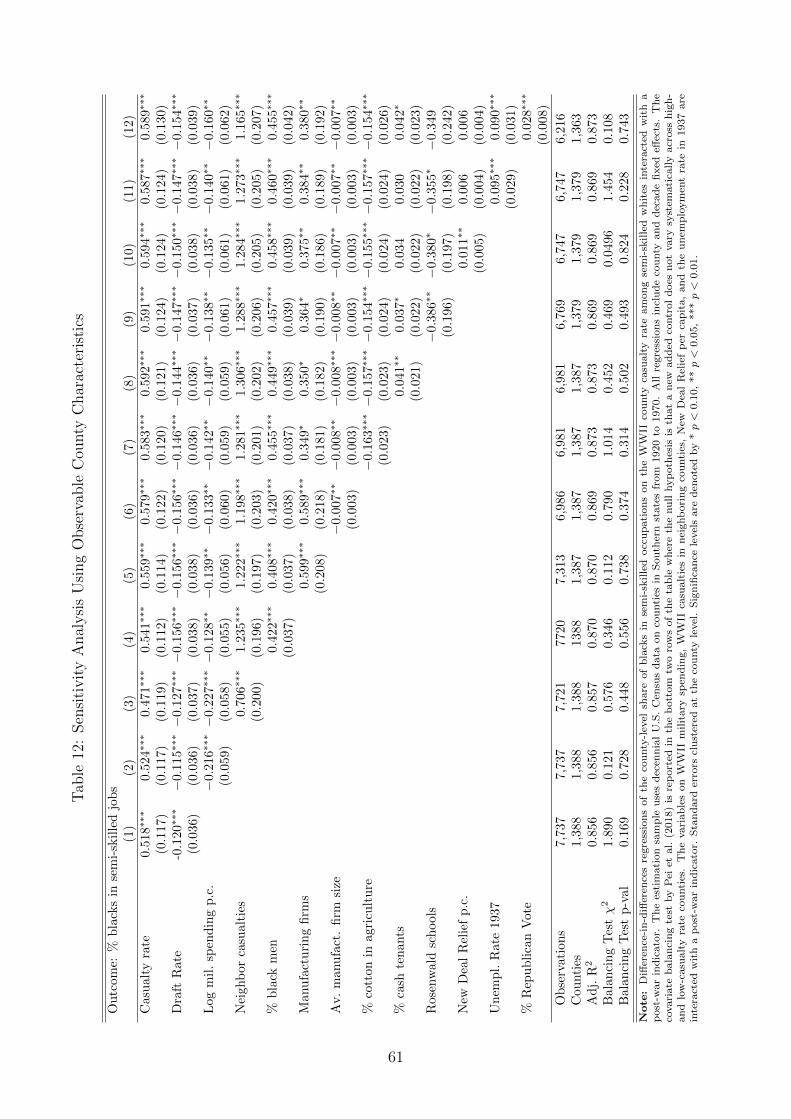
Tab

le12

:Sen

siti

vit

yA

nal

ysi

sU

sing

Obse

rvab

leC

ounty

Char

acte

rist

ics

Ou

tcom

e:%

bla

cks

inse

mi-

skil

led

job

s(1

)(2

)(3

)(4

)(5

)(6

)(7

)(8

)(9

)(1

0)

(11)

(12)

Cas

ual

tyra

te0.

518∗∗

∗0.5

24∗∗

∗0.4

71∗∗

∗0.5

41∗∗

∗0.5

59∗∗

∗0.5

79∗∗

∗0.

583∗∗

∗0.

592∗∗

∗0.

591∗∗

∗0.

594∗∗

∗0.

587∗∗

∗0.

589∗∗

∗

(0.1

17)

(0.1

17)

(0.1

19)

(0.1

12)

(0.1

14)

(0.1

22)

(0.1

20)

(0.1

21)

(0.1

24)

(0.1

24)

(0.1

24)

(0.1

30)

Dra

ftR

ate

-0.1

20∗∗

∗−

0.1

15∗∗

∗−

0.1

27∗∗

∗−

0.1

56∗∗

∗−

0.1

56∗∗

∗−

0.1

56∗∗

∗−

0.146∗∗

∗−

0.144∗∗

∗−

0.147∗∗

∗−

0.150∗∗

∗−

0.147∗∗

∗−

0.154∗∗

∗

(0.0

36)

(0.0

36)

(0.0

37)

(0.0

38)

(0.0

38)

(0.0

36)

(0.0

36)

(0.0

36)

(0.0

37)

(0.0

38)

(0.0

38)

(0.0

39)

Log

mil

.sp

end

ing

p.c

.−

0.2

16∗∗

∗−

0.2

27∗∗

∗−

0.1

28∗∗−

0.1

39∗∗−

0.1

33∗∗−

0.142∗∗−

0.140∗∗−

0.138∗∗−

0.135∗∗−

0.140∗∗−

0.160∗∗

(0.0

59)

(0.0

58)

(0.0

55)

(0.0

56)

(0.0

60)

(0.0

59)

(0.0

59)

(0.0

61)

(0.0

61)

(0.0

61)

(0.0

62)

Nei

ghb

orca

sual

ties

0.70

6∗∗∗

1.2

35∗∗

∗1.2

22∗∗

∗1.1

98∗∗

∗1.

281∗∗

∗1.

306∗∗

∗1.

288∗∗

∗1.

284∗∗

∗1.

273∗∗

∗1.

165∗∗

∗

(0.2

00)

(0.1

96)

(0.1

97)

(0.2

03)

(0.2

01)

(0.2

02)

(0.2

06)

(0.2

05)

(0.2

05)

(0.2

07)

%b

lack

men

0.4

22∗∗

∗0.4

08∗∗

∗0.4

20∗∗

∗0.4

55∗∗

∗0.

449∗∗

∗0.

457∗∗

∗0.

458∗∗

∗0.

460∗∗

∗0.

455∗∗

∗

(0.0

37)

(0.0

37)

(0.0

38)

(0.0

37)

(0.0

38)

(0.0

39)

(0.0

39)

(0.0

39)

(0.0

42)

Man

ufa

ctu

rin

gfi

rms

0.5

99∗∗

∗0.5

89∗∗

∗0.3

49∗

0.3

50∗

0.364∗

0.375∗∗

0.384∗∗

0.380∗∗

(0.2

08)

(0.2

18)

(0.1

81)

(0.1

82)

(0.1

90)

(0.1

86)

(0.1

89)

(0.1

92)

Av.

man

ufa

ct.

firm

size

−0.0

07∗∗−

0.0

08∗∗−

0.0

08∗∗

∗−

0.0

08∗∗−

0.007∗∗−

0.007∗∗−

0.007∗∗

(0.0

03)

(0.0

03)

(0.0

03)

(0.0

03)

(0.0

03)

(0.0

03)

(0.0

03)

%co

tton

inag

ricu

ltu

re−

0.1

63∗∗

∗−

0.1

57∗∗

∗−

0.1

54∗∗

∗−

0.1

55∗∗

∗−

0.157∗∗

∗−

0.154∗∗

∗

(0.0

23)

(0.0

23)

(0.0

24)

(0.0

24)

(0.0

24)

(0.0

26)

%ca

shte

nan

ts0.0

41∗∗

0.0

37∗

0.0

34

0.0

30

0.0

42∗

(0.0

21)

(0.0

22)

(0.0

22)

(0.0

22)

(0.0

23)

Ros

enw

ald

sch

ool

s−

0.3

86∗∗−

0.3

80∗−

0.3

55∗−

0.349

(0.1

96)

(0.1

97)

(0.1

98)

(0.2

42)

New

Dea

lR

elie

fp

.c.

0.0

11∗∗

0.0

06

0.0

06

(0.0

05)

(0.0

04)

(0.0

04)

Un

emp

l.R

ate

1937

0.0

95∗∗

∗0.0

90∗∗

∗

(0.0

29)

(0.0

31)

%R

epu

bli

can

Vot

e0.0

28∗∗

∗

(0.0

08)

Ob

serv

atio

ns

7,73

77,

737

7,72

17720

7,3

13

6,9

86

6,9

81

6,9

81

6,7

69

6,7

47

6,7

47

6,2

16

Cou

nti

es1,

388

1,38

81,

388

1388

1,3

87

1,3

87

1,3

87

1,3

87

1,3

79

1,3

79

1,3

79

1,3

63

Ad

j.R

20.

856

0.85

60.

857

0.8

70

0.8

70

0.8

69

0.8

73

0.8

73

0.8

69

0.8

69

0.8

69

0.8

73

Bal

anci

ng

Tes

tχ2

1.89

00.

121

0.57

60.3

46

0.1

12

0.7

90

1.0

14

0.4

52

0.4

69

0.0

496

1.4

54

0.1

08

Bal

anci

ng

Tes

tp

-val

0.16

90.

728

0.44

80.5

56

0.7

38

0.3

74

0.3

14

0.5

02

0.4

93

0.8

24

0.2

28

0.7

43

Note

:D

iffer

ence

-in

-diff

eren

ces

regre

ssio

ns

of

the

cou

nty

-lev

elsh

are

of

bla

cks

inse

mi-

skille

docc

up

ati

on

son

the

WW

IIco

unty

casu

alt

yra

team

on

gse

mi-

skille

dw

hit

esin

tera

cted

wit

ha

post

-war

ind

icato

r.T

he

esti

mati

on

sam

ple

use

sd

ecen

nia

lU

.S.

Cen

sus

data

on

cou

nti

esin

Sou

ther

nst

ate

sfr

om

1920

to1970.

All

regre

ssio

ns

incl

ud

eco

unty

an

dd

ecad

efi

xed

effec

ts.

Th

eco

vari

ate

bala

nci

ng

test

by

Pei

etal.

(2018)

isre

port

edin

the

bott

om

two

row

sof

the

tab

lew

her

eth

enu

llhyp

oth

esis

isth

at

an

ewad

ded

contr

ol

does

not

vary

syst

emati

call

yacr

oss

hig

h-

an

dlo

w-c

asu

alt

yra

teco

unti

es.

Th

evari

ab

les

on

WW

IIm

ilit

ary

spen

din

g,

WW

IIca

sualt

ies

inn

eighb

ori

ng

cou

nti

es,

New

Dea

lR

elie

fp

erca

pit

a,

an

dth

eu

nem

plo

ym

ent

rate

in1937

are

inte

ract

edw

ith

ap

ost

-war

ind

icato

r.S

tan

dard

erro

rscl

ust

ered

at

the

cou

nty

level

.S

ign

ifica

nce

level

sare

den

ote

dby

*p<

0.1

0,

**p<

0.0

5,

***p<

0.0

1.

61

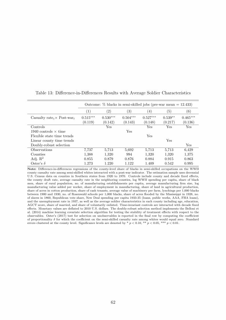
Table 13: Difference-in-Differences Results with Average Soldier Characteristics

Outcome: % blacks in semi-skilled jobs (pre-war mean = 12.433)

(1) (2) (3) (4) (5) (6)

Casualty ratec× Post-wart 0.515∗∗∗ 0.530∗∗∗ 0.504∗∗∗ 0.527∗∗∗ 0.539∗∗ 0.465∗∗∗

(0.119) (0.142) (0.143) (0.148) (0.217) (0.136)Controls Yes Yes Yes Yes1940 controls × time YesFlexible state time trends YesLinear county time trends YesDoubly-robust selection YesObservations 7,737 5,713 5,692 5,713 5,713 6,429Counties 1,388 1,320 994 1,320 1,320 1,375Adj. R2 0.855 0.879 0.876 0.884 0.915 0.863Oster’s δ 1.273 1.220 1.122 1.409 0.542 0.995

Note: Difference-in-differences regressions of the county-level share of blacks in semi-skilled occupations on the WWIIcounty casualty rate among semi-skilled whites interacted with a post-war indicator. The estimation sample uses decennialU.S. Census data on counties in Southern states from 1920 to 1970. Controls include county and decade fixed effects,the county draft rate, average casualty rate in the neighboring counties, log WWII spending per capita, share of blackmen, share of rural population, no. of manufacturing establishments per capita, average manufacturing firm size, logmanufacturing value added per worker, share of employment in manufacturing, share of land in agricultural production,share of acres in cotton production, share of cash tenants, average value of machinery per farm, lynchings per 1,000 blacksbetween 1900 and 1930, no. of Rosenwald schools per 1,000 blacks, share of acres flooded by the Mississippi in 1928, no.of slaves in 1860, Republican vote share, New Deal spending per capita 1933-35 (loans, public works, AAA, FHA loans),and the unemployment rate in 1937, as well as the average soldier characteristics in each county including age, education,AGCT score, share of married, and share of voluntarily enlisted. Time-invariant controls are interacted with decade fixedeffects. Monetary values are deflated to 2010 U.S. dollars. The doubly-robust selection method implements the Belloni etal. (2014) machine learning covariate selection algorithm for testing the stability of treatment effects with respect to theobservables. Oster’s (2017) test for selection on unobservables is reported in the final row by computing the coefficientof proportionality δ for which the coefficient on the semi-skilled casualty rate among whites would equal zero. Standarderrors clustered at the county level. Significance levels are denoted by * p < 0.10, ** p < 0.05, *** p < 0.01.

62

Table 14: Difference-in-Differences Results with Alternative Treatment Denominator

Outcome: % blacks in semi-skilled jobs (pre-war mean = 12.433)

(1) (2) (3) (4) (5) (6)

Casualty ratec× Post-wart 1.071∗∗∗ 1.770∗∗∗ 1.568∗∗∗ 1.870∗∗∗ 2.607∗∗∗ 1.962∗∗∗

(0.280) (0.386) (0.295) (0.392) (0.561) (0.349)Controls Yes Yes Yes Yes1940 controls × time YesFlexible state time trends YesLinear county time trends YesDoubly-robust selection YesObservations 7,737 5,713 5,692 5,713 5,713 6,429Counties 1,388 1,320 994 1,320 1,320 1,375Adj. R2 0.856 0.879 0.874 0.885 0.916 0.877Oster’s δ 1.946 1.514 0.953 1.487 0.853 1.568

Note: Difference-in-differences regressions of the county-level share of blacks in semi-skilled occupations on the WWIIcounty casualty rate among semi-skilled whites interacted with a post-war indicator. The casualty rate in county c hereis one hundred times the total number of killed semi-skilled whites over the number of total semi-skilled whites in 1940.The estimation sample uses decennial U.S. Census data on counties in Southern states from 1920 to 1970. Coefficients areexpressed in terms of a one standard deviation increase in the casualty rate. Controls include county and decade fixedeffects, the county draft rate, average casualty rate in the neighboring counties, log WWII spending per capita, share ofblack men, share of rural population, no. of manufacturing establishments per capita, average manufacturing firm size, logmanufacturing value added per worker, share of employment in manufacturing, share of land in agricultural production,share of acres in cotton production, share of cash tenants, average value of machinery per farm, lynchings per 1,000 blacksbetween 1900 and 1930, no. of Rosenwald schools per 1,000 blacks, share of acres flooded by the Mississippi in 1928, no.of slaves in 1860, Republican vote share, New Deal spending per capita 1933-35 (loans, public works, AAA, FHA loans),and the unemployment rate in 1937. Time-invariant controls are interacted with decade fixed effects. Monetary values aredeflated to 2010 U.S. dollars. The doubly-robust selection method implements the Belloni et al. (2014) machine learningcovariate selection algorithm for testing the stability of treatment effects with respect to the observables. Oster’s (2017)test for selection on unobservables is reported in the final row by computing the coefficient of proportionality δ for whichthe coefficient on the semi-skilled casualty rate among whites would equal zero. Standard errors clustered at the countylevel. Significance levels are denoted by * p < 0.10, ** p < 0.05, *** p < 0.01.

63

Table 15: Difference-in-Differences Results with Fixed Outcome Denominator

Outcome: % blacks in semi-skilled jobs (pre-war mean = 12.433)

(1) (2) (3) (4) (5) (6)

Casualty ratec× Post-wart 1.167∗∗∗ 1.046∗∗∗ 0.595∗∗ 0.703∗∗ 1.218∗∗ 0.345(0.283) (0.358) (0.276) (0.337) (0.538) (0.281)

Controls Yes Yes Yes Yes1940 controls × time YesFlexible state time trends YesLinear county time trends YesDoubly-robust selection YesObservations 7,737 5,713 5,692 5,713 5,713 6,429Counties 1,388 1,334 994 1,334 1,334 1,374Adj. R2 0.856 0.879 0.874 0.885 0.916 0.877Oster’s δ 1.946 1.514 0.953 1.487 0.853 1.568

Note: Difference-in-differences regressions of the county-level share of blacks in semi-skilled occupations on the WWIIcounty casualty rate among semi-skilled whites interacted with a post-war indicator. The casualty rate in county c here isone hundred times the total number of killed semi-skilled whites over the number of total semi-skilled whites in 1940. Theestimation sample uses decennial U.S. Census data on counties in Southern states from 1920 to 1970. The denominator ofthe outcome (number of semi-skilled workers) is fixed at 1940 values to reduce denominator bias. Controls include countyand decade fixed effects, the county draft rate, average casualty rate in the neighboring counties, log WWII spending percapita, share of black men, share of rural population, no. of manufacturing establishments per capita, average manufacturingfirm size, log manufacturing value added per worker, share of employment in manufacturing, share of land in agriculturalproduction, share of acres in cotton production, share of cash tenants, average value of machinery per farm, lynchings per1,000 blacks between 1900 and 1930, no. of Rosenwald schools per 1,000 blacks, share of acres flooded by the Mississippi in1928, no. of slaves in 1860, Republican vote share, New Deal spending per capita 1933-35 (loans, public works, AAA, FHAloans), and the unemployment rate in 1937. Time-invariant controls are interacted with decade fixed effects. Monetaryvalues are deflated to 2010 U.S. dollars. The doubly-robust selection method implements the Belloni et al. (2014) machinelearning covariate selection algorithm for testing the stability of treatment effects with respect to the observables. Oster’s(2017) test for selection on unobservables is reported in the final row by computing the coefficient of proportionality δ forwhich the coefficient on the semi-skilled casualty rate among whites would equal zero. Standard errors clustered at thecounty level. Significance levels are denoted by * p < 0.10, ** p < 0.05, *** p < 0.01.

64

Table 16: Difference-in-Differences Results with First Differenced Outcome

Outcome: ∆ No. of blacks in semi-sk. jobs (pre-war mean = 232.842)

(1) (2) (3) (4) (5) (6)

No. semi-sk. white deathsc 5.116∗∗∗ 4.432∗∗ 6.678∗∗ 4.295∗ 7.382 4.320∗∗∗

× Post-wart (1.779) (2.241) (3.243) (2.399) (6.757) (1.613)

Controls Yes Yes Yes Yes1940 controls × time YesFlexible state time trends YesLinear county time trends YesDoubly-robust selection YesObservations 6,006 4,677 4,513 4,677 4,677 4,687Counties 1,388 1,289 994 1,289 1,289 1,289Adj. R2 0.377 0.375 0.383 0.388 0.280 0.390

Note: Difference-in-differences regressions of the county-level share of blacks in semi-skilled occupations on the WWIIcounty casualty rate among semi-skilled whites interacted with a post-war indicator. The estimation sample uses decennialU.S. Census data on counties in Southern states from 1920 to 1970. Controls include decade fixed effects, county population,number of drafted soldiers, average casualty rate in the neighboring counties, log WWII spending per capita, share of blackmen, share of rural population, no. of manufacturing establishments per capita, average manufacturing firm size, logmanufacturing value added per worker, share of employment in manufacturing, share of land in agricultural production,share of acres in cotton production, share of cash tenants, average value of machinery per farm, lynchings per 1,000 blacksbetween 1900 and 1930, no. of Rosenwald schools per 1,000 blacks, share of acres flooded by the Mississippi in 1928, no.of slaves in 1860, Republican vote share, New Deal spending per capita 1933-35 (loans, public works, AAA, FHA loans),and the unemployment rate in 1937. Time-invariant controls are interacted with decade fixed effects. Monetary values aredeflated to 2010 U.S. dollars. The doubly-robust selection method implements the Belloni et al. (2014) machine learningcovariate selection algorithm for testing the stability of treatment effects with respect to the observables. Significance levelsare denoted by * p < 0.10, ** p < 0.05, *** p < 0.01.

65

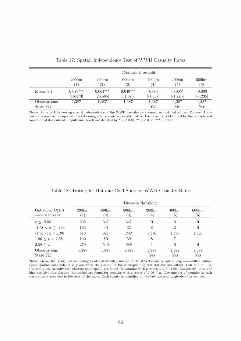
Table 17: Spatial Independence Test of WWII Casualty Rates

Distance threshold

200km 400km 600km 200km 400km 600km(1) (2) (3) (4) (5) (6)

Moran’s I 0.078∗∗∗ 0.064∗∗∗ 0.049∗∗∗ -0.008 -0.005∗ -0.003[16.473] [26.595] [31.875] [-1.557] [-1.775] [-1.235]

Observations 1,387 1,387 1,387 1,387 1,387 1,387State FE Yes Yes Yes

Note: Moran’s I for testing spatial independence of the WWII casualty rate among semi-skilled whites. For each I, thez-score is reported in squared brackets using a binary spatial weight matrix. Each county is identified by the latitude andlongitude of its centroid. Significance levels are denoted by * p < 0.10, ** p < 0.05, *** p < 0.01.

Table 18: Testing for Hot and Cold Spots of WWII Casualty Rates

Distance threshold

Getis-Ord G∗i (d) 200km 400km 600km 200km 400km 600km

z-score interval (1) (2) (3) (4) (5) (6)

z ≤ -2.58 232 347 347 0 0 0

-2.58 < z ≤ -1.96 133 49 33 8 2 0

-1.96 < z < 1.96 613 371 262 1,370 1,378 1,386

1.96 ≤ z < 2.58 130 80 59 8 7 1

2.58 ≤ z 279 540 686 1 0 0

Observations 1,387 1,387 1,387 1,387 1,387 1,387State FE Yes Yes Yes

Note: Getis-Ord G∗i (d) test for testing local spatial independence of the WWII casualty rate among semi-skilled whites.

Local spatial independence is given when the z-score on the corresponding test statistic lies within -1.96 < z < 1.96.Unusually low casualty rate clusters (cold spots) are found for counties with z-scores of z ≤ -1.96. Conversely, unusuallyhigh casualty rate clusters (hot spots) are found for counties with z-scores of 1.96 ≤ z. The number of counties in eachz-score bin is provided in the rows of the table. Each county is identified by the latitude and longitude of its centroid.

66

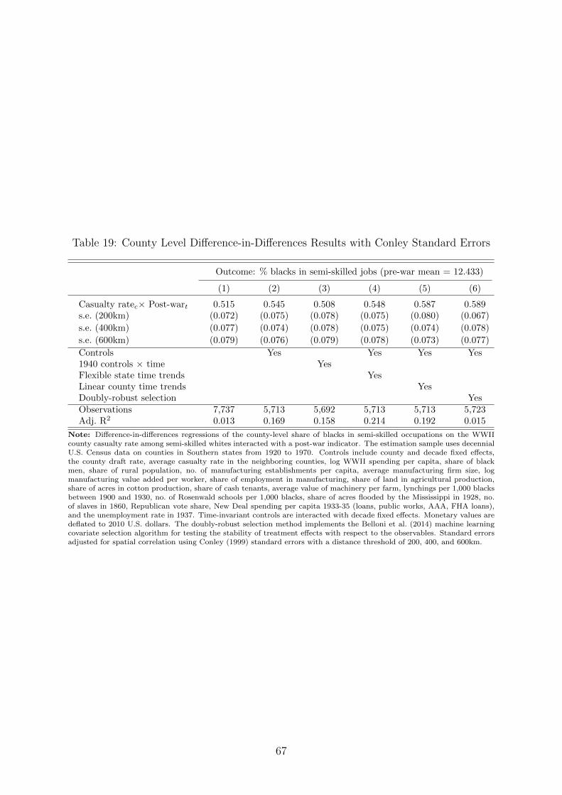
Table 19: County Level Difference-in-Differences Results with Conley Standard Errors

Outcome: % blacks in semi-skilled jobs (pre-war mean = 12.433)

(1) (2) (3) (4) (5) (6)

Casualty ratec× Post-wart 0.515 0.545 0.508 0.548 0.587 0.589s.e. (200km) (0.072) (0.075) (0.078) (0.075) (0.080) (0.067)

s.e. (400km) (0.077) (0.074) (0.078) (0.075) (0.074) (0.078)

s.e. (600km) (0.079) (0.076) (0.079) (0.078) (0.073) (0.077)

Controls Yes Yes Yes Yes1940 controls × time YesFlexible state time trends YesLinear county time trends YesDoubly-robust selection YesObservations 7,737 5,713 5,692 5,713 5,713 5,723Adj. R2 0.013 0.169 0.158 0.214 0.192 0.015

Note: Difference-in-differences regressions of the county-level share of blacks in semi-skilled occupations on the WWIIcounty casualty rate among semi-skilled whites interacted with a post-war indicator. The estimation sample uses decennialU.S. Census data on counties in Southern states from 1920 to 1970. Controls include county and decade fixed effects,the county draft rate, average casualty rate in the neighboring counties, log WWII spending per capita, share of blackmen, share of rural population, no. of manufacturing establishments per capita, average manufacturing firm size, logmanufacturing value added per worker, share of employment in manufacturing, share of land in agricultural production,share of acres in cotton production, share of cash tenants, average value of machinery per farm, lynchings per 1,000 blacksbetween 1900 and 1930, no. of Rosenwald schools per 1,000 blacks, share of acres flooded by the Mississippi in 1928, no.of slaves in 1860, Republican vote share, New Deal spending per capita 1933-35 (loans, public works, AAA, FHA loans),and the unemployment rate in 1937. Time-invariant controls are interacted with decade fixed effects. Monetary values aredeflated to 2010 U.S. dollars. The doubly-robust selection method implements the Belloni et al. (2014) machine learningcovariate selection algorithm for testing the stability of treatment effects with respect to the observables. Standard errorsadjusted for spatial correlation using Conley (1999) standard errors with a distance threshold of 200, 400, and 600km.

67

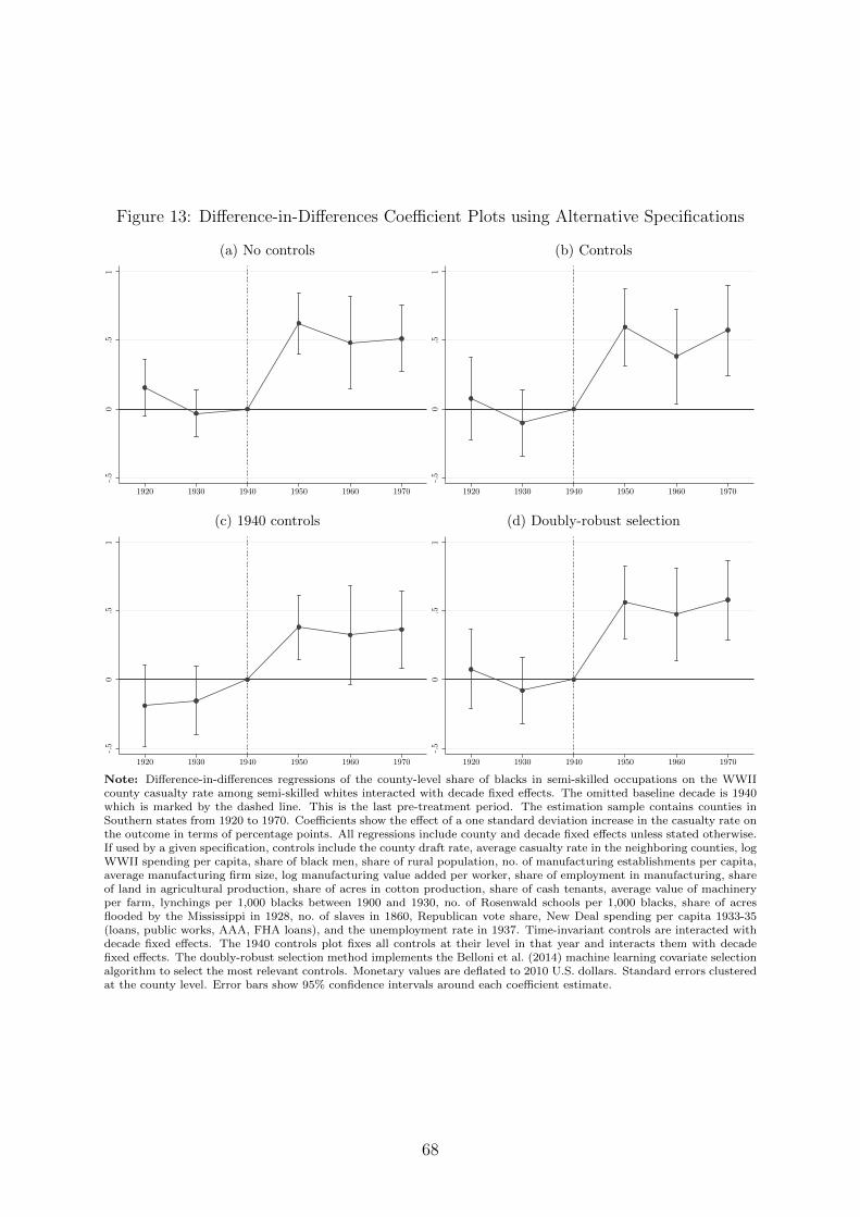
Figure 13: Difference-in-Differences Coefficient Plots using Alternative Specifications

(a) No controls

-.5

0.5

1

1920 1930 1940 1950 1960 1970

1

(b) Controls

-.5

0.5

1

1920 1930 1940 1950 1960 1970

1

(c) 1940 controls

-.5

0.5

1

1920 1930 1940 1950 1960 1970

1

(d) Doubly-robust selection

-.5

0.5

1

1920 1930 1940 1950 1960 1970

1

Note: Difference-in-differences regressions of the county-level share of blacks in semi-skilled occupations on the WWIIcounty casualty rate among semi-skilled whites interacted with decade fixed effects. The omitted baseline decade is 1940which is marked by the dashed line. This is the last pre-treatment period. The estimation sample contains counties inSouthern states from 1920 to 1970. Coefficients show the effect of a one standard deviation increase in the casualty rate onthe outcome in terms of percentage points. All regressions include county and decade fixed effects unless stated otherwise.If used by a given specification, controls include the county draft rate, average casualty rate in the neighboring counties, logWWII spending per capita, share of black men, share of rural population, no. of manufacturing establishments per capita,average manufacturing firm size, log manufacturing value added per worker, share of employment in manufacturing, shareof land in agricultural production, share of acres in cotton production, share of cash tenants, average value of machineryper farm, lynchings per 1,000 blacks between 1900 and 1930, no. of Rosenwald schools per 1,000 blacks, share of acresflooded by the Mississippi in 1928, no. of slaves in 1860, Republican vote share, New Deal spending per capita 1933-35(loans, public works, AAA, FHA loans), and the unemployment rate in 1937. Time-invariant controls are interacted withdecade fixed effects. The 1940 controls plot fixes all controls at their level in that year and interacts them with decadefixed effects. The doubly-robust selection method implements the Belloni et al. (2014) machine learning covariate selectionalgorithm to select the most relevant controls. Monetary values are deflated to 2010 U.S. dollars. Standard errors clusteredat the county level. Error bars show 95% confidence intervals around each coefficient estimate.

68

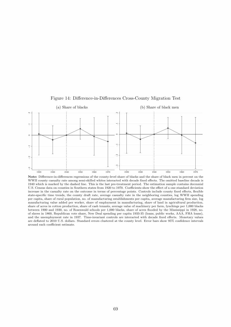
Figure 14: Difference-in-Differences Cross-County Migration Test

(a) Share of blacks

-.3

-.2

-.1

0.1

.2

1920 1930 1940 1950 1960 1970

1

(b) Share of black men

-.3

-.2

-.1

0.1

.2

1920 1930 1940 1950 1960 1970

1

Note: Difference-in-differences regressions of the county-level share of blacks and the share of black men in percent on theWWII county casualty rate among semi-skilled whites interacted with decade fixed effects. The omitted baseline decade is1940 which is marked by the dashed line. This is the last pre-treatment period. The estimation sample contains decennialU.S. Census data on counties in Southern states from 1920 to 1970. Coefficients show the effect of a one standard deviationincrease in the casualty rate on the outcome in terms of percentage points. Controls include county fixed effects, flexiblestate-specific time trends, the county draft rate, average casualty rate in the neighboring counties, log WWII spendingper capita, share of rural population, no. of manufacturing establishments per capita, average manufacturing firm size, logmanufacturing value added per worker, share of employment in manufacturing, share of land in agricultural production,share of acres in cotton production, share of cash tenants, average value of machinery per farm, lynchings per 1,000 blacksbetween 1900 and 1930, no. of Rosenwald schools per 1,000 blacks, share of acres flooded by the Mississippi in 1928, no.of slaves in 1860, Republican vote share, New Deal spending per capita 1933-35 (loans, public works, AAA, FHA loans),and the unemployment rate in 1937. Time-invariant controls are interacted with decade fixed effects. Monetary valuesare deflated to 2010 U.S. dollars. Standard errors clustered at the county level. Error bars show 95% confidence intervalsaround each coefficient estimate.

69

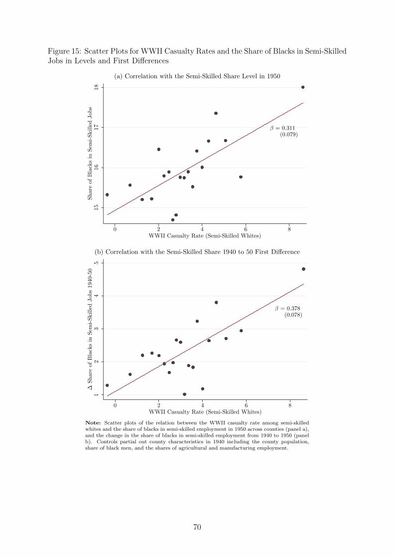
Figure 15: Scatter Plots for WWII Casualty Rates and the Share of Blacks in Semi-SkilledJobs in Levels and First Differences

(a) Correlation with the Semi-Skilled Share Level in 1950

β = 0.311(0.079)

1516

1718

Shareof

Blacksin

Sem

i-SkilledJob

s

0 2 4 6 8WWII Casualty Rate (Semi-Skilled Whites)

1

(b) Correlation with the Semi-Skilled Share 1940 to 50 First Difference

β = 0.378(0.078)

13

5∆

Shareof

Blacksin

Sem

i-SkilledJob

s1940-50

0 2

2

4

4

6 8WWII Casualty Rate (Semi-Skilled Whites)

1

Note: Scatter plots of the relation between the WWII casualty rate among semi-skilledwhites and the share of blacks in semi-skilled employment in 1950 across counties (panel a),and the change in the share of blacks in semi-skilled employment from 1940 to 1950 (panelb). Controls partial out county characteristics in 1940 including the county population,share of black men, and the shares of agricultural and manufacturing employment.

70

Figure 16: Difference-in-Differences Coefficient Plot with Alternative Treatment

-10

12

3

1920 1930 1940 1950 1960 1970

1

Note: Difference-in-differences regressions of the county-level share of blacks in semi-skilled occupations on the WWIIcounty casualty rate among semi-skilled whites interacted with decade fixed effects. The denominator in the computationof the casualty rate here is the number of all semi-skilled whites in 1940 in county c. The omitted baseline decade is 1940which is marked by the dashed line. This is the last pre-treatment period. The estimation sample contains counties inSouthern states from 1920 to 1970. Coefficients show the effect of a one standard deviation increase in the casualty rate onthe outcome in terms of percentage points. Controls include county and decade fixed effects, the county draft rate, averagecasualty rate in the neighboring counties, log WWII spending per capita, share of black men, share of rural population, no.of manufacturing establishments per capita, average manufacturing firm size, log manufacturing value added per worker,share of employment in manufacturing, share of land in agricultural production, share of acres in cotton production, shareof cash tenants, average value of machinery per farm, lynchings per 1,000 blacks between 1900 and 1930, no. of Rosenwaldschools per 1,000 blacks, share of acres flooded by the Mississippi in 1928, no. of slaves in 1860, Republican vote share,New Deal spending per capita 1933-35 (loans, public works, AAA, FHA loans), and the unemployment rate in 1937. Time-invariant controls are interacted with decade fixed effects. Monetary values are deflated to 2010 U.S. dollars. Standarderrors clustered at the county level. Error bars show 95% confidence intervals around each coefficient estimate.

71

Figure 17: Voluntary Enlistment Rates

(a) South vs. Non-South0

2040

6080

100

EnlistmentShareof

Total

Entries

1940 1941 1942 1943 1944 1945 1946

South Non-South

1

(b) Within South

0.2

.4.6

.81

Shareof

Voluntary

Enlistments

per

Mon

th

July 1940 July 1941 July 1942 July 1943 July 1944 July 1945

Below Median Casualties Above Median Casualties

1

Note: Share of voluntary enlistments out of total new entries into the Army and Army Air Force by month. The drop atthe end of 1942 is because voluntary enlistment was forbidden to avoid hurting the war economy due to overenthusiasticenlistments as was the case in the United Kingdom. After December 1942 only men aged 38 or older were allowed tovolunteer if they demonstrated their physical and mental fitness for service.

72

Figure 18: Leave-One Out DiD Sensitivity CheckPSfrag

Alabama

Arkansas

Delaware

D.C.

Florida

Georgia

Kentucky

Louisiana

Maryland

Mississippi

N. Carolina

Oklahoma

S. Carolina

Tennessee

Texas

Virginia

W. Virginia

0 .2 .4 .6 .8 1Casualty Rate DiD Coefficient

Left-out State:

1

Note: Difference-in-differences regressions of the county-level share of blacks in semi-skilled occupations on the WWIIcounty casualty rate among semi-skilled whites interacted with a post-war indicator. The estimation sample uses decennialU.S. Census data on counties in Southern states from 1920 to 1970. Each regression leaves out all counties from a specificstate at a time to assess whether results are driven by any one single state. The omitted state is listed on the left. Eachregression includes county and decade fixed effects, the county draft rate, average casualty rate in the neighboring counties,log WWII spending per capita, share of black men, share of rural population, no. of manufacturing establishments percapita, average manufacturing firm size, log manufacturing value added per worker, share of employment in manufacturing,share of land in agricultural production, share of acres in cotton production, share of cash tenants, average value ofmachinery per farm, lynchings per 1,000 blacks between 1900 and 1930, no. of Rosenwald schools per 1,000 blacks, share ofacres flooded by the Mississippi in 1928, no. of slaves in 1860, Republican vote share, New Deal spending per capita 1933-35(loans, public works, AAA, FHA loans), and the unemployment rate in 1937. Time-invariant controls are interacted withdecade fixed effects. Monetary values are deflated to 2010 U.S. dollars. Standard errors are clustered by county. Error barsshow 95% confidence intervals.

73

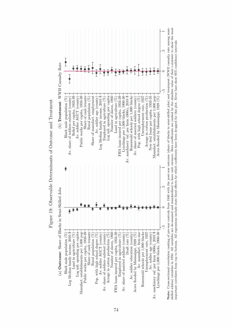
Fig

ure

19:

Obse

rvab

leD

eter

min

ants

ofO

utc

ome

and

Tre

atm

ent

(a)Outcome:

Sh

are

ofB

lack

sin

Sem

i-S

kil

led

Job

s

Black

malepop

ulation

(%)

Log

Med

ianfamilyincome,

2010

$Lan

din

agricu

lture

(%)

Log

mil.spen

dingper

capita

Man

ufact.establishments

per

1,000pop

Publicworksper

capita,

1933-39

Shareof

cash

tenan

tsRuralpop

ulation

(%)

Pop

.withhighschool

degree(%

)Av.soldierAGCT

(cou

nty)

Av.shareof

soldiers

enlisted

(cou

nty)

Acragein

cotton

production(%

)Number

ofslaves,1860

FHA

loan

sinsuredper

capita,

1934-39

Employedin

agricu

lture

(%)

Av.shareof

married

soldiers

(cou

nty)

Draft

rate

(%)

Av.soldiered

ucation

(cou

nty)

Acres

flooded

byMississippi,1928

(%)

Av.man

ufact.firm

size

Rosenwaldschoolsper

1,000blacks

Unem

ploymentrate,1937

Av.soldierage(cou

nty)

Av.machineryval.per

farm

(000s),2010

$Lynchings

per

1,000blacks,

1900-30

-.5

0.5

1

1

(b)Tre

atm

ent:

WW

IIC

asu

alt

yR

ate

Black

malepop

ulation

(%)

Av.shareof

soldiers

enlisted

(cou

nty)

Reliefper

capita,

1933-39

Av.soldierAGCT

(cou

nty)

Publicworksper

capita,

1933-39

Shareof

cash

tenan

tsRuralpop

ulation

(%)

Shareof

man

ufact.em

ployment

Av.soldierage(cou

nty)

Log

Med

ianfamilyincome,

2010

$Employedin

agricu

lture

(%)

Log

mil.spen

dingper

capita

Number

ofslaves,1860

Lan

din

agricu

lture

(%)

FHA

loan

sinsuredper

capita,

1934-39

Lynchings

per

1,000blacks,

1900-30

Av.machineryval.per

farm

(000s),2010

$Rosenwaldschoolsper

1,000blacks

Av.shareof

married

soldiers

(cou

nty)

Pop

.withhighschool

degree(%

)Unem

ploymentrate,1937

Acragein

cotton

production(%

)New

dealloan

sper

capita,

1933-35

Man

ufact.establishments

per

1,000pop

Acres

flooded

byMississippi,1928

(%)

-.5

0.5

1

1

Note

:C

ross

-sec

tion

al

corr

elati

on

ran

kin

gof

pre

-war

contr

ols

from

1940

wit

hth

ep

ost

-war

ou

tcom

e(s

hare

of

bla

cks

inse

mi-

skille

djo

bs)

an

dtr

eatm

ent

(WW

IIca

sualt

yra

team

on

gse

mi-

skille

dw

hit

es)

vari

ab

les

in1950.

All

vari

ab

les

are

de-

mea

ned

an

dst

an

dard

ized

toh

ave

un

itvari

an

ce.

Bet

aco

effici

ents

are

ran

ked

by

the

ab

solu

tevalu

eof

thei

rt-

stati

stic

tosh

ow

the

most

imp

ort

ant

corr

elate

sfr

om

top

tob

ott

om

.A

llre

gre

ssio

ns

incl

ud

est

ate

fixed

effec

tsfo

rw

hic

hco

effici

ents

have

bee

nd

rop

ped

for

this

plo

t.E

rror

bars

show

95%

con

fid

ence

inte

rvals

.

74

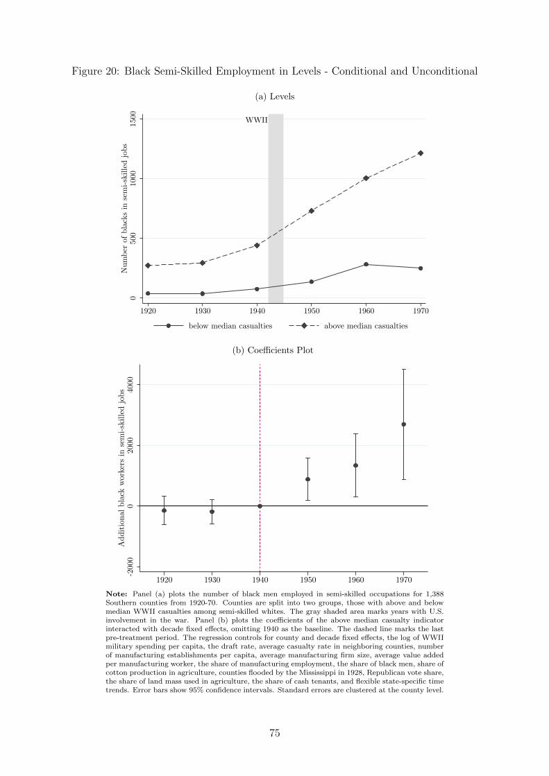
Figure 20: Black Semi-Skilled Employment in Levels - Conditional and Unconditional

(a) Levels

WWII

0500

1000

1500

Number

ofblacksin

semi-skilledjobs

1920 1930 1940 1950 1960 1970

below median casualties above median casualties

1

(b) Coefficients Plot

-2000

02000

4000

Additional

black

workers

insemi-skilledjobs

1920 1930 1940 1950 1960 1970

1

Note: Panel (a) plots the number of black men employed in semi-skilled occupations for 1,388Southern counties from 1920-70. Counties are split into two groups, those with above and belowmedian WWII casualties among semi-skilled whites. The gray shaded area marks years with U.S.involvement in the war. Panel (b) plots the coefficients of the above median casualty indicatorinteracted with decade fixed effects, omitting 1940 as the baseline. The dashed line marks the lastpre-treatment period. The regression controls for county and decade fixed effects, the log of WWIImilitary spending per capita, the draft rate, average casualty rate in neighboring counties, numberof manufacturing establishments per capita, average manufacturing firm size, average value addedper manufacturing worker, the share of manufacturing employment, the share of black men, share ofcotton production in agriculture, counties flooded by the Mississippi in 1928, Republican vote share,the share of land mass used in agriculture, the share of cash tenants, and flexible state-specific timetrends. Error bars show 95% confidence intervals. Standard errors are clustered at the county level.

75

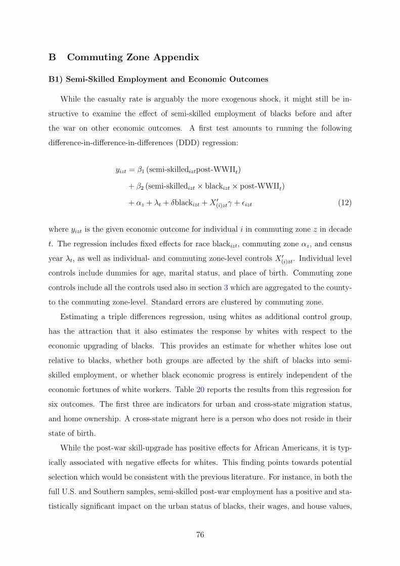
B Commuting Zone Appendix

B1) Semi-Skilled Employment and Economic Outcomes

While the casualty rate is arguably the more exogenous shock, it might still be in-

structive to examine the effect of semi-skilled employment of blacks before and after

the war on other economic outcomes. A first test amounts to running the following

difference-in-difference-in-differences (DDD) regression:

yizt = β1 (semi-skillediztpost-WWIIt)

+ β2 (semi-skilledizt × blackizt × post-WWIIt)

+ αz + λt + δblackizt +X ′(i)ztγ + εizt (12)

where yizt is the given economic outcome for individual i in commuting zone z in decade

t. The regression includes fixed effects for race blackizt, commuting zone αz, and census

year λt, as well as individual- and commuting zone-level controls X ′(i)zt. Individual level

controls include dummies for age, marital status, and place of birth. Commuting zone

controls include all the controls used also in section 3 which are aggregated to the county-

to the commuting zone-level. Standard errors are clustered by commuting zone.

Estimating a triple differences regression, using whites as additional control group,

has the attraction that it also estimates the response by whites with respect to the

economic upgrading of blacks. This provides an estimate for whether whites lose out

relative to blacks, whether both groups are affected by the shift of blacks into semi-

skilled employment, or whether black economic progress is entirely independent of the

economic fortunes of white workers. Table 20 reports the results from this regression for

six outcomes. The first three are indicators for urban and cross-state migration status,

and home ownership. A cross-state migrant here is a person who does not reside in their

state of birth.

While the post-war skill-upgrade has positive effects for African Americans, it is typ-

ically associated with negative effects for whites. This finding points towards potential

selection which would be consistent with the previous literature. For instance, in both the

full U.S. and Southern samples, semi-skilled post-war employment has a positive and sta-

tistically significant impact on the urban status of blacks, their wages, and house values,

76

but affects whites in the opposite direction. Boustan (2010) shows that for every black

arrival into a Northern city center 2.7 whites leave. If the more skilled or wealthy whites

can more easily switch jobs or their homes, then the remaining whites are a selected part

of the white population that was too constrained to satisfy their racial preferences - or

that was more tolerant to begin with.

Blacks who secure a semi-skilled job after the war are looking at a substantial wage

increase of 28.4 p.p. in the full sample and 33.2 p.p. in the Southern sample. The skill-

upgrade is only significantly related to the probability of home ownership in the full

sample with a 1.2 p.p. rise. However, when African Americans manage to own their home,

this is now of substantially higher value for those who experience the skill-upgrade. The

associated home value increase is 30.9 p.p. in the whole U.S. and 41.1 p.p. in the South.

For whites there is a negative effect on house values which might be due to outmigration

of wealthier whites driving down home values (Boustan and Margo, 2013) or a decline in

housing segregation that reduces prices for homes of whites (Logan and Parman, 2017).

77

Table 20: Micro Census Triple Differences Results using the Semi-Skilled Treatment

Outcome: ln(wage) Education Owns home ln(house val.) Migrant

Panel A: All U.S.

Semi-Skilledizt× Post-wart -0.072∗∗∗ -1.832∗∗∗ -0.001 -0.246∗∗∗ -0.013∗∗

(0.007) (0.035) (0.003) (0.005) (0.006)

Semi-Skilledizt× Blackizt× 0.250∗∗∗ 1.757∗∗∗ 0.012∗ 0.269∗∗∗ 0.015∗∗

Post-wart (0.010) (0.054) (0.007) (0.015) (0.008)

Observations 2,696,784 3,119,306 4,211,898 1,527,493 4,335,995Adj. R2 0.502 0.457 0.251 0.487 0.323

Panel B: South Only

Semi-Skilledizt× Post-wart -0.100∗∗∗ -1.843∗∗∗ -0.012∗∗ -0.309∗∗∗ 0.014(0.014) (0.069) (0.005) (0.011) (0.009)

Semi-Skilledizt× Blackizt× 0.288∗∗∗ 1.902∗∗∗ 0.009 0.344∗∗∗ -0.015∗∗

Post-wart (0.013) (0.078) (0.006) (0.019) (0.006)

Observations 766,766 910,755 1,226,713 428,483 1,268,890Adj. R2 0.507 0.452 0.241 0.508 0.467

Note: Difference-in-differenece-in-differences regression of economic outcomes on the commuting zone WWII casualty rateamong semi-skilled whites interacted with a post-WWII dummy, and with a black indicator for individuals living in 722commuting zones in the whole U.S. The estimation sample contains data from the decennial U.S. micro Census from 1920-70on non-institutionalized, working black and white males aged 15-65 who are not currently attending school. All regressionsinclude commuting zone and Census year fixed effects. Owns home is a binary outcome for whether an individual owns theirhome. The log house value, log wages, and education variables are only available from 1940 onward. Log house value is alsomissing for 1950. Individual level controls include age, marital status, age and place of birth dummies. Commuting zonelevel controls are the WWII draft rate, log WWII spending per capita, share of black men, share of rural population, no.of manufacturing establishments per capita, average manufacturing firm size, log manufacturing value added per worker,share of employment in manufacturing, share of land in agricultural production, share of acres in cotton production, shareof cash tenants, average value of machinery per farm, lynchings per 1,000 blacks between 1900 and 1930, no. of Rosenwaldschools per 1,000 blacks, share of acres flooded by the Mississippi in 1928, no. of slaves in 1860, Republican vote share,New Deal spending per capita 1933-35 (loans, public works, AAA, FHA loans), and the unemployment rate in 1937. Time-invariant controls are interacted with decade fixed effects. Monetary values are deflated to 2010 U.S. dollars. Standarderrors clustered at the commuting zone level in parentheses. Significance levels are denoted by * p < 0.10, ** p < 0.05, ***p < 0.01.

78

B2) Further Robustness Checks for Migration Responses

Are the results here driven by migration? To test for this possibility, tables 21 and 22

repeat the DDD analysis for the sub-samples of those who do not reside in their state of

birth and birth-state stayers in the country as a whole and in the South only, respectively.

While wage gains are typically larger for those who move, the casualty rate effect increases

the house values only for birth-state stayers in the full sample. The likely reason for this

relates to blacks moving to lower quality housing in the city centers of the industrial

centers in the North. When considering the Southern sample, movers also outperform

stayers in terms of house value. This difference is not statistically significant though.

Even though moving is an endogenous choice, the results here provide evidence that the

economic benefits are not only reaped by this particular group of individuals. Also stayers

gain. Even though the wage increases associated with the white WWII casualty rate are

lower for stayers, the increases in house value and educational attainment are comparable

across movers and stayers.

79

Table 21: Movers vs. Birth-State Stayers, all U.S.

Outcome: ln(wage) Education Owns home ln(house value)

Panel A: Cross-State Migrants

Casualty ratez× Post-wart -0.022∗∗ -0.030 0.000 -0.051∗∗

(0.010) (0.037) (0.005) (0.021)

Casualty ratez× Blackizt× 0.055∗∗∗ 0.240∗∗∗ 0.004 0.025Post-wart (0.006) (0.032) (0.005) (0.020)

Observations 1,073,820 1,208,270 1,515,175 557,437Adj. R2 0.462 0.409 0.263 0.430

Panel B: Birth-State Stayers

Casualty ratez× Post-wart -0.012 -0.033 -0.007∗ -0.033(0.009) (0.029) (0.004) (0.022)

Casualty ratez× Blackizt× 0.027∗∗∗ 0.311∗∗∗ -0.012∗∗∗ 0.084∗∗∗

Post-wart (0.007) (0.028) (0.003) (0.010)

Observations 1,622,964 1,911,036 2,696,723 970,056Adj. R2 0.523 0.453 0.255 0.492

Note: Difference-in-differenece-in-differences regression of economic outcomes on the commuting zone WWII casualty rateamong semi-skilled whites interacted with a post-WWII dummy, and with a black indicator for individuals living in 722commuting zones in the whole U.S. The estimation sample contains data from the decennial U.S. micro Census from 1920-70on non-institutionalized, working black and white males aged 15-65 who are not currently attending school. All regressionsinclude commuting zone and Census year fixed effects. Owns home is a binary outcome for whether an individual owns theirhome. The log house value, log wages, and education variables are only available from 1940 onward. Log house value is alsomissing for 1950. Individual level controls include age, marital status, age and place of birth dummies. Commuting zonelevel controls are the WWII draft rate, log WWII spending per capita, share of black men, share of rural population, no.of manufacturing establishments per capita, average manufacturing firm size, log manufacturing value added per worker,share of employment in manufacturing, share of land in agricultural production, share of acres in cotton production, shareof cash tenants, average value of machinery per farm, lynchings per 1,000 blacks between 1900 and 1930, no. of Rosenwaldschools per 1,000 blacks, share of acres flooded by the Mississippi in 1928, no. of slaves in 1860, Republican vote share,New Deal spending per capita 1933-35 (loans, public works, AAA, FHA loans), and the unemployment rate in 1937. Time-invariant controls are interacted with decade fixed effects. Monetary values are deflated to 2010 U.S. dollars. Standarderrors clustered at the commuting zone level in parentheses. Significance levels are denoted by * p < 0.10, ** p < 0.05, ***p < 0.01.

80

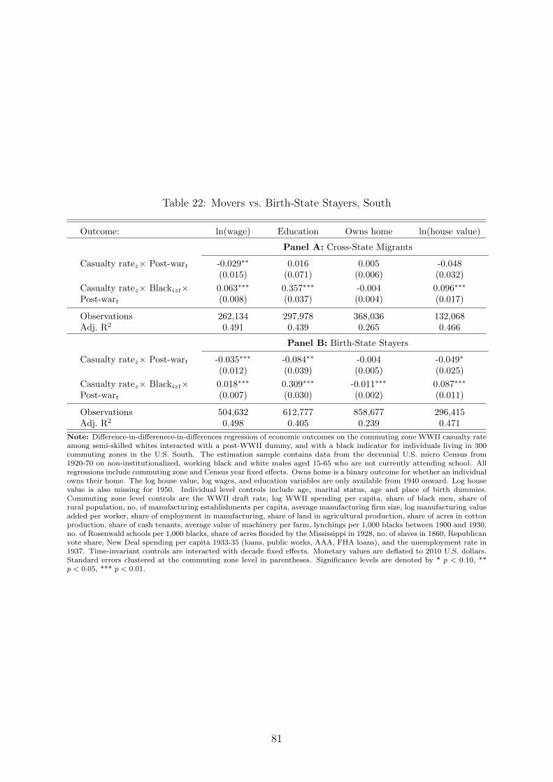
Table 22: Movers vs. Birth-State Stayers, South

Outcome: ln(wage) Education Owns home ln(house value)

Panel A: Cross-State Migrants

Casualty ratez× Post-wart -0.029∗∗ 0.016 0.005 -0.048(0.015) (0.071) (0.006) (0.032)

Casualty ratez× Blackizt× 0.063∗∗∗ 0.357∗∗∗ -0.004 0.096∗∗∗

Post-wart (0.008) (0.037) (0.004) (0.017)

Observations 262,134 297,978 368,036 132,068Adj. R2 0.491 0.439 0.265 0.466

Panel B: Birth-State Stayers

Casualty ratez× Post-wart -0.035∗∗∗ -0.084∗∗ -0.004 -0.049∗

(0.012) (0.039) (0.005) (0.025)

Casualty ratez× Blackizt× 0.018∗∗∗ 0.309∗∗∗ -0.011∗∗∗ 0.087∗∗∗

Post-wart (0.007) (0.030) (0.002) (0.011)

Observations 504,632 612,777 858,677 296,415Adj. R2 0.498 0.405 0.239 0.471

Note: Difference-in-differenece-in-differences regression of economic outcomes on the commuting zone WWII casualty rateamong semi-skilled whites interacted with a post-WWII dummy, and with a black indicator for individuals living in 300commuting zones in the U.S. South. The estimation sample contains data from the decennial U.S. micro Census from1920-70 on non-institutionalized, working black and white males aged 15-65 who are not currently attending school. Allregressions include commuting zone and Census year fixed effects. Owns home is a binary outcome for whether an individualowns their home. The log house value, log wages, and education variables are only available from 1940 onward. Log housevalue is also missing for 1950. Individual level controls include age, marital status, age and place of birth dummies.Commuting zone level controls are the WWII draft rate, log WWII spending per capita, share of black men, share ofrural population, no. of manufacturing establishments per capita, average manufacturing firm size, log manufacturing valueadded per worker, share of employment in manufacturing, share of land in agricultural production, share of acres in cottonproduction, share of cash tenants, average value of machinery per farm, lynchings per 1,000 blacks between 1900 and 1930,no. of Rosenwald schools per 1,000 blacks, share of acres flooded by the Mississippi in 1928, no. of slaves in 1860, Republicanvote share, New Deal spending per capita 1933-35 (loans, public works, AAA, FHA loans), and the unemployment rate in1937. Time-invariant controls are interacted with decade fixed effects. Monetary values are deflated to 2010 U.S. dollars.Standard errors clustered at the commuting zone level in parentheses. Significance levels are denoted by * p < 0.10, **p < 0.05, *** p < 0.01.

81

C NPPS Additional Results

C1) Robustness and Heterogeneity

C1.1: Splitting the Sample into Black and White Respondents

Tables 23 and 24 re-estimate the OLS and IV regressions for eq. (6) for the black and

white samples, respectively. Given that the sample size is essentially halved, this is

reflected in the very wide standard errors. The main aim of this exercise is to explore

from which group the estimated effect sizes in the main table originate. In most cases

the absolute size of the coefficients is larger in the sample of black respondents. However,

comparing the coefficients to the sample means within each group shows that the relative

magnitudes are comparable across blacks and whites. The only outcome where black and

white respondents differ is the favor integration at church outcome which yields a slightly

negative but close to zero IV coefficient for whites. This is the only result which is mainly

driven by black respondents.

C1.2: Weighted Regressions

Despite the attempt by the authors of the initial study to produce a representative sample

of the Southern population, blacks and whites were sampled in equal proportion. This

does not reflect the population shares in their counties of residence. To account for this,

table 25 weights black and white respondents by their population share in their residence

county. This does not overturn the previous findings.

C1.3: Alternative Treatment Definition

Another concern is that the treatment change from 1940 to 1950 is not relevant for black-

white social outcomes in 1961. I therefore re-estimate eq. (6) by taking the change from

1940 to 1960. While the instrument does gain strength, the point estimates are not

significantly different from the main results. The results from this exercise are reported

in table 26

82

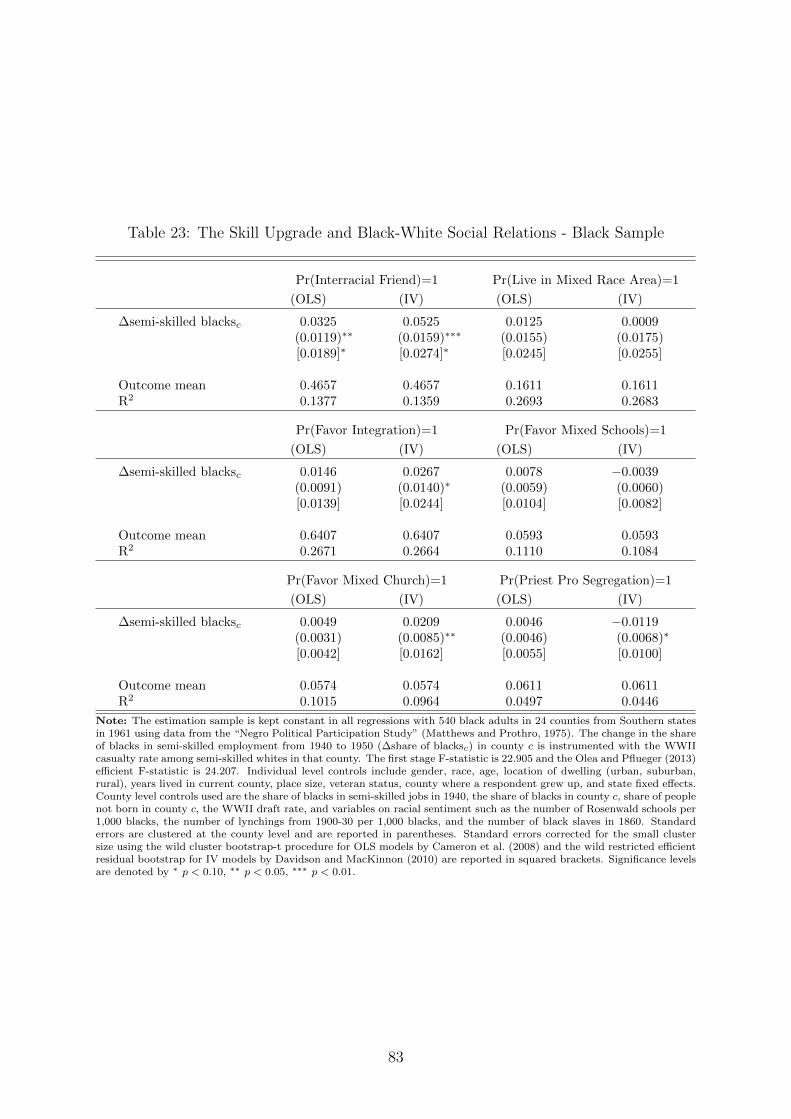
Table 23: The Skill Upgrade and Black-White Social Relations - Black Sample

Pr(Interracial Friend)=1 Pr(Live in Mixed Race Area)=1

(OLS) (IV) (OLS) (IV)

∆semi-skilled blacksc 0.0325 0.0525 0.0125 0.0009(0.0119)∗∗ (0.0159)∗∗∗ (0.0155) (0.0175)[0.0189]∗ [0.0274]∗ [0.0245] [0.0255]

Outcome mean 0.4657 0.4657 0.1611 0.1611R2 0.1377 0.1359 0.2693 0.2683

Pr(Favor Integration)=1 Pr(Favor Mixed Schools)=1

(OLS) (IV) (OLS) (IV)

∆semi-skilled blacksc 0.0146 0.0267 0.0078 −0.0039(0.0091) (0.0140)∗ (0.0059) (0.0060)[0.0139] [0.0244] [0.0104] [0.0082]

Outcome mean 0.6407 0.6407 0.0593 0.0593R2 0.2671 0.2664 0.1110 0.1084

Pr(Favor Mixed Church)=1 Pr(Priest Pro Segregation)=1

(OLS) (IV) (OLS) (IV)

∆semi-skilled blacksc 0.0049 0.0209 0.0046 −0.0119(0.0031) (0.0085)∗∗ (0.0046) (0.0068)∗

[0.0042] [0.0162] [0.0055] [0.0100]

Outcome mean 0.0574 0.0574 0.0611 0.0611R2 0.1015 0.0964 0.0497 0.0446

Note: The estimation sample is kept constant in all regressions with 540 black adults in 24 counties from Southern statesin 1961 using data from the “Negro Political Participation Study” (Matthews and Prothro, 1975). The change in the shareof blacks in semi-skilled employment from 1940 to 1950 (∆share of blacksc) in county c is instrumented with the WWIIcasualty rate among semi-skilled whites in that county. The first stage F-statistic is 22.905 and the Olea and Pflueger (2013)efficient F-statistic is 24.207. Individual level controls include gender, race, age, location of dwelling (urban, suburban,rural), years lived in current county, place size, veteran status, county where a respondent grew up, and state fixed effects.County level controls used are the share of blacks in semi-skilled jobs in 1940, the share of blacks in county c, share of peoplenot born in county c, the WWII draft rate, and variables on racial sentiment such as the number of Rosenwald schools per1,000 blacks, the number of lynchings from 1900-30 per 1,000 blacks, and the number of black slaves in 1860. Standarderrors are clustered at the county level and are reported in parentheses. Standard errors corrected for the small clustersize using the wild cluster bootstrap-t procedure for OLS models by Cameron et al. (2008) and the wild restricted efficientresidual bootstrap for IV models by Davidson and MacKinnon (2010) are reported in squared brackets. Significance levelsare denoted by ∗ p < 0.10, ∗∗ p < 0.05, ∗∗∗ p < 0.01.

83

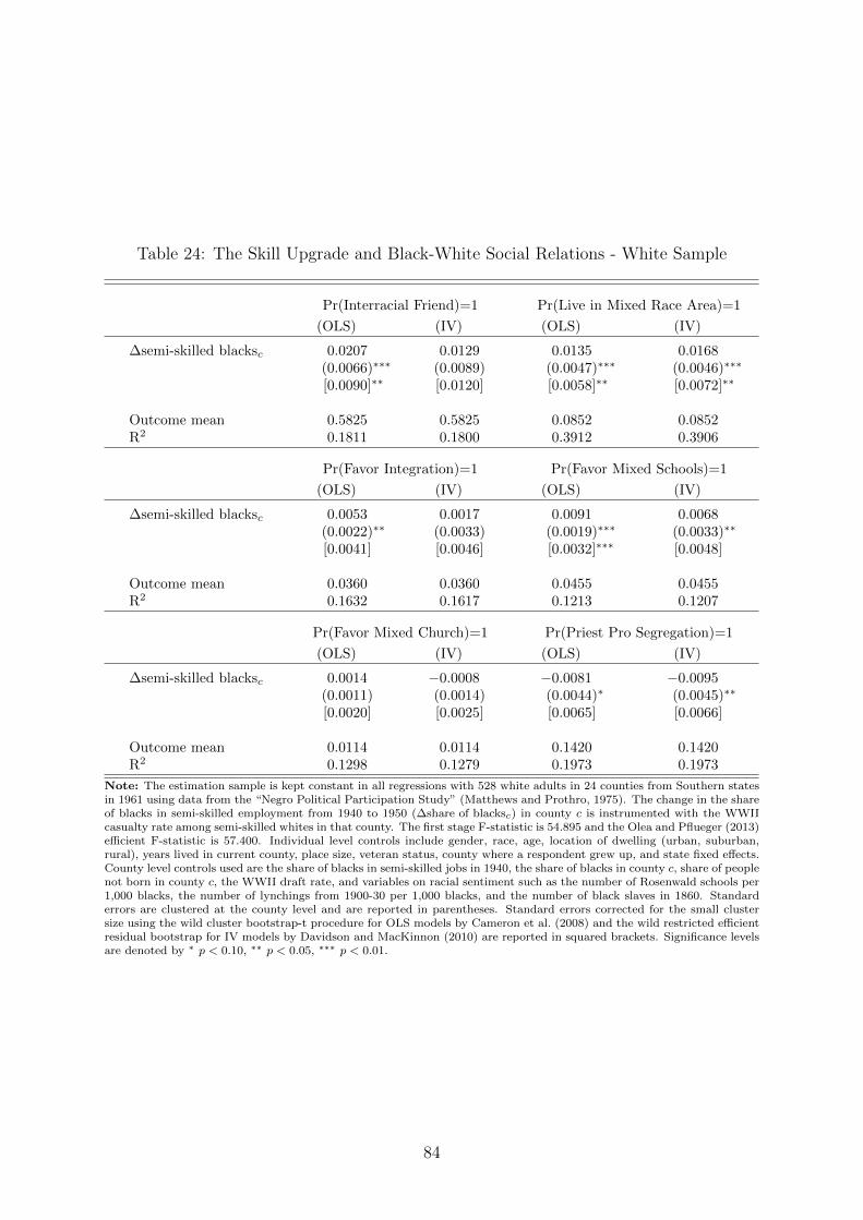
Table 24: The Skill Upgrade and Black-White Social Relations - White Sample

Pr(Interracial Friend)=1 Pr(Live in Mixed Race Area)=1

(OLS) (IV) (OLS) (IV)

∆semi-skilled blacksc 0.0207 0.0129 0.0135 0.0168(0.0066)∗∗∗ (0.0089) (0.0047)∗∗∗ (0.0046)∗∗∗

[0.0090]∗∗ [0.0120] [0.0058]∗∗ [0.0072]∗∗

Outcome mean 0.5825 0.5825 0.0852 0.0852R2 0.1811 0.1800 0.3912 0.3906

Pr(Favor Integration)=1 Pr(Favor Mixed Schools)=1

(OLS) (IV) (OLS) (IV)

∆semi-skilled blacksc 0.0053 0.0017 0.0091 0.0068(0.0022)∗∗ (0.0033) (0.0019)∗∗∗ (0.0033)∗∗

[0.0041] [0.0046] [0.0032]∗∗∗ [0.0048]

Outcome mean 0.0360 0.0360 0.0455 0.0455R2 0.1632 0.1617 0.1213 0.1207

Pr(Favor Mixed Church)=1 Pr(Priest Pro Segregation)=1

(OLS) (IV) (OLS) (IV)

∆semi-skilled blacksc 0.0014 −0.0008 −0.0081 −0.0095(0.0011) (0.0014) (0.0044)∗ (0.0045)∗∗

[0.0020] [0.0025] [0.0065] [0.0066]

Outcome mean 0.0114 0.0114 0.1420 0.1420R2 0.1298 0.1279 0.1973 0.1973

Note: The estimation sample is kept constant in all regressions with 528 white adults in 24 counties from Southern statesin 1961 using data from the “Negro Political Participation Study” (Matthews and Prothro, 1975). The change in the shareof blacks in semi-skilled employment from 1940 to 1950 (∆share of blacksc) in county c is instrumented with the WWIIcasualty rate among semi-skilled whites in that county. The first stage F-statistic is 54.895 and the Olea and Pflueger (2013)efficient F-statistic is 57.400. Individual level controls include gender, race, age, location of dwelling (urban, suburban,rural), years lived in current county, place size, veteran status, county where a respondent grew up, and state fixed effects.County level controls used are the share of blacks in semi-skilled jobs in 1940, the share of blacks in county c, share of peoplenot born in county c, the WWII draft rate, and variables on racial sentiment such as the number of Rosenwald schools per1,000 blacks, the number of lynchings from 1900-30 per 1,000 blacks, and the number of black slaves in 1860. Standarderrors are clustered at the county level and are reported in parentheses. Standard errors corrected for the small clustersize using the wild cluster bootstrap-t procedure for OLS models by Cameron et al. (2008) and the wild restricted efficientresidual bootstrap for IV models by Davidson and MacKinnon (2010) are reported in squared brackets. Significance levelsare denoted by ∗ p < 0.10, ∗∗ p < 0.05, ∗∗∗ p < 0.01.

84

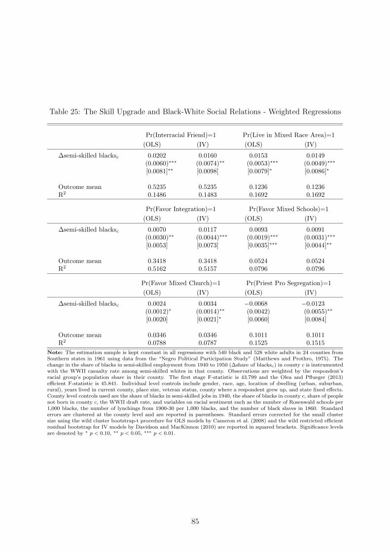
Table 25: The Skill Upgrade and Black-White Social Relations - Weighted Regressions

Pr(Interracial Friend)=1 Pr(Live in Mixed Race Area)=1

(OLS) (IV) (OLS) (IV)

∆semi-skilled blacksc 0.0202 0.0160 0.0153 0.0149(0.0060)∗∗∗ (0.0074)∗∗ (0.0053)∗∗∗ (0.0049)∗∗∗

[0.0081]∗∗ [0.0098] [0.0079]∗ [0.0086]∗

Outcome mean 0.5235 0.5235 0.1236 0.1236R2 0.1486 0.1483 0.1692 0.1692

Pr(Favor Integration)=1 Pr(Favor Mixed Schools)=1

(OLS) (IV) (OLS) (IV)

∆semi-skilled blacksc 0.0070 0.0117 0.0093 0.0091(0.0030)∗∗ (0.0044)∗∗∗ (0.0019)∗∗∗ (0.0031)∗∗∗

[0.0053] [0.0073] [0.0035]∗∗∗ [0.0044]∗∗

Outcome mean 0.3418 0.3418 0.0524 0.0524R2 0.5162 0.5157 0.0796 0.0796

Pr(Favor Mixed Church)=1 Pr(Priest Pro Segregation)=1

(OLS) (IV) (OLS) (IV)

∆semi-skilled blacksc 0.0024 0.0034 −0.0068 −0.0123(0.0012)∗ (0.0014)∗∗ (0.0042) (0.0055)∗∗

[0.0020] [0.0021]∗ [0.0060] [0.0084]

Outcome mean 0.0346 0.0346 0.1011 0.1011R2 0.0788 0.0787 0.1525 0.1515

Note: The estimation sample is kept constant in all regressions with 540 black and 528 white adults in 24 counties fromSouthern states in 1961 using data from the “Negro Political Participation Study” (Matthews and Prothro, 1975). Thechange in the share of blacks in semi-skilled employment from 1940 to 1950 (∆share of blacksc) in county c is instrumentedwith the WWII casualty rate among semi-skilled whites in that county. Observations are weighted by the respondent’sracial group’s population share in their county. The first stage F-statistic is 43.799 and the Olea and Pflueger (2013)efficient F-statistic is 45.841. Individual level controls include gender, race, age, location of dwelling (urban, suburban,rural), years lived in current county, place size, veteran status, county where a respondent grew up, and state fixed effects.County level controls used are the share of blacks in semi-skilled jobs in 1940, the share of blacks in county c, share of peoplenot born in county c, the WWII draft rate, and variables on racial sentiment such as the number of Rosenwald schools per1,000 blacks, the number of lynchings from 1900-30 per 1,000 blacks, and the number of black slaves in 1860. Standarderrors are clustered at the county level and are reported in parentheses. Standard errors corrected for the small clustersize using the wild cluster bootstrap-t procedure for OLS models by Cameron et al. (2008) and the wild restricted efficientresidual bootstrap for IV models by Davidson and MacKinnon (2010) are reported in squared brackets. Significance levelsare denoted by ∗ p < 0.10, ∗∗ p < 0.05, ∗∗∗ p < 0.01.

85

Table 26: The Skill Upgrade and Black-White Social Relations - 1940 to 1960 DifferencedTreatment

Pr(Interracial Friend)=1 Pr(Live in Mixed Race Area)=1

(OLS) (IV) (OLS) (IV)

∆semi-skilled blacksc 0.0132 0.0133 0.0105 0.0088(0.0049)∗∗ (0.0059)∗∗ (0.0035)∗∗∗ (0.0037)∗∗∗

[0.0071]∗ [0.0079]∗ [0.0048]∗∗ [0.0059]

Outcome mean 0.5235 0.5235 0.1236 0.1236R2 0.1202 0.1202 0.1380 0.1379

Pr(Favor Integration)=1 Pr(Favor Mixed Schools)=1

(OLS) (IV) (OLS) (IV)

∆semi-skilled blacksc 0.0099 0.0157 0.0053 0.0077(0.0030)∗∗∗ (0.0043)∗∗∗ (0.0025)∗∗ (0.0025)∗∗∗

[0.0053]∗ [0.0087]∗ [0.0041] [0.0036]∗∗

Outcome mean 0.3418 0.3418 0.0524 0.0524R2 0.5102 0.5096 0.0639 0.0634

Pr(Favor Mixed Church)=1 Pr(Priest Pro Segregation)=1

(OLS) (IV) (OLS) (IV)

∆semi-skilled blacksc 0.0033 0.0056 −0.0041 −0.0108(0.0010)∗∗∗ (0.0012)∗∗∗ (0.0033) (0.0049)∗∗

[0.0015]∗∗ [0.0019]∗∗∗ [0.0040] [0.0077]

Outcome mean 0.0346 0.0346 0.1011 0.1011R2 0.0808 0.0802 0.1189 0.1169

Note: The estimation sample is kept constant in all regressions with 540 black and 528 white adults in 24 counties fromSouthern states in 1961 using data from the “Negro Political Participation Study” (Matthews and Prothro, 1975). Thechange in the share of blacks in semi-skilled employment from 1940 to 1960 (∆share of blacksc) in county c is instrumentedwith the WWII casualty rate among semi-skilled whites in that county. The first stage F-statistic is 86.147 and the Oleaand Pflueger (2013) efficient F-statistic is 90.164. Individual level controls include gender, race, age, location of dwelling(urban, suburban, rural), years lived in current county, place size, veteran status, county where a respondent grew up, andstate fixed effects. County level controls used are the share of blacks in semi-skilled jobs in 1940, the share of blacks incounty c, share of people not born in county c, the WWII draft rate, and variables on racial sentiment such as the numberof Rosenwald schools per 1,000 blacks, the number of lynchings from 1900-30 per 1,000 blacks, and the number of blackslaves in 1860. Standard errors are clustered at the county level and are reported in parentheses. Standard errors correctedfor the small cluster size using the wild cluster bootstrap-t procedure for OLS models by Cameron et al. (2008) and the wildrestricted efficient residual bootstrap for IV models by Davidson and MacKinnon (2010) are reported in squared brackets.Significance levels are denoted by ∗ p < 0.10, ∗∗ p < 0.05, ∗∗∗ p < 0.01.

86

C2) Sensitivity of IV Results to Small Violations of the Exclusion Restriction

The typical IV framework in eq. (6) assumes that the instrument does not have a

direct partial effect on the outcome such that in,

social outcomeic = φ∆share of blacksc + γzcasualty rate +X ′icλ+ εic (13)

the coefficient γz = 0 in the structural model. While this assumption cannot be di-

rectly tested, Conley et al. (2012) construct a bounding exercise which tests the sensitivity

of IV estimates with respect to small violations of the exclusion restriction. A small vio-

lation means that the instrument is not perfectly exogenous but “plausibly exogenous”,

i.e. γz 6= 0 but is close to zero.

For this test, the econometrician needs to specify a range of possible values that γz

can take with γz ∈ [−δ, δ] for some δ. Their union of confidence intervals (UCI) procedure

re-estimates eq. (13) for every value of γz in the specified range which allows to place

bounds on βIV in eq. (6). These then provide 95% confidence intervals for the value that

βIV could take under a given size of the violation.

A main disadvantage of this method is that the bounds may be wide. In principle,

they can be tightened by providing further structure on the distribution of γz. For the

sake of this sensitivity analysis I refrain from imposing such structural assumptions and

provide the most conservative bounds instead. The plots for the sensitivity analysis are

shown in figure 21 for each of the considered outcomes for δ = 0.5. The figure reports

the corresponding OLS coefficients for comparison.

For instance, the outcome on interracial friendships tolerates a direct partial effect of

the instrument on the outcome of 2.5 p.p. before the IV estimate cannot be distinguished

from zero at the 95% level. A coefficient of 2.5 p.p. for the instrument would be 29% of the

corresponding OLS coefficient, hence one might not regard this as “small” violation of the

exclusion restriction but rather a large direct partial effect of the instrument that would

be required to threaten set identification. For the outcome on interracial friendships at

work the bounds are less forgiving and already make the IV indistinguishable from zero

for a small positive instrument coefficient in absolute terms.

87

Figure 21: Conley et al. (2012) IV Bounds

(a) Interracial FriendshipβOLS=0.0181

.04

.06

βIV

-.03 -.02

-.02

-.01 0

0

.01 .02

.02

.03δ

1

(b) Live in a Mixed AreaβOLS=0.0155

.04

βIV

-.03 -.02

-.02

-.01 0

0

.01 .02

.02

.03δ

1

(c) Favor IntegrationβOLS=0.0097

.04

.05

βIV

-.03 -.02 -.01 0

0

.01

.01

.02

.02

.03

.03

δ

1

(d) Favor Integration at SchoolβOLS=0.0105

βIV

-.03 -.02 -.01

-.01

0

0

.01

.01

.02

.02

.03

.03

δ

1

(e) Favor Integration at ChurchβOLS=0.0027

βIV

-.03 -.02 -.01

-.01

0

0

.01

.01

.02

.02

.03

.03

δ

1

(f) Priest pro SegregationβOLS=−0.0051

-.06

-.04

βIV

-.03 -.02

-.02

-.01 0

0

.01 .02

.02

.03δ

1

Note: Conley et al. (2012) bounds on the IV coefficients from regressing each outcome (a)-(f) on the change in the shareof semi-skilled blacks in county c from 1940 to 1950 using individual level data from the “Negro Political ParticipationStudy” (Matthews and Prothro, 1975) for 540 black and 528 white adults in 24 counties in Southern states in 1961. Thechange in the share of semi-skilled blacks is instrumented with the WWII casualty rate among semi-skilled whites. Thebounds are constructed to allow for a non-zero direct partial effect of the instrument (γz) on each outcome where an

interval of plausible ranges of this coefficient is chosen as γz ∈ [−δ, δ] with δ = 0.3. To make values of γz for which βIVcannot be distinguished from zero comparable, I report the baseline OLS coefficients under each outcome heading. Thebounds provide 95% confidence intervals within which βIV can be estimated for small violations of the exclusion restriction.Standard errors are clustered at the county level.

88

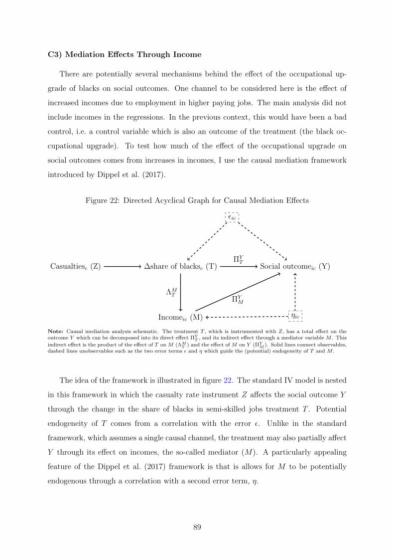
C3) Mediation Effects Through Income

There are potentially several mechanisms behind the effect of the occupational up-

grade of blacks on social outcomes. One channel to be considered here is the effect of

increased incomes due to employment in higher paying jobs. The main analysis did not

include incomes in the regressions. In the previous context, this would have been a bad

control, i.e. a control variable which is also an outcome of the treatment (the black oc-

cupational upgrade). To test how much of the effect of the occupational upgrade on

social outcomes comes from increases in incomes, I use the causal mediation framework

introduced by Dippel et al. (2017).

Figure 22: Directed Acyclical Graph for Causal Mediation Effects

Casualtiesc (Z) ∆share of blacksc (T) Social outcomeic (Y)

Incomeic (M)

εic

ηic

ΠYT

ΛMT

ΠYM

Note: Causal mediation analysis schematic. The treatment T , which is instrumented with Z, has a total effect on theoutcome Y which can be decomposed into its direct effect ΠY

T , and its indirect effect through a mediator variable M . This

indirect effect is the product of the effect of T on M (ΛMT ) and the effect of M on Y (ΠY

M ). Solid lines connect observables,dashed lines unobservables such as the two error terms ε and η which guide the (potential) endogeneity of T and M .

The idea of the framework is illustrated in figure 22. The standard IV model is nested

in this framework in which the casualty rate instrument Z affects the social outcome Y

through the change in the share of blacks in semi-skilled jobs treatment T . Potential

endogeneity of T comes from a correlation with the error ε. Unlike in the standard

framework, which assumes a single causal channel, the treatment may also partially affect

Y through its effect on incomes, the so-called mediator (M). A particularly appealing

feature of the Dippel et al. (2017) framework is that is allows for M to be potentially

endogenous through a correlation with a second error term, η.

89

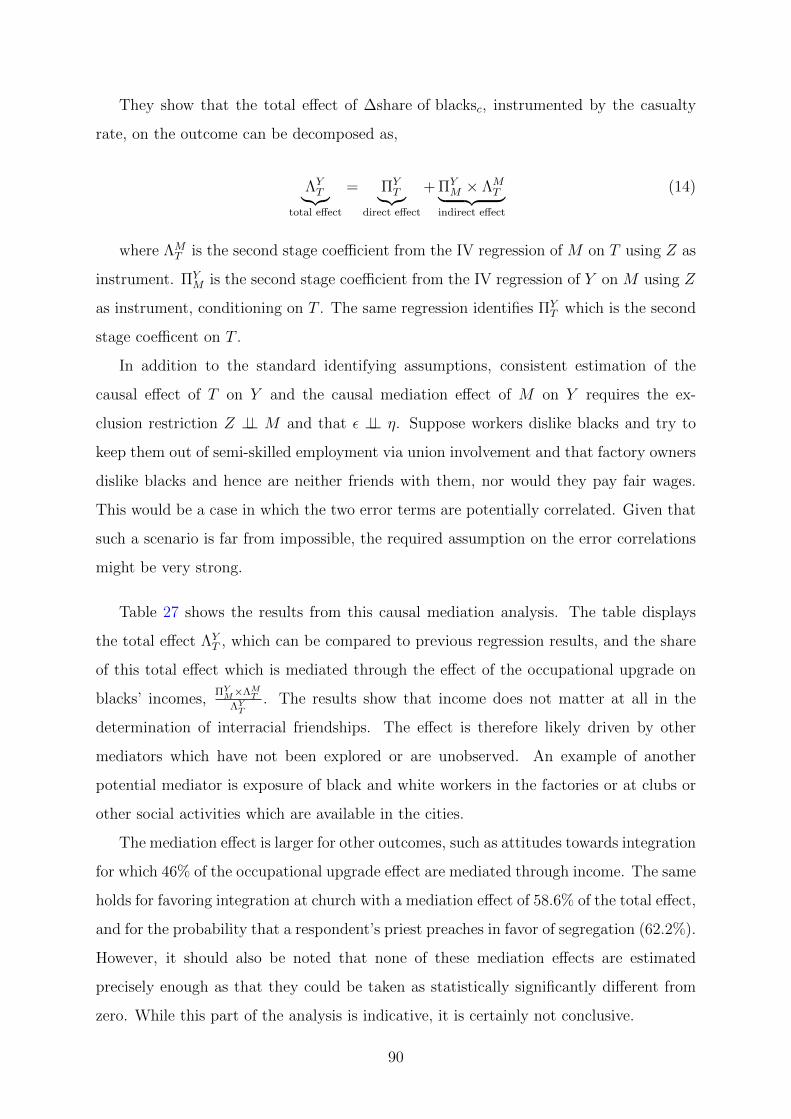
They show that the total effect of ∆share of blacksc, instrumented by the casualty

rate, on the outcome can be decomposed as,

ΛYT︸︷︷︸

total effect

= ΠYT︸︷︷︸

direct effect

+ ΠYM × ΛM

T︸ ︷︷ ︸indirect effect

(14)

where ΛMT is the second stage coefficient from the IV regression of M on T using Z as

instrument. ΠYM is the second stage coefficient from the IV regression of Y on M using Z

as instrument, conditioning on T . The same regression identifies ΠYT which is the second

stage coefficent on T .

In addition to the standard identifying assumptions, consistent estimation of the

causal effect of T on Y and the causal mediation effect of M on Y requires the ex-

clusion restriction Z ⊥⊥ M and that ε ⊥⊥ η. Suppose workers dislike blacks and try to

keep them out of semi-skilled employment via union involvement and that factory owners

dislike blacks and hence are neither friends with them, nor would they pay fair wages.

This would be a case in which the two error terms are potentially correlated. Given that

such a scenario is far from impossible, the required assumption on the error correlations

might be very strong.

Table 27 shows the results from this causal mediation analysis. The table displays

the total effect ΛYT , which can be compared to previous regression results, and the share

of this total effect which is mediated through the effect of the occupational upgrade on

blacks’ incomes,ΠY

M×ΛMT

ΛYT

. The results show that income does not matter at all in the

determination of interracial friendships. The effect is therefore likely driven by other

mediators which have not been explored or are unobserved. An example of another

potential mediator is exposure of black and white workers in the factories or at clubs or

other social activities which are available in the cities.

The mediation effect is larger for other outcomes, such as attitudes towards integration

for which 46% of the occupational upgrade effect are mediated through income. The same

holds for favoring integration at church with a mediation effect of 58.6% of the total effect,

and for the probability that a respondent’s priest preaches in favor of segregation (62.2%).

However, it should also be noted that none of these mediation effects are estimated

precisely enough as that they could be taken as statistically significantly different from

zero. While this part of the analysis is indicative, it is certainly not conclusive.

90

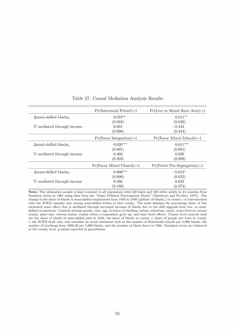
Table 27: Causal Mediation Analysis Results

Pr(Interracial Friend)=1 Pr(Live in Mixed Race Area)=1

∆semi-skilled blacksc 0.018∗∗ 0.011∗∗

(0.023) (0.029)% mediated through income 0.001 −0.442

(0.998) (0.344)

Pr(Favor Integration)=1 Pr(Favor Mixed Schools)=1

∆semi-skilled blacksc 0.020∗∗∗ 0.011∗∗∗

(0.001) (0.001)% mediated through income 0.460 0.026

(0.203) (0.909)

Pr(Favor Mixed Church)=1 Pr(Priest Pro Segregation)=1

∆semi-skilled blacksc 0.008∗∗∗ −0.013∗

(0.000) (0.052)% mediated through income 0.586 0.622

(0.186) (0.274)

Note: The estimation sample is kept constant in all regressions with 540 black and 528 white adults in 24 counties fromSouthern states in 1961 using data from the “Negro Political Participation Study” (Matthews and Prothro, 1975). Thechange in the share of blacks in semi-skilled employment from 1940 to 1950 (∆share of blacksc) in county c is instrumentedwith the WWII casualty rate among semi-skilled whites in that county. The table displays the percentage share of thisestimated main effect that is mediated through increased incomes of blacks due to the skill upgrade from low- to semi-skilled occupations. Controls include gender, race, age, location of dwelling (urban, suburban, rural), years lived in currentcounty, place size, veteran status, county where a respondent grew up, and state fixed effects. County level controls usedare the share of blacks in semi-skilled jobs in 1940, the share of blacks in county c, share of people not born in countyc, the WWII draft rate, and variables on racial sentiment such as the number of Rosenwald schools per 1,000 blacks, thenumber of lynchings from 1900-30 per 1,000 blacks, and the number of black slaves in 1860. Standard errors are clusteredat the county level, p-values reported in parentheses.

91

Data Appendix

Merging Enlistment and Casualty Records

Merging the 8.3 million observations from the WWII Army enlistment records with the

casualty records based on the Army serial number matches 78% of all casualties. These

are observations which found a unique match across both data sets. For robustness I

computed the soundex string distance of first- and surname and kept those matches for

which it was sufficiently small in order to be sure that the match was correct. Less than

one percent of these initial matches were returned to the pool of unmatched observations

because of significant differences in the names that indicated a clear mismatch despite a

perfect match on the serial number. The match rate is not perfect because of mistakes in

the serial number made by the Optical Character Recognition (OCR) software on part

of the casualty tables for which the scans are of less than ideal quality.

The remaining casualties were matched via the probabilistic string matching algo-

rithms provided by Wasi and Flaaen (2015). A one-to-one match was used to link each

casualty with a potential enlistment record based on name and serial number stratified

by state of residence. Names are matched via a tokenization and serial numbers via a

bigram algorithm. The match with the highest combined matching score was kept. This

results in a final match rate of 94%. From a random sample of 1,000 matches the error

rate was 0.6% as judged by correctness of the name, serial number, and residence. The

OCR quality of the remaining 6% of casualty observations was too poor in order to clearly

identify whether a given match was correct. These cases were dropped.

Sources of the U.S. Census County Data, 1920-1970

The main data source are the county aggregates of the U.S. Decennial Census of

Population and Housing from 1940 to 1970 and the 100% full count micro data of the

Census. For the years 1940 to 1970, the Census publishes occupational counts at the

county level where Southern states report them separated for black and white workers.

For instance, see table 23a on page 278 of the 1940 Census for Georgia shown in figure 23

which are the raw data from which I digitized the employment information at the county

level for blacks by county and skill group. Occupations are defined according to the har-

92

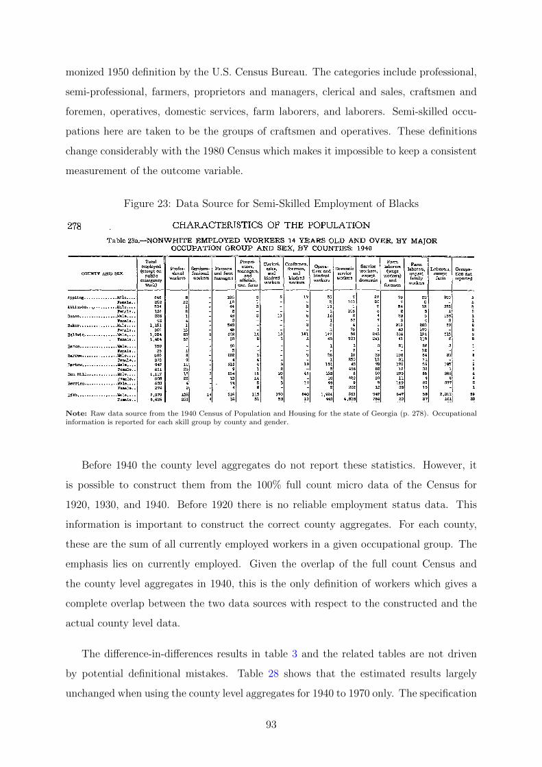
monized 1950 definition by the U.S. Census Bureau. The categories include professional,

semi-professional, farmers, proprietors and managers, clerical and sales, craftsmen and

foremen, operatives, domestic services, farm laborers, and laborers. Semi-skilled occu-

pations here are taken to be the groups of craftsmen and operatives. These definitions

change considerably with the 1980 Census which makes it impossible to keep a consistent

measurement of the outcome variable.

Figure 23: Data Source for Semi-Skilled Employment of Blacks

Note: Raw data source from the 1940 Census of Population and Housing for the state of Georgia (p. 278). Occupationalinformation is reported for each skill group by county and gender.

Before 1940 the county level aggregates do not report these statistics. However, it

is possible to construct them from the 100% full count micro data of the Census for

1920, 1930, and 1940. Before 1920 there is no reliable employment status data. This

information is important to construct the correct county aggregates. For each county,

these are the sum of all currently employed workers in a given occupational group. The

emphasis lies on currently employed. Given the overlap of the full count Census and

the county level aggregates in 1940, this is the only definition of workers which gives a

complete overlap between the two data sources with respect to the constructed and the

actual county level data.

The difference-in-differences results in table 3 and the related tables are not driven

by potential definitional mistakes. Table 28 shows that the estimated results largely

unchanged when using the county level aggregates for 1940 to 1970 only. The specification

93

with covariates fixed at their 1940 levels estimates a slightly smaller effect while inclusion

of the county-specific time trends takes away more significance. This is mostly due to the

reduced size of the pre-treatment time window but the coefficient remains as before.

Table 28: County Level Difference-in-Differences Results, 1940-1970

Outcome: % blacks in semi-skilled jobs (pre-war mean = 12.433)

(1) (2) (3) (4) (5) (6)

Casualty ratec× Post-wart 0.529∗∗∗ 0.617∗∗∗ 0.343∗∗∗ 0.586∗∗∗ 0.534∗ 0.552∗∗∗

(0.117) (0.155) (0.132) (0.162) (0.285) (0.123)

Controls Yes Yes Yes Yes1940 controls × time YesFlexible state time trends YesLinear county time trends YesDoubly-robust selection YesObservations 4,985 3,626 3,684 3,626 3,626 4,655Counties 1,388 1,229 985 1,229 1,229 1,377Adj. R2 0.885 0.901 0.905 0.908 0.919 0.880Oster’s δ 0.951 1.023 0.545 1.109 0.599 0.996

Note: Difference-in-differences regressions of the county-level share of blacks in semi-skilled occupations on the WWIIcounty casualty rate among semi-skilled whites interacted with a post-war indicator. The estimation sample containsdecennial U.S. Census data on counties in Southern states from 1940 to 1970. Controls include county and decade fixedeffects, the county draft rate, average casualty rate in the neighboring counties, log WWII spending per capita, share ofblack men, share of rural population, log median family income, share of pop. with high school degree, no. of manufacturingestablishments per capita, average manufacturing firm size, log manufacturing value added per worker, share of employmentin manufacturing, share of land in agricultural production, share of acres in cotton production, share of cash tenants, averagevalue of machinery per farm, lynchings per 1,000 blacks between 1900 and 1930, no. of Rosenwald schools per 1,000 blacks,share of acres flooded by the Mississippi in 1928, no. of slaves in 1860, Republican vote share, New Deal spending percapita 1933-35 (loans, public works, AAA, FHA loans), and the unemployment rate in 1937. Time-invariant controls areinteracted with decade fixed effects. Monetary values are deflated to 2010 U.S. dollars. The doubly-robust selection methodimplements the Belloni et al. (2014) machine learning covariate selection algorithm for testing the stability of treatmenteffects with respect to the observables. Oster’s (2017) test for selection on unobservables is reported in the final row bycomputing the coefficient of proportionality δ for which the coefficient on the semi-skilled casualty rate among whites wouldequal zero. Standard errors clustered at the county level. Significance levels are denoted by * p < 0.10, ** p < 0.05, ***p < 0.01.

94

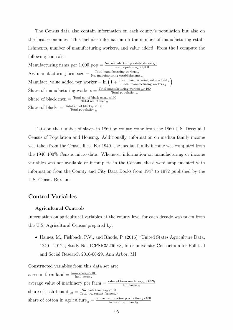
The Census data also contain information on each county’s population but also on

the local economies. This includes information on the number of manufacturing estab-

lishments, number of manufacturing workers, and value added. From the I compute the

following controls:

Manufacturing firms per 1,000 pop = No. manufacturing establishmentsctTotal populationct/1,000

Av. manufacturing firm size = Total manufacturing workersctNo. manufacturing establishmentsct

Manufact. value added per worker = ln(

1 + Total manufacturing value addedct

Total manufacturing workersct

)

Share of manufacturing workers = Total manufacturing workersct×100Total populationct

Share of black men = Total no. of black menct×100Total no. of menct

Share of blacks = Total no. of blacksct×100Total populationct

Data on the number of slaves in 1860 by county come from the 1860 U.S. Decennial

Census of Population and Housing. Additionally, information on median family income

was taken from the Census files. For 1940, the median family income was computed from

the 1940 100% Census micro data. Whenever information on manufacturing or income

variables was not available or incomplete in the Census, these were supplemented with

information from the County and City Data Books from 1947 to 1972 published by the

U.S. Census Bureau.

Control Variables

Agricultural Controls

Information on agricultural variables at the county level for each decade was taken from

the U.S. Agricultural Census prepared by:

• Haines, M., Fishback, P.V., and Rhode, P. (2016) “United States Agriculture Data,

1840 - 2012”, Study No. ICPSR35206-v3, Inter-university Consortium for Political

and Social Research 2016-06-29, Ann Arbor, MI

Constructed variables from this data set are:

acres in farm land = farm acresct×100land acresct

average value of machinery per farm = value of farm machineryct×CPItNo. farmsct

share of cash tenantsct = No. cash tenantsct×100Total no. tenant farmersct

share of cotton in agriculturect = No. acres in cotton productionct×100Acres in farm landct

95

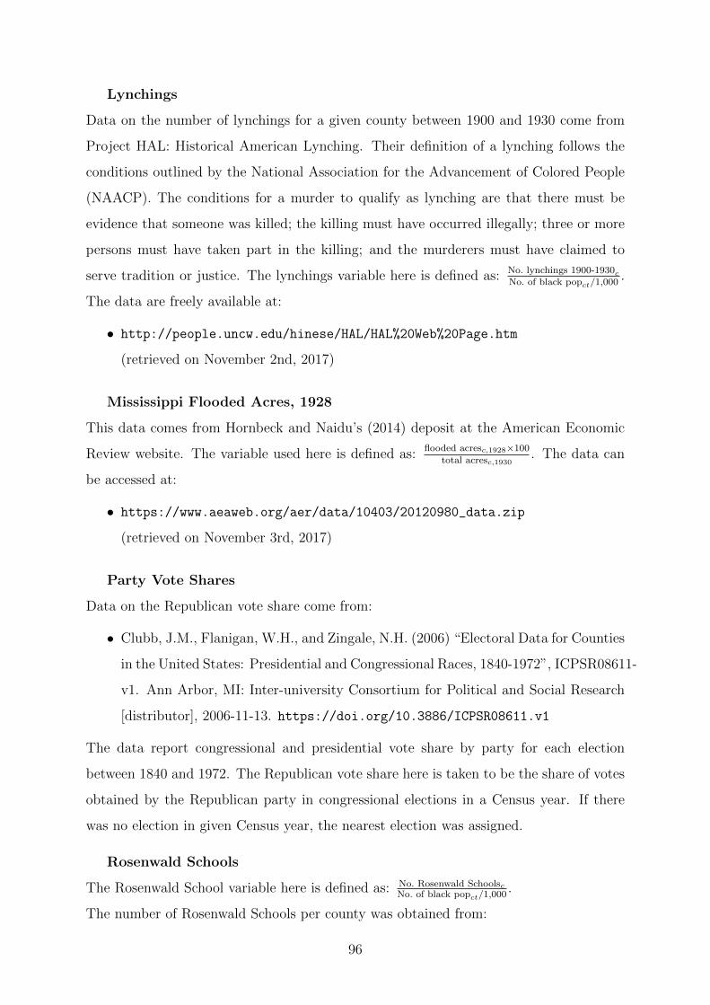
Lynchings

Data on the number of lynchings for a given county between 1900 and 1930 come from

Project HAL: Historical American Lynching. Their definition of a lynching follows the

conditions outlined by the National Association for the Advancement of Colored People

(NAACP). The conditions for a murder to qualify as lynching are that there must be

evidence that someone was killed; the killing must have occurred illegally; three or more

persons must have taken part in the killing; and the murderers must have claimed to

serve tradition or justice. The lynchings variable here is defined as: No. lynchings 1900-1930cNo. of black popct/1,000

.

The data are freely available at:

• http://people.uncw.edu/hinese/HAL/HAL%20Web%20Page.htm

(retrieved on November 2nd, 2017)

Mississippi Flooded Acres, 1928

This data comes from Hornbeck and Naidu’s (2014) deposit at the American Economic

Review website. The variable used here is defined as: flooded acresc,1928×100

total acresc,1930. The data can

be accessed at:

• https://www.aeaweb.org/aer/data/10403/20120980_data.zip

(retrieved on November 3rd, 2017)

Party Vote Shares

Data on the Republican vote share come from:

• Clubb, J.M., Flanigan, W.H., and Zingale, N.H. (2006) “Electoral Data for Counties

in the United States: Presidential and Congressional Races, 1840-1972”, ICPSR08611-

v1. Ann Arbor, MI: Inter-university Consortium for Political and Social Research

[distributor], 2006-11-13. https://doi.org/10.3886/ICPSR08611.v1

The data report congressional and presidential vote share by party for each election

between 1840 and 1972. The Republican vote share here is taken to be the share of votes

obtained by the Republican party in congressional elections in a Census year. If there

was no election in given Census year, the nearest election was assigned.

Rosenwald Schools

The Rosenwald School variable here is defined as: No. Rosenwald SchoolscNo. of black popct/1,000

.

The number of Rosenwald Schools per county was obtained from:

96

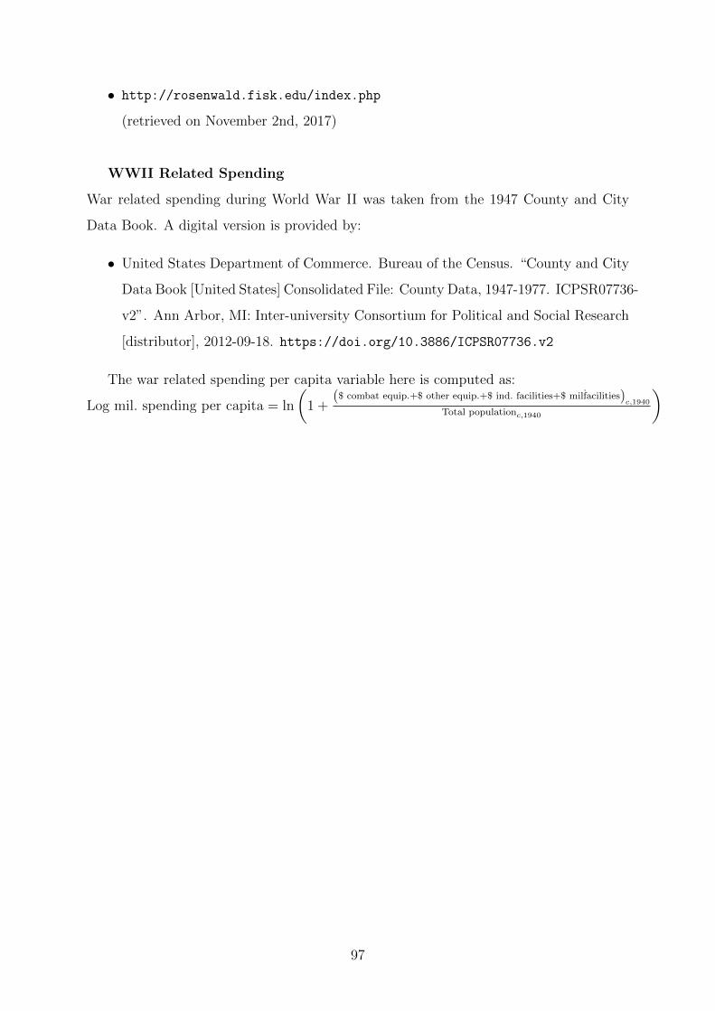
• http://rosenwald.fisk.edu/index.php

(retrieved on November 2nd, 2017)

WWII Related Spending

War related spending during World War II was taken from the 1947 County and City

Data Book. A digital version is provided by:

• United States Department of Commerce. Bureau of the Census. “County and City

Data Book [United States] Consolidated File: County Data, 1947-1977. ICPSR07736-

v2”. Ann Arbor, MI: Inter-university Consortium for Political and Social Research

[distributor], 2012-09-18. https://doi.org/10.3886/ICPSR07736.v2

The war related spending per capita variable here is computed as:

Log mil. spending per capita = ln

(1 +

($ combat equip.+$ other equip.+$ ind. facilities+$ milfacilities)c,1940

Total populationc,1940

)

97