WORLD ME T E O ROL O GICAL O RGANIZAT I O N … · world me t e o rol o gical o rganizat i o n...

WORLD ME T E O ROL O GICAL O RGANIZAT I O N

INSTRUMENTS AND OBSERVING METHODS R E P O R T No. 79

OPERATIONAL ASPECTS OF WIND PROFILER RADARS

by

J. Dibbern, Germany D. Engelbart, Germany U. Goersdorf, Germany

N. Latham, United Kingdom V. Lehmann, Germany

J. Nash, United Kingdom T. Oakley, United Kingdom

H. Richner, Switzerland H. Steinhagen, Germany

WMO/TD No. 1196 2003

2

NOTE

The designations employed and the presentation of material in this publication do not imply the expression of any opinion whatsoever on the part of the Secretariat of the World Meteorological

Organization concerning the legal status of any country, territory, city or area, or its authorities, or concerning the limitation of the frontiers or boundaries.

This report has been produced without editorial revision by the Secretariat. It is not an official

WMO publication and its distribution in this form does not imply endorsement by the Organization of the ideas expressed.

FOREWORD In recent years we have been witnessing an increased use of wind profiler radars. At present there are more than 150 wind profiler radars operated worldwide by NHMSs, universities, research institutes, environmental agencies, and airport authorities. Considering that the development of operational wind profiler radars are evolving rapidly and that standardization and the improvement of quality control procedures is vital to wide operational acceptance of this system, the Commission for Instruments and Methods of Observation agreed that its work in the field of wind profilers be continued with the aim to provide advise to members on their operational aspects. Different operational networks exist around the world. For example, the NOAA Profiler Network (NPN), which had been operating since 1992, currently has 32 profiler sites in the continental United States operating at 404 MHz and three sites in Alaska operating at 449 MHz. NOAA-FSL (Forecast Systems Laboratory) had started a project in cooperation with about 30 other agencies owning profilers to acquire boundary layer profiler wind and temperature data from about 65 profilers which would be collected by the Profiler Control Center and processed into hourly, quality-controlled products, and distributed. In Japan the Japan Meteorological Agency (JMA) had completed an operational network of twenty-five 1.3 GHz wind profilers in 2001. The profilers were installed throughout the Japanese islands with a control center at Tokyo, where after quality control of the data, the Doppler velocities obtained every 10 minutes at each site were translated into wind vectors. The JMA was also planning further improvement of the spatial resolution of the profiler network by increasing the number of systems to 31. In Europe, networking of wind profiler radars had been co-ordinated by the COST-76 project, a co-operation between NMHSs', research institutes, universities and industry. Sixteen systems send data operationally to the UK Met Office which, in collaboration with European partners, had developed an infrastructure for network operations and real time Internet display. After COST-76 concluded in 2000, the Council of the European Meteorological Services Network (EUMETNET) agreed in October 2001 to establish the wind profiler programme WINPROF to enable continuation of the operational network. This Instrument and Methods of Observation (IOM) Report is dedicated to the development of VHF/UHF wind profilers for use in European observing systems. In preparation is an IOM Report on operational use of wind profilers in USA and Japan. This is expected to be published in mid 2004. I would like to thank all those who provided information from their networks and the CIMO Surface Measurements Working Group, especially Mr J. Dibbern from Dewtcher Wetterdienst.

(Dr. R.P. Canterford)

Acting President of the Commission for

Instruments and Methods of Observation

i

Content

1. Status of frequency allocations for wind profiler radar............................................................................... 1 1.1. Introduction......................................................................................................................................... 1 1.2. ITU Resolution COM5-5 (WRC-97) .................................................................................................. 2

1.2.1. Original Text ............................................................................................................................... 2 1.2.2. Notes ........................................................................................................................................... 5

1.3. Excerpt from the frequency tables of the ITU Radio Regulations with the footnotes referring directly to wind profiler radars..................................................................................................................................... 6 1.4. Parameters for characterising the electromagnetic properties of wind profilers ................................. 9

1.4.1. Introduction ................................................................................................................................. 9 1.4.2. Measurements at the transmitter output .................................................................................... 10

1.4.2.1. Bandwidth ............................................................................................................................. 10 1.4.2.2. Harmonics ............................................................................................................................. 10 1.4.2.3. Subharmonics........................................................................................................................ 10 1.4.2.4. Spurious emissions................................................................................................................ 10 1.4.2.5. Power .................................................................................................................................... 10

1.4.3. Measurements of the emitted signal .......................................................................................... 11 1.4.4. Field strength around the antenna ............................................................................................. 11

APPENDIX I: Definitions according to ITU Radio Regulations...................................................................... 12 APPENDIX II: Notes related to the determination of the various parameters.................................................. 13 2. Performance (availability, accuracy)......................................................................................................... 14

2.1. Height coverage ................................................................................................................................ 14 2.1.1. Wind.......................................................................................................................................... 14

2.2.1.1. Theory ................................................................................................................................... 14 2.2.1.2. Results................................................................................................................................... 16

2.1.2. Virtual temperature ................................................................................................................... 20 2.1.2.1. Theory ................................................................................................................................... 20 2.1.2.2. Results................................................................................................................................... 20

2.2. Accuracy ........................................................................................................................................... 21 2.2.1. About the definition of measuring error.................................................................................... 21 2.2.2. Estimation of accuracy .............................................................................................................. 23

2.2.2.1. Comparisons of wind profiles between wind profiler and rawinsondes................................ 24 2.2.2.2. Comparisons of temperature profiles between RASS and radiosondes ................................ 30 2.2.2.3. Comparisons with model data (NWP)................................................................................... 31

2.2.3. Error sources for wind measurements ....................................................................................... 36 2.2.3.1. Unwanted backscattering processes ...................................................................................... 36 2.2.3.2. Internal and external Radio Frequency Interference (RFI).................................................... 38 2.2.3.3. Inhomogeneity of the 3D windfield ...................................................................................... 39 2.2.3.4. Interpretation error ................................................................................................................ 39 2.2.3.5. Unsuitable parameter adjustments......................................................................................... 40 2.2.3.6. Hardware faults ..................................................................................................................... 42

2.2.4. Error sources for temperature measurements ............................................................................ 42 2.3. Reliability.......................................................................................................................................... 43

3. Quality evaluation ..................................................................................................................................... 44 3.1. Introduction....................................................................................................................................... 44 3.2. Data availability ................................................................................................................................ 45 3.3. Identification of anomalous measurements ....................................................................................... 45 3.4. Quality evaluation techniques ........................................................................................................... 48

3.4.1. Comparisons with numerical forecast fields ............................................................................. 48 3.4.2. Comparison with Fields Generated By Integrated Observing Systems..................................... 49 3.4.3. Random errors from the consistency of time series of measurements ...................................... 51

3.5. Random error results from CWINDE-99 .......................................................................................... 54 3.6. Summary ........................................................................................................................................... 57

4. Maintenance .............................................................................................................................................. 58 4.1. Introduction....................................................................................................................................... 58 4.2. Requirements for maintenance.......................................................................................................... 58 4.3. Remote monitoring and diagnosis of WPR/RASS............................................................................ 59 4.4. Routine Maintenance ........................................................................................................................ 60

ii

4.5. Preventive Maintenance .................................................................................................................... 62 4.6. Expenses............................................................................................................................................ 66

5. Operational characteristics ........................................................................................................................ 67 5.1. Characteristics of an operational system ........................................................................................... 67 5.2. An example of remote operation of wind profilers ........................................................................... 68

6. Siting considerations ................................................................................................................................. 71 7. Data coding ............................................................................................................................................... 73

7.1. Introduction....................................................................................................................................... 73 7.2. Background ....................................................................................................................................... 74 7.3. Some remarks to the general structure of BUFR............................................................................... 74 7.4. Motivation of choices........................................................................................................................ 76 7.5. Conclusions....................................................................................................................................... 83

8. Networking................................................................................................................................................ 84 8.1. Input .................................................................................................................................................. 85 8.2. Real-time processing......................................................................................................................... 87 8.3. Output................................................................................................................................................ 88

9. Economic aspects of wind profiler radar................................................................................................... 90 9.1. 50 MHz systems................................................................................................................................ 91 9.2. 400 MHz systems.............................................................................................................................. 91 9.3. 1 GHz systems................................................................................................................................... 92

1

This report is a collection of output from COST 76 Working Groups on topics associated with wind profiler operations. In several cases, a section is based on the work of one country. This reflects the division of tasks within the working groups, and the national reports represent the experience or views of those who were developing operational procedures in the given area. These views can be expected to evolve with time as more experience is gained with various systems.

Section 5.1 contains a report on the status of frequency allocations for profilers. When planning to operate a wind profiler it is essential to understand national limitations on the frequencies to be used. As wind profilers have been given secondary status, operations have to co-exist with other higher priority radiofrequency services. The limitations on frequency use may also vary with location within a given country, as well as from country to country in Europe. It will always be necessary to negotiate use through the national radiocommunication authorities.

Section 5.2 indicates the data availability and accuracy of wind measurements that can be expected from the present generation of wind profilers, based on performance surveys conducted by Lindenberg observatory. It also identifies the reasons for large wind measurement anomalies that have been noted on some occasions. Section 5.3 describes the techniques used in real-time quality evaluation, based on procedures developed by the CWINDE network hub in the UK.

Section 5.4 is a consideration of wind profiler maintenance policies, based on the development work at Lindenberg Observatory.

Section 5.5 provides information on the operational characteristics of present wind profilers based on experience from a pilot network of four wind profilers in the UK.

Section 5.6 is a summary of some of the problems that have been identified in selecting sites for the present profilers in Europe.

Section 5.7 is a summary of the results of a major block of work performed by the two main working groups to generate suitable codes for circulating wind profiler data on the meteorological telecommunications network. This is followed by a report from the UK of the methods used to circulate wind profiler data in the CWINDE network in Section 5.8.

Section 5.9 provides information on the economic factors influencing the operational costs of wind profiler use. This information is based on several thorough surveys of national experience covering all the participants within COST 76.

1. Status of frequency allocations for wind profiler radar

1.1. Introduction

At the World Radio Conference 1997 (WRC-97), the Plenary accepted Resolution COM5-5 as well as Footnotes S5.162A and S5.291A. This finally allows the meteorological community to operate wind profiler radars operationally and enables them to make full use of the potential of this unique instrument.

The adoption of the Resolution and the footnotes marked the end of significant efforts over a period of no less than ten years. Activities on many levels - national and international -- were necessary to find suitable and acceptable operating frequencies for wind profilers. Numerous individuals as well as many international organisations helped to reach this long awaited

2

decision. The essence of the ITU decisions is summarised in the next two sections, in addition, a few explanatory notes are given.

Finally, a document is reprinted which is the result of joint activities of COST-76 and national frequency allocation authorities. It lists the recommended parameters which should be determined for wind profiler radars; they allow comparisons of characteristics and enable allocations more easily. The document includes also the most important ITU definitions of widely used parameters. Some of these are defined differently for engineering purposes, a fact that has led to many misunderstandings and heated debates.

1.2. ITU Resolution COM5-5 (WRC-97)

The Resolution reproduced here is the full, original text adopted in the Final Acts of the World Radiocommunication Conference 1997. At the end (Section 5.1.2.2), some comments are added, these should allow decisions for practical applications, point out some pitfalls and help to better understand the decisions. Please note that ITU text is in frames.

1.2.1. Original Text

RESOLUTION COM5-5 (WRC-97)

IMPLEMENTATION OF WIND PROFILER RADARS

The World Radiocommunication Conference (Geneva, 1997),

3

having noted a request to ITU from the Secretary-General of the World Meteorological Organisation (WMO), in May 1989, for advice and assistance in the identification of appropriate frequencies near 50 MHz, 400 MHz and 1000 MHz in order to accommodate allocations and assignments for wind profiler radars, considering a) that wind profiler radars are vertically-directed Doppler radars exhibiting characteristics similar to radiolocation systems; b) that wind profiler radars are important meteorological systems used to measure wind direction and speed as a function of altitude; c) that it is necessary to use frequencies in different ranges in order to have options for different performance and technical characteristics; d) that, in order to conduct measurements up to a height of 30 km, it is necessary to allocate frequency bands for these radars in the general vicinity of 50 MHz (3 to 30 km), 400 MHz (500 m to about 10 km) and 1000 MHz (100 m to 3 km); e) that some administrations have either already deployed, or plan to expand their use of, wind profiler radars in operational networks for studies of the atmosphere and to support weather monitoring, forecasting and warning programs; f) that the ITU radiocommunication study groups have studied the technical and sharing considerations between wind profiler radars and other services allocated in bands near 50 MHz, 400 MHz and 1000 MHz, considering further a) that some administrations have addressed this matter nationally by assigning frequencies for use by wind profiler radars in existing radiolocation bands or on a non-interference basis in other bands; b) the work of the Voluntary Group of Experts on the Allocation and Improved Use of the Radio Frequency Spectrum and Simplification of the Radio Regulations supports increased flexibility in the allocation of frequency spectrum, noting in particular a) that wind profiler radars operating in the meteorological aids service in the band 400.15 - 406.0 MHz interfere with satellite emergency position-indicating radio beacons operating in the mobile-satellite service in the band 406.0 - 406.1 MHz under No. S5.266; b) that in accordance with No. S5.267, any emission capable of causing harmful interference to the authorised uses of the band 406 - 406.1 MHz is prohibited,

4

resolves 1 to urge administrations to implement wind profiler radars as radiolocation service systems in the following bands, having due regard to the potential for incompatibility with other services and assignments to stations in these services, thereby taking due account of the principle of geographical separation, in particular with regard to neighbouring countries, and keeping in mind the category of service of each of these services: 46 - 68 MHz in accordance with No. S5.162A 440 - 450 MHz 470 - 494 MHz in accordance with No. S5.291A 904 - 928 MHz in Region 2 only 1270 - 1295 MHz 1300 - 1375 MHz; 2 that, in case compatibility between wind profiler radars and other radio applications operating in the band 440 - 450 MHz or 470 - 494 MHz cannot be achieved, the bands 420 - 435 MHz or 438 - 440 MHz could be considered for use; 3 to urge administrations to implement wind profiler radars in accordance with Recommendations ITU-R M. 1226, ITU-R M. 1085-1 and ITU-R M. 1227 for the frequency bands around 50 MHz, 400 MHz and 1000 MHz, respectively; 4 to urge administrations not to implement wind profiler radars in the band 400.15 - 406 MHz; and 5 to urge administrations currently operating wind profiler radars in the band 400.15 - 406.0 MHz to discontinue them as soon as possible, instructs the Secretary-General to bring this Resolution to the attention of ICAO (International Civil Aviation Organisation), IMO and WMO.

5

1.2.2. Notes

Resolution COM5-5 basically states that for the 50 MHz wind profiler radars case-by-case allocations be made. 400 MHz systems could be operated between 440 and 450 MHz in North-America and between 470 and 494 MHz in Europe. For 1 GHz systems, finally, 915 MHz is the first choice in North-America, the range 1270 to 1295 MHz in Europe and 1300 to 1375 MHz in Japan. However, there are quite a few additional possibilities allowing for deviations from this principle in cases when national practice precludes its application.

An excerpt of the ITU Frequency Tables is given in Section 3 below; for details -- in particular for footnotes not referring directly to wind profiler radars -- please consult the Radio Regulations.

ad "noting in particular": The problem addressed here is the possible interference between wind profiler radars and the COSPAR/SARSAT system.

ad "resolves 1":

46 - 68 MHz: Here, case-by-case allocations will have to be made on a non-interference basis.

440 - 450 MHz: This band is allocated world-wide to FIXED and MOBILE (except aeronautical mobile) on the primary and to Radiolocation on the secondary level. However, particularly in European countries, frequencies in this band have been allocated to sensitive, in some cases even safety-of-life services. Hence, in most European countries, wind profiler radars cannot be operated in this band. In Canada and in the United States this seems to be the preferred band for 400 MHz systems.

470 - 494 MHz: A number of European countries (see S5.291) intend to allocate frequencies in this range to wind profiler radars; for them, this band is the workable alternative to 440 - 450 MHz. The range 470 - 494 MHz encompasses channels 21, 22, and 23 of the television band IV/V. Note that the use of channel 21 is generally discouraged; in fact, some countries use it as guard band between television and sensitive services just below 470 MHz.

904 - 928 MHz: This band (center frequency 915 MHz) is designated for industrial, scientific and medical (ISM) applications in Region 2 (basically the Americas). In this area, 1 GHz wind profiler radars can be operated here.

1270 - 1295 MHz: In Regions 1 and 3 where the ISM band is not available, or in Region 2 where operation in the ISM band is not feasible, this radiolocation band is available for wind profiler radar operations.

1300 - 1375 MHz: Where neither in the ISM band nor in the radiolocation band operation is feasible, this band may be used for wind profiler radar operations.

ad "resolves 2": As mentioned above, in most European countries wind profiler radars cannot be operated in the 440 - 450 MHz band. In some countries it may also be difficult to use the broadcast band 470 - 494 MHz. This "resolves" is an open option to use the radiolocation band between 420 - 440 MHz in Europe. However, the band 435 - 438 MHz is not available for wind profiler radar operations because this range is used world-wide by the amateur-satellite service. Note also that the Radio Regulations list numerous footnotes defining special national uses of the 420 - 440 MHz range.

6

1.3. Excerpt from the frequency tables of the ITU Radio Regulations with the footnotes referring directly to wind profiler radars

• Text in frames is original wording from ITU Radio Regulations, text out of the frames are comments and additions.

• Please note the conventions in the ITU RR Frequency Tables: Services typed in CAPITALS are allocated on a PRIMARY basis, Services in Upper-and-Lower-Case are allocated on a secondary basis.

• In this excerpt of the ITU Frequency Tables, only those footnotes are listed that are relevant for operating wind profiler radar.

• Table elements particularly relevant for the operation of wind profiler radars are shaded.

Region 1 Region 2 Region 3

44 - 47 FIXED

MOBILE

S5.162A

47 - 50

FIXED

MOBILE

47 – 50

FIXED

MOBILE

BROADCASTING

50 – 54 AMATEUR

47 - 68

BROADCASTING

S5.162A

54 - 68

BROADCASTING

Fixed

Mobile

54 – 68

FIXED

MOBILE

BROADCASTING

S5.162A Additional allocation: in Germany, Austria, Belgium, Bosnia and Herzegovina, China, Vatican, Denmark, Spain, Estonia, Finland, France, Ireland, Iceland Italy, Latvia, The Former Yugoslav Republic of

7

Note: Originally, it was proposed to allocate frequencies to wind profiler radars only on the band 47 - 68 MHz, this range coinciding with the existing segmentation. However, because one European country operates already a wind profiler radar just below that segment, the band was extended downwards to 46 MHz.

Macedonia, Liechtenstein, Lithuania, Luxembourg, Moldova, Monaco,Norway, Netherlands, Poland, Portugal, Slovakia, the Czech Republic,the United Kingdom, Russia, Sweden, Switzerland and Turkey, theband 46 - 68 MHz is also allocated to the radiolocation service on a secondary basis. This use is limited to the operation of wind profilerradars in accordance with Resolution COM5-5 (WRC-97).


420 - 430 FIXED

MOBILE

Radiolocation

430 - 440

AMATEUR

RADIOLOCATION

430 – 440

RADIOLOCATION

Amateur

440 - 450 FIXED

MOBILE except aeronautical mobile

Radiolocation


470 - 790 BROADCASTING

S5.291A

470 - 512

BROADCASTING

Fixed

Mobile

470 -585

FIXED

MOBILE

BROADCASTING

S5.291A Additional allocation: in Germany, Austria, Denmark, Estonia, Finland, Liechtenstein, Norway, Netherlands, the Czech Republic and Switzerland, the band 470 - 494 MHz is also allocated to the radiolocation service on a secondary basis. This use is limited to the operation of wind profiler radars in accordance with Resolution COM5-5 (WRC-97).

8

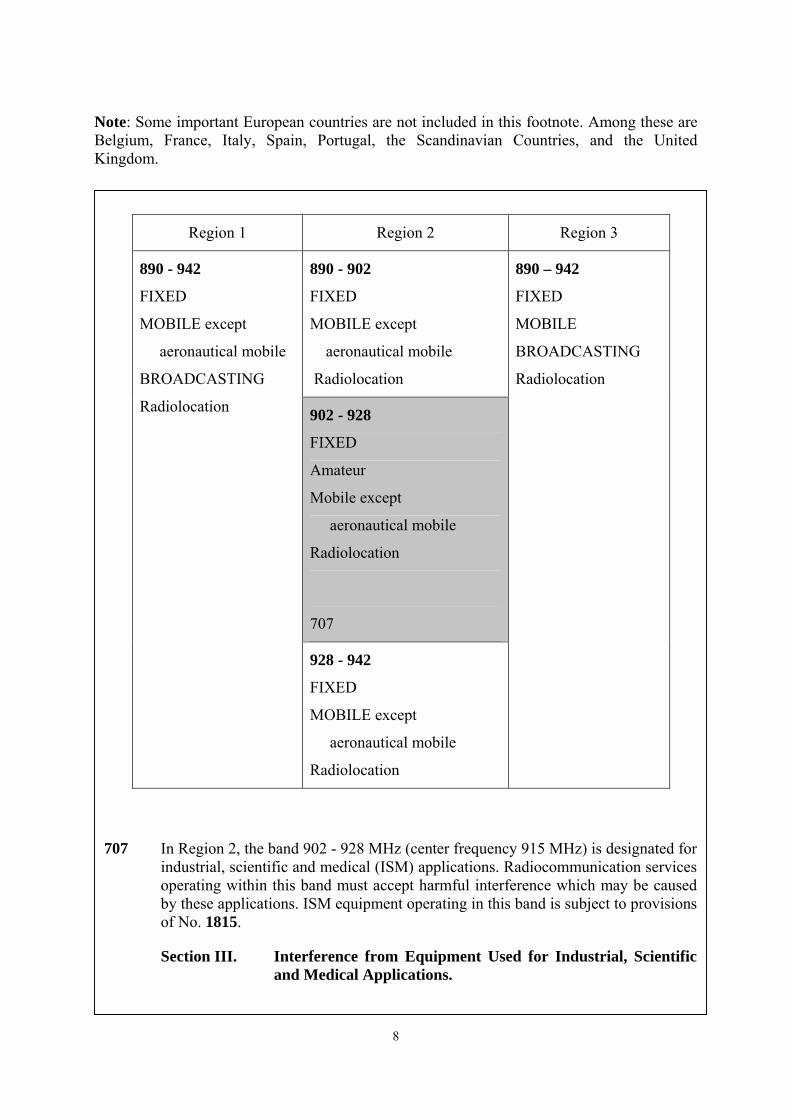
Note: Some important European countries are not included in this footnote. Among these are Belgium, France, Italy, Spain, Portugal, the Scandinavian Countries, and the United Kingdom.


890 - 902

FIXED

MOBILE except

aeronautical mobile

Radiolocation

902 - 928

FIXED

Amateur

Mobile except

aeronautical mobile

Radiolocation

707

890 - 942

FIXED

MOBILE except

aeronautical mobile

BROADCASTING

Radiolocation

928 - 942

FIXED

MOBILE except

aeronautical mobile

Radiolocation

890 – 942

FIXED

MOBILE

BROADCASTING

Radiolocation

707 In Region 2, the band 902 - 928 MHz (center frequency 915 MHz) is designated for industrial, scientific and medical (ISM) applications. Radiocommunication services operating within this band must accept harmful interference which may be caused by these applications. ISM equipment operating in this band is subject to provisions of No. 1815.

Section III. Interference from Equipment Used for Industrial, Scientific and Medical Applications.

9

1.4. Parameters for characterising the electromagnetic properties of wind profilers

1.4.1. Introduction

For all investigations about the electromagnetic compatibility of wind profilers, the following parameters should be measured in addition to whatever other parameters are required by national or local authorities. Having a set of identically measured parameters allows a direct comparison of quantities obtained for different instruments in different locations; if these are not available, the quantities have to be computed with assumption which are not always well founded.

All parameters should be determined for all pulse lengths available for the particular profiler. If the number of pulse lengths is greater than four, the parameters should at least be determined for the longest and shortest pulse length plus two additional ones.

If pulse coding is available, the spectra should be determined for emissions with and without pulse coding (only for those pulse lengths for which coding is intended to be used).

Terms which are marked with * are further defined in the Appendix "Definitions".

1815 §10. Administrations shall take all practical and necessary steps to ensure that radiation from equipment used for industrial, scientific and medical applications is minimal and that, outside the bands designated for use by this equipment, radiation from such equipment is at a level that does not cause harmful interference to a radiocommunication service and, in particular, to a radionavigation or any other safety service operating in accordance with the provisions of these Regulations.


1260 - 1300 RADIOLOCATION

EARTH EXPLORATION SATELLITE (active)

SPACE RESEARCH (active)

Amateur

1300 - 1350 AERONAUTICAL RADIONAVIGATION

Radiolocation

1350 - 1400

FIXED

MOBILE

RADIOLOCATION

1350 – 1400

RADIOLOCATION

10

1.4.2. Measurements at the transmitter output

1.4.2.1. Bandwidth

- plot the spectrum with a resolution bandwidth of at least 300 kHz (i.e. with a resolution band width ≤ 300 kHz)

- determine the frequency at which there is maximum signal

- determine the pulse peak power in the spectrum (preferably with a resolution bandwidth of 100 kHz)

- determine the necessary bandwidth*

= necessary bandwidth: Distance on the frequency axis between the two nulls on each side of the main peak at the nominal frequency

- determine the occupied bandwidth*

= occupied bandwidth: whenever possible proceed according to Radio Regulation and integrate the spectrum. If this effort cannot be made, determine the distance between the points on either side of the main peak at which the power has decreased by 23 dB below the power of the main peak

- compute ratio of occupied to necessary bandwidth

- determine the effective pulse width from the spectrum

= take the frequency difference between the secondary and tertiary spectral peak. Its reciprocal value is the effective pulse width.

1.4.2.2. Harmonics

- plot the spectrum centred at twice the nominal frequency, i.e., at the second harmonic

- determine the power level of the second harmonic with respect to that at the nominal frequency.

1.4.2.3. Subharmonics

- plot the spectrum centred at half the nominal frequency, i.e., at the subharmonic

- determine the power level of the subharmonic with respect to that at the nominal frequency.

1.4.2.4. Spurious emissions

- using an appropriate attenuator, reduce the power at the main frequency and plot the spectrum over a frequency range as wide as possible

- from this spectrum, determine the level of spurious emissions* in absolute values (i.e. mW).

1.4.2.5. Power

- plot power versus time (i.e., take a sweep)

- determine the pulse repetition frequency from the time difference between the individual power peaks

11

- determine the average emitted power (see Note 1, when measuring the emitted signal also Note 2, Appendix II)

- determine the duty cycle (see Note 3, Appendix II).

1.4.3. Measurements of the emitted signal

All the above-mentioned parameters can be determined directly at the output of the transmitter. In order to obtain information on the performance and the filtering effect of the antenna, all power and bandwidth measurements should be repeated for radiated signals, using an appropriate receiving antenna. (If measurements in the main beam at a known distance from the profiler antenna can be achieved, also the antenna system gain can be determined.)

1.4.4. Field strength around the antenna

Determine field strength in the far-field of the antenna, at the nominal frequency, in different directions and at different distances from the antenna 10 m above the surface. If the antenna is polarised, measure in the horizontal as well as in the vertical polarisation plane.

These values must be determined for a height of 10 m above ground. Measurements should be made directly at this height because height correction computations are not reliable, the use of computational height corrections is strongly discouraged.

Preferably, field strength values should be presented in graphical form (i.e., as a map showing isolines).

12

APPENDIX I: Definitions according to ITU Radio Regulations

Necessary bandwidth: For a given class of emission, the width of the frequency band which is just sufficient to ensure the transmission of information at the rate and with the quality required under specified conditions.

(Radio Regulations Chapter 1, Section VI "Characteristics of emissions and radio equipment", Paragraph 146)

Occupied bandwidth: The width of a frequency band such that, below the lower and above the upper frequency limits, the mean powers emitted are each equal to a specified percentage β/2 of the total mean power of a given emission.

Unless otherwise specified by the CCIR (Comité Consultatif International des Radiocommunications) for the appropriate class of emission, the value for β/2 should be taken as 0.5 %.


Out-of-band emission (en français: emission hors bande): Emission on a frequency or frequencies immediately outside the necessary bandwidth which results from the modulation process, but excluding spurious emissions.


Spurious emission (en français: rayonnement non essentiel): Emission on a frequency or frequencies which are outside the necessary bandwidth and the level of which may be reduced without affecting the corresponding transmission of information. Spurious emissions include harmonic emissions, parasitic emissions, intermodulation products and frequency conversion products, but exclude out-of-band emissions.


Unwanted emissions (en français: rayonnements non désirés): Consist of spurious emissions and out-of-band emissions.


13

APPENDIX II: Notes related to the determination of the various parameters

Note 1:

In order to obtain the pulse peak power Ppeak from the measurements, the pulse attenuation factor a must be taken into account:

Ppeak = P'peak - a

where a = 20 log(1.5 · t · RBW)

with [Ppeak] = [a] = dB P'peak: measured power in dB t: pulse length in sec RBW: resolution bandwidth in Hz

Note 2:

The effective radiated power Perp is determined from field strength measurements using the equation

Perp = 249

2

.)dE( ⋅

with [Perp] = W E: fieldstrength in V/m d: distance in m

Note 3:

The duty cycle DC is most easily determined as

DC = 100 · (PRF · t)

with [DC] = % PRF: pulse repetition frequency in Hz t: pulse length in sec

14

2. Performance (availability, accuracy)

2.1. Height coverage

The vertical range and temporal availability of wind and temperature measurements are an important criterion for an operational use of wind profiler/RASS. Especially, the maximum range depends not only from technical properties of the system but also from the meteorological conditions. Therefore, the maximum range shows significant temporal variations. The maximum range is determined by the strength of the backscattered power and its ratio to the noise. The dependence of the backscattered power on the atmospheric properties is described by the radar equation. Gathering all system parameters in the constant α, the radar equation can be written in the following simple form:

22)(lr

PrP To

ηα= (5.2.1.1)

where PT is the transmitting power, η is the volume reflectivity, r is the range and l is a attenuation parameter. It is obviously that the backscattered power is proportional to the transmitting power PT and the volume reflectivity η as well as inverse proportional to the square of range and the attenuation parameter. Furthermore, the detectability of the signal depends on the strength of noise.

For given system parameters variations in the availability, especially in the maximum range, are caused by variations of volume reflectivity and/or the attenuation of the electromagnetic and acoustic waves in the atmosphere.

The relative availability corresponding Equation (5.2.1.2) was calculated in order to evaluate the performance of the different wind profiler/RASS systems.

100xvaluespossibleofnumber

valuesvalidofnumber%intyavailabililativeRe = (5.2.1.2)

2.1.1. Wind

2.2.1.1. Theory

As mentioned above the maximum range depends on the system parameters and the volume reflectivity. The attenuation of electromagnetic waves is proportional to the frequency. For frequencies used for wind profiler radars (50 - 1290 MHz), the attenuation is several scales smaller than other effects and therefore, it can be neglected.

More important is the volume reflectivity. If the characteristic length of backscattering structures are within the inertial subrange the volume reflectivity is given by the following equation (Tatarskii, 1961):

η = 0.38 cn2 λ1/3 (5.2.1.1.1.1)

cn

2 is the structure parameter of the refractive index, which can be described by an equation from Ottersten (1969):

15

cn

2 = a (∆n2)L0-2/3 (5.2.1.1.1.2)

where a is a constant, ∆n is the mean variance of the refractive index and L0 is the outer scale of turbulence. In order to get an impression of the distribution of cn

2 in the atmosphere both the refractive index as well as the strength of turbulence must be known. To get reliable information about turbulence in the free atmosphere is difficult, but it is possible to calculate the gradient of the refractive index from radiosoundings. The refractive index can be calculated by an equation given by Bean and Dutton (1966):

1)1073,36,77(10 256 ++= −

Te

TPn (p in hPa; e in hP) (5.2.1.1.1.3)

In the troposphere both temperature and water vapour have the largest effect on variations of n, whereas in the stratosphere only the temperature is relevant for n variations. Figure 5.2.1.1.1.1 shows mean profiles of the refractive index gradient calculated on the base of a one-year radiosoundings at Lindenberg. Notable is a secondary minimum at about 9 km, which can also be recognised by a lower availability of 482 MHz wind measurements (see 5.2.1.1.2).

Figure 5.2.1.1.1.1: Mean profiles of refractive index gradient, calculated on the base of radiosounding during one year.

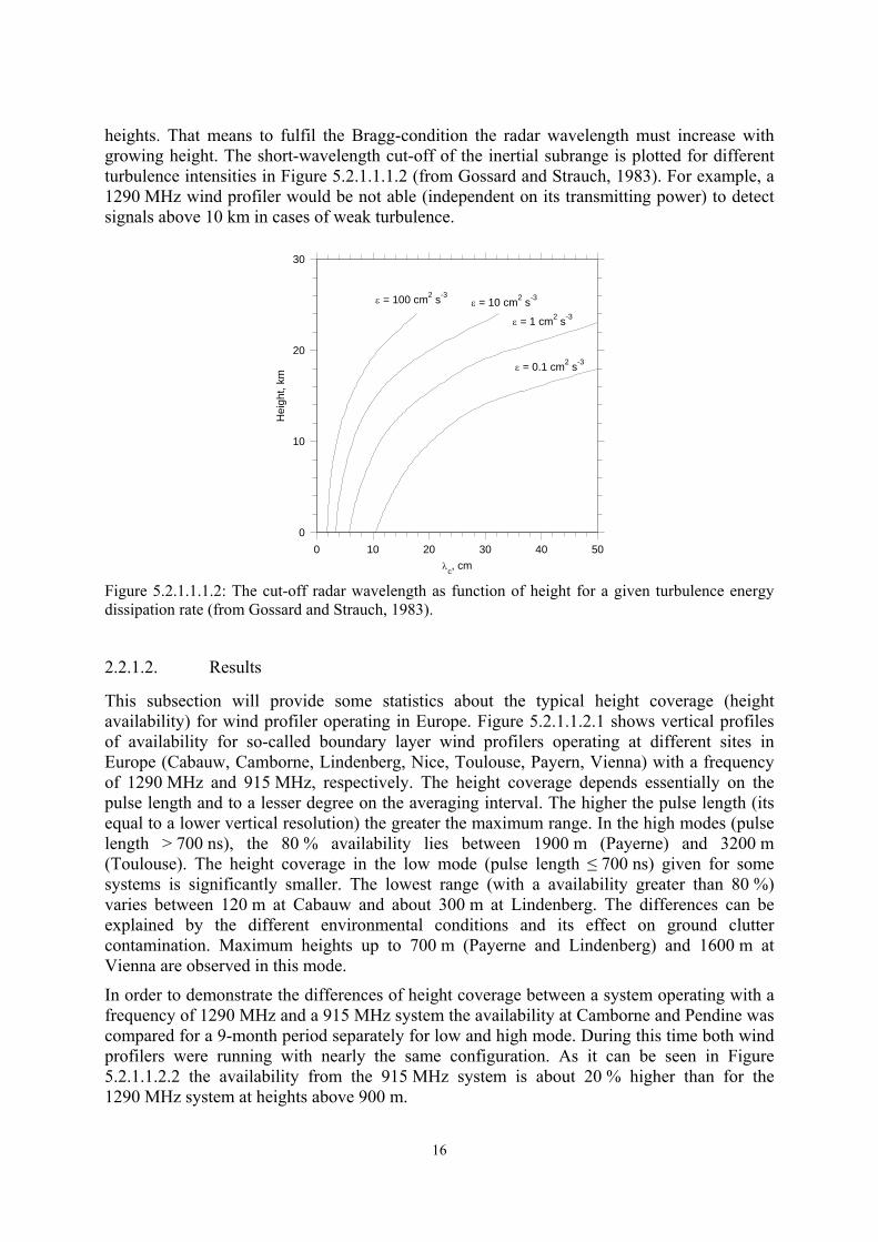
Furthermore, the maximum detectable range depends on the radar frequency or wavelength, respectively, because the inner scale of the inertial subrange is growing with increasing

0

5000

10000

15000

20000

0.00001 0.0001 0.001 0.01

WinterSpringSummerAutumn

(∂(n-1)x106/∂z)2, m-2

Hei

ght,

m

16

heights. That means to fulfil the Bragg-condition the radar wavelength must increase with growing height. The short-wavelength cut-off of the inertial subrange is plotted for different turbulence intensities in Figure 5.2.1.1.1.2 (from Gossard and Strauch, 1983). For example, a 1290 MHz wind profiler would be not able (independent on its transmitting power) to detect signals above 10 km in cases of weak turbulence.

0

10

20

30

0 10 20 30 40 50

ε = 0.1 cm2 s-3

ε = 1 cm2 s-3

ε = 10 cm2 s-3 ε = 100 cm2 s-3

λc, cm

Hei

ght,

km

Figure 5.2.1.1.1.2: The cut-off radar wavelength as function of height for a given turbulence energy dissipation rate (from Gossard and Strauch, 1983).

2.2.1.2. Results

This subsection will provide some statistics about the typical height coverage (height availability) for wind profiler operating in Europe. Figure 5.2.1.1.2.1 shows vertical profiles of availability for so-called boundary layer wind profilers operating at different sites in Europe (Cabauw, Camborne, Lindenberg, Nice, Toulouse, Payern, Vienna) with a frequency of 1290 MHz and 915 MHz, respectively. The height coverage depends essentially on the pulse length and to a lesser degree on the averaging interval. The higher the pulse length (its equal to a lower vertical resolution) the greater the maximum range. In the high modes (pulse length > 700 ns), the 80 % availability lies between 1900 m (Payerne) and 3200 m (Toulouse). The height coverage in the low mode (pulse length ≤ 700 ns) given for some systems is significantly smaller. The lowest range (with a availability greater than 80 %) varies between 120 m at Cabauw and about 300 m at Lindenberg. The differences can be explained by the different environmental conditions and its effect on ground clutter contamination. Maximum heights up to 700 m (Payerne and Lindenberg) and 1600 m at Vienna are observed in this mode.

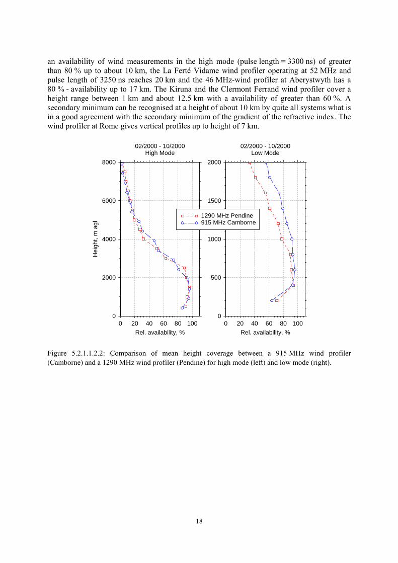
In order to demonstrate the differences of height coverage between a system operating with a frequency of 1290 MHz and a 915 MHz system the availability at Camborne and Pendine was compared for a 9-month period separately for low and high mode. During this time both wind profilers were running with nearly the same configuration. As it can be seen in Figure 5.2.1.1.2.2 the availability from the 915 MHz system is about 20 % higher than for the 1290 MHz system at heights above 900 m.

17

Figure 5.2.1.1.2.1: Vertical profiles of mean availability for the wind measurements of 1290 MHz and 915 MHz wind profilers at different sites in Europe.

Wind profiler systems operating at lower frequencies are able to measure the wind throughout the whole troposphere and partly over the lowest part of the stratosphere. The height range depends of course on the antenna aperture product (e.g. transmitting power) and the parameter configuration (e.g. pulse lengthcycle, duty cycle). The 482 MHz system at Lindenberg yields

0

2000

4000

6000

8000

10000

0 20 40 60 80 100

700 ns2800 ns

Rel availability, %

Hei

ght,

m a

glCabauw (290 MHz)

Jan.1998 - Dec. 1998

0 20 40 60 80 100

700 ns2800 ns

Rel availability, %

Lindenberg (1290 MHz)Nov.1993 - Oct.1996

0

2000

4000

6000

8000

10000

0 20 40 60 80 100

1400 ns

Rel availability, %

Hei

ght,

m a

gl

Nice (1290 MHz) Apr. 2000 - Oct. 2000

0 20 40 60 80 100

950 ns

Rel availability, %

Toulouse (1274 MHz) Oct. 1999 - Apr. 2000

0 20 40 60 80 100

700 ns2800 ns

Rel availability, %

Payerne (1290 MHz)Jan.1998 - Dec. 1998

0 20 40 60 80 100

300 ns

Rel availability, %

Vienna (1290 MHz) Nov. 1999 - Oct. 2000

0 20 40 60 80 100

700 ns2800 ns

Rel availability, %

Camborne (915 MHz) Feb. 2000 - Oct. 2000

18

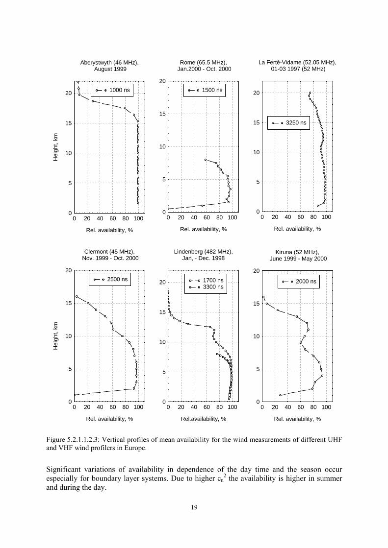
an availability of wind measurements in the high mode (pulse length = 3300 ns) of greater than 80 % up to about 10 km, the La Ferté Vidame wind profiler operating at 52 MHz and pulse length of 3250 ns reaches 20 km and the 46 MHz-wind profiler at Aberystwyth has a 80 % - availability up to 17 km. The Kiruna and the Clermont Ferrand wind profiler cover a height range between 1 km and about 12.5 km with a availability of greater than 60 %. A secondary minimum can be recognised at a height of about 10 km by quite all systems what is in a good agreement with the secondary minimum of the gradient of the refractive index. The wind profiler at Rome gives vertical profiles up to height of 7 km.

0

500

1000

1500

2000

0 20 40 60 80 100Rel. availability, %

02/2000 - 10/2000Low Mode

0

2000

4000

6000

8000

0 20 40 60 80 100

1290 MHz Pendine915 MHz Camborne

Rel. availability, %

Hei

ght,

m a

gl

02/2000 - 10/2000High Mode

Figure 5.2.1.1.2.2: Comparison of mean height coverage between a 915 MHz wind profiler (Camborne) and a 1290 MHz wind profiler (Pendine) for high mode (left) and low mode (right).

19

0

5

10

15

20

0 20 40 60 80 100

1000 ns


Hei

ght,

kmAberystwyth (46 MHz),

August 1999

0

5

10

15

20

0 20 40 60 80 100

1500 ns


Rome (65.5 MHz), Jan.2000 - Oct. 2000

0

5

10

15

20

0 20 40 60 80 100

3250 ns


La Fertè-Vidame (52.05 MHz), 01-03 1997 (52 MHz)

0

5

10

15

20

0 20 40 60 80 100

1700 ns3300 ns

Rel.availability, %

Lindenberg (482 MHz),Jan, - Dec. 1998

0

5

10

15

20

0 20 40 60 80 100

2000 ns


Kiruna (52 MHz), June 1999 - May 2000

0

5

10

15

20

0 20 40 60 80 100

2500 ns


Hei

ght,

km

Clermont (45 MHz), Nov. 1999 - Oct. 2000

Figure 5.2.1.1.2.3: Vertical profiles of mean availability for the wind measurements of different UHF and VHF wind profilers in Europe.

Significant variations of availability in dependence of the day time and the season occur especially for boundary layer systems. Due to higher cn

2 the availability is higher in summer and during the day.

20

2.1.2. Virtual temperature

2.1.2.1. Theory

The vertical range of a RASS depends essentially on the transmitted electromagnetic and acoustic power as well as on parameters describing the acoustic attenuation (Lataitis, 1992; Bauer-Pfundstein, 1998). Three different types of attenuation can be separated:

• classical absorption due to inner friction, heat conduction and heat radiation • molecular absorption due to relaxation processes • excess attenuation due to the broadening of the acoustic beam

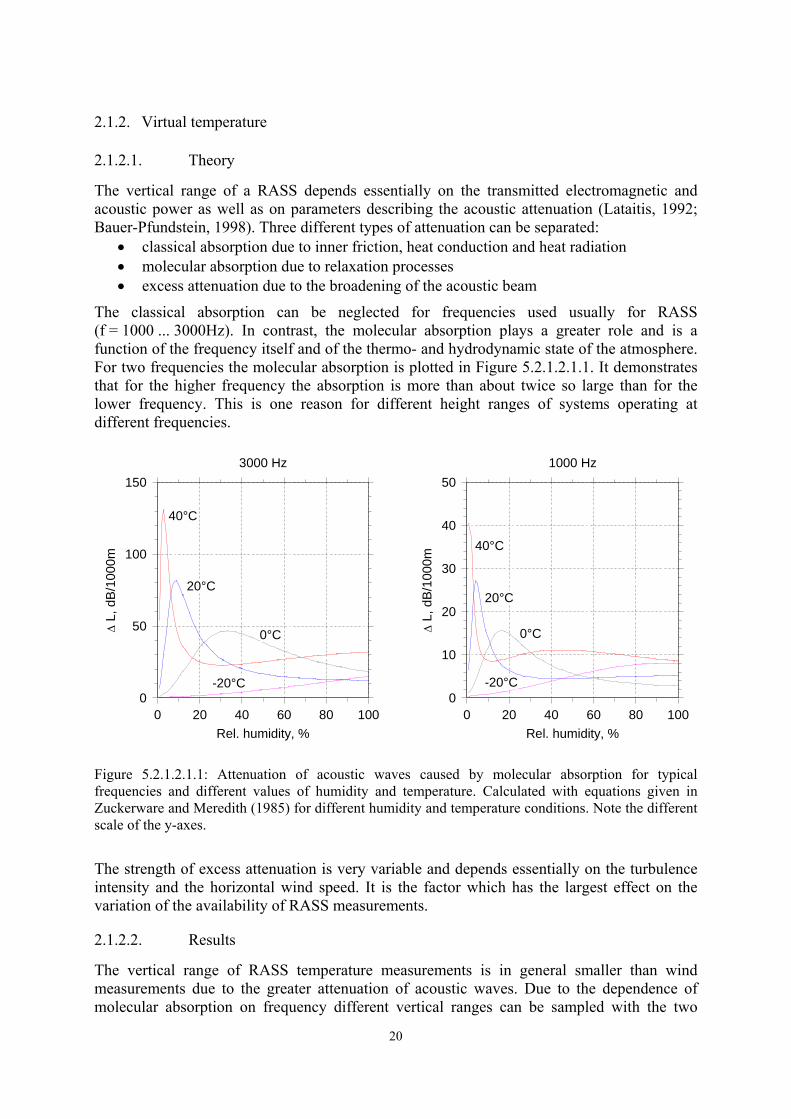
The classical absorption can be neglected for frequencies used usually for RASS (f = 1000 ... 3000Hz). In contrast, the molecular absorption plays a greater role and is a function of the frequency itself and of the thermo- and hydrodynamic state of the atmosphere. For two frequencies the molecular absorption is plotted in Figure 5.2.1.2.1.1. It demonstrates that for the higher frequency the absorption is more than about twice so large than for the lower frequency. This is one reason for different height ranges of systems operating at different frequencies.

0

50

100

150

0 20 40 60 80 100

-20°C

0°C

20°C

40°C

Rel. humidity, %

∆ L

, dB/

1000

m

3000 Hz

0

10

20

30

40

50

0 20 40 60 80 100

-20°C

0°C

20°C

40°C

Rel. humidity, %

∆ L

, dB/

1000

m

1000 Hz

Figure 5.2.1.2.1.1: Attenuation of acoustic waves caused by molecular absorption for typical frequencies and different values of humidity and temperature. Calculated with equations given in Zuckerware and Meredith (1985) for different humidity and temperature conditions. Note the different scale of the y-axes.

The strength of excess attenuation is very variable and depends essentially on the turbulence intensity and the horizontal wind speed. It is the factor which has the largest effect on the variation of the availability of RASS measurements.

2.1.2.2. Results

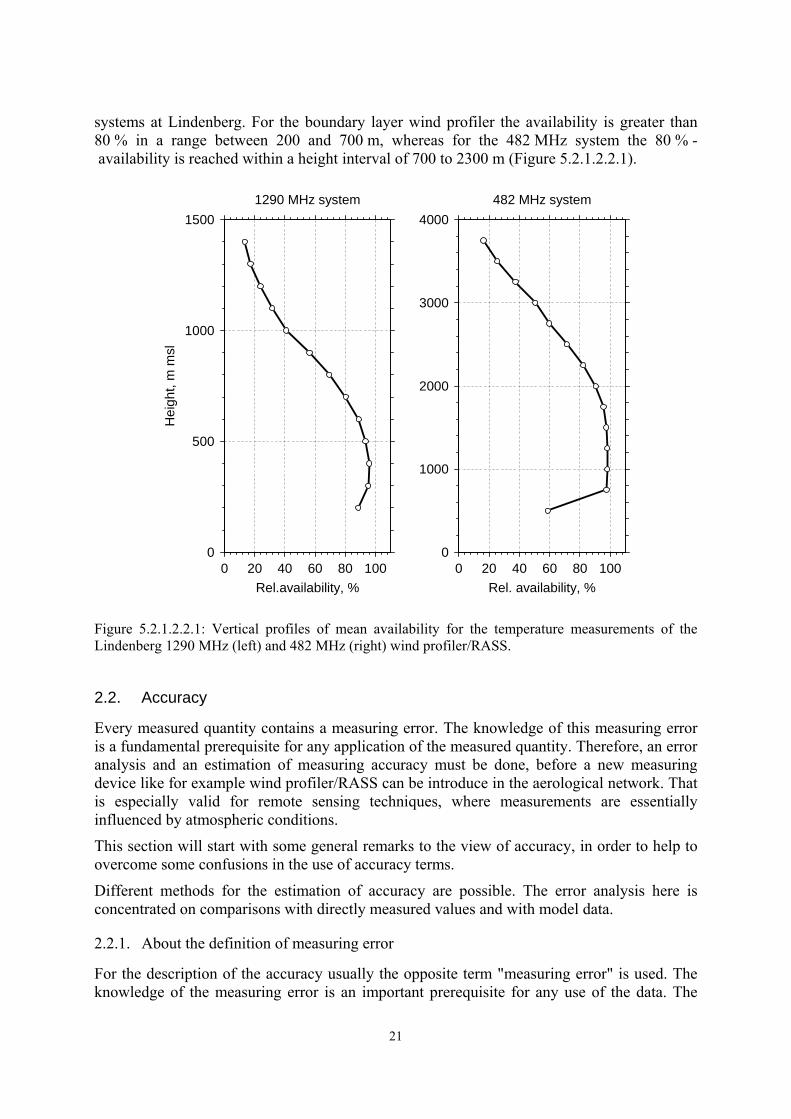
The vertical range of RASS temperature measurements is in general smaller than wind measurements due to the greater attenuation of acoustic waves. Due to the dependence of molecular absorption on frequency different vertical ranges can be sampled with the two

21

systems at Lindenberg. For the boundary layer wind profiler the availability is greater than 80 % in a range between 200 and 700 m, whereas for the 482 MHz system the 80 % - availability is reached within a height interval of 700 to 2300 m (Figure 5.2.1.2.2.1).

0

1000

2000

3000

4000

0 20 40 60 80 100Rel. availability, %

482 MHz system

0

500

1000

1500

0 20 40 60 80 100Rel.availability, %

Hei

ght,

m m

sl

1290 MHz system

Figure 5.2.1.2.2.1: Vertical profiles of mean availability for the temperature measurements of the Lindenberg 1290 MHz (left) and 482 MHz (right) wind profiler/RASS.

2.2. Accuracy

Every measured quantity contains a measuring error. The knowledge of this measuring error is a fundamental prerequisite for any application of the measured quantity. Therefore, an error analysis and an estimation of measuring accuracy must be done, before a new measuring device like for example wind profiler/RASS can be introduce in the aerological network. That is especially valid for remote sensing techniques, where measurements are essentially influenced by atmospheric conditions.

This section will start with some general remarks to the view of accuracy, in order to help to overcome some confusions in the use of accuracy terms.

Different methods for the estimation of accuracy are possible. The error analysis here is concentrated on comparisons with directly measured values and with model data.

2.2.1. About the definition of measuring error

For the description of the accuracy usually the opposite term "measuring error" is used. The knowledge of the measuring error is an important prerequisite for any use of the data. The

22

measurement error xerr is the deviation of the value xm measured with any system to the "true" value xt. xxx tmerr

−= (5.2.2.1.1) The "true" value is a limit value, which can be approached but not reached. Therefore, it is necessary to estimate the "true" value either by theoretical considerations or by (reference-) measuring systems with known accuracy.

xtrue xmeasured

S.D.S.D.

Bias

P(x)

Figure 5.2.2.1.1: Definition of bias (equivalent to accuracy) and standard deviation (equivalent to precision) on the base of the distribution (probability distribution function) of individual measurements.

For the error analysis and for the development of corrections it is useful to separate the measurement error in following parts on the base of its statistical behaviour:

! systematic error Systematic errors are deviations from the "true" value in a preferred direction. Such errors are potential detectable and correctable. Averaging individual measurements does not reduce the systematic error.

! random error Random errors are deviations without preferred direction (stochastic deviations). The random error of an individual measurement cannot be eliminated. Therefore, this error part determines the precision of a measurement. Averaging individual measurements improve the precision.

! large (gross) errors Large errors are characterised by systematic or random deviations from the "true" value larger than a given threshold. Large systematic errors are usually caused by general problems in the function of the system. Large random errors occur sporadically caused by internal or external disturbances. Due to its large deviation to the "true" value large random errors can be eliminated by quality control algorithm in most cases.

Each error part can be described by the equations given in Table 5.2.2.1.1 on the base of a reference value, whereas Figure 5.2.2.1.1 illustrates the meaning of the individual error parts on the base of individual measurements. The table includes also some other terms used often

23

in the literature. In this section we want use the terms bias and standard deviation (S.D.) to describe the systematic and the random errors. The total error of wind profiler/RASS measurements shall be characterised here by the term accuracy.

It should be noted, that the error parts have a different relevance in dependence on the use of the data . For example, the influence of a systematic error for climatology investigations is more important than a random error. On the other hand the random error plays a dominant role for the use of the data in numerical weather prediction models, whereas a systematic error can be accepted within certain limits, when all input data have a systematic error of the same magnitude. The example shows that the analysis of the different error parts is a fundamental task in the estimation of accuracy.

Error type Mathematic description Other names systematic error mean deviation:

)(11

Bi

N

ii xx

Nx −=∆ ∑

=

(5.2.2.1.1)

bias, accuracy

random error standard deviation (S.D.):

∑−

∆−−

=N

iix xx

N 1

2)(1

1σ (5.2.2.1.2)

22 )( xrmsex ∆−=σ (5.2.2.1.3)

mean square deviation, precision, statistic error, repeatability

large error xBiigi xxfore σ3>− (5.2.2.1.4) outlier

total error "root-mean-square error":

∑=

−=N

iBii xx

Nrmse

1

2)(1 (5.2.2.1.5)

Bi

N

ii xx

Nd −= ∑

=1

1 (5.2.2.1.6)

mean square error, comparability, measuring uncertainty mean absolute error

mean amount of difference vector )(1 2

1

2 vuN

mavdN

iδδ += ∑

=

(5.2.2.1.7) used only for wind vector

Table 5.2.2.1.1: Equations to calculate the different error parts with respect to a reference value.

2.2.2. Estimation of accuracy

The estimation of the accuracy of wind and temperature measurements can be performed with different methods which are: • Evaluation of accuracy using error propagation • Comparisons with other systems (like rawinsondes, tower) • Comparisons with model data • Using redundant information (Ito, 1997; Strauch et al., 1987) • Using selfconsistency of measurements (Nash and Lyth, 1997; Nash et al., 2000).

24

Each of these methods has advantages and disadvantages. But only comparisons with other collocated systems like rawinsondes, aircraft or tower instrumentations provide direct information about the systematic and the random error (bias and standard deviation, respectively). Comparisons with numerical model fields (analyses and short term forecasts) can also provide information about both types of errors, as long as the fields have been influenced by a suitable number of reliable measurements around the location considered and the magnitude of the short term forecast errors are known The other methods are suitable to estimate the random error without the use of other systems. Therefore, these methods can be used for routine quality evaluation (see Section 5.3).

2.2.2.1. Comparisons of wind profiles between wind profiler and rawinsondes

Although the differences between wind profiler radars and in-situ measurements are a combination of the measurement errors of both systems and the atmospheric variability associated with the horizontal and temporal separation of the measurements, such comparisons are the only method to estimate possible systematic deviations. Furthermore, rawinsondes are the current standard system in the aerological network, against that each new system should be evaluated. These comparisons between wind profiler and rawinsondes have always played an important role in the evaluation of quality and accuracy of wind profiler measurements (Weber and Wuertz, 1990; Astin and Thomas, 1991; Riddle et al., 1996; May, 1993; Steinhagen et al., 1994).

Comprehensive comparisons (> 1000) have been carried out at Lindenberg because rawinsondes are launched four times a day on the same place as the wind profiler site. At Lindenberg, Vaisala radiosondes are used for PTU measurements and a tracking radar serves for wind measurements. Due to these long term comparisons an evaluation of accuracy is possible for all times of the day and all seasons under different meteorological conditions. Figures 5.2.2.2.1.1 and 5.2.2.2.1.2 show vertical profiles of the bias and the standard deviation for wind speed and wind direction for both wind profilers (482 MHz and 1290 MHz) operating at Lindenberg. Table 5.2.2.2.1.1 contains a corresponding summary of the most important statistical parameters.

25

0

4000

8000

12000

16000

1.0 1.5 2.0 2.5S.D., m/s

0

4000

8000

12000

16000

-1.0 -0.5 0 0.5 1.0Bias, m/s

Hei

ght,

m m

sl

0

4000

8000

12000

16000

-10 -5 0 5 10Bias, °

Hei

ght,

m m

sl

0

4000

8000

12000

16000

0 10 20 30S.D., °

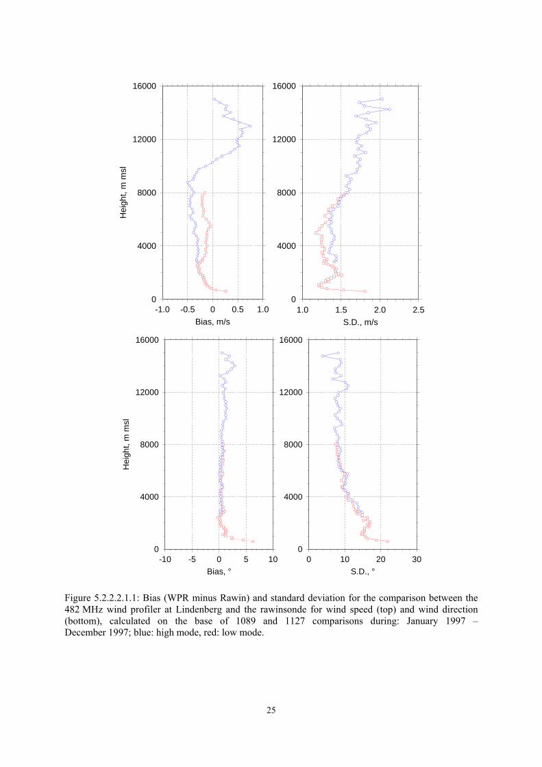
Figure 5.2.2.2.1.1: Bias (WPR minus Rawin) and standard deviation for the comparison between the 482 MHz wind profiler at Lindenberg and the rawinsonde for wind speed (top) and wind direction (bottom), calculated on the base of 1089 and 1127 comparisons during: January 1997 � December 1997; blue: high mode, red: low mode.

26

0

4000

8000

12000

16000

1.0 1.5 2.0 2.5S.D., m/s

0

4000

8000

12000

16000

-1.0 -0.5 0 0.5 1.0Bias, m/s

Hei

ght,

m m

sl

0

2000

4000

6000

-10 0 10Bias, °

Hei

ght,

m m

sl

0

2000

4000

6000

0 10 20 30 40S.D., °

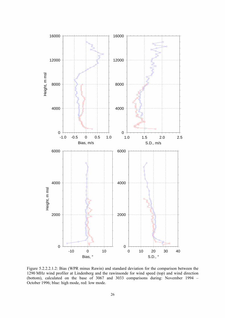
Figure 5.2.2.2.1.2: Bias (WPR minus Rawin) and standard deviation for the comparison between the 1290 MHz wind profiler at Lindenberg and the rawinsonde for wind speed (top) and wind direction (bottom), calculated on the base of 3067 and 3033 comparisons during: November 1994 � October 1996; blue: high mode, red: low mode.

27

The wind speed bias of the 482 MHz wind profiler (TWP), especially in the high mode, varies depends on altitude. There was a negative maximum at about 9000 m with -0.5 m.s-1. At heights above 10 km the bias changes sign and reaches a positive maximum at about 13 km. In the low mode the bias is smaller than 0.3 m.s-1 over the whole range. The systematic height dependent error can be explained by a range error, because a correlation between the deviation and the gradient of wind speed exists (Figure 5.2.2.2.1.3). The reasons for such a range error are either a non-uniform vertical profile of radar reflectivity or an inaccurate system delay or both (Muschinski et al., 1999). Assuming, the assigned height for the TWP-profile would be reduced by a constant amount of 170 m, the bias would be smaller than 0.25 m.s-1 in the troposphere and 0.5 m.s-1 in the stratosphere.

LAP-HighM v d

LAP-LowM v d

TWP-HighM v d

TWP-LowM v d

Period Number of Comparisons Bias, m.s-1/° S.D., m.s-1/° MBDV, m.s-1/°

Nov.1993-Oct.1996 3067

0.07 -1.22 1.501 19.46

2.09

Nov.1993-Oct.19963033

0.35 0.91 1.529 20.96

2.19

Jan.1997-Dec.1997 1089

-0.11 0.64 1.566 9.44

2.07

Jan.1997-Dec.19971127

-0.16 0.89 1.349 12.96

1.75 Gauß-Fit Bias, m.s-1/° S.D., m.s-1/°

0.09 -0.92 1.221 6.96

0.48 0.95 1.231 7.51

-0.27 -0.06 1.289 4.52

-0.16 0.06 1.125 5.88

Table 5.2.2.2.1.1: Statistics for the comparison: wind profiler - rawinsonde at Lindenberg for the 482 MHz system (TWP) and the 1290 MHz system (LAP) (v: wind speed; d: wind direction).

5000

10000

15000

10 15 20 25

482 MHz wind profilerRawin

Mean wind speed, m/s

Hei

ght,

m m

sl

Figure 5.2.2.2.1.3: Mean profiles of horizontal wind speed, calculated on the base of rawinsoundings and measurements of the 482 MHz wind profiler (high mode) at Lindenberg for January 1997 to December 1997.

28

The standard deviation of wind speed varies for both modes between 1.2 m.s-1 in the middle of the troposphere and about 2 m.s-1 in the stratosphere. One reason for the increasing standard deviation with height is the increasing distance between the location of the radiosonde measurement and the wind profiler measurement as the balloon moves away from the launch site. A lower S.D. is observed in the low mode, because the vertical resolution is more adapted to the rawinsonde height intervals.

The bias of wind direction is independent of the mode and smaller than 3° and the standard deviation is smaller than 15° over the whole range except at lowest range gates, where the tracking radar shows greater inaccuracies due to the manual tracking of the balloon at these heights. Comparisons between the 1290 MHz wind profiler (LAP) high mode and rawinsondes yield a bias smaller than 0.25 m.s-1 and 5°, respectively and a standard deviation in the range of 1.2 m.s-1 to 1.6 m.s-1 and 12° to 25°. The bias of the low mode wind speed is significantly greater with values up to 0.9 m.s-1. The reason for the differences in the bias of the high mode and the low mode is not known.

Rawinsonde comparisons performed at Payerne over one year yielded a significant bias in wind speed up to maximum of -0.7 m.s-1 in the high mode and ± 0.2 m.s-1 in the low mode (Figure 5.2.2.2.1.4). At heights greater than 500 m wind direction differences are smaller than 10°.

29

Figure 5.2.2.2.1.4: Bias (WPR minus Rawin, solid lines) and standard deviation (dashed lines) for the comparison between the 1290 MHz wind profiler at Payerne (high and low mode) and rawinsonde for wind speed and wind direction.

Comparisons between wind profiler/RASS measurements from the lowest range gates and tower instrumentation have been performed at Cabauw. The profiler underestimates wind speed compared to the tower sensors from -0.4 m.s-1 to up to -0.8 m.s-1. The standard deviations varied between 0.9 and 1.2 m.s-1. Further a dependence of the bias on the wind speed was analysed for the tower comparison at Cabauw which is in agreement with results at Lindenberg. An explanation for this effect does not exist yet.

Significant annual and diurnal variations of accuracy could not be observed at Lindenberg. Only 1290 MHz wind profiler measurements are disturbed by migrating birds when operating with long pulse length (see also previous subsection). For the statistic given above such measurements have been ignored.

30

Precipitation can influences the accuracy of wind measurements by different effects mentioned above. When the comparison results are separated for different kinds of precipitation the accuracy decreases with higher intensity and duration of precipitation. Therefore, the implementation of a more advanced moment estimation algorithm is an urgent task.

Figure 5.2.2.2.1.5: Mean amount of the difference vector (WPR-rawinsonde) in dependence of precipitation, calculated for November 1993 to October 1996 (1290 MHz wind profiler) and January 1997 to December 1997 (482 MHz wind profiler).

2.2.2.2. Comparisons of temperature profiles between RASS and radiosondes

Figure 5.2.2.2.2.1 shows the bias and the standard deviation of the temperature profiles measured with the 482 MHz wind profiler/RASS at Lindenberg.

1000

2000

3000

4000

-0.5 0 0.5 1.0Bias, K

Hei

ght,

m m

sl

1000

2000

3000

4000

0.4 0.6 0.8 1.0S.D., K

Figure 5.2.2.2.2.1: Bias (RASS minus radiosonde) and standard deviation between uncorrected (circle) and corrected (squares) RASS virtual temperatures and radiosonde virtual temperatures for the 482 MHz wind profiler/RASS. The triangles reveal results where the vertical velocity correction is not applied.

31

The profiles have been calculated with the routine algorithm (e.g. without any correction) and with considering corrections for vertical velocity, more accurate constants and a more precise range (Goersdorf and Lehmann, 2000). Without corrections the bias varies between 0.2 K at the lowest level, a maximum value of 0.9 K at about 1200 m and 0.6 K at upper heights. Most remarkable is the height dependence of the bias, resulting in an underestimation of the temperature gradient.

The application of the corrections reduces the bias to less than 0.3 K considering the whole height range. The standard deviation has been decreased at some levels by up to 0.3 K. For the case that the vertical velocity correction is neglected, the agreement between RASS and radiosonde temperatures will be closer than 0.2 K. This improvement can be explained by the bias in the mean vertical velocity measured with wind profiler, which seems to be a general problem (Angevine et al., 1998).

2.2.2.3. Comparisons with model data (NWP)

Comparisons with the model forecast as a nearly independent reference are a customary method to evaluate the quality and accuracy, respectively of model input data. Therefore, it was obvious to compare wind profiler data with numerical weather prediction model values, in order to answer the question if wind profiler data are suitable as model input data and if they are even more accurate than rawinsonde values. In the frame of CWINDE and COST 76 a routine monitoring has been established by Météo France and UK Met Office for all wind profiler stations providing data to the CWINDE data base. The monitoring includes a comparison of wind profiler data against the background field of the numerical models (�ARPEGE� in France, �Unified-model� in UKMO). Of course, the model wind field is strongly based on rawinsonde data, the main source for aerological data in numerical models and its errors. Therefore, differences between model and wind profiler data are not only caused by errors of wind profiler measurements, but also by model and representativeness errors.

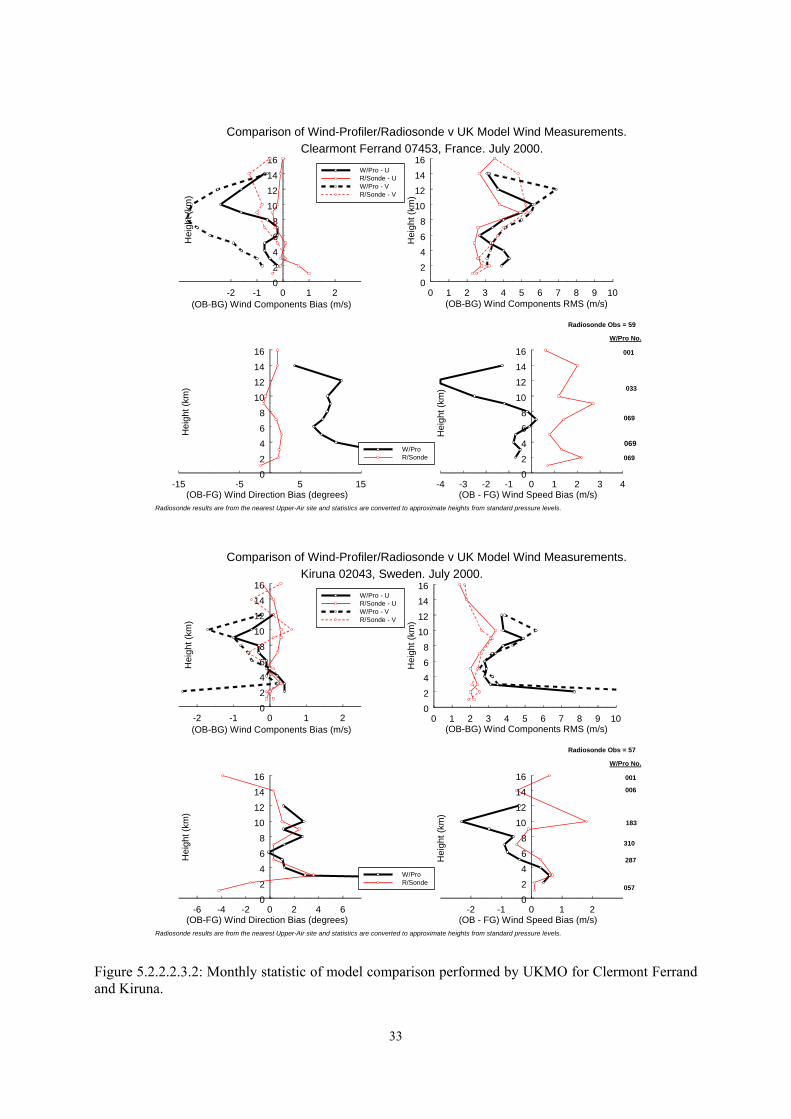
Figures 5.2.2.2.3.1 to 5.2.2.2.3.3 give an example of monthly statistic performed by Météo France and UKMO for different sites. UKMO statistics include also model comparisons against radiosoundings and give us the possibility to compare the accuracy of wind profiler and radiosondes. The bias of wind components, wind speed and wind direction as well as the rms-differences of wind component are plotted. The latter parameter contains information about systematic and random errors and is therefore a preferred value to estimate the accuracy (comparability). The rms differences show a different behaviour for the different systems. For some systems (Aberystwyth, Clermont Ferrand, Cabauw and Lindenberg) the rms differences have the same or only a little bit larger magnitude as for the comparison model � radiosonde. This indicates that the performance of wind profiler is comparable with that of radiosondes. Other systems showed in this month higher values of rms differences which could be an indication for some system trouble, problems in data processing or not optimally adjusted operation parameters. It must be noted that due to the continuous operation of wind profiler there is no chance for manual editing of real-time transmitted data. More advanced QC-algorithm can decrease the outlier rate.

Figure 5.2.2.2.3.4 shows the statistic of model comparison performed by Météo France. The bias and the standard deviation are plotted separately for four times of the day. The dotted vertical lines indicate a threshold for quality requirements of the model. It can be seen that the 482 MHz wind profiler (low mode) at Lindenberg fulfil the criterion at all heights, whereas larger deviations can be observed especially at lowest and upper heights for the 1290 MHz

32

system. An explanation could be ground clutter contamination at lowest heights and a decrease of the signal-to-noise ratio at upper heights.

-2 -1 0 1 2(OB-BG) Wind Components Bias (m/s)

0

2

4

6

8

10

12H

eigh

t (km

)W/Pro - UR/Sonde - U W/Pro - VR/Sonde - V

Comparison of Wind-Profiler/Radiosonde v UK Model Wind Measurements. Abersytwyth 03501(50MHz), UK. July 2000.

Radiosonde results are from the nearest Upper-Air site and statistics are converted to approximate heights from standard pressure levels.

0 1 2 3 4 5 6 7(OB-BG) Wind Components RMS (m/s)

0

2

4

6

8

10

12

Hei

ght (

km)

-6 -4 -2 0 2 4 6(OB-FG) Wind Direction Bias (degrees)

0

2

4

6

8

10

12

Hei

ght (

km)

W/ProR/Sonde

-2 -1 0 1 2(OB - FG) Wind Speed Bias (m/s)

0

2

4

6

8

10

12

Hei

ght (

km)

564

564

564

564

W/Pro No.

Radiosonde Obs = 44

564


02468

10121416

Hei

ght (

km)

W/Pro - UR/Sonde - U W/Pro - VR/Sonde - V

Comparison of Wind-Profiler/Radiosonde v UK Model Wind Measurements. Lindenberg 10394, Germany. July 2000.



02468

10121416

Hei

ght (

km)


02468

10121416

Hei

ght (

km)

W/ProR/Sonde


02468

10121416

Hei

ght (

km)

199

199

191

029

W/Pro No.

Radiosonde Obs = 118

063

Figure 5.2.2.2.3.1: Monthly statistic of model comparison performed by UKMO for Aberysthwyth and Lindenberg.

33


02468

10121416

Hei

ght (

km)


Comparison of Wind-Profiler/Radiosonde v UK Model Wind Measurements. Clearmont Ferrand 07453, France. July 2000.


0 1 2 3 4 5 6 7 8 9 10(OB-BG) Wind Components RMS (m/s)

02468

10121416

Hei

ght (

km)

-15 -5 5 15(OB-FG) Wind Direction Bias (degrees)

02468

10121416

Hei

ght (

km)

W/ProR/Sonde

-4 -3 -2 -1 0 1 2 3 4(OB - FG) Wind Speed Bias (m/s)

02468

10121416

Hei

ght (

km)

069

069

033

001

W/Pro No.

Radiosonde Obs = 59

069


02468

10121416

Hei

ght (

km)


Comparison of Wind-Profiler/Radiosonde v UK Model Wind Measurements. Kiruna 02043, Sweden. July 2000.



02468

10121416

Hei

ght (

km)


02468

10121416

Hei

ght (

km)

W/ProR/Sonde


02468

10121416

Hei

ght (

km)

287

310

183

001

W/Pro No.

Radiosonde Obs = 57

057

006

Figure 5.2.2.2.3.2: Monthly statistic of model comparison performed by UKMO for Clermont Ferrand and Kiruna.

34


012345678

Hei

ght (

km)


Comparison of Wind-Profiler/Radiosonde v UK Model Wind Measurements. Cabauw, Holland. July 2000.



012345678

Hei

ght (

km)


012345678

Hei

ght (

km)

W/ProR/Sonde


012345678

Hei

ght (

km)

113

083

043

024


W/Pro No.

115

-2 -1 0(OB-BG) Wind Components Bias (m/s)

012345678

Hei

ght (

km)


Comparison of Wind-Profiler/Radiosonde v UK Model Wind Measurements. Vienna 11035 (1290), Austria. July 2000.



012345678

Hei

ght (

km)

-10 -8 -6 -4 -2 0 2 4 6 8 10(OB-FG) Wind Direction Bias (degrees)

012345678

Hei

ght (

km)

W/ProR/Sonde


012345678

Hei

ght (

km)

116

113

067

000

W/Pro No.


203

Figure 5.2.2.2.3.3: Monthly statistic of model comparison performed by UKMO for Cabauw and Vienna.

35

Figure 5.2.2.2.3.4: Monthly statistic of model comparison performed by the Météo France.

36

2.2.3. Error sources for wind measurements

As it was demonstrated in the section before wind profiler /RASS are able to determine wind and temperature with high accuracy in most of their operation time. Nevertheless, there are situations where measurements can be disturbed by different system and/or environmental effects. Usually, disturbed measurements are eliminated by quality control algorithm.

In this section an overview of the most relevant error sources should be given, which occur independent from the system. Several figures from different stages of signal processing illustrate the errors and can help to identify error sources for any users.

2.2.3.1. Unwanted backscattering processes

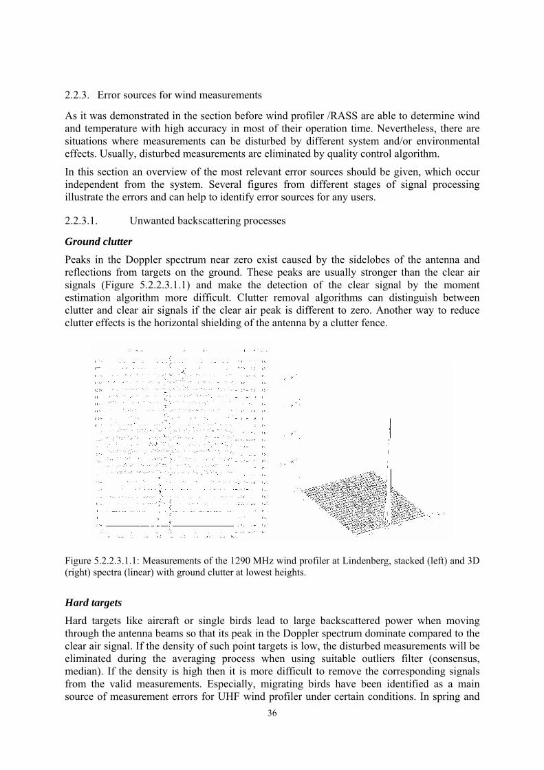
Ground clutter Peaks in the Doppler spectrum near zero exist caused by the sidelobes of the antenna and reflections from targets on the ground. These peaks are usually stronger than the clear air signals (Figure 5.2.2.3.1.1) and make the detection of the clear signal by the moment estimation algorithm more difficult. Clutter removal algorithms can distinguish between clutter and clear air signals if the clear air peak is different to zero. Another way to reduce clutter effects is the horizontal shielding of the antenna by a clutter fence.

Figure 5.2.2.3.1.1: Measurements of the 1290 MHz wind profiler at Lindenberg, stacked (left) and 3D (right) spectra (linear) with ground clutter at lowest heights.

Hard targets Hard targets like aircraft or single birds lead to large backscattered power when moving through the antenna beams so that its peak in the Doppler spectrum dominate compared to the clear air signal. If the density of such point targets is low, the disturbed measurements will be eliminated during the averaging process when using suitable outliers filter (consensus, median). If the density is high then it is more difficult to remove the corresponding signals from the valid measurements. Especially, migrating birds have been identified as a main source of measurement errors for UHF wind profiler under certain conditions. In spring and

37

autumn, mostly during fair weather conditions and especially at night-time, bird migration disturb wind profiler measurements (Ecklund et al., 1990; Wilczak et al., 1995). For the 1290 MHz wind profiler at Lindenberg about 2 % of all comparisons with rawinsondes show unrealistic large differences when the wind profiler is operating in high mode (Engelbart et al., 1998). Figure 5.2.2.3.1.2 shows an occasion when the movement of birds has contaminated measurements during the night.

Figure 5.2.2.3.1.2: Time-height cross-section of wind barbs of the 1290 MHz wind profiler at Lindenberg showing night-time bird migration. Wind are contaminated between 01 and 03 UTC and 18 and 23 UTC.

In autumn at Lindenberg the bird migration direction is from Northeast to Southwest during the night. The sharp turn of direction can be seen clearly at sun rise and sun set. Due to the temporal consistence of these disturbances, automatical quality algorithm are usually not able to remove bird contaminated measurements. The contamination effect depends mainly on pulse volume in connection with migration density and velocity as well as on the time needed for spectral averaging. That is the reason that in the low mode with a smaller pulse volume the effect is significant lower, when the density of migrating birds is low.

The application of a more advanced spectral processing like the Intermittent Clutter Reduction Algorithm (ICRA) (Merritt, 1995) instead of the Mean algorithm can reduce the effect of bird contamination significantly.

Precipitation Under some conditions precipitation can lead to the following sources of errors: • During precipitation Bragg scattering and Rayleigh scattering may have similar

magnitude. In such cases (single) moment estimation algorithms may not clearly identify one peak, and the reported first moment may lie between the Bragg and Rayleigh peaks,

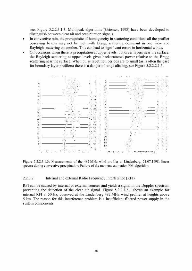
38

see. Figure 5.2.2.3.1.3. Multipeak algorithms (Griesser, 1998) have been developed to distinguish between clear air and precipitation signals.

• In convective rain, the prerequisite of homogeneity in scattering conditions all the profiler observing beams may not be met, with Bragg scattering dominant in one view and Rayleigh scattering on another. This can lead to significant errors in horizontal winds.

• On occasions when there is precipitation at upper levels, but dryer layers near the surface, the Rayleigh scattering at upper levels gives backscattered power relative to the Bragg scattering near the surface. When pulse repetition periods are to small (as is often the case for boundary layer profilers) there is a danger of range aliasing, see Figure 5.2.2.2.1.5.

Figure 5.2.2.3.1.3: Measurements of the 482 MHz wind profiler at Lindenberg, 21.07.1998: linear spectra during convective precipitation: Failure of the moment estimation FM-algorithm.

2.2.3.2. Internal and external Radio Frequency Interference (RFI)

RFI can be caused by internal or external sources and yields a signal in the Doppler spectrum preventing the detection of the clear air signal. Figure 5.2.2.3.2.1 shows an example for internal RFI at 50 Hz, observed at the Lindenberg 482 MHz wind profiler at heights above 5 km. The reason for this interference problem is a insufficient filtered power supply in the system components.

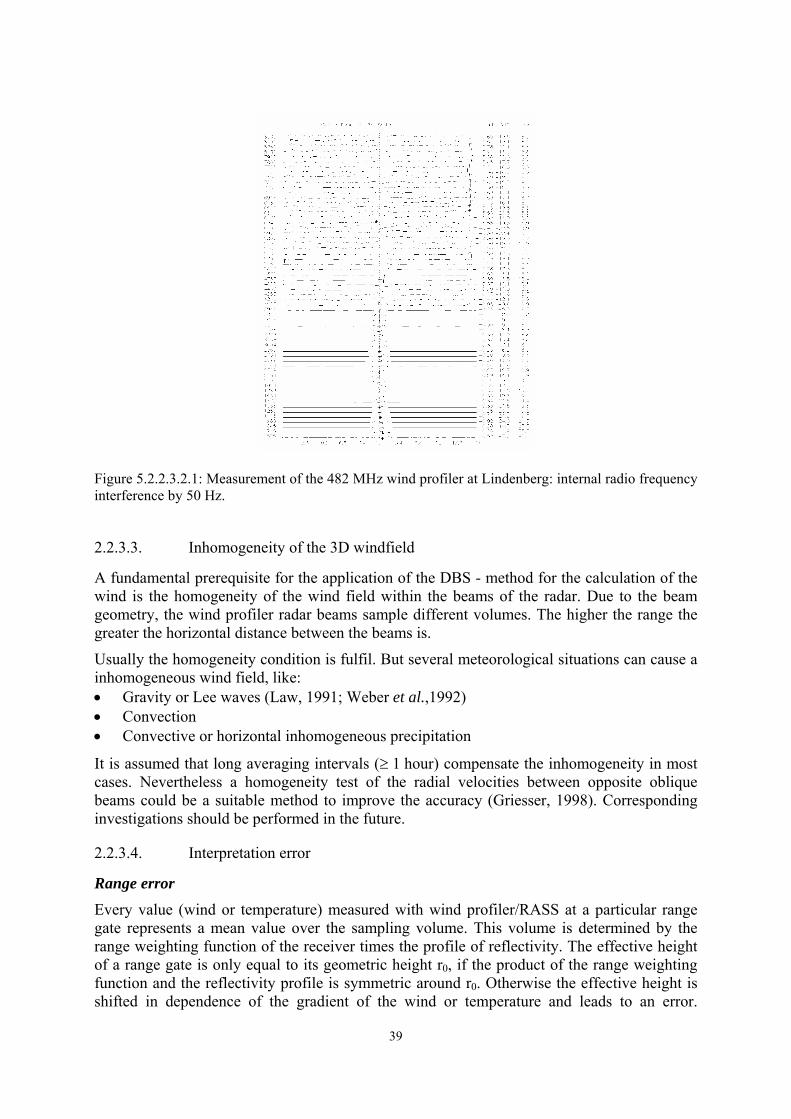
39

Figure 5.2.2.3.2.1: Measurement of the 482 MHz wind profiler at Lindenberg: internal radio frequency interference by 50 Hz.

2.2.3.3. Inhomogeneity of the 3D windfield

A fundamental prerequisite for the application of the DBS - method for the calculation of the wind is the homogeneity of the wind field within the beams of the radar. Due to the beam geometry, the wind profiler radar beams sample different volumes. The higher the range the greater the horizontal distance between the beams is.

Usually the homogeneity condition is fulfil. But several meteorological situations can cause a inhomogeneous wind field, like: • Gravity or Lee waves (Law, 1991; Weber et al.,1992) • Convection • Convective or horizontal inhomogeneous precipitation

It is assumed that long averaging intervals (≥ 1 hour) compensate the inhomogeneity in most cases. Nevertheless a homogeneity test of the radial velocities between opposite oblique beams could be a suitable method to improve the accuracy (Griesser, 1998). Corresponding investigations should be performed in the future.

2.2.3.4. Interpretation error

Range error Every value (wind or temperature) measured with wind profiler/RASS at a particular range gate represents a mean value over the sampling volume. This volume is determined by the range weighting function of the receiver times the profile of reflectivity. The effective height of a range gate is only equal to its geometric height r0, if the product of the range weighting function and the reflectivity profile is symmetric around r0. Otherwise the effective height is shifted in dependence of the gradient of the wind or temperature and leads to an error.

40

Systematic differences up to 1 K have been found for RASS temperature measurements (Goersdorf and Lehmann, 2000) and up to 0.2 m.s-1 for wind measurements (Muschinski et al., 1999) (see also 5.2.1.3, Figure 5.2.2.1.1).

Finite volume effect Sharp vertical variations of the backscattered coefficient caused by thin turbulent layers can be the reason that the backscattered signal is not centred around the zenith angle. This effect yields errors in the calculation of the horizontal wind components and was described by Fukao et al. (1988) in detail on the base of the MU radar in Japan. An estimation of this error for any profiler fails because information about the reflectivity with a high vertical resolution are missing.

2.2.3.5. Unsuitable parameter adjustments

Range-aliasing

Doppler radars usually operate with a constant pulse repetition time Ts. The range of the sampling interval can be calculated by

2τc sr = (5.2.2.3.5.1)

where c is the speed of light and τs is the range time delay. For the case that scatters have a range larger than c Ts /2, their echoes are received after the next pulse is transmitted. When the echo is strong enough, the echoes returned from higher ranges are interpreted as echoes from lower ranges.

The maximum unambiguous range ra is a function of Ts:

2

sa

cTr = (5.2.2.3.5.2)

Especially for boundary layer wind profilers range aliasing could be an error source, when the Ts was chosen as too small. For example during precipitation events the reflectivity at upper ranges can increase and yield strong backscattered signals from heights greater than ra.

Velocity-aliasing

Velocity aliasing occurs if the Nyquist-velocity is smaller than the radial velocity. In such situations the Doppler frequency (fd = 2 f vr /c) is so high that the signal cannot resolved unambiguous. It is interpreted as a lower frequency and consequently as a lower velocity. The Nyquist-velocity is

s

a Tv 4λ

= (5.2.2.3.5.3)

Velocity aliasing can be observed in situations with high wind speeds and a wind direction parallel to the connection line of the beams (Figure 5.2.2.3.5.1).

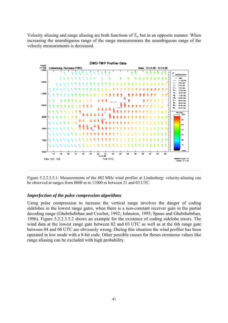
41

Velocity aliasing and range aliasing are both functions of Ts, but in an opposite manner. When increasing the unambiguous range of the range measurements the unambiguous range of the velocity measurements is decreased.

Figure 5.2.2.3.5.1: Measurements of the 482 MHz wind profiler at Lindenberg: velocity-aliasing can be observed at ranges from 8000 m to 11000 m between 21 and 03 UTC.

Imperfection of the pulse compression algorithms Using pulse compression to increase the vertical range involves the danger of coding sidelobes in the lowest range gates, when there is a non-constant receiver gain in the partial decoding range (Ghebrhebrhan and Crochet, 1992; Johnston, 1995; Spano and Ghebrhebrhan, 1996). Figure 5.2.2.3.5.2 shows an example for the existence of coding sidelobe errors. The wind data at the lowest range gate between 02 and 03 UTC as well as at the 6th range gate between 04 and 06 UTC are obviously wrong. During this situation the wind profiler has been operated in low mode with a 8-bit code. Other possible causes for theses erroneous values like range aliasing can be excluded with high probability.

42

Figure 5.2.2.3.5.2: Measurements of the 482 MHz wind profiler at Lindenberg: measuring error due to coding sidelobes.

2.2.3.6. Hardware faults

Hardware faults can be also the reason for measurement errors. The technical characteristics of the antenna and its temporal stability is fundamental for the evaluation of valid wind data. The detection of such failures is often difficult and depends on the extent of the hardware failure. Therefore a comprehensive monitoring of critical system components is recommended (see also section maintenance).

2.2.4. Error sources for temperature measurements

RASS systems use for the calculation of virtual temperature profiles the following equation:

2a

dv c

RM

Tγ

= (5.2.2.4.1)

where ca is the speed of sound measured by the wind profiler, Md is the molecular weight of dry air (= 28.96 kg.kmol-1), γ is the ratio of specific heats (= 1.4) and R (= 8314.44 J.mol-1K-1) is the universal gas constant. Comparisons between RASS temperature profiles calculated with the given formula including the constants and radiosonde temperature profiles performed at several sites show a height dependent systematic bias of RASS-measured profiles . Especially at the lowest range gates, a height-dependent bias remained resulting in an

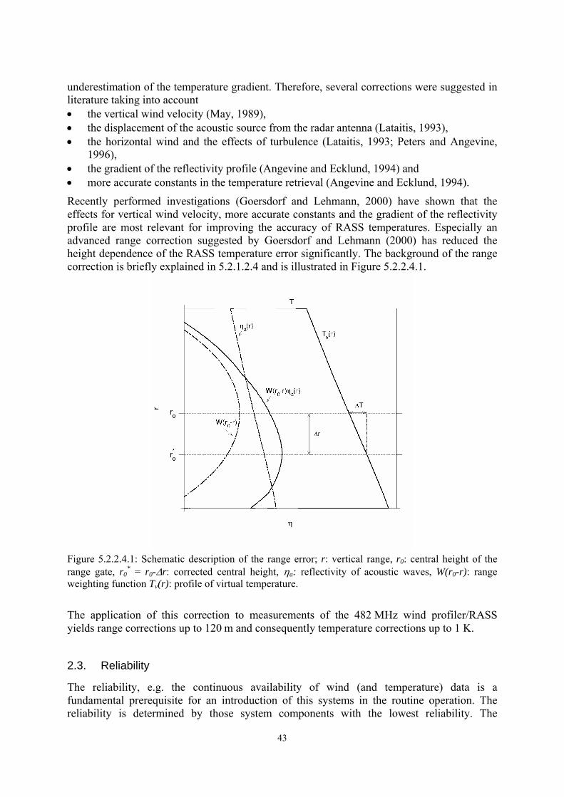
43

underestimation of the temperature gradient. Therefore, several corrections were suggested in literature taking into account • the vertical wind velocity (May, 1989), • the displacement of the acoustic source from the radar antenna (Lataitis, 1993), • the horizontal wind and the effects of turbulence (Lataitis, 1993; Peters and Angevine,

1996), • the gradient of the reflectivity profile (Angevine and Ecklund, 1994) and • more accurate constants in the temperature retrieval (Angevine and Ecklund, 1994).

Recently performed investigations (Goersdorf and Lehmann, 2000) have shown that the effects for vertical wind velocity, more accurate constants and the gradient of the reflectivity profile are most relevant for improving the accuracy of RASS temperatures. Especially an advanced range correction suggested by Goersdorf and Lehmann (2000) has reduced the height dependence of the RASS temperature error significantly. The background of the range correction is briefly explained in 5.2.1.2.4 and is illustrated in Figure 5.2.2.4.1.

Figure 5.2.2.4.1: Schematic description of the range error; r: vertical range, r0: central height of the range gate, r0

* = r0-∆r: corrected central height, ηa: reflectivity of acoustic waves, W(r0-r): range weighting function Tv(r): profile of virtual temperature.

The application of this correction to measurements of the 482 MHz wind profiler/RASS yields range corrections up to 120 m and consequently temperature corrections up to 1 K.

2.3. Reliability

The reliability, e.g. the continuous availability of wind (and temperature) data is a fundamental prerequisite for an introduction of this systems in the routine operation. The reliability is determined by those system components with the lowest reliability. The

44

availability of data depends in the end on a lot of factors, like repair time, maintenance and a monitoring of important system functions in order to prevent system failures. Increased availability can be achieved also by a permanent improvement of system components in a close co-operation with the manufactures.

Valuable experiences in view of the reliability of wind profiler/RASS have been gathered at many European wind profiler sites during continuous operation in resent years. Of course, such experiences are related to the specific systems and therefore, only some general statements can be given.

One remarkable and common hardware problem are faulty relays in phase shifter have occurred at many profiler sites. More relevant are disturbances by the environmental conditions. Spectral peaks due to ground clutter contaminate the spectra at the lowest range gates on more than the half of all European profiler sites. In many cases only one direction is affected by ground clutter echoes. UHF-wind profiler measurements are frequently disturbed by migration, especially in spring and autumn, where the bird density exceeds a critical value, which depends on the profiler configuration.

VHF- wind profilers are more sensitive to scattering from larger objects like aircraft, which were found to give spurious peaks at two CWINDE sites.

Occasionally, also software including network problems are the reason for data losses.

Figure 5.2.3.1 shows an example of reliability for the Lindenberg systems and its temporal development.

Figure 5.2.3.1: Available (squares) and real-time transmitted messages (triangles) of both Lindenberg wind profiler/RASS-systems.

3. Quality evaluation

3.1. Introduction

This section will describe the techniques used by the CWINDE network hub to derive routine products on availability and quality for the operators of the systems contributing to network.

45

Operators of the systems connected to CWINDE receive regular monitoring reports giving monthly details on the messages received, reported wind height coverage and summaries of the comparison of observations with short term weather forecast fields. The quality evaluation procedures are mostly developments of methods originally summarised in Chapter 7 of the COST 74 Final Report (1994). Developments in this area have taken longer than expected during COST 76, because the staffing of routine CWINDE network operations consumed higher staff resources than originally estimated.

3.2. Data availability

Data from the profiler sites co-operating with CWINDE are displayed in various formats on the CWINDE web page with plots updated every 30 minutes. This enables operators to check directly that correct data are being transmitted to Bracknell.

A presentation of all current profiler wind data in the form of a thumbnail set is used by the project office to monitor data being received, so that any communications problems can be quickly resolved.

3.3. Identification of anomalous measurements

As noted in Section 5.2, wind profiler measurements can have large measurement anomalies. Problems will occur if the operators have not adjusted the system configuration to minimise the effects of ground clutter, sea clutter, intermittent sources of radio interference or breakthrough from main power supply frequencies when signals are very weak in the lowest range gates.

The CWINDE web display plots are used to identify data anomalies. Figure 5.3.3.1 shows a plot from the Innsbruck profiler at an early stage of its operation. Here, there were some spurious wind reports in the lowest range gates and also some spurious reports were escaping the system quality evaluation software at upper levels. The very strong winds in the lowest range gates may have been the result of mains pick up when atmospheric signals were very weak. The spurious signals at upper levels between 04 and 05 UTC may have been caused by inadequate data samples. The rate of occurrence of these types of errors can be quantified and operating procedures adjusted or referred back to the manufacturer to rectify the problem. This plot does not typify the subsequent performance of this radar.

The type of problem caused by the migration of birds in the UK in spring can be seen in Figures 5.3.3.2.a) and 5.3.3.2.b). Experience has shown that bird migration at UK profiler sites is mostly a problem with redwings migrating from Ireland to Russia in spring and returning to the western coasts in autumn. On the West Coast of the British Isles in spring, the birds are most commonly seen for two or three hours after sunset, migrating on clear days with winds blowing towards the east. The birds fly at about 10 to 15 m.s-1 relative to the air.

When bird echoes are dominating the profiler consensus over the UK in spring, the reported westerly wind speed has a positive bias of about 10 to 15 m.s-1. Thus, in Figure 5.3.3.2.a), whilst the winds at 1.5 km were increasing with time during the day, the network operator would be alerted when winds suddenly jumped to values in excess of 25 m.s-1 just after sunset. The signal power and vertical velocity plots in Figure 5.3.3.2.b) show very strong increase in signal to noise between 18 UTC and midnight, without the distribution of vertical velocity that would usually be associated when precipitation was producing such a strong signal.

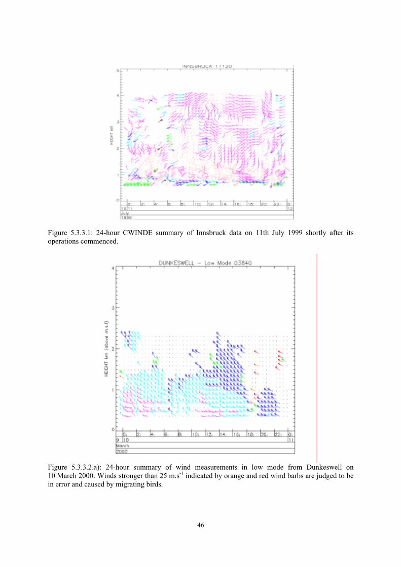
46

Figure 5.3.3.1: 24-hour CWINDE summary of Innsbruck data on 11th July 1999 shortly after its operations commenced.

Figure 5.3.3.2.a): 24-hour summary of wind measurements in low mode from Dunkeswell on 10 March 2000. Winds stronger than 25 m.s-1 indicated by orange and red wind barbs are judged to be in error and caused by migrating birds.

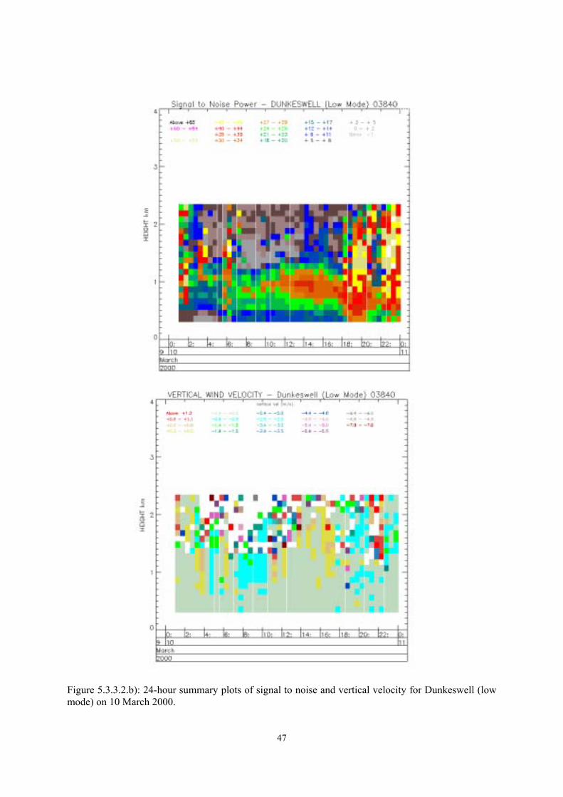
47

Figure 5.3.3.2.b): 24-hour summary plots of signal to noise and vertical velocity for Dunkeswell (low mode) on 10 March 2000.

48

For most of the period of very strong signal, no winds were reported in Figure 5.3.3.2.a). This was because the contamination introduced by the birds was not so high as to completely dominate the observations, and the quality control software threw the measurements out as too variable. Only a few samples were dominated by the bird echoes and produced a satisfactory consensus and hence erroneous winds.

3.4. Quality evaluation techniques

3.4.1. Comparisons with numerical forecast fields

Estimation of wind measurement accuracy from comparison with model fields has been discussed in some detail in Section 5.2. For a profiler working correctly, with good quality control software in place, comparison against NWP (Numerical Weather Prediction) model fields is a useful method for checking for systematic bias in wind direction or speed. Figure 5.3.4.1.1 shows wind direction and wind speed bias compared to the Met. Office model�s first guess (six hour) forecast field, averaged for a month. Comparisons with the measurements from the nearest radiosonde station are also presented to check whether the forecast fields are reliable or in error to some extent. The results in Figure 5.3.4.1.1 are for the month before the July 2000 results shown in Figure 5.2.2.2.3.3. The wind speed bias results for radiosonde and profiler were similar for both June and July. The wind profiler measurements were about 1.5 m.s-1 lower than the radiosondes with respect to the model fields. Whether this was caused by local variation in wind fields, the accuracy of the model forecast or a malfunction of radiosonde or profiler would require further investigation. The difference in wind direction between the model forecast and profiler observations was similar for the two months, but the radiosonde direction bias with respect to the model differed by about 4 degrees between the two months. On average, the wind profiler directions at 2 km were lower than those of the radiosonde system by about 3 degrees.

Figure 5.3.4.1.1: Wind speed and direction bias against the Met. Office (UK) first guess fields for Vienna, June 2000.

However, to be sure about relatively small wind speed and direction biases it is necessary to examine the performance for much longer periods than a month. In Vienna, the wind profiler is some distance from the radiosonde launch site. In flat terrain it is relatively safe to use the forecast fields as a cross reference between neighbouring radiosonde and profiler locations,

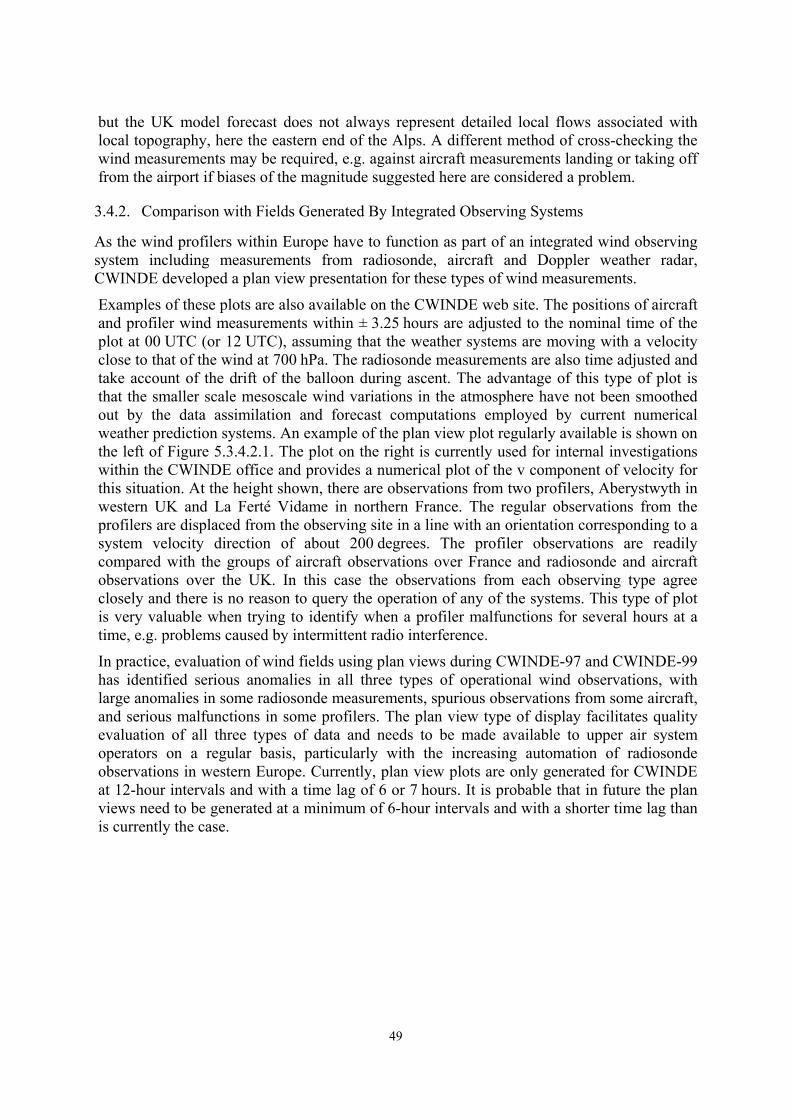
49

but the UK model forecast does not always represent detailed local flows associated with local topography, here the eastern end of the Alps. A different method of cross-checking the wind measurements may be required, e.g. against aircraft measurements landing or taking off from the airport if biases of the magnitude suggested here are considered a problem.

3.4.2. Comparison with Fields Generated By Integrated Observing Systems

As the wind profilers within Europe have to function as part of an integrated wind observing system including measurements from radiosonde, aircraft and Doppler weather radar, CWINDE developed a plan view presentation for these types of wind measurements.

Examples of these plots are also available on the CWINDE web site. The positions of aircraft and profiler wind measurements within ± 3.25 hours are adjusted to the nominal time of the plot at 00 UTC (or 12 UTC), assuming that the weather systems are moving with a velocity close to that of the wind at 700 hPa. The radiosonde measurements are also time adjusted and take account of the drift of the balloon during ascent. The advantage of this type of plot is that the smaller scale mesoscale wind variations in the atmosphere have not been smoothed out by the data assimilation and forecast computations employed by current numerical weather prediction systems. An example of the plan view plot regularly available is shown on the left of Figure 5.3.4.2.1. The plot on the right is currently used for internal investigations within the CWINDE office and provides a numerical plot of the v component of velocity for this situation. At the height shown, there are observations from two profilers, Aberystwyth in western UK and La Ferté Vidame in northern France. The regular observations from the profilers are displaced from the observing site in a line with an orientation corresponding to a system velocity direction of about 200 degrees. The profiler observations are readily compared with the groups of aircraft observations over France and radiosonde and aircraft observations over the UK. In this case the observations from each observing type agree closely and there is no reason to query the operation of any of the systems. This type of plot is very valuable when trying to identify when a profiler malfunctions for several hours at a time, e.g. problems caused by intermittent radio interference.

In practice, evaluation of wind fields using plan views during CWINDE-97 and CWINDE-99 has identified serious anomalies in all three types of operational wind observations, with large anomalies in some radiosonde measurements, spurious observations from some aircraft, and serious malfunctions in some profilers. The plan view type of display facilitates quality evaluation of all three types of data and needs to be made available to upper air system operators on a regular basis, particularly with the increasing automation of radiosonde observations in western Europe. Currently, plan view plots are only generated for CWINDE at 12-hour intervals and with a time lag of 6 or 7 hours. It is probable that in future the plan views need to be generated at a minimum of 6-hour intervals and with a shorter time lag than is currently the case.

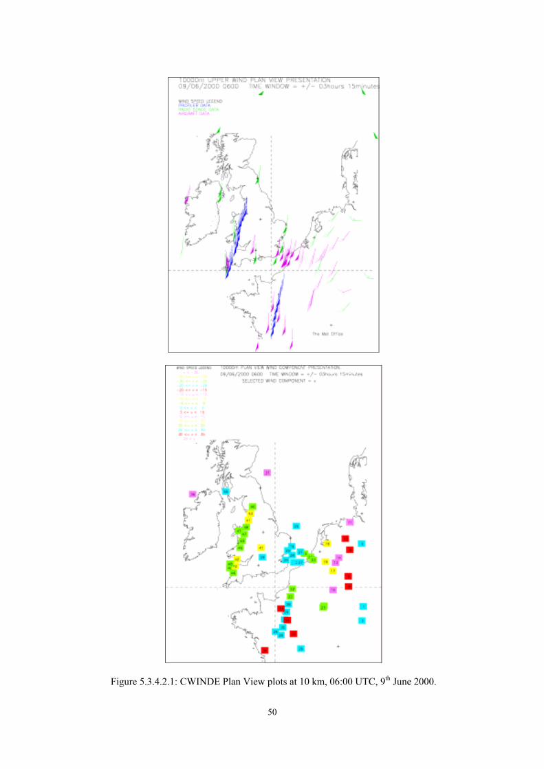
50

Figure 5.3.4.2.1: CWINDE Plan View plots at 10 km, 06:00 UTC, 9th June 2000.

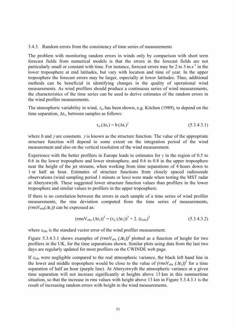
51

3.4.3. Random errors from the consistency of time series of measurements

The problem with monitoring random errors in winds only by comparison with short term forecast fields from numerical models is that the errors in the forecast fields are not particularly small or constant with time. For instance, forecast errors may be 2 to 3 m.s-1 in the lower troposphere at mid latitudes, but vary with location and time of year. In the upper troposphere the forecast errors may be larger, especially at lower latitudes. Thus, additional methods can be beneficial in identifying changes in the quality of operational wind measurements. As wind profilers should produce a continuous series of wind measurements, the characteristics of the time series can be used to derive estimates of the random errors in the wind profiler measurements.

The atmospheric variability in wind, τu, has been shown, e.g. Kitchen (1989), to depend on the time separation, ∆t1, between samples as follows: τu (∆t1) = b (∆t1)γ (5.3.4.3.1) where b and γ are constants. γ is known as the structure function. The value of the appropriate structure function will depend to some extent on the integration period of the wind measurement and also on the vertical resolution of the wind measurement.

Experience with the better profilers in Europe leads to estimates for γ in the region of 0.5 to 0.6 in the lower troposphere and lower stratosphere, and 0.6 to 0.8 in the upper troposphere near the height of the jet streams, when working from time separations of 4 hours down to 1 or half an hour. Estimates of structure functions from closely spaced radiosonde observations (wind sampling period 1 minute or less) were made when testing the MST radar at Aberystwyth. These suggested lower structure function values than profilers in the lower troposphere and similar values to profilers in the upper troposphere.

If there is no correlation between the errors in each sample of a time series of wind profiler measurements, the rms deviation computed from the time series of measurements, (rmsVobs(∆t1)) can be expressed as: (rmsVobs (∆t1))2 = (τu (∆t1))2 + 2. (εobs)2 (5.3.4.3.2) where εobs is the standard vector error of the wind profiler measurement.

Figure 5.3.4.3.1 shows examples of (rmsVobs (∆t1))2 plotted as a function of height for two profilers in the UK, for the time separations shown. Similar plots using data from the last two days are regularly updated for most profilers on the CWINDE web page.

If εobs were negligible compared to the real atmospheric variance, the black left hand line in the lower and middle troposphere would be close to the value of (rmsVobs (∆t1))2 for a time separation of half an hour (purple line). At Aberystwyth the atmospheric variance at a given time separation will not increase significantly at heights above 13 km in this summertime situation, so that the increase in rms values with height above 13 km in Figure 5.3.4.3.1 is the result of increasing random errors with height in the wind measurements.

52

Figure 5.3.4.3.1: RMS averages computed from 48-hour time series of observations for time separations between 30 minutes and 4 hours from Dunkeswell (1290 MHz) on 22/6/2000 and Aberystwyth (46 MHz) on 19/7/2000.

The values of (rmsVobs (∆t1))2 for time separations of 4 hours and 1 hour (or half an hour) can be used to produce an estimate of the random error in the observations, using Equations (5.3.4.3.1) and (5.3.4.3.2) provided the relevant value of the structure function is known. In some situations the solution for the random error is very insensitive to the assumed structure function, and in others it is not. Thus, it was decided to generate a quality evaluation product

53

showing the random errors as a function of height, with error values computed for a reasonable range of structure function values. One of these plots is shown in Figure 5.3.4.3.2 for the Aberystwyth profiler, where time separations of 4 hour and 0.4 hours have been used for the computations. The resulting values of atmospheric variance at 4 hours and 0.4 hours for each structure function used in the error estimates are shown as a function of height in Figure 5.3.4.3.3.

On this occasion the random errors in wind were of similar magnitude to the atmospheric variance at 0.4 hours time separation, and the error estimates were not very dependent on the structure function that was assumed. It is necessary to check that the resultant atmospheric variations vary in a realistic manner with height. Here, there were no significant problems below 16 km, but the atmospheric variation appears to be increasing with height at heights above 16 km. It is probable that this is because some of the random errors at these heights were correlated over periods longer than 0.4 hours, but not over periods as long as 4 hours. Thus, the true random error estimates above 16 km in Figure 5.3.4.3.2 should probably be larger than shown, with true atmospheric variance lower than shown. In any case, signal to noise limitations at longer ranges in this operational mode start to impose limits on the MST radar accuracy at heights above 14 km in wind at 0.4 hours, so the resultant error estimates were not critically dependent on the structure function.

0,00

0,50

1,00

1,50

2,00

2,50

3,00

3,50

4,00

0 2000 4000 6000 8000 10000 12000 14000 16000 18000

Height above sea level [m]

RM

S ve

ctor

err

or [

ms-

1]

Error,s.f.=0.5 Error,s.f.=0.6 Error,s.f.=0.7 Error,s.f.=0.8

Figure 5.3.4.3.2: Estimates of random error as a function of height for a time series of a week in March 1999 from the Aberystwyth MST radar during CWINDE-99, for the structure functions shown.

54

0,00

1,00

2,00

3,00

4,00

5,00

6,00

7,00

8,00

9,00

0 2000 4000 6000 8000 10000 12000 14000 16000 18000

Height above sea level [m]

RM

S ve

ctor

diff

eren

ce [

ms-

1]s.f.=0.5,0.4 hour s.f.=0.6,0.4 hour s.f.=0.7,0.4hour s.f.=0.8,0.4 hour

s.f.=0.5,4 hour s.f.=0.6,4 hour s.f.=0.7,4hour s.f.=0.8,4 hour

Figure 5.3.4.3.3: Atmospheric variance for 0.4-hour and 4-hour time separations (left) from a time series of measurements for a week in March 1999, Aberystwyth MST radar, for the structure functions indicated.

3.5. Random error results from CWINDE-99

Time series of measurements from the profilers participating in CWINDE-99 were analysed using the error estimate technique in 5.3.4.3, and assuming a similar structure function for each radar site.

The error estimates for the 50 MHz VHF profilers plus Lindenberg operating at 482 MHz are shown in Figure 5.3.5.1 with the associated atmospheric variation at time separations of 4 and 1 hour in Figure 5.3.5.2. Aberystwyth and Kiruna measurements had the largest random errors during this sample period. Both radars have subsequently improved in this aspect of performance. Lindenberg measurements clearly had the lowest random errors in this group of radars, and the solution for random error at Lindenberg was very sensitive to the structure function that was assumed. The variation of atmospheric variation with height at Aberystwyth and Lindenberg was nearly identical. On the other hand, La Ferté Vidame measured much less variation at 9 and 10 km than Lindenberg and Aberystwyth. This suggests that La Ferté Vidame may not have adequately sampled some of the real atmospheric variation at these heights. Kiruna and Andenes were much further north and would not be expected to show the same atmospheric variation.

The equivalent error estimates for the 1 GHz profilers operating in CWINDE-99 can be found in Figure 5.3.5.3, with the associated atmospheric variation estimates in Figure 5.3.5.4. In these figures all the profilers apart from Karlsruhe were of similar design and origin. However, the measurement quality is clearly not identical with random errors from similar

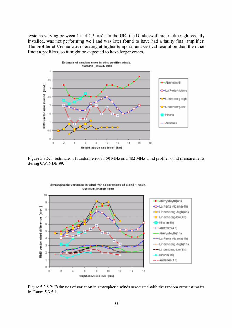
55

systems varying between 1 and 2.5 m.s-1. In the UK, the Dunkeswell radar, although recently installed, was not performing well and was later found to have had a faulty final amplifier. The profiler at Vienna was operating at higher temporal and vertical resolution than the other Radian profilers, so it might be expected to have larger errors.

Figure 5.3.5.1: Estimates of random error in 50 MHz and 482 MHz wind profiler wind measurements during CWINDE-99.

Figure 5.3.5.2: Estimates of variation in atmospheric winds associated with the random error estimates in Figure 5.3.5.1.

56

Figure 5.3.5.3: Estimates of random error in 1 GHz wind profiler wind measurements during CWINDE-99.

Figure 5.3.5.4: Estimates of variation in atmospheric winds associated with the random error estimates in Figure 5.3.5.3.

57

Figure 5.3.5.5: Estimates of random error in NOAA Profiler Network wind profiler wind measurements during summer 2000.

Atmospheric variance in wind in Figure 5.3.5.4 ought to have been similar at Cabauw, Camborne and Dunkeswell as coastal sites. Lindenberg was further inland and Payerne and Vienna were influenced by the Alps. Vienna showed the greatest variability at low levels. This needs to be investigated further to see if this was real or whether it was a result of instrument malfunction. Once, the wind characteristics introduced by the topography surrounding the site are established, then it should be easier to keep track of the observation quality.

In order to put the performance of the European profilers in context, the measurements of the NOAA Profiler network were assessed for a week in summer 2000 using the same technique. The results of the random error estimates are shown in Figure 5.3.5.5, where the NOAA network was arbitrarily grouped according to geographical location. Here, the estimated errors fell within the range 1 to 2 m.s-1.

3.6. Summary

There is still some scope for improving the feedback of quality evaluation results to operators and educating them in the techniques of identifying wind measurement errors.

Potentially between 15 and 18 European profilers could regularly input wind measurements to the users, but currently only about ten are considered of acceptable measurement quality by the users. The main problem seems to be intermittent large anomalies, rather than a failure to measure with low random errors most of the time.

58

Within Europe there are still wind profilers that are operated for much of the year, but have not yet joined with CWINDE. The experience of COST 76 is that profiler radars do fail fairly regularly during operation, and most operators do not recognise the symptoms very quickly. Many instrument scientists are not well versed in the techniques of data evaluation. Thus, it is recommended that all operators within Europe do make use of the monitoring facilities offered by CWINDE to minimise the chance of operating with a substandard system over long periods of time.

4. Maintenance

4.1. Introduction

Wind Profiler Radar (WPR) and Radio-Acoustic Sounding Systems (RASS) are complex meteorological remote sensing systems consisting of different components like antenna, transmitter, receiver, and data processor. To guarantee an undisturbed running of these systems, a more or less extensive maintenance has to be realised. The efforts necessary for the maintenance of WPR and/or RASS depend on the applications: • The maintenance of experimental WPR and/or RASS prototypes is carried out in many

cases from specialists who have been involved in the development of these systems. These specialist are very close to the special characteristics of the system and can make the maintenance very effective based on their knowledge of the system development. The requirements for the maintenance of such kind of systems are very low because the development specialists are available for maintenance also during the use of this system for different scientific investigations.

• The applications of production model WPR and/or RASS for scientific investigations depend on the special conditions which are given in the institution or organisation using these systems. Generally, scientific institutions using remote sensing systems have technical specialists with high knowledge in WPR and RASS technology. Therefore, the requirements for the maintenance of WPR/RASS in scientific institution is low under the condition that these technical specialists are available for maintenance.

• The requirements for the maintenance increase, if the WPR and/or RASS have to operate unattended and continuously under operational conditions of a weather service. The operational use of WPR and/or RASS requires a number of special conditions which have to be fulfilled to guarantee the operational use over a long period. The basis for the maintenance of operationally used WPR and/or RASS are the automatic remote monitoring of all important system functions to allow a comprehensive remote system check as well as the diagnosis of the WPR and/or RASS technical status. The effort for the maintenance should be as small as possible on the one hand and as comprehensive as necessary to ensure accuracy, availability, and high reliability of the WPR/RASS on the other hand.

This section is focused on the requirements and conditions for remote monitoring, diagnosis, and maintenance of operational WPR-/RASS-systems used in meteorological networks.

4.2. Requirements for maintenance

WPR and/or RASS for routine applications are required to operate unattended and continuously under nominal conditions for a period of at least 10 years. The expected mean

59

time between failures (MTBF) is required to be superior to 5000 hours (Gilet, 1994). Furthermore, the staff necessary for the maintenance of these systems should be as small as possible. One may infer from that the requirements for maintenance of WPR and RASS:

• The operational use of WPR/RASS in meteorological networks requires a high system reliability which is determined by those system components with the lowest reliability. Therefore, the MTBF of all single system components should be significant greater than the required MTBF for the WPR/RASS, e.g. 10�000 to 50�000 hours.

• Due to the fact that operational WPR and RASS are often installed in remote areas and the requirement of low maintenance efforts, WPR and/or RASS have to be equipped with a remote monitoring unit for the important system parameters. The comprehensive remote monitoring of significant system parameters is an important prerequisite for an effective system watch and diagnosis. Based on remote monitoring of the essential parameters, the recognition of any faults that may occur is possible and a corresponding repair can be arranged.

• The necessary preventive maintenance has to be simple and manageable based on a modular system configuration. The frequency of maintenance carried out preventively for one WPR/RASS should not exceed two times per year each with an average necessary time period of about 4 to 8 hours.

The above called requirements are the basis for an effective and simple concept of maintenance of WPR and RASS. Such concept has to ensure that an automatic remote system watch is implemented to identify disturbances of system parameters as early as possible and to arrange routine maintenance if it is necessary. Furthermore, it has to guarantee the perfect running of all system functions as well as the measuring accuracy by preventive maintenance.

4.3. Remote monitoring and diagnosis of WPR/RASS

The basis for the maintenance of WPR/RASS implemented in a network should be an automatic remote monitoring of all important system functions to allow a comprehensive system check as well as a diagnosis of the WPR state at three different levels: • A technical system level based on technical parameters being essentially for the system

functions. • A signal processing level giving the possibility to have an insight in spectrum or

momentum data. • A output level based on the output data transmitted to the users.

Corresponding these levels, the remote monitoring has to be integrated within the WPR/RASS processing unit. The maintenance staff needs the access to the different levels as well as subordinated sublevels (e.g. voltages and currents of the transmitter or other units) by a flexible monitoring and diagnosis concept in order to get a complete overview about all available system parameters and data. Corresponding this concept, a remote monitoring and diagnosis system consists of three components: • A test monitor unit allowing the access to all important technical parameters of the

WPR/RASS. • The access to products of the WPR/RASS signal processing for the remote monitoring

and diagnosis of processing data in different stages. • Special software tools for remote monitoring and diagnosis to obtain a fast and

systematic presentation of parameters and functions at all three above called levels.

The automatic remote monitoring should fulfil two additional requirements:

60

• An automatic warning message has to be sent to the maintenance staff if a parameter exceeds defined thresholds.

• An automatic alarm message has to be sent to the maintenance staff if a breakdown of the WPR/RASS happened.

An example for a remote monitoring of an extended network of 30 WPR is given by van de Kamp (1998).

4.4. Routine Maintenance

An effective routine maintenance has to contain all three levels mentioned above. Therefore, the following description is orientated according to these levels.

Technical parameters To specify the technical parameters we should be independent from a special manufacturer and define a more universally applicable description. Therefore, we use the well known radar equation for WPR presenting the connection between the backscattered receiving signal power Pr, the radar key parameters: transmit peak power Pt and effective antenna area Ae as well as the radar reflectivity ηt at a vertical range r with a height interval ∆r:

Pr = k0 η tr

rAePt2

∆⋅⋅ (5.4.4.1)

k0 as well as k1 (in Equation 5.4.4.2) represent a proportionality factor being constant for a certain system configuration. Assuming that the radar reflectivity ηt is constant, then, the maximum measuring height rn depends on the noise level Pn of the receiving system also. We obtain rn from the WPR radar Equation (5.4.4.1) by setting Pr = Pn

rn = η tPn

rAePtk∆⋅⋅

1 (5.4.4.2)

From Equation (5.4.4.2), we can determine the so-called key parameter being important for an objective assessment of the profiler performance. Therefore, the watch of the following parameters seems to be crucial to guarantee the function of the WPR: • Peak power Pt of the transmitter at the antenna input for the different beams; RASS is

characterised by the acoustic power Pa concerning this parameter. • Receiver noise level Pn. • Antenna performance is presented in Equation (5.4.4.2) as Ae. Normally, the effective

antenna area is fixed by the geometric dimension of the antenna. But the dynamic performance of the antenna is determined by the ratio of input power and reflected power due to deviations of an ideal adjustment of the antenna. Therefore, the measurement of the reflected power Pre for the different beams should be carried out. Then, we can use the ratio Pre/ Pt to calculate the logarithmic return loss or the standing wave ratio.

Besides the monitoring of these key parameters, an effective monitoring of the technical system should meet two requirements: • If there are problems with one of the key parameters, the staff responsible for

maintenance, service, and repair, should have the possibility of a remote diagnosis to

61

assess internal technical functions and conditions of the system components and to arrange corresponding repairs effectively. Such technical parameters could be voltages and/or currents of special units like transmitter, receiver, and/or phaseshifter.

• An other problem concerns the availability of all the logistic conditions being essential for the function of the whole system. Such parameters are: - The existence of the mains voltages; - State of the Uninterrupted Power Supply (UPS), like input and output voltages as well

as remaining time of UPS; - Temperatures inside and outside of temperature critical units; - Air pressure within the antenna radoms (if existing); - Activity of the antenna heating during snowfall (if existing).

The described concept of a system monitoring gives possibilities of a remote monitoring and diagnosis to assess the state of the WPR, a preventive maintenance, and of a effective repair of the system in case of system failures.

Processing data The sphere of activity of the maintenance staff should not be restricted to watch the technical system parameters because we can derive a large number of system characteristics from the processing data. These characteristics give us a more complex insight into the overall system functions. Therefore, the maintenance staff has also to be trained in the assessment of certain characteristics of the processing data. Some examples of effects on the Doppler spectra caused by internal technical problems show the close connections between both: • An unequal amplification of the I- and Q-signals at the output of the demodulator or a

deviation from the ideal phase difference of 90° between both signals have an effect on the Doppler spectra appearing as an image signal symmetric to the true signal.

• The occurrence of only one peak in all height ranges can be caused by internal or external radio frequency interference (RFI). Internal RFI can be caused by faulty isolation of the power supply and generates spectral echoes near the multiple of the mains frequency of 50 Hz.

• Spectra with very wide peaks can be caused by atmospheric conditions (precipitation) or receiver instability.

• Spectral data with very low noise at all heights is caused by a failure of the receiving system generally.

With these few examples, the usefulness of processing data for monitoring, maintenance, and repair of WPR/RASS is obviously. Furthermore, the radial velocity can be used advantageously for the maintenance and monitoring of WPR. We assume that we have available a five beam WPR. Then, we can measure the radial velocity vi and vj in the two opposite oblique beams. The difference ∆v = vi -vj has to be zero under two conditions: • The atmosphere and the wind are uniform within the total angular range sequentially

illuminated by the different antenna beams for one sample period. This atmospheric homogeneity is the well known prerequisite for the use of the Doppler method for WPR measurements. A deviation of this condition leads to a difference of the radial velocity ∆vh between the both opposite oblique beams.

• The zenith angles of all oblique beams are equal. However in reality, the tilted beam angles can differ a little bit caused by voltage and phase deviations at the antenna feedpoints. In this case, a beam pointing error arises and leads to a difference ∆vs of the radial velocity between the both opposite oblique beams.

62

We conclude that zero deviations of the radial velocity difference from both opposite oblique beams ∆v = vi - vj = ∆vh + ∆vs (5.4.4.3) can be caused either by atmospheric inhomogeneity or beam pointing errors. The maintenance staff should be competent enough to discriminate between atmospheric and technical causes for a deviation of the differences (5.4.4.3) from zero. The use of processed data in view of the maintenance is very advantageous because we don�t need additional hardware components and we can assess the performance of the WPR/RASS based on implemented software modules.

Transmitted data

Corresponding our experiences, the transmission of the averaged and BUFR coded WPR/RASS data should be monitored and a message should be sent automatically to the maintenance staff or the system operator respectively in the case of data losses.

4.5. Preventive Maintenance

We discriminate two kinds of preventive maintenance:

Selective Preventive Maintenance (SPM) bases on remote monitoring of WPR/RASS parameters and functions. Normally, the remote monitoring system observes that the different system parameters pi don�t exceed the defined lower and upper thresholds θil and θiu: θil < pi < θiu (5.4.5.1) If pi is presented as a time function pi(t) (Figure 5.4.5.1), trends and smaller systematic deviations can be detected. So, the maintenance staff can be active not only if thresholds be caught but also in an essential earlier stage if the time function pi(t) indicates that changes appear in direction to the thresholds. Then, the maintenance staff has to decide whether a SPM should be carried out.

Periodical Preventive Maintenance (PPM) has to guarantee the uninterrupted function of the WPR/RASS and the data accuracy over a long period and should be carried out about two times per year. This kind of maintenance depends for high degree on the technical quality of the WPR/RASS as well as the replacement quote of the individual system components. Irrespective of this, the main point of the PPM has to concern the technical system units, like transmitter, receiver, and antenna, as well as the signal processing units.

From a technical point of view, the PPM should be concentrated on that one units and functions which guarantee the uninterrupted running and a high accuracy for a long time: • The transmitter should generate the peak power Pt with high constancy and reliability. • The receiver has to work with a very low noise level Pn and high stability within a long

time period. • The antenna has to generate the different beam pattern with high stability. • The time delay within the whole WPR system has to be determined with high accuracy to

avoid height errors.

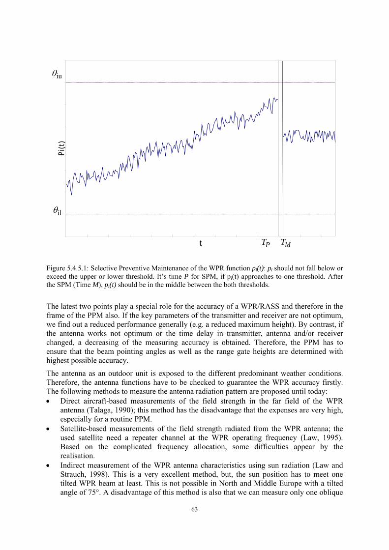
63

t

Pi(t)

ilθ

iuθ

PT MT

Figure 5.4.5.1: Selective Preventive Maintenance of the WPR function pi(t): pi should not fall below or exceed the upper or lower threshold. It�s time P for SPM, if pi(t) approaches to one threshold. After the SPM (Time M), pi(t) should be in the middle between the both thresholds.

The latest two points play a special role for the accuracy of a WPR/RASS and therefore in the frame of the PPM also. If the key parameters of the transmitter and receiver are not optimum, we find out a reduced performance generally (e.g. a reduced maximum height). By contrast, if the antenna works not optimum or the time delay in transmitter, antenna and/or receiver changed, a decreasing of the measuring accuracy is obtained. Therefore, the PPM has to ensure that the beam pointing angles as well as the range gate heights are determined with highest possible accuracy.

The antenna as an outdoor unit is exposed to the different predominant weather conditions. Therefore, the antenna functions have to be checked to guarantee the WPR accuracy firstly. The following methods to measure the antenna radiation pattern are proposed until today: • Direct aircraft-based measurements of the field strength in the far field of the WPR

antenna (Talaga, 1990); this method has the disadvantage that the expenses are very high, especially for a routine PPM.

• Satellite-based measurements of the field strength radiated from the WPR antenna; the used satellite need a repeater channel at the WPR operating frequency (Law, 1995). Based on the complicated frequency allocation, some difficulties appear by the realisation.

• Indirect measurement of the WPR antenna characteristics using sun radiation (Law and Strauch, 1998). This is a very excellent method, but, the sun position has to meet one tilted WPR beam at least. This is not possible in North and Middle Europe with a tilted angle of 75°. A disadvantage of this method is also that we can measure only one oblique

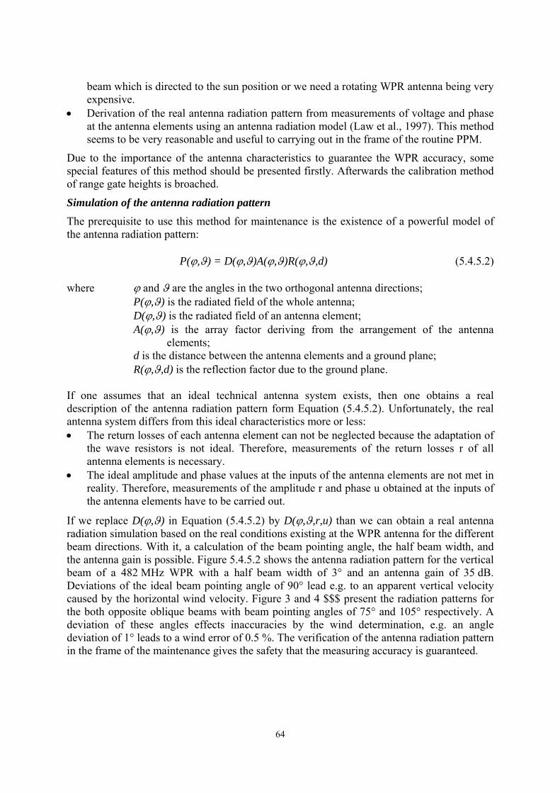
64

beam which is directed to the sun position or we need a rotating WPR antenna being very expensive.

• Derivation of the real antenna radiation pattern from measurements of voltage and phase at the antenna elements using an antenna radiation model (Law et al., 1997). This method seems to be very reasonable and useful to carrying out in the frame of the routine PPM.

Due to the importance of the antenna characteristics to guarantee the WPR accuracy, some special features of this method should be presented firstly. Afterwards the calibration method of range gate heights is broached.

Simulation of the antenna radiation pattern

The prerequisite to use this method for maintenance is the existence of a powerful model of the antenna radiation pattern: P(ϕ,ϑ) = D(ϕ,ϑ)A(ϕ,ϑ)R(ϕ,ϑ,d) (5.4.5.2) where ϕ and ϑ are the angles in the two orthogonal antenna directions; P(ϕ,ϑ) is the radiated field of the whole antenna; D(ϕ,ϑ) is the radiated field of an antenna element; A(ϕ,ϑ) is the array factor deriving from the arrangement of the antenna elements; d is the distance between the antenna elements and a ground plane; R(ϕ,ϑ,d) is the reflection factor due to the ground plane. If one assumes that an ideal technical antenna system exists, then one obtains a real description of the antenna radiation pattern form Equation (5.4.5.2). Unfortunately, the real antenna system differs from this ideal characteristics more or less: • The return losses of each antenna element can not be neglected because the adaptation of

the wave resistors is not ideal. Therefore, measurements of the return losses r of all antenna elements is necessary.

• The ideal amplitude and phase values at the inputs of the antenna elements are not met in reality. Therefore, measurements of the amplitude r and phase u obtained at the inputs of the antenna elements have to be carried out.

If we replace D(ϕ,ϑ) in Equation (5.4.5.2) by D(ϕ,ϑ,r,u) than we can obtain a real antenna radiation simulation based on the real conditions existing at the WPR antenna for the different beam directions. With it, a calculation of the beam pointing angle, the half beam width, and the antenna gain is possible. Figure 5.4.5.2 shows the antenna radiation pattern for the vertical beam of a 482 MHz WPR with a half beam width of 3° and an antenna gain of 35 dB. Deviations of the ideal beam pointing angle of 90° lead e.g. to an apparent vertical velocity caused by the horizontal wind velocity. Figure 3 and 4 $$$ present the radiation patterns for the both opposite oblique beams with beam pointing angles of 75° and 105° respectively. A deviation of these angles effects inaccuracies by the wind determination, e.g. an angle deviation of 1° leads to a wind error of 0.5 %. The verification of the antenna radiation pattern in the frame of the maintenance gives the safety that the measuring accuracy is guaranteed.

65

Figure 5.4.5.2: Antenna radiation pattern of the vertical beam of a 482 MHz WPR based on an antenna model and above described antenna measurements; the figure shows the dependence of the gain in dB from the elevation angle for a constant azimuth.

Figure 5.4.5.3: Antenna radiation pattern of the oblique beam X-Minus of a 482 MHz WPR; the beam pointing angle is 75°.

66

Figure5.4.5.4: Antenna radiation pattern of the oblique beam X-Plus of the 482 MHz WPR; the beam pointing angle is 105°.

Calibration of range gate heights and range resolution

An exact determination of range gate heights and range resolution is necessary to guarantee the accuracy of WPR/RASS measurements. Therefore, an adjustment of these parameters has to be a part of the PPM. A range gate height is determined by the transit time in the atmosphere mainly but also by the delay time within the transmitter, receiver, and antenna. The essence of this kind of calibration is an exact determination of the delay time ∆tWPR within the WPR units.

Van de Kamp (1995) proposed a method to calibrate the distance of certain range gates using a delay line with a constant delay time ∆tC. The delay line simulates a target at a specific height of the atmosphere. Because ∆tC is known and the sum of ∆tC and ∆tWPR can be measured, a determination of the delay time ∆tWPR is possible. This method seems to be just right for PPM.

4.6. Expenses

In contrast to the monitoring of processed and transmitted data, the realisation of the monitoring of technical parameters needs certain hardware expenses. Therefore, we have to ask how many technical parameters and functions should be watched. One can answer simply that so much technical parameters and functions of a WPR/RASS have to be acquire that a sufficient assessment of the whole system function is possible. In contrast to the technical parameters, the monitoring of processed and transmitted data requires special software tools having a small size compared to the WPR/RASS processing software. The costs necessary for the monitoring of the whole system are restricted due to economical aspects and should not exceed about 5 % of the total cost of a WPR/RASS.

The running costs for the maintenance of a WPR/RASS depend on the system quality as well as on the number of wearing parts within the system. The replacement rate should be as low

67

as possible and the wearing parts should have a life time as long as possible respectively. Additionally, the number of wearing parts within a WPR/RASS has to be as small as possible.

The maintenance of WPR/RASS requires specialists with practical experiences on radar technology and high frequency technique. The maintenance staff has to trained on the special field of the WPR/RASS processing software. A maintenance staff of about two to four people should be able to carried out the service and maintenance of a network of some WPR/RASS.

5. Operational characteristics

5.1. Characteristics of an operational system

As COST 76 progressed there were significant discussion about the availability and quality of measurements required for an operational system. There was clearly no simple answer, since the requirements of systems deployed specifically for aviation operations at airports were not the same as systems deployed for general upper air network operations or those considered satisfactory for scientific research. Thus, most national groups preparing for upper air network operations felt that 90 per cent availability would be adequate. This was as long as the missing data were randomly scattered throughout the operational period, rather than the result of failure to operate for a continuous block of 10 per cent of the monitoring period.

Although some newer designs were completed during COST 76, most of the systems in use had been conceived at an earlier stage. This raises the question of whether the initial designs, usually optimised for a research purpose, were necessarily the best solution for operations. For instance, it is clear that some current 1 GHz designs have not been optimised for ease of long term maintenance, since they contain large numbers of relays that have to be replaced at regular intervals. These relays allow the use of a single small portable antenna with electronic beam steering for research purposes. However, a larger system with a number of antennas in fixed positions might be much more suitable for remote sites, where maintenance visits may only be possible once or twice a year.

Operational profilers at 1 GHz in the UK will be operated in future with either microwave radiometers or GPS total water vapour sensors. The signal from the profilers will be used to identify upper cloud layers and also to provide indication of significant layered structures in water vapour and temperature. In an ideal world, the 1 GHz profiler would thus be able to reliably sense upper cloud up to heights of about 10 km, whilst 6 to 8 km appears to be the current height limit. Total water vapour measurements primarily provide information on the water content between 0 and 4 km in UK conditions. Thus, lower troposphere profilers operated with total water vapour measurements would ideally measure return signals up to heights of 3 to 4 km at about 100 m vertical resolution for most of the time. The current upper limit is between 1.5 and 2.5 km. Further work is required to see whether the increase in overall sensitivity of the radar could be achieved without excessive increase in capital costs.

In contrast, the prototype operational profilers at 50 MHz seem to have aimed for data coverage to too high a level, expecting to be used as a full replacement for a radiosonde. In practice, full replacement of radiosonde observation coverage is not required by most potential profiler operators, so the economics of antenna size suggests that accepting a lower maximum height may lead to a lower cost and more systems being deployed.

The rate of change in the profiler hardware designs is low, since the relatively low number of systems that are currently being sold do not justify a high rate of change. In the American

68

network, the antenna designs have been revised to improve ease of maintenance, but large-scale radical changes to the systems have yet to be implemented, including the changeover of operating frequency requested by the radiofrequency regulators.

The companies involved in manufacturing profiler systems are not making large profits from this activity. In one European country, the company involved in the manufacture of an operational prototype at 482 MHz became bankrupt (for reasons other than problems with the profiler business) causing significant losses to its partner in this development programme. Thus, it is clearly very important that users of operational profilers collaborate together in providing relatively uniform specifications for the systems, so that the manufacturers are able to concentrate on optimising a limited number of designs.

As with the targets for operational performance, it was difficult to obtain a consensus within COST 76 on the quality of available operational software. Thus, the relative significance of various developments to address existing problems was also difficult to assess. For instance, most of the profilers operating for long periods and contributing to CWINDE were capable of achieving close to 90 per cent data availability, even given known software deficiencies. Thus, bird migration introduces errors occasionally at many sites in Europe, but rarely on the scale encountered by the operational network in North America. In the UK, the improved operational software supplied in recent years rejects more winds in rain than in the earlier versions. The rejection criteria do not appear properly matched to the conditions actually preventing reliable wind measurements in the UK. So on occasions poor winds are reported, whilst on other days winds are rejected when valid observations could be produced. However, the percentage data availability problem is not as high as 10 per cent in a month�s monitoring.

Thus, whilst certain aspects of data processing can be improved by various techniques, discussed in other sections of this report, the testing of this software needs to be extensive to demonstrate benefit in all the operational conditions encountered year by year. Thus, some European countries have chosen to purchase new operational systems, relying on the current basic software with its know limitations. This is instead of immediately implementing newer versions of more complex software. There is concern that the complexity of some proposed solutions may make identifying the source of basic measurement errors through instrument malfunction more difficult.

5.2. An example of remote operation of wind profilers

In the past, there were few requirements for prolonged remote operation of wind profiler systems. Most installations were based at a site, which had technical staff readily available to investigate any problems. In addition there was little requirement to provide data in real time. However with the realisation of the requirement to supply real-time wind measurements to NWP models, the demands on reliable remote operation interfaces and robust communications for profilers became an important issue.

As an example, the Met Office (UK) has operated three 1 GHz systems for more than 2 years. A primary aim of this pilot network, see Figure 5.5.2.1, was to assess the reliability of these systems at unmanned sites and their capabilities in providing real-time data to the network hub. This section summarises the outcome of this project.

Of the three boundary layer systems, one was installed at Camborne (a 24-hour manned site), one at Dunkeswell (an unmanned site with a local caretaker) and the third at Pendine (an unmanned site requiring a 4-hour drive to visit). The system at Pendine has subsequently been moved to a manned forecast site at Wattisham as part of the operational upper air network.

69

Figure 5.5.2.1: UK pilot wind profiler network and Doppler weather radar network in the south of the British Isles. Bracknell is the communications hub.

All sites were required to send wind data each hour to the network center at Bracknell. For Pendine and Dunkeswell all performance monitoring, configuration changes and data archiving was actioned through the remote access software. The network was set-up using standard telecommunications lines and the wind profilers were operated using the Radian LAPXM software working on Microsoft Windows NT. Regular monitoring of the data availability was performed during normal working hours and a summary was produced each month. Figure 5.5.2.2 shows the performance of the Pendine system from January 1999 through to when it was moved in January 2001. Initially there were problems with the wind profiler hardware causing a significant loss of data availability. These problems were resolved in July 1999 but real-time data loss was high due to problems with communications.

These problems were linked to when the profiler computer system was attempting to send the data files to the communications hub. On occasions this caused the communications to �lock�, and no more data were received at the hub until a complete reboot of the PC had been performed. In November 2000 this system was changed by using a computer at Bracknell to request the data files from the wind profiler computer. Once this happened, data availability at the hub increased to greater than 90 % on average.

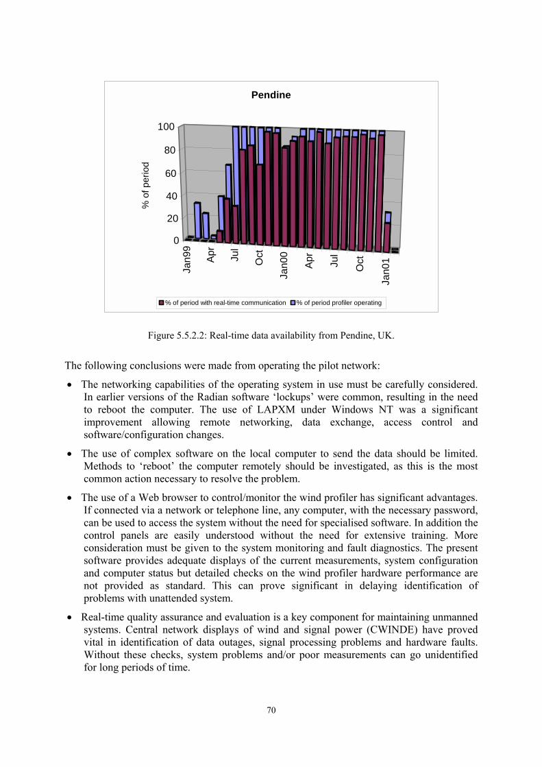
70

Jan9

9

Apr

Jul

Oct

Jan0

0

Apr

Jul

Oct

Jan0

1

0

20

40

60

80

100

% o

f per

iod

Pendine

% of period with real-time communication % of period profiler operating

Figure 5.5.2.2: Real-time data availability from Pendine, UK.

The following conclusions were made from operating the pilot network:

• The networking capabilities of the operating system in use must be carefully considered. In earlier versions of the Radian software �lockups� were common, resulting in the need to reboot the computer. The use of LAPXM under Windows NT was a significant improvement allowing remote networking, data exchange, access control and software/configuration changes.

• The use of complex software on the local computer to send the data should be limited. Methods to �reboot� the computer remotely should be investigated, as this is the most common action necessary to resolve the problem.

• The use of a Web browser to control/monitor the wind profiler has significant advantages. If connected via a network or telephone line, any computer, with the necessary password, can be used to access the system without the need for specialised software. In addition the control panels are easily understood without the need for extensive training. More consideration must be given to the system monitoring and fault diagnostics. The present software provides adequate displays of the current measurements, system configuration and computer status but detailed checks on the wind profiler hardware performance are not provided as standard. This can prove significant in delaying identification of problems with unattended system.

• Real-time quality assurance and evaluation is a key component for maintaining unmanned systems. Central network displays of wind and signal power (CWINDE) have proved vital in identification of data outages, signal processing problems and hardware faults. Without these checks, system problems and/or poor measurements can go unidentified for long periods of time.

71

6. Siting considerations

Siting

Proper siting of a wind profiling radar can help to considerably alleviate common problems connected with the operation of profilers such as: • clutter • electromagnetic interference • causing acoustic disturbances (this, of course, only in the case of a RASS system) • corrosion • lightning damage

Clutter Clutter can be caused either by airborne objects (aircraft, birds, insects) or by non-moving ground surfaces and/or buildings.

In order to minimise clutter from aircraft, the beams of a profiler should be oriented away from busy air routes. Because aircraft have an extremely large back scattering cross-section compared with the atmospheric eddies, it is not sufficient to only consider the main beam, but also the sidelobes of the antenna pattern must be included in such considerations.

Bird migration can be a significant problem for 400 and 1000 MHz wind profilers, hence, known migration paths should be avoided if possible in the same way as busy air routes.

Albeit to a lesser degree, also stationary obstacles seen by the side lobes may cause problems. In particular, this can become a problem when operating a profiler in a mountainous region. Again, proper orientation can greatly alleviate this problem.

On the other hand, when a 400 MHz profiler was operated within a city where practically all sidelobes intersected with the surrounding buildings, quality of wind data did not seem to be affected at all.

There are limits, both financial as well as technical ones, to the possible reduction of sidelobes in the primary (i.e., unshielded) radiation pattern of the antenna. Remaining sidelobes can be further reduced, e.g., by fences. These might either absorb the energy radiated in the sidelobes or reflect them in vertical direction. Also the above-mentioned buildings seem to have had the function of such a �fence�. Siting the antenna in a depression improves performance considerable, this again exclusively via an additional suppression of sidelobes. An experiment showed that siting a 400 MHz profiler in a gravel pit reduced sidelobes by 6 to 10 dB.

EMC considerations (ElectroMagnetic Compatibility)

There are basically two different problems connected with electromagnetic compatibility: (i) the profiler must be sufficiently protected from receiving signals within its receiver bandwidth from other sources, and (ii) the profiler must not emit signals which interfere with other communication (e.g. television) or location (e.g. radar) systems. When taking passive measures � such as proper siting or improving the antenna � to alleviate one of these two problems, the other one is always alleviated as well. (This is of course not the case for active measures such as increasing transmitter power.) For electromagnetic compatibility it is also important to consider possible mutual interference by unwanted emissions of wind profilers and other systems.

72

Potential EMC problems are rather specific for the different profiler families. The most important potential interfering systems include: ! 50 MHz: band I television systems (which, however, are gradually phased out),

communication systems. ! In at least one case, nearby power lines seriously disturbed the operation of a 50 MHz

system. It seemed that this was due to the fact that the power cables were not fixed firmly to the supporting insulators, but were allowed to slide when they contracted or expanded because of temperature changes.

! 400 MHz: band IV television systems ! 1000 MHz: air route surveillance radars (ARSR)

Wherever possible, a maximum frequency separation as well as a maximum distance separation should be sought. While it is generally difficult to postulate rules, experience as well as theoretical considerations show that 400 MHz profilers can operate within a television channel, provided a separation distance of about 40 km from the limit of the servicing area of the TV transmitter in question is maintained. Since TV transmitters radiate horizontally, while wind profilers transmit vertically, maximal side lobe suppression is, once more, an effective measure for preventing problems.

Co-channel operation with ARSR has not been investigated; however, experiments were carried out where the spectrum of a 1260 MHz ARSR partially overlapped with that of a 1290 MHz profiler. A separation of 8 km proved to be sufficient to prevent the radar from interfering with the profiler. (Given the huge power of the ARSR, the problem of the profiler interfering with the radar is not an issue.)

Some operators of Earth exploration satellites using synthetic aperture radar (SARs) have claimed to suffer from interference caused by wind profilers. However, there is no evidence � neither experimental nor theoretical � that a wind profiler has interfered with a SAR system. It should be remembered that the power in the very narrow main beam of a profiler is about 20 dB less than the isotropically radiated power of an ARSR, and both are operated in the same frequency region.

For completeness it should be mentioned that original concerns about interference with location systems (GPS, 1227.60 MHz and 1575.42 MHz) and/or Search-and-Rescue satellites (COSPAR/SARSAT, 406.05 MHz) are not an issue any more; these problems were solved by assigning operating frequencies for profilers sufficiently separated from the operating frequencies of said systems (see also Section 5.1). At any rate, different siting cannot alleviate interference problems with any air- or spaceborne system.

In summary, for alleviating any of the EMC problems, proper distance and/or frequency separation, an optimised orientation of the inclined beams, plus a very �clean� radiation pattern are the most effective means. The latter can be improved by either �artificial� (fence) or �natural� (depression) shielding.

Acoustic disturbance In the case of RASS, acoustic noise is an issue. While environmental noise from highways and/or aircraft is not disturbing RASS operation, the sound source used in the RASS can be a significant environmental problem. This problem is greater for fixed or swept frequencies, it is smaller for systems that employ random switching between acoustic frequencies.

Measures for reducing unwanted sound immissions include primarily a proper distance separation and shielding of the sound source. Of particular concern is night time operation:

73

Firstly, the lower background noise increases the subjective impression of the RASS sound source becoming more intense, secondly, night-time inversions might actually increase sound level at surface level due to acoustic ducting. Obviously, these problems are more significant in residential areas than in industrial regions.

Corrosion Experience has shown that salt spray at sites near the sea causes significant corrosion on the profiler antenna and on any exposed parts such as phasing network and switching elements. Hence, sites should be chosen where salt spraying is minimal, if it cannot be avoided completely, additional protection becomes mandatory.

Lightning For obvious reasons, lightning can cause severe damage to a wind profiler. Lightning protection should be carefully considered when setting up any system.

7. Data coding

7.1. Introduction

For international data exchange and dissemination of observations, the table-driven code FM-94 �BUFR“ (Binary Universal Form for the Representation of meteorological data, [WMO, 1994]) is the standard code format of the World Meteorological Organisation (WMO). It has been approved for operational use in 1988 and is recommended for all present and future WMO applications. Recently, the ICT/DRC of WMO-CBS (Commission for Basic Systems) had been tasked by CBS Ext.98 with developing BUFR Common Data Templates for all traditional alphanumeric code forms (WMO, 2000).

Data coding via BUFR has been used mainly, so far, for satellite, aircraft and wind profiler (North America) observations, but also for tropical cyclone information and for archiving of all types of observational data. BUFR allows universal, efficient, and compact data representation and transmission of data messages via the GTS of almost any measuring equipment or observation. It offers great advantages in comparison with the traditional alphanumeric codes. The main features of BUFR are self-description, flexibility and expandability, which are fundamental in times of fast scientific and technical evolution. In addition, BUFR-coded data are condensed (packed), and may include quality flags and associated values. Together with the other table-driven code of the WMO, �CREX“ (Character Form for the Representation and Exchange of Data), which should only be used if BUFR is not possible, it is the ideal tool for coding observations. BUFR can be easily expanded to satisfy all observational requirements, without deviating from WMO recommendations, even to answer national needs for specific domestic data exchange, as it is presently the case in many countries.

For the interchange of wind profiler radar (WPR) and RASS data between COST-76 member states, the COST-76 Management Committee identified the need to define and agree on an international acceptable standard code format and decided to use BUFR. A first working group, composed of experts from France, Germany and the United Kingdom was convened in Toulouse in March 1996 to agree on BUFR code tables for the Data Description Section (Section-3) of BUFR that would meet the needs of the WPR community in Europe (Engelbart et al., 1998). After some years of experience throughout the action COST-76, especially during the campaigns �COST Wind Initiative for a Network Demonstration in Europe”

74

(CWINDE-97 and CWINDE-99), some amendments arose to be necessary. This section will describe the idea of BUFR code tables as defined by COST-76 and gives explanations on these, where some reference is made to the Final Report of the WMO-CBS OPAG on Information and Services concerning their �Meeting of the Implementation/ Co-ordination Team on Data Representation and Codes” (WMO, 2000).

7.2. Background

A general problem concerning data dissemination from measuring equipment which is still in development is the question which information to disseminate. After years of futile proposals throughout the COST-74 action there is now, since 1996, a reasonable working compilation of descriptors for WPR/RASS. It divides all interesting data in an user-oriented raw-data and a processed-data message as well as a general site/system information header respectively.

The idea of transmitting either processed or raw data takes into account all possible types of profiler systems as well as data processing organisations. This is a major difference compared with earlier solutions of WPR data dissemination using BUFR as it is used e.g. by the NOAA Profiler Network (NPN) in the United States. Nevertheless, the European structure of WPR data transmission via BUFR has been discussed and agreed with the NPN before realisation. The reason for not adopting the NPN structure and sequences for BUFR simply base on the non-homogeneous network of WPR in Europe. Therefore in Europe, and similarly in all regions having various profiler types and/or network configurations, a different and more universal approach had to be chosen, as for instance not every profiler site allows to process the data locally. The other idea of the European approach made by COST-76 is that it serves two main user groups, i.e. the end-users (e.g. forecasters), who are mainly interested in quality-controlled end products, and the scientific users, who are interested in practically all information available.

Hence, given the potentially large quantities of data that WPR systems can generate, meteorological information has been divided into two separate message formats, i.e. a standard product format (processed data) and the raw data format. The latter includes measurements such as backscattered power, radial velocities and spectral width. This separation will enable meteorological database managers to archive only the meteorologically important parameters and on the other hand allowing specialised access to raw data for research purposes as and when required.

7.3. Some remarks to the general structure of BUFR

Similar to an alphanumeric code like e.g. the FM-12 SYNOP, the WMO standard code for land surface observations, in a table-driven code there are also position rules. However, those apply only to the frame, i.e. to the shape of the »container« rather than to the content itself. This means, the presence of a datum is described in the in the message itself: It is the self description feature. Thus, there will be a section at the beginning of a BUFR message, which defines what data are transmitted in it. That section will in fact contain pointers towards elements in predefined and internationally agreed tables which are store in the official WMO Manual on Codes (see references). Once this section, being called the Data Description Section is read, the following part of the message containing the data, the Data Section can be understood. Indeed, the characteristics of the parameters to be transmitted must already be defined in the tables of the WMO manual. The �pointers� in the Data Description Section are

75

in fact numbers called �descriptors�, which correspond to entries in the BUFR tables, published in the WMO Manual on Codes (WMO, 1995).

The layout of a BUFR message consists of six different sections which are defined as follows (e.g. WMO, 1994): Section-0 (Indicator Section) simply consists of the word �BUFR�. Section-1, the identification section, particularly contains the length of this section, generally expressed in octets (bytes), and some identification of the message itself. Section-2 then is an optional section that can be used to transmit any information or parameters for national purpose, i.e. it is designed for local use by automatic data processing (ADP) centres and is somehow the equivalent of national groups in traditional alphanumeric codes. Section-3, the Data Description Section, consists again of the length of the section, the number of data subsets, type of BUFR message flag and a collection of descriptors which define the form and content of individual data elements which will follow in Section-4, being the Data Section, which contains the data in binary format. The final Section-5 (End Section) is again very short and terminates a BUFR message by the four bytes �7777�.

In BUFR the parameters are simply listed as required by the user of the codes, e.g. a WPR/RASS operator. The datum are laid out one after the other and an item, i.e. the data value of a parameter to be transmitted in a message, will be translated in a set of bits in BUFR.

When there is a requirement for transmission of new parameters or new data types like for instance WPR and RASS measurements or quantities derived from these instruments, new elements are simply added to the WMO BUFR Tables after submission and approval by the WMO Commission on Basic Systems (CBS). Table-driven codes can transmit an infinity of information. A definition of new »codes« as such is no more necessary. The expansion of tables is sufficient. An edition number is associated for every new table version. This information is transmitted in the message itself (Identification Section-2) and enables the treatment of old archived data.

BUFR tables define how the parameters (the elements) shall be coded as data items in a message. In the WMO Manual on Codes four tables (A-D) define BUFR coding. Table-A defines the data category, Table-B contains the list of elements (parameters) and describes the format of the data following in the Data Section-4. In case of the need to change the format (e.g. resolution) of data to be transmitted, BUFR offers some operators, for example to change any of the format parameters (scale, reference value, data width) or other things defined in Table-B. Operators like these are described in Table-C. As BUFR allows to define groups of data items being always transmitted altogether, Table-D finally contains a list of currently defined groups of descriptors, the so-called Common Sequence Descriptors (sequences). Using these sequences in the Data Description Section-3 avoids the need to repeat the individual element descriptors of the sequence each time when they are used, i.e. in Section-3, only the common sequence descriptor will be listed.

BUFR also offers condensation, meaning data will require less resources for transmission and stocking. Condensation or packing is performed by an algorithm within the code regulations. BUFR also permits the transmission of associated data, like flags, quality bytes, etc. with the original observation data. However, the big disadvantage is that human cannot read BUFR directly. BUFR processing does assume the availability of well-designed computer programs, i.e. decoder and encoder for the reverse, that are capable of parsing the descriptors, matching them to a bit stream of data and extracting the numbers from the bit stream, and finally reformatting the numbers in a way suitable for subsequent calculations.

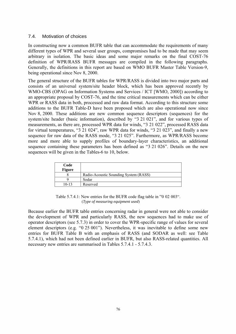
76

7.4. Motivation of choices

In constructing now a common BUFR table that can accommodate the requirements of many different types of WPR and several user groups, compromises had to be made that may seem arbitrary in isolation. The basic ideas and some major remarks on the final COST-76 definition of WPR/RASS BUFR messages are compiled in the following paragraphs. Generally, the definitions in this report are based on WMO BUFR Master Table Version-9, being operational since Nov 8, 2000.

The general structure of the BUFR tables for WPR/RASS is divided into two major parts and consists of an universal system/site header block, which has been approved recently by WMO-CBS (OPAG on Information Systems and Services / ICT [WMO, 2000]) according to an appropriate proposal by COST-76, and the time critical measurements which can be either WPR or RASS data in both, processed and raw data format. According to this structure some additions to the BUFR Table-D have been proposed which are also operational now since Nov 8, 2000. These additions are new common sequence descriptors (sequences) for the system/site header (basic information), described by �3 21 021�, and for various types of measurements, as there are, processed WPR data for winds, �3 21 022�, processed RASS data for virtual temperatures, �3 21 024�, raw WPR data for winds, �3 21 023�, and finally a new sequence for raw data of the RASS mode, �3 21 025�. Furthermore, as WPR/RASS become more and more able to supply profiles of boundary-layer characteristics, an additional sequence containing these parameters has been defined as �3 21 026�. Details on the new sequences will be given in the Tables-6 to 10, below.

Code

Figure

8 Radio-Acoustic Sounding System (RASS) 9 Sodar

10-13 Reserved

Table 5.7.4.1: New entries for the BUFR code flag table in �0 02 003�. (Type of measuring equipment used)

Because earlier the BUFR table entries concerning radar in general were not able to consider the development of WPR and particularly RASS, the new sequences had to make use of operator descriptors (see 5.7.3) in order to cover the WPR-specific range of values for several element descriptors (e.g. �0 25 001�). Nevertheless, it was inevitable to define some new entries for BUFR Table B with an emphasis of RASS (and SODAR as well: see Table 5.7.4.1), which had not been defined earlier in BUFR, but also RASS-related quantities. All necessary new entries are summarised in Tables 5.7.4.1 - 5.7.4.3.

77

TABLE

REFERENCE F X Y

ELEMENT NAME

UNIT

SCALE

REFERENCE

VALUE

DATA WIDTH (BITS)

0 21 091 Radar signal Doppler spectrum 0th moment DB 0 -100 8

0 21 092 RASS signal Doppler spectrum 0th moment, referring to RASS signal

DB 0 -100 8

Table 5.7.4.2: New entries for BUFR Table B in Class-21 (Radar data).

TABLE REFERENCE F X Y

ELEMENT NAME

UNIT

SCALE

REFERENCE

VALUE

DATA WIDTH (BITS)

0 25 091 Structure constant of the refraction index (cn2) DB 3 -18192 13

0 25 092 Acoustic propagation velocity m s-1 2 28�000 14

0 25 093 RASS computation correction Flag table 0 0 8

Table 5.7.4.3: New entries for BUFR Table B in Class-25 (Processing information).

Bit No. 1 No correction 2 Vertical velocity correction 3-6 Reserved 7 All corrections All 8 Missing value

Table 5.7.4.4: New definition of the BUFR flag table �0 25 093� (RASS computation correction).

Because the last entry in Table 5.7.4.3 refers to a flag table, this table had to be defined too (see Table 5.7.4.4).

As WPRs are able to derive information from two or more different pulse widths (measuring modes) quasi-simultaneously, data from all different modes may be transmitted easily by a compilation of each mode�s data set into separate BUFR messages (files). In order to distinguish arriving BUFR messages directly, i.e. without the need to decode them first, the WPR BUFR messages of the CWINDE WPR Network (CPN) can be identified by two different ways, where both refer to arrangements of, or between local ADP centres, i.e. these are no general, WMO-wide methods: Method-1 makes use of Octet-10 in BUFR Section-1. This octet allows to define data category sub-types which have been defined for the CPN according to Table 5.7.4.5.

The second method, which has to be used simultaneously within the CPN employs the human-readable bytes starting from Octet-18 in Section-1, containing an ASCII name of the BUFR message. This name, being written in uppercase letters, unambiguously defines not only the disseminating radar site, the measuring mode in case of more than one, and the type of message (wind profile or RASS, processed or raw data) but also the time of observation. The idea of naming simply is to allow any required selection of messages for archiving or data extraction without decoding.

78

Code Figure

0 not in use 1 processed profiler data: Winds 2 Raw profiler data: Winds 3 Processed profiler data: RASS temperatures 4 Raw profiler data: RASS temperatures

Table 5.7.4.5: CPN definitions for the data category sub-type, described by Octet-10 in BUFR Section-1.

The inclusion of the filename in Section-1 of BUFR is in principle optional. Because the application of this naming influences the total length of Section-1, this length has to be described by Octet 1-3. Generally, within the framework of the CWINDE projects and when transmitting data to the UKMO for display at the CWINDE WWW pages, the inclusion of a filename is mandatory and the names of the BUFR message files must conform to the following structure:

File name (for Section-1 of BUFR): IIISS_MMDDhhmm.PPP

where: III = Three letter radar identifier

SS = Two letter profile type identifier, defined as follows WPR = Wind Profile RS = RASS temperature profile AD = Additional <Boundary Layer> Data MM = Month DD = Day of month

hh = Time of measurement: Hours (end of averaging interval) mm = Time of measurement: Minutes (end of averaging interval) PPP = Three letter data type identifier:

PRO = Processed data (winds or virtual temperatures) RAW = RAW data (SNR, radial velocities, spectral widths, etc.)

79

Currently defined radar identifiers within the CPN are:

Radar site Identifier Radar site Identifier Aberystwyth ABW Lannemezan LAN Aberystwyth BLR (low) AB1 L�Aquila LAQ Aberystwyth BLR (high) AB2 Lindenberg (1290 MHz) LB1 Andenes AND Lindenberg (482 MHz, low) LB2 Bilbao BIL Lindenberg (482 MHz, high) LB3 Brest BRE La Ferté Vidame LFV Cabauw (high) CAB Nice (high) NI1 Cabauw (low) CB2 Nice (low) NI2 Camborne (high) CAM Payerne (high) PAY Camborne (low) CM2 Payerne (low) PY2 Clermont Ferrand CLF Pendine (high) PEN Dunkeswell (high) DUN Pendine (low) PN2 Dunkeswell (low) DN2 Rome ROM Hamburg (Itzehoe) HAM Salzburg SZB Innsbruck INN Toulouse TOU Karlsruhe KAR Vagar VGA Kiruna KIR Vienna VIE

Table 5.7.4.6: Currently defined radar identifiers within the CPN.

Additional three-letter station identifiers have to be negotiated between any new radar site wishing to display data on the CWINDE web pages being located at �http://www.meto.gov.uk/sec5/CWINDED/cwinde99/cwindemape.html� and the database manager at Bracknell (see also Section 5.8).

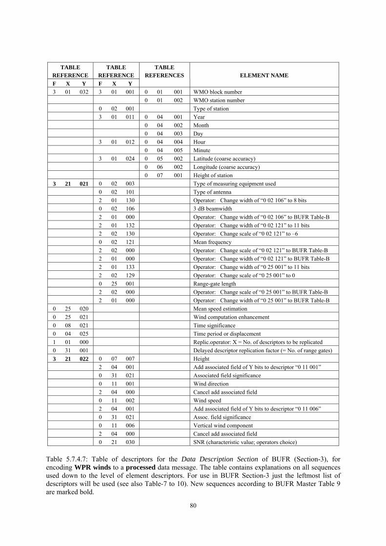
80

TABLE

REFERENCE TABLE

REFERENCE TABLE

REFERENCES

ELEMENT NAME F X Y F X Y 3 01 032 3 01 001 0 01 001 WMO block number 0 01 002 WMO station number 0 02 001 Type of station 3 01 011 0 04 001 Year 0 04 002 Month 0 04 003 Day 3 01 012 0 04 004 Hour 0 04 005 Minute 3 01 024 0 05 002 Latitude (coarse accuracy) 0 06 002 Longitude (coarse accuracy) 0 07 001 Height of station 3 21 021 0 02 003 Type of measuring equipment used 0 02 101 Type of antenna 2 01 130 Operator: Change width of �0 02 106� to 8 bits 0 02 106 3 dB beamwidth 2 01 000 Operator: Change width of �0 02 106� to BUFR Table-B 2 01 132 Operator: Change width of �0 02 121� to 11 bits 2 02 130 Operator: Change scale of �0 02 121� to �6 0 02 121 Mean frequency 2 02 000 Operator: Change scale of �0 02 121� to BUFR Table-B 2 01 000 Operator: Change width of �0 02 121� to BUFR Table-B 2 01 133 Operator: Change width of �0 25 001� to 11 bits 2 02 129 Operator: Change scale of �0 25 001� to 0 0 25 001 Range-gate length 2 02 000 Operator: Change scale of �0 25 001� to BUFR Table-B 2 01 000 Operator: Change width of �0 25 001� to BUFR Table-B 0 25 020 Mean speed estimation 0 25 021 Wind computation enhancement 0 08 021 Time significance 0 04 025 Time period or displacement 1 01 000 Replic.operator: X = No. of descriptors to be replicated 0 31 001 Delayed descriptor replication factor (= No. of range gates) 3 21 022 0 07 007 Height 2 04 001 Add associated field of Y bits to descriptor �0 11 001� 0 31 021 Associated field significance 0 11 001 Wind direction 2 04 000 Cancel add associated field 0 11 002 Wind speed 2 04 001 Add associated field of Y bits to descriptor �0 11 006� 0 31 021 Assoc. field significance 0 11 006 Vertical wind component 2 04 000 Cancel add associated field 0 21 030 SNR (characteristic value; operators choice)

Table 5.7.4.7: Table of descriptors for the Data Description Section of BUFR (Section-3), for encoding WPR winds to a processed data message. The table contains explanations on all sequences used down to the level of element descriptors. For use in BUFR Section-3 just the leftmost list of descriptors will be used (see also Table-7 to 10). New sequences according to BUFR Master Table 9 are marked bold.

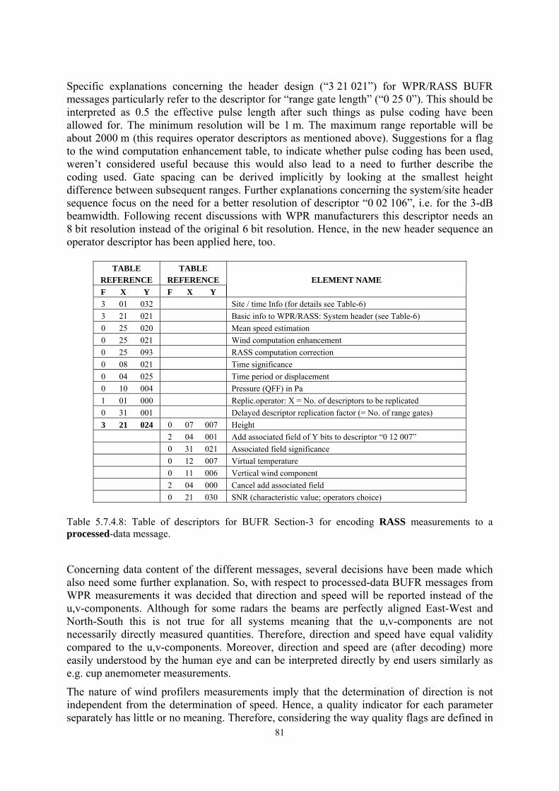
81

Specific explanations concerning the header design (�3 21 021�) for WPR/RASS BUFR messages particularly refer to the descriptor for �range gate length� (�0 25 0�). This should be interpreted as 0.5 the effective pulse length after such things as pulse coding have been allowed for. The minimum resolution will be 1 m. The maximum range reportable will be about 2000 m (this requires operator descriptors as mentioned above). Suggestions for a flag to the wind computation enhancement table, to indicate whether pulse coding has been used, weren�t considered useful because this would also lead to a need to further describe the coding used. Gate spacing can be derived implicitly by looking at the smallest height difference between subsequent ranges. Further explanations concerning the system/site header sequence focus on the need for a better resolution of descriptor �0 02 106�, i.e. for the 3-dB beamwidth. Following recent discussions with WPR manufacturers this descriptor needs an 8 bit resolution instead of the original 6 bit resolution. Hence, in the new header sequence an operator descriptor has been applied here, too.

TABLE REFERENCE

TABLE REFERENCE

ELEMENT NAME

F X Y F X Y 3 01 032 Site / time Info (for details see Table-6) 3 21 021 Basic info to WPR/RASS: System header (see Table-6) 0 25 020 Mean speed estimation 0 25 021 Wind computation enhancement 0 25 093 RASS computation correction 0 08 021 Time significance 0 04 025 Time period or displacement 0 10 004 Pressure (QFF) in Pa 1 01 000 Replic.operator: X = No. of descriptors to be replicated 0 31 001 Delayed descriptor replication factor (= No. of range gates) 3 21 024 0 07 007 Height 2 04 001 Add associated field of Y bits to descriptor �0 12 007� 0 31 021 Associated field significance 0 12 007 Virtual temperature 0 11 006 Vertical wind component 2 04 000 Cancel add associated field 0 21 030 SNR (characteristic value; operators choice)

Table 5.7.4.8: Table of descriptors for BUFR Section-3 for encoding RASS measurements to a processed-data message.

Concerning data content of the different messages, several decisions have been made which also need some further explanation. So, with respect to processed-data BUFR messages from WPR measurements it was decided that direction and speed will be reported instead of the u,v-components. Although for some radars the beams are perfectly aligned East-West and North-South this is not true for all systems meaning that the u,v-components are not necessarily directly measured quantities. Therefore, direction and speed have equal validity compared to the u,v-components. Moreover, direction and speed are (after decoding) more easily understood by the human eye and can be interpreted directly by end users similarly as e.g. cup anemometer measurements.

The nature of wind profilers measurements imply that the determination of direction is not independent from the determination of speed. Hence, a quality indicator for each parameter separately has little or no meaning. Therefore, considering the way quality flags are defined in

82

BUFR code and although referring to both quantities, a single one bit flag is assigned only to wind direction. Vertical velocity may or may not be an independent measurement depending on a given radar configuration, so it's quality flag may differ from that of the horizontal wind.

Because near-surface wind speed/direction (5 m or 10 m a.g.l.) is required for many applications and end-users, this parameter should be included as the first apparent WPR-data level in the processed data message for winds (sequence �3 21 022�). The same also holds for near-surface temperature with respect to the processed data message for RASS temperatures. In connection with the surface-level pressure, defined by the element descriptor �0 10 004�, which has been included into the system/site header sequence (�3 21 021�), this will moreover allow to calculate a potential temperature profile from RASS temperatures.

TABLE REFERENCE

TABLE REFERENCE

ELEMENT NAME

F X Y F X Y 3 01 032 Site / time Info (for details see Table-6) 3 21 021 Basic info to WPR/RASS: System header (see Table-6) 0 25 003 Number of integrated pulses (NCI) 0 25 020 Mean speed estimation 0 04 026 Time period or displacement (complete 3- or 5-beam cycle) 1 13 000 Replic.operator: X = No. of descriptors to be replicated 0 31 001 Delayed descriptor replication factor (= No. of profiler beams) 0 02 134 Antenna beam azimuth 0 02 135 Antenna elevation 1 01 000 Replic.operator: X = No. of descriptors to be replicated 0 31 001 Delayed descriptor replication factor (= No. of range gates) 3 21 023 0 07 007 Height

0 21 091 Radar signal Doppler spectrum 0th moment 0 21 030 SNR of the described beam 2 02 129 Operator: Change scale of �0 21 014� to 2 0 21 014 Doppler mean velocity (radial) 2 01 129 Operator: Change width of �0 21 017� to 9 bits 0 21 017 Doppler velocity spectral width 2 02 000 Change scale to BUFR Table-B 2 01 000 Change width to BUFR Table-B

Table 5.7.4.9: Table of descriptors for BUFR encoding of WPR winds to a raw data message.

Because signal-to-noise ratio (SNR) measurements are of increasing importance for data evaluation and interpretation, the processed data messages will include one (representative) value of this quantity per range gate (descriptor �0 21 030�). Since different conditions apply to each specific radar site and some sites have ground clutter or Fresnel reflection (VHF WPR) in the vertical beam, the choice of which SNR to put into the message will be left to each individual radar operator. Generally, SNR may give additional hints on data quality (e.g. scattering by birds or water droplets) as well as potentially supplying first-guess information on e.g. mixed-layer depth under clear-air conditions. Therefore, SNR will be included in the processed data message of WPR/RASS.

With respect to the raw data messages the following explanations should help to understand the respective choices: In order to make the raw data from all beams available the possibly variable number of beams transmitted is required. The format chosen for the raw messages

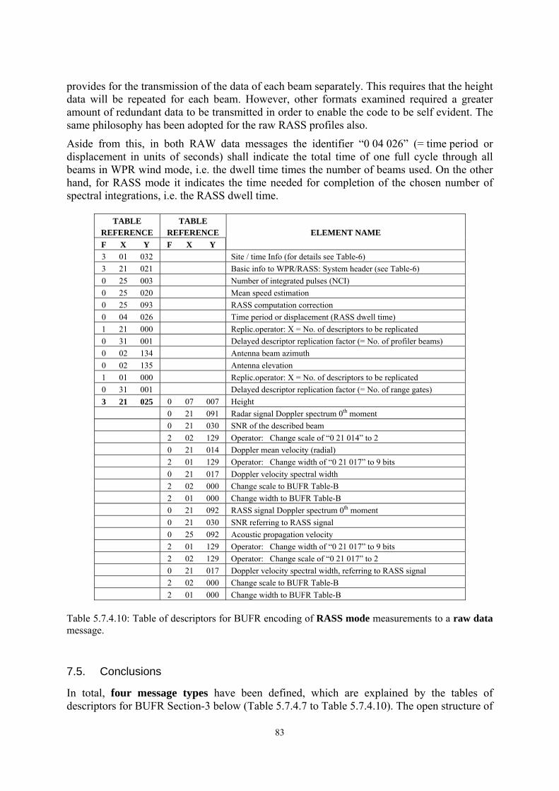
83

provides for the transmission of the data of each beam separately. This requires that the height data will be repeated for each beam. However, other formats examined required a greater amount of redundant data to be transmitted in order to enable the code to be self evident. The same philosophy has been adopted for the raw RASS profiles also.

Aside from this, in both RAW data messages the identifier �0 04 026� (= time period or displacement in units of seconds) shall indicate the total time of one full cycle through all beams in WPR wind mode, i.e. the dwell time times the number of beams used. On the other hand, for RASS mode it indicates the time needed for completion of the chosen number of spectral integrations, i.e. the RASS dwell time.

TABLE REFERENCE

TABLE REFERENCE

ELEMENT NAME

F X Y F X Y 3 01 032 Site / time Info (for details see Table-6) 3 21 021 Basic info to WPR/RASS: System header (see Table-6) 0 25 003 Number of integrated pulses (NCI) 0 25 020 Mean speed estimation 0 25 093 RASS computation correction 0 04 026 Time period or displacement (RASS dwell time) 1 21 000 Replic.operator: X = No. of descriptors to be replicated 0 31 001 Delayed descriptor replication factor (= No. of profiler beams) 0 02 134 Antenna beam azimuth 0 02 135 Antenna elevation 1 01 000 Replic.operator: X = No. of descriptors to be replicated 0 31 001 Delayed descriptor replication factor (= No. of range gates) 3 21 025 0 07 007 Height 0 21 091 Radar signal Doppler spectrum 0th moment 0 21 030 SNR of the described beam 2 02 129 Operator: Change scale of �0 21 014� to 2 0 21 014 Doppler mean velocity (radial) 2 01 129 Operator: Change width of �0 21 017� to 9 bits 0 21 017 Doppler velocity spectral width 2 02 000 Change scale to BUFR Table-B 2 01 000 Change width to BUFR Table-B 0 21 092 RASS signal Doppler spectrum 0th moment 0 21 030 SNR referring to RASS signal 0 25 092 Acoustic propagation velocity 2 01 129 Operator: Change width of �0 21 017� to 9 bits 2 02 129 Operator: Change scale of �0 21 017� to 2 0 21 017 Doppler velocity spectral width, referring to RASS signal 2 02 000 Change scale to BUFR Table-B 2 01 000 Change width to BUFR Table-B

Table 5.7.4.10: Table of descriptors for BUFR encoding of RASS mode measurements to a raw data message.

7.5. Conclusions

In total, four message types have been defined, which are explained by the tables of descriptors for BUFR Section-3 below (Table 5.7.4.7 to Table 5.7.4.10). The open structure of

84

the table format allows to define additional message types easily in case of significant progress in signal processing or data evaluation. As the derivation of additional products becomes more standardised, e.g. mixed-layer depth, turbulent fluxes, dissipation, and TKE (turbulent kinetic energy) for the boundary layer, or tropopause height in the free atmosphere, the described BUFR tables have a flexible design allowing to add new messages using the same header information as the existing messages. As an example for such an additional message a fifth table (Table 5.7.5.1) demonstrates the structure concerning the transmission of additional (boundary-layer) data from WPR/RASS.

TABLE REFERENCE

TABLE REFERENCE

ELEMENT NAME

F X Y F X Y 3 01 032 Site / time Info (for details see Table-6) 3 21 021 Basic info to WPR/RASS: System header (see Table-6) 0 25 020 Mean speed estimation 0 25 021 Wind computation enhancement 0 08 021 Time significance 0 04 025 Time period or displacement 2 04 001 Add associated field of Y bits to descriptor �0 13 006� 0 31 021 Associated field significance 0 13 006 Mixing height 2 04 000 Cancel add associated field 1 01 000 Replic.operator: X = No. of descriptors to be replicated 0 31 001 Delayed descriptor replication factor (= No. of range gates) 3 21 026 0 07 007 Height

2 04 001 Add associated field of Y bits to descriptor �0 12 007� 0 31 021 Associated field significance 0 12 007 Virtual temperature 0 25 091 Structure constant of the refraction index (cn²) (see Table-3) 0 11 071 Turbulent vertical momentum flux 0 11 072 Turbulent vertical buoyancy flux 0 11 073 Turbulent kinetic energy 0 11 074 Dissipation energy 2 04 000 Cancel add associated field

Table 5.7.5.1: Table of descriptors for BUFR encoding of boundary-layer parameters derived by WPR/RASS measurements.

8. Networking

An important part of the COST 76 project was to demonstrate that the wind profilers currently working in Europe could operate as part of a network and that this network could be sustained and supported over an agreed period. Thus in late 1996 the management committee agreed to initiate a campaign to network wind profiler measurements in real time within Europe (CWINDE � Cost Wind Initiative for a Network Demonstration in Europe). The networking issues to be addressed were not only connected with the wind profiler systems themselves but also the processing and displaying of the data in real time and the feedback of performance statistics to the operators. It was agreed that to set-up and support the necessary networking infrastructure (i.e. software, networking processes, advice etc.), a CWINDE Project Office

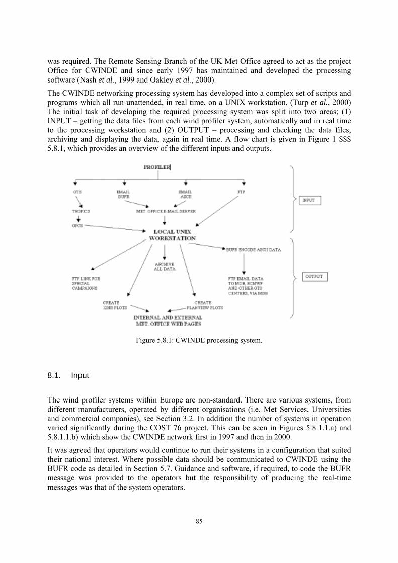
85

was required. The Remote Sensing Branch of the UK Met Office agreed to act as the project Office for CWINDE and since early 1997 has maintained and developed the processing software (Nash et al., 1999 and Oakley et al., 2000).

The CWINDE networking processing system has developed into a complex set of scripts and programs which all run unattended, in real time, on a UNIX workstation. (Turp et al., 2000) The initial task of developing the required processing system was split into two areas; (1) INPUT � getting the data files from each wind profiler system, automatically and in real time to the processing workstation and (2) OUTPUT � processing and checking the data files, archiving and displaying the data, again in real time. A flow chart is given in Figure 1 $$$ 5.8.1, which provides an overview of the different inputs and outputs.

Figure 5.8.1: CWINDE processing system.

8.1. Input

The wind profiler systems within Europe are non-standard. There are various systems, from different manufacturers, operated by different organisations (i.e. Met Services, Universities and commercial companies), see Section 3.2. In addition the number of systems in operation varied significantly during the COST 76 project. This can be seen in Figures 5.8.1.1.a) and 5.8.1.1.b) which show the CWINDE network first in 1997 and then in 2000.

It was agreed that operators would continue to run their systems in a configuration that suited their national interest. Where possible data should be communicated to CWINDE using the BUFR code as detailed in Section 5.7. Guidance and software, if required, to code the BUFR message was provided to the operators but the responsibility of producing the real-time messages was that of the system operators.

86

Figure 5.8.1.1.a): Wind profilers connected to CWINDE (Jan � Mar 1997).

Figure 5.8.1.1.b): Wind profilers considered for connection to CWINDE (March 2000).

Various communications methods were set-up to allow the transmission of messages from the different systems as follows: • Through the Global Telecommunication System (GTS) link to the UK Met Office. For

this routing the data must be BUFR encoded and contain the agreed WMO message header.

87

• BUFR encoded messages sent via Email to a dedicated CWINDE address. This required the files to be �uuencoded� before onward transmission.

• ASCII data messages, in a set format, sent via Email to a dedicated CWINDE address. Data then was coded into BUFR on the CWINDE workstation. This method was developed for wind profiler sites that did not have the necessary expertise/resource to implement the BUFR encoding software.

• An FTP (File Transfer Protocol) option, either by putting or getting the data, was set-up later in the campaign as an alternative and more reliable option to Email. This option was subject to access to an FTP site and security issues.

8.2. Real-time processing

A suite of programs has been developed to process any incoming data. All processing is carried out using UNIX workstations, currently using the HP-UX11 operating system. The data are processed in real time using a series of scheduled jobs continuously looking for incoming data sent via one of the following methods:

via GTS If the Wind Profiler station is linked to the Met Office via the GTS link then the messages may be sent directly to the Met. Office Central Data Network (CDN). The incoming messages must be BUFR encoded and contain a unique WMO header. The operational data messaging software then routes the messages to the following locations: a) Met. Office Operational Database � input into the Unified Model b) ECMWF (European Centre for Medium-range Weather Forecasts) c) Mainframe computer which forwards the messages to the Project Office.

via e-mail (BUFR encoded) The data must be BUFR encoded at the source and uuencoded before being transmitted via Email. A scheduled job then checks the mailbox every 15 minutes for incoming data. Any messages received are uudecoded, moved to the relevant directory and then the contents of the mailbox are deleted in preparation for new messages.

via e-mail (ASCII format)

The data must be in a set format with the profiler identification on the first line, followed by the date of the message and number of range gates on subsequent lines. A scheduled job then checks the mailbox every 15 minutes for incoming data. Any messages received are transferred to a file with the correct naming convention, BUFR encoded, moved to the relevant directory and then the contents of the mailbox are deleted in preparation for new messages.

via FTP The CWINDE workstation is able to access an FTP sites unattended, in real time. If the wind profiler system is able to transfer the BUFR files to a local FTP site then an FTP script can be initiate to copy the latest messages to the CWINDE system. This method of sending the data was set-up to overcome some of the shot comings of the Email option. It allows for data redundancy if either the Internet access or the Unix workstation is temporarily unavailable. This option is the preferred method for the operational communications for the UK wind profiler systems and will be implemented at all sites by the end of 2001.

88

8.3. Output

As detailed previously, it was agreed that an important part of the networking demonstration was the feedback to the operators and users in the form of data displays and monitoring statistics. Thus a significant portion of the early resource was targeted at developing the Internet displays. In addition it was important that data files received, were forwarded to relevant operational systems within Europe to provide quality feedback. The output processing systems has grown significantly, providing displays and data for numerous user requirements. This is summarised as follows (also refer to Figure 5.8.1): • The BUFR encoded messages are decoded and routed to relevant directories/archives. • Incoming data received via e-mail/FTP are forwarded into TROPICS for onward

transmission to the Met. Office Database (MDB) and to selected GTS centres. (Note UK NWP users access all wind profiler data via the MDB).

• A UNIX script runs a series of Graphics software programs (PV-WAVE) which in turn run to create the latest 12-hour plots for each wind profiler/weather radar. The plots are updated every 30 minutes (see Figure 5.8.3.1).

• Plan-view plots are created every 12 hours using 700 hPa model wind data. • The plots are transferred to the Met Office�s External Web Pages using FTP. • An archive of wind profiler BUFR data resides on the UNIX workstations, dating back to

1st January 1997. • Various offline programs have been written to look at the performance of each profiler

(generally on a monthly basis). The CWINDE project office provides a monthly report for each wind profiler system, giving details of data availability and comparisons against both the UK Met Office and Météo France NWP global models.

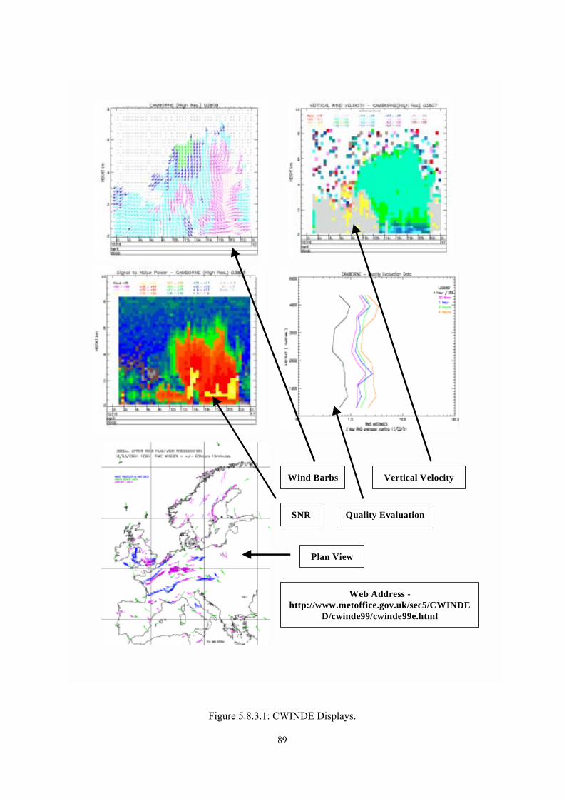
89

Wind Barbs Vertical Velocity

SNR Quality Evaluation

Plan View

Web Address -http://www.metoffice.gov.uk/sec5/CWINDE

D/cwinde99/cwinde99e.html

Figure 5.8.3.1: CWINDE Displays.

90

9. Economic aspects of wind profiler radar In this chapter we try to give an estimate of the total costs of a network of a small number of wind profiler systems. Most of the used figures come from real values with already installed wind profilers, and some figures for long term maintenance and spare parts from estimations. The costs are listed for the three categories of wind profilers, knowing that performance and costs are very different from one category to another. RASS is excluded from costs listed.

Costs that are given represent: • The purchase price of an individual system • The costs for the necessary infrastructure for its installation • The costs of measuring and control equipment for the maintenance personnel to run the

network and initial spare parts • The annual running costs of the system • The annual costs (personnel and spare parts) for the maintenance of the system

Costs for research and development and specific software have been excluded from the figures. Specific software requirements of the individual user can be modifications to the system software for example in the data processing, graphical display etc. or adaptations for the data communication.

It is very complicated to give representative costs for infrastructure. The costs are much higher for a 50 MHz system with the large antenna than for a 1 GHz system. In addition the costs for infrastructure can be small if the system is installed on an existing site, e.g. at an existing upper-air station of a National Meteorological Service or a test field of a research institute or university. But if you have to create a new station or the installation is at an airport, installation costs rise significantly. The figures in the table do not include purchase of land.

The necessary initial service equipment depends on the maintenance and spare parts policy of the network owner. To sustain long term operations without significant data loss a concept has to be developed in co-operation with the manufacturer to guaranty spare parts availability and the necessary maintenance. Either the network operator (usually a National Meteorological Service) organises the maintenance with his own staff, then he needs a larger sum for initial service equipment, or he has a contract with the manufacturer, in which case he needs more money for the yearly maintenance.

We try to summarise the costs for a small network of four systems and the duration of amortisation has been fixed to 20 years for the VHF systems at 50 MHz and UHF at 400-500 MHz, and to 15 years for the 1 GHz UHF systems. After these time periods it is at least necessary to make a major hardware and software upgrade.

In the following tables also the costs for a single profile produced by a wind profiler are given, by taking into account one profile per hour and one profile per fifteen minutes. Compared to aircraft measurements in Europe the costs per profile are of similar magnitude or slightly higher depending on the contractual arrangements and vertical resolutions of the measurements.

The data for theses cost estimates could be collected with the help of the UK Met Office, Météo France, Deutscher Wetterdienst (DWD), KNMI, Austrocontrol, MeteoSwiss and the manufacturers Degreane and Radian.

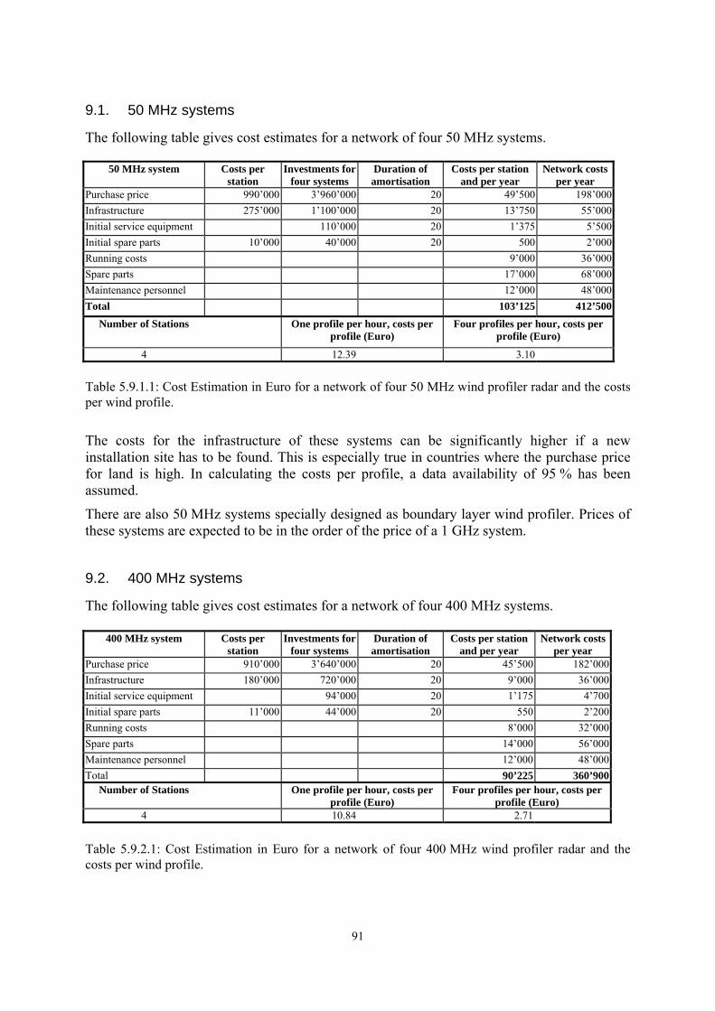
91

9.1. 50 MHz systems

The following table gives cost estimates for a network of four 50 MHz systems.

50 MHz system Costs per station

Investments for four systems

Duration of amortisation

Costs per station and per year

Network costs per year

Purchase price 990�000 3�960�000 20 49�500 198�000Infrastructure 275�000 1�100�000 20 13�750 55�000Initial service equipment 110�000 20 1�375 5�500Initial spare parts 10�000 40�000 20 500 2�000Running costs 9�000 36�000Spare parts 17�000 68�000Maintenance personnel 12�000 48�000Total 103’125 412’500

Number of Stations One profile per hour, costs per profile (Euro)

Four profiles per hour, costs per profile (Euro)

4 12.39 3.10 Table 5.9.1.1: Cost Estimation in Euro for a network of four 50 MHz wind profiler radar and the costs per wind profile.

The costs for the infrastructure of these systems can be significantly higher if a new installation site has to be found. This is especially true in countries where the purchase price for land is high. In calculating the costs per profile, a data availability of 95 % has been assumed.

There are also 50 MHz systems specially designed as boundary layer wind profiler. Prices of these systems are expected to be in the order of the price of a 1 GHz system.

9.2. 400 MHz systems







Purchase price 910�000 3�640�000 20 45�500 182�000Infrastructure 180�000 720�000 20 9�000 36�000Initial service equipment 94�000 20 1�175 4�700Initial spare parts 11�000 44�000 20 550 2�200Running costs 8�000 32�000Spare parts 14�000 56�000Maintenance personnel 12�000 48�000Total 90’225 360’900



4 10.84 2.71 Table 5.9.2.1: Cost Estimation in Euro for a network of four 400 MHz wind profiler radar and the costs per wind profile.

92

The biggest parts of the costs for yearly spare parts are for relays and phase shifters. These components have a life time of about 5 years.

In calculating the costs per profile, a data availability of 95 % has been assumed.

9.3. 1 GHz systems







Purchase price 300�000 1�200�000 15 20�000 80�000Infrastructure 25�000 100�000 15 1�667 6�667Initial service equipment 15�000 15 250 1�000Initial spare parts 5�000 20�000 15 333 1�333Running costs 4�000 16�000Spare parts 14�000 56�000Maintenance personnel 12�000 48�000Total 52’250 209’000



4 6.28 1.57

Table 5.9.3.1: Cost Estimation in Euro for a network of four 1000 MHz wind profiler radar and the costs per wind profile.

Some of the 1 GHz systems are installed at airports for wind shear detection. The installation of these systems may be much more expensive. To facilitate maintenance the profilers operated by Austrocontrol for example are installed in a shelter which costs in addition approximately 80�000 Euro. The data transmission and display has to integrated into the airport environment and requirements on data availability are higher than for other applications.

The biggest parts of the costs for yearly spare parts are for relays and phase shifters which however are not used in some systems. These components have a life time of about 5 years. In calculating the costs per profile, a data availability of 95 % has been assumed.

1

Authors: J. Dibbern, Deutscher Wetterdienst, Germany D. Engelbart, Deutscher Wetterdienst, Germany U. Goersdorf, Deutscher Wetterdienst, Germany N. Latham, Meteorological Office, United Kingdom V. Lehmann, Deutscher Wetterdienst, Germany J. Nash, Meteorological Office, United Kingdom T. Oakley, Meteorological Office, United Kingdom H. Richner, Atmospheric Science, Switzerland H. Steinhagen, Deutscher Wetterdienst, Germany

WORLD ME T E O ROL O GICAL O RGANIZAT I O N … · world me t e o rol o gical o rganizat i o n...

Documents

Transcript of WORLD ME T E O ROL O GICAL O RGANIZAT I O N … · world me t e o rol o gical o rganizat i o n...