Contents lists available at ScienceDirect

Solar Energy

journal homepage: www.elsevier.com/locate/solener

World estimates of PV optimal tilt angles and ratios of sunlight incidentupon tilted and tracked PV panels relative to horizontal panels

Mark Z. Jacobson⁎, Vijaysinh JadhavDepartment of Civil and Environmental Engineering, Stanford University, Stanford, CA 94305-4020, USA

A R T I C L E I N F O

Keywords:Solar photovoltaicsTrackingOptimal tiltSolar radiation

A B S T R A C T

This study provides estimates of photovoltaic (PV) panel optimal tilt angles for all countries worldwide. It thenestimates the incident solar radiation normal to either tracked or optimally tilted panels relative to horizontalpanels globally. Optimal tilts are derived from the National Renewable Energy Laboratory’s PVWatts program. Asimple 3rd-order polynomial fit of optimal tilt versus latitude is derived. The fit matches data better above 40° Nlatitude than do previous linear fits. Optimal tilts are then used in the global 3-D GATOR-GCMOM model toestimate annual ratios of incident radiation normal to optimally tilted, 1-axis vertically tracked (swivelingvertically around a horizontal axis), 1-axis horizontally tracked (at optimal tilt and swiveling horizontallyaround a vertical axis), and 2-axis tracked panels relative to horizontal panels in 2050. Globally- and annually-averaged, these ratios are ∼1.19, ∼1.22, ∼1.35, and ∼1.39, respectively. 1-axis horizontal tracking differsfrom 2-axis tracking, annually averaged, by only 1–3% at most all latitudes. 1-axis horizontal tracking providesmuch more output than 1-axis vertical tracking below 65° N and S, whereas output is similar elsewhere. Trackingprovides little benefit over optimal tilting above 75° N and 60° S. Tilting and tracking benefits generally increasewith increasing latitude. In fact, annually averaged, more sunlight reach tilted or tracked panels from 80 to 90° Sthan any other latitude. Tilting and tracking benefit cities of the same latitude with lesser aerosol and cloudcover. In sum, for optimal utility PV output, 1-axis horizontal tracking is recommended, except for the highestlatitudes, where optimal tilting is sufficient. However, decisions about panel configuration also require knowingtracking equipment and land costs, which are not evaluated here. Installers should also calculate optimal tiltangles for their location for more accuracy. Models that ignore optimal tilting for rooftop PV and utility PVtracking may underestimate significantly country or world PV potential.

1. Introduction

Global solar photovoltaic (PV) installations on rooftops and inpower plants are growing rapidly and will grow further as the worldtransitions from fossil fuels to clean, renewable energy (Jacobson et al.,2017). A critical parameter for installing fixed-tilt panels is the tiltangle, since PV panel output increases with increasing exposure to di-rect sunlight. Energy modelers also need to know the optimal tilt angleof a panel for calculating regional or global PV output in a given lo-cation or worldwide.

Another issue for installers and modelers is whether 1-axis verticaltracked PV panels (panels that face south or north and swivel verticallyaround a horizontal axis) receive more incident radiation than 1-axishorizontal tracked panels (panels at optimal tilt angle that swivel hor-izontally around a vertical axis), and the extent to which incident ra-diation to 1-axis- and 2-axis-tracked panels (which combine 1-axisvertical and horizontal tracking capabilities to follow the sun perfectly

during the day) exceeds that of optimally tilted panels. Finally, becauseglobal and regional weather and climate models almost all calculateradiative transfer assuming that radiation impinges on horizontal sur-faces, energy modelers also need estimates of the ratio of incident solarradiation to panels that track the sun or are optimally-tilted to that ofpanels that are placed horizontally on a flat surface.

This study first provides estimates of optimal tilt angles derivedfrom the NREL PVWatts program (NREL, 2017) at 1–4 sites in eachcountry of the world. These optimal tilt angles are representative ofassumed historic meteorological conditions near a given site, so areonly approximate. Although installers would need to make more precisecalculations at each site, the results provided here are still useful roughestimates. The study then provides convenient albeit rough polynomialfits to the PVWatts data of the optimal tilt angle as a function of latitudefor both the Northern and Southern Hemispheres. The optimal tilt databy country and by latitude are then input into a global climate model,GATOR-GCMOM for year 2050 meteorological and air quality

https://doi.org/10.1016/j.solener.2018.04.030Received 18 December 2017; Received in revised form 4 April 2018; Accepted 13 April 2018

⁎ Corresponding author.E-mail address: jacobson@stanford.edu (M.Z. Jacobson).

Solar Energy 169 (2018) 55–66

0038-092X/ © 2018 Elsevier Ltd. All rights reserved.

T

conditions, to provide ratios of incident solar radiation normal to anoptimally tilted, 1-axis vertically-tracked, 1-axis horizontally-tracked,and 2-axis tracked PV panel relative to a horizontal panel.

The reasons for using GATOR-GCMOM rather than PVWatts for theglobal calculations are (1) GATOR-GCMOM covers the entire world,whereas PVWatts covers locations only near specific meteorologicalstations, (2) GATOR-GCMOM is used here to examine a future 2050scenario, where aerosol, cloud, temperature, and wind speed propertiesdiffer from today, whereas PVWatts treats only past conditions, and (3)we want to use GATOR-GCMOM to calculate incident solar radiation forthe two components of 1-axis horizontal tracking that, when combined,exactly comprise the components of 2-axis tracking, and this cannot bedone with current PVWatts output. Specifically, one way for a panel tofollow the sun exactly throughout the day (2-axis tracking), is for thepanel to swivel horizontally around a vertical axis and, independently,swivel vertically around a horizontal axis. In this study, we calculateincident radiation for both cases – namely vertical tracking (swivelingvertically around a horizontal axis with the panel facing south or north)and horizontal tracking (swiveling horizontally around a vertical axiswith the panel at optimal south-north tilt), and separately calculateincident radiation for 2-axis tracking. Whereas PVWatts calculates in-cident radiation for 2-axis tracking, it does not consider either of theabove 1-axis options; instead, it invokes a third option, which is toswivel east-to-west around an axis parallel to a specified tilt, not ne-cessarily the optimal tilt, of the panel. That option is not examined here,but the 1-axis horizontal tracking option treated here results in incidentradiation within 1–3% of the 2-axis tilting option at most latitudes, thusmay be close to optimal, if not optimal, for 1-axis tracking.

Many studies have provided equations that allow for the theoreticalcalculation of the optimal tilt angle over time of a solar collector basedon Earth-sun geometry (e.g., Kern and Harris, 1975; Koronakis, 1986;Lewis, 1987; Gunerhan and Hepbash, 2009; Chang, 2009; Talebizadehet al., 2011; Yadav and Chandel, 2013). Some of these studies havederived simple linear expressions of optimal tilt angle versus latitude(Chang, 2009; Talebizadeh et al., 2011). However, optimal tilt dependsnot only on latitude but also on weather conditions, including cloudcover (Kern and Harris, 1975) and the altitude above sea level (Yadavand Chandel, 2013). Because of the difficulty in determining optimaltilt angle as a function of cloud cover and weather conditions, calcu-lators such as PVWatts (NREL, 2017), are often used to estimate optimaltilt angles at specific locations (Yadav and Chandel, 2013). Here, wefirst use PVWatts to estimate 1–4 optimal tilt angles for each country ofthe world.

Breyer and Schmid (2010a) combined satellite data with geometricand radiative equations to map global estimates of optimal tilt anglesfor solar PV. Similarly, Breyer and Schmid (2010a, 2010b), Breyer(2012), Bogdanov and Breyer (2016), Kilickaplan et al. (2017), Breyeret al. (2017a, 2017b), Sadiqa et al. (2018) have applied tilting, single-axis, and/or 2-axis tracking equations to regionally- or globally-griddedsolar radiation satellite datasets for energy analysis. However, it ap-pears that no 3-D global or regional climate, weather, or air pollutionmodel has included tilting, 1-axis horizontal tracking, 1-axis verticaltracking, or 2-axis tracking interactively within it. Pelland et al. (2011)used horizontal-plate solar radiation output from a downscaled climatemodel to estimate PV output from fixed-tilt panels. However, the cal-culation was done offline (after the 3-D model simulation was per-formed) rather than online (interactive within the 3-D model), thus itcould not examine the effects of, for example, instantaneous tempera-ture and wind speed, on panel performance. This study offers the op-portunity to estimate global PV output anywhere in the world withtilted or tracked panels relative to horizontal panels using consistentmeteorology and accounting for temperature and wind speed on panelperformance.

The ideal tracking or tilting option depends not only on the incidentsolar radiation relative to a horizontal surface but also on the land orroof area needed to avoid shading, and the cost of tracking versus

tilting. For example, 2-axis tracking in a utility PV plant requires moreland area to avoid shading panels behind the front row than do 1-axistracking or optimal tilting, and 2-axis equipment is more expensivethan is 1-axis equipment or optimal tilting. Shading depends not onlyon panel tilting, but also on the height that panels are placed relative toeach other. For example, panels that track the sun placed on a south-facing hillside will likely see less shading than will panels on uniformlyelevated ground. Shading further depends on the number of panelsplaced on each single platform that tracks the sun. In sum, the decisionabout what type of tracking or tilting option is best ultimately dependsnot only on the incident radiation received normal to each panel, butalso on the land or roof area required to avoid shading and on the cost.In this study, we examine only the ratios of incident radiation withdifferent tilting and tracking options relative to horizontal panels. Wedo not consider areas required or costs. However, these topics are dis-cussed at length in Breyer (2012).

2. Methodology for determining optimal tilt angles

We first use PVWatts (NREL, 2017), which combines solar resourcedata from a specific location with 30 years of historic temperature andwind speed data from a nearby meteorological station, characteristics ofa solar panel, and orientation of the panel relative to the sun. PVWattsuses ‘typical year’ meteorology from each station, which is relevant,since the data have considerable inter-annual variability. For example,in the U.S., solar output during the lowest 10th percentile solar outputmeteorological year is on average, 4.8% less than that during the 50thpercentile year (Ryberg et al., 2015). PVWatts uses solar data from theNational Solar Radiation Database 1961–1990 for the U.S., the Cana-dian Weather for Energy Calculations database for Canada, and bothASHRAE International Weather for Energy Calculations Version 1.1data and Solar and Wind Energy Resource Assessment Program data forall other countries. “Typical year” solar radiation values from thesedatabases are updated by PVWatts to account for the reduction insunlight due to clouds and air pollution at each site. Panel altitude,latitude, longitude, and angle relative to the sun are used to estimateexposure of the panel to sunlight. Air temperature and wind speed dataare used to estimate panel temperature.

Here, PVWatts is used to estimate annually averaged solar output inall countries of the world assuming tilted panels. The optimal tilt anglein each location is found by calculating panel output with different tiltangles until the tilt angle giving the maximum output is found. That tiltangle is the optimal tilt angle. In most countries, an optimal tilt angle isestimated for only one location. For several large countries, estimatesare obtained for 2–4 locations (Table 1). The optimal tilt angles cal-culated here are not necessarily the most cost-effective fixed tilt anglesbecause they do not account for the additional land needed to minimizeshading between panels (Section 3.2 of Breyer (2012)).

The main assumptions for the calculations with PVWatts include thefollowing: 10 kW of premium panels with a temperature coefficient of−0.0035/K and 10% efficiency losses. Such losses include soiling (2%),wiring (2%), connections (0.5%), mismatch (2%), light-induced de-gradation (1.5%), nameplate rating (1%), shading (0.5%), and avail-ability (0.5%). All panels are assumed to face due south in the NorthernHemisphere (180° azimuth angle) or due north in the Southern hemi-sphere (0° azimuth angle), with the exception of Nairobi, Kenya, whichis slightly in the Southern Hemisphere (−1.32 S), but has an optimaltilt angle calculated to face 4° southward.

3. Optimal tilt angle results

Table 1 provides all optimal tilt angle results from PVWatts. Fig. 1shows the resulting optical tilt angles versus latitude for each locationin each country of the world in Table 1. The results are approximate foreach location, so installers would need to make more exact calculationsat their location of interest. 3rd-order polynomials are fit through the

M.Z. Jacobson, V. Jadhav Solar Energy 169 (2018) 55–66

56

Table 1Optimal tilt angles for fixed tilt solar PV panels for all countries of the world.

Country Representative City Nearest Meteorological Station Station Lat. (deg.) StationLon. (deg.) Opt tilt

Iceland Reykjavík Reykjavík 64.13 −21.9 43Afghanistan Kandahar Karachi, Pakistan 24.9 67.13 25Albania Sarande S Maria Di Leuca 39.65 18.35 30Algeria Algiers Algiers 36.72 3.25 31Andorra Andorra La Vella Gerona, Spain 41.9 2.77 37Angola Luanda Harare, Zimbabwe −17.92 31.13 −22Antigua and Barbuda St. Johns Fort-De-France 14.6 −61 14Argentina Buenos Aires Buenos Aires −34.82 −58.53 −30Armenia Yerevan Tabriz, Iran 38.05 46.17 30Australia Darwin Darwin −12.42 130.88 −18Australia Perth Perth −31.93 115.95 −27Australia Sydney Sydney −33.95 151.18 −31Austria Graz Graz 47 15.43 33Azerbaijan Lankaran Tabriz, Iran 38.05 46.17 30Bahamas Nassau Saua La Grande 22.82 −80.08 21Bahrain Riffa Riyadh 24.7 46.8 26Bangladesh Chittagong Chittagong 22.27 91.82 25Barbados Bridgetown Fort-De-France 14.6 −61 14Belarus Minsk Minsk 53.87 27.53 32Belgium Saint Hubert Saint Hubert 50.03 5.4 35Belize Belize City Belize 17.53 −88.3 16Benin Port Novo Accra, Ghana 5.6 −0.17 6a

Bhutan Thimphu Pagri, China 27.73 89.08 32Bolivia La Paz La Paz −16.52 −68.18 −22Bosnia Herzegovina Banja Luka Banja Luka 44.78 17.22 33Botswana Gaborone Johannesburg −26.13 28.23 −29Brazil Manaus Manaus −3.13 −60.02 −7a

Brazil Rio De Janeiro Rio De Janeiro −22.9 −43.17 −22Brunei Darussalam Bandar Seri Begaw Bandar Seri Begawan 4.93 114.93 5a

Bulgaria Plovdiv Plovdiv 42.13 24.75 30Burkina Faso Banfora Accra, Ghana 5.6 −0.17 6a

Burundi Bujumbura Kisii, Kenya −0.67 34.78 −3a

Cabo Verde Praia Dakar, Senegal 14.73 −17.5 14Cambodia Phnom Penh Bangkok, Thailand 13.92 100.6 15Cameroon Douala Accra, Ghana 5.6 −0.17 6a

Canada Calgary Calgary 51.12 −114.02 45Canada Vancouver Vancouver 49.18 −123.17 34Canada Montreal Montreal 45.5 −73.62 37Central Afr. Republic Carnot Accra, Ghana 5.6 −0.17 6a

Chad N'Djamena Accra, Ghana 5.6 −0.17 6a

Chile Antofagasta Antofagasta −23.43 −70.43 −22China Beijing Beijing 39.93 116.28 37China Shanghai Shanghai 31.17 121.43 23China Lhasa Lhasa 29.67 91.13 31China Kunming Kunming 25.02 102.68 25Colombia Bogota Bogota 4.7 −74.13 5a

Comoros Moroni Antananarivo −18.8 47.48 −18Congo Owando Accra, Ghana 5.6 −0.17 6a

Congo Dem Rep of Lubumbashi Harare, Zimbabwe −17.92 31.13 −22Costa-Rica San Jose Rivas, Nicaragua 11.42 85.83 14Croatia Zadar Ancona, Italy 43.62 13.37 30Cuba Sancti Spiritus Sancti Spiritus 21.93 −79.45 21Cyprus Larnaca Larnaca 34.88 33.63 30Czech Republic Ostrava Ostrava 49.72 18.18 33Denmark Copenhagen Copenhagen 55.63 12.67 36Djibouti Djibouti Combolcha/Dessie 11.08 39.72 15Dominica Roseau Fort-De-France 14.6 −61 14Dominican Republic Santo Domingo Aquadilla Borinquen 18.5 −67.13 20Dutch-Antilles Willemstad Caracas, Venezuela 10.6 −66.98 10Ecuador Quito Quito −0.15 −78.48 −3a

Egypt Aswan Aswan 23.97 32.78 24El Salvador Ilopango Ilopango 13.7 −89.12 18Equatorial Guinea Bata Accra, Ghana 5.6 −0.17 6a

Eritrea Keren Gondar, Ethiopia 12.53 37.43 18Estonia Tartu Helsinki, Finland 60.32 24.97 39Ethiopia Gondar Gondar 12.53 37.43 18Fiji Nadi Nadi −17.75 177.45 −18Finland Helsinki Helsinki 60.32 24.97 39France Lyon Lyon 45.73 5.08 30France Bordeaux Bordeaux 44.83 −0.7 33Gabon Libreville Accra, Ghana 5.6 −0.17 6a

Gambia Banjul Dakar, Senegal 14.73 −17.5 14Georgia Tbilisi Tabriz, Iran 38.05 46.17 30Germany Cologne Cologne 50.87 7.17 32

(continued on next page)

M.Z. Jacobson, V. Jadhav Solar Energy 169 (2018) 55–66

57

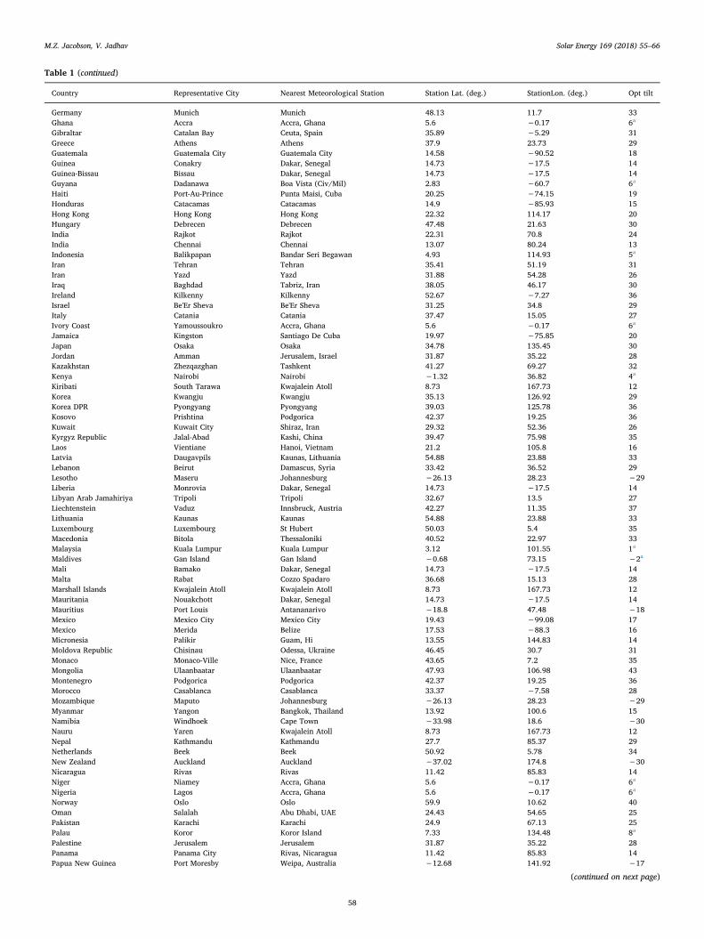
Table 1 (continued)

Country Representative City Nearest Meteorological Station Station Lat. (deg.) StationLon. (deg.) Opt tilt

Germany Munich Munich 48.13 11.7 33Ghana Accra Accra, Ghana 5.6 −0.17 6a

Gibraltar Catalan Bay Ceuta, Spain 35.89 −5.29 31Greece Athens Athens 37.9 23.73 29Guatemala Guatemala City Guatemala City 14.58 −90.52 18Guinea Conakry Dakar, Senegal 14.73 −17.5 14Guinea-Bissau Bissau Dakar, Senegal 14.73 −17.5 14Guyana Dadanawa Boa Vista (Civ/Mil) 2.83 −60.7 6a

Haiti Port-Au-Prince Punta Maisi, Cuba 20.25 −74.15 19Honduras Catacamas Catacamas 14.9 −85.93 15Hong Kong Hong Kong Hong Kong 22.32 114.17 20Hungary Debrecen Debrecen 47.48 21.63 30India Rajkot Rajkot 22.31 70.8 24India Chennai Chennai 13.07 80.24 13Indonesia Balikpapan Bandar Seri Begawan 4.93 114.93 5a

Iran Tehran Tehran 35.41 51.19 31Iran Yazd Yazd 31.88 54.28 26Iraq Baghdad Tabriz, Iran 38.05 46.17 30Ireland Kilkenny Kilkenny 52.67 −7.27 36Israel Be'Er Sheva Be'Er Sheva 31.25 34.8 29Italy Catania Catania 37.47 15.05 27Ivory Coast Yamoussoukro Accra, Ghana 5.6 −0.17 6a

Jamaica Kingston Santiago De Cuba 19.97 −75.85 20Japan Osaka Osaka 34.78 135.45 30Jordan Amman Jerusalem, Israel 31.87 35.22 28Kazakhstan Zhezqazghan Tashkent 41.27 69.27 32Kenya Nairobi Nairobi −1.32 36.82 4a

Kiribati South Tarawa Kwajalein Atoll 8.73 167.73 12Korea Kwangju Kwangju 35.13 126.92 29Korea DPR Pyongyang Pyongyang 39.03 125.78 36Kosovo Prishtina Podgorica 42.37 19.25 36Kuwait Kuwait City Shiraz, Iran 29.32 52.36 26Kyrgyz Republic Jalal-Abad Kashi, China 39.47 75.98 35Laos Vientiane Hanoi, Vietnam 21.2 105.8 16Latvia Daugavpils Kaunas, Lithuania 54.88 23.88 33Lebanon Beirut Damascus, Syria 33.42 36.52 29Lesotho Maseru Johannesburg −26.13 28.23 −29Liberia Monrovia Dakar, Senegal 14.73 −17.5 14Libyan Arab Jamahiriya Tripoli Tripoli 32.67 13.5 27Liechtenstein Vaduz Innsbruck, Austria 42.27 11.35 37Lithuania Kaunas Kaunas 54.88 23.88 33Luxembourg Luxembourg St Hubert 50.03 5.4 35Macedonia Bitola Thessaloniki 40.52 22.97 33Malaysia Kuala Lumpur Kuala Lumpur 3.12 101.55 1a

Maldives Gan Island Gan Island −0.68 73.15 −2a

Mali Bamako Dakar, Senegal 14.73 −17.5 14Malta Rabat Cozzo Spadaro 36.68 15.13 28Marshall Islands Kwajalein Atoll Kwajalein Atoll 8.73 167.73 12Mauritania Nouakchott Dakar, Senegal 14.73 −17.5 14Mauritius Port Louis Antananarivo −18.8 47.48 −18Mexico Mexico City Mexico City 19.43 −99.08 17Mexico Merida Belize 17.53 −88.3 16Micronesia Palikir Guam, Hi 13.55 144.83 14Moldova Republic Chisinau Odessa, Ukraine 46.45 30.7 31Monaco Monaco-Ville Nice, France 43.65 7.2 35Mongolia Ulaanbaatar Ulaanbaatar 47.93 106.98 43Montenegro Podgorica Podgorica 42.37 19.25 36Morocco Casablanca Casablanca 33.37 −7.58 28Mozambique Maputo Johannesburg −26.13 28.23 −29Myanmar Yangon Bangkok, Thailand 13.92 100.6 15Namibia Windhoek Cape Town −33.98 18.6 −30Nauru Yaren Kwajalein Atoll 8.73 167.73 12Nepal Kathmandu Kathmandu 27.7 85.37 29Netherlands Beek Beek 50.92 5.78 34New Zealand Auckland Auckland −37.02 174.8 −30Nicaragua Rivas Rivas 11.42 85.83 14Niger Niamey Accra, Ghana 5.6 −0.17 6a

Nigeria Lagos Accra, Ghana 5.6 −0.17 6a

Norway Oslo Oslo 59.9 10.62 40Oman Salalah Abu Dhabi, UAE 24.43 54.65 25Pakistan Karachi Karachi 24.9 67.13 25Palau Koror Koror Island 7.33 134.48 8a

Palestine Jerusalem Jerusalem 31.87 35.22 28Panama Panama City Rivas, Nicaragua 11.42 85.83 14Papua New Guinea Port Moresby Weipa, Australia −12.68 141.92 −17

(continued on next page)

M.Z. Jacobson, V. Jadhav Solar Energy 169 (2018) 55–66

58

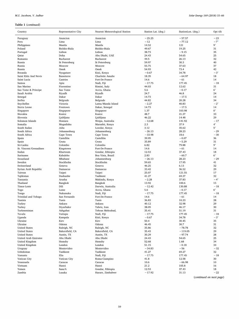
Table 1 (continued)

Country Representative City Nearest Meteorological Station Station Lat. (deg.) StationLon. (deg.) Opt tilt

Paraguay Asuncion Asuncion −25.25 −57.57 −23Peru Lima Lima −12 −77.12 −7a

Philippines Manila Manila 14.52 121 9a

Poland Bielsko-Biala Bielsko-Biala 49.67 19.25 31Portugal Lisbon Lisbon 38.73 −9.15 35Qatar Doha Abu Dhabi, UAE 24.43 54.65 25Romania Bucharest Bucharest 44.5 26.13 32Russia St Petersburg St Petersburg 59.97 30.3 40Russia Moscow Moscow 55.75 37.63 37Russia Omsk Omsk 54.93 73.4 42Rwanda Nyagatare Kisii, Kenya −0.67 34.78 −3a

Saint Kitts And Nevis Basseterre Charlotte Amalie 18.35 −64.97 18Saint Lucia Castries Fort-De-France 14.6 −61 14Samoa Apia Nadi, Fiji −17.75 177.45 −18San Marino Fiorentino Rimini, Italy 44.03 12.62 31Sao Tome & Principe Sao Tome Accra, Ghana 5.6 −0.17 6a

Saudi Arabia Riyadh Riyadh 24.7 46.8 24Senegal Dakar Dakar 14.73 −17.5 14Serbia Belgrade Belgrade 44.82 20.28 34Seychelles Victoria Lamu/Manda Island −2.27 40.83 −2a

Sierra Leone Freetown Dakar, Senegal 14.73 −17.5 14Singapore Singapore Singapore 1.37 103.98 0a

Slovakia Kosice Kosice 48.7 21.27 33Slovenia Ljubljana Ljubljana 46.22 14.48 29Solomon Islands Honiara Weipa, Australia −12.68 141.92 −17Somalia Mogadishu Marsabit, Kenya 2.3 37.9 4a

South Sudan Juba Lowdar, Kenya 3.12 35.62 5a

South Africa Johannesburg Johannesburg −26.13 28.23 −29South Africa Cape Town Cape Town −33.98 18.6 −30Spain Castellón Castellón 39.95 −0.07 36Spain Ceuta Ceuta 35.89 −5.29 31Sri-Lanka Colombo Colombo 6.82 79.88 9a

St. Vincent/Grenadines Kingstown Fort-De-France 14.6 −61 14Sudan Khartoum Gondar, Ethiopia 12.53 37.43 18Suriname Kabalebo Boa Vista, Brazil 2.83 −60.7 6a

Swaziland Mbabane Johannesburg −26.13 28.23 −29Sweden Stockholm Stockholm 59.65 17.95 41Switzerland Geneva Geneva 46.25 6.13 32Syrian Arab Republic Damascus Damascus 33.42 36.52 29Taiwan Taipei Taipei 25.07 121.55 17Tajikistan Dushanbe Tashkent 41.27 69.27 32Tanzania Arusha Makindu, Kenya −2.28 37.83 −4a

Thailand Bangkok Bangkok 13.92 100.6 15Timor-Leste Dili Darwin, Australia −12.42 130.88 −18Togo Lome Accra, Ghana 5.6 −0.17 6a

Tonga Nukunuku Nadi, Fiji −17.75 177.45 −18Trinidad and Tobago San Fernando Fort-De-France 14.6 −61 14Tunisia Tunis Tunis 36.83 10.23 28Turkey Ankara Ankara 40.12 32.98 29Turkey Diyarbakır Tabriz, Iran 38.05 46.17 30Turkmenistan Ashgabat Tehran Mehrabad, 35.41 51.19 31Tuvalu Vaitupu Nadi, Fiji −17.75 177.45 −18Uganda Kampala Kisii, Kenya −0.67 34.78 −3a

Ukraine Kiev Kiev 50.4 30.45 35Ukraine Odessa Odessa 46.45 30.7 31United States Raleigh, NC Raleigh, NC 35.86 −78.78 32United States Bakersfield, CA Bakersfield, CA 35.43 −119.05 29United States Austin, TX Austin, TX 30.29 −97.74 28United Arab Emirates Abu Dhabi Abu Dhabi 24.43 54.65 25United Kingdom Hemsby Hemsby 52.68 1.68 34United Kingdom London London 51.15 −0.18 34Uruguay Montevideo Montevideo −34.83 −56 −32Uzbekistan Tashkent Tashkent 41.27 69.27 32Vanuatu Elia Nadi, Fiji −17.75 177.45 −18Vatican City Vatican City Roma-Ciampino 41.8 12.58 30Venezuela Caracas Caracas 10.6 −66.98 10Vietnam Hanoi Hanoi 21.2 105.8 16Yemen Sana'A Gondar, Ethiopia 12.53 37.43 18Zambia Lusaka Harare, Zimbabwe −17.92 31.13 −22

(continued on next page)

M.Z. Jacobson, V. Jadhav Solar Energy 169 (2018) 55–66

59

data in each hemisphere. Fig. 1 also shows results from two linear es-timates of optimal tilt angle versus latitude from Chang (2009) andTalebizadeh et al. (2011). For most mid-latitude values, the linear es-timates and the polynomial fit track the PVWatts optimal tilt angleswell.

However, for high latitudes in the Northern Hemisphere, the linearfits diverge substantially for most, but not all data. The reason is thatthe linear estimates ignore cloud cover and air pollution, but in reality,heavy cloud cover and haze exist in many high-latitude countries andregions. Greater cloud cover results in lower optimal tilt angles becauseclouds scatter solar radiation isotropically, so the closer a panel is to thehorizontal under cloudy skies, the more diffuse solar radiation it willreceive that is scattered by clouds above them. Further, the directcomponent of solar radiation, which depends significantly on tilt angle,is largely blocked by clouds, so the diffuse component becomes moreimportant when clouds are present. In sum, on average, the 3rd-orderpolynomial fit derived here appears to represent better the optimal tiltangle of solar panels above around 40° N latitude than some previouslinear functions do.

However, the linear functions do estimate optimal tilt better thanthe polynomial fit at a few high-latitude locations that have relativelyclear sky. For example, Calgary (51.12° N), has a higher optimal tiltangle (45°) than does Beek, the Netherlands (34°), which is at a similarlatitude (50.92° N). The reason, as explained above, is that Calgary isexposed to less cloud cover so panels can more efficiently take ad-vantage of overhead sun. In Beek, due to heavier cloud cover, panels are

exposed to less direct light, so must take advantage of isotropic diffuselight scattered by clouds above them and receive more of such lightwith a lower optimal tilt angle. Other data (Breyer and Schmid, 2010a)similarly indicate that optimal tilt angles vary substantially at the samelatitude but different longitude, in many parts of the world.

Calgary, in fact, benefits the most from tilting and tracking amongall locations examined with PVWatts. Solar output there is ∼32.4%higher with optimal tilting than with horizontal panels (no tilting) and91.4% higher with 2-axis tracking than with no tilting. In Beek, optimaltilting yields only 14.6% greater output than with no tilting, and 2-axistracking yields only 34.8% greater output than with no tilting. Trackingand tilting both benefit Calgary the most in January (ratio of 2-axis:notilt of 3.44 and optimal tilt:no tilt of 2.68) and the least in June (1.51and 0.93). Tracking and tilting benefit Beek the most in December(ratio of 2-axis:no tilt of 1.97 and optimal tilt:no tilt of 1.64) and theleast in June (1.14 and 0.98).

The difference between Calgary and Beek is due entirely to thegreater cloudiness (Anderson and West, 2017) and aerosol pollution(The World Bank, 2017) in the Netherlands than in Canada, and aerosolpollution enhances cloud optical thickness. Conversely, reducingaerosol pollution reduces cloudiness and increases surface solar radia-tion. For example, between 1980 and 2005, surface solar radiation inEurope increased about 10W/m2 (Ohmura, 2009). The reason is that,between 1985 and 2007, aerosol optical depth over Europe declined69%, increasing surface solar radiation (Chiacchio et al., 2011). Feweraerosol particles result in clouds being optically thinner due to the first

Table 1 (continued)

Country Representative City Nearest Meteorological Station Station Lat. (deg.) StationLon. (deg.) Opt tilt

Zimbabwe Harare Harare −17.92 31.13 −22

a Indicates the optimal tilt angle is between +/−10°, thus panels will likely be tilted in practice either +10° for positive values or −10° for negative values toallow for rain to naturally wash them.Data are derived from PVWatts (NREL, 2017). The meteorological station used for radiation and meteorological data and its latitude and longitude are also shown.The optimal tilt angles are calculated assuming all panels are roof mount, premium panels with rated power of 10 kW, system losses of 10%, and facing due south inthe Northern Hemisphere (180° azimuth angle, positive optimal tilt angle) or north in the Southern Hemisphere (0° azimuth angle, negative optimal tilt angle). In onecase (Kenya), which is slightly in the Southern Hemisphere, the optimal tilt angle is facingl slightly south, thus negative. Calculations for several countries, parti-cularly island countries, are based on the same meteorological station, since it is the nearest available, thus all output and tilt angles are the same. Such duplicatevalues are removed in all figures and in the derivation of all fitting curves. For some large countries geographically, results are shown for 2–4 locations.

0

10

20

30

40

50

60

70

0

10

20

30

40

50

60

70

0 8 16 24 32 40 48 56 64

C09: 2.14+ ϕ0.764

T11: 7.203+ ϕ0.6804

This study: 1.3793+ ϕ(1.2011+ ϕ(-0.014404+ϕ0.000080509)) (R=0.96)

Opt

imal

Tilt

Ang

le (d

egre

es)

Latitude (degrees)

Northern Hemisphere-50

-40

-30

-20

-10

0

10

-50

-40

-30

-20

-10

0

10

-50 -40 -30 -20 -10 0

C09: -2.14+ ϕ0.764T11: -7.203+ ϕ0.6804This study:-0.41657+ ϕ(1.4216+ ϕ(0.024051+ϕ0.00021828)) (R=0.97)

Opt

imal

Tilt

Ang

le (d

egre

es)

Latitude (degrees)

Southern Hemisphere

Fig. 1. Estimated optimal tilt angles and 3rd-order polynomial fits through them of fixed-tilt solar collectors for all countries in the Northern Hemisphere andSouthern Hemisphere, as derived from PVWatts. Data for each country are from Table 1. Countries with identical tilt angles in Table 1, due to the fact that they relyon the same meteorological station as other countries, are excluded from the figure and curve fits. Also shown are linear equations from two previous studies, Chang[7, C09] and Talebizadeh [8, T11], where φ is latitude (in degrees). To allow for rain to naturally clean panels, optimal tilt angles between −10 and +10° latitudeare usually limited to either −10° (for negative values) or +10° (for positive values).

M.Z. Jacobson, V. Jadhav Solar Energy 169 (2018) 55–66

60

indirect effect of aerosol particles on clouds. Because aerosol pollutionis likely to drop further between now and 2050, solar output is likely toincrease further by 2050. Since PVWatts relies on 30 years of pastmeteorological data and recent solar radiation data, it may thus un-derestimate 2050 solar resource in any currently polluted region of theworld.

In practice, when the optimal tilt angle is between −10 and +10°,which occurs primarily in the tropics, installers generally tilt the paneleither −10 or +10° to allow for rainfall to naturally cleanse the panels.The locations that this affects are denoted in Table 1.

4. Calculating incident solar radiation with GATOR-GCMOM

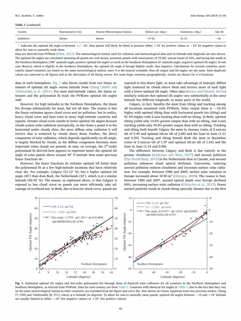
The 3rd-order optimal tilt polynomials as a function of latitude(Fig. 1), derived from PVWatts data, were input worldwide into everygrid cell in the global weather-climate-air-pollution model GATOR-GCMOM (Gas, Aerosol, Transport, Radiation, General Circulation, Me-soscale, and Ocean Model) (Jacobson, 2001a, 2001b, 2005, 2012;Jacobson et al., 2007, 2014; Jacobson and Archer, 2012). All individualoptimal tilts from Table 1 within 700 km to the west or east and within250 km to the south or north of a grid cell horizontal center were theninterpolated to each cell center using a 1/R2 interpolation (whereR= distance from the cell center to the data point) and using thebackground value as one data point 700 km×250 km away. This in-terpolation resulted in values from Table 1 dominating near the loca-tions in Table 1 but also in background values dominating over oceanwater and over land away from the locations in Table 1. Fig. 2 showsthe resulting worldwide field, which was input into GATOR-GCMOM.Fig. 2 does not reflect GATOR-GCMOM meteorology, only values fromPVWatts. Fig. 2 does not show more variation with longitude becausethe number of locations with specific optimal tilt values in Table 1 isrelatively small, particularly for big countries, and no locations are overthe ocean. PVWatts itself was not used in GATOR-GCMOM.

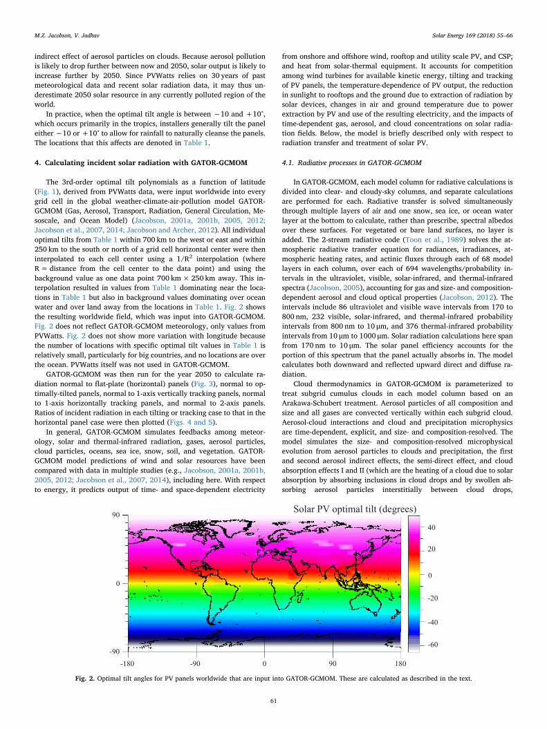
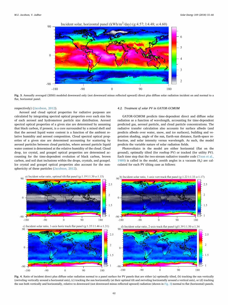
GATOR-GCMOM was then run for the year 2050 to calculate ra-diation normal to flat-plate (horizontal) panels (Fig. 3), normal to op-timally-tilted panels, normal to 1-axis vertically tracking panels, normalto 1-axis horizontally tracking panels, and normal to 2-axis panels.Ratios of incident radiation in each tilting or tracking case to that in thehorizontal panel case were then plotted (Figs. 4 and 5).

In general, GATOR-GCMOM simulates feedbacks among meteor-ology, solar and thermal-infrared radiation, gases, aerosol particles,cloud particles, oceans, sea ice, snow, soil, and vegetation. GATOR-GCMOM model predictions of wind and solar resources have beencompared with data in multiple studies (e.g., Jacobson, 2001a, 2001b,2005, 2012; Jacobson et al., 2007, 2014), including here. With respectto energy, it predicts output of time- and space-dependent electricity

from onshore and offshore wind, rooftop and utility scale PV, and CSP;and heat from solar-thermal equipment. It accounts for competitionamong wind turbines for available kinetic energy, tilting and trackingof PV panels, the temperature-dependence of PV output, the reductionin sunlight to rooftops and the ground due to extraction of radiation bysolar devices, changes in air and ground temperature due to powerextraction by PV and use of the resulting electricity, and the impacts oftime-dependent gas, aerosol, and cloud concentrations on solar radia-tion fields. Below, the model is briefly described only with respect toradiation transfer and treatment of solar PV.

4.1. Radiative processes in GATOR-GCMOM

In GATOR-GCMOM, each model column for radiative calculations isdivided into clear- and cloudy-sky columns, and separate calculationsare performed for each. Radiative transfer is solved simultaneouslythrough multiple layers of air and one snow, sea ice, or ocean waterlayer at the bottom to calculate, rather than prescribe, spectral albedosover these surfaces. For vegetated or bare land surfaces, no layer isadded. The 2-stream radiative code (Toon et al., 1989) solves the at-mospheric radiative transfer equation for radiances, irradiances, at-mospheric heating rates, and actinic fluxes through each of 68 modellayers in each column, over each of 694 wavelengths/probability in-tervals in the ultraviolet, visible, solar-infrared, and thermal-infraredspectra (Jacobson, 2005), accounting for gas and size- and composition-dependent aerosol and cloud optical properties (Jacobson, 2012). Theintervals include 86 ultraviolet and visible wave intervals from 170 to800 nm, 232 visible, solar-infrared, and thermal-infrared probabilityintervals from 800 nm to 10 μm, and 376 thermal-infrared probabilityintervals from 10 μm to 1000 μm. Solar radiation calculations here spanfrom 170 nm to 10 μm. The solar panel efficiency accounts for theportion of this spectrum that the panel actually absorbs in. The modelcalculates both downward and reflected upward direct and diffuse ra-diation.

Cloud thermodynamics in GATOR-GCMOM is parameterized totreat subgrid cumulus clouds in each model column based on anArakawa-Schubert treatment. Aerosol particles of all composition andsize and all gases are convected vertically within each subgrid cloud.Aerosol-cloud interactions and cloud and precipitation microphysicsare time-dependent, explicit, and size- and composition-resolved. Themodel simulates the size- and composition-resolved microphysicalevolution from aerosol particles to clouds and precipitation, the firstand second aerosol indirect effects, the semi-direct effect, and cloudabsorption effects I and II (which are the heating of a cloud due to solarabsorption by absorbing inclusions in cloud drops and by swollen ab-sorbing aerosol particles interstitially between cloud drops,

-60

-40

-20

0

20

40

-180 -90 0 90 180-90

0

90Solar PV optimal tilt (degrees)

Fig. 2. Optimal tilt angles for PV panels worldwide that are input into GATOR-GCMOM. These are calculated as described in the text.

M.Z. Jacobson, V. Jadhav Solar Energy 169 (2018) 55–66

61

respectively) (Jacobson, 2012).Aerosol and cloud optical properties for radiative purposes are

calculated by integrating spectral optical properties over each size binof each aerosol and hydrometeor particle size distribution. Aerosolspectral optical properties of a given size are determined by assumingthat black carbon, if present, is a core surrounded by a mixed shell andthat the aerosol liquid water content is a function of the ambient re-lative humidity and aerosol composition. Cloud spectral optical prop-erties of a given size are determined accounting for scattering byaerosol particles between cloud particles, where aerosol particle liquidwater content is determined at the relative humidity of the cloud. Clouddrop, ice crystal, and graupel optical properties are determined ac-counting for the time-dependent evolution of black carbon, browncarbon, and soil dust inclusions within the drops, crystals, and graupel.Ice crystal and graupel optical properties also account for the non-sphericity of these particles (Jacobson, 2012).

4.2. Treatment of solar PV in GATOR-GCMOM

GATOR-GCMOM predicts time-dependent direct and diffuse solarradiation as a function of wavelength, accounting for time-dependentpredicted gas, aerosol particle, and cloud particle concentrations. Theradiative transfer calculation also accounts for surface albedo (andpredicts albedo over water, snow, and ice surfaces), building and ve-getation shading, angle of the sun, Earth-sun distance, Earth-space re-fraction, and solar intensity versus wavelength. As such, the modelpredicts the variable nature of solar radiation fields.

Photovoltaics in the model are either horizontal (flat on theground), optimally tilted (for rooftop PV) or tracked (for utility PV).Each time step that the two-stream radiative transfer code (Toon et al.,1989) is called in the model, zenith angles in a vacuum (θz) are cal-culated for each PV tilting case as follows:

Incident solar, horizontal panel (kWh/m2/day) (g:4.57; l:4.48; o:4.60)

2

3

4

5

6

-180 -90 0 90 180-90

0

90

Fig. 3. Annually averaged (2050) modeled downward only (not downward minus reflected upward) direct plus diffuse solar radiation incident on and normal to aflat, horizontal panel.

a) Incident solar ratio, optimal tilt: at panel (g:1.19 l:1.30 o:1.15)

1

1.5

2

2.5

-180 -90 0 90 180-90

0

90 b) Incident solar ratio, 1-axis vert track: at panel (g:1.22 l:1.33 o:1.17)

1

1.5

2

2.5

-180 -90 0 90 180-90

0

90

c) Incident solar ratio, 1-axis horiz track: at panel (g:1.35 l:1.46 o:1.31)

1

1.5

2

2.5

-180 -90 0 90 180-90

0

90d) Incident solar ratio, 2-axis track: at panel (gl1.39 l:1.50 o:1.34

1

1.5

2

2.5

-180 -90 0 90 180-90

0

90

Fig. 4. Ratio of incident direct plus diffuse solar radiation normal to a panel surface for PV panels that are either (a) optimally tilted, (b) tracking the sun vertically(swiveling vertically around a horizontal axis), (c) tracking the sun horizontally (at their optimal tilt and swiveling horizontally around a vertical axis), or (d) trackingthe sun both vertically and horizontally, relative to downward (not downward minus reflected upward) radiation (shown in Fig. 3) normal to flat (horizontal) panels.

M.Z. Jacobson, V. Jadhav Solar Energy 169 (2018) 55–66

62

Horizontal cosθz=sinφ sinδ+cosφ cosδ cosHOptimal tilt cosθz=sinφ sin(δ+ β)+ cosφ cos(δ+ β)

cosH1-Axis vertical tracking cosθz=sin2φ+cos2φ cosH1-Axis horizontal

trackingcosθz=sinφ sin(δ+ β)+ cosφ cos(δ+ β)

2-Axis tracking cosθz=sin2φ+cos2φ=1where φ= latitude, δ=solar declination angle, H=hour angle, andβ=optimal tilt angle. Each zenith angle is then corrected for the air’srefraction according to Snell’s law with

= ⩽ πθ arcsin(sinθ /r ) for θ /2z air z air z,

= + − >π πθ θ θ /2 for θ /2z air z crit z,

where θcrit=arcsin(1/rair) is the critical angle and rair=1.000278 isthe real part of the index of refraction of air at 550 nm. Solar radiativetransfer calculations are performed only when cosθz,air > 0 for hor-izontal panels. Otherwise, it is assumed that the sun is beyond thehorizon, so no more refraction over the horizon occurs for any tiltangle. Each time step, the total spectral direct (Fdiff,λ, W/m2 μm−1) plusdiffuse (Fdiff,λ, W/m2 μm−1) solar flux normal to a panel is calculatedfor each solar wavelength λ as

= +F F Fcosθtot λ diff λ z air dir λ, , , ,

The calculation is repeated for each zenith angle corresponding to

0

1

2

3

4

5

6

7

0

1

2

3

4

5

6

7

-80 -40 0 40 80

GATOR-GCMOM 2050 2ox2.5o (global: 4.48)

SSE data 1983-2005 1ox1o (global: 4.53)

(a) Latitude (degrees)

Annual averageG

loba

l hor

izon

tal r

adia

tion

(kW

h/m

2 /day

)

1

1.2

1.4

1.6

1.8

2

2.2

2.4

2.6

1

1.2

1.4

1.6

1.8

2

2.2

2.4

2.6

-80 -40 0 40 80

Optimal tilt1-Axis vertical tracking1-Axis horizontal tracking2-Axis tracking

Rat

io d

iffus

e+di

rect

radi

atio

n

(b) Latitude (degrees)

Annual average

norm

al to

tilte

d or

trac

ked

pane

l ver

sus h

oriz

onta

l pan

el

1

1.2

1.4

1.6

1.8

2

2.2

2.4

2.6

1

1.2

1.4

1.6

1.8

2

2.2

2.4

2.6

-80 -40 0 40 80

GATOR-GCMOM 2050 2ox2.5o

SSE data 1983-2005 1ox1o

PV Watts

(c) Latitude (degrees)

Annual average

Rat

io d

iffus

e+di

rect

radi

atio

nno

rmal

to ti

lted

or tr

acke

dpa

nel v

ersu

s hor

izon

tal p

anel

0

2

4

6

8

0

2

4

6

8

-80 -40 0 40 80

HorizontalOptimal tilt1-Axis vertical tracking1-Axis horizontal tracking2-axis tracking

(d) Latitude (degrees)

Annual average

Dire

ct+d

iffus

e ra

diat

ion

(kW

h/m

2 /day

)

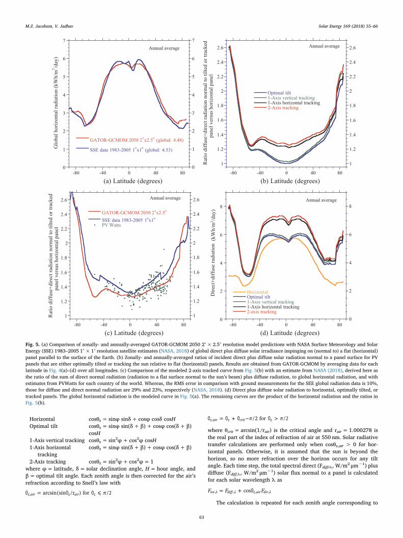
Fig. 5. (a) Comparison of zonally- and annually-averaged GATOR-GCMOM 2050 2°× 2.5° resolution model predictions with NASA Surface Meteorology and SolarEnergy (SSE) 1983–2005 1°× 1° resolution satellite estimates (NASA, 2018) of global direct plus diffuse solar irradiance impinging on (normal to) a flat (horizontal)panel parallel to the surface of the Earth. (b) Zonally- and annually-averaged ratios of incident direct plus diffuse solar radiation normal to a panel surface for PVpanels that are either optimally tilted or tracking the sun relative to flat (horizontal) panels, Results are obtained from GATOR-GCMOM by averaging data for eachlatitude in Fig. 4(a)–(d) over all longitudes. (c) Comparison of the modeled 2-axis tracked curve from Fig. 5(b) with an estimate from NASA (2018), derived here asthe ratio of the sum of direct normal radiation (radiation to a flat surface normal to the sun’s beam) plus diffuse radiation, to global horizontal radiation, and withestimates from PVWatts for each country of the world. Whereas, the RMS error in comparison with ground measurements for the SEE global radiation data is 10%,those for diffuse and direct normal radiation are 29% and 23%, respectively (NASA, 2018). (d) Direct plus diffuse solar radiation to horizontal, optimally tilted, ortracked panels. The global horizontal radiation is the modeled curve in Fig. 5(a). The remaining curves are the product of the horizontal radiation and the ratios inFig. 5(b).

M.Z. Jacobson, V. Jadhav Solar Energy 169 (2018) 55–66

63

each type of panel tilting. Results are summed over all solar wave-lengths and probability intervals (from 170 nm to 10 μm) for each ze-nith angle to get the total flux (Ftot, W/m2) normal to each panel.

Panel output equals the total flux normal to the panel multiplied bythe panel efficiency, the panel loss factor, and the solar cell temperaturecorrection factor. Panel efficiency is the panel’s rated power (W) di-vided by one sun (1000W/m2) and by the panel surface area (m2). Theexample panel used for this study (assuming 2050 panels) has a ratedpower of 390W and surface area of 1.629668m2, giving an efficiencyof 23.93% (Jacobson et al., 2017). This efficiency accounts for the factthat PV cells utilize only a portion of the total solar spectrum.

The panel loss factor equals one minus panel losses (as fractions).Panel losses (not including transmission and distribution losses) areassumed to be a total of 10%, which accounts for soiling (2%), mis-match (2%), wiring (2%), connections (0.5%), light-induced degrada-tion (1.5%), nameplate rating (1%), availability (0.5%) and shading(0.5%) (e.g., NREL, 2017).

The solar cell temperature correction factor is estimated roughly as

= − −C 1 β max(min(T T ,55),0)temp ref c ref

where Tc (K) is the solar cell temperature, βref (K−1) is the temperaturecoefficient, and Tref is the reference temperature. For this study,βref = 0.0025 K−1 and Tref= 298.15 K (Razykov et al., 2011). Althoughβref ranges from 0.0011 to 0.0063, depending on the type of cell(Razykov et al., 2011; Dubey et al., 2013), only one value is used forsimplicity. Another issue with the equation is that it does not accountfor the possible increase in solar cell efficiency for cell temperaturesbelow 298.15 K, which are rare but more relevant at high latitudesduring winter. However, because Ctemp is applied to all panels, re-gardless of tilting or tracking, its value has no impact on the ratio ofincident solar radiation to a tilted or tracked panel to a horizontalpanel. The temperature dependence appears in both the numerator anddenominator of a ratio, thus cancels out.

The solar cell temperature depends on the solar flux and mean windspeed W (m/s) through

= + ∗ + ∗T T 0.32 F /(8.91 2 W)c a tot,

Skoplaki et al. (2008). PV panels are placed in GATOR-GCMOM onrooftops at optimal tilt angles and in utility-scale PV power plants witheither 1-axis vertical tracking, 1-axis horizontal tracking, 2-axistracking, or a combination of all three. For the present study, all threetypes of tracking are assumed to be present in utility PV plants in themodel. The electricity produced by all PV panels in the model is as-sumed ultimately to dissipate as heat, which is released back to the gridcell where the panels exist. Because the PV panels extract solar power,they reduce solar radiation to the rooftop or ground below them,thereby reducing rooftop and ground temperatures. These factors areaccounted for in the model.

Whereas a radiative transfer code (Toon et al., 1989) is used here tocalculate direct and diffuse radiation with different tilting cases, otherstudies have often relied on satellite data combined with geometricequations to estimate radiation to surfaces of different tilting (Breyerand Schmid, 2010a, 2010b; Breyer, 2012; Bogdanov and Breyer, 2016;Kilickaplan et al., 2017; Breyer et al., 2017a, 2017b; Sadiqa et al., 2018;Duffie and Bechman, 2013).

Finally, since GATOR-GCMOM simulates meteorology here in 2050upon transitioning all energy to 100% clean, renewable wind, water,and solar power for all purposes (Jacobson et al., 2017), greenhouse gasmixing ratios in the atmosphere are higher than today, but anthro-pogenic aerosol emissions are virtually zero. Natural aerosol emissionsstill occur.

5. GATOR-GCMOM model results

GATOR-GCMOM was run for the year 2050 at 2.5° W-E×2.0° S-N

horizontal resolution with 68 vertical layers between the ground and0.219 hPa (∼61 km) to estimate the ratios of incident solar flux normalto PV panels with tracking or tilting relative to flat (horizontal) panels.Fig. 3 shows the vertical component of diffuse plus direct downwardradiation impinging on horizontal panels. Whereas the model calculatesboth downward and upward reflected radiation, only the downwardcomponents of direct and diffuse radiation are relevant for radiationimpinging on a horizontal surface. Fig. 5(a) compares 2050 modelpredictions of zonally averaged global (direct plus diffuse) horizontal(parallel to the Earth’s surface) downward radiation with 1983–2005satellite-derived data (NASA, 2018). The uncertainty in the data isgiven as 10%. Considering the coarser resolution of model and thedifference in years, the globally averaged difference between model anddata of only 0.8% is encouraging.

Figs. 4 and 5(b) and (c) show global and zonal ratios of the radiationimpinging normal to tilted or tracked panels relative to horizontal pa-nels. For these calculations, direct solar plus diffuse radiation hittingthe panels are accounted for, but the upward component of ground-reflected radiation is ignored due to the additional complexity of thatcalculation. This omission is likely to affect results primarily at highlatitudes with higher tilt angles. However, the significant benefit oftracking and tilting without accounting for such reflection seen heresuggests that omitting that part of the calculation should have no im-pact on the conclusions of this study.

Fig. 5(b) shows that the benefits of tilting and tracking relative tohorizontal panels generally grow with increasing latitude north or southof the equator. Further, in the global and annual average, 2-axis trackedpanels, 1-axis horizontal tracked panels, 1-axis vertical tracked panels,and optimally tilted panels receive ∼1.39, ∼1.35, ∼1.22, and ∼1.19times the incident solar radiation as do horizontal panels, respectively.As such, on average, 2-axis tracked panels receive 39% more incidentsolar radiation than do horizontal panels and 17% more than do opti-mally tilted panels. However, these ratios vary substantially with lati-tude (Fig. 5(b)).

At virtually all latitudes, 1-axis horizontally tracked panels receivewithin 1–3% the radiation as 2-axis tracked panels (Fig. 5(b)); thus, 1-axis horizontal tracking panels appear more optimal than 2-axistracking panels because, although not calculated here, 1-axis -trackedpanels likely require less land and cost less for the same output as 2-axispanels. Breyer (2012) similarly found that 2-axis tracking did not im-prove solar output much over a specific 1-axis tracking tested therein.1-axis vertical tracking and optimal tilting are less beneficial than 1-axishorizontal or 2-axis tracking. 1-axis horizontal tracking receives muchmore incident solar than does 1-axis vertical tracking below 65° N andS, whereas above 65° N and S, the incident solar is similar for both.

Above 75° N and 60° S, there seems to be little added benefit for anytype of tracking relative to optimal tilting. This result is supportedfurther by results from Breyer (Breyer, 2012). Thus, in the absence ofmore local data and costs, the default recommendation here for utility-scale PV is for 1-axis horizontal tracking for all except the highest la-titudes, where optimal tilting appears sufficient.

Fig. 5(c) compares the ratio of output from 2-axis panels to hor-izontal panels, from Fig. 5(b), with SSE data NASA, 2018 and PVWattscalculations for all countries in Table 1. The SSE curve is derived hereas the sum of direct normal radiation (radiation to a flat surface normalto the sun’s beam) plus diffuse radiation, all divided by global hor-izontal radiation. All three datasets are available from NASA (2018).Whereas, the RMS error in comparison with ground measurements forthe SSE global radiation data is given as 10%, those for diffuse anddirect normal radiation, which are derived from the global radiationdata over 1°× 1° areas, are given as 29% and 23%, respectively. Thegreater uncertainty in the SSE datasets of the diffuse and direct radia-tion than of the global horizontal radiation may explain why the 2-axis-to-horizontal radiation ratios between GATOR-GCMOM and the SSEdata are less similar in Fig. 5(c) than are the global horizontal com-parisons in Fig. 5(a). The fact that the PVWatts results cluster closer to

M.Z. Jacobson, V. Jadhav Solar Energy 169 (2018) 55–66

64

the GATOR-GCMOM model curve further suggests that the GATOR-GCMOM results in Fig. 5(c) may be slightly more accurate than thederived SSE curve.

Finally, Fig. 5(d) shows the annual average direct plus diffuse solarradiation impinging normal to panels of different orientation. Thefigure is obtained by multiplying the ratios in Fig. 5(b) by the modeledglobal horizontal radiation in Fig. 5(a). The significant result of thisfigure is that, over the Antarctic, although horizontal panels receiverelatively little radiation, optimally tilted and tracked panels receivemore sunlight than anywhere else on Earth. This is primarily due to thefacts that the Antarctic receives sunlight 24 h a day in the SouthernHemisphere summer and much of the Antarctic is at a high altitude,thus above more air and clouds than over the Arctic or other latitudes,on average. Tilted and tracked panels over the Arctic receive more ra-diation than between 40° and 80° N, but less than over the Antarctic,due to the lower altitude and greater cloudiness above the surface of theArctic than the Antarctic.

6. Conclusions

In this study, optimal tilt angles for solar panels were first calculatedfor every country of the world using NREL’s PVWatts program. A 3rd-order polynomial fit to the optimal tilt angles as a function of latitudewas developed from the data for the Northern and SouthernHemispheres. This fit appears to give a better fit to PVWatts data above40° N than do previous linear estimates of optimal tilt as a function oflatitude. Whereas, this function and the country-specific optimal tiltangles calculated here are useful for general PV resource analyses, solarinstallers should calculate optimal tilt angles for their specific locationfor greater accuracy.

Optimal tilts found here for all countries were then input into theglobal 3-D GATOR-GCMOM climate model. Radiative transfer calcula-tions were modified to calculate incident radiation normal to optimallytilted, 1-axis vertical tracking (swiveling vertically around a horizontalaxis), 1-axis horizontal tracking (at optimal tilt and swiveling hor-izontally around a vertical axis), and 2-axis tracking panels. Ratios ofincident radiation normal to panels in each of these configurations re-lative to that normal to horizontal panels were calculated worldwide. Inthe global and annual average, these ratios are ∼1.19, ∼1.22, ∼1.35,and ∼1.39, respectively. At virtually all latitudes, 1-axis horizontaltracking receives within 1–3% the incident solar radiation as 2-axistracking. 1-axis horizontal tracking provides much higher solar outputthan does 1-axis vertical tracking below 65° N and S, whereas above 65°N and S, output is similar. There is little added benefit of any type oftracking relative to optimal tilting above 75° N and 60° S. The benefitsof tilting and tracking versus horizontal panels virtually always growwith increasing latitude. Optimally tilted and tracked solar panels overthe Antarctic receive more sunlight than anywhere on Earth, in theannual average.

In sum, when considering only optimal output (not the cost oftracking or land) for a single panel in a utility PV plant, 1-axis hor-izontal tracking is recommended for all except the highest latitudes,where optimal tilting is sufficient. However, final decisions about whatpanel to use also require knowing tracking equipment and land costs,which are not evaluated here.

Cities near the same latitude, such as Calgary, Canada and Beek, theNetherlands, can have vastly different benefits of tilting and trackingrelative to horizontal panels because of the greater aerosol and cloudcover in one (Beek) over the other. An important topic for future re-search is to study how changes in aerosol pollution and resulting cloudcover have affected and will affect global solar radiation incident on PVpanels.

Finally, because tilting and tracking are found to increase incidentsolar radiation at all latitudes, even near the equator, models that donot treat optimal tilting for rooftop PV and tracking for utility PV mayunderestimate significantly country or world PV output.

Acknowledgments

Partial funding for this research was received from the StanfordWoods Institute for the Environment, Innovation Fund Denmark(Renewable Energy Investment Strategies project), the NASA SMDEarth Sciences Division, and the National Science Foundation(Agreement AGS-1441062). Partial computer support came from theNASA high-end computing center.

References

Anderson, J., West, J., 2017. Global cloud cover.< http://eclipsophile.com/global-cloud-cover/> (accessed December 26, 2017).

Bogdanov, D., Breyer, C., 2016. North-east Asian super grid for 100% renewable energysupply: optimal mix of energy technologies for electricity, gas and heat supply op-tions. Energy Convers. Manage. 112, 176–190.

Breyer, C., 2012. Economics of hybrid photovoltaic power plants. Pro Business ISBN: 978-3863863906.

Breyer, C., Schmid, J., 2010. Global distribution of optimal tilt angles for fixed tilted PVsystems. In: 25th EU PVSEC/WCPEC-5. http://dx.doi.org/10.4229/25thEUPVSEC2010-4BV.1.93.

Breyer, C., Schmid, J., 2010. Population density and area weighted solar irradiation:global overview on solar resource conditions for fixed tilted, 1-axis and 2-axes PVsystems. In: 25th EU PVSEC/WCPEC-5. http://dx.doi.org/10.4229/25thEUPVSEC2010-4BV.1.91.

Breyer, C., Bogdanov, D., Aghahosseini, A., Gulagi, A., Child, M., Oyewo, A.S., Farfan, J.,Sadovskaia, K., 2017a. Solar photovoltaics demand for the global energy transition inthe power sector. Prog. Photovoltaics. http://dx.doi.org/10.1002/pip.2950.

Breyer, C., Bogdanov, D., Gulagi, A., Aghahosseini, A., Barbosa, L.S.N.S., Koskinen, O.,Barasa, M., Caldera, U., Afanaseva, S., Child, M., Farfan, J., Vainikka, P., 2017b. Onthe role of solar photovoltaics in global energy transition scenarios. Prog.Photovoltaics 25, 727–745.

Chang, T.P., 2009. The Sun’s apparent position and the optimal tilt angle of a solar col-lector in the northern hemisphere. Sol. Energy 83, 1274–1284.

Chiacchio, M., Ewen, T., Wild, M., Chin, M., Diehl, T., 2011. Decadal variability of aerosoloptical depth in Europe and its relationship to the temporal shift of the North AtlanticOscillation in the realm of dimming and brightening. J. Geophys. Res. 116. http://dx.doi.org/10.1029/2010JD014471.

Dubey, S., Sarvaiya, J.N., Seshadri, B., 2013. Solar photovoltaic (PV) efficiency and itseffect on PV production in the world – a review. Energy Procedia 33, 311–321.

Duffie, J.A., Bechman, W.A., 2013. Solar Engineering of Thermal Process, fourth ed.Wiley, pp. 936.

Gunerhan, H., Hepbash, A., 2009. Determination of the optimal tilt angle of a solar col-lector in the Northern hemisphere. Sol. Energy 83, 1274–1284.

Jacobson, M.Z., 2001a. GATOR-GCMM: a global through urban scale air pollution andweather forecast model. 1. Model design and treatment of subgrid soil, vegetation,roads, rooftops, water, sea ice, and snow. J. Geophys. Res. 106, 5385–5401.

Jacobson, M.Z., 2001b. GATOR-GCMM: 2. A study of day- and nighttime ozone layersaloft, ozone in national parks, and weather during the SARMAP field campaign. J.Geophys. Res. 106, 5403–5420.

Jacobson, M.Z., 2005. A refined method of parameterizing absorption coefficients amongmultiple gases simultaneously from line-by-line data. J. Atmos. Sci. 62, 506–517.

Jacobson, M.Z., 2012. Investigating cloud absorption effects: global absorption propertiesof black carbon, tar balls, and soil dust in clouds and aerosols. J. Geophys. Res. 117,D06205. http://dx.doi.org/10.1029/2011JD017218.

Jacobson, M.Z., Archer, C.L., 2012. Saturation wind power potential and its implicationsfor wind energy. Proc. Nat. Acad. Sci. 109, 15679–15684.

Jacobson, M.Z., Kaufmann, Y.J., Rudich, Y., 2007. Examining feedbacks of aerosols tourban climate with a model that treats 3-D clouds with aerosol inclusions. J. Geophys.Res. 112, D24205. http://dx.doi.org/10.1029/2007JD008922.

Jacobson, M.Z., Archer, C.L., Kempton, W., 2014. Taming hurricanes with arrays of off-shore wind turbines. Nat. Clim. Change 4, 195–200.

Jacobson, M.Z., Delucchi, M.A., Bauer, Z.A.F., Goodman, S.C., Chapman, W.E., Cameron,M.A., Bozonnat, C., Chobadi, L., Clonts, H.A., Enevoldsen, P., Erwin, J.R., Fobi, S.N.,Goldstrom, O.K., Hennessy, E.M., Liu, J., Lo, J., Meyer, C.B., Morris, S.B., Moy, K.R.,O’Neill, P.L., Petkov, I., Redfern, S., Schucker, R., Sontag, M.A., Wang, J., Weiner, E.,Yachanin, A.S., 2017. 100% clean and renewable wind, water, and sunlight (WWS)all-sector energy roadmaps for 139 countries of the world. Joule 1, 108–121(Alphabetical).

Kern, J., Harris, I., 1975. On the optimal tilt of a solar collector. Sol. Energy 17, 97–102.Kilickaplan, A., Bogdanov, D., Peker, B.O., Caldera, U., Aghahosseini, A., Breyer, C., 2017.

An energy transition pathway for Turkey to achieve 100% renewable energy poweredelectricity, desalination and non-energetic industrial gas demand sectors by 2050.Sol. Energy 158, 218–235. http://dx.doi.org/10.1016/j.solener.2017.09.030.

Koronakis, P.S., 1986. On the choice of the angle of tilt for south facing solar collectors inthe Athens basin area. Sol. Energy 36, 217–225.

Lewis, G., 1987. Optimum tilt of a solar collector. Sol. Wind Technol. 4, 407–410.NASA (National Aeronautics and Space Administration), 2018. NASA Langley Research

Center Atmospheric Science Data Center surface meteorology and solar energy (SSE)web portal, Release 6.0.< https://eosweb.larc.nasa.gov/sse/> (accessed March 6,2018).

NREL (National Renewable Energy Laboratory), 2017. PV Watts Calculator. < http://

M.Z. Jacobson, V. Jadhav Solar Energy 169 (2018) 55–66

65

pvwatts.nrel.gov> (accessed November 4, 2017).Ohmura, A., 2009. Observed decadal variations in surface solar radiation and their

causes. J. Geophys. Res. 114. http://dx.doi.org/10.1029/2008JD011290.Pelland, S., Galanis, G., Kallos, G., 2011. Solar and photovoltaic forecasting through post-

processing of the global environmental multiscale numerical weather predictionmodel. Prog. Photovoltaics 21, 284–296.

Razykov, T.M., Ferekides, C.S., Morel, D., Stefanakos, E., Ullal, H.S., Upadhyaya, H.M.,2011. Solar photovoltaic electricity: current status and future prospects. Sol. Energy85, 1580–1608.

Ryberg, D.S., Freeman, J., Blair, N., 2015. Quantifying interannual variability for pho-tovoltaic systems in PVWatts. National Renewable Energy Laboratory.< https://www.nrel.gov/docs/fy16osti/64880.pdf > .

Sadiqa, A., Gulagi, A., Breyer, C., 2018. Energy transition roadmap towards 100% re-newable energy and role of storage technologies for Pakistan by 2050. J. Energy 147,

518–533. http://dx.doi.org/10.1016/j.energy.2018.01.027.Skoplaki, E., Boudouvis, A.G., Palyvos, J.A., 2008. A simple correlation for the operating

temperature of photovoltaic modules of arbitrary mounting. Sol. Energy Mater. Sol.Cells 92, 1393–1402.

Talebizadeh, P., Mehrabian, M.A., Abdolzadeh, M., 2011. Determination of optimumslope angles of solar collectors based on new correlations. Energy Sources Part A 33,1567–1580.

The World Bank, 2017. PM2.5 air pollution, mean annual exposure.< https://data.worldbank.org/indicator/EN.ATM.PM25.MC.M3> (accessed December 26, 2017).

Toon, O.B., McKay, C.P., Ackerman, T.P., 1989. Rapid calculation of radiative heatingrates and photodissociation rates in inhomogeneous multiple scattering atmospheres.J. Geophys. Res. 94 (16), 287–301.

Yadav, A.K., Chandel, S.S., 2013. Tilt angle optimization to maximize incident solar ra-diation: a review. Renew. Sustain. Energy Rev. 23, 503–513.

M.Z. Jacobson, V. Jadhav Solar Energy 169 (2018) 55–66

66