WORKSHEET: Adjustment Case Studies

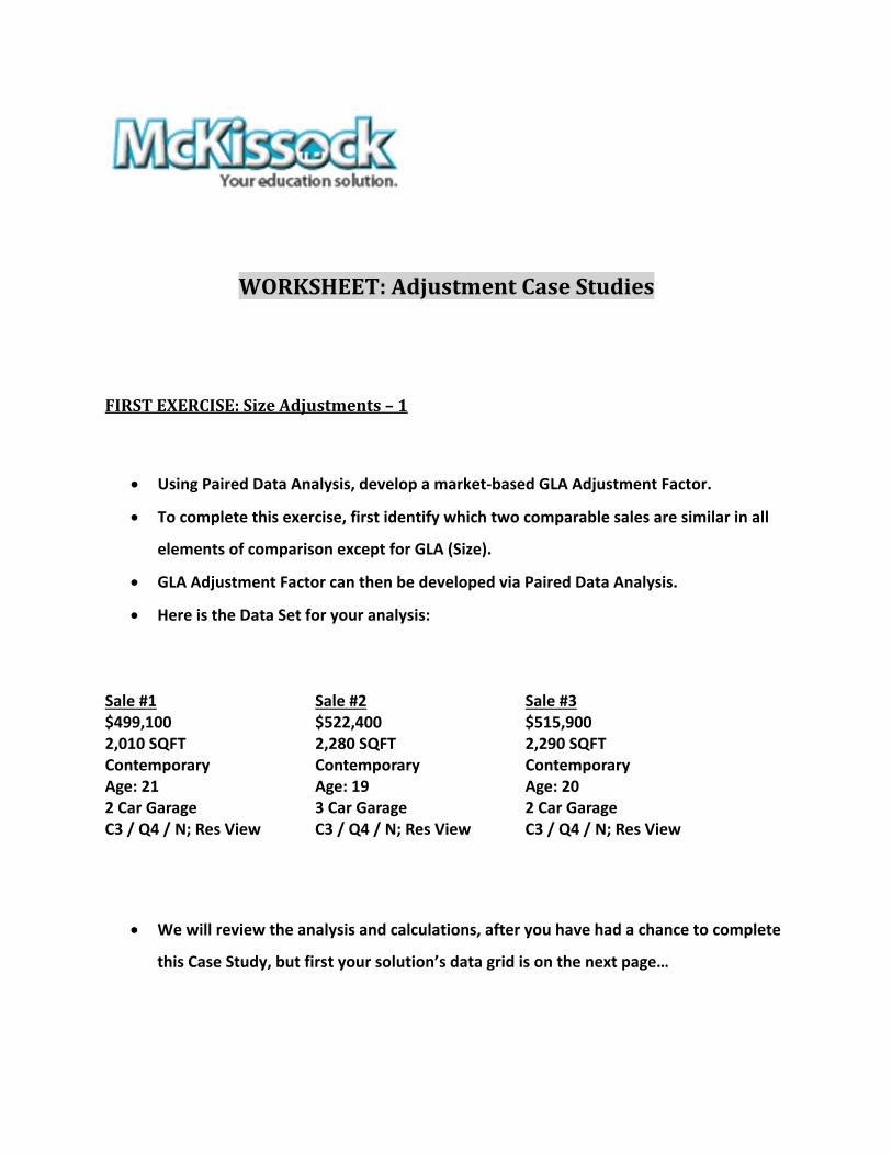
WORKSHEET:AdjustmentCaseStudies

FIRSTEXERCISE:SizeAdjustments–1

Using Paired Data Analysis, develop a market‐based GLA Adjustment Factor.

To complete this exercise, first identify which two comparable sales are similar in all

elements of comparison except for GLA (Size).

GLA Adjustment Factor can then be developed via Paired Data Analysis.

Here is the Data Set for your analysis:

Sale #1 Sale #2 Sale #3 $499,100 $522,400 $515,900 2,010 SQFT 2,280 SQFT 2,290 SQFT Contemporary Contemporary Contemporary Age: 21 Age: 19 Age: 20 2 Car Garage 3 Car Garage 2 Car Garage C3 / Q4 / N; Res View C3 / Q4 / N; Res View C3 / Q4 / N; Res View

We will review the analysis and calculations, after you have had a chance to complete

this Case Study, but first your solution’s data grid is on the next page…

FIRSTEXERCISE:SizeAdjustments–2

SolutionDataGrid

Element SALE#___ DIFFERENCE SALE#___

SalesPrice $______,______ $___,______* $______,______

GLA __,______ ______* __,______

Design/Style Contemporary Contemporary

Age ______ ______

Garage 2CarGarage 2CarGarage

Cdtn/Qlty/View C3/Q4/N;Res C3/Q4/N;Res

HINTS:

1. Selectthetwocomparablesalestobeusedinpaireddataanalysis.

2. Entertheirmissinginformationinthehighlighted________fields.

3. CalculatethedifferencesinsalespricesandinGLAbetweenthecomparables

4. $___,______*/______*=$_____perSquareFootGLAAdjustment.

SECONDEXERCISE:BedroomAdjustments–1

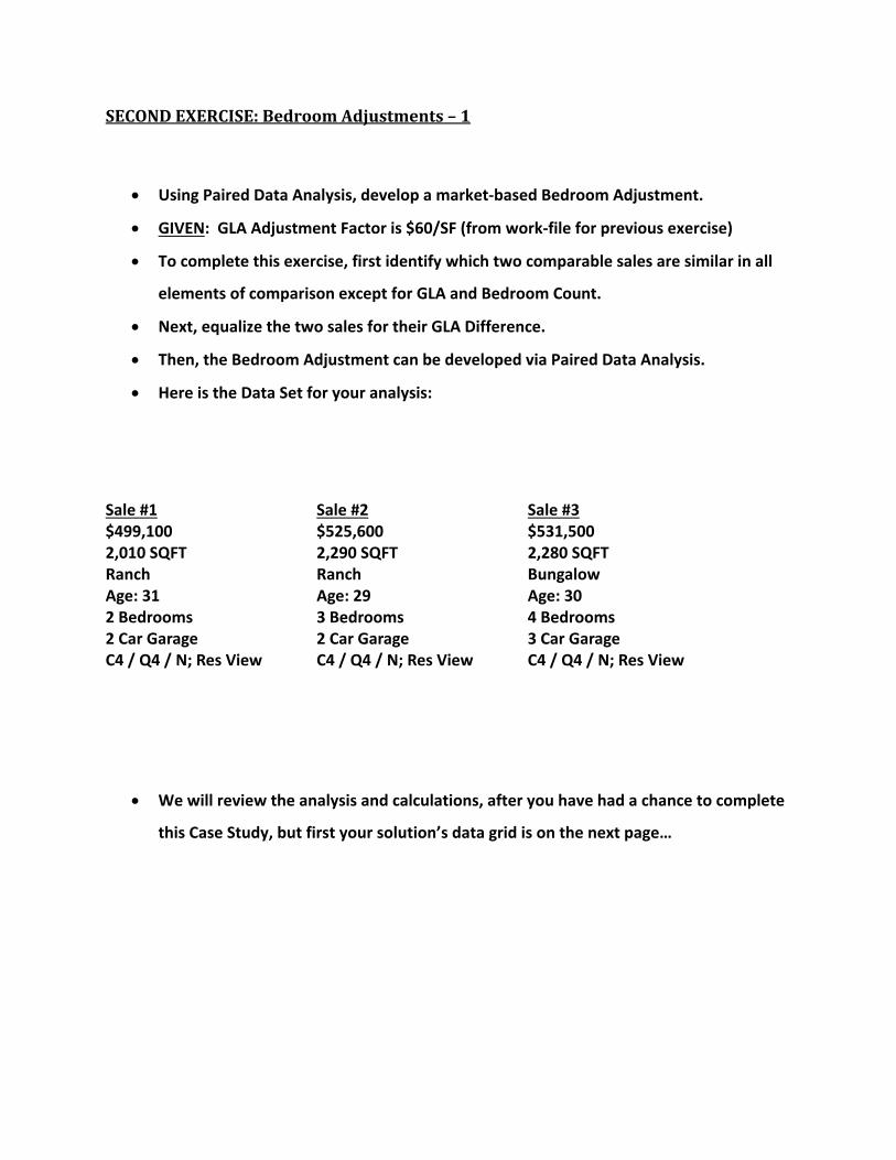
Using Paired Data Analysis, develop a market‐based Bedroom Adjustment.

GIVEN: GLA Adjustment Factor is $60/SF (from work‐file for previous exercise)

To complete this exercise, first identify which two comparable sales are similar in all

elements of comparison except for GLA and Bedroom Count.

Next, equalize the two sales for their GLA Difference.

Then, the Bedroom Adjustment can be developed via Paired Data Analysis.

Here is the Data Set for your analysis:

Sale #1 Sale #2 Sale #3 $499,100 $525,600 $531,500 2,010 SQFT 2,290 SQFT 2,280 SQFT Ranch Ranch Bungalow Age: 31 Age: 29 Age: 30 2 Bedrooms 3 Bedrooms 4 Bedrooms 2 Car Garage 2 Car Garage 3 Car Garage C4 / Q4 / N; Res View C4 / Q4 / N; Res View C4 / Q4 / N; Res View

We will review the analysis and calculations, after you have had a chance to complete

this Case Study, but first your solution’s data grid is on the next page…

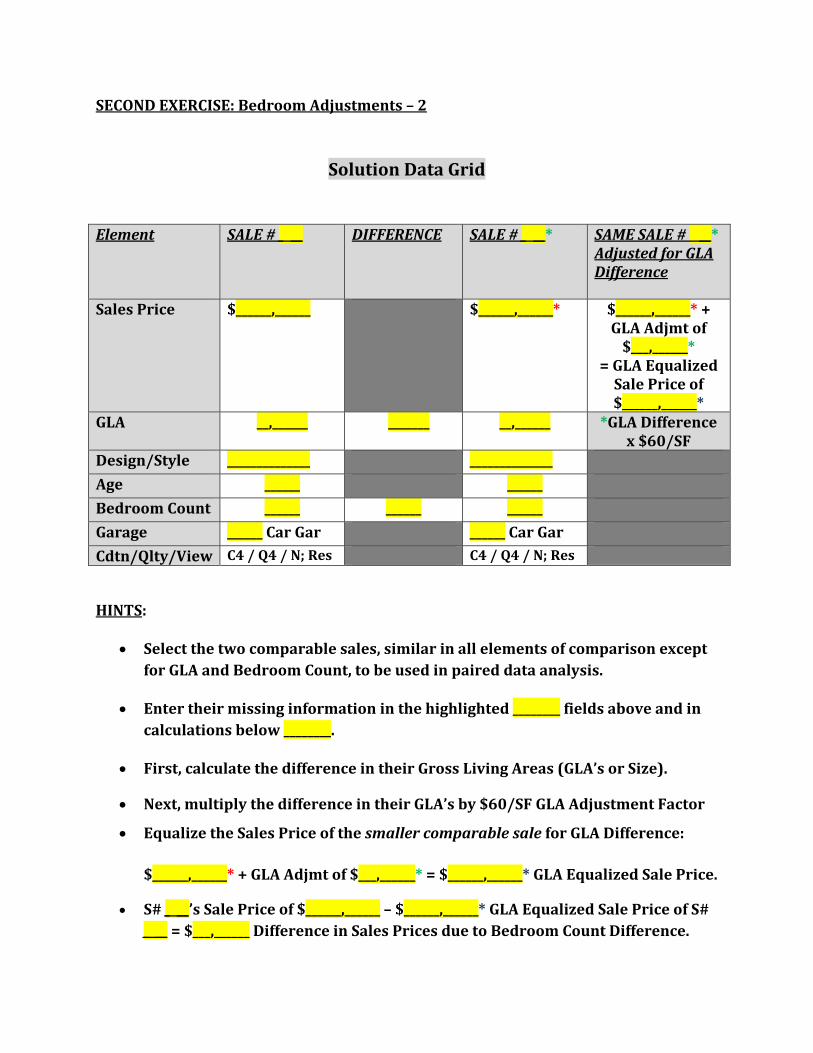
SECONDEXERCISE:BedroomAdjustments–2

SolutionDataGrid

Element SALE#___ DIFFERENCE SALE#___* SAMESALE#__*AdjustedforGLADifference

SalesPrice $______,______ $______,______* $______,______*+GLAAdjmtof$___,______*

=GLAEqualizedSalePriceof$______,______*

GLA __,______ _______ __,______ *GLADifferencex$60/SF

Design/Style ______________ ______________

Age ______ ______

BedroomCount ______ ______ ______

Garage ______CarGar ______CarGar


HINTS:

Selectthetwocomparablesales,similarinallelementsofcomparisonexceptforGLAandBedroomCount,tobeusedinpaireddataanalysis.

Entertheirmissinginformationinthehighlighted________fieldsaboveandincalculationsbelow________.

First,calculatethedifferenceintheirGrossLivingAreas(GLA’sorSize).

Next,multiplythedifferenceintheirGLA’sby$60/SFGLAAdjustmentFactor

EqualizetheSalesPriceofthesmallercomparablesaleforGLADifference:

$______,______*+GLAAdjmtof$___,______*=$______,______*GLAEqualizedSalePrice.

S#___’sSalePriceof$______,______–$______,______*GLAEqualizedSalePriceofS#___=$___,______DifferenceinSalesPricesduetoBedroomCountDifference.

THIRDEXERCISE:BathroomAdjustments–1

Using Income Capitalization, develop a market‐based Bathroom Adjustment Factor.

To complete this exercise, first finish calculating the Gross Rent Multipliers (GRM’s) in

the first data table below by filling in highlighted blanks.

Then, reconcile the Range of Gross Rent Multipliers (GRM’s) to select an appropriate

GRM.

Next, research Rental Units with 1.0 vs. 2.0 Bathrooms to identify the Difference in

Rental Income.

Capitalize the Difference in Rental Income for 1 Bathroom vs. 2 Bathroom Units to

develop a market‐based Bathroom Adjustment.

Here are the Data Sets for your analysis:

Sales Price S#1: $389,400 S#2: $401,900 S#3: $434,900

Monthly Rent $2,250 $2,300 $2,500

Sale$ Price/Rent 389,400/2,250 401,900/_,___ ___,___/_,___

GRM 173 ~ ___ ~ ___ ~

GRM Reconciliation: A GRM of ___ is selected.

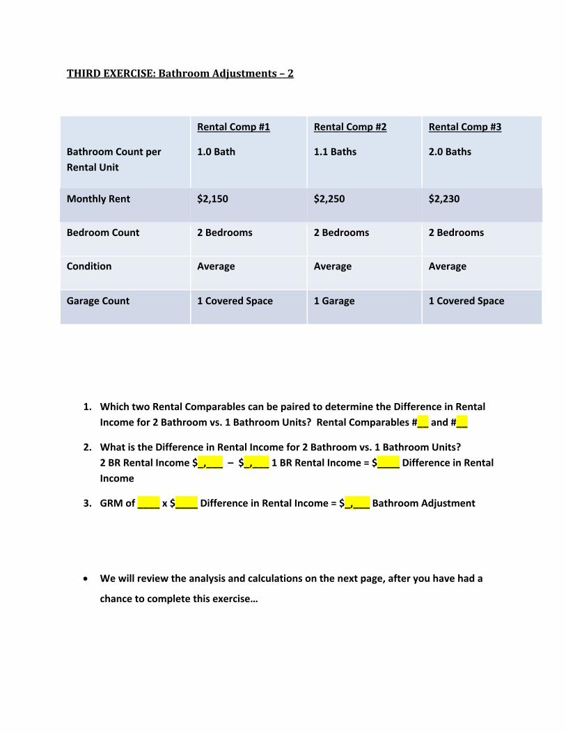
THIRDEXERCISE:BathroomAdjustments–2

Bathroom Count per

Rental Unit

Rental Comp #1

1.0 Bath

Rental Comp #2

1.1 Baths

Rental Comp #3

2.0 Baths

Monthly Rent $2,150 $2,250 $2,230

Bedroom Count 2 Bedrooms 2 Bedrooms 2 Bedrooms

Condition Average Average Average

Garage Count 1 Covered Space 1 Garage 1 Covered Space

1. Which two Rental Comparables can be paired to determine the Difference in Rental

Income for 2 Bathroom vs. 1 Bathroom Units? Rental Comparables #__ and #__

2. What is the Difference in Rental Income for 2 Bathroom vs. 1 Bathroom Units?

2 BR Rental Income $_,___ – $_,___ 1 BR Rental Income = $____ Difference in Rental

Income

3. GRM of ____ x $____ Difference in Rental Income = $_,___ Bathroom Adjustment

We will review the analysis and calculations on the next page, after you have had a

chance to complete this exercise…

FOURTHEXERCISE:(ChangingMarketConditionsover)TimeAdjustments

Using a Sale and Resale of the Same Property, where the only significant difference is

the time of sale, develop a market‐based Time Adjustment.

First, complete the data table below by filling in highlighted blanks.

Next, calculate the Percentage Difference in the two Sales Prices with this formula:

2nd Sale Price – 1st Sale Price / 1st Sale Price = % Difference in Sales Prices*

Sales Price Date of Sale

(Contract)

% of Sales

Price Change

Months

Elapsed

% of Time Adjustment

per Month

$314,900 02/12/2015 N/A N/A N/A

$336,500 03/14/2016 _.___%* ___ Months _.___%* / ___ Months =

_.___% ~ per Month

Then, count the Months Elapsed between the two Contract Sales Dates.

Finally, divide the % of Sales Price Change by the Number of Months Elapsed to

calculate the % of Time Adjustment per Month.

We will review the analysis and calculations on the next page, after you have had a


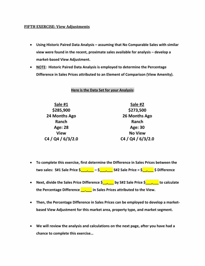
FIFTHEXERCISE:ViewAdjustments

Using Historic Paired Data Analysis – assuming that No Comparable Sales with similar

view were found in the recent, proximate sales available for analysis – develop a

market‐based View Adjustment.

NOTE: Historic Paired Data Analysis is employed to determine the Percentage

Difference in Sales Prices attributed to an Element of Comparison (View Amenity).

Here is the Data Set for your Analysis:

• To complete this exercise, first determine the Difference in Sales Prices between the

two sales: S#1 Sale Price $___,___ – $___,___ S#2 Sale Price = $__,___ $ Difference

• Next, divide the Sales Price Difference $__,___ by S#2 Sale Price $___,___ to calculate

the Percentage Difference __.___ in Sales Prices attributed to the View.

• Then, the Percentage Difference in Sales Prices can be employed to develop a market‐

based View Adjustment for this market area, property type, and market segment.

• We will review the analysis and calculations on the next page, after you have had a


Sale #1 $285,900

24 Months Ago Ranch Age: 28 View

C4 / Q4 / 6/3/2.0

Sale #2

$273,500

26 Months Ago

Ranch

Age: 30

No View

C4 / Q4 / 6/3/2.0

FIRSTEXERCISESOLUTION:SizeAdjustments

Element SALE#_3_ DIFFERENCE SALE#_1_

SalesPrice $515,900 $16,800* $499,100

GLA 2,290SF 280*SF 2,010SF

Design/Style Contemporary Contemporary

Age 20 21

Garage 2CarGarage 2CarGarage


Comparable Sales #3 and #1 are employed in this Paired Data Analysis

First, calculate the difference in their Sales Prices:

Sale #3’s Sale Price $515,900 ‐ $499,100 Sale #1’s Sale Price = $16,800*

Next, calculate the difference in their Gross Living Areas (GLA, or Size)

Sale #3’s GLA ‐ Sale #1’s GLA = 280*

Finally, divide the difference in their Sales Prices by the difference in their GLA’s

$16,800* / 280* SF = $60 per Square Foot GLA Adjustment.

Price‐per‐Square‐Foot solution is the current market‐based GLA Adjustment Factor, in

this market, for this property type, and market segment:

GLA Adjustment = $60/SF

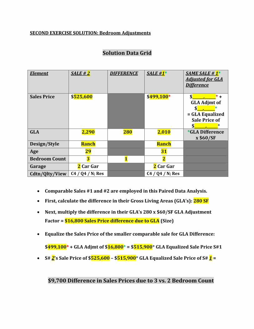
SECONDEXERCISESOLUTION:BedroomAdjustments

SolutionDataGrid

Element SALE#2 DIFFERENCE SALE#1* SAMESALE#1*AdjustedforGLADifference

SalesPrice $525,600 $499,100* $______,______*+GLAAdjmtof$___,______*

=GLAEqualizedSalePriceof$______,______*

GLA 2,290 280 2,010 *GLADifferencex$60/SF

Design/Style Ranch Ranch

Age 29 31

BedroomCount 3 1 2

Garage 2CarGar 2CarGar


ComparableSales#1and#2areemployedinthisPairedDataAnalysis.

First,calculatethedifferenceintheirGrossLivingAreas(GLA’s):280SF

Next,multiplythedifferenceintheirGLA’s280x$60/SFGLAAdjustment

Factor=$16,800SalesPricedifferenceduetoGLA(Size)

EqualizetheSalesPriceofthesmallercomparablesaleforGLADifference:

$499,100*+GLAAdjmtof$16,800*=$515,900*GLAEqualizedSalePriceS#1

S#2’sSalePriceof$525,600–$515,900*GLAEqualizedSalePriceofS#1=

$9,700DifferenceinSalesPricesdueto3vs.2BedroomCount

THIRDEXERCISESOLUTION:BathroomAdjustments

Here are the completed Gross Rent Multiplier (GRM) calculations for the data table:

Sales Price S#1: $389,400 S#2: $401,900 S#3: $434,900

Monthly Rent $2,250 $2,300 $2,500

Sale$ Price/Rent 389,400/2,250 401,900/2,300 434,900/2,500

GRM 173 ~ 175 ~ 174 ~

GRM Reconciliation: A GRM of 174 is selected.

1. Which two Rental Comparables can be paired to determine the Difference in Rental

Income for 2 Bathroom vs. 1 Bathroom Units? Rental Comparables #3 and #1

2. What is the Difference in Rental Income for 2 Bathroom vs. 1 Bathroom Units?

2 BR Rental Income $2,230 – $2,150 1 BR Rental Income = $80 Difference in Rental

Income

3. GRM of 174 x $80 Difference in Rental Income = $13,900 ~ Bathroom Adjustment

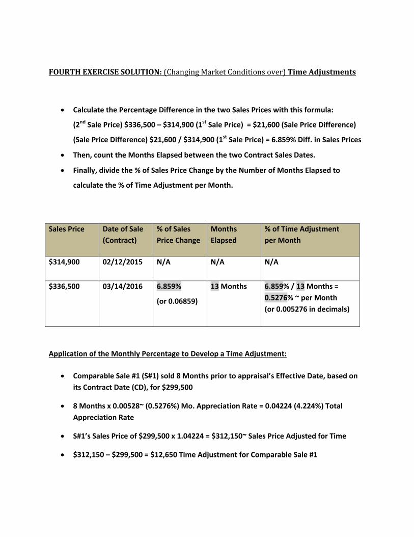
FOURTHEXERCISESOLUTION:(ChangingMarketConditionsover)TimeAdjustments

Calculate the Percentage Difference in the two Sales Prices with this formula:

(2nd Sale Price) $336,500 – $314,900 (1st Sale Price) = $21,600 (Sale Price Difference)

(Sale Price Difference) $21,600 / $314,900 (1st Sale Price) = 6.859% Diff. in Sales Prices

Then, count the Months Elapsed between the two Contract Sales Dates.

Finally, divide the % of Sales Price Change by the Number of Months Elapsed to

calculate the % of Time Adjustment per Month.

Sales Price Date of Sale

(Contract)

% of Sales

Price Change

Months

Elapsed

% of Time Adjustment

per Month

$314,900 02/12/2015 N/A N/A N/A

$336,500 03/14/2016 6.859%

(or 0.06859)

13 Months 6.859% / 13 Months =

0.5276% ~ per Month

(or 0.005276 in decimals)

Application of the Monthly Percentage to Develop a Time Adjustment:

Comparable Sale #1 (S#1) sold 8 Months prior to appraisal’s Effective Date, based on

its Contract Date (CD), for $299,500

8 Months x 0.00528~ (0.5276%) Mo. Appreciation Rate = 0.04224 (4.224%) Total

Appreciation Rate

S#1’s Sales Price of $299,500 x 1.04224 = $312,150~ Sales Price Adjusted for Time

$312,150 – $299,500 = $12,650 Time Adjustment for Comparable Sale #1

FIFTHEXERCISESOLUTION:ViewAdjustments

Here is the Data Set for your Analysis:

• Determine the Difference in Sales Prices between the two sales:

S#1 Sale Price $285,900 – $273,500 S#2 Sale Price = $12,400 Sales Price Difference

• Next, divide the Sales Price Difference $12,400 by S#2 Sale Price $273,500 to calculate

the Percentage Difference 4.534% (or 0.045338 in decimals) in Sales Prices Attributed

to the View.

Application of the % Difference in Historic Sales Prices to Develop a View Adjustment:

• Comparable Sale #3 (S#3), which has an Inferior neutral View when compared to the Subject’s Superior View Amenity, sold for $299,500

• S#3’s Sales Price of $299,500 x 0.04534 (4.534%) Percentage of Sale Price Attributed to the View = $13,579 ($13,500~) View Adjustment

• S#3 is Adjusted +$13,500 for its Inferior View

Sale #1 $285,900

24 Months Ago Ranch Age: 28 View

C4 / Q4 / 6/3/2.0

Sale #2

$273,500

26 Months Ago

Ranch

Age: 30

No View

C4 / Q4 / 6/3/2.0

WORKSHEET: Adjustment Case Studies

Documents

Transcript of WORKSHEET: Adjustment Case Studies