Workload Models and Performance Evaluation of Cloud...

.

Workload Models and Performance

Evaluation of Cloud Storage Services

RT.DCC.003/2015

Glauber D. Gonçalves

Idilio Drago

Alex Borges Vieira

Ana Paula Couto da Silva

Jussara Marques de Almeida

Marco Mellia

OUTUBRO

2015

UFMG - ICEX DEPARTAMENTO DE CIÊNCIA DA

C O M P U T A Ç Ã O UNIVERSIDADE FEDERAL DE MINAS GERAIS

Workload Models and Performance Evaluation of

Cloud Storage Services

Glauber D. Goncalvesa,∗, Idilio Dragob, Alex B. Vieirac, Ana Paula Couto daSilvaa, Jussara M. Almeidaa, Marco Melliab

aUniversidade Federal de Minas Gerais, BrazilbPolitecnico di Torino, Italy

cUniversidade Federal de Juiz de Fora, Brazil

Abstract

Cloud storage systems are currently very popular with many companies offeringservices, including worldwide providers such as Dropbox, Microsoft and Google.These companies as well as providers entering the market could greatly benefitfrom a deep understanding of typical workload patterns their services have toface in order to develop cost-effective solutions. Yet, despite recent studies ofusage and performance of these systems, the underlying processes that generateworkload to the system have not been deeply studied.

This paper presents a thorough investigation of the workload generated byDropbox customers. We propose a hierarchical model that captures user ses-sions, file system modifications and content sharing patterns. We parameter-ize our model using passive measurements gathered from 4 different networks.Next, we use the proposed model to drive the development of CloudGen, a newsynthetic workload generator that allows the simulation of the network traf-fic created by cloud storage services in various realistic scenarios. We validateCloudGen by comparing synthetic traces with actual data from operationalnetworks. We then show its applicability by investigating the impact of thecontinuing growth in cloud storage popularity on bandwidth consumption. Ourresults indicate that a hypothetical 4-fold increase in both user population andcontent sharing could lead to 30 times more network traffic. CloudGen is avaluable tool for administrators and developers interested in engineering anddeploying cloud storage services.

Keywords: Cloud Storage, Models, Measurements

∗Corresponding authorEmail addresses: [email protected] (Glauber D. Goncalves),

[email protected] (Idilio Drago), [email protected] (Alex B. Vieira),[email protected]; (Ana Paula Couto da Silva), [email protected] (JussaraM. Almeida), [email protected] (Marco Mellia)

Preprint submitted to Computer Networks October 1, 2015

1. Introduction

Cloud storage is a data-intensive Internet service that synchronizes files withthe cloud and among different end user devices, such as PCs, tablets and smart-phones. It offers the means for customers to easily backup data and to performcollaborative work, with files being automatically uploaded and synchronized.Cloud storage is already one of the most popular Internet services, generatinga significant amount of traffic [1]. Well-established players such as Dropbox, aswell as giants like Google and Microsoft, face a fierce competition for customers.Currently, Dropbox leads the market with more than 400 million users by 2015,1

and Google and Microsoft show a fast growth [2], thanks to solutions that aremore and more integrated into Windows or Android Operating Systems.

Both established and new players could greatly benefit from a deep under-standing of the workload patterns that cloud storage services have to face inorder to develop cost-effective solutions. However, several aspects make theanalysis of cloud storage workloads a challenge. As the stored content is privateand synchronization protocols are mostly proprietary, the knowledge of howthese systems work is limited outside companies running the services. It is thusvery hard to obtain large scale data that could drive workload analyses, givenalso the widespread use of encryption for both data and control messages [3].

Indeed, we are aware of only a few recent efforts to analyze the characteristicsof cloud storage services [1], focusing either on architectural design aspects [4, 5],quality of experience [6, 7], or benchmark-driven performance studies [3, 8, 9].Yet, a characterization of the underlying client processes that generate workloadto the system, notably the data transfer patterns that emerge from such pro-cesses, is only partly addressed by our preliminary efforts presented in [10, 11].Such knowledge is key to analyze the impact of these services on network band-width requirements as well as to the design of future services.

Towards filling this gap, this paper performs a thorough investigation of theworkload experienced by Dropbox, the currently most popular cloud storageservice. We propose a hierarchical model that describes client behavior in suc-cessive Dropbox sessions. Within each session, our model captures file systemmodifications and content sharing among users and devices, as well as clientinteractions with Dropbox servers while storing and retrieving files. We param-eterize the model based on the analysis of Dropbox traffic traces collected infour different networks, namely two university networks – one in South Americaand one in Europe, and two European Internet Service Provider (ISP) networks.We offer these traces to the community, to foster future studies.

Next, we use the model to drive the development of a new synthetic work-load generator, called CloudGen. Our validation experiments, comparing realand synthetic workloads, show that CloudGen is able to reproduce the behaviorof Dropbox customers. CloudGen is a valuable tool that allows network ad-ministrators and cloud storage developers to analyze the traffic volume of cloud

1https://www.dropbox.com/news/company-info

2

https://www.dropbox.com/news/company-info

storage as well as to evaluate future system optimization and developments invarious synthetic, but still realistic, workload scenarios.

Given the steady increase in Dropbox user base [12], we illustrate the appli-cability of CloudGen by evaluating how network traffic would change in edgenetworks, such as ISP and campus networks, when customer population growsand when users share more content via cloud storage. Our results suggest thata hypothetical 4-fold increase in both user population and content sharing couldlead to 30 times more cloud storage traffic, eventually challenging the capacityof such systems.

In sum, our main contributions are the following:

• We propose a hierarchical model of the Dropbox client behavior and pa-rameterize it using passive measurements gathered from 4 different net-works. To the best of our knowledge, we are the first to model the clientbehavior and data sharing in Dropbox.

• We develop and validate a synthetic workload generator (CloudGen) thatreproduces user sessions, traffic volume and data sharing patterns. Weoffer CloudGen as free software to the community.2

• We illustrate the applicability of CloudGen in a case study, where theimpact of larger user populations and more content sharing are explored.

This paper extends our previous efforts to model Dropbox client behav-ior [10, 11]. Specifically, unlike in [10], our new model explicitly captures datasharing and modifications. We also build on top of the proposed model bydeveloping and validating a new workload generator, which was introduced inour preliminary work in [11], and we use the workload generator to analyze thenetwork traffic of cloud storage services in hypothetical future scenarios.

The paper is organized as follows. Section 2 presents the background onDropbox. Our data collection methodology is presented in Section 3. Section 4describes our client behavior model and characterizes its components, whereasour workload generator is introduced in Section 5. We illustrate CloudGenapplicability in Section 6, exploring possible future scenarios for cloud storageusage. Section 7 reviews related work, while Section 8 summarizes our contri-butions and lists future work. Finally, additional details of the characterizationof our model components are provided in Appendix A.

2. Overview of Dropbox

2.1. Architecture

Dropbox relies on thousands of servers that are split into two major groups:control and storage servers. Control servers are responsible for: (i) user authen-tication; (ii) management of the Dropbox file system metadata; and (iii) man-

2CloudGen is available at http://cloudgen.sourceforge.net.

3

http://cloudgen.sourceforge.net

agement of device sessions. Storage servers are in charge of the actual storageof data, and are outsourced to the Amazon cloud by the time of writing.

Users can link several devices to Dropbox using both PC and mobile clients.Web interfaces are also available, providing an easy way to access files in thecloud. We focus only on PC clients in this work, since they are responsible formost workload in cloud storage [1], although our model and workload generatorcan be trivially extended to other usage scenarios as well.

Every user registered with Dropbox is assigned a unique user ID. Every timeDropbox is installed on a PC, it provides the PC a unique device ID. Users needto select an initial folder in their PCs from where files are kept synchronizedwith the remote Dropbox servers. Users might decide to share content withother users. This is achieved by selecting a particular folder that is shown toevery participant in the sharing as a shared folder.

Internally, Dropbox treats the initial folders selected at configuration timeand all shared folders indistinctly. They are all called namespaces, and eachis identified by a unique namespace ID. Namespaces are usually synchronizedwith all devices of the user and, for shared folders, with all devices of all usersparticipating in the sharing. Each namespace is also attached to a monotonicjournal ID (JID), representing the namespace latest version [13].

We refer the reader to [1] for details of the architecture of Dropbox.

2.2. Client Protocols

Our work takes as reference the protocols used by Dropbox in its clientv2.8.4.3 A device connecting to Dropbox contacts control servers to performuser authentication and to send its list of namespaces and respective journalIDs. This step allows servers to decide whether the device is updated or if itneeds to be synchronized. If outdated, the device executes storage operations(exemplified next), until it becomes synchronized with the cloud. After that,the device finishes the initial synchronization phase and enters in steady state.

When a Dropbox device identifies new local changes (e.g., new files, or filemodifications), it starts a synchronization cycle. The device first performs sev-eral local operations to prepare files for synchronization. For example, Dropboxsplits files in chunks of up to 4 MB and calculates content hashes for each ofthem. Chunks are compressed locally, and they might be grouped into bundlesto improve performance [3].

As soon as chunks/bundles are ready for transmission, the device behaves asdepicted in Figure 1a. It first contacts a Dropbox control node, sending a list ofnew chunk hashes – see the commit request in the left-hand side of Figure 1a.The servers answer with the subset of hashes that is not yet uploaded (see needblocks (nb) reply). Note that servers can skip requesting chunks it already has,a mechanism known as client-side deduplication [14]. If any hash is unknown toservers, the device executes several storage operations directly with the storage

3Note that our model is applicable to other cloud storage systems and Dropbox versionsas well. See [3] for a comparison of different cloud storage designs.

4

Control

Storage

Device A Timecommit[1,2,3]

nb[1,2,3]

store[1]

ok

store[2,3]

ok

commit[1,2,3]

nb[]

(a) Control and Storage Protocols

NotificationServer

Device A Timesubscribe subscribe subscribe

punt punt new

Heartbeat (≈ 60s) Heartbeat (≈ 60s) Asynchronous

(b) Notification Protocol

Figure 1: Basic operation of Dropbox client protocols.

servers (see store requests).4 Finally, the device contacts again the Dropboxcontrol node, repeating the initial procedure to complete the transaction.

Since the login and until going off-line, devices keep open a connection witha Dropbox control server, which we call notification server. Notification serversare in charge of spreading information about changes performed in namespaces.For instance, when a partner in a shared folder performs changes, notificationsare sent to all devices participating in the sharing. Devices then contact theDropbox storage and control centers to retrieve updates.

The notification protocol is illustrated in Figure 1b. As soon as a deviceconnects to Dropbox, it contacts a notification server (see subscribe request).Contrary to other Dropbox communications that have always been performedover SSL/TLS, the traffic to notification servers used to be exchanged in plaintext HTTP during the period our datasets were collected. Every message sentto notification servers contains a device ID and a user ID, as well as the full listof namespaces in the client with their repetitive journal IDs.

Notification servers answer after approximately 60 s if no changes in names-paces are performed in the meanwhile (see punt reply). The arrival of an answertriggers the client to resend a subscribe request, thus acting like a heartbeat pro-tocol. If any changes are detected in a namespace, the servers instead answerto the pending request asynchronously, with a new message. The client thenreacts to the notification, starting a new synchronization as in Figure 1a.

4Dropbox also deploys a protocol for synchronizing devices in Local Area Networks, calledLAN Sync. Devices in a LAN can use it to exchange files without retrieving content from thecloud. Since such traffic does not travel outside the LAN, we ignore the effects of LAN Sync.

5

Table 1: Overview of our datasets.

Name DevicesUpload(TB)

Download(TB)

Namespaces Changes1 Period

Campus-1 12,587 1.7 3.8 10,609 2,690,617 04/14–06/14

Campus-2 1,987 0.6 1.0 9,861 507,394 04/14–06/14

PoP-1 9,478 3.9 6.8 28,899 1,657,744 10/13–04/14

PoP-2 3,376 2.4 3.7 12,050 1,306,045 07/13–05/14

Total 27,428 8.6 15.3 61,418 6,161,800 –1 Number of times the journal ID of a namespace has changed.

By observing traffic to notification servers, it is possible to identify wheneach namespace is changed. We explore these messages to trace the evolutionof namespaces of Dropbox clients and reconstruct client behavior.

3. Datasets and Methodology

3.1. Datasets

We rely on Tstat [15] to perform passive measurements and collect datarelated to Dropbox from different networks. Tstat monitors each TCP con-nection, exposing flow level information, including: (i) anonymized client IPaddresses; (ii) timestamps of the first and the last packets with payload in eachflow; (iii) the amount of exchanged data; and (iv) the Fully Qualified DomainName (FQDN) the client resolved via DNS queries prior to open the flow [16].

We adopt a methodology similar to the one in [1] to filter and classify Drop-box traffic. Specifically, we take advantage of the FQDNs exported by Tstatto filter records related to the several Dropbox servers. For example, we iso-late flow records related to the storage of data by looking for FQDNs contain-ing dl-client*.dropbox.com. Similarly, we use notify*.dropbox.com to filter flowrecords associated with the notification of changes and heartbeat messages.

In addition to TCP level flows, we use the HTTP monitoring plug-in of Tstatto export, simultaneously to the flows, information seen in heartbeat messages(see Section 2.2). For each event, we gather: (i) the timestamp of the event;(ii) the device ID related to the event; (iii) the user ID related to the event;(iv) each namespace ID registered in the device; and (v) the latest journal IDof each namespace.5

We have collected traffic in 4 different networks, including University cam-puses and ISP networks. Table 1 summarizes our datasets, presenting the num-ber of Dropbox devices, the Dropbox traffic volume, the number of uniquenamespaces, the number of times the journal ID of a namespace has changed,and the data capture period.

5Our data does not include any information that could reveal user identities, or informationabout the content users store in Dropbox. IP addresses are anonymized directly in the probes,whereas all Dropbox IDs are numeric keys that offer no hints about users’ identities.

6

Campus-1 and Campus-2 datasets have been collected at border routersof two distinct campus networks. Campus-1 includes traffic of a large SouthAmerican university with user population (including faculty, student and staff)of ≈ 57, 000 people. Campus-2 serves around ≈ 15, 000 users in a European uni-versity. Both datasets include traffic generated by wired workstations in researchand administrative offices, whereas Campus-1 includes also WiFi networks.

PoP-1 and PoP-2 have been collected at distinct Points of Presence (PoPs)of a European ISP, aggregating more than 25, 000 and 5, 000 households, re-spectively. ADSL lines provide access to 80% of the users in PoP-1, while FiberTo The Home (FTTH) is available to the remaining 20% of users in PoP-1 andto all users in PoP-2. Ethernet and/or WiFi are used at home to connect endusers’ devices, such as PCs or smartphones.

In total, we have observed more than 20 TB of data exchanges with Drop-box servers, 27 k unique Dropbox devices and 61 k unique namespaces duringapproximately 1 year of data collections. Our datasets provide not only a large-scale view in terms of number of users/devices, but also a rich and longitudinalpicture of the Dropbox usage. A key contribution of our work is the release ofanonymized data to the public, aiming to foster new researches and independentvalidations of our work. We invite interested readers to contact us in order toaccess the datasets.

3.2. Data Preparation

Our data capture resulted in two distinct and independent types of datasetsfor each analyzed network: (i) flow information that includes the data volumeexchanged by clients with Dropbox storage servers; (ii) heartbeat messages withmetadata related to the Dropbox namespaces. However, these two data sourceshave no common keys to provide an association between notifications of changesin namespaces and storage flows (i.e., data volume). Even more, we observeno one-to-one correspondence between notifications and flows. Indeed, files ofdifferent transactions might be exchanged in a single TCP flow, whereas a singletransaction might be split across several TCP flows [3].

Our goal is to model and characterize the behavior of devices connected toDropbox. As we will show later, our model requires knowledge about (i) howfrequently namespaces are changed, and (ii) how much data is uploaded and/ordownloaded to/from Dropbox servers. To extract this information, we develop amethod to estimate the uploaded/downloaded volume that corresponds to eachnotification of changes in namespaces. The method works in three steps.

First, we group all flows and heartbeat messages per client IP address. How-ever, IP addresses provide only a coarse identification of devices in Dropbox ses-sions, since different devices may be present behind NAT – e.g., when sharingthe same Internet access line at home. We leverage the heartbeat messages toidentify precisely when each device becomes active and inactive, even if severaldevices are simultaneously connected from a single IP address.

Second, we group all flows overlapping in time for each anonymized IP ad-dress. We define the total overlapping period as a synchronization cycle. Thus,

7

flow 1: upload

flow 2: upload

synchronization cycle

Device ANamespace XJID 1 → 2


(a) Single NS

flow 1: upload

flow 2: upload

flow 3: upload



Device ANamespace ZJID 1 → 2

(b) Multiple NS

flow 1:upload

flow 2:download

flow 3:download



Device BNamespace XJID 4 → 5

(c) NAT

Figure 2: Examples of the most common cases processed by our method to label notificationsand to estimate the transferred volumes (NS stands for namespace).

during a synchronization cycle, at least one device is uploading and/or down-loading content. Considering the Dropbox protocols, notifications of changesmust appear during synchronization cycles or shortly before/after their be-gin/end. We thus form a list of notifications – from the same anonymizedIP address – announced during each synchronization cycle, considering a smallthreshold (60 s, in-line with the heartbeat interval) for merging notificationsbefore/after the synchronization cycle.

Third, we evaluate each synchronization cycle to decide whether notificationsrepresent uploads or downloads, and then to assign volumes to the notifications.We first label each data flow in the synchronization cycle as upload or download.We are able to do so because Dropbox typically performs either uploads ordownloads in a single TCP flow, opening parallel flows when both operationsneed to be performed simultaneously [3]. Therefore, we label flows simply byinspecting their downstream and upstream volumes. Then, we inspect metadatain notifications (e.g., device and namespace IDs) to decide how to distributeupload and download volumes among notifications.

Figure 2 provides the most common cases we notice while assigning volumesto notifications. Figure 2a presents a scenario where a Device A performs severaluploads to a single namespace. In this case we label all notifications as upload.Moreover, the total synchronization cycle volume is equally divided among thenotifications. We apply the same methodology for symmetric cases, in which aunique device performs several downloads from a single namespace.

Often, a device updates multiple namespaces simultaneously. This case isillustrated in Figure 2b, in which Device A updates Namespaces X and Z duringthe same synchronization cycle. It occurs typically after a device connects to theInternet: If modifications in several namespaces are performed while the deviceis off-line, all namespaces must be synchronized at once. We are able to label allnotifications as upload, but we cannot match single flows to notifications. Thus,for simplicity, we equally divide the total volume among notifications. Again,we apply the same methodology in symmetric cases with only downloads.

8

Finally, Figure 2c presents a NAT scenario, e.g., when Dropbox is used tosynchronize various devices in the same house with a single IP address. Notethat we observe upload and download flows from the same address, and noti-fications for different devices, but always for a single namespace. We infer thelabel of notifications based on timestamps: Clearly, the first notification comesfrom the device uploading content, while remaining notifications come from de-vices downloading content. Thus, we assign the total upload volume to the firstnotification, and divide the total download volume equally among other devices.

Some corner cases prevent us from estimating volume for notifications. Weignore flows and notifications in complex NAT scenarios, where multiple devicesmodify multiple namespaces simultaneously. We also ignore a small number oforphan notifications and orphan flows – i.e., we see notifications, but no simul-taneous storage flows, or vice-verse. Orphan notifications happen because theDropbox client may generate no workload to storage servers when users performlocal modifications, such as when files are deleted or renamed or when the LAN

Sync actuates. Orphan flows and orphan notifications are also an outcome ofartifacts in our data capture: Packet loss during the capture might cause heart-beat messages to be missed. Finally, since we characterize namespace changesby observing Journal ID transitions, we ignore data flows that happen duringthe first time a device is seen in our captures.

Despite these artifacts, our method is able to associate most volume to no-tifications. We associate 77% (60%) of the total volume of upload (download)with notifications in Campus-1, and 54% (44%) in Campus-2. Concerning PoPdatasets, we associate 67% (57%) of the total volume of upload (download)in PoP-1, whereas that percentages are 77% (68%) in PoP-2. Percentages fordownloads are consistently lower than for uploads thanks to new devices reg-istered with Dropbox during our captures – those typically download lots ofcontents during the initial synchronization cycle and we ignore this volume.Differences in percentages across datasets are in-line with the presence of NATsin each network and the packet loss rate in the respective probes.

4. Modeling the Dropbox Client

4.1. Assumptions

We target two aspects to build a model that captures the complexity ofthe Dropbox client functioning in a realistic fashion. First, our model needsto represent users’ behavior, including mechanisms to describe the arrival anddeparture of devices, as well as the dynamics behind modifications of Dropboxnamespaces by the users. Second, from the users’ behavior, the model needs toestimate the resulting workload seen in the network.

We make some assumptions to simplify the model. First, we assume Dropboxdevices generate new content (i.e., modifications in namespace) independently ofany other device. That is, we assume the appearance of new contents that needto be uploaded to Dropbox servers is a process that can be modeled per device,without considering other devices from the same or other Dropbox users.

9

Session Layer

Namespace Layer

Data Transmission Layer

Login Logout

Session Duration

Login

Inter-Session Time ...

NS1

NS2

NS3

. . .

Namespacesper

Device

. . .

Inter-Modification Times

Number of Modifications Number of Modifications

download

-

upload

-

upload

-

upload download

Figure 3: Model of the Dropbox client behavior.

Second, we assume that the upload of content to servers and its propagationto several devices follow the Dropbox protocols in Section 2. This implies ourmodel follows two major design principles: (i) a device producing new contentuploads it to the cloud immediately; (ii) all devices registering a namespacedownload updates performed elsewhere as soon as this is available at the cloud.

Third, we assume content uploaded to a namespace is always propagated toall other devices registering the namespace. In practice, users’ actions mightprevent a content from reaching other devices. For instance, users could man-ually pause content propagation in specific shared folders. More important,devices that stay off-line for long periods might return on-line after previouslyuploaded files are removed from Dropbox. We simplify our model by avoidingdescribing the evolution of namespaces in a per-file granularity. The model thusprovides an upper bound for downloads caused by content propagation.

Finally, in this work we refrain from modeling the physical network orservers. We assume that data transmission or server delays are negligible. Mod-eling network conditions is out of our scope, and could be achieved by couplingour model to well-known network simulation approaches, such as in [17].

4.2. Proposed Hierarchical Model

We propose a model composed by two parts: (i) the working dynamics ofeach Dropbox device in isolation; and (ii) the set of namespaces that is used topropagate content among devices.

4.2.1. Modeling Device Behavior

Figure 3 depicts how our model represents the working of a single Dropboxdevice. It captures three fundamental aspects to cloud storage clients: (i) thesessions of devices – i.e., devices becoming on-line and off-line; (ii) the frequencypeople make modifications in the file system that result in storage workload;(iii) the transmission of data from/to the cloud. Each aspect is encoded in alayer forming a hierarchical model for the Dropbox client behavior.

The session layer is the highest one in the hierarchy, describing the activityof devices. Thus, it is the one closest to the behavior of end users. While devices

10

are active, they might generate workload to storage servers, which is encodedin lower layers of the model. Yet, active devices generate workload to controlservers, e.g., to notify changes in namespaces. A session starts when the devicelogs in, and it lasts until the device logs out. We call the duration of this intervalthe session duration. The time between the client logout and its next login werefer to as the inter-session time. Since we focus on PC clients, which usuallyconnect automatically in background, the inter-session time typically happenswhen devices are disconnected from the Internet.

The namespace layer encodes the modifications happening in namespaces.Each device registers a number of namespaces, characterized by the namespacesper device component. Devices then may start several synchronization cycles.Synchronization cycles start because new content is produced locally and needsto be uploaded to the cloud, or because new content is produced elsewhere andneeds to be downloaded by the device.

The start of uploads is regulated by three components: The namespace se-lection, the number of modifications and the inter-modification time. The firstdetermines which namespaces of the device have modifications that result inuploads during the session. The second represents the total number of uploadsduring the session. The third models the interval between consecutive uploads.Downloads are governed by the behavior of peer devices in the content propa-gation network, which we will describe next.

Finally, at the data transmission layer, we characterize the size of the work-loads locally produced at the device, which are sent to servers. The uploadvolume is the single component in this layer.

4.2.2. Modeling the Content Propagation Network

Modifications in namespaces (i.e., uploads) trigger content propagation (i.e.,downloads). Content propagation is guided by a network representing hownamespaces are shared among the several devices of a single user, or amongdevices of different users. Two components in the namespace layer describe thecontent propagation network.

First, the previously mentioned namespaces per device component specifieshow many namespaces devices register. Second, a namespace is visible by anumber of devices, characterized by the devices per namespace component. Thisscheme is represented in Figure 4, in which seven namespaces and four devicesare depicted. Namespaces and devices have a many-to-many relationship, whereeach namespace is associated with at least one device and vice-verse.

When a device starts a new session, it first retrieves all updates in sharednamespaces while it has been off-line. For instance, if a device has shared fold-ers with third-parties, all pending updates in those shared folders are retrieved.This behavior is represented in Figure 3, in which we can see downloads happen-ing when sessions start. Whenever a device uploads content to a namespace, thecontent propagation network is consulted to schedule content propagation. Allpeer devices that are on-line retrieve the updates immediately, whereas off-linedevices are scheduled to update when their current inter-session time expires.

11

Figure 4: Example of the content propagation network (DV stands for device).

In sum, our Dropbox client model has several components. At the highestsession layer, client behavior is represented in terms of session duration andinter-session time. At the namespace layer, the model captures the modifica-tions in namespaces by selecting a number of namespaces in each session andusing the number of modifications and the inter-modification time to schedulemodifications. Modifications are propagated by consulting the content propaga-tion network. Finally, at the lowest data transmission layer, modifications arerepresented by the upload volume they produce. Next, we characterize thesecomponents from empirical data.

4.3. Characterization

We characterize each component presenting the statistical distribution thatbest fits our measurements. We focus only on the working days in our data,removing all activity observed during weekends or holidays, since we do notmodel such seasonality.

Best-fitted distributions are determined by comparing our data to fittedcurves for a number of models [18]: (i) Normal, Log-normal, Exponential,Cauchy, Gamma, Logistic, Beta, Uniform, Weibull and Pareto, for continu-ous variables; and (ii) Poisson, Binomial, Negative Binomial, Geometric andHypergeometric, for discrete variables. The Maximum-Likelihood Estimation(MLE) method [18] is used to estimate distribution parameters. We use theKolmogorov-Smirnov statistic [19] for comparing our sample to continuous dis-tributions and the Least Square Errors [20] for discrete distributions.

We summarize results next, while Probability Density Functions (PDFs)and parameters of the best-fitted distributions are listed in Appendix A. De-spite variations in the estimated parameters, explained by differences in usagescenarios, the same distributions have been found for each component in thefour datasets. These results suggest our model captures, at a good extent, thegeneric functioning of the Dropbox client.

4.3.1. Session Layer

Session Duration:

Figure 5 describes sessions duration by plotting the empirical Complemen-tary Cumulative Distribution Functions (CCDFs) for each dataset. Figure 5acontrasts the datasets, whereas Figures 5b and 5c show separate plots for cam-puses and PoPs, including lines for the best-fitted distributions.

12

Session Duration x

Pro

b(T

ime

>x)

1m 10m 1h 6h 1d 1w0.00

10.

010.

11

Campus−1Campus−2PoP−1PoP−2

(a) All

Session Duration x

Pro

b(T

ime

>x)

1m 10m 1h 6h 1d 1w0.00

10.

010.

11

Campus−1Campus−2Fitted Log−normal

(b) Best Fit – Campuses

Session Duration x

Pro

b(T

ime

>x)

1m 10m 1h 6h 1d 1w0.00

10.

010.

11

PoP−1PoP−2Fitted Log−normal

(c) Best Fit – PoPs

Figure 5: Session duration. Note the logarithmic axes. Distributions are similar in differentscenarios despite differences in the tails. The best fitted distribution is always Log-normal.

Focusing on Figure 5a, note how the majority of Dropbox sessions are short.The duration follows similar patterns in all datasets – e.g., at least 42% of thesessions are shorter than one hour. However, we observe that sessions are slightlyshorter in campuses and PoP-1 than in PoP-2. Indeed, 90% of the sessions incampuses and in PoP-1 are under 6 hours, whereas 90% of the sessions in PoP-2last up to 9 hours. This can be explained by the sole presence of FTTH usersin PoP-2. Our results suggest that FTTH users tend to enjoy longer on-lineperiods than others. Note also how the number of very long sessions is smallerin PoP-1, where ADSL lines seem to provide less stable connectivity to users.

Despite the variations, we find that the Log-normal distribution describeswell the data from all sites. Interestingly, Log-normal distributions have beenused to model client active periods in other systems, such as in Peer-to-Peer [21].

Inter-Session Time:

In contrast to sessions duration, we find much higher variability in inter-session times. Our data suggest that inter-sessions are characterized by a mixof distributions that hardly fits well a single model. Intuitively, this happens dueto the routine of users in working days in different environments, which includesshort breaks during the day and long breaks overnight or across days. Moreover,we clearly notice the existence of classes of users, as previously suggested in [1].Only a small portion of devices (20–40%) connects daily to Dropbox, while theremaining ones are seen only occasionally.

These patterns are illustrated in Figure 6a, which depicts CCDFs of inter-session times in the four datasets (note the logarithmic scales). We see a major-ity of short inter-sessions (67–76%) that are shorter than 12 hours, compatiblewith intraday breaks. A significant percentage of medium inter-sessions (20–28%) lasts between 12 and 33 hours. Those define primarily the overnightoff-line intervals of devices that connect to Dropbox every day (i.e., frequentdevices). Finally, a small percentage of long inter-sessions with more than 33

13

Inter−Session Time x

Pro

b(T

ime

>x)

5m 20m 1h 4h 12h 33h 4d 10d0.00

10.

010.

11


(a) Inter-Session Time

02

46

810

Hour of Day

Fre

quen

cy (

k)

0 4 8 12 16 20 23

ShortMediumLong

(b) Per Hour (Campus-1)

05

1015

2025

Hour of Day

Fre

quen

cy (

k)

0 4 8 12 16 20 23

ShortMediumLong

(c) Per Hour (PoP-1)

Figure 6: Typical ranges composing the inter-session time distribution and the frequency weobserve each range per time of the day in Campus-1 and PoP-1.

hours (≈ 5%) appears in the tails of the distributions, characterizing long breaksof occasional devices.6

Interestingly, the intraday routine in each environment determines wheninter-session ranges appear in practice. Figures 6b and 6c depict the frequencywe observe each range in Campus-1 and PoP-1, respectively, considering the timeof the day inter-sessions start. We can see that short inter-sessions are morecommon between 8:00 and 18:00 in Campus-1, but between 8:00 and 23:00 inPoP-1. Medium and long inter-sessions peak in the evenings in both cases, whendevices disconnect to return next day (frequent) or some days later (occasional).

We opt for breaking the measurements into three ranges to determine thebest-fitted distributions. We also vary the probability of observing each rangewhen generating workloads in Section 5, considering the existence of frequentand occasional devices and the probability of each range throughout the day.

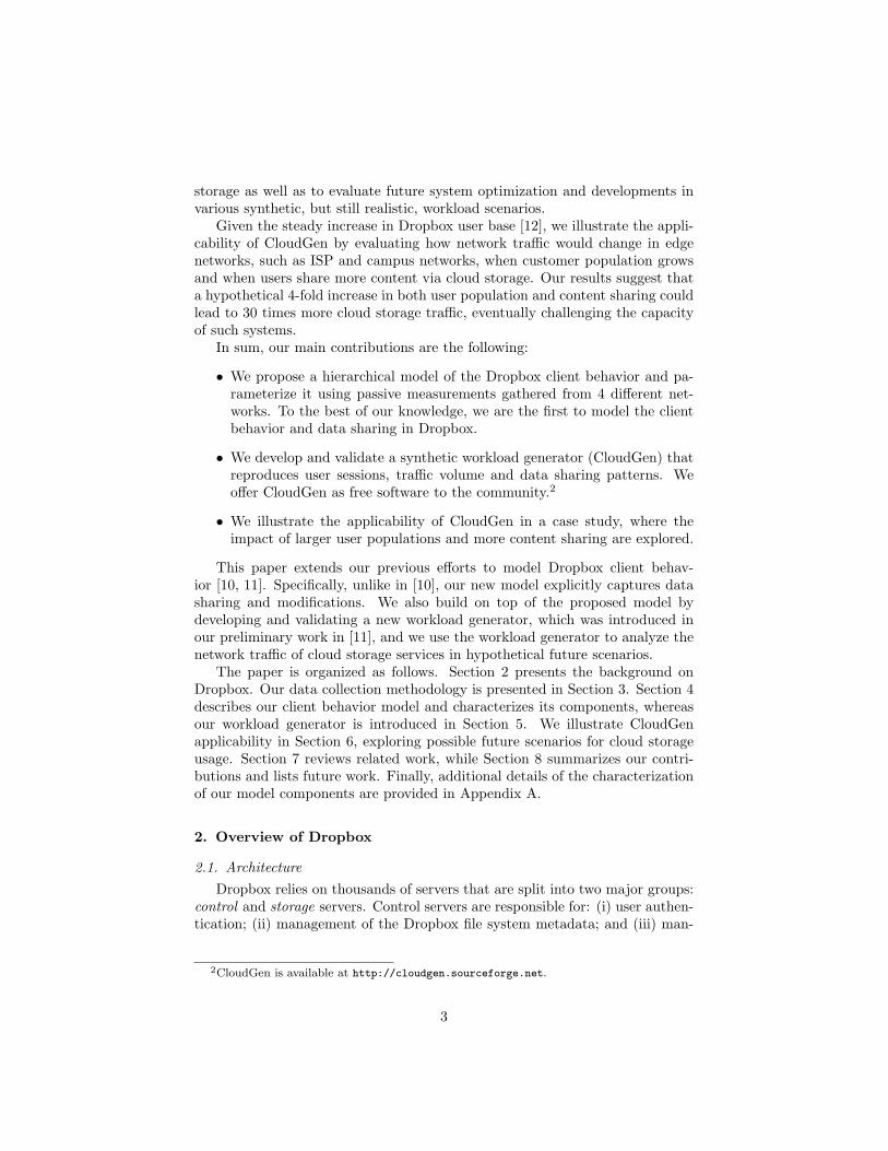
Figure 7 shows CCDFs with respective best fits for each inter-session rangein Campus-1 and PoP-1. We observe similar behavior for CCDFs of Campus-2and PoP-2. Log-normal is the best choice for all datasets in the three ranges.However, note how long inter-sessions present peculiar curves, pointing again toa complex process that is hard to be described with a simple model. Even if fitsare not tight for this range, it has little impact on generated workloads, thanksto the low frequency (5%) long inter-sessions occur in practice.

4.3.2. Namespace Layer

Namespaces per Device:

Figure 8a shows the CCDF of the number of namespaces per device. Resultsare in-line with findings in [1]. The number of devices with a single namespace issmall: around 10–22% in campus networks, and 25–35% in residential networks.Devices in campuses as well as those of users enjoying fast Internet connectiv-

6Note that we ignore inter-sessions longer than 10 days to reduce effects of seasonality.Those are less than 3% of the inter-sessions in the original data.

14


Pro

b(T

ime

>x)

5m 16m 1h 4h 12h0.00

10.

010.

11

Campus−1PoP−1Fitted Log−normal

(a) Short


Pro

b(T

ime

>x)

12h 17h 24h 33h0.00

10.

010.

11


(b) Medium


Pro

b(T

ime

>x)

33h 3d 6d 10d0.00

10.

010.

11


(c) Long

Figure 7: Inter-session times per range and best-fitted Log-normal distributions.

Namespaces per Device x

Pro

b(N

ames

pace

s>

x)

1 2 4 8 16 32 640.00

10.

010.

11


(a) All

Namespaces per Device x

Pro

b(N

ames

pace

s>

x)

1 2 4 8 160.00

10.

010.

11


(b) Per Week

Namespaces per Device xP

rob(

Nam

espa

ces

>x)

1 2 4 8 160.00

10.

010.

11

Campus−1Campus−2Fitted Neg. Binomial

(c) Best Fit – Campuses

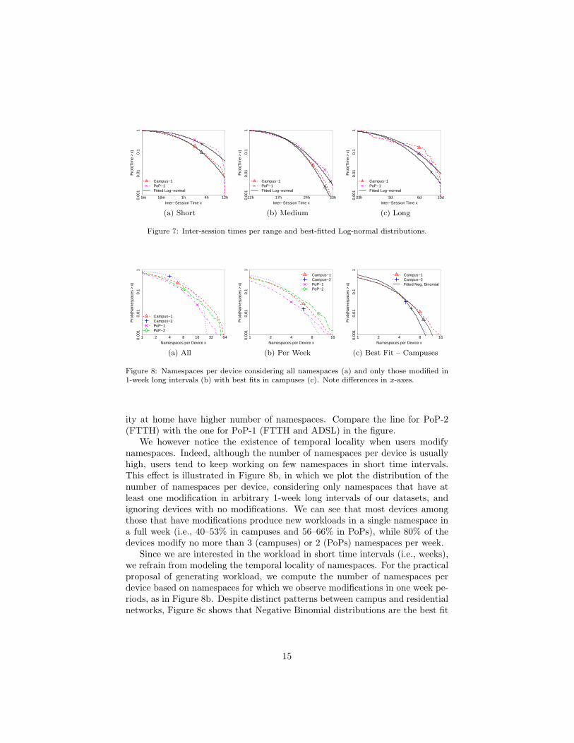
Figure 8: Namespaces per device considering all namespaces (a) and only those modified in1-week long intervals (b) with best fits in campuses (c). Note differences in x-axes.

ity at home have higher number of namespaces. Compare the line for PoP-2(FTTH) with the one for PoP-1 (FTTH and ADSL) in the figure.

We however notice the existence of temporal locality when users modifynamespaces. Indeed, although the number of namespaces per device is usuallyhigh, users tend to keep working on few namespaces in short time intervals.This effect is illustrated in Figure 8b, in which we plot the distribution of thenumber of namespaces per device, considering only namespaces that have atleast one modification in arbitrary 1-week long intervals of our datasets, andignoring devices with no modifications. We can see that most devices amongthose that have modifications produce new workloads in a single namespace ina full week (i.e., 40–53% in campuses and 56–66% in PoPs), while 80% of thedevices modify no more than 3 (campuses) or 2 (PoPs) namespaces per week.

Since we are interested in the workload in short time intervals (i.e., weeks),we refrain from modeling the temporal locality of namespaces. For the practicalproposal of generating workload, we compute the number of namespaces perdevice based on namespaces for which we observe modifications in one week pe-riods, as in Figure 8b. Despite distinct patterns between campus and residentialnetworks, Figure 8c shows that Negative Binomial distributions are the best fit

15

Number of Modifications x

Pro

b(M

odifi

catio

ns>

x)

1 10 100 10000.00

10.

010.

11


(a) All


Pro

b(M

odifi

catio

ns>

x)

1 10 100 10000.00

10.

010.

11

Campus−1Campus−2Fitted Pareto Type II



Pro

b(M

odifi

catio

ns>

x)

1 10 100 10000.00

10.

010.

11

PoP−1PoP−2Fitted Pareto Type II


Figure 9: Number of modifications. Pareto Type II distributions are the best candidate.

in campus datasets. PoP datasets are omitted for the sake of brevity, but theyprovide the same conclusion.

Namespace Selection:

We derive the methodology to select which namespaces upload content dur-ing a session. We find that the vast majority of sessions (85–93%) have nouploads at all. Clients connect to Dropbox servers, check for possible updates,but do not modify any files locally, i.e., they do not upload content. The re-maining sessions typically have modifications in a single namespace, with lessthan 2% of the sessions experiencing changes in multiple namespaces. This isexpected, since the temporal locality implies that each namespace is changed inrestrict periods of time.

Thus, for simplicity, we determine whether a session will see modificationsby computing the probability of modifications in any namespaces (e.g., 15% inCampus-1 and 7% in PoP-1). Then, we select a random namespace for eachsession that has modifications.

Number of Modifications:

We characterize the 7–15% of sessions that have at least one modification innamespaces. Figure 9 shows CCDFs of the number of modifications per session.

In general, users make few modifications in namespaces per session. Fig-ure 9a shows that, among sessions that have at least one modification, around26% have a single modification, whereas 75% of them have no more than 10modifications. However, we also observe a non-negligible number of sessionswith lots of modifications. Focusing on the tail of the distributions in Fig-ure 9a, notice that around 2% of the sessions have more than 100 modifications.Such heavy tailed distributions are well characterized by Pareto models. Indeed,we can see in Figures 9b and 9c that Pareto Type II distributions fit our datasatisfactorily, despite differences in parameters per dataset.

Inter-Modification Time:

Figure 10 shows CCDFs for inter-modification times, which are computedconsidering sessions with at least two modifications.

16

Inter−Modification Time x

Pro

b(T

ime

>x)

1s 10s 2m 1h 1d0.00

10.

010.

11


(a) All


Pro

b(T

ime

>x)

1s 10s 2m 1h 1d0.00

10.

010.

11

Campus−1Campus−2Fitted Log−Normal



Pro

b(T

ime

>x)

1s 10s 2m 1h 1d0.00

10.

010.

11

PoP−1PoP−2Fitted Log−Normal


Figure 10: Inter-modification time. Log-normal distributions are the best candidate.

Figure 10a shows that short time intervals are frequent between modifica-tions. For instance, at least 60% of the inter-modification times are shorter than1 minute in all sites. This indicates that namespaces tend to present bursts ofmodifications. Indeed, sessions with large numbers of modifications are char-acterized by such bursts. However, we also observe inter-modification times ofhours, which seems to represent the interval between bursts in long-lived ses-sions. The combination of inter- and intra-burst intervals result in distributionsthat are strongly skewed towards small values. As we can see in Figures 10band 10c, which depict CCDFs together with the best fits, Log-normal distribu-tions describe our data best.

Devices per Namespace:

The last component of the namespace layer characterizes how many deviceshave access to each namespace. Our data provide the means to estimate thenumber of devices per namespace for the user population in the networks wemonitor. Namespaces may have higher number of devices thanks to devicesconnected outside the studied networks. Thus, our characterization provides alower-bound for the actual number of devices per namespace.

Figure 11a shows CCDFs of the number of devices per namespace computedfor four networks. In contrast to the number of namespaces per device, devicesper namespace does not vary greatly when observing all namespaces registeredin the devices or only those users actually modify in a limited time interval –i.e., it is not affected by the temporal locality of namespaces. Thus, results inthe figure are computed based on all namespaces observed in each dataset.

We find that the number of devices per namespace in campuses is higherthan in PoPs: 33–36% of namespaces are shared by multiple local devices incampuses, whereas that percentage is 24–26% in PoPs. Moreover, the probabil-ity of observing a namespace with a very high number of devices in campusesis slightly greater than in residential networks (see Figure 11a). This is some-how expected, since we have already shown that devices at campuses have morenamespaces than devices at home (recall Figure 8a).

To understand these differences further, we analyze the number of devices pernamespace considering which users own the devices – i.e., disregarding devices

17

Devices per Namespace x

Pro

b(D

evic

es>

x)

1 2 4 8 160.00

10.

010.

11


(a) All


Pro

b(D

evic

es>

x)

1 2 4 8 160.00

10.

010.

11

Campus−1Campus−2Fitted Neg. Binomial



Pro

b(D

evic

es>

x)

1 2 4 8 160.00

10.

010.

11

PoP−1PoP−2Fitted Neg. Binomial


Figure 11: Devices per namespace (logarithmic scales). Most namespaces are accessed by asingle device in the network. Negative Binomial distributions best fit our data.

of the same user. We observe about 17% of namespaces are shared by multiplelocal users in campuses, whereas that percentage is 7–8% in PoPs. Thus, thepercentage of namespaces registered in devices of different users is much lowerin residential networks. These results reinforce that content sharing is moreimportant in the academic scenario, where a more consistent community ofusers is aggregated. Our residential datasets, instead, capture a scenario inwhich multiple devices of few users in a household are synchronized.

Despite differences in parameters, we find that Negative Binomial distribu-tions are the best fit for the number of devices per namespace in all sites, as weshow in Figure 11b and Figure 11c.

4.3.3. Data Transmission Layer

Finally, we study the volume of upload workloads. We characterize the vari-able using only the subset of notifications for which we have very high confidenceabout the upload volume – i.e., those notifications that occur while a single de-vice is performing uploads to a single namespace (see Figure 2a in Section 3).We expect to select a random subset of notifications, thus providing a goodestimation for the size of each workload.

Figure 12a shows CCDFs of upload sizes. Interestingly, uploads are largerin PoPs than in campuses. We conjecture that this happens because users athome often rely on cloud storage for backups and for uploading multimedia files,while a high number of small uploads is seen in campus due to interactive work.

The figure clearly shows knees in the distributions at around 10 MB forall datasets. Uploads with volume under 10 MB are the majority, e.g., 97%and 89% in Campus-1 and PoP-1, respectively. This can be explained by twofactors. First, the Dropbox client aggregates multiple small files in batches,committing transactions at arbitrary batch sizes to start content propagationwhile processing other files [1]. This strategy may bias workload sizes towardsparticular thresholds (e.g., 10 MB). Second, it has already been shown that filesizes in general are not modeled well by a single distribution model, with thebody and the tail of the empirical distribution following distinct processes [22].

18

Upload Volume x

Pro

b(V

olum

e>

x)

10B 1kB 100kB 10MB 1GB0.00

10.

010.

11


(a) All

Upload Volume x

Pro

b(V

olum

e>

x)

10B 1kB 100kB 10MB0.00

10.

010.

11


(b) Best Fit ≤ 10 MB

Upload Volume x

Pro

b(V

olum

e>

x)

10MB 30MB 100MB 300MB 1GB0.00

10.

010.

11

Campus−1PoP−1Fitted Pareto Type I

(c) Best Fit > 10 MB

Figure 12: Upload volumes. Data are best-fitted by different models at the body (Log-normal)and at the tail (Pareto Type I). Uploads at PoPs are larger than in campuses.

This suggests to break the measured data into two ranges, determining thebest fit for each range independently. Figure 12b shows the empirical distribu-tions and best fits for the measured volumes up to 10 MB, whereas Figure 12cshows curves for the volumes greater than 10 MB. Only Campus-1 and PoP-1are shown to improve visualization. In all datasets, Log-normal distributionsare the ones that better describe our data up to 10 MB (see Figure 12b). Onthe other hand, uploads with volume greater than 10 MB are best fitted by thePareto Type I distribution (see Figure 12c). Interestingly, these results are inagreement with the generative model for file sizes proposed in [22].

5. CloudGen– Cloud Storage Traffic Generator

5.1. Overview

We implement CloudGen based on our hierarchical model for the Drop-box client. CloudGen receives as input parameters for the set of distributionscharacterizing the model, as well as execution parameters, such as the syntheticworkload duration and the target number of devices (d). The latter can be freelyset to determine the population size to be evaluated. As outcome, CloudGenproduces a synthetic trace indicating when each device is active and inactive,the series of modifications in namespaces, and the data volume of modifications.Therefore, we envisage the use of CloudGen in a variety of scenarios, e.g., toevaluate the traffic users in a network produce, or to estimate the workloadservers in a cloud storage data-center face in different deployments.

CloudGen starts by setting up the content propagation network, i.e., thestructure that represents how namespaces are shared among devices (see Fig-ure 4). This process follows two steps. First, CloudGen derives the numberof distinct namespaces (n) from the number of devices (d), using the meannumber of namespaces per device (nd) and the mean number of devices pernamespace (dn), both coming from distributions characterized in Section 4.3.2.The expected number of distinct namespaces is given by n = d× nd/dn. As anexample, our data provide an average ratio of distinct namespaces per device(i.e., nd/dn) of 1.36 and 1.45 for Campus-1 and PoP-1, respectively.

19

Second, CloudGen associates devices to namespaces. For that, CloudGenincludes a method to generate random networks based on [23]: (i) CloudGen firstpicks one namespace for each device to make sure all devices have at least onenamespace; then (ii) it complements the number of devices of each namespace(sampled from the distribution of devices per namespace), by selecting randomdevices with the probability proportional to the number of namespaces in thedevices (sampled from the distribution of namespaces per device).

CloudGen then generates workloads following a classic discrete-event simu-lation approach. First, it creates a sequence of events to mark session logins andlogouts of each device. The time of each event is determined by sampling thesessions duration and the inter-session time distributions, until the next loginof all devices falls outside the synthetic trace duration.

To compute inter-session times, CloudGen samples from the inter-sessionranges (i.e., short, medium or long) based on their probabilities throughoutthe day. However, CloudGen separates devices into two groups (frequent andoccasional), and enforces only medium inter-sessions (frequent devices) or longinter-sessions (occasional devices) in night periods. As such, CloudGen mimicsthe behavior shown in Figure 6, which results in a sharp decrease in the numberof new sessions at night, and multiple-day breaks for occasional devices. Notethat while CloudGen captures intraday variations, thanks to the procedure toselect inter-session times, other seasonal patterns (e.g., weekly or yearly) areintentionally left out for the sake of simplicity.

For each session, CloudGen decides whether new events are required by fol-lowing our namespace selection strategy: First, it evaluates the probability thatany namespaces in the session are modified. When modifications should occur,CloudGen randomly selects a namespace to execute modifications. CloudGenthen determines how many modifications to place in the session. It does so byfollowing a method found on [24] to match the distribution of sessions durationwith the distribution of the number of modifications per session. Basically, thelonger sessions are, the higher are the chances they experience lots of modifica-tions. Then, the series of modification events is scheduled using the distributionof inter-modification times in a best-effort fashion: Samples of inter-modificationtimes determine the time of the next modification in the session; if the sessionduration is reached before scheduling all modifications, the remaining modifica-tions are scheduled starting from the session begin again.

CloudGen assigns the upload volume to each modification and, eventually,schedules download events using the content propagation network and the infor-mation about login and logout times of peer devices. Modifications that happenin a shared namespaces are then propagated to all peer devices. CloudGen isavailable as free software at http://cloudgen.sourceforge.net.

5.2. Validation

Methodology:

We validate CloudGen by comparing synthetic and actual traces inCampus-1 and PoP-1 datasets. We first determine the input number of devices.

20

http://cloudgen.sourceforge.net

To remove possible effects of the registration and removal of devices to/fromDropbox, we pick several weeks of data in each dataset and count the num-ber of active devices per week. Then, we execute CloudGen entering the meannumber of active devices per week in each dataset, together with the respectivedistribution parameters characterized in the previous section.

We set CloudGen to generate synthetic traces of two weeks, to make sure allranges of inter-session times are used in the simulation. Moreover, we discardthe initial week to remove simulation warm-up effects, as well as weekends sinceour model does not include such seasonality. We repeat the procedure sixteentimes for each dataset, to obtain different samples of synthetic traces.

We then contrast synthetic traces to Campus-1 and PoP-1 datasets. Wefocus on two types of metrics: (i) Direct metrics to validate that synthetictraces follow the distributions that define our model – e.g., we compute syntheticinter-session times to analyze the impact of simplifications we made to buildCloudGen; (ii) Indirect metrics that are not explicitly encoded in our model –e.g., we use the aggregated workload devices produce in pre-determined periods(e.g., per day) to check whether synthetic traces approximate well the workloadusers create to Dropbox.

Direct Metrics:

We recompute all components of our model characterized in Section 4.3, nowusing synthetic traces, to validate CloudGen implementation. For the sake ofbrevity, we show results only for Campus-1 in this first test, since PoP-1 leadsto the same conclusions. We also omit plots for sessions duration, number ofmodifications per session, upload volume and devices per namespace, since thesevariables are used directly by CloudGen, without any specific design decision tosimplify implementation.

Figure 13 summarizes metrics for which CloudGen implementation includessimplifications. We depict in each plot the empirical distribution found in actualtraces, along with the distribution extracted from the synthetic traces.

Inter-sessions times are depicted in Figures 13a. We can see that syntheticand actual distributions are tightly close to each other. Synthetic traces presentthe three-range pattern seen in actual data, with correct proportions among theranges. Thus, we can conclude that our strategy to split devices as frequent andoccasional, as well as to select inter-session ranges, works well in practice.

Figure 13b depicts inter-modification times. Since inter-modification timesare used only to distribute modifications in the sessions, and we adopt heuris-tics to match the number of modifications and the sessions duration, inter-modification times are prone to errors due to simplifications in our method. In-deed, synthetic traces present slightly more short inter-modification times thanthe actual ones. Still, the artifact affects less than 10% of the measurements,noticeable in the tail of distributions.

Finally, Figure 13c presents the number of namespaces per device, which isused indirectly as a weight when sampling devices for the content propagationnetwork. We can see that synthetic and actual traces slightly diverge in the tailof the distributions. This difference is, however, compatible with the distribution

21


Pro

b(T

ime

>x)

5m 20m 1h 4h 12h 33h 4d 10d0.00

10.

010.

11

ActualSynthetic

(a) Inter-Session Time


Pro

b(T

ime

>x)

1s 10s 2m 1h 1d0.00

10.

010.

11

ActualSynthetic

(b) Inter-Modification Time

Number of Namespaces per Device x

Pro

b(N

ames

pace

s>

x)

1 2 4 8 160.00

10.

010.

11

ActualSynthetic

(c) Namespaces per Device

Figure 13: Comparison of model components in actual and synthetic traces in Campus-1.

characterized for the variable. In fact, our method to create content propagationnetworks approximates well both distributions that characterize the Dropboxnetwork, even when small networks are created (e.g., hundreds of devices).

Overall, we conclude that our implementation is satisfactory and producessynthetic traces similar to datasets used as input to our model.

Indirect Metrics:

Next we validate CloudGen focusing on three indirect metrics: the numberof sessions, the number of modifications in namespaces and the total uploadvolume. We compute the metrics after aggregating the activity of all devicesper day. Such metrics summarize the overall workload the network and serversneed to handle in a time interval, given a fixed population of devices. Our goalis to understand whether CloudGen realistically reproduces the metrics when itis fed with the number of devices seen in actual traces.

Figure 14 presents CDFs for the indirect metrics. Top plots are relative toCampus-1, while bottom plots depict results for PoP-1.

Figure 14a and 14d show that the number of sessions per day in synthetictraces is relatively close to actual values. Focusing on Figure 14d, note how thesynthetic distribution captures the overall trend in actual data for PoP-1. Meanvalues for synthetic and actual traces are 4,542 and 4,551 in PoP-1, respectively.The number of sessions per day is slightly off actual values in Campus-1: meanof 5,649 for the synthetic trace and 5,219 for the actual one (i.e., syntheticoverestimates by 8%), and we see more variability in actual traces. This happensbecause, for the sake of simplicity, CloudGen generates similar workloads forall weekdays, while campus routine clearly varies during the week – e.g., fewerdevices are typically seen active on Wednesdays and Fridays in Campus-1. Thus,in environments with very high mobility of users, such as in campus networks,CloudGen approximates well mean values, but smooths the number of sessionsper day.

Figures 14b and 14e show distributions for the number of modifications perday. Synthetic traces follow the overall trend in actual data again, in particularregarding mean values. The mean numbers of modifications per day are 14,174(synthetic) and 13,884 (actual) in Campus-1 (synthetic overestimates by 2%),

22

0 2 4 6 8 100.0

0.2

0.4

0.6

0.8

1.0

Number of Sessions (k) x

Pro

b(N

umbe

r≤x)

ActualSynthetic

(a) Number of Sessions

0 10 20 30 400.0

0.2

0.4

0.6

0.8

1.0

Number of Modifications (k) x

Pro

b(N

umbe

r≤x)

ActualSynthetic

(b) Number of Modifications

0 10 20 30 40 50 600.0

0.2

0.4

0.6

0.8

1.0

Upload Volume (GB) x

Pro

b(V

olum

e≤

x)

ActualSynthetic

(c) Upload Volume

0 2 4 6 80.0

0.2

0.4

0.6

0.8

1.0

Number of Sessions (k) x

Pro

b(N

umbe

r≤x)

ActualSynthetic

(d) Number of Sessions

0 2 4 6 8 100.0

0.2

0.4

0.6

0.8

1.0

Number of Modifications (k) x

Pro

b(N

umbe

r≤x)

ActualSynthetic

(e) Number of Modifications

0 5 10 15 20 25 30 350.0

0.2

0.4

0.6

0.8

1.0

Upload Volume (GB) x

Pro

b(V

olum

e≤

x)

ActualSynthetic

(f) Upload Volume

Figure 14: CDFs of indirect metrics (per day) for synthetic and actual traces in Campus-1(1st. row) and PoP-1 (2nd. row). CloudGen slightly overestimates the workload.

and 4,286 (synthetic) and 4,530 (actual) in PoP-1 (synthetic underestimatesby 5%). Although mean values are closer in Campus-1 than in PoP-1, morevariability can be noticed in Campus-1 in Figure 14b, once more, thanks to theheterogeneous users’ routine in the environment throughout the week.

Figures 14c and 14f show distributions for the total upload volume per dayin Campus-1 and PoP-1, respectively. We can see that CloudGen overestimatesthe upload volume per day. Mean volumes per day are 22 GB (synthetic) and20 GB (actual) in Campus-1 (synthetic overestimates by 10%), and 14 GB (syn-thetic) and 13 GB (actual) in PoP-1 (synthetic overestimates by 8%). Syntheticmean volumes are slightly higher than actual mean volumes, despite the visualsimilarity of the distributions in the figures, due to the tails of the syntheticvolumes – i.e., few days with very high workloads in synthetic traces. Yet,synthetic values are very close to the actual ones.

We conclude that synthetic workloads capture the main trends in actualtraces. CloudGen provides conservative estimates of the upload traffic of a pop-ulation of devices, because of the heavy tailed Pareto distributions character-ized for the number and volume of uploads. CloudGen reconstructs reasonablywell the aggregated workload in typical campus and residential networks, eventhough its design is based on a per-client workload model, which is challengefor a complex system as Dropbox. CloudGen is a valuable tool, helping admin-istrators to easily provision resources for cloud storage services.

23

6. Future Scenarios for Cloud Storage Usage

6.1. Scenarios

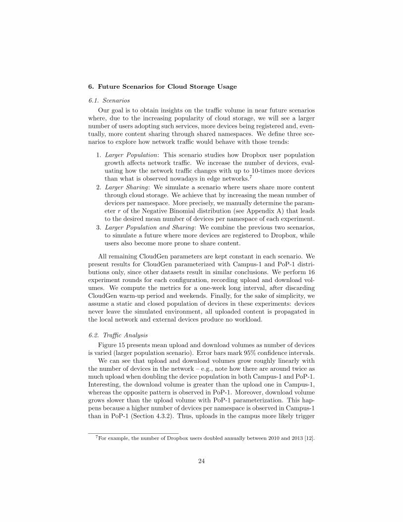
Our goal is to obtain insights on the traffic volume in near future scenarioswhere, due to the increasing popularity of cloud storage, we will see a largernumber of users adopting such services, more devices being registered and, even-tually, more content sharing through shared namespaces. We define three sce-narios to explore how network traffic would behave with those trends:

1. Larger Population: This scenario studies how Dropbox user populationgrowth affects network traffic. We increase the number of devices, eval-uating how the network traffic changes with up to 10-times more devicesthan what is observed nowadays in edge networks.7

2. Larger Sharing : We simulate a scenario where users share more contentthrough cloud storage. We achieve that by increasing the mean number ofdevices per namespace. More precisely, we manually determine the param-eter r of the Negative Binomial distribution (see Appendix A) that leadsto the desired mean number of devices per namespace of each experiment.

3. Larger Population and Sharing : We combine the previous two scenarios,to simulate a future where more devices are registered to Dropbox, whileusers also become more prone to share content.

All remaining CloudGen parameters are kept constant in each scenario. Wepresent results for CloudGen parameterized with Campus-1 and PoP-1 distri-butions only, since other datasets result in similar conclusions. We perform 16experiment rounds for each configuration, recording upload and download vol-umes. We compute the metrics for a one-week long interval, after discardingCloudGen warm-up period and weekends. Finally, for the sake of simplicity, weassume a static and closed population of devices in these experiments: devicesnever leave the simulated environment, all uploaded content is propagated inthe local network and external devices produce no workload.

6.2. Traffic Analysis

Figure 15 presents mean upload and download volumes as number of devicesis varied (larger population scenario). Error bars mark 95% confidence intervals.

We can see that upload and download volumes grow roughly linearly withthe number of devices in the network – e.g., note how there are around twice asmuch upload when doubling the device population in both Campus-1 and PoP-1.Interesting, the download volume is greater than the upload one in Campus-1,whereas the opposite pattern is observed in PoP-1. Moreover, download volumegrows slower than the upload volume with PoP-1 parameterization. This hap-pens because a higher number of devices per namespace is observed in Campus-1than in PoP-1 (Section 4.3.2). Thus, uploads in the campus more likely trigger

7For example, the number of Dropbox users doubled annually between 2010 and 2013 [12].

24

0.0

0.5

1.0

1.5

2.0

Increase (devices)

Vol

ume

(TB

)

1 2 3 4 5 6 7 8 9 10

UploadDownload

(a) Campus-1

0.0

0.5

1.0

1.5

2.0

Increase (devices)

Vol

ume

(TB

)

1 2 3 4 5 6 7 8 9 10

UploadDownload

(b) PoP-1

Figure 15: Mean upload and download volumes in larger population scenarios.

0.0

0.5

1.0

1.5

2.0

Increase (sharing)

Vol

ume

(TB

)

1 2 3 4 5 6 7 8 9 10

UploadDownload

(a) Campus-1

0.0

0.5

1.0

1.5

2.0

Increase (sharing)

Vol

ume

(TB

)

1 2 3 4 5 6 7 8 9 10

UploadDownload

(b) PoP-1

Figure 16: Mean upload and download volumes in larger sharing scenarios.

several downloads. Overall, we conclude that the network traffic of larger devicepopulations can be trivially estimated, provided that sharing behavior of usersis known and remains constant as the population increases.

Figure 16 presents mean traffic volumes for the larger sharing scenario –i.e., when we increase only the mean number of devices per namespace. Natu-rally, varying the number of devices per namespace does not affect the upload.Download volume, on the other hand, is strongly affected by the parameter. Weobserve that the download volume more than double when doubling the meannumber of devices per namespace for both Campus-1 and PoP-1. For instance,mean download volumes are 0.1, 0.3, 0.6 and 1.4 TB in Campus-1 when therespective mean number of devices per namespace is 1, 2, 4 and 8 times thevalues observed in actual traces. Similar trend can be noted for PoP-1.

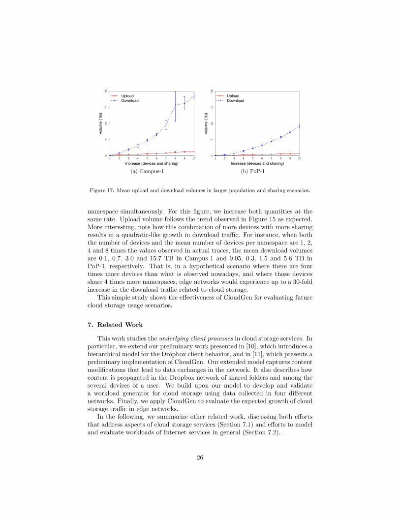
Finally, Figure 17 presents the larger population and sharing scenario, inwhich we vary both the number of devices and the mean number of devices per

25

05

1015

20

Increase (devices and sharing)

Vol

ume

(TB

)

1 2 3 4 5 6 7 8 9 10

UploadDownload

(a) Campus-1

05

1015

20

Increase (devices and sharing)

Vol

ume

(TB

)

1 2 3 4 5 6 7 8 9 10

UploadDownload

(b) PoP-1

Figure 17: Mean upload and download volumes in larger population and sharing scenarios.

namespace simultaneously. For this figure, we increase both quantities at thesame rate. Upload volume follows the trend observed in Figure 15 as expected.More interesting, note how this combination of more devices with more sharingresults in a quadratic-like growth in download traffic. For instance, when boththe number of devices and the mean number of devices per namespace are 1, 2,4 and 8 times the values observed in actual traces, the mean download volumesare 0.1, 0.7, 3.0 and 15.7 TB in Campus-1 and 0.05, 0.3, 1.5 and 5.6 TB inPoP-1, respectively. That is, in a hypothetical scenario where there are fourtimes more devices than what is observed nowadays, and where those devicesshare 4 times more namespaces, edge networks would experience up to a 30-foldincrease in the download traffic related to cloud storage.

This simple study shows the effectiveness of CloudGen for evaluating futurecloud storage usage scenarios.

7. Related Work

This work studies the underlying client processes in cloud storage services. Inparticular, we extend our preliminary work presented in [10], which introduces ahierarchical model for the Dropbox client behavior, and in [11], which presents apreliminary implementation of CloudGen. Our extended model captures contentmodifications that lead to data exchanges in the network. It also describes howcontent is propagated in the Dropbox network of shared folders and among theseveral devices of a user. We build upon our model to develop and validatea workload generator for cloud storage using data collected in four differentnetworks. Finally, we apply CloudGen to evaluate the expected growth of cloudstorage traffic in edge networks.

In the following, we summarize other related work, discussing both effortsthat address aspects of cloud storage services (Section 7.1) and efforts to modeland evaluate workloads of Internet services in general (Section 7.2).

26

7.1. Cloud Storage Services

Cloud storage services have received large attention from the research com-munity. Drago et al. [1] are the first to present an in-depth characterization oftypical usage and performance bottlenecks of Dropbox from passive measure-ments. We partly rely on their methodology to collect and process data aboutDropbox. Unlike [1], and motivated by our model for the Dropbox client behav-ior, we characterize Dropbox workload taking into account users’ sessions andcontent sharing. Moreover, we leverage the characterization to build a workloadgenerator and to evaluate possible future scenarios for Dropbox usage.

Various studies focus on benchmarking cloud storage using active experi-ments. Hu et al. [25] study the backup performance of four services. Wang etal. [26] analyze Dropbox bottlenecks, while the public APIs of three providersare compared in [9]. Authors of [3] introduce a framework to benchmark cloudstorage. Relying on an automated testing methodology, they compare designchoices and implications by benchmarking 11 services. Li et al. [8] follow asimilar methodology and compare cloud storage performance considering alsodifferent types of client terminals. None of them characterize or model thebehavior of actual cloud storage users, as we do in this work.

Some works propose alternative protocols and architectures to improve per-formance or to decrease costs of cloud storage services. In [27], a framework thatcollects semantic information from files (e.g., file type) is proposed to improveperformance of the services. Zhang et al. [5] propose a mechanism to ensure con-sistency between the local file system and remote repositories. Authors of [4]propose QuickSync, a system that optimizes synchronization by combining noveltechniques, such as network-aware chunking. Our work contributes to such ef-forts with a workload generator that can be used to evaluate new proposals inrealistic scenarios.

Finally, other works analyze cloud storage focusing on economics, security,quality of experience or privacy, and thus are orthogonal to our work. For exam-ple, authors of [28] compare pricing practices in the storage market. Mulazzaniet al. [14] uncover security issues related to the storage of content in the cloud.Quality of experience of storage services is studied in [6, 7], while the type offiles people store in the cloud are evaluated in [29].

7.2. Models and Workload Generators for Internet Services

To the best of our knowledge, we are the first to propose a model andto implement and validate a system to generate synthetic workloads for cloudstorage services, such as Dropbox.

Several models and workload generators have been proposed to create webrequest streams [24, 30–32]. Two of them model users’ behavior and its impactson network traffic and, as such, are closer to our work. SURGE [24] is a workloadgenerator that employs the concept of user equivalents to generate traffic forweb servers. SWAT [32] considers user sessions and the dependence of contentrequests within sessions. We borrow general ideas from SURGE, such as to

27

match distributions of sessions duration and number of modifications. NeitherSURGE nor SWAT, however, include mechanisms to represent the dynamics ofcontent generation and propagation as in cloud storage services. Hence, bothapproaches are insufficient to cover the particularities of such services.

Other workload generators have been proposed targeting media streamingservices. Tools like GISMO [33] and MediSyn [34] generate synthetic workloads,including client sessions and arrival patterns. Abad et al. [35] propose a gen-eral synthetic generator to create object request streams, but without includingaspects fundamental to cloud storage, such as workload volumes and sessionsduration. Closer to our work, Veloso et al. [36] and Borges et al. [37] proposehierarchical models for the behavior of users in live streaming systems. Thosemodels incorporate users’ sessions, ON/OFF times that represent active andidle periods, peering behavior and data transfers. We adopt a similar hierarchi-cal approach to model Dropbox, but focusing on a completely different type ofservice, for which both model components and parameterization differ.

Finally, our work contributes to efforts in studying cloud workloads in gen-eral. Some works focus on characterizing and modeling workloads of the cloudcomputing environment [38–40] with diverse objectives, such as to estimateCPU and memory utilization. Delimitrou et al. [41] propose a workload gen-erator that recreates I/O loads in data centers, based on inter-arrival times ofstorage access seen in application traces. Similarly, tools like CloudSim [42] aimat simulating workloads in cloud computing. CloudGen can help such effortsin reproducing workloads of cloud applications, since it models the behavior ofend-users and consequent network traffic for one of the largest cloud servicescurrently deployed (i.e., Dropbox).

8. Conclusion and Future Work

This paper investigated the workload of cloud storage services. We proposeda model to describe the Dropbox workloads, and parameterized it using datafrom four different networks. We then used our model to implement CloudGen,the first workload generator that simulates both users’ behavior and the networktraffic of cloud storage. We validated our workload generator, and illustratedits applicability by exploring the traffic volume that can be expected in futureusage scenarios. We offer CloudGen to the community as free software, as avaluable tool to simulate the behavior of cloud storage clients.

The analyses of Dropbox workloads from real data showed that our modelfor the Dropbox functioning is robust. Indeed, we found close agreement for allcomponents of the model in four distinct datasets. A summary of best-fitteddistributions for each component is provided in Appendix A.

We envision several directions for future work. Regarding extensions to ourworkload generator, we plan to model seasonality to simulate long-term dy-namics of workloads in cloud storage. We also intend to plug CloudGen inwell-known network simulators, to test the impacts of network conditions onworkloads. Moreover, we will investigate how individual user’s profile influ-ences the workload, and factor that into CloudGen, to allow the simulation of

28

populations with particular characteristics. Finally, regarding applications ofour model, we will leverage CloudGen to evaluate trade-offs (e.g., return oninvestments) of alternative architectures for cloud storage services.

9. Acknowledgments

This research is partially funded by the authors’ individual grants fromCNPq, CAPES e FAPEMIG as well as by the Brazilian National Institute ofScience and Technology for Web Research (MCT/CNPq/INCT Web Grant No.573871/2008–6).

References

[1] I. Drago, M. Mellia, M. M. Munafo, A. Sperotto, R. Sadre, A. Pras, InsideDropbox: Understanding Personal Cloud Storage Services, in: Proc. ofACM Internet Measurement Conference, 481–494, 2012.

[2] E. Bocchi, I. Drago, M. Mellia, Personal Cloud Storage: Usage, Perfor-mance and Impact of Terminals, in: Proc. of IEEE CloudNet, 2015.

[3] E. Bocchi, I. Drago, M. Mellia, Personal Cloud Storage Benchmarks andComparison, IEEE Transactions on Cloud Computing PP (99) (2015) 1–14.

[4] Y. Cui, Z. Lai, X. Wang, N. Dai, C. Miao, QuickSync: Improving Synchro-nization Efficiency for Mobile Cloud Storage Services, in: Proc. of ACMInt. Conference on Mobile Computing and Networking, 2015.

[5] Y. Zhang, C. Dragga, A. C. Arpaci-Dusseau, R. H. Arpaci-Dusseau, View-Box: Integrating Local File Systems with Cloud Storage Services, in: Proc.of the USENIX Conf. on File and Storage Technologies, 119–132, 2014.

[6] P. Amrehn, K. Vandenbroucke, T. Hossfeld, K. D. Moor, M. Hirth,R. Schatz, P. Casas, Need for Speed? On Quality of Experience for Cloud-based File Storage Services, in: Proc. of International Workshop on Per-ceptual Quality of Systems, 184–190, 2013.

[7] P. Casas, R. Schatz, Quality of Experience in Cloud Services: Survey andMeasurements, Computer Networks 68 (1) (2014) 149–165.

[8] Z. Li, C. Jin, T. Xu, C. Wilson, Y. Liu, L. Cheng, Y. Liu, Y. Dai, Z.-L.Zhang, Towards Network-Level Efficiency for Cloud Storage Services, in:Proc. of ACM Internet Measurement Conference, 115–128, 2014.

[9] R. Gracia-Tinedo, M. S. Artigas, A. Moreno-Martinez, C. Cotes, P. G.Lopez, Actively Measuring Personal Cloud Storage, in: Proc. of IEEE In-ternational Conference on Cloud Computing, 301–308, 2013.

29

[10] G. Goncalves, I. Drago, A. P. C. da Silva, A. B. Vieira, J. M. de Almeida,Modeling the Dropbox Client Behavior, in: Proc. of IEEE InternationalConference on Communications, 1332–1337, 2014.

[11] G. Goncalves, I. Drago, A. B. Vieira, A. P. C. da Silva, J. M. de Almeida,Analyzing the Impact of Dropbox Content Sharing on an Academic Net-work, in: Proc. of Brazilian Symposium on Networks and Distributed Sys-tems (in portuguese), 2015.

[12] M. Rogowsky, Dropbox Is Doing Great, But Maybe Not As Great As WeBelieved, http://onforb.es/1Kle8IE, 2013.

[13] N. Koorapati, Streaming File Synchronization, https://blogs.dropbox.com/tech/2014/07/streaming-file-synchronization/, 2014.

[14] M. Mulazzani, S. Schrittwieser, M. Leithner, M. Huber, E. Weippl, DarkClouds on the Horizon: Using Cloud Storage as Attack Vector and OnlineSlack Space, in: Proc. of the USENIX Security Symposium, 2011.

[15] A. Finamore, M. Mellia, M. Meo, M. M. Munafo, D. Rossi, Experiences ofInternet Traffic Monitoring with Tstat, IEEE Network 25 (3) (2011) 8–14.

[16] I. Bermudez, M. Mellia, M. M. Munafo, R. Keralapura, A. Nucci, DNS tothe Rescue: Discerning Content and Services in a Tangled Web, in: Proc.of ACM Internet Measurement Conference, 413–426, 2012.

[17] M. Yuksel, B. Sikdar, K. S. Vastola, B. Szymanski, Workload Generationfor NS Simulations of Wide Area Networks and the Internet, in: Proc.of the Communication Networks and Distributed Systems Modeling andSimulation Conference, 93–98, 2000.

[18] W. N. Venables, B. D. Ripley, Modern Applied Statistics with S, Springer,New York, USA, 2002.

[19] R. B. D’Agostino, M. A. Stephens, Goodness-of-Fit Techniques, MarcelDekker, New York, USA, 1986.

[20] R. K. Jain, The Art of Computer Systems Performance Analysis: Tech-niques for Experimental Design, Measurement, Simulation, and Modeling,John Wiley & Sons, New York, USA, 1991.

[21] D. Stutzbach, R. Rejaie, Understanding Churn in Peer-to-Peer Networks,in: Proc. of ACM Internet Measurement Conference, 189–202, 2006.

[22] M. Mitzenmacher, Dynamic Models for File Sizes and Double Pareto Dis-tributions, Internet Mathematics 1 (3) (2004) 305–334.

[23] K.-I. Goh, B. Kahng, D. Kim, Universal Behavior of Load Distribution inScale-Free Networks, Physical Review Letters 87 (27) (2001) 278701.

30

http://onforb.es/1Kle8IE

https://blogs.dropbox.com/tech/2014/07/streaming-file-synchronization/

https://blogs.dropbox.com/tech/2014/07/streaming-file-synchronization/

[24] P. Barford, M. Crovella, Generating Representative Web Workloads forNetwork and Server Performance Evaluation, ACM SIGMETRICS Perfor-mance Evaluation Review 26 (1) (1998) 151–160.

[25] W. Hu, T. Yang, J. N. Matthews, The Good, the Bad and the Ugly ofConsumer Cloud Storage, ACM SIGOPS Operating Systems Review 44 (3)(2010) 110–115.

[26] H. Wang, R. Shea, F. Wang, J. Liu, On the Impact of Virtualization onDropbox-Like Cloud File Storage/Synchronization Services, in: Proc. ofthe IEEE International Workshop on Quality of Service, 11:1–11:9, 2012.

[27] F. Chen, M. P. Mesnier, S. Hahn, Client-Aware Cloud Storage, in: Proc.of IEEE Symposium on Mass Storage Systems and Technologies, 2014.

[28] M. Naldi, L. Mastroeni, Cloud Storage Pricing: A Comparison of CurrentPractices, in: Proc. of ACM Int. Workshop on HotTopiCS, 27–34, 2013.

[29] S. Liu, X. Huang, H. Fu, G. Yang, Understanding Data Characteristics andAccess Patterns in a Cloud Storage System, in: Proc. of the IEEE/ACMInt. Symposium on Cluster, Cloud and Grid Computing, 327–334, 2013.

[30] D. Mosberger, T. Jin, Httperf — a Tool for Measuring Web Server Per-formance, SIGMETRICS Performance Evaluation Review 26 (3) (1998)31–37.

[31] M. Busari, C. Williamson, ProWGen: A Synthetic Workload GenerationTool for Simulation Evaluation of Web Proxy Caches, Computer Network38 (6) (2002) 779–794.

[32] D. Krishnamurthy, J. A. Rolia, S. Majumdar, A Synthetic Workload Gen-eration Technique for Stress Testing Session-Based Systems, IEEE Trans-actions on Software Engineering 32 (11) (2006) 868–882.

[33] S. Jin, A. Bestavros, GISMO: A Generator of Internet Streaming MediaObjects and Workloads, SIGMETRICS Performance Evaluation Review29 (3) (2001) 2–10.

[34] W. Tang, Y. Fu, L. Cherkasova, A. Vahdat, MediSyn: A Synthetic Stream-ing Media Service Workload Generator, in: Proc. of the Int. Workshop onNetwork and Op. Syst. Support for Digital Audio and Video, 12–21, 2003.

[35] C. L. Abad, M. Yuan, C. X. Cai, Y. Lu, N. Roberts, R. H. Campbell, Gen-erating Request Streams on Big Data using Clustered Renewal Processes,Performance Evaluation 70 (10) (2013) 704–719.

[36] E. Veloso, V. Almeida, W. M. Jr., A. Bestavros, S. Jin, A HierarchicalCharacterization of a Live Streaming Media Workload, IEEE/ACM Trans-actions on Networking 14 (1) (2006) 133–146.

31

[37] A. Borges, P. Gomes, J. Nacif, R. Mantini, J. M. de Almeida, S. Campos,Characterizing SopCast Client Behavior, Computer Communication 35 (8)(2012) 1004–1016.

[38] A. K. Mishra, J. L. Hellerstein, W. Cirne, C. R. Das, Towards Character-izing Cloud Backend Workloads: Insights from Google Compute Clusters,SIGMETRICS Performance Evaluation Review 37 (4) (2010) 34–41.

[39] Q. Zhang, J. L. Hellerstein, R. Boutaba, Characterizing Task Usage Shapesin Google’s Compute Clusters, in: Proc. of the Large Scale DistributedSystems and Middleware Workshop, 2011.

[40] I. S. Moreno, P. Garraghan, P. Townend, J. Xu, Analysis, Modeling andSimulation of Workload Patterns in a Large-Scale Utility Cloud, IEEETransactions on Cloud Computing 2 (2) (2014) 208–221.

[41] C. Delimitrou, S. Sankar, K. Vaid, C. Kozyrakis, Accurate Modeling andGeneration of Storage I/O for Datacenter Workloads, in: Proc. of the EX-ERT, 2011.

[42] R. N. Calheiros, R. Ranjan, A. Beloglazov, C. A. F. D. Rose, R. Buyya,CloudSim: A Toolkit for Modeling and Simulation of Cloud Computing En-vironments and Evaluation of Resource Provisioning Algorithms, Software-Practice & Experience 41 (1) (2011) 23–50.

Appendix A. Best-Fitted Distributions

Table A.2 lists parameters of the components of our model. The PDF of the

Log-normal distribution (parameters µ and σ) is pX(x) = 1xσ

√2π

e−(ln(x)−µ)2

2σ2 .

The PDF of the Pareto Type I distribution (parameters α and β) is

pX(x) = αβα

xα+1 . The PDF of the Pareto Type II distribution (with two pa-

rameters α and κ) is pX(x) = ακα

(x+κ)α+1 . Finally, the PDF of the Nega-

tive Binomial distribution (parameters r and p, and Gamma function Γ) is

pX(x) = Γ(x+r)Γ(r)x! p

r(1− p)x and we add 1 to generated random numbers, since

the Namespaces per Device and Devices per Namespace components are alwayslarger than zero.

32

Table A.2: Parameters of the components of our hierarchical model.

Component Model Parameters

SessionDuration (seconds)

Log-normal

Campus-1 µ = 8.222 σ = 1.395

Campus-2 µ = 8.484 σ = 1.680

PoP-1 µ = 8.209 σ = 1.464

PoP-2 µ = 8.492 σ = 1.545

Inter-SessionTime (seconds)

Range 1Log-normal

Campus-1 µ = 7.748 σ = 1.178

Campus-2 µ = 7.489 σ = 1.294

PoP-1 µ = 8.307 σ = 1.329

PoP-2 µ = 7.971 σ = 1.308


Range 2Log-normal

Campus-1 µ = 11.057 σ = 0.189

Campus-2 µ = 11.033 σ = 0.189

PoP-1 µ = 11.045 σ = 0.232

PoP-2 µ = 10.984 σ = 0.202


Range 3Log-normal

Campus-1 µ = 12.367 σ = 0.559

Campus-2 µ = 12.469 σ = 0.602

PoP-1 µ = 12.295 σ = 0.508

PoP-2 µ = 12.275 σ = 0.516

Namespacesper Device

NegativeBinomial

Campus-1 r = 0.666 p = 0.391

Campus-2 r = 1.056 p = 1.287

PoP-1 r = 0.483 p = 0.634

PoP-2 r = 0.470 p = 1.119

Number ofModifications

Pareto Type II

Campus-1 α = 1.329 κ = 5.863

Campus-2 α = 1.336 κ = 6.079

PoP-1 α = 1.534 κ = 5.601

PoP-2 α = 1.591 κ = 7.264

Inter-ModificationTime (seconds)

Log-normal

Campus-1 µ = 3.016 σ = 2.149

Campus-2 µ = 3.367 σ = 2.400

PoP-1 µ = 3.486 σ = 2.177

PoP-2 µ = 3.748 σ = 2.286

Devices perNamespace

NegativeBinomial

Campus-1 r = 0.429 p = 0.467

Campus-2 r = 0.400 p = 0.352

PoP-1 r = 0.425 p = 0.226

PoP-2 r = 0.328 p = 0.306

Upload Volume (kB)≤ 10 MB

Log-normal

Campus-1 µ = 2.288 σ = 2.582

Campus-2 µ = 1.945 σ = 3.306

PoP-1 µ = 3.417 σ = 2.721

PoP-2 µ = 2.464 σ = 2.893

Upload Volume (kB)> 10 MB

Pareto Type I

Campus-1 α = 1.291 β = 10, 000

Campus-2 α = 0.806 β = 10, 000

PoP-1 α = 1.432 β = 10, 000

PoP-2 α = 1.312 β = 10, 000

33

Workload Models and Performance Evaluation of Cloud...

Documents

Transcript of Workload Models and Performance Evaluation of Cloud...