Workload-Aware Live Storage Migration for Clouds

Workload-Aware Live Storage Migration for Clouds ∗

Jie Zheng T. S. Eugene NgRice University

Kunwadee SripanidkulchaiNECTEC, Thailand

AbstractThe emerging open cloud computing model will provide userswith great freedom to dynamically migrate virtualized computingservices to, from, and between clouds over the wide-area. Whilethis freedom leads to many potential benefits, the running servicesmust be minimally disrupted by the migration. Unfortunately, cur-rent solutions for wide-area migration incur too much disruptionas they will significantly slow down storage I/O operations duringmigration. The resulting increase in service latency could be verycostly to a business. This paper presents a novel storage migra-tion scheduling algorithm that can greatly improve storage I/O per-formance during wide-area migration. Our algorithm is unique inthat it considers individual virtual machine’s storage I/O workloadsuch as temporal locality, spatial locality and popularity character-istics to compute an efficient data transfer schedule. Using a fullyimplemented system on KVM and a trace-driven framework, weshow that our algorithm provides large performance benefits acrossa wide range of popular virtual machine workloads.

Categories and Subject Descriptors D.4.0 [Operating Systems]:General

General Terms Algorithms, Design, Experimentation, Perfor-mance

Keywords Live Storage Migration, Virtual Machine, Workload-aware, Scheduling, Cloud Computing

1. IntroductionCloud computing has recently attracted significant attention fromboth industry and academia for its ability to deliver IT servicesat a lower barrier to entry in terms of cost, risk, and expertise,with higher flexibility and better scaling on-demand. While manycloud users’ early successes have been realized using a single cloudprovider [4, 8], using multiple clouds to deliver services and having

∗ This research was sponsored by NSF CAREER Award CNS-0448546,NeTS FIND CNS-0721990, NeTS CNS-1018807, by an IBM FacultyAward, an Alfred P. Sloan Research Fellowship, and by Microsoft Corp.Jie Zheng is additionally supported by an IBM Scholarship. Views and con-clusions contained in this document are those of the authors and should notbe interpreted as representing the official policies, either expressed or im-plied, of NSF, IBM Corp., Microsoft Corp., the Alfred P. Sloan Foundation,or the U.S. government.

Permission to make digital or hard copies of all or part of this work for personal orclassroom use is granted without fee provided that copies are not made or distributedfor profit or commercial advantage and that copies bear this notice and the full citationon the first page. To copy otherwise, to republish, to post on servers orto redistributeto lists, requires prior specific permission and/or a fee.

VEE’11, March 9–11, 2011, Newport Beach, California, USA.Copyright c© 2011 ACM 978-1-4503-0501-3/11/03. . . $10.00

the flexibility to move freely among different providers is an emerg-ing requirement [1]. The Open Cloud Manifesto is an example ofhow users and vendors are coming together to support and estab-lish principles in opening up choices in cloud computing [16]. Akey barrier to cloud adoption identified in the manifesto is data andapplication portability. Users who implement their applications us-ing one cloud provider ought to have the capability and flexibility tomigrate their applications back in-house or to other cloud providersin order to have control over business continuity and avoid fate-sharing with specific providers.

In addition to avoiding single-provider lock-in, there are otheravailability and economic reasons driving the requirement for mi-gration across clouds. To maintain high performance and availabil-ity, virtual machines (VMs) could be migrated from one cloud toanother cloud to leverage better resource availability, to avoid hard-ware or network maintenance down-times, or to avoid power limi-tations in the source cloud. Furthermore, cloud users may want tomove work to clouds that provide lower-cost. The current practicefor migration causes significant transitional down time. In orderfor users to realize the benefits of migration between clouds, weneed both open interfaces and mechanisms to enable such migra-tion while the services are running with as minimal service disrup-tion as possible. While providers are working towards open inter-faces, in this paper we look at the enabling mechanisms withoutwhich migrations would remain a costly effort.

Live migration provides the capability to move VMs fromone physical location to another while still running without anyperceived degradation. Many hypervisors support live migrationwithin the LAN [6, 10, 13, 17, 20, 25]. However, migrating acrossthe wide area presents more challenges specifically because of thelarge amount of data that needs to be migrated over limited net-work bandwidth. In order to enable live migration over the widearea, three capabilities are needed: (i) the running state of the VMmust be migrated (i.e., memory migration), (ii) the storage or vir-tual disks used by the VM must be migrated, and (iii) existingclient connections must be migrated while new client connectionsare directed to the new location. Memory migration and networkconnection migration for the wide area have been demonstratedto work well [5, 24]. However, storage migration inherently facessignificant performance challenges because of its much larger sizecompared to memory.

In this paper, we improve the efficiency of migrating storageacross the wide area. Our approach differs from the existing work instorage migration that treats storage as one large chunk that needsto be transferred from beginning to end. We introducestorage mi-gration schedulingto transfer storage blocks according to a deliber-ately computed order. We develop a workload-aware storage migra-tion scheduling algorithm that takes advantage of temporal locality,spatial locality, and access popularity – patterns commonly foundin a wide range of I/O workloads – at the properly chosen gran-ularity to optimize the data transfer. We show that our schedulingalgorithm can be leveraged by previous work in storage migration

Im age file transfer

(beg inn ing to end)

M em ory

m igra tion

O n-dem and fe tch ing

P re-copy m odel w ithout schedu ling

P re+post-copy m odel w ithout schedu ling

P ost-copy m odel w ithout schedu ling

M em ory

m igra tion





M em ory

m igra tionO n-dem and

Transfe r

d irty b locks

ID sequence

N on-w ritten

chunks

M em ory

m igra tion

O n-dem and fe tch ing

P re-copy m odel w ith schedu ling

P re+post-copy m odel w ith schedu ling

P ost-copy m odel w ith scheduling

M em ory

m igra tion

Sorted

read chunks

h igh→low

M em ory

m igra tionO n-dem and

Sorted read

d irty b locks

h igh→low

H istory

(log

write op)

H istory

(log

read op)

H istory

(log

read &

write op)

Sorted

w ritten chunks

low h igh

N on-read chunks

N on-w ritten

chunks

S orted

written chunks

low →high

T ransfer

d irty b locks

ID sequence

S orted

d irty b locks

low high

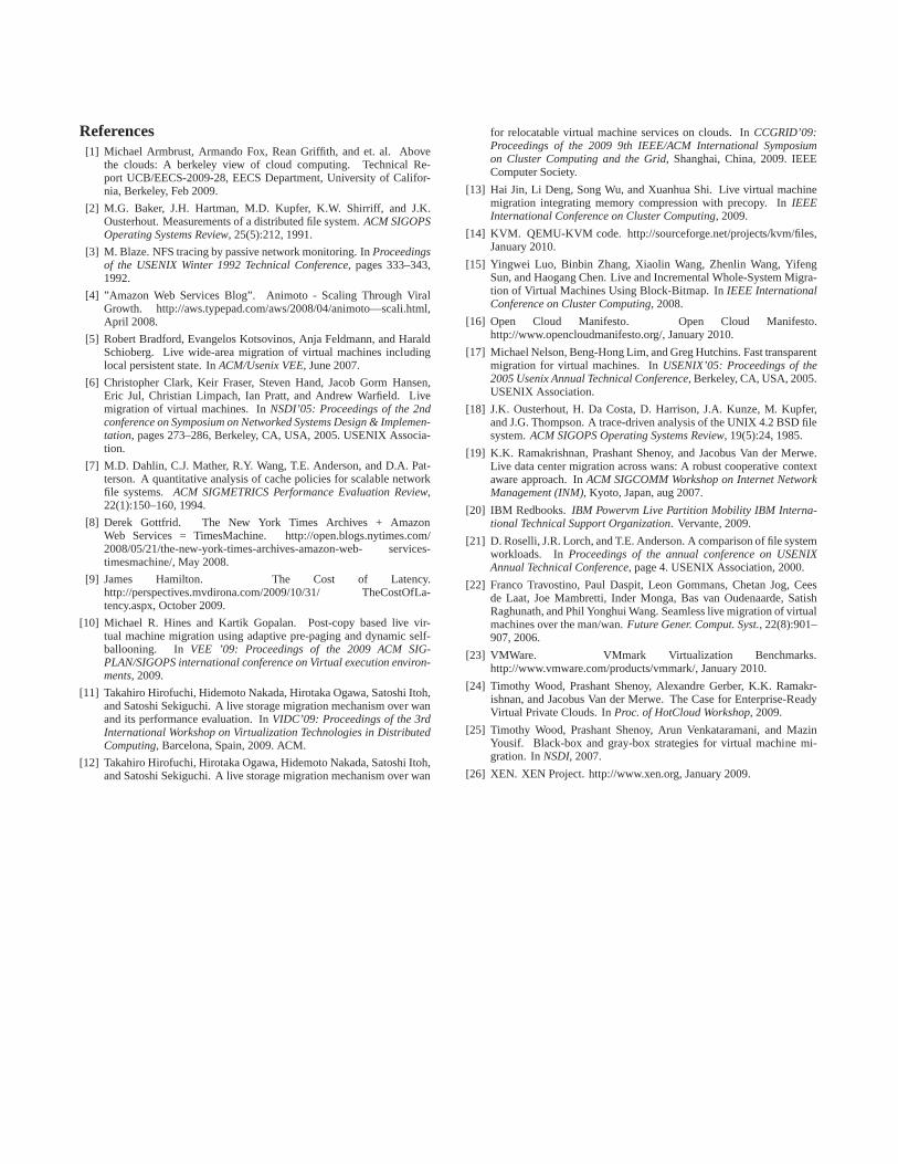
Figure 1. Models of live storage migration.

to greatly improve storage I/O performance during migration acrossa wide variety of VM workloads.

In the next section, we provide an overview of the existing stor-age migration technologies and the challenges that they face. Sec-tion 3 quantifies the locality and popularity characteristics we foundin VM storage workload traces. Motivated by these characteristics,we present in Section 4 a novel storage migration scheduling al-gorithm that leverages these characteristics to make storage migra-tion much more efficient. We present the implementation of ourscheduling algorithm on KVM in Section 5 and evaluate its perfor-mance in Section 6. In Section 7, we further present trace-basedsimulation results for the scheduling algorithm under two addi-tional migration models not adopted by KVM. Finally, we sum-marize our findings in Section 8.

2. BackgroundA VM consists of virtual hardware devices such as CPU, memoryand disk. Live migration of a VM within a data center is quite com-mon. It involves the transfer of the memory and CPU state of theVM from one hypervisor to another. However, live migration acrossthe wide area requires not only transferring the memory and CPUstate, but also virtual disk storage and network connections associ-ated with a VM. While wide-area memory and network connectionmigration have matured [5, 19, 22, 24], wide-area storage migrationstill faces significant performance challenges. The VM’s disk is im-plemented as a (set of) file(s) stored on the physical disk. Becausesharing storage across the wide area has unacceptable performance,storage must be migrated to the destination cloud. And becauseof the larger size storage has compared to memory and the limi-tations in wide-area network bandwidth, storage migration couldnegatively impact VM performance if not performed efficiently.

2.1 Storage Migration Models

Previous work in storage migration can be classified into threemigration models: pre-copy, post-copy and pre+post-copy. In thepre-copy model, storage migration is performedprior to memorymigration whereas in the post-copy model, the storage migration isperformedafter memory migration. The pre+post-copy model is ahybrid of the first two models.

Figure 1 depicts the three models on the left-hand side. In thepre-copy model as implemented by KVM [14] (a slightly differentvariant is also found in [5]), the entire virtual disk file is copiedfrom beginning to end prior to memory migration. During the vir-tual disk copy, all write operations to the disk are logged. The dirtyblocks are retransmitted, and new dirty blocks generated during thistime are again logged and retransmitted. This dirty block retrans-mission process repeats until the number of dirty blocks falls belowa threshold, then memory migration begins. During memory mi-gration, dirty blocks are again logged and retransmitted iteratively.

The strength of the pre-copy model is that VM disk read opera-tions at the destination have good performance because blocks arecopied over prior to when the VM starts running at the destination.However, the pre-copy model has weaknesses. First, pre-copyingmay introduce extra traffic. If we had an oracle that told us whendisk blocks are updated, we would send only the latest copy of diskblocks. In this case, the total number of bytes transferred over thenetwork would be the minimum possible which is the total size ofthe virtual disk. Without an oracle, some transmitted blocks willbecome dirty and require retransmissions, resulting inextra traf-fic beyond the size of the virtual disk. Second, if the I/O workloadon the VM is write-intensive, write-throttling is employed to slowdown I/O operations so that iterative dirty block retransmission canconverge. While throttling is useful, it can degrade application I/Operformance.

In the post-copy model [11, 12], storage migration is executedafter memory migration completes and the VM is running at thedestination. Two mechanisms are used to copy disk blocks over:background copying and remote read. In background copying, thesimplest strategy proposed by Hirofuchi et al. [12] is to copy blockssequentially from the beginning of a virtual disk to the end. Theyalso proposed an advanced background copy strategy which willbe discussed later in Section 2.3. During this time if the VM is-sues an I/O request, it is handled immediately. If the VM issues awrite operation, the blocks are directly updated at the destinationstorage. If the VM issues a read operation and the blocks have yetto arrive at the destination, then on-demand fetching is employedto request those blocks from the source. We call such operationsremote reads. With the combination of background copying and re-mote reads, each block is transferred at most once ensuring that thetotal amount of data transferred for storage migration is minimized.However, remote reads incur extra wide-area delays, resulting inI/O performance degradation.

In the hybrid pre+post-copy model [15], the virtual disk iscopied to the destination prior to memory migration. During diskcopy and memory migration, a bit-map of dirty disk blocks is main-tained. After memory migration completes, the bit-map is sent tothe destination where a background copying and remote read modelis employed for the dirty blocks. While this model still incurs extratraffic and remote read delays, the amount of extra traffic is smallercompared to the pre-copy model and the number of remote readsis smaller compared to the post-copy model. Table 1 summarizesthese three models.

2.2 Performance Degradation from Migration

While migration is a powerful capability, any performance degra-dation caused by wide area migration could be damaging to usersthat are sensitive to latency. Anecdotally, every 100 ms of latencycosts Amazon 1% in sales and an extra 500 ms page generation timedropped 20% of Google’s traffic [9]. In our analysis (details in Sec-tion 7) of a 10 GB MySQL database server that has 160 clients mi-grating over a 100 Mbps wide area link using the post-copy model,over 25,000 read operations experience performance degradationduring migration due to remote read. This I/O performance degra-dation can significantly impact application performance on the VM.Reducing this degradation is key to making live migration a practi-cal mechanism for moving applications across clouds.

2.3 Our Solution

Our solution is calledworkload-aware storage migration schedul-ing. Rather than copying the storage from beginning to end, wedeliberately compute a schedule to transfer storage at the appropri-ate granularity which we callchunkand in the appropriate orderto minimize performance degradation. Our schedule is computedto take advantage of the particular I/O locality characteristics of

Model Pre-copy [5, 14] Pre+post-copy [15] Post-copy [11, 12]Application Write Operation Degradation Yes No NoPerformance Read Operation Degradation No Medium Heavy

Impact Degradation Time Long Medium LongI/O Operations Throttled Yes No No

Total Migration Time >> Best > Best BestAmount of Migrated Data >> Best > Best Best

Table 1. Comparison of VM storage migration methods.

the migrated workload and can be applied to improve any of thethree storage migration models as depicted on the right-hand sideof Figure 1. To reduce the extra migration traffic and throttling un-der the pre-copy model, our scheduling algorithm groups storageblocks into chunks and sends the chunks to the destination in anoptimized order. Similarly, to reduce the number of remote readsunder the post-copy model, scheduling is used to group and or-der storage blocks sent over during background copying. In the hy-brid pre+post-copy model, scheduling is used for both the pre-copyphase and the post-copy phase to reducing extra migration trafficand remote reads.

Hirofuchi et al. [12] proposed an advanced strategy for back-ground copying in the post-copy model by recording and trans-ferring frequently accessed ext2/3 block groups first. While theirproposal is similar in spirit to our solution, there are important dif-ferences. First, their proposal is dependent on the use of an ext2/3file system in the VM. In contrast, our solution is general withoutany file system constraints, because we track I/O accesses at theraw disk block level which is beneath the file system. Second, theaccess recording and block copying in their proposal are based ona fixed granularity, i.e. an ext2/3 block group. However, our solu-tion is adaptive to workloads. We propose algorithms to leveragethe locality characteristics of workloads to decide the appropriategranularity. As our experiments show, using an incorrect granular-ity leads to a large loss of performance. Third, we show how our so-lution can be applied to all three storage migration models and ex-perimentally quantify the storage I/O performance improvements.

To our knowledge, past explorations in memory migration [6,10] leverage memory access patterns to decide which memorypages to transfer first to some extent. However, comparing to ourtechnique, there are large differences.

In a pre-copy model proposed by Clark et al. [6], only duringthe iterative dirty page copying stage, the copying of pages thathave been dirtied both in the previous iteration and the currentiteration is postponed. In a post-copy model proposed by Hines andGopalan [10], when a page that causes a page fault is copied, a setof pages surrounding the faulting page is copied together. This isdone regardless of the actual popularity of the set of surroundingpages, and continues until the next page fault occurs.

In contrast, our scheduling technique for storage migration (1)is general for the three storage migration models as discussedabove, (2) uses actual access frequencies, (3) computes fine-grainedaccess-frequency-based schedules for migration throughout thedisk image copying stage and the iterative dirty block copyingstage, (4) automatically computes the appropriate chunk size forcopying, and (5) proactively computes schedules based on a globalview of the entire disk image and the access history, rather thanreacting to each local event. Furthermore, under typical workloads,memory and storage access patterns are different, and the con-straints in the memory and storage subsystems are different. Tech-niques that work well for one may not necessarily work well for theother. Our technique is tailored specifically for storage migrationand storage access pattern.

Workload VM Configuration Server Default #Name Application ClientsFile SLES 10 32-bit dbench 45

Server (fs) 1 CPU,256MB RAM,8GB diskMail Windows 2003 32-bit Exchange 1000

Server (ms) 2 CPU,1GB RAM,24GB disk 2003Java Windows 2003 64-bit SPECjbb 8

Server (js) 2 CPU,1GB RAM,8GB disk @2005-basedWeb SLES 10 64-bit SPECweb 100

Server (ws) 2 CPU,512MB RAM,8GB disk @2005-basedDatabase SLES 10 64-bit MySQL 16

Server (ds) 2 CPU,2GB RAM,10GB disk

Table 2. VMmark workload summary.

3. Workload CharacteristicsTo investigate storage migration scheduling, we collect and study amodest set of VMware VMmark virtualization benchmark [23] I/Otraces. Our trace analysis explores several I/O characteristics at thetime-scale relevant to storage migration to understand whether thehistory of I/O accesses prior to a migration is useful for optimizingstorage migration. It is complementary to existing general studiesof other storage workloads [2, 18, 21].

3.1 Trace Collection

VMmark includes servers, listed in Table 2, that are representa-tive of the applications run by VMware users. We collect tracesfor multiple client workload intensities by varying the number ofclient threads. A trace is named according to the server type andthe number of client threads. For example, “fs-45” refers to a fileserver I/O trace with 45 client threads. Two machines with a 3GHzQuad-core AMD Phenom II 945 processor and 8GB of DRAM areused. One machine runs the server application while the other runsthe VMmark client. The server is run as a VM on a VMware ESXi4.0 hypervisor. The configuration of the server VM and the clientis as specified by VMmark. To collect the I/O trace, we run an NFSserver as a VM on the application server physical machine andmount it on the ESXi hypervisor. The application server’s virtualdisk is then placed on the NFS storage as a VMDK flat format file.tcpdump is used on the virtual network interface to log the NFSrequests that correspond to virtual disk I/O accesses. NFS-basedtracing has been used in past studies of storage workload [3, 7] andrequires no special OS instrumentation. We experimentally con-firmed that the tracing framework introduces negligible applicationperformance degradation compared to placing the virtual disk di-rectly on the hypervisor’s locally attached disk. We trace I/O oper-ations at the disk sector granularity – 512 bytes. We call each 512byte sector a block. However, this is generally not the file systemblock size. Each trace entry includes the access time, read or write,the offset in the VMDK file, and the data length. Each trace con-tains the I/O operations executed by a server over a 12 hour period.

3.2 History and Migration Periods

Let t denote the start time of a migration. Each I/O trace analysisis performed 20 times with different randomly selected migrationstart timest ∈ [3000s, 5000s], where0s represents the beginningof the trace. For simplicity, we use a fixed history period of 3000seconds beforet, and a fixed storage migration period of(2 ×image size + memory size) / bandwidth seconds. The latter

0

20

40

60

80

100

Fileserver Mailserver Javaserver Webserver DB server

Per

cent

age

of I/

O a

cces

ses

from

pre

viou

s ac

cess

es (

%)

Workload

Read blocksWritten blocksRead chunks

Written chunks

Figure 2. The temporal locality of I/O accesses as measured by thepercentage of accesses in the migration that was also previouslyaccessed in the history. The block size is 512B and the chunksize is 1MB. Temporal locality exists in all of the workloads, butis stronger at the chunk level. The Java server has very few readaccesses resulting in no measurable locality.

corresponds to a pessimistic case that during the transfer of thedisk image, all the blocks were written to by the VM and theentire image needs to be retransmitted. Other reasonable choicesfor these periods could be used, but the qualitative findings from ouranalysis are not expected to change.image size, memory size,and workload (i.e. # client threads) are as specified in Table 2, andbandwidth is 100 Mbps in the following analysis.

3.3 Temporal Locality Characteristics

Figure 2 shows that, across all workloads, blocks that are readduring the migration are often also the blocks that were read in thehistory. Take the file server as an example, 72% of the blocks thatare read in the migration were also read in the history. Among theseblocks, 96% of them are blocks whose read access frequencies were≥ 3 in the history. Thus, it is possible to predict which blocks aremore likely to be read in the near future by analyzing the recentpast history.

However, write accesses do not behave like the read accesses.Write operations tend to access new blocks that have not beenwritten before. Again, take the file server as an example. Only32% of the blocks that are written in the migration were writtenin history. Therefore, simply counting the write accesses in historywill poorly predict the write accesses in migration.

Figure 2 also shows that both read and write temporal localityimproves dramatically when 1MB chunk is used as the basic unitof counting accesses. This is explained next.

3.4 Spatial Locality Characteristics

We find strong spatial locality for write accesses. Take the fileserver as an example. For the 68% of the blocks that are freshlywritten in migration but not in history, we compute the dis-tance between each of these blocks and its closest neighborblock that was written in history. The distance is defined as(block id difference ∗ blocksize). Figure 3 plots, for the fileserver, the cumulative percentage of the fresh written blocks ver-sus the closest neighbor distance normalized by the storage size(8GB). For all the fresh written blocks, their closest neighbors canbe found within a distance of 0.0045*8GB=36.8MB. For 90% ofthe cases, the closest neighbor can be found within a short distanceof 0.0001*8GB=839KB. For comparison, we also plot the resultsfor an equal number of simulated random write accesses, whichconfirm that the spatial locality found in the real trace is significant.Taken together, in the file server trace,32%+68%∗90% = 93.2%

0

0.1

0.2

0.3

0.4

0.5

0.6

0.7

0.8

0.9

1

1e-07 1e-06 1e-05 0.0001 0.001 0.01 0.1

Per

cent

age

of th

e fr

esh

writ

ten

bloc

ks

Distance / Storage size

Actual accesses from traceSimulated random accesses

Figure 3. Spatial locality of file server writes and simulated ran-dom writes measured by normalized distance to closest block writ-ten in history. The 90th percentiles are 0.0001 and 0.0035.

of the written blocks in the migration are found within a range of839KB of the written blocks in history.

This explains why, across all workloads, the temporal locality ofwrite accesses increases dramatically in Figure 2 when we consider1MB chunk instead of 512B block as the basic unit of countingaccesses. The temporal locality of read accesses also increases. Thecaveat is that as the chunk size increases, although the percentage ofcovered accessed blocks in migration will increase, each chunk willalso cover more unaccessed blocks. Therefore, to provide usefulread and write access prediction, a balanced chunk size is necessaryand will depend on the workload (see Section 4).

3.5 Popularity Characteristics

Popular chunks in history are also likely to be popular in migration.We rank chunks by their read/write frequencies and compute therank correlation between the ranking in history and the ranking inmigration. Figure 4 shows that a positive correlation exists for allcases except for the Java server read accesses at 1MB and 4MBchunk sizes.1 As the chunk size increases, the rank correlationincreases. This increase is expected since if the chunk size is setto the size of the whole storage, the rank correlation will become1 by definition. A balanced chunk size is required to exploit thispopularity characteristic effectively (see Section 4).

4. Scheduling AlgorithmThe main idea of the algorithm is to exploit locality to computea more optimized storage migration schedule. We intercept andrecord a short history of the recent disk I/O operations of the VM,then use this history to predict the temporal locality, spatial local-ity, and popularity characteristics of the I/O workload during mi-gration. Based on these predictions, we compute a storage trans-fer schedule that reduces the amount of extra migration traffic andthrottling in the pre-copy model, the number of remote reads inthe post-copy model, and reduces both extra migration traffic andremote reads in the pre+post-copy model. The net result is that stor-age I/O performance during migration is greatly improved. The al-gorithm presented below is conceptual. In Section 5, we presentseveral implementation techniques.

4.1 History of I/O Accesses

To collect history, we record the most recentN I/O operations ina FIFO queue. We will show that the performance improvement issignificant even with a smallN in Section 6 and 7. Therefore the

1 This is because the Java server has extremely few read accesses and littleread locality

-0.8

-0.6

-0.4

-0.2

0

0.2

0.4

0.6

0.8

1

1.2


The

ran

k co

rrel

atio

n of

the

chun

k po

pula

rity

Workload

Chunk Size 1MBChunk Size 4MB


(a) Read Access

0

0.2

0.4

0.6

0.8

1


The

ran

k co

rrel

atio

n of

the

chun

k po

pula

rity

Workload



(b) Write Access

Figure 4. The rank correlation of the chunk popularity in history vs. in migration.

(c) Scheduling on the access frequency of chunks.

Extra traffic = 0 blocks

No write access in history

7 8 9 10 3 4 5 6 1 2

……

Sorted with write frequency

time

3 1 2 1 2 34 2 4 2 5 1 6 1 2 1 2

Memory

migration

Transfer

dirty

blocks

Unique Dirty Blocks = { }

Frequency

Of Block

3,4,<5,6<1,2

History

5 3 5 1 2 21 2 1 2

No write access in history

4 6 7 8 9 10 3 5 1 2Frequency

Of Block

3<5<1<2

History

……

Sorted with write frequency

time

(b) Scheduling on the access frequency of blocks.

Extra traffic = 2 blocks

3 1 2 1 2 34 2 4 2 5 1 6 1 2 1 2

Memory

migration

5 3 5 1 2 21 2 1 2

Transfer

dirty

blocks

Unique Dirty Blocks = {4, 6}

Written Block

Block Sequence in Storage Migration

Migrated Block

……

time

Write

Sequence

1 2 3 4 5 6 7 8 9 10

Blocks Written After Migration

3 1 2 1 2 34 2 4 2 5 1 6 1 2 1 2

(a) No scheduling. Extra traffic = 6 blocks

Unique Dirty Blocks = {1, 2, 3, 4, 5, 6}

Memory

migration

Transfer

dirty

blocks

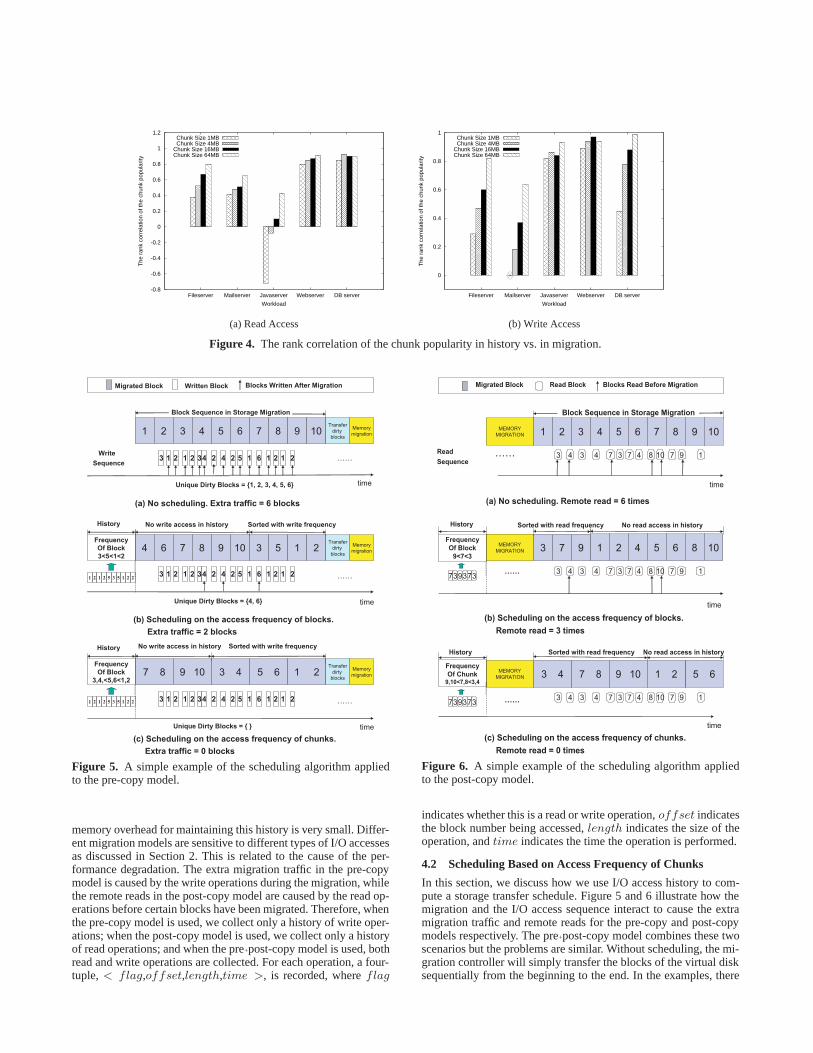
Figure 5. A simple example of the scheduling algorithm appliedto the pre-copy model.

memory overhead for maintaining this history is very small. Differ-ent migration models are sensitive to different types of I/O accessesas discussed in Section 2. This is related to the cause of the per-formance degradation. The extra migration traffic in the pre-copymodel is caused by the write operations during the migration, whilethe remote reads in the post-copy model are caused by the read op-erations before certain blocks have been migrated. Therefore, whenthe pre-copy model is used, we collect only a history of write oper-ations; when the post-copy model is used, we collect only a historyof read operations; and when the pre+post-copy model is used, bothread and write operations are collected. For each operation, a four-tuple, < flag,offset,length,time >, is recorded, whereflag

……

time

1 2 4 5 6 8 10

3

MEMORY

MIGRATION

3 4 7 73 4 8 10 7 9 14

Frequency

Of Block

9<7<3

History

739373

No read access in historySorted with read frequency

(b) Scheduling on the access frequency of blocks.

Remote read = 3 times

3 7 9

……

time

3

MEMORY

MIGRATION

3 4 7 73 4 8 10 7 9 14

Frequency

Of Chunk9,10<7,8<3,4

History

739373

No read access in historySorted with read frequency

(c) Scheduling on the access frequency of chunks.

Remote read = 0 times

5 67 8 9 103 4 1 2

Block Sequence in Storage Migration

Migrated Block

……

time

Read

Sequence

1 2 3 4 5 6 7 8 9 10

Blocks Read Before Migration

(a) No scheduling. Remote read = 6 times

Read Block

3

MEMORY

MIGRATION

3 4 7 73 4 8 10 7 9 14

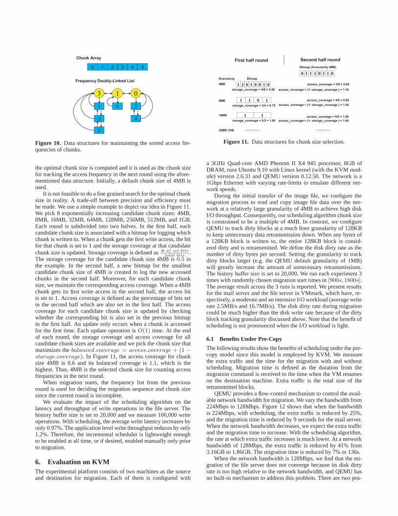
Figure 6. A simple example of the scheduling algorithm appliedto the post-copy model.

indicates whether this is a read or write operation,offset indicatesthe block number being accessed,length indicates the size of theoperation, andtime indicates the time the operation is performed.

4.2 Scheduling Based on Access Frequency of Chunks

In this section, we discuss how we use I/O access history to com-pute a storage transfer schedule. Figure 5 and 6 illustrate how themigration and the I/O access sequence interact to cause the extramigration traffic and remote reads for the pre-copy and post-copymodels respectively. The pre+post-copy model combines these twoscenarios but the problems are similar. Without scheduling, the mi-gration controller will simply transfer the blocks of the virtual disksequentially from the beginning to the end. In the examples, there

are only 10 blocks for migration and several I/O accesses denotedas either the write or read sequence. With no scheduling, under pre-copy, a total of 6 blocks are dirtied after they have been transmittedand have to be resent. Similarly, under post-copy, there are 6 remoteread operations where a block is needed before it is transferred tothe destination.

Our scheduling algorithm exploits the temporal locality andpopularity characteristics and uses the information in the historyto perform predictions. That is, the block with a higher write fre-quency in history (i.e., more likely to be written to again) should bemigrated later in the pre-copy model, and the block with a higherread frequency (i.e., more likely to be read again) should be mi-grated earlier in the post-copy model. In the illustrative example inFigures 5 and 6, when we schedule the blocks according to their ac-cess frequencies, the extra traffic and remote reads can be reducedfrom 6 to 2 and from 6 to 3 respectively.

In the example, blocks{4,6} in the pre-copy model and blocks{4,8,10} in the post-copy model are not found in the history, butthey are accessed a lot during the migration due to spatial locality.The scheduling algorithm exploits spatial locality by scheduling themigration based on chunks. Each chunk is a cluster of contiguousblocks. The chunk size in the simple example is 2 blocks. We notethat different workloads may have different effective chunk sizesand present a chunk size selection algorithm later in Section 4.3.

The access frequency of a chunk is defined as the sum of theaccess frequencies of the blocks in that chunk. The schedulingalgorithm for the pre-copy model migrates the chunks that havenot been written to in history first as those chunks are unlikely tobe written to during migration and then followed by the writtenchunks. The written chunks are further sorted by their access fre-quencies to exploit the popularity characteristics. For the post-copymodel, the read chunks are migrated in decreasing order of chunkread access frequencies, and then followed by the non-read chunks.The schedule ensures that chunks that have been read frequently inhistory are sent to the destination first as they are more likely tobe accessed. In the example, by performing chunk scheduling, theextra traffic and remote reads are further reduced to 0.

The scheduling algorithm is summarized in pseudocode as Fig-ure 7 shows. The time complexity isO(n · log(n)), the space com-plexity isO(n), wheren is the number of blocks in the disk.

Note thatα is an input value for the chunk size estimationalgorithm and will be explained later. The pre+post-copy model is aspecial case which has two migration stages. The above algorithmworks for its first stage. The second stage begins when the VMmemory migration has finished. In this second stage, the remainingdirty blocks are scheduled from high to low read frequency. Thetime complexity isO(n · log(n)), the space complexity isO(n),wheren is the number of dirty blocks.

The scheduling algorithm relies on the precondition that the ac-cess history can help predict the future accesses during migration,and our analysis has shown this to be the case for a wide range ofworkloads. However, an actual implementation might want to in-clude certain safeguards to ensure that even in the rare case that theaccess characteristics are turned upside down during the migration,any negative impact is contained. First, a test can be performed onthe history itself, to see if the first half of the history does providegood prediction for the second half. Second, during the migration,newly issued I/O operations can be tested against the expected ac-cess patterns to find out whether they are consistent. If either oneof these tests fails, a simple solution is to revert to the basic non-scheduling migration approach.

4.3 Chunk Size Selection

The chunk size used in the scheduling algorithm needs to be ju-diciously selected. It needs to be sufficiently large to cover the

DATA STRUCTURE IN ALGORITHM:-op flag: the flag of operation to indicate it is a read or a write-Qhistory : the queue of access operations collected from history-α: the fraction of simulated history.-Lb(op flag): A block access list of< blockid, time >-Lcfreq(op flag): A list of < chunkid, frequency >-Lschunk(op flag): A list of chunkid sorted by frequency-Lnchunk(op flag): A list of chunkid not accessed in history

INPUT OF ALGORITHM:Qhistory , model flag andα ∈[0, 1]OUTPUT OF ALGORITHM: migration scheduleSmigration

Smigration = { };IF ((model flag == PRE COPY )‖(model flag == PRE + POST COPY ))

Smigration=GetSortedMigrationSequence(WRITE);ELSE (model flag == POST COPY )

Smigration=GetSortedMigrationSequence(READ);RETURNSmigration;

FUNCTION GetSortedMigrationSequence(op flag)Lb(op flag) = Convert∀OP ∈ Qhistory

whoseflag == op flag into < blockid, time >;chunksize=ChunkSizeEstimation(Lb(op flag),α);Divide the storage into chunks;Sall = {All chunks};FOR EACHchunki ∈ Sall

frequencyi=∑

frequencyblockk

whereblockk ∈ chunki andblockk ∈ Lb(op flag);frequencyblockk

=# of timesblockk appearing inLb(op flag);END FORLcfreq(op flag) = {(chunki, frequencyi)|frequencyi > 0};IF (op flag == WRITE)

Lschunk(op flag) =SortLcfreq(op flag) by freq low→highELSE

Lschunk(op flag) =SortLcfreq(op flag) by freq high→low(chunks with the same frequency are sorted by id low→high)Lnchunk(op flag) = Sall − Lschunk(op flag) with id low→high;IF op flag == WRITE

return{Lnchunk(op flag), Lschunk(op flag)};ELSE

return{Lschunk(op flag), Lnchunk(op flag)};

Figure 7. Scheduling algorithm.

likely future accesses near the previously accessed blocks, but notso large as to cover many irrelevant blocks that will not be ac-cessed. To balance these factors, for a neighborhood sizen, wedefine a metric calledbalanced coverage = access coverage +(1−storage coverage). Consider splitting the access history intotwo parts based on some reference point. Then,access coverageis the percentage of the accessed blocks (either read or write) inthe second part that are within the neighborhood sizen around theaccessed blocks in the first part.storage coverage is simply thepercentage of the overall storage within the neighborhood sizenaround the accessed blocks in the first part. The neighborhood sizethat maximizesbalanced coverage is then chosen as the chunksize by our algorithm.

Figure 8 shows thebalanced coverage metric for differentneighborhood sizes for different server workloads. As can be seen,the best neighborhood size will depend on the workload itself.

In the scheduling algorithm, we divide the access listLb(op flag) in the history into two parts,SH1 consists of the ac-cesses in the firstα fraction of the history period, whereα is a con-figurable parameter, andSH2 consists of the remaining accesses.We set the lower bound of the chunk size to 512B. The algorithmalso bounds the maximum selected chunk size. In the evaluation,we set this bound to 1GB.

The algorithm pseudocode is shown in Figure 9. The time com-plexity of this algorithm isO(n · log(n)) and the space complexityis O(n), wheren is the number of blocks in the disk.

1

1.1

1.2

1.3

1.4

1.5

1.6

1.7

1.8

1.9

2

1e-06 1e-05 0.0001 0.001 0.01 0.1 1

Bal

ance

d C

over

age

Distance / Storage Size

FileserverMailserver

JavaserverWebserver

DBserver

Figure 8. A peak in balanced coverage determines the appropriatechunk size for a given workload.

5. ImplementationWe have implemented the scheduling algorithm on kernel-basedvirtual machine (KVM). KVM consists of a loadable kernel modulethat provides the core virtualization infrastructure and a processorspecific module. It also requires a user-space program, a modifiedQEMU emulator, to set up the guest VM’s address space, handlethe VM’s I/O requests and manage the VM. KVM employs thepre-copy model as described in Section 2. When a disk I/O requestis issued by the guest VM, the KVM kernel module forwardsthe request to the QEMU block driver. The scheduling algorithmis therefore implemented mainly in the QEMU block driver. Inaddition, the storage migration code is slightly modified to copyblocks according to the computed schedule rather than sequentially.Incremental schedule computation

A naive way to implement the scheduling algorithm is to add ahistory tracker that simply records the write operations. When mi-gration starts, the history is used to compute, on-demand, the mi-gration schedule. This on-demand approach works poorly in prac-tice because the computations could take several minutes even fora history buffer of only 5,000 operations. During this period, otherQEMU management functions must wait because they share thesame thread. The resulting burst of high CPU utilization also affectsthe VM’s performance. Moreover, storage migration is delayed un-til the scheduler finishes the computations.

Instead, we have implemented an efficient incremental sched-uler. The main idea is to update the scheduled sequence incremen-tally when write requests are processed. The scheduled sequence isthus always ready and no extra computation is needed when migra-tion starts. The two main problems are (1) how to efficiently sort thechunks based on access frequency and (2) how to efficiently selectthe optimal chunk size. We first describe our solution to problem(1) assuming a chunk size has been chosen; then we discuss oursolution to problem (2).Incremental and efficient sorting

We create an array and a set of doubly linked lists for storingaccess frequencies of chunks as shown in Figure 10. The index ofthe array is the chunk ID. Each element in the array (square) is anobject that contains three pointers that point to an element in thefrequency list (oval) and the previous and next chunks (square) thathave the same frequency. An element in the frequency list (oval)contains the value of the access frequency, a pointer to the head ofthe doubly linked list containing chunks with that frequency andtwo pointers to its previous and next neighbors in the frequencylist. The frequency list (oval) is sorted by frequency. Initially, thefrequency list (oval) only has one element whose frequency is zeroand it points to the head of a doubly linked list containing allchunks. When a write request arrives, the frequency of the accessed

DATA STRUCTURE IN ALGORITHM:-Lb(op flag): A block access list of< blockid, time >-α: the fraction of simulated history.-total block: the number of total blocks in the storage.-upper, low bound: max & min allowed chunk size, e.g. 512B-1GB.-SH1,SH2: the sets of blocks accessed in the first and second part.-distance: The storage size between the locations of two blocks.-ND: Normalized distance computed bydistance/storage size.-SNormDistance: A set of normalized distances for blocks that are

in SH2.-SNormDistanceCDF : A set of pair< ND, % >. The percentage

is the cumulative distribution of ND in the setSNormDistance.-ESH1: A set of blocks obtained by expanding every block inSH1

by covering its neighborhood range.-BalancedCoveragemax: the maximum value ofbalanced coverage-NDBCmax: the neighborhood size (a normalized distance) that

maximizesbalanced coverage

INPUT OF ALGORITHM:Lb(op flag) andα ∈[0, 1]OUTPUT OF ALGORITHM:chunk size

FUNCTION ChunkSizeEstimation(Lb(op flag),α)max time= the duration ofLb(op flag);FOR EACH< blockid, time >∈ Lb(op flag)

IF time < max time ∗ αAdd blockid into SH1;

ELSE ADDblockid into SH2;END FORFOR EACHblockid ∈ SH2

NormDistance={min (|blockid−m|)∀m∈SH1}

total block;

Add NormDistance into SNormDistance;END FORSNormDistanceCDF = compute the cumulative distributionfunction ofSNormDistance;

BalancedCoveragemax = 0;NDBCmax = 0;NDmin= the minimalND in SNormDistanceCDF ;NDmax= the maximalND in SNormDistanceCDF ;

NDstep =NDmax−NDmin

1000 ;FORND = NDmin; ND ≤ NDmax; ND+ = NDstep

distance = ND ∗ total block;ESH1 = { }FOR EACHm ∈ SH1

addblockid from (m − distance) to (m + distance) to ESH1;END FOR

storage coverage =# of unique blocks in ESH1

total block;

access coverage =the percentage ofND in SNormDistanceCDF ;balanced coverage = access coverage + (1 − storage coverage);IF balanced coverage > BalancedCoveragemax{

BalancedCoveragemax = balanced coverage;NDBCmax = ND;

}END FORchunk size = NDBCmax ∗ total block ∗ block size;IF (chunk size == 0)

chunk size = lower bound;ELSE IFchunk size > upper bound

chunk size = upper bound;RETURNchunk size;

Figure 9. Algorithm for chunk size selection.

chunk is increased by 1. The chunk is moved from the old chunklist to the head of the chunk list for the new frequency. A newfrequency list element is added if necessary. The time complexityof this update isO(1) and the space complexity isO(n) wheren isthe number of chunks. The scheduling order is always available bysimply traversing the frequency list in increasing order of frequencyand the corresponding chunk lists. This same approach is used tomaintain the schedule for dirty blocks that need to be retransmitted.Incremental and efficient chunk size selection

To improve efficiency, we estimate the optimal chunk size peri-odically. The period is called a round and is defined as the durationof everyN write operations.N is also the history buffer size. Onlythe latest two rounds of history are kept in the system, called theprevious round and the current round. At the end of each round,

0

Frequency Doubly-Linked List

Chunk Array

1 2 3 4 5

3 1 0

01

3

5

2

4

Figure 10. Data structures for maintaining the sorted access fre-quencies of chunks.

the optimal chunk size is computed and it is used as the chunk sizefor tracking the access frequency in the next round using the afore-mentioned data structure. Initially, a default chunk size of 4MB isused.

It is not feasible to do a fine grained search for the optimal chunksize in reality. A trade-off between precision and efficiency mustbe made. We use a simple example to depict our idea in Figure 11.We pick 8 exponentially increasing candidate chunk sizes: 4MB,8MB, 16MB, 32MB, 64MB, 128MB, 256MB, 512MB, and 1GB.Each round is subdivided into two halves. In the first half, eachcandidate chunk size is associated with a bitmap for logging whichchunk is written to. When a chunk gets the first write access, the bitfor that chunk is set to 1 and the storage coverage at that candidatechunk size is updated. Storage coverage is defined as# of set bits

total bits.

The storage coverage for the candidate chunk size 4MB is0.5 inthe example. In the second half, a new bitmap for the smallestcandidate chunk size of 4MB is created to log the new accessedchunks in the second half. Moreover, for each candidate chunksize, we maintain the corresponding access coverage. When a 4MBchunk gets its first write access in the second half, the access bitis set to 1. Access coverage is defined as the percentage of bits setin the second half which are also set in the first half. The accesscoverage for each candidate chunk size is updated by checkingwhether the corresponding bit is also set in the previous bitmapin the first half. An update only occurs when a chunk is accessedfor the first time. Each update operation isO(1) time. At the endof each round, the storage coverage and access coverage for allcandidate chunk sizes are available and we pick the chunk size thatmaximizes thebalanced coverage = access coverage + (1 −storage coverage). In Figure 11, the access coverage for chunksize 4MB is 0.6 and its balanced coverage is 1.1, which is thehighest. Thus, 4MB is the selected chunk size for counting accessfrequencies in the next round.

When migration starts, the frequency list from the previousround is used for deciding the migration sequence and chunk sizesince the current round is incomplete.

We evaluate the impact of the scheduling algorithm on thelatency and throughput of write operations in the file server. Thehistory buffer size is set to 20,000 and we measure 100,000 writeoperations. With scheduling, the average write latency increases byonly 0.97%. The application level write throughput reduces by only1.2%. Therefore, the incremental scheduler is lightweight enoughto be enabled at all time, or if desired, enabled manually only priorto migration.

6. Evaluation on KVMThe experimental platform consists of two machines as the sourceand destination for migration. Each of them is configured with

First half round Second half round

Bitmap (Granularity 4MB)

Bitmap

1 0 1

0 1 1 1 0 1 1

1 1 0 1 0 0 1

0

0

Granularity

4MB

8MB

16MB

32MB-1GB

storage_coverage = 4/8 = 0.50


access_coverage = 3/5 = 0.60


1 1



access_coverage + (1- storage_coverage ) = 1.10



................

1

................

Figure 11. Data structures for chunk size selection.

a 3GHz Quad-core AMD Phenom II X4 945 processor, 8GB ofDRAM, runs Ubuntu 9.10 with Linux kernel (with the KVM mod-ule) version 2.6.31 and QEMU version 0.12.50. The network is a1Gbps Ethernet with varying rate-limits to emulate different net-work speeds.

During the initial transfer of the image file, we configure themigration process to read and copy image file data over the net-work at a relatively large granularity of 4MB to achieve high diskI/O throughput. Consequently, our scheduling algorithm chunk sizeis constrained to be a multiple of 4MB. In contrast, we configureQEMU to track dirty blocks at a much finer granularity of 128KBto keep unnecessary data retransmission down. When any bytes ofa 128KB block is written to, the entire 128KB block is consid-ered dirty and is retransmitted. We define the disk dirty rate as thenumber of dirty bytes per second. Setting the granularity to trackdirty blocks larger (e.g. the QEMU default granularity of 1MB)will greatly increase the amount of unnecessary retransmissions.The history buffer size is set to 20,000. We run each experiment 3times with randomly chosen migration start times in[900s, 1800s].The average result across the 3 runs is reported. We present resultsfor the mail server and the file server in VMmark, which have, re-spectively, a moderate and an intensive I/O workload (average writerate 2.5MB/s and 16.7MB/s). The disk dirty rate during migrationcould be much higher than the disk write rate because of the dirtyblock tracking granularity discussed above. Note that the benefit ofscheduling is not pronounced when the I/O workload is light.

6.1 Benefits Under Pre-Copy

The following results show the benefits of scheduling under the pre-copy model since this model is employed by KVM. We measurethe extra traffic and the time for the migration with and withoutscheduling. Migration time is defined as the duration from themigration command is received to the time when the VM resumeson the destination machine. Extra traffic is the total size of theretransmitted blocks.

QEMU provides a flow-control mechanism to control the avail-able network bandwidth for migration. We vary the bandwidth from224Mbps to 128Mbps. Figure 12 shows that when the bandwidthis 224Mbps, with scheduling, the extra traffic is reduced by 25%,and the migration time is reduced by 9 seconds for the mail server.When the network bandwidth decreases, we expect the extra trafficand the migration time to increase. With the scheduling algorithm,the rate at which extra traffic increases is much lower. At a networkbandwidth of 128Mbps, the extra traffic is reduced by 41% from3.16GB to 1.86GB. The migration time is reduced by 7% or 136s.

When the network bandwidth is 128Mbps, we find that the mi-gration of the file server does not converge because its disk dirtyrate is too high relative to the network bandwidth, and QEMU hasno built-in mechanism to address this problem. There are two pos-

0

0.5

1

1.5

2

2.5

3

3.5

100 120 140 160 180 200 220 240 1000

1500

2000

2500

3000E

xtra

Tra

ffic(

GB

)

Mig

ratio

n T

ime(

s)

Bandwidth(Mbps)

ms-1000: Extra Traffic w/o Schedulingms-1000: ExtraTraffic with Scheduling

ms-1000: Migration Time w/o Schedulingms-1000: Migration Time with Scheduling

Figure 12. Improvement in extra traffic and migration time for themail server.

5

10

15

20

25

30

16 18 20 22 24 26 28 30

Ap

plic

ati

on

Wri

te T

hro

ug

hp

ut

(MB

/s)

Client Running Time (min)

fs-45: w/o schedulingfs-45: with scheduling

Before

migration

Image !le transfer Dirty iterations

(throttling)

After

migration

Figure 13. File server performance during migration.

sible solutions: stop the VM [26], or throttle disk writes (mentionedin [5]), with the latter achieving a more graceful performancedegradation. However, there is no definitive throttling mechanismdescribed in the literature. Thus, we have implemented our ownsimple throttling variants called aggressive throttling and soft throt-tling. During each dirty block retransmission iteration, the throttlerlimits the dirty rate to at most half of the migration speed. When-ever it receives a write request at timet0, it checks the dirty blockbitmap to compute the number of new dirty blocks generated andestimates the timet it takes to retransmit these new dirty blocks atthe limited rate. If the next write operation comes beforet0 + t,aggressive throttling defers this write operation until timet0 + t byadding extra latency. In contrast, soft throttling maintains an aver-age dirty rate from the beginning of the dirty iteration. It adds ex-tra latency to a write operation only when the average dirty rate islarger than the limit. Aggressive throttling negatively impacts morewrite operations than soft throttling, but it can shorten the migrationtime and reduce extra traffic. We show results using both throttlingvariants.

We fix the network bandwidth at 128Mbps and vary the numberof file server clients from 30 to 60 to achieve different I/O inten-sities. First, we evaluate the impact to I/O performance by mea-suring the number of operations penalized by extra latency dueto throttling. Table 3 shows that when soft throttling is applied,scheduling can help to reduce the number of throttled operationsfrom hundreds to a small number (≤ 22). When aggressive throt-tling is applied, the number of throttled operations is in thousands.The scheduling algorithm can reduce the throttled operations by 25-28% across the three workloads. In order to know how this benefitis translated to application level improvement, Figure 13 shows theaverage write throughput as reported by the VMmark client before,

fs-30 fs-30 fs-45 fs-45 fs-60 fs-60no-schel schel no-schel schel no-schel schel

Sof

t-T

hrot

# of OP with 122 0 205 21 226 22Extra-latency

Extra 1.08 0.82 1.62 1.45 2.01 1.53Traffic(GB)Migration 585 575 642 625 694 665Time(s)

Agg

r-T

hrot

# of OP with 1369 1020 3075 2192 4328 3286Extra-latency

Extra 0.84 0.80 1.51 1.33 1.93 1.38Traffic(GB)Migration 582 574 628 613 674 641Time(s)

Table 3. No scheduling vs. scheduling for file server with differentnumber of clients (network bandwidth = 128Mbps).

during and after migration under the fs-45 workload with aggres-sive throttling. Migration starts at the 17th minute. Before that, theaverage write throughput is around 21MB/s. When migration starts,the average write throughput drops by about 0.5-1MB/s because themigration competes with the application for I/O capacity. When theinitial image file transfer finishes at around 25.7 minutes, the dirtyiteration starts and throttling is enabled. The dirty iteration lasts for2 minutes and 1 minute 43 seconds for no-scheduling and schedul-ing respectively. Without scheduling, the average write through-put during that time drops to 12.9MB/s. With scheduling, the writethroughput only drops to 18.3MB/s. Under the fs-60 workload, theimpact of throttling is more severe and scheduling provides morebenefits. Specifically, throughput drops from 25MB/s to 10MB/swithout scheduling, but only drops to 17MB/s with scheduling.Under the relatively light fs-30 workload, throughput drops from14MB/s to 12.2MB/s without scheduling and to 13.5MB/s withscheduling.

Table 3 also shows that the extra traffic and migration time arereduced across the three workloads with the scheduling algorithm.Take the aggressive throttling scenario as an example, under fs-45,the extra traffic is reduced by 180MB and the migration time isreduced by 15s. Under fs-60, the I/O rate and the extra traffic bothincrease. The scheduling algorithm is able to reduce the extra trafficby 28% from 1.93GB to 1.38GB and reduce the migration time by33s. The benefit of scheduling increases with I/O intensity.

We have also experimented with fs-45 under 64Mbps and32Mbps of network bandwidth with aggressive throttling. At64Mbps, scheduling reduces throttled operations by 2155. Extratraffic is reduced by 300MB and migration time is reduced by 56s.At 32Mbps, throttled operations is reduced by 3544. Extra trafficand migration time are reduced by 600MB and 223s respectively.The benefit of scheduling increases with decreasing network band-width.

7. Trace-Based SimulationSince KVM only employs the pre-copy model, we perform trace-based simulations to evaluate the benefits of scheduling under thepost-copy and pre+post-copy models. Although we cannot simulateall nuances of a fully implemented system, we believe our resultscan provide useful guidance to system designers.

We use the amount of extra traffic and the number of degradedoperations that require remote reads as the performance metricsfor evaluation. Extra traffic is used to evaluate the pre+post-copymodel. It is the total size of retransmitted blocks. The numberof degraded operations is used to evaluate both post-copy andpre+post-copy models. The performance of a read operation isdegraded when it needs to remotely request some data from thesource machine which incurs at least one network round trip delay.Therefore, a large number of degraded operations is detrimental toVM performance.

0

10000

20000

30000

40000

50000

60000

70000

80000

90000

fs-45 ms-1000 js-8 ws-100 ds-16

# of

Deg

rade

d O

P

Workload on 100Mbps network

Without SchedulingWith Scheduling

(a) Different Workload

0

10000

20000

30000

40000

50000

60000

0 50 100 150 200

# of

Deg

rade

d O

P

Bandwidth (Mbps)

fs-45: Without Schedulingfs-45: With Scheduling

(b) Different Bandwidth

0

5000

10000

15000

20000

25000

30000

ds-16 ds-64 ds-160

# of

Deg

rade

d O

P



(c) Different Number of Clients

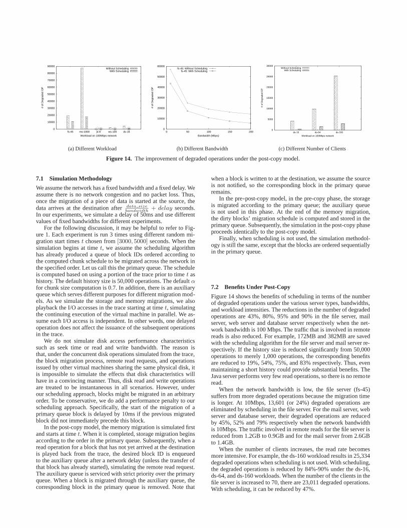
Figure 14. The improvement of degraded operations under the post-copy model.

7.1 Simulation Methodology

We assume the network has a fixed bandwidth and a fixed delay. Weassume there is no network congestion and no packet loss. Thus,once the migration of a piece of data is started at the source, thedata arrives at the destination afterdata size

bandwidth+ delay seconds.

In our experiments, we simulate a delay of 50ms and use differentvalues of fixed bandwidths for different experiments.

For the following discussion, it may be helpful to refer to Fig-ure 1. Each experiment is run 3 times using different random mi-gration start timest chosen from[3000, 5000] seconds. When thesimulation begins at timet, we assume the scheduling algorithmhas already produced a queue of block IDs ordered according tothe computed chunk schedule to be migrated across the network inthe specified order. Let us call this the primary queue. The scheduleis computed based on using a portion of the trace prior to timet ashistory. The default history size is 50,000 operations. The defaultαfor chunk size computation is 0.7. In addition, there is an auxiliaryqueue which serves different purposes for different migration mod-els. As we simulate the storage and memory migrations, we alsoplayback the I/O accesses in the trace starting at timet, simulatingthe continuing execution of the virtual machine in parallel. We as-sume each I/O access is independent. In other words, one delayedoperation does not affect the issuance of the subsequent operationsin the trace.

We do not simulate disk access performance characteristicssuch as seek time or read and write bandwidth. The reason isthat, under the concurrent disk operations simulated from the trace,the block migration process, remote read requests, and operationsissued by other virtual machines sharing the same physical disk, itis impossible to simulate the effects that disk characteristics willhave in a convincing manner. Thus, disk read and write operationsare treated to be instantaneous in all scenarios. However, underour scheduling approach, blocks might be migrated in an arbitraryorder. To be conservative, we do add a performance penalty to ourscheduling approach. Specifically, the start of the migration of aprimary queue block is delayed by 10ms if the previous migratedblock did not immediately precede this block.

In the post-copy model, the memory migration is simulated firstand starts at timet. When it is completed, storage migration beginsaccording to the order in the primary queue. Subsequently, when aread operation for a block that has not yet arrived at the destinationis played back from the trace, the desired block ID is enqueuedto the auxiliary queue after a network delay (unless the transfer ofthat block has already started), simulating the remote read request.The auxiliary queue is serviced with strict priority over the primaryqueue. When a block is migrated through the auxiliary queue, thecorresponding block in the primary queue is removed. Note that

when a block is written to at the destination, we assume the sourceis not notified, so the corresponding block in the primary queueremains.

In the pre+post-copy model, in the pre-copy phase, the storageis migrated according to the primary queue; the auxiliary queueis not used in this phase. At the end of the memory migration,the dirty blocks’ migration schedule is computed and stored in theprimary queue. Subsequently, the simulation in the post-copy phaseproceeds identically to the post-copy model.

Finally, when scheduling is not used, the simulation methodol-ogy is still the same, except that the blocks are ordered sequentiallyin the primary queue.

7.2 Benefits Under Post-Copy

Figure 14 shows the benefits of scheduling in terms of the numberof degraded operations under the various server types, bandwidths,and workload intensities. The reductions in the number of degradedoperations are 43%, 80%, 95% and 90% in the file server, mailserver, web server and database server respectively when the net-work bandwidth is 100 Mbps. The traffic that is involved in remotereads is also reduced. For example, 172MB and 382MB are savedwith the scheduling algorithm for the file server and mail server re-spectively. If the history size is reduced significantly from 50,000operations to merely 1,000 operations, the corresponding benefitsare reduced to 19%, 54%, 75%, and 83% respectively. Thus, evenmaintaining a short history could provide substantial benefits. TheJava server performs very few read operations, so there is no remoteread.

When the network bandwidth is low, the file server (fs-45)suffers from more degraded operations because the migration timeis longer. At 10Mbps, 13,601 (or 24%) degraded operations areeliminated by scheduling in the file server. For the mail server, webserver and database server, their degraded operations are reducedby 45%, 52% and 79% respectively when the network bandwidthis 10Mbps. The traffic involved in remote reads for the file server isreduced from 1.2GB to 0.9GB and for the mail server from 2.6GBto 1.4GB.

When the number of clients increases, the read rate becomesmore intensive. For example, the ds-160 workload results in 25,334degraded operations when scheduling is not used. With scheduling,the degraded operations is reduced by 84%-90% under the ds-16,ds-64, and ds-160 workloads. When the number of the clients in thefile server is increased to 70, there are 23,011 degraded operations.With scheduling, it can be reduced by 47%.

0

50

100

150

200

250

fs-45 ms-1000 js-8 ws-100 ds-16

Ext

ra tr

affic

(M

B)



Figure 15. The improvement of extra traffic under the pre+post-copy model.

0

20

40

60

80

100

120

fs-45 ms-1000 js-8 ws-100 ds-16

# of

Deg

rade

d O

P



Figure 16. The improvement of degraded operations under thepre+post-copy model.

fs-45 ms-1000 js-8 ws-100 ds-16Worst chunk size 49% 43% 49% 74% 54%performance gain

Optimal chunk size 77% 70% 64% 90% 66%performance gain

Algorithm selected 76% 50% 58% 87% 64%chunk size

performance gain

Table 4. Comparison between selected chunk size and measuredoptimal chunk size (extra traffic under pre+post-copy).

7.3 Benefits Under Pre+Post-Copy

In the pre+post copy model, the extra traffic consists of only thefinal dirty blocks at the end of memory migration. As Figure 15shows, the scheduling algorithm reduces the extra traffic in the fiveworkloads by 76%, 51%, 67%, 86% and 59% respectively.

In the pre+post copy model, the degraded operations exist onlyduring the retransmission of the dirty blocks. Since the amount ofdirty data is much smaller than the virtual disk size, the problemis not as serious as in the post-copy model. Figure 16 shows thatthe Java server, web server and database server have no degradedoperations because their amount of dirty data is small. But the fileserver and mail server suffer from degraded operations, and apply-ing scheduling can reduce them by 99% and 88% respectively.

7.4 Optimality of Chunk Size

In order to understand how optimal is the chunk size selected by thealgorithm, we conduct experiments with various manually selectedchunk sizes, ranging from 512KB to 1GB in factor of 2 increments,

to measure the performance gain achieved at these different chunksizes. The chunk size that results in the biggest performance gain isconsidered the measured optimal chunk size. The one with the leastgain is considered the measured worst chunk size. Table 4 comparesthe selected chunk size against the optimal and worst chunk sizesin terms of extra traffic under the pre+post-copy model. As can beseen, the gain achieved by the selected chunk size is greater than themeasured worst chunk size across the 5 workloads. Most of themare very close to the measured optimal chunk size.

8. SummaryMigrating virtual machines between clouds is an emerging require-ment to support open clouds and to enable better service availabil-ity. We demonstrate that existing migration solutions can have poorI/O performance during migration that could be mitigated by takinga workload-aware approachto storage migration. We develop ourinsight on workload characteristics by collecting I/O traces of fiverepresentative applications to validate the extent of temporal local-ity, spatial locality and access popularity that widely exists. We thendesign ascheduling algorithmthat exploits the individual virtualmachine’s workload to compute an efficient ordering ofchunksatan appropriate chunk size to schedule for transfer over the network.We demonstrate the improvements introduced by work-load awarescheduling on a fully implemented system for KVM and througha trace-driven simulation framework. Under a wide range of I/Oworkloads and network conditions, we show that workload-awarescheduling can effectively reduce the amount of extra traffic andI/O throttling for the pre-copy model and significantly reduce thenumber of remote reads to improve the performance of post-copyand pre+post-copy model. Furthermore, the overhead introduced byour scheduling algorithm in KVM is low.

Next, we discuss and summarize the benefits ofworkload-awareschedulingunder different conditions and workloads using the pre-copy migration model as an example.Network bandwidth: The benefits of scheduling increases as theamount of available network bandwidth for migration decreases.Given that lower bandwidth results in a longer pre-copy period,the opportunity for any content to become dirty (i.e., requiring aretransmission) is larger. However, with scheduling, content that islikely to be written is migrated towards the end of the pre-copyperiod thus reducing the amount of time and the opportunity for itto become dirty.Image size:The benefits of scheduling increases as the image size(i.e., the used blocks in the file system) gets larger even if the activeI/O working set remains the same. A larger image size results ina longer pre-copy period, thus the opportunity for any content tobecome dirty is bigger. However, with scheduling, the working setgets transferred last, reducing the probability that migrated contentbecomes dirty despite the longer migration time.I/O rate: As the I/O rate becomes more intense, the benefits ofscheduling increases. With higher I/O intensity, the probability thatany previously migrated content becomes dirty is higher. Again, bytransferring active content towards the end of the pre-copy period,we lower the probability that it would become dirty and has to beretransmitted.I/O characteristics: As the extent of locality or popularity be-comes less pronounced, the benefits of scheduling decreases. Forexample, when the popularity of accessed blocks is more uniformlydistributed, it is more difficult to accurately predict the access pat-tern. In the extreme case where there is no locality or popularitypattern in the workload, scheduling provides similar performanceto non-scheduling.

These characteristics indicate that our workload-aware schedul-ing algorithm can improve the performance of storage migrationunder a wide range of realistic environments and workloads.

References[1] Michael Armbrust, Armando Fox, Rean Griffith, and et. al. Above

the clouds: A berkeley view of cloud computing. Technical Re-port UCB/EECS-2009-28, EECS Department, University of Califor-nia, Berkeley, Feb 2009.

[2] M.G. Baker, J.H. Hartman, M.D. Kupfer, K.W. Shirriff, andJ.K.Ousterhout. Measurements of a distributed file system.ACM SIGOPSOperating Systems Review, 25(5):212, 1991.

[3] M. Blaze. NFS tracing by passive network monitoring. InProceedingsof the USENIX Winter 1992 Technical Conference, pages 333–343,1992.

[4] ”Amazon Web Services Blog”. Animoto - Scaling Through ViralGrowth. http://aws.typepad.com/aws/2008/04/animoto—scali.html,April 2008.

[5] Robert Bradford, Evangelos Kotsovinos, Anja Feldmann, and HaraldSchioberg. Live wide-area migration of virtual machines includinglocal persistent state. InACM/Usenix VEE, June 2007.

[6] Christopher Clark, Keir Fraser, Steven Hand, Jacob GormHansen,Eric Jul, Christian Limpach, Ian Pratt, and Andrew Warfield. Livemigration of virtual machines. InNSDI’05: Proceedings of the 2ndconference on Symposium on Networked Systems Design & Implemen-tation, pages 273–286, Berkeley, CA, USA, 2005. USENIX Associa-tion.

[7] M.D. Dahlin, C.J. Mather, R.Y. Wang, T.E. Anderson, and D.A. Pat-terson. A quantitative analysis of cache policies for scalable networkfile systems. ACM SIGMETRICS Performance Evaluation Review,22(1):150–160, 1994.

[8] Derek Gottfrid. The New York Times Archives + AmazonWeb Services = TimesMachine. http://open.blogs.nytimes.com/2008/05/21/the-new-york-times-archives-amazon-web- services-timesmachine/, May 2008.

[9] James Hamilton. The Cost of Latency.http://perspectives.mvdirona.com/2009/10/31/ TheCostOfLa-tency.aspx, October 2009.

[10] Michael R. Hines and Kartik Gopalan. Post-copy based live vir-tual machine migration using adaptive pre-paging and dynamic self-ballooning. In VEE ’09: Proceedings of the 2009 ACM SIG-PLAN/SIGOPS international conference on Virtual execution environ-ments, 2009.

[11] Takahiro Hirofuchi, Hidemoto Nakada, Hirotaka Ogawa, Satoshi Itoh,and Satoshi Sekiguchi. A live storage migration mechanism over wanand its performance evaluation. InVIDC’09: Proceedings of the 3rdInternational Workshop on Virtualization Technologies inDistributedComputing, Barcelona, Spain, 2009. ACM.

[12] Takahiro Hirofuchi, Hirotaka Ogawa, Hidemoto Nakada, Satoshi Itoh,and Satoshi Sekiguchi. A live storage migration mechanism over wan

for relocatable virtual machine services on clouds. InCCGRID’09:Proceedings of the 2009 9th IEEE/ACM International Symposiumon Cluster Computing and the Grid, Shanghai, China, 2009. IEEEComputer Society.

[13] Hai Jin, Li Deng, Song Wu, and Xuanhua Shi. Live virtual machinemigration integrating memory compression with precopy. InIEEEInternational Conference on Cluster Computing, 2009.

[14] KVM. QEMU-KVM code. http://sourceforge.net/projects/kvm/files,January 2010.

[15] Yingwei Luo, Binbin Zhang, Xiaolin Wang, Zhenlin Wang,YifengSun, and Haogang Chen. Live and Incremental Whole-System Migra-tion of Virtual Machines Using Block-Bitmap. InIEEE InternationalConference on Cluster Computing, 2008.

[16] Open Cloud Manifesto. Open Cloud Manifesto.http://www.opencloudmanifesto.org/, January 2010.

[17] Michael Nelson, Beng-Hong Lim, and Greg Hutchins. Fast transparentmigration for virtual machines. InUSENIX’05: Proceedings of the2005 Usenix Annual Technical Conference, Berkeley, CA, USA, 2005.USENIX Association.

[18] J.K. Ousterhout, H. Da Costa, D. Harrison, J.A. Kunze, M. Kupfer,and J.G. Thompson. A trace-driven analysis of the UNIX 4.2 BSDfilesystem.ACM SIGOPS Operating Systems Review, 19(5):24, 1985.

[19] K.K. Ramakrishnan, Prashant Shenoy, and Jacobus Van derMerwe.Live data center migration across wans: A robust cooperativecontextaware approach. InACM SIGCOMM Workshop on Internet NetworkManagement (INM), Kyoto, Japan, aug 2007.

[20] IBM Redbooks.IBM Powervm Live Partition Mobility IBM Interna-tional Technical Support Organization. Vervante, 2009.

[21] D. Roselli, J.R. Lorch, and T.E. Anderson. A comparison of file systemworkloads. InProceedings of the annual conference on USENIXAnnual Technical Conference, page 4. USENIX Association, 2000.

[22] Franco Travostino, Paul Daspit, Leon Gommans, Chetan Jog, Ceesde Laat, Joe Mambretti, Inder Monga, Bas van Oudenaarde, SatishRaghunath, and Phil Yonghui Wang. Seamless live migration of virtualmachines over the man/wan.Future Gener. Comput. Syst., 22(8):901–907, 2006.

[23] VMWare. VMmark Virtualization Benchmarks.http://www.vmware.com/products/vmmark/, January 2010.

[24] Timothy Wood, Prashant Shenoy, Alexandre Gerber, K.K. Ramakr-ishnan, and Jacobus Van der Merwe. The Case for Enterprise-ReadyVirtual Private Clouds. InProc. of HotCloud Workshop, 2009.

[25] Timothy Wood, Prashant Shenoy, Arun Venkataramani, and MazinYousif. Black-box and gray-box strategies for virtual machine mi-gration. InNSDI, 2007.

[26] XEN. XEN Project. http://www.xen.org, January 2009.

Workload-Aware Live Storage Migration for Clouds

Documents

Transcript of Workload-Aware Live Storage Migration for Clouds