Working Paper -

I

Adaptive Optimization for Forest-Level Timber Harvest

Decision Analysis

Peichen Gong

WP-92-70 September 1992

BIIASA International Institute for Applied Systems Analysis A-2361 Laxenburg D Austria

Telephone: +43 2236 715210 Telex: 079 137 iiasa a o Telefax: +43 2236 71313

Adaptive Optimization for Forest-Level Timber Harvest

Decision Analysis

Peichen Gong

WP-92-70 September 1992

Working Papers are interim reports on work of the International Institute for Applied Systems Analysis and have received only limited review. Views or opinions expressed herein do not necessarily represent those of the Institute or of its National Member Organizations.

International Institute for Applied Systems Analysis o A-2361 Laxenburg Austria

Telephone: +43 2236 715210 Telex: 079 137 iiasa a o Telefax: +43 2236 71313

Abstract

This paper describes a method for optimizing multistand timber harvest decisions under

uncertainty. The optimal decision policy is approximated by a timber supply function. The

supply function is formulated analytically and the supply function coefficients are optimized

numerically by maximizing the expected present value of the forest. This method is

implemented to the problem of timber harvest decision making under timber price uncertainty

for a simple forest with one forest-level activity, i.e., investment in timber harvest capacity,

incorporated. Stochastic quasigradient methods are introduced and suggested to be used to

optimize the supply function coefficients. Advantages of this method lie in its computational

efficiency, flexibility of model formulation, and its application potentials. A numerical

example is used to illustrate the application of this method. Sensitivity analysis shows that

the level of timber price uncertainty affects both the optimal harvest decision policy and the

expected present value of the forest. However, the effects of correlations between timber

prices in successive periods are not obvious, probably because of the relatively long decision

intervals used in this study. Comparison of the numerical results with the optimal solution

to a corresponding deterministic linear program shows that substantially higher expected

present value of the forest (12.5-88.4% higher than the linear programming solution,

depending on the variance and correlation of the timber price process) can be obtained using

this method with the currently formulated timber supply function structure.

KEY WORDS: Forest management, supply function, uncertainty, stochastic optimization.

Acknowledgements

This is an extended version of an earlier paper entitled "A model for forest level adaptive

timber harvest decisionsn. The study reported in this paper was started in IIASA when I

participated the IIASA Young Scientists' Summer Program 1991. I would like to thank Yuri.

Kaniovski for continuous and encouraging discussions, and R. J-B Wets, P. Lohmander, D.

P. Dykstra, D. Carlsson and P. Fredman for helpful comments. This research was supported

by the Swedish Council for Planning and Coordination of Research (FRN) and the Swedish

Council for Forestry and Agricultural Research (S JFR) .

Contents

1 . Introduction

2. The Problem and the Proposed Method

2.1 The problem

2 .2 The proposed method

3. The Model and Solution Methods

3.1 The timber supply function

3.2 The objective function

3.3 Solution methods

4. A Numerical Example

5. Model Improvements and Extensions

6 . Summary and Discussions

References

Adaptive Optimization for Forest-Level

Timber Harvest Decision Analysis

Peichen Gong

1. Introduction

To date, deterministic optimization techniques, especially deterministic linear programming,

are commonly used in timber harvest decision analysis. While deterministic timber harvest

scheduling techniques have been continuously improved, they usually can not explicitly

recognize and appropriately incorporate uncertainty in the future forest-market state in timber

harvest decision analysis. Uncertainty in forest management has been widely acknowledged,

and it has been argued that since the decision maker does not have perfect knowledge about

the future, uncertainty in the future forest-market state should be explicitly taken into account

in decision analysis (Buongiorno and Kaya, 1988; Smith, 1988). The theory of decisions

under risk (uncertainty) was introduced into forestry (see, e.g., Thompson, 1968), and a

number of studies have been conducted to investigate the applicability of various decision

methods to forest management (timber harvest) decision analysis under uncertainty.

Hool(1966) applied a Markov chain approach to an optimal forest production control (timber

harvest) problem under forest stand state uncertainty. This approach was later applied to the

management of even-aged (Lembersky and Johnson, 1975) and uneven-aged stand (Kaya and

Buongiorno, 1987), where both timber price and timber growth are stochastic. Lohmander

(1988b) studied the optimal stopping rule in even-aged stand management and derived the

optimal reservation prices for clear cutting decisions. Similar problems were also studied by

Brazee and Mendelsohn (1988) and Gong (1991). Effects of the risk of forest destruction

caused by catastrophic reasons, such as fire, on the optimal rotation of a forest stand were

investigated by, among others, Martell (1980), Routledge (1980), Reed (1984), and Caulfield

(1988). Gong (1992) applied a multiobjective dynamic programming method to a timber

harvest decision problem when nontimber values of the stand is considered.

The results of these studies are promising. Several methods, such as Markov chain approach,

stochastic dynamic programming, stochastic dominance analysis, etc., have been successfully

applied to the respective example problems. However, all these studies are focused on stand-

level decision analysis. More than often, timber harvest decisions for the individual stands

in a forest can not be made independently. Possible reasons for the interdependencies

between the timber harvest decisions for the individual stands include

(1) Imperfect decision environment: Timber supply from a specific forest could be so

important to the market that timber price is no longer exogenous to the harvest

decisions; Budget and harvest-flow constraints are often imposed, especially in the

management of public forests; The size of continuous clear cutting area is sometimes

regulated;

(2) Considerations of nontimber benefits of the forest (the multiple-use problem);

(3) Nonlinear timber harvest cost functions;

(4) Timber harvest related forest-level activities, such as investment in harvest capacity

and road construction;

(5) Ecological interactions between the stands.

Under such circumstances, the overall timber harvest decision for a forest, formed by

aggregating (putting together) the independently made decisions for the individual stands

within the forest, could be either infeasible or not optimal. Methods which have been used

in previous studies for stand-level management (timber harvest) decision analysis under

uncertainty in timber price and/or timber growth commonly require solving recursive

equations numerically to identify the optimal decision policy. Unfortunately it is difficult to

apply these methods, which are applicable to stand-level decision analysis, to analyze the

problem of multistand timber harvest decisions under uncertainty appropriately because of

the well-known dimensionality problem. Lohmander (1988a) conducted an analytical study

of the problem of continuous extraction (harvest) of the renewable resource under uncertainty

in the price and growth of the resource. The (comparative static) results derived are

important, yet the explicit optimal harvest policy can not be obtained analytically.

Hoganson and Rose (1987) presented a timber management scheduling model which

incorporates forestwide uncertainty. In this model, the planning horizon is divided into two

parts, the "short-run" when the state of nature is known with certainty and the "long-run"

in which the state of nature is stochastic. Uncertainty in the "long-run" is described by a

number of scenarios, and the model is formulated in such a way that harvest schedules in the

"long-run" are distinguished between the scenarios, while the "short-run" activities are

identical no matter what specific scenario takes place in the future. An improvement of this

model over the deterministic ones is that, in making the current decisions, a number of

possible states of nature in the future are explicitly recognized and taken into account.

However, such a formulation assumes that the actual state of nature in all the future periods

(the realized scenario) can be completely observed in the beginning of the second part of the

planning horizon. It is obvious that a "scenario" recognized in this model consists of the state

of nature in a number of sequential decision periods and is only partly revealed after the

observation in each single period has been made. While extension of this model to recognize

the sequential structure of uncertainty and to incorporate the observations made in different

decision periods is not practical because of computational reasons, such a simplification of

the information (observation) structure will in principle result in over estimation of the

expected present value of the net revenues in the future periods.

Thompson and Haynes (1971) proposed a "partially stochastic linear programming" approach

for analyzing decisions under uncertainty, and applied it to a wood procurement problem of

a forest industry firm. This approach consists of two steps. First, simulate the possible states

of nature in the future by using (subjective) probability distributions of the random state

variables. Second, solve the linear program for each and every simulated state of nature. This

method would be appropriate for analyzing the problem of decision making under uncertainty

when perfect information could be available (at some cost).

Reed and Emco (1986) incorporated the risk of forest fire in a timber harvest scheduling

model. The optimal decision is identified by solving a deterministic linear programming

problem which approximates the original stochastic one. The applicability of this method,

however, is limited to this special kind of uncertainty. When uncertainty in other factors,

such as timber price, is present, it is in general impossible to find an equivalent deterministic

problem as long as one does not exclude the adaptive mechanism from the model.

The main difficulty of incorporating uncertainty in forest-level timber harvest decision

analysis by extending deterministic timber harvest scheduling models is that the resulted

optimization problem is (numerically) too complicated to be solvable. This paper presents an

alternative approach to formulate and solve the problem of forest-level timber harvest

decision making under uncertainty. With this approach, the adaptive mechanism can be

incorporated into a solvable forest-level timber harvest decision model without simplifying

the sequential structure of uncertainty in the future state of nature. To be specific, the fact

that observations of the realized state of nature are made sequentially is recognized and the

dependency of the optimal harvest level in the future periods on the then observed state of

nature is explicitly formulated in the decision model, while keeping the model manageable

(solvable). After a brief description of the problem addressed and the proposed approach for

formulating and solving the problem, the decision model is formulated and solution methods

are discussed followed by an introduction to stochastic quasigradient methods which will be

used to solve the optimization problem. The formulated decision model and the introduced

solution method are applied to a numerical example problem, and comparison of this model

with the deterministic linear programming method is conducted. Possible improvements and

extensions of the described model for more complex decision problems, aa well as the

efficiency of this approach are discussed.

2. The Problem and the Proposed Method

2.1 The problem

We are thinking of the problem of forest-level timber harvest decision making under

uncertainty. The sate of the forest in period t is described by X, and V.

where N is the maximum relevant age (in number of age-classes) of the stands, x: (for i= 1,

. . . , N) is the area of the stands in age-class i in period t, and v i is the per unit area growing

stock of timber in age-class i. V is constant over time.

Timber price in the future is stochastic and the stochastic timber price process can be

estimated from historical timber price records. The timber market is perfect and the actual

timber price in any period can be observed before the decision for that period has to be

taken. The management objective is maximizing the expected present value of the net

revenues in the current and in all the future periods. Decisions are related to the optimal

timber harvest level.

Previous studies of stand-level timber harvest decision problems show that, when timber

price is stochastic, the expected present value of a forest stand could be increased

significantly if observations of the actual timber price in the future periods are utilized and

decisions are taken adaptively (Brazee and Mendelsohn, 1988; Lohmander, 1988b). When

timber harvest decisions should be made at forest-level, there are two connected questions

to ask. (1) Can we find a computationally feasible method for forest-level timber harvest

decision analysis under uncertainty? And (2) if we can, is the method efficient? In other

words, can the expected present value of the forest be increased when the identified method

is used to explicitly take into account uncertainty in timber harvest decision making?

This study is mainly concerned with the first question. The objective is to develop a method

which enables the adaptation of future timber harvest decisions to the observed timber prices

without over-simplifying the structure of the problem. To highlight the development of the

method, we consider a forest with one tree species and one site quality. One forestwide

activity, i.e., investment in timber harvest capacity, is considered. As to the second question,

the answer could be affected by how the method is used. And it is likely that the magnitudes

of changes in the expected present value resulting from the use of a new decision method are

problem dependent. For these reasons we do not intend to draw any general conclusion with

respect to the second question.

2.2 The proposed method

Generally spealong, forest management is a multistage decision problem where the optimal

decisions in the current period and in all the future periods are interdependent. It is therefore

essential to consider also decisions in the future periods when making the decision related

to the management activities in the current period. Moreover, the optimal decision in every

period is dependent on the forest-market state in the same period which is affected by

decisions in the preceding periods and by a number of random factors. Since the forest-

market state in the future periods is not known with certainty, uncertainty should be taken

into account and decisions in the future periods should be formulated appropriately. When

decisions are made at stand-level, the scale of the problem is relatively small and it is usually

possible to formulate and determine the optimal decisions for each and every possible stand-

market state in the future periods. In this case, the dependency of the optimal decision on the

stand-market state is formulated implicitly and the optimal decision policy is derived

explicitly. Forest-level decision problems are much more complicated in terms of the

decision- and the state-space. It is generally impossible to derive the optimal decision for

each and every possible forest-market state directly because of the enormous number of

possible states and decisions which should be considered. In such cases, one may think of

the possibility of using some function to describe the dependency of the optimal decision on

the state of nature, and deriving the optimal decision for each possible state of nature

indirectly by optimizing the structure and coefficients of this function. By this means the

problem can hopefully be made manageable. Clearly, the obtained optimal function is an

approximation of the true optimal decision policy.

In timber harvest decisions, such a function should link the optimal harvest level with the

forest-market state variables which affect the harvest decisions. This leads us to think of the

timber supply function. From production theory, the supply function of a firm is a functional

relation between the optimal production level and prices of the product and the production

factors conditional on the production conditions (e.g., technology, capacity, etc.). Once such

a supply function has been obtained, the optimal production level can be easily determined

after the actual prices have been observed. Following this idea, the method which is proposed

for forest-level timber harvest decision analysis is to derive the (short-run) timber supply

function of the forest. The structure of the timber supply function can be formulated

analytically, and the supply function coefficients are optimized numerically by maximizing

the expected present value of the current and all the future net revenues when timber harvest

decisions will be made by using this supply function.

With such a representation of the timber harvest decision policy, the problem of forest-level

timber harvest decision making 'under uncertainty can be formulated as a single-stage

stochastic optimization problem. In this way we overcome the dimensionality problem, which

seems to be the main obstacle for the application of stochastic models to forest-level timber

harvest decision analysis. Uncertainty in timber price, in the forest state (forest state

transitions), and in timber harvest cost can be simultaneously incorporated into the decision

model. And as it will be shown, such a method is quite flexible in the sense that constraints

related to the periodic timber harvest level can be easily accommodated in the model and that

this method is capable of dealing with "nonstandard" timber harvest decision problems in

which the timber harvest cost function is nonlinear and/or the timber market is not perfectly

competitive.

3. The Model and Solution Methods

The best way to describe and discuss this method in more detail is to use it to formulate and

solve a concrete timber harvest decision problem. In this Section, we formulate a timber

supply function and the stochastic optimization problem related to the timber harvest decision

problem which was described in Section 2. Then solution methods which can be used to

solve the obtained optimization problem will be introduced.

3.1 The timber supply function

To implement this method, we first need to find a suitable structure for the timber supply

function. Theoretically, the supply function of a firm can be derived from the profit function

of production. However, the timber supply function can rarely be obtained in this way

because the profit function (the maximum present value function) can not be formulated

explicitly due to the multistage nature of timber harvest decision problems. Although there

are analyses about the properties of the implicit timber supply function in deterministic or

stochastic contexts (Johansson and Liifgren, 1985; Lohmander, 1988a), there is no analytical

discussion, to the best of my knowledge, about the appropriate structure of the timber supply

function in the literature. There are, however, a number of econometric studies of the timber

harvest behavior of nonindustrial private forest (NIPF) owners (Kuuluvainen, 1989;

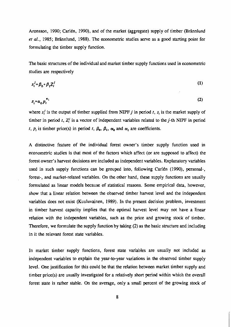
Aronsson, 1990; CarlCn, 1990), and of the market (aggregate) supply of timber (Brhnlund

et al., 1985; Briinnlund, 1988). The econometric studies serve as a good starting point for

formulating the timber supply function.

The basic structures of the individual and market timber supply functions used in econometric

studies are respectively

where s j is the output of timber supplied from NIPF j in period t, s, is the market supply of

timber in period t, Zj is a vector of independent variables related to the j-th NIPF in period

t, p, is timber price(s) in period t, Po, P,, a, and a, are coefficients.

A distinctive feature of the individual forest owner's timber supply function used in

econometric studies is that most of the factors which affect (or are supposed to affect) the

forest owner's harvest decisions are included as independent variables. Explanatory variables

used in such supply functions can be grouped into, following CarlCn (1990), personal-,

forest-, and market-related variables. On the other hand, these supply functions are usually

formulated as linear models because of statistical reasons. Some empirical data, however,

show that a linear relation between the observed timber harvest level and the independent

variables does not exist (Kuuluvainen, 1989). In the present decision problem, investment

in timber harvest capacity implies that the optimal harvest level may not have a linear

relation with the independent variables, such as the price and growing stock of timber.

Therefore, we formulate the supply function by taking (2) as the basic structure and including

in it the relevant forest state variables.

In market timber supply functions, forest state variables are usually not included as

independent variables to explain the year-to-year variations in the observed timber supply

level. One justification for this could be that the relation between market timber supply and

timber price(s) are usually investigated for a relatively short period within which the overall

forest state is rather stable. On the average, only a small percent of the growing stock of

timber (or forest area) is harvested in each year. Effects of timber harvest on the

development of the aggregate (overall) forest state are small in a relatively short period.

However, the same can not be said of the individual forests. Annual (or periodic) timber

harvest level in a single forest could be high enough to change the forest state significantly,

which in turn affects harvest decisions in the subsequent periods. The forest state, therefore,

should be explicitly included in the timber supply function of a specific forest.

Effects of the forest state on the optimal timber harvest level could be taken into account in

several ways, for example, by including the forest area in each age-class or some aggregate

measurets) of the forest state in the supply function. In this study, we take into account a

lower age limit when clear cutting is allowed. Two aggregate forest state variables, the total

and the average per unit area growing stock of timber in the harvestable stands (stands which

are not younger than the lower age limit) in the forest, are used to reflect the supply effects

of the forest state. The total growing stock of timber determines the harvest potential (the

highest possible harvest level) in each period. However, a change in the total growing stock

of timber may result from changes in the harvestable area and/or in the average per unit area

volume, both of which are important for the determination of the optimal harvest level. Since

the harvestable area can be uniquely determined when the total and the average per unit area

growing stock in timber of the harvestable stands are known, we choose the latter two as

independent variables in the timber supply function. The average per unit area volume

reflects effects of the average age of the harvestable growing stock of timber on the optimal

harvest level.

Including these two independent variables, the supply function is formulated as

where S, is the amount of timber supplied from the forest under consideration in period t, Y,

is the harvestable growing stock of timber in period t, A, is the average per unit area volume

in period t, at,,-% are coefficients. Y, and A, are calculated by

where z is the lower age limit (in number of age-classes) when clear cutting is allowed.

With supply function (3), the timber harvest level will be continuously adjusted according

to the observed timber price and forest state. Though this is an improvement over the

deterministic timber harvest scheduling formulations where only one of all the possible

timber price series in the future periods can be recognized and possible adjustments of the

optimal harvest level in the future periods can not be incorporated in the model. However,

the adjustment of harvest level to timber price in supply function (3) is not always sufficient.

When the observed timber price is low enough in some period, it is possible that to wait one

period for a possibly higher price is more profitable than harvest anything at all in that

period. In such a case, the supply of timber (harvest level) should be reduced to zero instead

of some lower level calculated by using (3). To incorporate such discontinuous adjustments

of the harvest level, we introduce a reservation price in the supply function. The reservation

price RP, is formulated as a function of the average volume per unit area.

where a,-a, are coefficients.

Including this reservation price in (3), the supply function is

In addition to timber price and the forest state, there are several other factors, such as the

personal-related variables and timber harvest cost, which affect the optimal timber harvest

level, as has been mentioned earlier. When analyzing the timber harvest decision problem

related to a specific forest and the management objective is maximizing the expected present

value, the personal-related variables are (or can be regarded as) constant, and therefore need

not be explicitly included in the supply function. Timber harvest cost can be explicitly

included in the timber supply function, and uncertainty in timber harvest cost in the future

periods can be taken into account directly in optimization of the supply function coefficients.

When timber harvest cost function is linear and when the correlation between prices and the

correlation between (per cubic meter) harvest costs in successive periods are of the same

sign, the effect of an increase in timber harvest cost on the optimal harvest level is similar

to that of a decrease in timber price. It is then possible to take into account uncertainty in

timber harvest cost indirectly by using the net timber price in the supply function. We

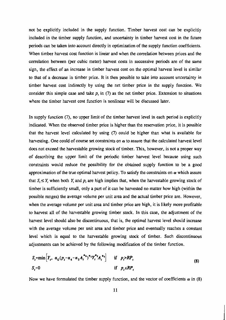
consider this simple case and take p, in (7) as the net timber price. Extension to situations

where the timber harvest cost function is nonlinear will be discussed later.

In supply function (7), no upper limit of the timber harvest level in each period is explicitly

indicated. When the observed timber price is higher than the reservation price, it is possible

that the harvest level calculated by using (7) could be higher than what is available for

harvesting. One could of course set constraints on ar to assure that the calculated harvest level

does not exceed the harvestable growing stock of timber. This, however, is not a proper way

of describing the upper limit of the periodic timber harvest level because using such

constraints would reduce the possibility for the obtained supply function to be a good

approximation of the true optimal harvest policy. To satisfy the constraints on ar which assure

that S, I Y, when both Y, and p, are high implies that, when the harvestable growing stock of

timber is sufficiently small, only a part of it can be harvested no matter how high (within the

possible ranges) the average volume per unit area and the actual timber price are. However,

when the average volume per unit area and timber price are high, it is likely more profitable

to harvest all of the harvestable growing timber stock. In this case, the adjustment of the

harvest level should also be discontinuous, that is, the optimal harvest level should increase

with the average volume per unit area and timber price and eventually reaches a constant

level which is equal to the harvestable growing stock of timber. Such discontinuous

adjustments can be achieved by the following modification of the timber function.

Now we have formulated the timber supply function, and the vector of coefficients ar in (8)

will be optimized by maximizing the expected present value of the forest. Before turning the

discussion to the expected present value function, we first examine the constraints on ar. The

sign of each element of ar can be determined by the signs of timber supply S, and the

reservation price RP,, and by the signs of their (partial) derivatives with respect to the

relevant variables. Timber supply S, is always nonnegative and sometimes strictly positive,

it follows that > 0. Previous studies show that as, lap, > 0 and as, lax > 0 (Johansson and

Liifgren, 1985; Lohmander, 1988a), from which a, and a, should be positive. Since the term

A, represents the average age of the harvestable growing stock of timber, it is reasonable to

assume that the optimal harvest level does not decrease with A,, i.e., ar320. And from the

fact that the optimal reservation price decreases with stand age1, aRPIaA, < 0, the signs of

as and ar, should be opposite, i.e., %*u6< 0. We choose us> 0 and ar6<0, and a, is

restricted to be nonnegative because the optimal reservation price can not be negativs. Since

the upper and lower bounds of the periodic timber harvest level have been included in the

supply function and with the above restrictions on the signs of ar4-ar, the reservation price is

always positive, no explicit constraint on the absolute values of ar,-a, is necessary.

3.2 The objective function

Having formulated the structure of the timber supply function, the coefficients should be

optimized before we can use the supply function to make harvest decisions. This is done by

maximizing the expected present value of the forest, i.e., the expected present value of the

net revenues of timber harvest and investments in the current and all the future periods. To

formulate the expected present value function, we make the following specifications of the

problem: Harvesting takes place in the beginning of the decision period and the harvested

area will be planted immediately with the same tree species at a constant per unit area

At forest-level this should also be true, though the optimal reservation price curve of

a forest may be different from that of a single stand.

The discussion about the signs of ar is for the purpose of setting up lower (upper) bonds

for the individual coefficients, which is desirable for the optimization process (Gaivoronski,

1988b). The example test show that, even if these constraints are removed, the obtained

optimal value of ar still fall in these regions, and therefore support the above arguments.

12

planting cost; Investment in timber harvest capacity in any period, if necessary, is made just

before harvesting in the same period takes place; Investment in timber harvest capacity is

continuous and the unit investment cost is constant. Given the supply function coefficients

a , the expected present value function has the following form,

where F(a) is the expected present value of the forest, E stands for mathematical expectation,

JT * ) is the random present value function with a particular realization of the price process P

when the harvest policy defined by (8) is followed, &-, is the initial age-class distribution of

the forest, K, is the initial timber harvest capacity, n is the number of years included in one

decision period, T is the number of decision periods considered, R, is the net revenue of

timber harvest in period t, CP is the cost incurred by planting the harvested area in period

t, C: is the cost of investment in timber harvest capacity in period t, Ilf is the present value

of the ending forest, and IIK is the present value of the ending timber harvest capacity.

Age-Class Specflcation of the Periodic Harvest Volume: In order to calculate the harvested

area in each period and to determine the forest state in the subsequent period, the periodic

harvest volume determined by using the timber supply function should be allocated to the

age-classes. To do this, we adopt a simple rule of cutting from the oldest to the younger age-

classes. There are other ways of allocating the periodic harvest, some of which may be better

than the one used here in the sense that more detailed forest state information can be utilized.

However, the "oldest cut first" rule is simple to use and therefore enables us to highlight the

formulation of the optimization problem and to concentrate on the solution methods. The

solution methods which will be introduced are also applicable when other timber harvest

allocating methods are used, using a more complicated method to determine the harvest area

in each age-class does not help to gain more insights of the problem. Let ~,=(h,', h:, ..., hITT denote the vector of harvest area in period t, HI should satisfy the following constraints.

(1) The area constraint:

HtsX, for t=1, ..., T

(2) The total harvest volume constraint:

VH,=S, for t=1, ... , T

From these constraints on H, and the cutting rule we setup, the total harvest volume in period

t can be allocated to the age-classes by the following set of equations.

N

( s t - x h:vj)/v for i=N-1, N-2, ... , z j=i+l

h : = ~ for i= l , ..., z-1 (10~)

The total area harvested in period t is

Forest State Tmnsition: Since the forest state is described by the area in each age-class,

forest state transitions can be formulated in the following way.

where G,' and G: are the transition matrices.

where g( is the portion of area in age-class i in period t, i.e., x(-h(, moving up to age-class

i+ 1 in period t+ 1. In the simplest case when the decision period length is equal to the age-

class width, g(= 1 for all i and t.

Investment in nmber Harvest Capacity: Investment in timber harvest capacity is determined

in the following way: Investment in any period is made only if the existing capacity falls

short of the harvest requirement, and the investment will not exceed what is necessary in the

same period.

It== [0, St-Kt] (13)

where K, is the existing timber harvest capacity in the beginning of period t before investment

in the same period has been made.

nmber Harvest Capacity Tmnsition: From the above investment rule, the existing timber

harvest capacity in a period (i.e., timber harvest capacity carrying over from the preceding

periods) is one variable which affects the investment level in that period. To formulate the

dynamics of timber harvest capacity, it should be noted that the machines purchased in one

period are unlikely to be completely out of use in the next period, nor is it true that they can

be used forever without reduction in productivity. When the time horizon considered is long,

which it usually is, proper accounting of harvest capacity is especially important. We assume

that the productivity of the machines decreases over time exponentially at a constant rate A,

and the dynamics of the timber harvest capacity is

Kl =KO

K,=(K,-,+I~-~)~-" for t=2 ,..., T+l

Revenues and Costs: The periodic revenues and costs within time horizon T can now be

explicitly formulated.

Timber harvest revenue: R, =P,S, (15)

Planting cost: cp=cl~,C (16)

hvestment cost: c;=c2It (17)

where C and C are respectively the per unit area regeneration cost and the price of timber

harvest capacity.

End Values: The expected present value of the ending forest is estimated using Faustmann

forest (land) expectation values, i.e., the expectation value of the forest land when there are

trees of age t (Johansson and Liifgren, 1985). The present value of the ending timber harvest

capacity is equal to its market value (in present term).

where w=(wl, g,. . . , )cT) is a vector of Faustmann forest expectation values.

Substitute (15)-(19) into (9), the expected present value function is

where the harvest level S,, harvested area A:, the forest state XI, investment in timber harvest

capacity I,, and the timber harvest capacity K,, have been defined in (4), (5) , (8), (lOa),

(lob), (1W, (111, (121, (13), and (14).

3.3 Solution methods

The resulting optimization problem is

Find acQcRm

such that F(a) =E Lf(a, X,, K& P)] is maximized

where Q refers to the feasible set of the coefficient vector a in timber supply function (8),

m is the dimension of a (the number of supply function coefficients).

This is a stochastic optimization problem, for which several solution methods are available

(Ermoliev and Wets, 1988). The main difficulty of using algorithms developed for

deterministic problems to solve (21) is the need of calculating the mathematical expectation.

Because of the dynamics involved in the random functionfl-) and the possible correlations

between timber prices in successive periods, the objective function F(a) and its gradients can

not be calculated directly. Stochastic optimization techniques are designed precisely to

overcome this difficulty. There are two basic types of stochastic optimization methods, i.e.,

approximation methods (Wets, 1983) and stochastic quasigradient methods (Ermoliev, 1983).

In the remainder of this Section we give a brief introduction to stochastic quasigradient

methods which will be used later on to solve the example problem. For detailed discussions

about the theoretical and implementation aspects of the method, the readers are referred to

Ermoliev (1983, 1988) and Gaivoronski (1988a, 1988b).

Consider the following maximization problem

Find xcXcRn

such that F(x) =E lf(x, o)] is maximized

wherex is the vector of decision variables and w the vector of random parameters. Stochastic

quasigradient methods solve problem (22) through an iterative procedure which utilizes

samples of the random function flx, a). The iterates are obtained by

where p j , means projection on X, p' is step size, and (' is step direction.

The step direction (' is determined by the stochastic quasigradients of function F(x) which

can be obtained by the sample gradients (subgradients) of the random functionflx, a). The

simplest way of choosing step direction is

tS=f,(xS, .r') (23b)

where d is a sample of the random parameter o.

If taking a sample of the random parameter o and calculating the gradients (subgradients) of

the random function flx, o) is inexpensive (in terms of CPU time), one could take the

average of some specified number L of samples of the gradients (subgradients) of the random

function flx, o) .

where ol.. .d are independent samples of o.

Starting from an initial point xO, in each iteration s, one (or L) sarnple(s) of the random

parameter o are taken and the gradients (subgradients) and the value of functionflx, o) are

calculated at xs. The direction of movement from xs is determined by using (23b) or (23c),

and a new vector of values of the decision variable xS+' are obtained from (23a). The process

is continued from xs+' on, until xS+' approaches the optimal point x'.

4. A Numerical Example

The timber supply function constructed and the solution method outlined in the preceding

Section are applied to a hypothetical timber harvest decision problem to illustrate how the

proposed method may work numerically. The forest consists of stands of Pinus contorta with

the same site quality, and the initial age-class distribution of the forest is given in Table 1.

Table 1. The initial forest state.

age-class

area (ha) 820 820 820 820 820 820 820 825

The maximum relevant stand age (in age-classes) N is 20, but there is no stand older than

8 in the initial forest. The per hectare timber volume in age-class i (for i= 1, 2, . . . , N) is

estimated with the following yield function (Fridh and Nilsson, 1980).

The net timber price follows an AR(1) process.

where 4,,=20.0 and 4,=0.8, the random term e, for all t are independent, normally

distributed with zero mean and standard deviation a,= 15.0.

The initial timber harvest capacity is 0.00 m3, investment cost per unit harvest capacity is

100.00 Swedish crowns (SEK) per cubic meter, the rate of decrease of timber harvest

capacity is 4%, planting cost is 1000.00 SEWha, and a continuous real discount rate of 3%

is used. Forty five-year decision periods are included in the expected present value function

(the objective function). The minimum stand age when clear cutting is allowed is set equal

to 6.

Seven coefficients in the timber supply function (8) need be optimized. Preliminary runs of

the optimization program show that if the value of is fixed in the optimization process the

optimal values of a0-a5 can be obtained much more quickly?. We tested three fixed values

of a6, i.e., the coefficients q,-ar, are optimized in three cases when a,=-1 .O, as=-0.5, and

when a6=0 (here zero can be viewed as the maximum value of 4. The results show that

When %-a6 are optimized simultaneously, the required number of iteration increases.

The main reason is that step size p' is controlled subjectively and we did not implement any

formal rule of choosing step size in the optimization program.

the expected present value of the forest is rather insensitive to the value of a6 (see Table 2),

and therefore optimization of %-a, with other values of a, are omitted.

The optimal value of the supply function coefficients are also derived for four other timber

price process scenarios, partly to show the effects of timber price uncertainty (measured by

the standard deviation of the random term e, in the price process (24)), and partly to

investigate the effects of correlations between timber prices in successive periods. The four

tested price process scenarios are

(1) p1=20.0+0.8p,, +e; u,=25.0

(2) pl=2O.0+O.8p,,+e; u,=5.0

(3) pl=60.0+O.4p,,+e; u,=22.9129

(4) p,= lOO.O+e; u,=25.0

For an AR(1) process, a change in the value of 4, not only changes the autocorrelation

function of the process, it also changes the mean and the (unconditional) variance of the

process. The indirect changes in the mean and the variance likely affect the optimal harvest

policy and/or the expected present value of the forest, and therefore could mask the effects

of timber price correlation. For this reason, the values of 4, and u, in scenarios (3) and (4)

are changed correspondingly to keep the mean and the variance of the process constant.

The optimal solution to the example problem is presented in Table 2. The last row in Table

2 gives the estimated expected present value of the forest. Estimates of the expected present

value of the forest in Table 2 through Table 4 are obtained by taking the average of 40 000

samples of the random functionflu, &, KO, P) using the optimal value of a. The expected

present value of the forest when a6=-0.5 is higher than when a6=0 or when @,=-I .O, and

it appears that among the three tested values of q , -0.5 is the best one. The sensitivity

analysis is therefore made with the value of q fixed at -0.5.

The optimal value of the supply function coefficients and the expected present value of the

forest under different price uncertainty levels are presented in Table 3. With the values of

4, and 4r constant, changes in price uncertainty has significant effect on the expected present

value of the forest. When u, decreases from 15.0 to 5 .O, the expected present value decreases

Table 2. The optimal value of the supply function coefficients and the expected present

value of the forest with three fixed u6 values.

Optimal value when u,=

Coefficient 0 -0.5 - 1

EF (SEK) 45517108.63 46473397.17 46127590.36

by 17.4% ; When u, increases from 15.0 to 25.0, the expected present value increases by

38.3%. The expected present value increases with the value of a,. However, the observed

changes in the expected present value may result from a change in the optimal harvest policy

and/or from changes in the level of price variations. From Table 3, it is obvious that a

change in price uncertainty level changes the optimal value of the timber supply function

coefficients. However, it is difficult to tell the total effect of price uncertainty on the optimal

decision policy by looking at the changes in the individual coefficient values because the

effects of the individual supply function coefficients are interdependent. The policy effect can

be singled out by comparing the expected present values when different decision policies are

followed. When ue=25.0, the expected present value (estimated by 10 000 sample price

series) is 62202280.74 SEK if timber harvest decisions are made following the optimal

supply function, and using the same 10 000 sample price series the figure is 60257177.68

SEK if the supply function derived using u,=15.0 is used to determine the harvest levels.

The former is 3.2% higher than the latter. When ue=5.0, the difference is 2.2%

(36386486.99 SEK following the optimal supply function and 35608245.85 SEK following

the supply function derived using a,= 15.0). From these figures, we could say that changes

in timber price uncertainty level does affect the optimal timber harvest policy.

Table 3. Effects of timber price uncertainty on the optimal value of the supply function

coefficients and the expected present value of the forest. (q = -0.5, the price process

is p,=20+0.8p,-,+E)

Optimal value when a,=

Coefficient 15

EF (SEK) 46473397.17 64294968.10 38382938.55

The optimal value of the supply function coefficients and the expected present value of the

forest under different timber price correlation levels are given in Table 4. Keeping the mean

and the variance of the price process constant, changes in the value of 4 have little effect

on the expected present of the forest. When 9, changes from 0.8 to 0.0, the expected present

value changes less than 1 %. Tests of the policy effect do not show any significant change in

the optimal decision policy either. When 9,=0.4, the expected present value when the

optimal supply function is used to determine the harvest levels (46902775.44 SEK) is 0.02%

higher than when the supply function derived using 9, =0.8 is followed (46895141.88 SEK).

When 9, =0.0, the difference is 0.01 % (46895009.45 SEK for the optimal supply function

and 46889991.50 SEK for the supply function derived using 9,=0.8). Since decisions are

made at five-year intervals, the differences in timber price correlations are actually small.

Correlation between p, and p,,, is 0.33 when 9, =O. 8, it is 0.01 when 9, =0.4. Therefore the

results are not surprising.

Table 4.. Effects of timber price correlation on the optimal value of the supply function

coefficients and the expected present value of the forest. (%=-0.5, the mean and

the variance of the price process are kept constant.)

Optimal value when 9, = Coefficient

0.8 0.4 0.0

EF (SEK) 46473397.17 46857462.98 46894883.59

Although the objective of this study is not to investigate the optimal structure of the timber

supply function, a numerical comparison of the developed and illustrated model (which will

be referred to as the stochastic model in the following) with the deterministic linear

programming method which is commonly used in practical timber harvest decision analysis

would help to show the possible benefits of using this decision policy approximation approach

for analyzing the forest-level timber harvest decision problem. Numerical evaluation of the

stochastic model is conducted in the following way: We formulate and solve the same

decision problem as a deterministic linear program, and compare the expected present value

of the forest associated with the optimal solution to this linear program with the values we

have obtained using the stochastic model. The linear program of the example timber harvest

decision problem is

T 0 0 subjectto C x&+x,T+l=Ai for i=l , ..., z

t-z+l-i

T 0 0 C xu =Ai for i=z+l , ..., N

t=l

c xI"=C x,,+xt~+l for t=l, ..., z

N t -Z T

C x;+C x$= C ~ ~ + x ~ ~ + ~ for t=z+l , ... , T i-1 j=1 l=t+z

N

I,+K,- C V ~ X E ~ O for t=l , ... , z i=z+l-t

N t-z

I , + K , - ~ vExE-C 5 t x j t z ~ for t=z+l , ... , T i=l 1-1

Kl =KO

Kt=(Kr-l +It-l)e -An for t=2, ..., T+1

where x:=number of hectares of the initial forest stands in age-class i which will be

harvested in period t;

xjl=number of hectares of the forest stands regenerated in period j which will be

harvested in period t;

x~,+,=number of hectares of the initial forest stands in age-class i which will be left

to the end of the planning horizon;

x ,~+, =number of hectares of the forest stands regenerated in period j which will be left

to the end of the planning horizon;

a:=present value of the net revenue associated with harvesting (in period t) per hectare

of the initial forest stand in age-class i;

ajI=present value of the net revenue associated with harvesting (in period t) per hectare

of the stand which is regenerated in period j;

yO=per hectare present value of the stands in the initial forest in age class i which is

left to the end of the planning horizon;

y.=per hectare present value of the stands regenerated in period j and left to the end

of the planning horizon;

A,=number of hectares of the initial forest stands in age-class i;

v;=per hectare volume of timber of the initial stands in age-class i in period t;

vjI=per hectare volume of timber of the stands regenerated in period j in period t .

a: and ajt are calculated by

where jt is the predicted (expected) timber price in period t. The other variables and

parameters in (25) through (30) take their definitions from the stochastic model.

To make the numerical results comparable, the values of all the parameters in (25)-(30)

except timber price are set equal to their corresponding values in the stochastic model. The

predicted timber price in (30) is equal to the expectations of the actual timber price in

the corresponding period. In the stochastic model, we set the timber price in the first period

equal to 100.00 SEWm3, it follows from (24) that E=100.00 SEWm3 for all t.

As a kind of sensitivity analysis, the supply function coefficients were optimized under five

timber price process scenarios. Because the expected timber price in the future periods

conditional on the initially known timber price under these five scenarios are the same, it

suffices to solve (25)-(29) only once. (25)-(29) is solved using MINOS, and the objective

function value associated with the optimal solution to (25)-(29) is 34121860.16 SEK.

Let Obj,,, denote the expected present value of the forest associated with the optimal solution

to (25)-(29), since the objective function in the linear program is linear in timber price p,,

Obj,,, =34 121 860.16 SEK. Let Objd be the expected present value of the forest under timber

price process scenario k (k=O refers to the base scenario) when the stochastic model is used.

The differences in percentage between Objd and Obj,,,, &=100*(0bjG-Obj,)/Obj, is

calculated and listed in Table 5. The interpretation of & is that if the future timber price

follows the stochastic process described by scenario k, the expected present value of the

forest would be & percent higher if timber harvest decisions are made by using the optimal

timber supply function than when the optimal solution to the linear program is followed in

the following forty five-year periods. From Table 5, the gain in terms of expected present

value of the optimal decision policy approximation approach (using timber supply function)

over the deterministic linear programming method is significantly high. And as one can

expect, the gain increases when uncertainty in the future timber price increase. Even when

the standard error of the random term in the price process is 5.0, which means relatively

small variations in the future timber price, the 12.5% increase in the expected present value

of the forest is a convincing indication of the importance of taking into account future timber

price uncertainty in forest-level timber harvest decision analysis.

Table 5. The percentage gain of using the stochastic model compared with linear

programming method.

4

(d,=O.O)

37.4

Scenario k

Gain (gL%)

1

(ue=25.0)

88.4

0

(ae= 15.0)

36.2

2

(ue=5.0)

12.5

3

(d1=0.4)

37.3

5. Model Improvements and Extensions

The structure of the timber supply function described in this paper is formulated by

modifying the supply functions used in econometric studies. Due to limited studies in this

direction and lack of analytical methods to evaluate the supply function, we do not know if

the formulated structure is optimal (for the example problem). It is likely that the

performance of a timber supply function is problem dependent, a good functional form in one

case is not necessarily good (or even suitable) in another case. Improvement of the supply

function structure is possible when more experiences are available. Another possible

improvement of the formulated model could be made on the method for allocating the

periodic harvest volume to the age-classes. The allocation of periodic timber harvest itself

could be formulated, for example, as a subsidiary optimization problem (e.g., as a so-called

operational decision problem) within the master problem. However, it should be noted that

when "implicit" rules are used to determine the harvest area in each age-class (i.e., when H,

can not be calculated directly) it is not possible to calculate the gradients (subgradients) of

the random function. In such cases, the step direction can be determined by using finite

approximation methods (Ermoliev, 1988; Gaivoronski, 1988a). Also the periodic harvest

allocation problem need be formulated and solved automatically because this problem need

be solved at least (m+ l)*T times (m is the number of timber supply function coefficients and

T is the number of decision periods) in each iteration.

In the development of a decision analysis method, it is usually more fruitful to concentrate

on problem formulations and algorithms by studying a simple decision problem which has

the essential features of the class of problems to which the developed method is oriented.

However, the developed method is useful only if it can be extended to capture the more

detailed characteristics of the problem which are neglected in the stage of methodological

development without too much analytical and/or numerical complication. In order to draw

any conclusion about the applicability of the method developed and illustrated in this paper,

we should first investigate the possibility of using it to formulate and solve timber harvest

decision problems in more realistic and more complicated situations.

Recall the structure of the decision problem addressed in this paper, the major simplification

of the problem has been made on the forest structure. We considered a simple forest consists

of stands with the same tree species and site quality, and the forest state is described by a

single age-class distribution of the stands in the forest. For a typical forest where stands with

different tree species are growing on different site qualities, the forest state can be more

appropriately described by the age-class distributions for each combination of the tree species

and site quality. Also several stochastic timber price processes may be necessary for

describing the future timber prices for different tree species. For a forest consists of multiple

specieslsite qualities, the timber supply function could be formulated in several ways. One

could, for example, divide the whole forest into several analysis units and formulate one

supply function for each analysis unit, with the interactions between these units taken into

account numerically in the optimization of the supply function coefficients. The analysis units

can be organized according to the tree species (the timber price process), or according to the

tree species and site quality combinations. Another possibility is to construct a single (total)

timber supply function using some "normalized" variables to describe the actual forest state

in the supply function, with the harvest level for each tree species determined by, say, some

predetermined functions of the actual forest-market state and the total harvest level.

In this study we have already incorporated the restriction on the minimum age when clear

cutting is allowed. Including in the model the upper age limit when the trees are allowed to

grow, if there are such limits, is straightforward. Let S,'=S,'(X,, p,) be the general form of

the timber supply function when there is no constraint related to timber harvesting. The

upper age limit u can be taken into account by determining the harvest level St with

One type of constraints which are frequently found in deterministic timber harvest decision

(scheduling) models but not included in our model are the harvest-flow constraints. When

harvest-flow constraints are imposed, they can be included in the decision model by the

following modification of the timber supply function

where S, is the supply of timber (harvest level) in period t, S,' is the calculated supply of

timber in period t when there is no harvest-flow constraint, HL, and HU, are respectively the

lower and upper bonds of the allowable harvest level in period t. HL, and HU, can either be

fixed or take the following familiar form

where a is the maximum percentage of allowed decrease in the harvest level from period to

period, q is the maximum percentage of allowed increase in the harvest level.

Other types of constraints related to the periodic timber harvest level, such as budget

constraints, can be formulated in a way similar to (32).

From analytical point of view, the timber harvesting related constraints which have just been

discussed can be easily incorporated in the decision model. And from (31), (32), and (33),

incorporation of such constraints would not lead to any obvious increase in the required

computation efforts. As a matter of fact, incorporation of timber harvest-flow constraints

actually reduces the computation efforts required to solve the optimization problem because,

in this case, it is no longer necessary to consider the reservation price and therefore less

supply function coefficients need be optimized, while the computation efforts for solving (32)

and (33) can be neglected.

Following the timber supply function (32), the harvest-flow constraints can not always be

satisfied with certainty. However, harvest-flow constraints belong to the class of the so-called

soft constraints in timber harvest decisions. The exactly specified maximum and minimum

allowed harvest level in each period (or the values of a and q) are usually not of definite

importance, and some violation of these constraints does not imply that the solution is truly

infeasible. Moreover, even if the harvest-flow constraints in the model are satisfied, they are

actually not always satisfied because of the uncertainty in timber growth (yield), as it has

been shown in deterministic linear programming (see Hof et al. 1988; Pickens and Dress,

1988). If the frequency that the harvest-flow constraints are not satisfied is high, the model

could be modified as a probabilistic-constrained optimization problem to assure that the

harvest-flow constraints are satisfied with a predetermined probability. Another possibility

is to introduce a penalty function in the objective function to investigate the trade-offs

between variations in the periodic harvest level and the expected present value, and this is

probably a more appropriate way of formulating in the decision model the concerns related

to variations in the periodic timber harvest level.

In the optimization model presented in Section 3, an implicit linear timber harvest cost

function is assumed. While the linear timber harvest cost function has commonly been used

in deterministic timber harvest decision (scheduling) models, the actual timber harvest cost

function in practical harvest decision problems could well be nonlinear. With the described

policy approximation approach, there is little complication to use a nonlinear timber harvest

cost function, given that such a function is known. Moreover, the nonlinear harvest cost

function can be either deterministic or stochastic. The timber harvest cost function can be

formulated in the following general form

where w, is the wage rate, and q(SJ is the required harvesting time (may include the moving-

in time) as a function of timber harvest level,

We consider the case when the function q(S,) is nonlinear. Usually the function q(S,) is

viewed as constant. If the expected variation in w, is small and it is reasonable to treat w, as

a constant, then w, need not be included in the supply function. In this case, the nonlinear

harvest cost function can be readily incorporated into the decision model by modifying the

net (timber harvest) revenues in the present value function.

where p, is the market timber price (in contrast to the net timber price) and w is the constant

wage rate.

If the expected variation in w, is large, w, can be treated as stochastic. To use such stochastic

nonlinear timber harvest cost functions, w, need be included in the timber supply function,

the constant term w in (34) should be replaced by the random term w,, and samples should

be taken on both timber price p, and wage rate w, in optimization of the supply function

coefficients using stochastic quasigradient methods.

In principle, this method is also applicable in situations where the timber market is not

perfectly competitive. For example, if the timber market is monopoly and the demand

function in any period is known with certainty when that period has been reached but before

the harvest level in that period has been determined, it is possible to take into account the

future timber price uncertainty, i.e., uncertainty in the price function (the inverse demand

function) by including the price function parameters in the timber supply function as

independent variables. The problem, however, is that the monopoly assumption can rarely

be justified in reality even if the timber market is not perfectly competitive. When the timber

market is imperfect, it is more likely that the price function remains stochastic until the

decision has been made and implemented. In other words, the decision maker does not

known the exact price of timber before timber has been harvested and delivered to the

market, though heishe knows that timber price will be affected by hidher harvest level

before harvest level has been determined. In such cases, it is conceptually incorrect to

incorporate the adaptive mechanism in the decision model. And even if one formulate the

decision problem as a stochastic optimization problem, the stochastic optimization model

reduces to a deterministic one which can be solved by using deterministic optimization

methods (see, e.g., Walker, 1976).

We have argued that the formulation of the problem of forest-level timber harvest decision

making under uncertainty developed in this study can be extended to suit several practical

situations. The suggested ways of extending the model for analyzing more complicated

practical timber harvest decision problems change only the timber supply function and/or the

objective function, but not the basic structure of the obtained optimization problem. In any

of the situations discussed in this Section, some suitable timber supply function(s) can always

be formulated, and the supply function coefficients can be optimized by using, for example,

stochastic quasigradient methods. By suitable it is meant that the timber supply function can

capture the important issues of the decision problem. The question of how to find a good

functional form for the supply function in a specific timber harvest decision problem is out

of the extent of this paper.

6. Summary and Discussions

While deterministic timber harvest scheduling methods have been continuously improved,

uncertainty in forest management has been widely acknowledged. Previous studies of the

problem of timber harvest decision making under uncertainty have to a large extent been

confined to stand-level analysis. However, decisions for the individual stands in a forest in

many situations are interdependent for one reason or another and should be coordinated. The

multistage timber harvest decision problem can be readily formulated as a recursive model,

in which the expected present value of a forest is equal to the sum of the immediate net

revenue and the maximum expected present value of the forest after the harvest. In principle,

the optimal decisions (decision policy) can be derived by solving this recursive equation

numerically. However, it is well known that the application of this method is limited by the

number of possible states and decisions. The dimensionality problem seems to be one major

obstacle to the application of stochastic models in forest-level timber harvest decision

analysis.

This paper presents an alternative approach for formulating and analyzing the problem of

forest-level timber harvest decision making under uncertainty. A timber supply function is

formulated to link the optimal harvest level with the forest-market state variables.

Coefficients of the timber supply function are optimized numerically by maximizing the

expected present value of the forest. The obtained timber supply function is used as an

approximation of the true optimal decision policy, and once such a timber supply function

has been obtained, the optimal harvest level in each period can be easily determined when

the forest-market state in the same period has been observed. The implementation of this

method is exemplified using the timber harvest and harvest capacity investment decision

problem related to a hypothetical forest with relatively simple structure, and a numerical

example is used to illustrate its application. Stochastic quasigradient methods are introduced

and used in optimization of the timber supply function coefficients.

By using a functional representation of the dependency of the optimal timber harvest level

on the forest-market state, we overcome the dimensionality difficulty in optimization of the

decision policy, and thereby gain computational efficiency. Only a small number of timber

supply function coefficients instead of the optimal harvest level for each and every possible

forest-market state need be optimized, and the optimization can be carried out by taking

samples of the possible future forest-market states instead of enumeration. The proposed

method is flexible in the sense that it is applicable in several typical decision situations, e.g.,

when there are harvest-flow constraints or when the harvest cost function is nonlinear.

As to the efficiency of this method in terms of the expected present value, one could expect

that it is largely dependent on the specific decision problem and on the structure of the timber

supply function used. For the example problem, the described model is significantly better

than the commonly used deterministic linear programming method. However, general

conclusions about the magnitudes of the benefits of using this approach can not be drawn

from these numerical results. It is perhaps safer to state that if the true optimal decision

policy is smooth, it is likely that we can find a good timber supply function structure and that

the derived timber supply function be a good approximation of the true optimal decision

policy. When compared with stochastic dynamic programming, this method somewhat

simplifies the relation between the optimal decision and the state of nature (the forest-market

state). On the other hand, there is the advantage of treating the state of nature and especially

the decision variable in a continuous way, neither the possible decisions nor the possible

states of nature need be aggregated into a number of discrete levels. More importantly, since

the sets of possible states of nature and of the possible decisions need only be implicitly

defined with this approach, it does not have the dimensionality problem which limits the

application of stochastic dynamic programming in forest-level timber harvest decision

analysis.

Statistics on the CPU time required for optimizing the supply function coefficients and for

solving the deterministic linear program are not collected. Since much more time are needed

to formulate the model and/or prepare the input data, the CPU time does not provide much

useful information about the cost of using an analytical method, if it is not unreasonably long

from practical point of view. Another reason we did not collect and compare the CPU time

is that the CPU time needed using stochastic quasigradient methods is dependent very much

on computational experiences, e.g., choice of the number of samples to be taken for

determining step direction, control of step size, and determination of stopping time.

However, it worth mentioning that the CPU time required for calculate the gradients of the

random function f ie) in (21) at fixed values of ct and P is approximately equal to that for

calculating the value of fie). The CPU time required in each iteration is approximately

L*t,+L*(m+ l)*t,, where L is the specified number of samples to be taken in each iteration,

m is the number of decision variables (timber supply function coefficients), t, is the CPU

time required for taking one sample of the random parameter P, and t, is the CPU time

required for calculating the value of the random fi * ) at fixed values of ct and P. Although

we have mentioned that the number of iterations needed to reach the vicinity of the optimal

solution is dependent on computational experiences, the characteristic behavior of stochastic

quasigradient methods is that the neighborhood of the optimal solution is reached reasonably

rapidly, then oscillations occur and approximation to the optimal solution (the objective

function value) improves slowly (Gaivoronski, 1988a). These two observations together with

the structure of th random expected present value function imply that, if solution of the

periodic timber harvest allocation problem is not very computation demanding, the

optimization problem of type (21) can be solved with reasonable requirement of CPU time

even when several timber supply functions are necessary for rather complex forests.

The main objective of this study is to develop a computationally manageable method for

forest-level timber harvest decision analysis under uncertainty. Given the possibilities of

extending the model (the timber supply function and the objective function) to incorporate

more details without making the problem unsolvable, using a specific practical problem with

all the details included does not help to gain more insights. We therefore have chosen to

work with a relatively simple problem which does not include all the details but has the

essential structure of most real-world forest-level timber harvest decision problems. Although

the example decision problem addressed in this study is considerably simplified, the analysis

is a necessary fust step to the formulation and solution of more realistic and more complex

problems. From the computational efficiency and the formulation flexibility, the proposed

and demonstrated policy approximation approach (but not necessarily the formulated timber

supply function) may turn out to be a promising method for practical forest-level timber

harvest decision analysis.

References

Aronsson, T. (1990). The short-run supply of roundwood under nonlinear income taxation:

Theory, estimation method3 and empirical results based on Swedish data. Ph D diss,

University of UmeA. UmeA Economic Studies No. 220. 166 p.

Brazee, R. and Mendelsohn, R. (1988). Timber harvesting with fluctuating prices. Forest

Science 34, 359-372.

BnZnnlund, R. (1988). 73e Swedish roundwood market: An econometric analysis. Ph D diss,

Swedish University of Agricultural Sciences, Department of Forest Economics. Report

No 82. 203 p.

Bxfhnlund, R., Johansson, P-0. and Liifgren, K. G. (1985). An econometric analysis of

aggregate sawtimber and pulpwood supply in Sweden. Forest Science 3 1, 595-606.

Buongiorno, J. and Kaya, I. (1988). Application of Markovian decision models in forest

management . In The 1988 symposium on systems analysis in forest resources, pp. 2 1 6-

2 18. USD A, Forest Service, General Technical Report, RM- 16 1 .

CarlCn, 0. (1990). Private nonindustrial forest owner's management behavior: An economic

analysis based on empirical data. Swedish University of Agricultural Sciences,

Department of Forest Economics. Report No 92. 104 p.

Caulfield, J. P. (1988). A stochastic efficiency approach for determining the economic

rotation of a forest stand. Forest Science 34, 441-457.

Ermoliev, Yu. (1983). Stochastic quasigradient methods and their applications to.systems

optimization. Stochastics 9, 1-36.

Ermoliev, Yu. (1988). Stochastic quasigradient methods. In Numerical techniques for

stochastic optimization (Yu. Ermoliev and R. J-B Wets, eds.), pp. 141-185. Springer-

Verlag , Heidelberg.

Ermoliev, Yu. and Wets, R. J-B. (1988). Stochastic programming: An introduction. In

Numerical techniques for stochastic optimization (Yu. Ermoliev and R. J-B Wets,

eds.), pp. 1-32. Springer-Verlag , Heidelberg.

Fridh, M. and Nilsson, N. E. (1980). Enkla awerkningsberiikningar baserade pa en generell

produktionsmall. mimeo, Skogsstyrelsen, Sweden.

Gaivoronski, A. (1988a). Implementation of stochastic quasigradient methods. In Numerical

techniques forstochtic optimizafion (Yu. Ermoliev and R. J-B Wets, eds.), pp. 313-

35 1 . Springer-Verlag , Heidelberg.

Gaivoronski, A. (1988b). Interactive program SQG-PC for solving stochastic programming

problems on IBM PCIXTIAT compatibles: User Guide. Working Paper WP-88-11,

International Institute for Applied Systems Analysis, Laxenburg, Austria. 62p.

Gong, P. (1991). Optimal harvest of industrial forests. Jouml of Environmental

Management 33, 269-283.

Gong, P. (1992). Multiobjective dynamic programming for forest resource management.

Forest Ecology and Management 48, 43-54.

Hof, J. G., Robinson, K. S. and Betters, D. R. (1988). Optimization with expected values

of random yield coefficients in renewable resource linear programming. Forest

Science 34, 634-646.

Hoganson, H. M. and Rose, D. W. (1987). A model for recognizing forestwide risk in

timber management scheduling. Forest Science 33, 268-282.

Hool, J. N. (1966). A dynamic programming-Markov chain approach to forest production

control. Forest Science Monograph 12, 26p.

Johansson, P-0. and Lijfgren, K. G. (1985). 2 ' 7 ~ economics of forestry and natural

resources. Basil Blackwell, Oxford. 292 p.

Kaya, I. and Buongiorno, J. (1987). Economic harvesting of uneven-aged Northern hardwood

stands under risk: A Markov decision model. Forest Science 33, 889-907.

Kuuluvainen, J. (1 989). Nonindustrial privae timber supply and credit rationing:

Microeconomic foundations with empirical evidenceflom the Finnish case. Ph D diss,

Swedish University of Agricultural Sciences, Department of Forest Economics. Report

No 85. 244 p.

Lembersky, M. R. and Johnson, K. N. (1975). Optimal policies for managed stand: An

infinite horizon Markov decision process approach. Forest Science 2 1, 109- 122.

Lohmander, P. (1988a). Continuous extraction under risk. Systems Analysis Modelling

Simulation 5, 131-151.

Lohmander, P. (1988b). Pulse extraction under risk and a numerical forestry application.

Systems Analysis Modelling Simulation 5, 339-354.

Martell, D. L, (1980). The optimal rotation of a flammable forest stand. Canadian Jouml

of Forest Research 1 1, 30-34.

Pickens, J. B. and Dress, P. E. (1988). Use of stochastic production coefficients in linear

programming models: Objective function distribution, feasibility, and dual activities.

Forest Science 34, 574-591.

Reed, W. J. (1984). The effects of the risk of fire on the optimal rotation of a forest. Journal

of Environmental Economics and Management 1 1, 180- 190.

Reed, W. J. and Emco, D. (1986). Optimal harvest scheduling at the forest level in the

presence of the risk of fire. Canadian Journal of Forest Research 16, 266-278.

Routledge, R. D. (1980). The effect of potential catastrophic mortality and other

unpredictable events on optimal forest rotation policy. Forest Science 26, 389-399.

Smith, E. L. (1988). Consideration of risk in forest project analysis. In The 1988 symposium

on systems analysis in forest resources, pp. 241-244. USDA, Forest Service, General

Technical Repon, RM- 16 1.

Thompson, E. F. (1968). The theory of decision under uncertainty and possible applications

in forest management. Forest Science 14, 156- 163.

Thompson, E. F. and Haynes, R. W. (1971). A linear programming-probabilistic approach

to decision making under uncertainty. Forest Science 17, 224-229.

Walker, J. L. (1976). ECHO: Solution technique for a nonlinear economic harvest

optimization model. In System analysis and forest resource management. Society of

American Foresters, Washington.

Wets, R. J-B. (1983). Stochastic programming: Solution techniques and approximation

schemes. In Mathematical programming: The state of the a n (A. Bachem, M .

Grotschel and B. Korte, eds.), pp. 566-603. Springer-Verlag , Berlin.

Peichen Gong

Department of Forest Economics

Swedish University of Agricultural Sciences

S-901 83, UmeA

Sweden