WORKING PAPER SERIES - European Central Bank PAPER SERIES NO 1318 / APRIL 2011 USING THE GLOBAL...

WORK ING PAPER SER I E SNO 1318 / APR I L 2011

by Alexander Chudikand Michael Fidora

USING THE GLOBAL DIMENSION TO IDENTIFY SHOCKS WITH SIGN RESTRICTIONS

WORKING PAPER SER IESNO 1318 / APR I L 2011

USING THE GLOBAL DIMENSION

TO IDENTIFY SHOCKS WITH

SIGN RESTRICTIONS 1

by Alexander Chudik

and Michael Fidora 2

seminar participants at the European Central Bank for their comments and suggestions. All errors are our own responsibility.

2 Both authors: European Central Bank, Kaiserstrasse 29, D-60311 Frankfurt am Main, Germany;

e-mails: [email protected] and [email protected]

This paper can be downloaded without charge from http://www.ecb.europa.eu or from the Social Science

Research Network electronic library at http://ssrn.com/abstract_id=1789015.

NOTE: This Working Paper should not be reported as representing

the views of the European Central Bank (ECB).

The views expressed are those of the authors

and do not necessarily reflect those of the ECB.In 2011 all ECB

publicationsfeature a motif

taken fromthe €100 banknote.

1 We are grateful to Gianni Amisano, Marcel Fratzscher, René e Fry, Marco Lombardi, Hashem Pesaran and Roland Straub as well as é

© European Central Bank, 2011

AddressKaiserstrasse 29

60311 Frankfurt am Main, Germany

Postal addressPostfach 16 03 19

60066 Frankfurt am Main, Germany

Telephone+49 69 1344 0

Internethttp://www.ecb.europa.eu

Fax+49 69 1344 6000

All rights reserved.

Any reproduction, publication and reprint in the form of a different publication, whether printed or produced electronically, in whole or in part, is permitted only with the explicit written authorisation of the ECB or the authors.

Information on all of the papers published in the ECB Working Paper Series can be found on the ECB’s website, http://www.ecb.europa.eu/pub/scientific/wps/date/html/index.en.html

ISSN 1725-2806 (online)

3ECB

Working Paper Series No 1318

April 2011

Abstract 4

Non technical summary 5

1 Introduction 6

2 Identifi cation of structural shocks

and sign restrictions 8

2.1 Identifi cation of shocks in a reduced

form VAR 8

2.2 Sign restriction approach 9

2.3 Global dimension to the rescue

of weak information 9

2.4 The problem of summarising

available models 10

3 Monte Carlo experiments 11

3.1 Monte Carlo design 11

3.2 Monte Carlo fi ndings 13

4 Identifi cation of a global shock: oil supply

shocks in a GVAR model 14

4.1 The basic GVAR setup 14

4.2 Data and sign restrictions 15

4.3 Empirical results 15

5 Identifi cation in a small scale model:

US monetary policy shocks 16

6 Concluding remarks 17

References 18

Tables and Figures 19

CONTENTS

4ECB


April 2011

Abstract

Identification of structural VARs using sign restrictions has become increasingly popular inthe academic literature. This paper (i) argues that identification of shocks can benefit fromintroducing a global dimension, and (ii) shows that summarising information by the medianof the available impulse responses—as commonly done in the literature—has some undesiredfeatures that can be avoided by using an alternatively proposed summary measure based on a“scaled median” estimate of the structural impulse response. The paper implements this ap-proach in both a small scale model as originally presented in Uhlig (2005) and a large scalemodel, introducing the sign restrictions approach to the global VAR (GVAR) literature, thatallows to explore the global dimension by adding a large number of sign restrictions. We findthat the patterns of impulse responses are qualitatively similar though point estimates tend tobe quantitatively much larger in the alternatively proposed approach. In addition, our GVARapplication in the context of global oil supply shocks documents that oil supply shocks havea stronger impact on emerging economies’ real output as compared to mature economies, anegative impact on real growth in oil-exporting economies as well, and tend to cause an appre-ciation (depreciation) of oil-exporters’ (oil-importers’) real exchange rates but also lead to anappreciation of the US dollar. One possible explanation would be the recycling of oil-exporters’increased revenues in US financial markets.

Keywords: Identification of shocks, sign restrictions, VAR, global VAR, oil shocks.JEL Classification: C32, E17, F37, F41, F47

5ECB


April 2011

Non-technical summary

Identification of structural VARs by means of sign restrictions has become increasingly popular inapplied econometrics over the recent past. Maybe surprisingly, the performance of identificationschemes using sign restriction has only received limited attention and there is indeed little evidencethat imposing sign restrictions actually helps identifying structural shocks at all. Sign restrictionsdo not pin down a unique structural model and it is therefore not surprising that any sign restric-tion identification procedure is bound to be imperfect. Nevertheless, one would expect that withan increasing number of sign restrictions imposed one should obtain a better understanding of thestructural shock in question. The global or cross-section dimension offers an intuitive and straight-forward way of imposing a large number of sign restrictions to identify shocks that are global innature—i.e. shocks that affect many cross-section units at the same time.

The mainstream literature reports the median of the impulse responses, which is sometimesinterpreted as a “consensus” view of the magnitudes of the responses, and quantiles are used togive an impression of the distribution of impulse responses. The global dimension offers a new wayof dealing with the problem of summarising information. We look at the summary measure as anestimation problem and expect that with an increasing cross-section dimension and an increasingnumber of restrictions imposed, the summary measures gets closer to the true structural impulseresponse (consistency property). This allows us to label the summary measure as our “best guess”whereas it is difficult to interpret the traditionally reported median impulse response. Indeed, themedian impulse response does not get closer to the structural IR with an increasing number ofrestrictions imposed. We propose an alternative way of summarising information that satisfies theintuitive consistency property and show by means of Monte Carlo simulations that it outperformsthe traditional summary measures.

Finally we implement the sign restriction approach in the context of a Global VAR (GVAR)model of the world economy, which given its global dimension allows for imposing a large numberof sign restrictions, and we identify the effect of oil shocks on the global economy. Our resultssuggest that negative oil supply shocks (i) have a stronger impact on emerging economies’ realoutput as compared to mature economies, (ii) have a negative impact on real growth in oil-exportingeconomies as well, (iii) tend to cause an appreciation (depreciation) of oil-exporters’ (oil-importers’)real exchange rates but also lead to an appreciation of the US dollar. One possible explanationwould be recycling of oil-exporters’ increased revenues in US financial markets.

6ECB


April 2011

1 Introduction

Vector autoregressive models (VARs) have become an indispensable tool in macroeconometric mod-elling given their ability to describe econometric reduced form relationships without the need to apriori impose any economic theory. When it comes to unveiling the underlying structural economicrelationships, however, some way of identification is needed.

In practice, identification has often been based on economic theory—rather than purely sta-tistical considerations. Common identification approaches typically include a recursive ordering ofvariables (Cholesky decomposition), structural identification by imposing zero-restrictions in thesystem of linear equations (Blanchard and Watson, 1986; Bernanke 1986) or a decomposition intemporary and permanent components (Blanchard and Quah, 1989). An alternative way to iden-tify shocks that has over the recent past become increasingly popular is to impose restrictionson the signs of structural impulse responses for a given number of periods after the shock. Thisidentification approach has been developed inter alia by Faust (1998), Canova and Pina (1999),Canova and de Nicolo (2002), Uhlig (2005) and Mountford and Uhlig (2005). The basic intuition isthat structural shocks can be identified by checking whether the signs of the corresponding impulseresponses (IR) are in line with economic theory.

While there exists a large body of literature on “traditional” identification schemes, the signrestriction approach has received much less attention. Indeed, there is little evidence that imposingsign restrictions actually helps identifying structural shocks at all.1 Sign restrictions do not pindown a unique structural model and it is therefore not surprising that any sign restriction identifi-cation procedure is bound to be imperfect. Nevertheless, one would expect that with an increasingnumber of sign restrictions imposed one should obtain a better understanding of the structuralshock in question.

The global or cross-section dimension offers an intuitive and straightforward way of imposinga large number of sign restrictions to identify shocks that are global in nature—i.e. shocks thataffect many cross-section units at the same time. However, no matter how large the dimension ofthe model is and how many restrictions are imposed, there will always be an infinite number ofstructural models that satisfy the sign restrictions and therefore it is necessary to find a way tosummarise the available information. How to deal with the multiplicity of models is not straightfor-ward. The mainstream literature reports the median of the impulse responses, which is sometimesinterpreted as a “consensus” view of the magnitudes of the responses, and quantiles are used to givean impression of the distribution of impulse responses. Fry and Pagan (2007) propose a differentway of summarising available models by selecting the IR that is closest to the median IR in somemeasure.

1Fry and Pagan (2007) provide an analytical example of a two-variable two-shock system in which sign restrictionsare not able to pin down the correct sign of the impulse response to the shock under inspection given the weakinformation embodied in the restrictions. Paustian (2007) shows that sign restrictions are able to pin down the correctsign of the impulse responses generated by a DSGE model only if a sufficiently large number of sign restrictions isimposed and if the volatility of the shock under inspection is sufficiently large relative to that of the remaining shocksin the system.

7ECB


April 2011

We argue that the global dimension offers a new way of dealing with this problem. This paperlooks at the summary measure as an estimation problem and we expect that with an increasingcross-section dimension and an increasing number of restrictions imposed, the summary measuregets arbitrarily close to the true structural impulse response. We call this feature consistency.2

Surprising enough, neither the median IR nor the solution proposed by Fry and Pagan (2007)satisfy this intuitive consistency feature and we show by means of Monte Carlo experiments that thedistance between the structural shock and these two measures increases with the increasing numberof restrictions imposed. We propose an alternative way of summarising the available models, basedon a “scaled median” estimate of the structural impulse response, which performs well in our MonteCarlo experiments and gets closer to the true structural shocks with an increase in the number ofrestrictions imposed.

The paper implements this approach in both a small scale model as originally presented inUhlig (2005) and a large scale model, introducing the sign restrictions approach to the global VAR(GVAR) literature,3 that allows to explore the global dimension by adding a large number of signrestrictions. We find that the patterns of impulse responses are qualitatively similar though pointestimates tend to be quantitatively much larger in the alternatively proposed approach.

In addition, our application of the sign restrictions approach in the context of a GVAR model ofoil prices and the global economy shows that oil supply shocks have a stronger impact on emergingeconomies’ real output as compared to mature economies, have a negative impact on real growth inoil-exporting economies as well, and tend to cause an appreciation (depreciation) of oil-exporters’(oil-importers’) real exchange rates but also lead to an appreciation of the US dollar. One possibleexplanation would be the recycling of oil-exporters’ increased revenues in US financial markets.

The remainder of the paper is as follows. Section 2 outlines the problem of identification,reviews the sign restriction approach, discusses the problems of summarising multiple models andargues that the global dimension can help to identify shocks. Section 3 documents the main issuesby means of Monte Carlo experiments. Section 4 implements the sign restriction approach applyingour alternative summary measure of impulse responses in the context of a Global VAR (GVAR)model of the world economy, which given its global dimension allows for imposing a large numberof sign restrictions for identifying the effect of oil shocks on the global economy. Section 5 analyseshow the alternative summary measure of impulse responses fares in a small scale model such asUhlig’s (2005) well-known application to monetary shocks. The final section offers some concludingremarks.

A brief word on notation: All vectors are column vectors, denoted by bold lower case letters.Matrices are denoted by bold capital letters. Column vector i ∈ {1, ..., n} of an n × n matrix A

is denoted as ai . ‖A‖c ≡ max1≤j≤n

∑ni=1 |aij | denotes the maximum absolute column-sum matrix

2The sign restriction approach has typically been implemented in the literature in a Bayesian set-up, but signrestrictions per se are not a Bayesian concept. In fact, this paper completely abstracts from estimation uncertaintyin the theoretical exposition below in order to focus on the underlying identification problem in a transparent andeasy way.

3The GVAR approach has been proposed by Pesaran, Schuermann and Wiener (2004).

8ECB


April 2011

norm of A, ‖A‖r ≡ max1≤i≤n

∑nj=1 |aij | is the maximum absolute row-sum matrix norm of A.4 ‖A‖ =√

� (A′A) is the spectral norm of A, where � (A) is the spectral radius of A.5

2 Identification of structural shocks and sign restrictions

2.1 Identification of shocks in a reduced form VAR

Suppose that n endogenous variables collected in a vector xt = (x1t, ..., xnt)′ are generated from

the following structural VAR(1) model,

A0xt = A1xt−1 + et, (1)

where one lag is assumed for simplicity of exposition, A0 and A1 are n × n matrices of unknownstructural coefficients, and et is a vector of orthogonal structural innovations with individual ele-ments eit, for i = 1, .., N , having unit variance. Assuming the matrix A0 is invertible, the reducedform of the structural VAR model (1) is:

xt = Φxt−1 + ut, (2)

where the vector of reduced form errors is given by the “spatial” model ut = Det, D = A−10 , and

Φ = A−10 A1.

There is not much disagreement on how to estimate reduced form VARs, namely the coefficientmatrix Φ and the covariance matrix of errors, denoted as Σ = E (utu′

t) = DD′. The identificationproblem is how to decompose reduced form errors into economically meaningful shocks, i.e. toconstruct D. The decomposition Σ = DD′ is not a unique decomposition of the covariance matrixΣ. In particular, for any n × n orthogonal matrix Q we have Σ = (DQ′) (QD′) and hence aninfinite number of candidate matrices B, where Q′Q = I (orthogonality conditions) and B = DQ′.Orthogonality of Q implies n (n + 1) /2 restrictions on the elements of Q leaving thus n (n − 1) /2free parameters in constructing the matrix Q. Thus n (n − 1) /2 restrictions need to be imposedfor exact identification.

Structural shocks in the structural VAR model (1) are given by the individual column vectorsof matrix D. Let rij� denote response of variable xjt to the structural shock i in the period � afterthe shock, that is:

rij� = s′jΦ�di, for � ≥ 0 and i, j ∈ {1, .., n} , (3)

where sj is n× 1 selection vector that selects the j-th element and di is the j-th column of matrixD. For future reference, we denote the IR vector to shock g as

r� (g) = Φ�g, for � ≥ 0,4The maximum absolute column sum matrix norm and the maximum absolute row sum matrix norm are sometimes

denoted in the literature as ‖·‖1 and ‖·‖∞, respectively.5Note that if x is a vector, then ‖x‖ =

√� (x′x) =

√x′x corresponds to the Euclidean length of vector x.

9ECB


April 2011

and the structural IR (SIR) vector to the structural shock di, as

ri� = Φ�di, for � ≥ 0 and i ∈ {1, .., n} .

2.2 Sign restriction approach

In order to focus on the issue of identification in the simplest and the most transparent way, let usabstract from the estimation uncertainty of the reduced form parameters. In particular, matricesΦ and Σ are assumed to be known. In addition, we assume the absence of any dynamics, i.e.A1 = 0, since the number of lagged terms is not pertinent to the identification problem. The focusof the exposition is thus on the simplest case where

xt = ut, (4)

and the covariance matrix Σ = DD′ is known, but the matrix of structural shocks D is unknown.It follows that the contemporaneous IR (in period � = 0) equals the corresponding element of thestructural shock, i.e. rij0 = dij for any i, j,∈ {1, .., n}, and that variables do not respond to pastshocks, i.e. rij� = 0 for � > 0. In this static example, the focus is on contemporaneous responses,� = 0, and we omit the subscript � where not necessary in the exposition below.6

Suppose we are interested in identifying only the first structural shock d1 and some (or all)signs of the vector of the contemporaneous IR r1 = r (d1) = (r11, r21, ..., rN1)

′ are known. Forany decomposition of the covariance matrix Σ into the product of matrices BB′, the potentialcandidates for the structural shock d1 are fully characterized by the set of vectors gα = Bα, where‖α‖ = 1. Typically there are many different shocks gα that satisfy the sign restrictions. DenoteS to be a set of n × 1 vectors α of unit length such that the responses r (gα), for α ∈ S, satisfythe imposed sign restrictions. A measure that somehow summarises the available information isthen required as one often wishes to know what is a “consensus” view. This measure could beinterpreted as a point estimate of the SIR at each point in time following the shock. A commonway to summarize the available models in the literature is to compute the median of the IRs thatsatisfy the sign restrictions, that is

rmed1 = med {r (gα) ,α ∈ S} . (5)

2.3 Global dimension to the rescue of weak information

One criticism of the sign restriction approach is that it delivers only a weak (imprecise) identificationsince it uses only weak information.7 The fact that weak information delivers weak results is

6For the sake of clarity of exposition, we continue to refer to the impulse responses as rij , whereas we refer to thestructural shocks as dij .

7It is also true, on the other hand, that weak information could rather be seen as an advantage than a disadvantage,because there are limits to how much we really know about structural shocks, in the sense that there is significantuncertainty regarding the underlying structural model that generated the data.

10ECB


April 2011

a powerful wisdom and we do not object this view. Instead, we argue that introducing a “globaldimension” can considerably improve the character of information embodied in the sign restrictionsin a way that the resulting identification procedure is arbitrarily good as the number of variables(and the number of sign restrictions) tends to infinity. The following simple example suffices tomake this point clear.

Suppose that the structural shocks are given by the following matrix

Dn×n

=

⎛⎜⎜⎜⎜⎜⎜⎜⎜⎜⎝

1 0 0 0 · · · 01 1 0 0 01 0 1 0 01 0 0 1 0...

. . .

1 0 0 0 · · · 1

⎞⎟⎟⎟⎟⎟⎟⎟⎟⎟⎠

, (6)

and the objective is to estimate a “global” shock d1, using the knowledge about the signs of d1.As before, suppose that the matrix Σ is known and consider any decomposition Σ = BB′. For α

uniformly distributed on a unit sphere, the distribution of random vectors Bα and Dα are thesame. For fixed n, information embodied in the sign restrictions is imperfect and rather weak ifn is relatively small. In particular, the probability that a linear combination of structural shocks{d2, ...,dn} will yield the same signs as the last n − 1 elements of the structural shock d1 is:

p

⎧⎨⎩

n∑j=2

αjdj > 0

⎫⎬⎭ =

12n−1

. (7)

Clearly there are many models that satisfy the sign restrictions and equation (7) suggests thatchances that structural shocks {d2, ...,dn} distort the estimate of d1 are good for small values of n.As n → ∞, this probability goes to zero at an exponential rate. This provides the basic intuitionfor the “global dimension” to be able to help with the estimation of global structural shocks or—tobe more precise—structural shocks which have unbounded maximum absolute column-sum normin n.

2.4 The problem of summarising available models

As Fry and Pagan (2007) argue, the median IR (denoted as rmed1 ) does not necessarily belong to

the space of impulse responses. To illustrate the problem of using the median IR, suppose we havetwo draws of impulse responses {r (gα1) , r (gα2)} which satisfy the sign restrictions. There is noguarantee that there exists a model, where rmed

1= med {r (gα1) , r (gα2)} is a structural impulse

response. In particular, the solution for α in system rmed1

= Bα need not lie on the unit circle andtherefore rmed

1need not even belong to the space of IRs.

Since the median is not a monotonic transformation, i.e. med {gα1, ...,gαs} �= B·med {α1, ...,αs},let us for the moment and for the sake of ease of exposition consider arithmetic averages instead. Av-

11ECB


April 2011

eraging is a monotonic transformation and the average of the candidate IR (at the time of impact),denoted as rave

1 = [r (gα1) + ... + r (gαs)] /s, can be written as rave1 = Bα = B (α1 + ... + αs) /s,

where α = s−1∑s

i=1 αi. Note that triangle inequality implies that ‖α‖ < 1 (unless α1 = α2 =... = αs). Therefore, as long as the set of draws S has different elements, rave

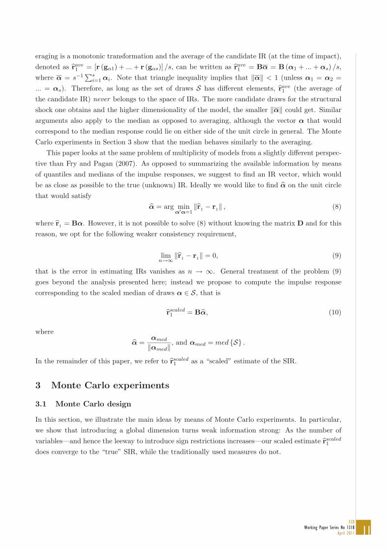
1 (the average ofthe candidate IR) never belongs to the space of IRs. The more candidate draws for the structuralshock one obtains and the higher dimensionality of the model, the smaller ‖α‖ could get. Similararguments also apply to the median as opposed to averaging, although the vector α that wouldcorrespond to the median response could lie on either side of the unit circle in general. The MonteCarlo experiments in Section 3 show that the median behaves similarly to the averaging.

This paper looks at the same problem of multiplicity of models from a slightly different perspec-tive than Fry and Pagan (2007). As opposed to summarizing the available information by meansof quantiles and medians of the impulse responses, we suggest to find an IR vector, which wouldbe as close as possible to the true (unknown) IR. Ideally we would like to find α on the unit circlethat would satisfy

α = arg minα′α=1

‖r1 − r1‖ , (8)

where r1 = Bα. However, it is not possible to solve (8) without knowing the matrix D and for thisreason, we opt for the following weaker consistency requirement,

limn→∞ ‖r1 − r1‖ = 0, (9)

that is the error in estimating IRs vanishes as n → ∞. General treatment of the problem (9)goes beyond the analysis presented here; instead we propose to compute the impulse responsecorresponding to the scaled median of draws α ∈ S, that is

rscaled1 = Bα, (10)

whereα =

αmed

‖αmed‖ , and αmed = med {S} .

In the remainder of this paper, we refer to rscaled1 as a “scaled” estimate of the SIR.

3 Monte Carlo experiments

3.1 Monte Carlo design

In this section, we illustrate the main ideas by means of Monte Carlo experiments. In particular,we show that introducing a global dimension turns weak information strong: As the number ofvariables—and hence the leeway to introduce sign restrictions increases—our scaled estimate rscaled

1

does converge to the “true” SIR, while the traditionally used measures do not.

12ECB


April 2011

8The decomposition of Σ is arbitrary and other decompositions should yield similar results since no other infor-mation, besides the signs of responses are imposed (see, for instance, Uhlig, 2005).

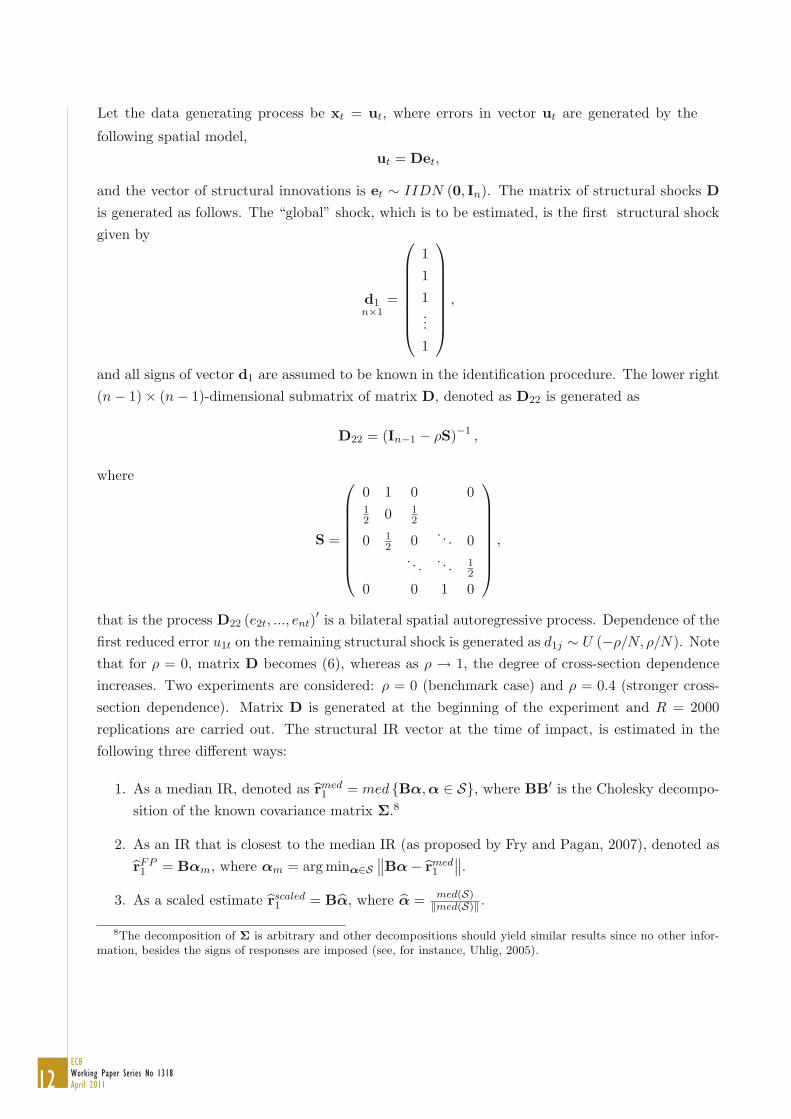
following spatial model,ut = Det,

and the vector of structural innovations is et ∼ IIDN (0, In). The matrix of structural shocks D

is generated as follows. The “global” shock, which is to be estimated, is the first structural shockgiven by

d1n×1

=

⎛⎜⎜⎜⎜⎜⎜⎜⎝

111...1

⎞⎟⎟⎟⎟⎟⎟⎟⎠

,

and all signs of vector d1 are assumed to be known in the identification procedure. The lower right(n − 1) × (n − 1)-dimensional submatrix of matrix D, denoted as D22 is generated as

D22 = (In−1 − ρS)−1 ,

where

S =

⎛⎜⎜⎜⎜⎜⎜⎜⎝

0 1 0 012 0 1

2

0 12 0

. . . 0. . . . . . 1

2

0 0 1 0

⎞⎟⎟⎟⎟⎟⎟⎟⎠

,

that is the process D22 (e2t, ..., ent)′ is a bilateral spatial autoregressive process. Dependence of the

first reduced error u1t on the remaining structural shock is generated as d1j ∼ U (−ρ/N, ρ/N). Notethat for ρ = 0, matrix D becomes (6), whereas as ρ → 1, the degree of cross-section dependenceincreases. Two experiments are considered: ρ = 0 (benchmark case) and ρ = 0.4 (stronger cross-section dependence). Matrix D is generated at the beginning of the experiment and R = 2000replications are carried out. The structural IR vector at the time of impact, is estimated in thefollowing three different ways:

1. As a median IR, denoted as rmed1 = med {Bα,α ∈ S}, where BB′ is the Cholesky decompo-

sition of the known covariance matrix Σ.8

2. As an IR that is closest to the median IR (as proposed by Fry and Pagan, 2007), denoted asrFP1 = Bαm, where αm = arg minα∈S

∥∥Bα − rmed1

∥∥.

3. As a scaled estimate rscaled1 = Bα, where α = med(S)

‖med(S)‖ .

Let the data generating process be xt = ut, where errors in vector ut are generated by the

13ECB


April 2011

the signs of d1. The vector α is generated randomly as

α =η

‖η‖ ,

where η ∼ N (0, In). The number of draws that satisfy the sign restrictions are chosen to bes ∈ {100, 500, 1000, 5000}.

3.2 Monte Carlo findings

In order to provide a first impression of the performance of the summary measures under inspec-tion, Figures 1–2 plot the histograms of the errors of the estimated structural vector r1 for 2000repetitions of the benchmark experiment (ρ = 0) and two choices for the dimension of the model,(n, s) ∈ {(5, 100) ; (20, 1000)}. Two different metrics for computing the error as the distance be-tween estimated SIRs and true SIRs are considered: the maximum absolute row sum norm, denotedas ‖r1 − r1‖r, and the euclidean norm, denoted as ‖r1 − r1‖.

As can be inferred from Figure 1, which plots the absolute frequency of the errors computedas euclidian norm, both the median impulse response as well as the measure suggested by Fry andPagan (2007) perform less well than the scaled response as proposed here.

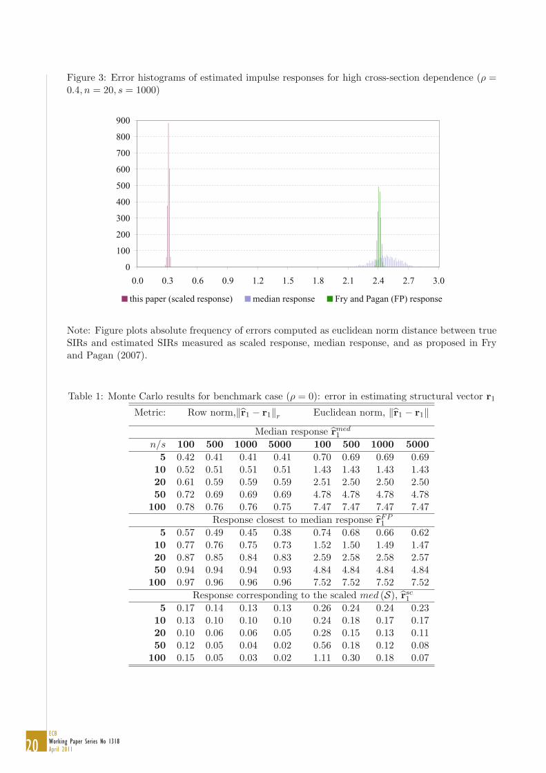
Furthermore, comparing the errors obtained in the relatively smaller system as shown in Figure1 with the errors obtained in a relatively larger system embedding more information on the truesigns of the IRs as shown in Figure 2 shows that the error in estimating the SIRs actually increasesin n and hence the number of restrictions imposed when using the conventional summary measures.The scaled response estimator rscaled

1 however improves with rising n, and hence fulfills the intuitiveconsistency property outlined in Section 1. The latter result is robust to the degree of cross-sectiondependence as evidenced by Figure 3.

The preliminary findings from inspection of the error histograms are confirmed when consid-ering a wide range of alternative values for the model dimension. Tables 1–2 report the aver-age error of the individual estimates of the structural impulse response vector d1 for (n, s) ∈{(5, 10, 20, 50, 100) ; (100, 500, 1000, 5000)} for both the benchmark experiment (ρ = 0) as well asthe case of higher cross-section dependence (ρ = 0.4). It can be inferred from Table 1 that themedian response (rmed

1 ) as well as the response which is closest to median response (rFP1 ) do not

provide a good estimate of the structural impulse response. First, performance does not improvein the number of models that satisfy sign restrictions. Second, the estimated responses becomeeven worse as the number of variables and hence the numbers of signs restrictions increases. Theseresults confirm that even if a large amount of sign restrictions is imposed, the conventional sum-mary measures rmed

1 and rFP1 can be highly misleading when interpreted as a “consensus” view.

In particular, both∥∥rFP

1 − r1

∥∥ and∥∥rmed

1 − r1

∥∥ seem to diverge to infinity with n and thereforethe estimation error is arbitrarily large for n large enough. On the other hand, the scaled responserscaled1 , clearly gets closer to the true response as n and the number of draws increase. Finally, the

results also show that introducing a “global dimension” helps gaining accuracy: for a system of

The covariance matrix Σ is taken to be known. Matrix D is treated as unknown, except for

14ECB


April 2011

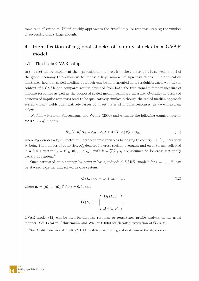
some tens of variables, rscaled1 quickly approaches the “true” impulse response keeping the number

of successful draws large enough.

4 Identification of a global shock: oil supply shocks in a GVAR

model

4.1 The basic GVAR setup

In this section, we implement the sign restriction approach in the context of a large scale model ofthe global economy that allows us to impose a large number of sign restrictions. The applicationillustrates how our scaled median approach can be implemented in a straightforward way in thecontext of a GVAR and compares results obtained from both the traditional summary measure ofimpulse responses as well as the proposed scaled median summary measure. Overall, the observedpatterns of impulse responses tend to be qualitatively similar, although the scaled median approachsystematically yields quantitatively larger point estimates of impulse responses, as we will explainbelow.

We follow Pesaran, Schuermann and Weiner (2004) and estimate the following country-specificVARX∗ (p, q) models:

Φii (L, pi)xit = ai0 + ai1t + Λi (L, qi)x∗it + uit, (11)

where xit denotes a ki×1 vector of macroeconomic variables belonging to country i ∈ {1, .., N} withN being the number of countries, x∗

it denotes its cross-section averages, and error terms, collectedin a k × 1 vector ut = (u′

1t,u′2t, ...,u

′Nt)

′ with k =∑N

i=1 ki are assumed to be cross-sectionallyweakly dependent.9

Once estimated on a country by country basis, individual VARX∗ models for i = 1, .., N , canbe stacked together and solved as one system:

G (L, p)xt = a0 + a1t + ut, (12)

where a� = (a′�1, ...,a

′�N )′ for � = 0, 1, and

G (L, p) =

⎛⎜⎜⎝

B1 (L, p)...

BN (L, p)

⎞⎟⎟⎠ .

GVAR model (12) can be used for impulse response or persistence profile analysis in the usualmanner. See Pesaran, Schuermann and Wiener (2004) for detailed exposition of GVARs.

9See Chudik, Pesaran and Tosetti (2011) for a definition of strong and weak cross section dependence.

15ECB


April 2011

4.2 Data and sign restrictions

We set pi = p = 2 and qi = q = 1 and estimate a GVAR in first differences with quarterly dataover the period 1979:Q3–2003Q3 for N = 26 countries.10 We include four country-specific variables—real output, inflation, a short-term interest rate, and the real exchange rate—as well as real oilprices as an observable global factor.

In order to identify oil supply shocks we rely on a simple identification scheme that allows usto discriminate oil supply shocks from a large set of alternative shocks. In particular, we requirenegative oil supply shocks to be contemporaneously associated with (i) a decrease in real outputacross all oil-importers and (ii) an increase in real oil prices. In all, we impose 21 contempora-neous sign restrictions. We do not impose any restrictions on real output in countries that havebeen significant oil-exporters over the sample period.11 To the extent that no other economicallymeaningful shocks are able to produce a negative correlation between real output and real oil pricesacross all oil-importing economies, this identification scheme uniquely identifies oil supply shocks.

4.3 Empirical results

In the following we analyse the effect of negative oil supply shocks on (i) real output in differentregions of the global economy including oil-exporting economies themselves; as well as (ii) on globalexchange rate configurations.

Figure 4 gives a general overview of the reaction of output to a one-standard deviation shock tooil supply. On average, mature economies—including the United States and the euro area—tendto record a decline in real output by between 0.5 and 0.75% cumulated over the four quartersfollowing a one-standard deviation oil supply shock (that causes oil prices to increase by 2.4%).Emerging economies—both in Latin America and Asia—record somewhat higher declines in growthof on average between 1 and 1.5%. The stronger effect on emerging economies could be a reflectionof higher energy intensity of production in these countries, on the one hand, and dependenceon external demand from mature economies, on the other hand. In this respect, China standsout as a notable exception with a relatively modest reaction of output to the oil supply shock,possibly reflecting the fact that despite high energy intensity a large part of energy demand is metdomestically. Interestingly though not largely unexpectedly, real output also declines across alloil-exporting economies in our sample, including Saudi Arabia and Norway, although to a lesserextent, despite the reaction of real output being unrestricted in the identification procedure.

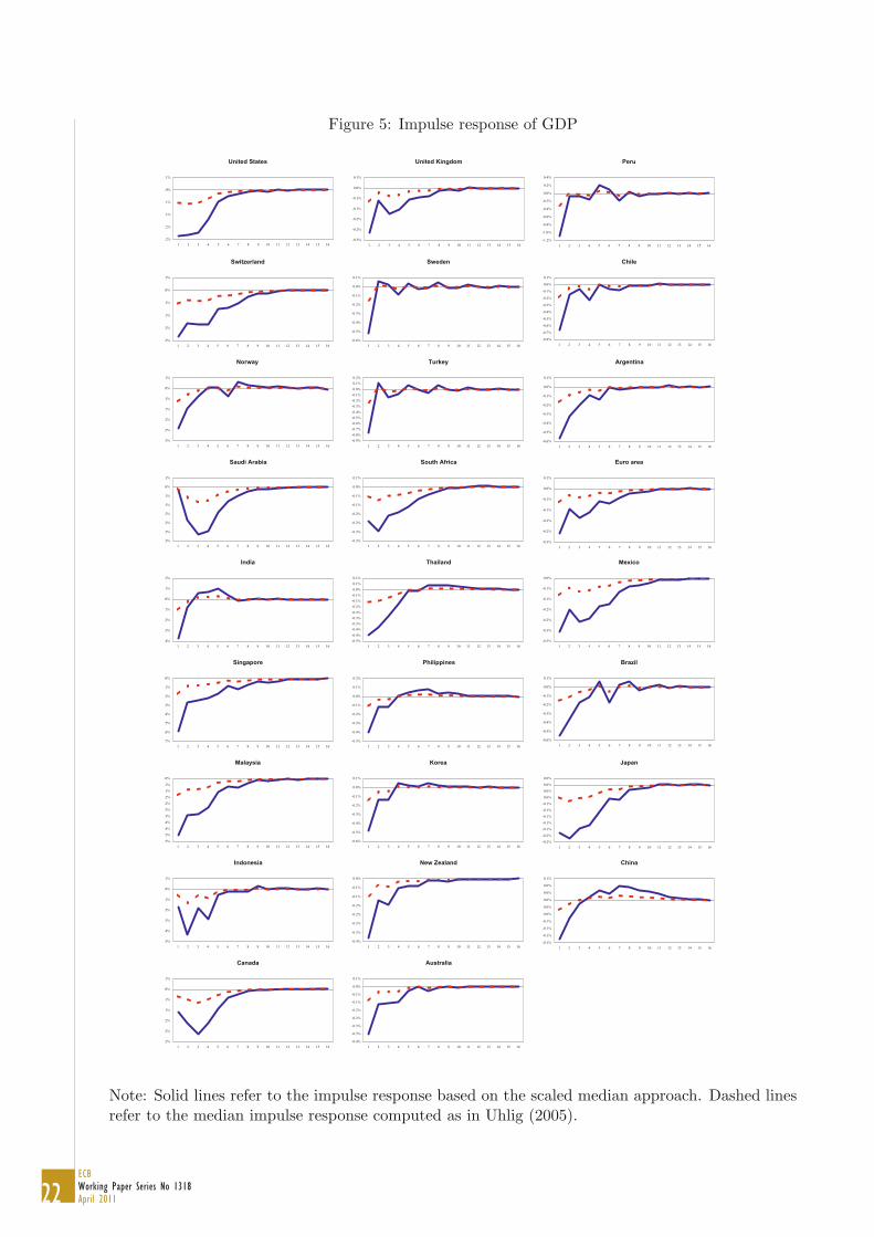
Figure 5 provides further detail and compares the impulse response based on the scaled medianapproach to impulse responses computed as in Uhlig (2005). A main finding from this exerciseis that—while the patterns of impulse responses are qualitatively comparable—our scaled medianimpulse response tends to systemically yield larger point estimates of the shocks under inspection.

10The sample includes Argentina, Australia, Brazil, Canada, Chile, China, Euro area, India, Indonesia, Japan,Korea, Malaysia, Mexico, New Zealand, Norway, Peru, Philippines, Saudi Arabia, Singapore, South Africa, Sweden,Switzerland, Thailand, Turkey, United Kingdom, United states.

11We take these countries to be Saudi Arabia, Norway, Indonesia, Mexico and the United Kingdom.

16ECB


April 2011

The quantitative difference is sizeable as impulse responses based on the scaled median tend to beabout 3 times larger than those based on the traditional measure. This is because the traditionalmeasure is based on median values of α that—at least in the case of a single shock—is bound tolie within the unit circle (and therefore does not belong to the space of impulse responses), whileour scaling approach avoids this caveat (and rscaled

1 belongs to the space of IRs).Finally, results for the real exchange rate are summarised in Figures 6 and 7. As expected,

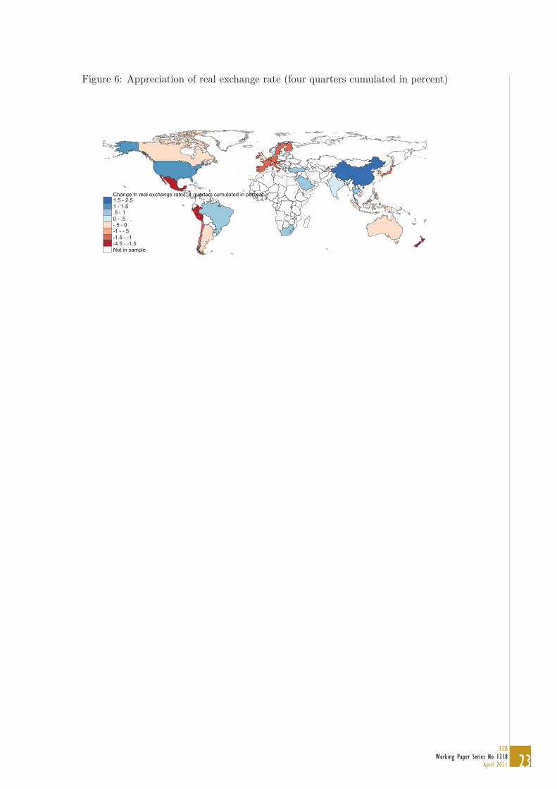
oil-importers’ real exchange rates mostly tend to depreciate in response to the negative terms oftrade shock by on average between 0.5 and 1.5%, whereas the large oil exporters’ appreciate byup to 1%. Maybe surprisingly, the United States appreciates by 1.3%. One rationalisation for thisunexpected result could be recycling of oil-exporters’ increased revenues in US financial markets.As a final note, Figure 7 shows that as in the case of real output before, our measure yields similarbut systematically larger point estimates of impulse responses confirming our findings above.

5 Identification in a small scale model: US monetary policy shocks

In the following, this section assess how our alternative summary measure of impulse responsescompares to the traditionally used median impulse response measure in the context of a small scalesingle country model.

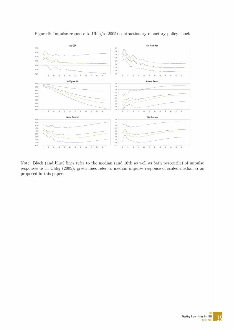
In order to allow for a meaningful comparison, we use as a benchmark the application presentedin Uhlig (2005), which employs sign restrictions to identify the effects of a contractionary monetarypolicy shock. In particular, we compute impulse responses to a contractionary monetary shockidentified via the same sign restrictions as in Uhlig (2005) using both the traditional median impulseresponse and the approach based on scaled median draws from the unit circle, as proposed in thispaper.

We use the data and code provided by Uhlig (2005) with monthly data (partly generated frominterpolation) for the period 1965:01–2003:12 on real GDP, GDP deflator, commodity prices, federalfunds rate, non-borrowed reserves, and total reserves. Following Uhlig (2005), we estimate a VAR inlevels using 12 lags. Contractionary monetary policy is identified via sign restrictions implementedas follows. The GDP deflator, the commodity price index and non-borrowed reserves are restrictednot to be positive and the federal funds rate is restricted not to be negative for k = 5 months afterthe shock. We take 1,000 draws from the posterior for each of which we compute 40,000 drawsfrom the unit circle. 12

12Uhligs code is based on 200 draws from each the posterior and the unit circle, resulting in overall 40,000 draws,but stops after having generated 1,000 draws that satisfy the sign restrictions. From these 1,000 draws impulseresponses are generated and summarised in terms of their median. In order to compute the alternative summarymeasure proposed in this paper, we need to compute the median of draws of α (for which the corresponding impulseresponses satisfy the sign restrictions) for each draw from the posterior. Hence, an overall larger amount of drawsfrom both the posterior and the unit circle is need in order to compute meaningful medians at both stages. Wetherefore increase the number of draws from the posterior to 1,000 draws for each of which we compute 40,000 drawsfrom the unit circle. This leaves us with on average around 1,100 (and in no case fewer than 1,000) accepted drawsfrom the unit circle for each of the 1,000 draws from the posterior distribution. From these roughly 1,100 draws wecompute the scaled median and corresponding impulse responses, for which we then report the median across all1,000 draws from the posterior.

17ECB


April 2011

Impulse responses are presented in Figure 8. First, we note that the code exactly replicatesthe impulse responses depicted in Uhlig (2005). Secondly, as in the case of the large scale modelpresented before, impulse responses are qualitatively not very different. However, impulse responsesbased on the scaled median α also in the small model tend to be quantitatively larger, by betweenone quarter and one half, confirming the findings from the previous analysis.

6 Concluding remarks

Identification of structural VARs by means of sign restrictions has become increasingly popular inapplied econometrics over the recent past. Maybe surprisingly, the performance of identificationschemes using sign restriction has only received limited attention and there is indeed little evidencethat imposing sign restrictions actually helps identifying structural shocks at all. Sign restrictionsdo not pin down a unique structural model and it is therefore not surprising that any sign restric-tion identification procedure is bound to be imperfect. Nevertheless, one would expect that withan increasing number of sign restrictions imposed one should obtain a better understanding of thestructural shock in question. The global or cross-section dimension offers an intuitive and straight-forward way of imposing a large number of sign restrictions to identify shocks that are global innature—i.e. shocks that affect many cross-section units at the same time.

The mainstream literature reports the median of the impulse responses, which is sometimesinterpreted as a “consensus” view of the magnitudes of the responses, and quantiles are used togive an impression of the distribution of impulse responses. The global dimension offers a new wayof dealing with the problem of summarising information. We look at the summary measure as anestimation problem and expect that with an increasing cross-section dimension and an increasingnumber of restrictions imposed, the summary measures gets closer to the true structural impulseresponse (consistency property). This allows us to label the summary measure as our “best guess”whereas it is difficult to interpret the traditionally reported median impulse response. Indeed, themedian impulse response does not get closer to the structural IR with an increasing number ofrestrictions imposed. We propose an alternative way of summarising information and show bymeans of Monte Carlo simulations that it seems to satisfy the intuitive consistency property and itoutperforms the traditional summary measures.

Finally we implement the sign restriction approach in the context of a Global VAR (GVAR)model of the world economy, which given its global dimension allows for imposing a large numberof sign restrictions, and we identify the effect of oil shocks on the global economy. Our resultssuggest that negative oil supply shocks (i) have a stronger impact on emerging economies’ realoutput as compared to mature economies, (ii) have a negative impact on real growth in oil-exportingeconomies as well, (iii) tend to cause an appreciation (depreciation) of oil-exporters’ (oil-importers’)real exchange rates but also lead to an appreciation of the US dollar. One possible explanationwould be recycling of oil-exporters’ increased revenues in US financial markets.

18ECB


April 2011

References

Bernanke, Ben S., 1986, Alternative Explanations of the Money-Income Correlation. Carnegie-RochesterConference Series on Public Policy, Elsevier, 25(1), pp. 49-99.

Blanchard, Olivier J. and Mark W. Watson, 1986, ”Are Business Cycles All Alike?,” NBER Chapters,in: The American Business Cycle: Continuity and Change, pages 123-180 National Bureau of EconomicResearch.

Canova, Fabio and Gianni de Nicolo, 2002, Monetary Disturbances Matter for Business Fluctuations in theG-7. Journal of Monetary Economics, 49, pp. 1131–1159

Canova, Fabio and Joaquim Pina, 1999, Monetary Policy Misspecification in VAR Models. Centre forEconomic Policy Research, Discussion Paper No 2333.

Faust, Jon, 1998, The Robustness of Identified VAR Conclusions About Money. Carnegie-Rochester Con-ference Series in Public Policy, 49(1), pp. 207–244.

Fry, Renee and Adrian Pagan, 2007, Some Issues in Using Sign Restrictions for Identifying Structural VARs.National Centre for Econometric Research, Working Paper No. 14, April 2007.

Mountford, Andrew and Harald Uhlig, 2009, What are the Effects of Fiscal Policy Shocks? Journal ofApplied Econometrics, 24(6), pp. 960–992.

Paustian, Matthias, 2007, Assessing sign restrictions. The B.E. Journal of Macroeconomics (Topics), 7(1),Article 23.

Chudik, Alexander, Pesaran, M. Hashem and Elisa Tosetti, 2011, Weak and Strong Cross Section Depen-dence and Estimation of Large Panels, forthcomming in the Econometrics Journal.

Pesaran, M. H., Til Schuermann and Scott M. Weiner, 2004, Modelling Regional Interdependencies UsingA Global Error-Correcting Macroeconometric Model, Journal of Business and Economics Statistics, Vol.:22(2), pp.: 129-162

Rubio-Ramirez, Juan, Waggoner, Daniel and Tao Zha, 2006, Markov-Switching Structural Vector Autore-gressions: Theory and Application. Computing in Economics and Finance 2006, 69, Society for Computa-tional Economics.

Uhlig, Harald, 2005, What are the Effects of Monetary Policy on Output? Results from an AgnosticIdentification Procedure. Journal of Monetary Economics, 52, pp. 381–419.

19ECB


April 2011

Figure 1: Error histograms of estimated impulse responses for small benchmark model (ρ = 0, n =5, s = 100)

0

20

40

60

80

100

120

140

160

180

200

0.0 0.1 0.2 0.3 0.4 0.5 0.6 0.7 0.8 0.9 1.0

this paper (scaled response) median response Fry and Pagan (FP) response

Note: Figure plots absolute frequency of errors computed as euclidean norm distance between trueSIRs and estimated SIRs measured as scaled response, median response, and as proposed in Fryand Pagan (2007).

Figure 2: Error histograms of estimated impulse responses for large benchmark model (ρ = 0, n =20, s = 1000)

0

100

200

300

400

500

600

700

800

900

0.0 0.3 0.5 0.8 1.0 1.3 1.5 1.8 2.0 2.3 2.5 2.8 3.0



20ECB


April 2011

Figure 3: Error histograms of estimated impulse responses for high cross-section dependence (ρ =0.4, n = 20, s = 1000)

0

100

200

300

400

500

600

700

800

900

0.0 0.3 0.6 0.9 1.2 1.5 1.8 2.1 2.4 2.7 3.0



Table 1: Monte Carlo results for benchmark case (ρ = 0): error in estimating structural vector r1

Metric: Row norm,‖r1 − r1‖r Euclidean norm, ‖r1 − r1‖Median response rmed

1

n/s 100 500 1000 5000 100 500 1000 50005 0.42 0.41 0.41 0.41 0.70 0.69 0.69 0.69

10 0.52 0.51 0.51 0.51 1.43 1.43 1.43 1.4320 0.61 0.59 0.59 0.59 2.51 2.50 2.50 2.5050 0.72 0.69 0.69 0.69 4.78 4.78 4.78 4.78

100 0.78 0.76 0.76 0.75 7.47 7.47 7.47 7.47Response closest to median response rFP

1

5 0.57 0.49 0.45 0.38 0.74 0.68 0.66 0.6210 0.77 0.76 0.75 0.73 1.52 1.50 1.49 1.4720 0.87 0.85 0.84 0.83 2.59 2.58 2.58 2.5750 0.94 0.94 0.94 0.93 4.84 4.84 4.84 4.84

100 0.97 0.96 0.96 0.96 7.52 7.52 7.52 7.52Response corresponding to the scaled med (S), rsc

1

5 0.17 0.14 0.13 0.13 0.26 0.24 0.24 0.2310 0.13 0.10 0.10 0.10 0.24 0.18 0.17 0.1720 0.10 0.06 0.06 0.05 0.28 0.15 0.13 0.1150 0.12 0.05 0.04 0.02 0.56 0.18 0.12 0.08

100 0.15 0.05 0.03 0.02 1.11 0.30 0.18 0.07

21ECB


April 2011

Table 2: Monte Carlo results for high cross-section dependence (ρ = 0.4): error in estimatingstructural vector r1

Metric: Row norm,‖r1 − r1‖r Euclidean norm, ‖r1 − r1‖Median response rmed

1

n/s 100 500 1000 5000 100 500 1000 50005 0.49 0.49 0.49 0.49 0.62 0.62 0.61 0.61

10 0.56 0.56 0.56 0.56 1.34 1.34 1.34 1.3420 0.61 0.60 0.60 0.60 2.41 2.40 2.40 2.4050 0.70 0.68 0.68 0.68 4.64 4.64 4.64 4.64

100 0.76 0.74 0.74 0.74 7.29 7.29 7.29 7.29Response closest to median response rFP

1

5 0.48 0.40 0.38 0.35 0.64 0.55 0.52 0.4910 0.76 0.74 0.73 0.69 1.43 1.39 1.38 1.3520 0.86 0.85 0.84 0.84 2.50 2.48 2.48 2.4750 0.93 0.93 0.92 0.92 4.72 4.71 4.70 4.70

100 0.96 0.96 0.96 0.95 7.35 7.35 7.35 7.34Response corresponding to the scaled med (S), rsc

1

5 0.33 0.31 0.31 0.30 0.56 0.57 0.57 0.5710 0.22 0.19 0.18 0.17 0.44 0.44 0.44 0.4420 0.15 0.12 0.11 0.11 0.34 0.31 0.31 0.3150 0.11 0.06 0.06 0.04 0.47 0.21 0.19 0.19

100 0.14 0.05 0.04 0.03 0.94 0.25 0.17 0.13

Figure 4: Output decline in response to one standard-deviation negative oil supply shock (fourquarters cumulated in percent)

Real output reduction, 4 quarters cumulated in percent1 - 1.5.75 - 1.5 - .75.25 - .50 - .25Not in sample

22ECB


April 2011

Figure 5: Impulse response of GDP

United States United Kingdom Peru

Switzerland Sweden Chile

Norway Turkey Argentina

Saudi Arabia South Africa Euro area

India Thailand Mexico

Singapore Philippines Brazil

Malaysia Korea Japan

Indonesia New Zealand China

Canada Australia

.2%

.2%

.1%

.1%

.0%

.1%

1 2 3 4 5 6 7 8 9 10 11 12 13 14 15 16

-0.3%

-0.2%

-0.2%

-0.1%

-0.1%

0.0%

0.1%

1 2 3 4 5 6 7 8 9 10 11 12 13 14 15 16

.2%

.2%

.1%

.1%

.0%

.1%

1 2 3 4 5 6 7 8 9 10 11 12 13 14 15 16

-0.6%

-0.5%

-0.4%

-0.3%

-0.2%

-0.1%

0.0%

0.1%

1 2 3 4 5 6 7 8 9 10 11 12 13 14 15 16

.3%

.2%

.2%

.1%

.1%

.0%

.1%

1 2 3 4 5 6 7 8 9 10 11 12 13 14 15 16

-0.9%

-0.8%

-0.7%

-0.6%

-0.5%

-0.4%

-0.3%

-0.2%

-0.1%

0.0%

0.1%

0.2%

1 2 3 4 5 6 7 8 9 10 11 12 13 14 15 16

.3%

.3%

.2%

.2%

.1%

.1%

.0%

.1%

1 2 3 4 5 6 7 8 9 10 11 12 13 14 15 16

-0.3%

-0.3%

-0.2%

-0.2%

-0.1%

-0.1%

0.0%

0.1%

1 2 3 4 5 6 7 8 9 10 11 12 13 14 15 16

.4%

.3%

.2%

.1%

.0%

.1%

.2%

1 2 3 4 5 6 7 8 9 10 11 12 13 14 15 16

-0.5%

-0.4%

-0.4%

-0.3%

-0.3%

-0.2%

-0.2%

-0.1%

-0.1%

0.0%

0.1%

0.1%

1 2 3 4 5 6 7 8 9 10 11 12 13 14 15 16

.7%

.6%

.5%

.4%

.3%

.2%

.1%

.0%

1 2 3 4 5 6 7 8 9 10 11 12 13 14 15 16

-0.5%

-0.4%

-0.3%

-0.2%

-0.1%

0.0%

0.1%

0.2%

1 2 3 4 5 6 7 8 9 10 11 12 13 14 15 16

.5%

.5%

.4%

.4%

.3%

.3%

.2%

.2%

.1%

.1%

.0%

1 2 3 4 5 6 7 8 9 10 11 12 13 14 15 16

-0.6%

-0.5%

-0.4%

-0.3%

-0.2%

-0.1%

0.0%

0.1%

1 2 3 4 5 6 7 8 9 10 11 12 13 14 15 16

.5%

.4%

.3%

.2%

.1%

.0%

.1%

1 2 3 4 5 6 7 8 9 10 11 12 13 14 15 16

-0.4%

-0.3%

-0.3%

-0.2%

-0.2%

-0.1%

-0.1%

0.0%

1 2 3 4 5 6 7 8 9 10 11 12 13 14 15 16

.3%

.2%

.2%

.1%

.1%

.0%

.1%

1 2 3 4 5 6 7 8 9 10 11 12 13 14 15 16

-0.4%

-0.3%

-0.3%

-0.2%

-0.2%

-0.1%

-0.1%

0.0%

0.1%

1 2 3 4 5 6 7 8 9 10 11 12 13 14 15 16

-1.2%

-1.0%

-0.8%

-0.6%

-0.4%

-0.2%

0.0%

0.2%

0.4%

1 2 3 4 5 6 7 8 9 10 11 12 13 14 15 16

-0.3%

-0.3%

-0.2%

-0.2%

-0.1%

-0.1%

0.0%

1 2 3 4 5 6 7 8 9 10 11 12 13 14 15 16

-0.8%

-0.7%

-0.6%

-0.5%

-0.4%

-0.3%

-0.2%

-0.1%

0.0%

0.1%

1 2 3 4 5 6 7 8 9 10 11 12 13 14 15 16

-0.6%

-0.5%

-0.4%

-0.3%

-0.2%

-0.1%

0.0%

0.1%

1 2 3 4 5 6 7 8 9 10 11 12 13 14 15 16

-0.6%

-0.5%

-0.4%

-0.3%

-0.2%

-0.1%

0.0%

0.1%

1 2 3 4 5 6 7 8 9 10 11 12 13 14 15 16

-0.2%

-0.2%

-0.1%

-0.1%

-0.1%

-0.1%

-0.1%

0.0%

0.0%

0.0%

0.0%

1 2 3 4 5 6 7 8 9 10 11 12 13 14 15 16

-0.3%

-0.2%

-0.2%

-0.1%

-0.1%

0.0%

0.1%

1 2 3 4 5 6 7 8 9 10 11 12 13 14 15 16

-0.1%

-0.1%

-0.1%

-0.1%

0.0%

0.0%

0.0%

0.0%

0.0%

0.1%

1 2 3 4 5 6 7 8 9 10 11 12 13 14 15 16

Note: Solid lines refer to the impulse response based on the scaled median approach. Dashed linesrefer to the median impulse response computed as in Uhlig (2005).

23ECB


April 2011

Figure 6: Appreciation of real exchange rate (four quarters cumulated in percent)

Change in real exchange rates, 4 quarters cumulated in percent1.5 - 2.51 - 1.5.5 - 10 - .5-.5 - 0-1 - -.5-1.5 - -1-4.5 - -1.5Not in sample

24ECB


April 2011

Figure 7: Impulse response of real effective exchange rates

United States United Kingdom Peru

Switzerland Sweden Chile

Norway Turkey Argentina

Saudi Arabia South Africa Euro area

India Thailand Mexico

Singapore Philippines Brazil

Malaysia Korea Japan

Indonesia New Zealand China

Canada Australia

.2%

.2%

.1%

.1%

.0%

.1%

1 2 3 4 5 6 7 8 9 10 11 12 13 14 15 16

-0.3%

-0.2%

-0.2%

-0.1%

-0.1%

0.0%

0.1%

1 2 3 4 5 6 7 8 9 10 11 12 13 14 15 16

.2%

.2%

.1%

.1%

.0%

.1%

1 2 3 4 5 6 7 8 9 10 11 12 13 14 15 16

-0.6%

-0.5%

-0.4%

-0.3%

-0.2%

-0.1%

0.0%

0.1%

1 2 3 4 5 6 7 8 9 10 11 12 13 14 15 16

.3%

.2%

.2%

.1%

.1%

.0%

.1%

1 2 3 4 5 6 7 8 9 10 11 12 13 14 15 16

-0.9%

-0.8%

-0.7%

-0.6%

-0.5%

-0.4%

-0.3%

-0.2%

-0.1%

0.0%

0.1%

0.2%

1 2 3 4 5 6 7 8 9 10 11 12 13 14 15 16

.3%

.3%

.2%

.2%

.1%

.1%

.0%

.1%

1 2 3 4 5 6 7 8 9 10 11 12 13 14 15 16

-0.3%

-0.3%

-0.2%

-0.2%

-0.1%

-0.1%

0.0%

0.1%

1 2 3 4 5 6 7 8 9 10 11 12 13 14 15 16

.4%

.3%

.2%

.1%

.0%

.1%

.2%

1 2 3 4 5 6 7 8 9 10 11 12 13 14 15 16

-0.5%

-0.4%

-0.4%

-0.3%

-0.3%

-0.2%

-0.2%

-0.1%

-0.1%

0.0%

0.1%

0.1%

1 2 3 4 5 6 7 8 9 10 11 12 13 14 15 16

.7%

.6%

.5%

.4%

.3%

.2%

.1%

.0%

1 2 3 4 5 6 7 8 9 10 11 12 13 14 15 16

-0.5%

-0.4%

-0.3%

-0.2%

-0.1%

0.0%

0.1%

0.2%

1 2 3 4 5 6 7 8 9 10 11 12 13 14 15 16

.5%

.5%

.4%

.4%

.3%

.3%

.2%

.2%

.1%

.1%

.0%

1 2 3 4 5 6 7 8 9 10 11 12 13 14 15 16

-0.6%

-0.5%

-0.4%

-0.3%

-0.2%

-0.1%

0.0%

0.1%

1 2 3 4 5 6 7 8 9 10 11 12 13 14 15 16

.5%

.4%

.3%

.2%

.1%

.0%

.1%

1 2 3 4 5 6 7 8 9 10 11 12 13 14 15 16

-0.4%

-0.3%

-0.3%

-0.2%

-0.2%

-0.1%

-0.1%

0.0%

1 2 3 4 5 6 7 8 9 10 11 12 13 14 15 16

.3%

.2%

.2%

.1%

.1%

.0%

.1%

1 2 3 4 5 6 7 8 9 10 11 12 13 14 15 16

-0.4%

-0.3%

-0.3%

-0.2%

-0.2%

-0.1%

-0.1%

0.0%

0.1%

1 2 3 4 5 6 7 8 9 10 11 12 13 14 15 16

-1.2%

-1.0%

-0.8%

-0.6%

-0.4%

-0.2%

0.0%

0.2%

0.4%

1 2 3 4 5 6 7 8 9 10 11 12 13 14 15 16

-0.3%

-0.3%

-0.2%

-0.2%

-0.1%

-0.1%

0.0%

1 2 3 4 5 6 7 8 9 10 11 12 13 14 15 16

-0.8%

-0.7%

-0.6%

-0.5%

-0.4%

-0.3%

-0.2%

-0.1%

0.0%

0.1%

1 2 3 4 5 6 7 8 9 10 11 12 13 14 15 16

-0.6%

-0.5%

-0.4%

-0.3%

-0.2%

-0.1%

0.0%

0.1%

1 2 3 4 5 6 7 8 9 10 11 12 13 14 15 16

-0.6%

-0.5%

-0.4%

-0.3%

-0.2%

-0.1%

0.0%

0.1%

1 2 3 4 5 6 7 8 9 10 11 12 13 14 15 16

-0.2%

-0.2%

-0.1%

-0.1%

-0.1%

-0.1%

-0.1%

0.0%

0.0%

0.0%

0.0%

1 2 3 4 5 6 7 8 9 10 11 12 13 14 15 16

-0.3%

-0.2%

-0.2%

-0.1%

-0.1%

0.0%

0.1%

1 2 3 4 5 6 7 8 9 10 11 12 13 14 15 16

-0.1%

-0.1%

-0.1%

-0.1%

0.0%

0.0%

0.0%

0.0%

0.0%

0.1%

1 2 3 4 5 6 7 8 9 10 11 12 13 14 15 16

.1%

.0%

.1%

.2%

.3%

.4%

.5%

.6%

1 2 3 4 5 6 7 8 9 10 11 12 13 14 15 16

-0.3%

-0.2%

-0.1%

0.0%

0.1%

0.2%

0.3%

1 2 3 4 5 6 7 8 9 10 11 12 13 14 15 16

.4%

.3%

.3%

.2%

.2%

.1%

.1%

.0%

.1%

.1%

.2%

1 2 3 4 5 6 7 8 9 10 11 12 13 14 15 16

-0.6%

-0.5%

-0.4%

-0.3%

-0.2%

-0.1%

0.0%

0.1%

1 2 3 4 5 6 7 8 9 10 11 12 13 14 15 16

.1%

.1%

.0%

.1%

.1%

.2%

.2%

.3%

1 2 3 4 5 6 7 8 9 10 11 12 13 14 15 16

-0.8%

-0.6%

-0.4%

-0.2%

0.0%

0.2%

0.4%

0.6%

0.8%

1 2 3 4 5 6 7 8 9 10 11 12 13 14 15 16

0%

1%

1%

2%

2%

3%

3%

4%

4%

5%

1 2 3 4 5 6 7 8 9 10 11 12 13 14 15 16

-0.1%

-0.1%

0.0%

0.1%

0.1%

0.2%

0.2%

0.3%

0.3%

0.4%

0.4%

1 2 3 4 5 6 7 8 9 10 11 12 13 14 15 16

.4%

.3%

.2%

.1%

.0%

.1%

.2%

.3%

.4%

.5%

.6%

1 2 3 4 5 6 7 8 9 10 11 12 13 14 15 16

-0.8%

-0.6%

-0.4%

-0.2%

0.0%

0.2%

0.4%

0.6%

0.8%

1 2 3 4 5 6 7 8 9 10 11 12 13 14 15 16

.3%

.2%

.2%

.1%

.1%

.0%

.1%

1 2 3 4 5 6 7 8 9 10 11 12 13 14 15 16

-1.4%

-1.2%

-1.0%

-0.8%

-0.6%

-0.4%

-0.2%

0.0%

0.2%

0.4%

0.6%

1 2 3 4 5 6 7 8 9 10 11 12 13 14 15 16

.1%

.1%

.0%

.1%

.1%

.2%

.2%

.3%

.3%

1 2 3 4 5 6 7 8 9 10 11 12 13 14 15 16

-1.0%

-0.8%

-0.6%

-0.4%

-0.2%

0.0%

0.2%

0.4%

1 2 3 4 5 6 7 8 9 10 11 12 13 14 15 16

.0%

.5%

.0%

.5%

.0%

.5%

.0%

1 2 3 4 5 6 7 8 9 10 11 12 13 14 15 16

-1.0%

-0.8%

-0.6%

-0.4%

-0.2%

0.0%

0.2%

1 2 3 4 5 6 7 8 9 10 11 12 13 14 15 16

.1%

.1%

.1%

.1%

.0%

.0%

.0%

.0%

.0%

.1%

.1%

1 2 3 4 5 6 7 8 9 10 11 12 13 14 15 16

-0.6%

-0.5%

-0.4%

-0.3%

-0.2%

-0.1%

0.0%

0.1%

0.2%

0.3%

1 2 3 4 5 6 7 8 9 10 11 12 13 14 15 16

-2.0%

-1.5%

-1.0%

-0.5%

0.0%

0.5%

1.0%

1 2 3 4 5 6 7 8 9 10 11 12 13 14 15 16

-1.4%

-1.2%

-1.0%

-0.8%

-0.6%

-0.4%

-0.2%

0.0%

0.2%

1 2 3 4 5 6 7 8 9 10 11 12 13 14 15 16

-1.2%

-1.0%

-0.8%

-0.6%

-0.4%

-0.2%

0.0%

0.2%

0.4%

1 2 3 4 5 6 7 8 9 10 11 12 13 14 15 16

-1.5%

-1.0%

-0.5%

0.0%

0.5%

1.0%

1.5%

1 2 3 4 5 6 7 8 9 10 11 12 13 14 15 16

-4.0%

-3.0%

-2.0%

-1.0%

0.0%

1.0%

2.0%

3.0%

4.0%

5.0%

6.0%

1 2 3 4 5 6 7 8 9 10 11 12 13 14 15 16

-0.8%

-0.6%

-0.4%

-0.2%

0.0%

0.2%

0.4%

1 2 3 4 5 6 7 8 9 10 11 12 13 14 15 16

-0.7%

-0.6%

-0.5%

-0.4%

-0.3%

-0.2%

-0.1%

0.0%

1 2 3 4 5 6 7 8 9 10 11 12 13 14 15 16

-0.4%

-0.2%

0.0%

0.2%

0.4%

0.6%

0.8%

1.0%

1.2%

1 2 3 4 5 6 7 8 9 10 11 12 13 14 15 16

Note: Solid lines refer to the impulse response based on the scaled median approach. Dashed linesrefer to the median impulse response computed as in Uhlig (2005).

25ECB


April 2011

Figure 8: Impulse response to Uhlig’s (2005) contractionary monetary policy shock

real GDP

0 5 10 15 20 25 30 35 40 45 50 55-0.20

-0.10

0.00

0.10

0.20

0.30

0.40

GDP price defl

0 5 10 15 20 25 30 35 40 45 50 55-0.80

-0.70

-0.60

-0.50

-0.40

-0.30

-0.20

-0.10

-0.00

Comm. Price Ind.

0 5 10 15 20 25 30 35 40 45 50 55-4.00

-3.50

-3.00

-2.50

-2.00

-1.50

-1.00

-0.50

0.00

0.50

Fed Funds Rate

0 5 10 15 20 25 30 35 40 45 50 55-0.30

-0.20

-0.10

0.00

0.10

0.20

0.30

0.40

0.50

Nonborr. Reserv .

0 5 10 15 20 25 30 35 40 45 50 55-1.75

-1.50

-1.25

-1.00

-0.75

-0.50

-0.25

0.00

0.25

0.50

Total Reserv es

0 5 10 15 20 25 30 35 40 45 50 55-1.75

-1.50

-1.25

-1.00

-0.75

-0.50

-0.25

0.00

0.25

0.50

Note: Black (and blue) lines refer to the median (and 16th as well as 84th percentile) of impulseresponses as in Uhlig (2005); green lines refer to median impulse response of scaled median α asproposed in this paper.

WORK ING PAPER SER I E SNO 1313 / MARCH 2011

by Cristian Badarinzaand Emil Margaritov

NEWS AND POLICY FORESIGHT IN A MACRO-FINANCE MODEL OF THE US

WORKING PAPER SERIES - European Central Bank PAPER SERIES NO 1318 / APRIL 2011 USING THE GLOBAL...

Documents

Transcript of WORKING PAPER SERIES - European Central Bank PAPER SERIES NO 1318 / APRIL 2011 USING THE GLOBAL...