Working Paper Series - European Central Bank · Working Paper Series The exchange rate, asymmetric...

Working Paper Series The exchange rate, asymmetric shocks and asymmetric distributions

Calin-Vlad Demian and Filippo di Mauro

No 1801 / June 2015

Note: This Working Paper should not be reported as representing the views of the European Central Bank (ECB). The views expressed are those of the authors and do not necessarily reflect those of the ECB

The Exchange rate, asymmetric shocks and asymmetric distributions

Calin-Vlad Demian and Filippo di Mauro

Abstract

The elasticity of exports to exchange rate fluctuations has been the subject of a large

literature without a clear consensus emerging. Using a novel sector-level dataset based

on firm level information, we show that exchange rate elasticities double in size when

the country and sector specific firm productivity distribution is taken into account in

empirical estimates. In addition, exports appear to be sensitive to appreciation episodes,

but rather unaffected by depreciations. Finally, only rather large changes in the exchange

rate appear to matter.

JEL codes: F14, F41, F31

Keywords: exchange rate elasticity, bilateral trade, productivity dispersion, TFP

ECB Working Paper 1801, June 2015 1

Non-technical Summary

The link between exchange rates and international trade has been the subject of a broad body of literature

without a clear consensus on the size of the effect emerging. Overall, there is a disconnect between

estimates using aggregate data and the ones using firm level information: macro estimates tend to be

insignificant or very close to zero while micro based research tends to find significant and economically

meaningful results. This paper attempts to bridge the gap between these two strands of the literature by

using sector level productivity statistics derived from firm level data as additional explanatory variables for

exports performance.

The main value added of the paper is empirical and derives from the use of a novel data set of productivity

statistics for 22 sectors in 10 European Union (EU) countries over 11 years, constructed from firm level

data, as part of the CompNet project at the ECB (Lopez-Garcia, di Mauro et al. 2015).

Four main results emerge from our estimations:

1. The inclusion of the productivity distribution in the export equation drastically affects the average

elasticity estimate by reducing unobserved bias. In our benchmark specification, it more than doubles

the estimated elasticity from 34% to 77%. Having derived sector specific elasticities allows us also to

compute country and EU-wide sector specific elasticities that are reliably identified.

2. In line with previous literature, the exchange rate elasticity of exports is lower in sectors where the

dispersion of firm productivity is higher.

3. Exports appear to react mostly to appreciations rather than depreciations. More specifically, in our

preferred specification, the exchange rate elasticity is about 80% in the case of appreciation and

statistically not significant in the case of depreciation. Moreover, the size of the coefficient in case of

appreciation is much larger than the baseline estimate, indicating that most of the empirically

estimated elasticity results from firms’ response to appreciation. The negative relationship between a

sector’s productivity dispersion and export elasticity still holds, but it is significant only in the case of

appreciation.

4. Exchange rate movements matters more when they are relatively sizeable. To show this, we split the

sample in relation to the size of the exchange rate change – i.e. outer 20% and 10- 90% range of the

distribution, respectively. Results show that in the case of small movements – which in our sample are

those between 9% depreciation and 12% appreciation – the exchange rate elasticity is smaller than for

extreme movements.


1. Introduction

The link between exchange rate movements and international trade has been the subject of a large volume

of literature. While theoretical models predict that exchange rate depreciations would boost exports and

an appreciation would inhibit them, the empirical literature has yet to find a consensus on the size and

relevance of such effects. A long line of research using aggregated time series data (Kenen and Rodrik

(1986), Hooper et al. (1998), Bahmani-Oskooee and Ratha (2008), among others) has found that the

elasticity of exports to exchange rates is rather small, if significant at all. Most studies found values ranging

from zero to around two, with most plausible values well below unity.

However, a recent strand of literature, has found that the impact of exchange rate movements on exports

is rather substantial when firm level data are utilised (Tybout and Roberts (1997), Goldberg and Tracy

(1999) or Verhoogen (2008)). This difference between macroeconomic empirical estimates and

microeconomic ones has been dubbed in the literature as the "exchange rate disconnect", one of the 6

puzzles in international macroeconomics identified by Obstfeld and Rogoff (2000).

In this paper, we re-examine empirically the issue, also by taking a more disaggregated view. More

specifically, we estimate how the exchange rate elasticity of exports varies for a broad set of European

countries when the productivity distribution at the sector level is taken into account. To do so, we build on

Dekle et al. (2009) and Berman et al (2012).

Our contribution to the literature is mainly empirical and consists in two main additions. First, unlike

previous research based on single countries firm level data (e.g. Berman et al.,2013, for France) we use a

new and expanded dataset of sector level productivity statistics for 22 manufacturing sectors in 10 EU

countries over 12 years, based on firm level balance sheet data. Very importantly, the data set is

constructed in such a fashion to ensure cross-country comparability (Lopez-Garcia, di Mauro et al. (2015)).

By using a disaggregated dataset, we also partly correct for the downward bias in the elasticity estimates,

originating from the aggregation of firm level data (as underlined by Dekle et al. (2009)).

Second, we use a more general approach in characterizing the sectors’ productivity distribution: whereas

previous literature (e.g. Berman et al. (2012)) use a Herfindahl concentration index and an estimated

Pareto parameter for the productivity distribution, implicitly assuming a specific type of distribution1, we

use the second and third moments of the underlying firm-level productivity data.

Empirically, our left hand side variable is the total value of bilateral exports – by sectors- to all possible

trading partners. Our regressors include the bilateral real exchange rate, alone as well as interacted with 1 The true productivity distribution is unlikely to be Pareto, as argued among many others by Rossi-Hansberg & Wright

(2007), Bee et al. (2014), Head et al. (2014). Assuming Pareto leads to fatter tails, potentially biasing the results upward.


two productivity distribution statistics, namely the standard deviation and skewness. The standard

deviation controls for the dispersion and overall level of productivity, as there is a strong link between the

average TFP and the sector’s standard deviation, while the skewness, unit less and typically positive in our

data, controls for the degree of asymmetry in the distribution.

Four main results emerge from our estimations:

1) The inclusion of the productivity distribution in the export equation drastically affects the average

elasticity estimate by reducing unobserved bias. In our benchmark specification, it more than

doubles the estimated elasticity from 34% to 77%. Having derived sector specific elasticities allows

us also to compute country and EU-wide sector specific elasticities that are reliably identified.

2) In line with previous literature, the exchange rate elasticity of exports is lower in sectors where the

dispersion of firm productivity is higher.

3) Exports appear to react mostly to appreciations rather than depreciations. More specifically, in our

preferred specification, the exchange rate elasticity is about 80% in the case of appreciation and

statistically not significant in the case of depreciation. Moreover, the size of the coefficient in case

of appreciation is much larger than the baseline estimate, indicating that most of the empirically

estimated elasticity results from firms’ response to appreciation. The negative relationship

between a sector’s productivity dispersion and export elasticity still holds, but it is significant only

in the case of appreciation.

4) Exchange rate movements matters more when they are relatively sizeable. To show this, we split

the sample in relation to the size of the exchange rate change – i.e. outer 20% and 10- 90% range

of the distribution, respectively. Results show that in the case of small movements – which in our

sample are those between 9% depreciation and 12% appreciation – the exchange rate elasticity is

smaller than for extreme movements.

Following a brief account on the conceptual underpinnings (section 2) and related literature (section 3),

sections 4 and 5 report on the data used in the empirical estimation and the results, respectively. Section 6

concludes.

2. Conceptual underpinning

That firms are heterogeneous in terms of productivity is a well-established fact of the firm-level literature,

starting with the seminal works of Bernard and Jensen (1995, 1999a, 1999b). While only a subset of firms

exports, even among exporters, there is huge variation in the productivity characteristics of firms, both

within sectors and countries, as well as across them. Consequently, a sector’s productivity distribution will

vary with its sectorial composition and this will influence its response to exchange rate movements.


Sectors that are more heterogeneous in terms of productivity will have lower exchange rate elasticity: as

productivity has a lower zero bound, more heterogeneity implies a concentration of highly productive

firms. These top firms have lower exchange rate elasticity than less productive ones. Several theoretical

models can account for this negative relation between productivity and elasticity: imperfect Cournot

competition (Atkeson and Burstein, 2008), linear demand (Melitz and Ottaviano, 2008) or distribution costs

priced in local currency (Corsetti and Dedola, 2005, Berman et al, 2012). Dekle et al. (2014) argues that in

response to a negative exchange rate shock, firms will pull out from export markets first products with

lower productivity. Since these low productivity products are numerous but have low share in aggregate

exports, firm level exports will exhibit a large elasticity while aggregate level export will be less elastic.

Additional arguments can be made that large firms may have other objectives beside immediate profits,

such as acquiring and maintaining market shares or having a presence in as many markets as possible.

Moreover, since the largest exporters are also the largest importers an unfavourable exchange rate

movement in their export market can be offset by a favourable movement in the supply market. Since the

aim of this paper is empirical, we do not take a particular stance on which channel is the dominant one.

Besides looking at the impact of exchange rate movements on export values, we also investigate whether

exchange rate elasticities differ between episodes of appreciation and depreciation. A key assumption of

most theoretical models and empirical papers in this area is that the elasticity of exports to exchange rate

fluctuations is linear (or log-linear) and symmetric between positive and negative changes. We hypothesize

that depreciation will have an opposite effect than an appreciation but that the elasticity coefficients don’t

need to have the same magnitude.

The key determinants of asymmetry are likely to be two rigidities, i.e. prices are rigid downwards and

quantities upwards. In the case of depreciation, exporters could earn extra profits in the domestic currency

for each unit sold. Alternatively, they may choose to lower their prices in hopes of selling more and gaining

a larger market share, but since setting up a distribution network takes time and is expensive, they may be

unable to increase the quantity sold. On the other hand, a currency appreciation makes exporters less

competitive, affecting their export capacity. They can choose to lower their prices in order to maintain their

market share, but there are obvious constraints on how much they can lower their prices before incurring

negative profits. Faced with this downward rigidity, the rational choice for exporters is to decrease the

quantity they sell abroad. As a result of these two rigidities (upward quantity rigidity and downward price

rigidity), we expect that depreciations will have smaller effects than appreciations, as most of the exchange

rate adjustment tends to happen on the quantity side (Bernard and Jensen, 2004a and 2004b, Bugamelli

and Infante, 2003).

We further test whether large exchange rate movements have a more pronounced effect than small ones.

As we are looking at the impact of exchange rate at the one-year interval, we expect that both nominal and


real rigidities will play a significant part in hampering immediate price or quantity adjustments. While we

cannot test which rigidities are present and significant, we expect menu costs, adjustments costs, setting a

distribution network, quantities and prices negotiated in advance to all play some part. A change in the

exchange rate is likely to make some of the agreed upon prices and quantities less than optimal. If the

exchange rate variation is small, so will be the change in profits; due to adjustments costs, it may actually

be loss inducing to optimally respond to the new exchange rate. However, to the extent that change in the

exchange rate is large, firms will have no choice but to respond, even taking into account adjustment costs

as in Baldwin and Krugman (1989).

3. Related literature

The link between exchange rates and international trade has been extensively covered in the literature,

using a wide range of tools and methods. Some papers use real effective exchange rates (REER) and some

use bilateral ones, some papers focus on the nominal exchange rate, as the tool of policy makers, while

others focus on the real exchange rate (RER), as the driver of export competitiveness2. In this literature

review, we will not attempt to cover all papers on this topic but rather focus on the ones addressing

productivity and asymmetry issues.

While many papers deal with the impact of exchange rates on trade aggregates3, the literature on the

asymmetric impact of exchange rate movements is much sparser. Raham and Serletis (2009) use a

structural VAR with multivariate GARCH-in-Mean errors model to look at the asymmetric impact of

exchange rate shocks using monthly aggregate US data. They find that the impact of an appreciation on

exports is not the mirror image of that of a depreciation and that the response to a depreciation is very

imprecisely estimated. Employing a similar methodology, Grier and Smallwood (2013) look at the impact of

bilateral RER fluctuations for 27 developed and developing countries. They find that there are significant

differences between developed and developing countries in their response to exchange rate shocks. While

the authors find that in the case of exchange rate appreciations, export values decline across the board, the

results for depreciations are mixed: only for a handful of countries do the elasticities have the expected

sign, and even then, the estimates are insignificant. Fang et al. (2009) look into the effect of exchange rate

risk on exports from eight Asian countries to the US. They find that in both periods of appreciations and

depreciation, risk affects exports, but for five of the eight countries covered the results are asymmetric.

Edwards and Yeyati (2004) investigate the asymmetric effects that terms of trade shocks have on countries’

output and they find that the output response is larger for negative than for positive shocks.

2 The link between nominal and real exchange rates is fairly well established, especially in the short and medium run. See Vaubel (1976), Edwards (1989), Connolly and Taylor (1976), Bahmani-Oskooee and Miteza (2002) or Cheung and Sengupta (2013) for research in this regard.

3 For instance Bun and Klassen (2014), Berthou(2008)


Cheung and Sengupta (2013), using a firm level panel dataset of Indian firms, investigate how REER

movements affect the share of exports in firms’ total sales. They find that a REER appreciation is associated

with a decrease in export share, as the textbook case would predict. However, when separately

investigating appreciation and depreciation episodes they find that appreciation is associated with a

stronger export share change while the effect of depreciation is negligible. In addition, they find that the

impact of exchange rates fluctuations is stronger for firms with small export shares, which are likely to be

the least productive.

Other papers fully incorporate productivity in their regressions. Berman et al. (2012) use detailed French

firm level data to investigate how firm level export volumes and prices react to exchange rate fluctuations,

while controlling for firm level productivity. They find a very low response of prices to exchange rates (an

implicit elasticity of around 8%) and larger elasticity of quantities, but still far below unity (around 40%).

They find that firms that are more productive are more likely to adjust their prices upwards and quantities

downwards in response to exchange rate depreciations. Aggregating their data into 114 sectors, they find

that the elasticity of exports is lower in sectors with a higher degree of exporter concentration.

Using EUKLEMS sector level TFP data, Dekle and Fukao (2009) investigate how the Plaza Accords in the 80s

influenced bilateral trade between the US and Japan. They find that the yen appreciation had a significant

negative effect on Japanese competitiveness but the effect was very heterogeneous across sectors.

By 2004, the impact of the appreciation had been neutralized in highly productive growth sectors, whereas

in laggard sectors the competitiveness gap had remained significant.

Dekle et al. (2007) examine the difference between macroeconomic and microeconomic estimates. They

show that the traditional equations and method used to estimate export elasticities lead to inconsistent

estimates due to omitted variable bias. They test these predictions on Japanese data and show that when

using aggregate data, the estimates are not significant while when firm level data are used, estimates are

statistically significant with substantially larger values. Their exchange rate elasticity estimates range from

41% to 71%, depending on the specification. They further show that when micro-data is not readily

available, including productivity statistics in the aggregate regression helps to reduce the bias, albeit not

completely, as it is impossible to control for the full joint distribution of exports and productivity.

Dekle et al. (2013) build a dynamic model in which they find that REER depreciations are associated with

increased exports if shocks to TFP and foreign assets liquidity demand are important. Working with a

product level model, they argue that if firm’s productivity for certain products is close to the export

threshold, export elasticity measured at the firm level will be large since the firms will be likely to stop

exporting them in response to a shock. However, the exchange rate elasticity will tend to be smaller for

products that are nearly always exported. As these productive products have a considerable market share,

the overall exchange rate elasticity will be small. Moreover, these high productivity products are likely to


be preponderantly produced by high productivity firms, therefore generating variety in firms’ responses to

exchange rate movements.

Within the broader literature, our paper is also connected to Imbs and Mejan (2009, 2010) and Feenstra,

Russ, and Obstfeld (2014) who estimate various trade elasticities and argue that macro level equations are

downward will be biased due to the aggregation. Finally, as we investigate asymmetries, our paper is

related to the exchange rate pass-through literature, where a number of papers have looked into this.

Pollard and Coughlin (2004) investigate how pass-through prices are affected by the size and direction of

the exchange rate movement in the US. They find that the response to appreciations and depreciations is

asymmetric and importers are more likely respond only to large changes in the exchange rate. Bussiere

(2006) performs a similar exercise with G7 data and looks at both export and import prices at the sector

level. He also finds strong evidence in favour of both asymmetry and non-linear response to exchange rate

movements. Similar results are found by Delatte and Lopez-Villavicencio (2012) for both the short and long

run. Auer and Schoenle (2013) examine how the exchange rate pass-through varies across sectors.

They find that the pass-through differ depending upon on which side – i.e. from the importers or exporters

- the exchange rate adjustment happens; also the pass-through is higher the larger the trade partner’s

import share. Auer and Schoenle (2014) further look at how market structure affects the response of

importers to exchange rate movements. They find that there is substantial pricing-to-market and the price

response of domestic firms to exchange rate movements is limited in nature as imported goods differ from

domestically produced ones.

4. Data and Empirical Specification

4.1. Data

Our main data source is the dataset produced by CompNet, the Competitiveness Research Network of the

European Central Bank. In this section we will only offer a brief overview of the data while we redirect the

reader to consult López-García, di Mauro et al. (2015) for a general description of the dataset and how it

was constructed and Berthou et al. (2015) for a detailed description of the trade variables within the

dataset.

The data is collected as part of a distributed code approach using balance sheet data from 21 European

countries. As firm-level data are confidential and their usage is typically restricted to one country analysis,

in order to be able to pool countries and observe cross-country effects one has to work with a higher level

of aggregation. CompNet aggregates the firm level information for each country to two digit NACE 2


levels4. At this level of aggregation, we have a plethora of statistics in each sector. While the list of available

statistics and indicators is staggering, for the purposes of this paper we will only be using productivity

distribution statistics for the subset of exporting firms. However, not all countries involved in the project

have external trade data so we limit ourselves to 10 countries, listed in column (1) of Table 1. One key

feature of the database is that sector level estimates of productivity are obtained directly from firm level

data. The sample of exporters is restricted to manufacturing firms, i.e. those classified as having the main

productive activity within sectors 10-32 of the NACE classification5.

As we are particularly interested in heterogeneity across sectors, we will be focusing on higher order

statistics of productivity: namely dispersion and skewness. We define productivity as Total Factor

productivity (TFP), estimated at the firm level using a methodology based on Wooldridge (2009). For details

on the exact estimation procedure, check Box 3 of López-García, di Mauro et al. (2015). In the appendix to

this paper we report on robustness checks on estimates, in redoing all the exercises replacing TFP with

apparent labour productivity as the variable of interest.

In order to characterize the productivity distribution we consider two measures: the skewness and the

dispersion. For skewness we use the standard definition, derived from the distribution’s third moment

while for dispersion we choose to use the standard deviation6. As we care about variations in TFP’s

dispersion and skewness, we will be focusing on the characteristics of these two moments of the TFP

distribution and not on those of the TFP itself. Table 1 presents some key statistics on these higher

moments: The standard deviation measure follows roughly the country’s level of development: more

developed countries will have a larger mean TFP, and implicitly also a larger standard deviation. Skewness

is somewhat bound and does not follow a clear pattern depending on the countries’ level of development.

What is interesting, is that skewness is not always positive, indicating that in some sectors there are more

high productivity firms than low productivity ones.

4 Special care was devoted to harmonizing definitions of variables, the outlier treatment and the use of deflators 5 We exclude sector 12 (Manufacturing of Tobacco) as it is present in only a few countries and there are only a handful

of producers, too few to draw meaningful inferences. See appendix II for a complete list of sectors. 6 We consider one alternative for each higher moment: we use the interquartile range as a measure for dispersion and

the mean/median ratio as an asymmetry measure. All results with either statistic are virtually identical and we do not present them here.


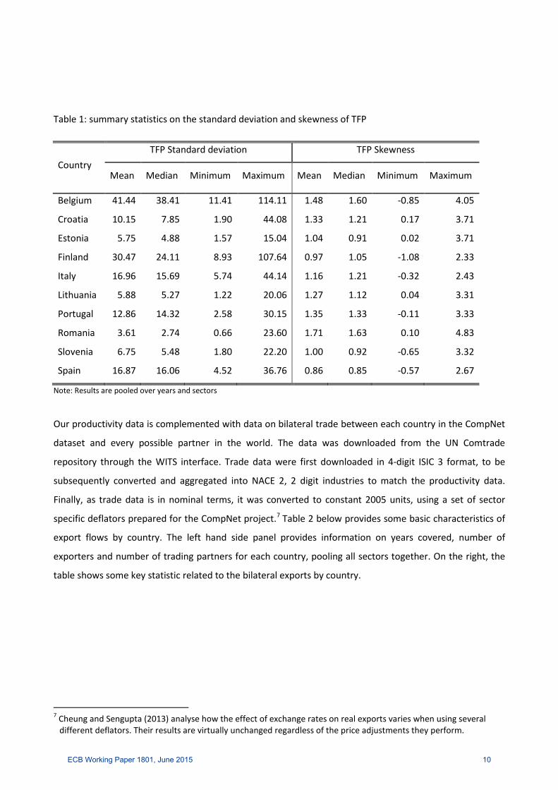
Table 1: summary statistics on the standard deviation and skewness of TFP

Country TFP Standard deviation TFP Skewness

Mean Median Minimum Maximum Mean Median Minimum Maximum

Belgium 41.44 38.41 11.41 114.11 1.48 1.60 -0.85 4.05

Croatia 10.15 7.85 1.90 44.08 1.33 1.21 0.17 3.71

Estonia 5.75 4.88 1.57 15.04 1.04 0.91 0.02 3.71

Finland 30.47 24.11 8.93 107.64 0.97 1.05 -1.08 2.33

Italy 16.96 15.69 5.74 44.14 1.16 1.21 -0.32 2.43

Lithuania 5.88 5.27 1.22 20.06 1.27 1.12 0.04 3.31

Portugal 12.86 14.32 2.58 30.15 1.35 1.33 -0.11 3.33

Romania 3.61 2.74 0.66 23.60 1.71 1.63 0.10 4.83

Slovenia 6.75 5.48 1.80 22.20 1.00 0.92 -0.65 3.32

Spain 16.87 16.06 4.52 36.76 0.86 0.85 -0.57 2.67

Note: Results are pooled over years and sectors

Our productivity data is complemented with data on bilateral trade between each country in the CompNet

dataset and every possible partner in the world. The data was downloaded from the UN Comtrade

repository through the WITS interface. Trade data were first downloaded in 4-digit ISIC 3 format, to be

subsequently converted and aggregated into NACE 2, 2 digit industries to match the productivity data.

Finally, as trade data is in nominal terms, it was converted to constant 2005 units, using a set of sector

specific deflators prepared for the CompNet project.7 Table 2 below provides some basic characteristics of

export flows by country. The left hand side panel provides information on years covered, number of

exporters and number of trading partners for each country, pooling all sectors together. On the right, the

table shows some key statistic related to the bilateral exports by country.

7 Cheung and Sengupta (2013) analyse how the effect of exchange rates on real exports varies when using several

different deflators. Their results are virtually unchanged regardless of the price adjustments they perform.


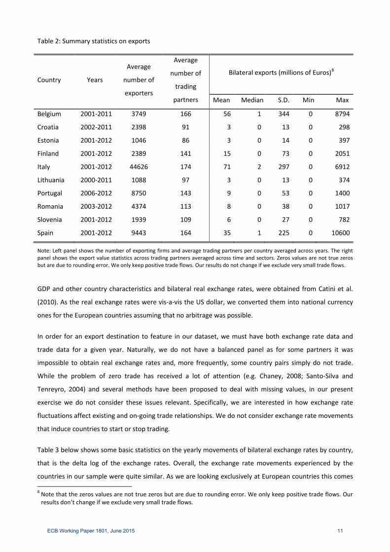
Table 2: Summary statistics on exports

Country Years

Average

number of

exporters

Average

number of

trading

partners

Bilateral exports (millions of Euros)8

Mean Median S.D. Min Max

Belgium 2001-2011 3749 166 56 1 344 0 8794

Croatia 2002-2011 2398 91 3 0 13 0 298

Estonia 2001-2012 1046 86 3 0 14 0 397

Finland 2001-2012 2389 141 15 0 73 0 2051

Italy 2001-2012 44626 174 71 2 297 0 6912

Lithuania 2000-2011 1088 97 3 0 13 0 374

Portugal 2006-2012 8750 143 9 0 53 0 1400

Romania 2003-2012 4374 113 8 0 38 0 1017

Slovenia 2001-2012 1939 109 6 0 27 0 782

Spain 2001-2012 9443 164 35 1 225 0 10600

Note: Left panel shows the number of exporting firms and average trading partners per country averaged across years. The right panel shows the export value statistics across trading partners averaged across time and sectors. Zeros values are not true zeros but are due to rounding error. We only keep positive trade flows. Our results do not change if we exclude very small trade flows.

GDP and other country characteristics and bilateral real exchange rates, were obtained from Catini et al.

(2010). As the real exchange rates were vis-a-vis the US dollar, we converted them into national currency

ones for the European countries assuming that no arbitrage was possible.

In order for an export destination to feature in our dataset, we must have both exchange rate data and

trade data for a given year. Naturally, we do not have a balanced panel as for some partners it was

impossible to obtain real exchange rates and, more frequently, some country pairs simply do not trade.

While the problem of zero trade has received a lot of attention (e.g. Chaney, 2008; Santo-Silva and

Tenreyro, 2004) and several methods have been proposed to deal with missing values, in our present

exercise we do not consider these issues relevant. Specifically, we are interested in how exchange rate

fluctuations affect existing and on-going trade relationships. We do not consider exchange rate movements

that induce countries to start or stop trading.

Table 3 below shows some basic statistics on the yearly movements of bilateral exchange rates by country,

that is the delta log of the exchange rates. Overall, the exchange rate movements experienced by the

countries in our sample were quite similar. As we are looking exclusively at European countries this comes 8 Note that the zeros values are not true zeros but are due to rounding error. We only keep positive trade flows. Our

results don’t change if we exclude very small trade flows.


as little surprise, as they are likely to be exposed to common shocks vis-a-vis third parties. What stands out

in Table 3 is the difference between old and new EU countries. While for Belgium and Finland the average

change in the exchange rate has been below 1%, for countries such as Romania, Estonia and Lithuania, it

has been over 3 %. Also of interest is that in our sample, with the exception of Portugal, all countries had a

negative average change in the exchange rate, indicating increasing in price competitiveness. For mature

EU countries, this is likely due to the initial devaluation of the Euro in the first part of the 2000s. For Central

and Eastern European (CEE) countries, it is likely due to EU accession. Mature EU countries had a roughly

equal share of appreciation and depreciation episodes while for CEE countries, only about a third of

bilateral relationships were appreciation, going as low as about 26 % in the case of Romania. Nonetheless,

for all countries the standard deviation was between 8 and 10%, indicating a rather stable exchange rate.

Table 3: Statistics on the movements of the exchange rate

Delta Exchange rate Share of

Mean Median S.D. Appreciation depreciation

Belgium -0.63% 0.01% 9.37% 50.19% 49.81%

Croatia -1.75% -1.07% 8.02% 41.97% 58.03%

Estonia -3.41% -2.82% 8.11% 27.26% 72.74%

Finland -0.35% 0.37% 9.18% 53.58% 46.42%

Italy -0.94% -0.26% 9.61% 47.16% 52.84%

Lithuania -3.60% -2.30% 8.11% 30.32% 69.68%

Portugal 2.01% 1.01% 8.10% 57.10% 42.90%

Romania -5.20% -6.14% 8.96% 26.44% 73.56%

Slovenia -2.07% -0.81% 8.69% 40.90% 59.10%

Spain -1.38% -1.04% 9.75% 40.53% 59.47%

Note: The table for each country shows the statistics on bilateral exchange rates pooled overall trade partners and years in the sample

4.2. Empirical specification

In order to estimate the elasticity of exports on the exchange rate we start from a standard gravity

equation where we have exports on the left hand side, countries’ GDPs and bilateral controls on the right

hand side, along with our variables of interest: the real exchange rate and productivity statistics terms

interacted with the exchange rate.

(1) ln�𝑋𝑛𝑛,𝑡𝑗 � =

𝛼 + 𝛽𝛽𝛽�𝑅𝑅𝑅𝑛𝑛,𝑡�+ 𝛾𝛽𝛽�𝑅𝑅𝑅𝑛𝑛,𝑡�× ln𝑃𝑃𝑃𝑃 𝐷𝑛,𝑡𝑗 + 𝜎𝛽𝛽�𝑅𝑅𝑅𝑛𝑛,𝑡� × ln𝑃𝑃𝑃𝑃 𝑆𝑛,𝑡

𝑗 +

𝜍1 ln𝑃𝑃𝑃𝑃 𝑆𝑛,𝑡𝑗 + 𝜍2 ln𝑃𝑃𝑃𝑃 𝐷𝑛,𝑡

𝑗 + 𝛿1𝐷𝑛𝑛,𝑡𝑗 + 𝛿2𝐺𝐷𝑃𝑛,𝑡 + 𝛿3𝐺𝐷𝑃𝑛,𝑡 + 𝑐𝑃𝛽𝑐𝑃𝑃𝛽𝑐𝑛𝑛

𝑗 + 𝜀𝑛𝑛,𝑡𝑗


Where n denotes the exporting country, i the importing one, j the sector and t is the year. On the left hand

side of the equation, we have the log change in bilateral exports; on the right hand side, RER denotes the

bilateral real exchange rate between the two countries, D is a pair and sector specific demand shifter,

whose construction is detailed below. Prod S and Prod D are productivity distribution higher order statistics

we will be looking at. The regression contains both importer and exporter GDP to control for the relative

size of the economies.

Since our interest also lies in the non-linear response of exports to exchange rate fluctuations, we estimate

our model in first differences. This estimation strategy is a popular approach in the literature (see Bahmani-

Oskooee and Ratha (2008) for an overview, likely due to the time-series focus that this research has

traditionally adopted. However, there are panel-setting approaches, which also run the models in first

differences, such as Cheung and Sengupta (2013).

Note that by taking the first difference of the equation above, the standard gravity controls, such as

distance or common border, drop out. The same is true for whatever sector and country fixed effects we

may also wish to include. Finally, other typical gravity controls such as population vary too little from year

to year and we do not include them9. The first difference specification we will run is equation (2), where

our variables of interest are β, 𝛾1 and 𝜎1 9F

10. Our benchmark specification is very similar to the sector level

regression in Berman et al. (2012) and to the first difference one in Cheung and Sengupta (2013).

(2) Δln�𝑋𝑛𝑛,𝑡𝑗 � = 𝛼 + 𝛽Δ𝛽𝛽�𝑅𝑅𝑅𝑛𝑛,𝑡�+ 𝛾1Δ𝛽𝛽�𝑅𝑅𝑅𝑛𝑛,𝑡� × ln𝑃𝑃𝑃𝑃 𝐷𝑛,𝑡

𝑗 + 𝛾1Δ𝛽𝛽�𝑅𝑅𝑅𝑛𝑛,𝑡� ×

ln𝑃𝑃𝑃𝑃 𝐷𝑛,𝑡𝑗 + 𝜎1Δln�𝑅𝑅𝑅𝑛𝑛,𝑡�× ln𝑃𝑃𝑃𝑃 𝑆𝑛,𝑡

𝑗 +

𝛾2𝛽𝛽�𝑅𝑅𝑅𝑛𝑛,𝑡�× Δln𝑃𝑃𝑃𝑃 𝐷𝑛,𝑡𝑗 + 𝛾3Δln�𝑅𝑅𝑅𝑛𝑛,𝑡�× Δln𝑃𝑃𝑃𝑃 𝐷𝑛,𝑡

𝑗 + 𝜎2𝛽𝛽�𝑅𝑅𝑅𝑛𝑛,𝑡�

× Δln𝑃𝑃𝑃𝑃 𝑆𝑛,𝑡𝑗 + 𝜎3Δ𝛽𝛽�𝑅𝑅𝑅𝑛𝑛,𝑡� × Δln𝑃𝑃𝑃𝑃 𝑆𝑛,𝑡

𝑗 +

𝛿1Δ𝐷𝑛𝑛,𝑡𝑗 + 𝛿2Δ𝐺𝐷𝑃𝑛,𝑡 + 𝛿3Δ𝐺𝐷𝑃𝑛,𝑡 + Δ𝜀𝑛𝑛,𝑡

𝑗

In order to control for foreign demand, we construct a trade weighted measure of foreign income similar to

the one used in the literature to construct industry specific real effective exchange rates (Goldberg, 2004).

For country pair in at time t we generate the following weights in sector j:

9 We have run versions of our equations that include exporter, importer and/or sector dummies and their interactions

as controls. Results are change little when we include country, time or sector fixed effect in the regression, bar for a slightly higher R2 statistic.

10 We freely admit that the specification appears to be cumbersome but the first difference specification must take into account changes in all pairs of interacted variables. We tried running a simpler version of equation (2), without the cross-product terms and the results don’t change in any meaningful way. However, as the estimates are numerically different we decided to keep the full specification.


(3) jtn

jtn

jtni

jtnit

ij

tni XXXX

GDPD1,,

1,,,

−

−

++

=

Where jtniX , are bilateral exports at time t and j

tnX , are total exports at time t. We average over two

consecutive years in order to smooth out any transitory shocks.

Ideally, we would like to control for both dispersion and skewness but it is instructive to see how the

results change when one or both statistics are not included. Therefore, we have four specifications: a basic

one where we don't control for any sectorial characteristics (that is, the γ and σ terms are absent), one

which controls for the skewness of TFP, one which controls for the dispersion of TFP and one which

controls for both these effects. Our preferred specification is the latter as it controls for both higher order

characteristics of the productivity distribution.

In terms of data clean up, we remove observations pairs, when the exchange rate moves by more than 50%

in one direction or another in a given year. This has a minimal effect since it causes the drop of only around

2000 observations. We further drop from the analysis sectors with fewer than 20 firms, as these sectors are

unlikely to have robust skewness and dispersion statistics. Also, in order to have results comparable across

specifications, we drop observations than have all variables present, regardless if the variables are required

in that particular specification.

Results

5.1 Benchmark results

In this section, we present the results of our specifications without taking into account any of the non-

linear effects discussed in the introduction. The main variables of interest are presented in the first three

rows of Table 4. Column (1) shows the results without taking into account any of the higher moment of the

productivity distribution. The results indicate that a 10% depreciation of the exchange rate would boost

exports by about 3%. Column (2) shows the results, when taking into account the dispersion of

productivity. Two aspects stand out: the coefficient of the interaction term is positive and statistically

significant, indicating lower elasticity in sectors where firms are most productive. Second, when including

sector specific productivity dispersion statistics, the baseline elasticity changes, more than doubling. We

also find there is substantial variation in the response of sectors depending on their productivity

distribution: standard deviation of TFP significantly associated with lower exchange rate elasticity. In the

context of our data, a higher TFP standard deviation implies a fatter right tail for the productivity

distribution and a distribution shifted more to the right, i.e. a more performing sector. Table 5 presents the

country and sector specific exchange rate elasticity estimates, showing substantial variation both within


and across countries. The distribution across countries is highly reminiscent of the one in Table 3 in that

elasticities tend to be higher in Southern and Eastern European countries. This is expected, though, as the

estimated elasticities are a log-linear function of productivity dispersion.

Table 4: Regression of delta log exchange rates on exchange rates without taking into account non-linear characteristics

(1) (2) (3) (4)

Δln(XR) -0.356*** -0.774*** -0.355*** -0.773***

(0.0355) (0.129) (0.0357) (0.129)

Δln(XR) × ln(TFP) dispersion 0.157*** 0.157***

(0.0434) (0.0435)

Δln(XR) × ln(TFP) skewness -0.0121 -0.0173

(0.0456) (0.0461)

Δln(TFP) dispersion × Δln(XR) -0.528 -0.548

(0.292) (0.315)

Δln(TFP) dispersion × ln(XR) 0.0227*** 0.0323***

(0.00700) (0.00749)

Δln(TFP) skewness × Δln(XR) -0.0180 0.0327

(0.0921) (0.0985)

Δln(TFP) skewness × ln(XR) -0.00410** -0.00815***

(0.00208) (0.00223)

ΔForeign Demand 0.00258*** 0.00257*** 0.00258*** 0.00257***

(0.000179) (0.000179) (0.000179) (0.000178)

Δln(GDPn) 1.404*** 1.379*** 1.402*** 1.371***

(0.0860) (0.0863) (0.0860) (0.0863)

Δln(GDPi) 1.444*** 1.423*** 1.444*** 1.413***

(0.109) (0.110) (0.109) (0.110)

Observations 172,501 172,501 172,501 172,501

R-squared 0.008 0.008 0.008 0.008

*** p<0.01, ** p<0.05

Robust standard errors in parentheses. Allowing for various patterns of error clustering (by exporter/importer/sector or

various combinations) does not affect the significance of results in any meaningful way, albeit for higher p-values.

Column (3) shows the results controlling for TFP skewness. The estimated exchange rate elasticity is not

very different from the one in column (1) and the coefficient on skewness interaction is not significant.

Finally, column (4) which is our preferred specification controls for both skewness and dispersion. These

results are almost identical to those of column (2).


One puzzling result of our estimation is that skewness (line 3 in the table) has virtually zero impact on

export elasticity. This result consistently appears in all our specifications. In appendix I, we discuss why the

skewness may not be a good indicator of export performance and provide several stylized examples in this

regard. From a more technical point of view, since the shape of the distributions is similar across sectors

and countries, we may simply do not observe enough variation in order to identify the coefficient.

Nonetheless, we choose to retain skewness in the list of covariates as its inclusion adds extra information,

albeit in a non-straightforward fashion, on the sectors’ underlying productivity distributions and its

inclusion affects the magnitude of the other variables, alleviating potential bias. The variables in the middle

of Table 3 are only included because they result from the mathematical derivation of the first difference. As

mentioned previously, including or excluding them has a negligible effect on the sign and magnitude of the

other covariates. They are, however, difficult to interpret and will not be commented upon.

The last three variables in Table 4 measure changes in foreign and domestic demand and have the

expected signs. The coefficients related to GDP are significant and equal to about 1.4 across the various

specifications, a value, which is in line with previous estimations of gravity models11.

11 See Anderson and van Wincoop (2004) for a thorough survey of the gravity literature.


Table 5: country and sector specific elasticity estimates

Sector BE EE ES FI FR HR IT LT PT RO SI

Manufacture of food products -63.5% -34.1% -24.2% -38.3% -44.4% -41.5% -49.4% -41.4% -71.7% -52.0% -63.5%

Manufacture of beverages -42.3% -42.8% -46.7% -37.9% -48.0% -37.6% -64.8%

Manufacture of textiles -51.7% -30.9% -16.9% -18.8% -41.1% -30.2% -42.4% -50.2% -59.2% -42.7% -51.7%

Manufacture of wearing apparel -57.5% -31.7% -16.6% -17.4% -47.1% -29.8% -59.6% -57.1% -59.6% -53.8% -57.5%

Manufacture of leather and related products -53.1% -31.5% -28.6% -27.5% -41.1% -29.7% -51.4% -59.3% -50.6% -53.1%

Manufacture of wood and of products of wood and cork, except furniture -56.0% -51.2% -31.1% -50.4% -48.5% -39.9% -51.6% -53.1% -65.9% -57.8% -56.0%

Manufacture of paper and paper products -22.6% -18.4% -33.1% -39.8% -19.2% -36.2% -33.5% -62.6% -38.7%

Printing and reproduction of recorded media -39.2% -31.3% -33.8% -24.5% -38.9% -25.2% -48.9% -39.6% -51.5% -43.7% -39.2%

Manufacture of chemicals and chemical products -42.9% -41.9% -28.3% -26.4% -47.9% -33.4% -47.4% -32.2% -60.5% -52.3% -42.9%

Manufacture of basic pharmaceutical products and pharmaceutical preparations -29.4% -12.3% -24.3% -25.3% -46.3%

Manufacture of rubber and plastic products -60.6% -41.7% -27.8% -53.2% -54.6% -48.9% -63.9% -62.1% -79.8% -61.4% -60.6%

Manufacture of other non-metallic mineral products -63.8% -42.2% -28.7% -35.9% -61.9% -44.8% -67.2% -55.4% -77.3% -63.7% -63.8%

Manufacture of basic metals -32.1% -27.6% -30.0% -53.5% -37.7% -40.3% -60.1% -45.3%

Manufacture of fabricated metal products, except machinery and equipment -62.7% -36.3% -28.6% -34.2% -56.4% -45.1% -57.1% -56.5% -68.2% -63.2% -62.7%

Manufacture of computer, electronic and optical products -41.7% -33.8% -13.0% -21.4% -31.9% -31.7% -40.7% -26.8% -50.1% -36.3% -41.7%

Manufacture of electrical equipment -42.9% -27.7% -15.8% -25.3% -29.2% -28.9% -49.1% -29.2% -47.6% -34.8% -42.9%

Manufacture of machinery and equipment -43.9% -26.3% -23.6% -27.3% -37.2% -32.0% -48.7% -33.3% -59.9% -45.3% -43.9%

Manufacture of motor vehicles, trailers and semitrailers -25.1% -30.9% -39.3% -38.5% -32.2% -31.0% -60.4% -48.2%

Manufacture of other transport equipment -28.3% -12.8% -16.6% -25.8% -39.8% -35.8% -35.3%

Manufacture of furniture -60.2% -40.4% -39.6% -26.9% -54.1% -36.2% -62.3% -33.4% -71.0% -62.9% -60.2%

Other manufacturing -45.3% -37.0% -40.4% -26.2% -48.8% -34.2% -57.9% -31.7% -69.4% -54.3% -45.3%

Repair and installation of machinery and equipment -49.9% -38.3% -32.6% -21.8% -44.9% -37.1% -59.5% -31.8% -62.7% -51.6% -49.9%

Note: Estimates are obtained by adding the base elasticity and multiplying the log of each sector’s TFP standard deviation by the interaction coefficient obtained in Table 4. The results are averaged over time. This does not mean, though, that the elasticities are constant over time. Splitting the sample in two, we find substantially higher elasticities in the first half of the 2000 than afterwards, an effect already documented in Di Mauro et al (2008). We do not pursue this further in the paper.


Our baseline elasticity of exports increases to 77%, a figure in line with the broad literature (see Table 6 for

some comparable estimates). Our results also confirm the findings in Dekle et al. (2009), in that accounting

for productivity statistics alleviates the bias towards zero in macroeconomic regressions and our results are

numerically close to theirs and to those in Berthou (2008). Our results are qualitatively similar to Berman et

al. (2012), who run a similar regression, albeit in levels, interacting real exchange rate movements with

sector level productivity dispersion. They find an elasticity of almost 90% and that more heterogeneous

sectors are less sensitive to exchange rate movements. The heterogeneity estimates have the same sign,

but they cannot be directly compared as they proxy productivity dispersion by a Herfindahl index of

concentration and an estimated Pareto parameter fitted to the underlying sector distribution. This

difference in approaches could possibly explain their higher elasticity parameters as the fatter tails of the

Pareto distribution may bias the results upwards.

Table 6: Sample of exchange rate elasticity estimates in the literature

Source Bilateral elasticity estimate

Berthou (2008)

Berman et al. (2013)

Bun and Klassen (2014)

Dekle et al. (2009)

68%

40-91%

56%

41-71%

Note: The table includes only the estimates that were derived in a manner comparable to the one in this paper.

A key result is how much the elasticity estimates change when properly accounting for heterogeneity.

However, not controlling in any way for variations across countries and sectors is not a fair benchmark.

Assuming no other information is available besides trade and exchange rate data, the easiest way to

account for variability is to include sector and country dummies and let them interact with the exchange

rate elasticity estimates. This approach has two drawbacks, though. First, sectors and countries vary by

more than just productivity and the dummies capture all these distinct characteristics, obfuscating the

effect of productivity variation. Second, by including dummies, we restrict the observed variability we

observe, forcing us to rely more on the time dimension for identification, which in our case involves a

rather short panel. We run nevertheless several versions of these dummy augmented regressions and

summarize them in Table 7. The last column shows our preferred estimates for comparison.

Several results emerge. First, the R2 does not change between models. Second, while including dummies

has the advantage of producing sector and country specific estimates, these estimates lack reliability: for

most counties the sector/country specific estimates are statistically indistinguishable from the average


effect12. Third, and somewhat surprising, while including sectors dummies reduces the zero bias in the

elasticity estimates, including exporter dummies actually brings the coefficient closer to zero and including

both effects has no effect on the baseline elasticity estimates.

Table 7: Exchange rate base estimates under various controls

VARIABLES (1) (2) (3) (4) (5)

Δln(XR) -0.356*** -0.463*** -0.208*** -0.357** -0.773***

(0.0338) (0.143) (0.0730) (0.154) (0.129)

Δln(XR)

interacted with

No

controls

sector

dummies

exporter

dummies

sector and exporter

dummies

Productivity

moments

Observations 172,501 172,501 172,501 172,501 172,501

R-squared 0.008 0.008 0.008 0.009 0.008

Note: All other covariates are included in the estimation. Robust standard errors in parentheses; *** p<0.01, ** p<0.05

4.3. Asymmetry

While we expect a depreciation to boost exports and an appreciation to inhibit them, the two effects need

not be the mirror image of each other. In order to more easily compare our results between the two cases,

we specify our regression such that the elasticity coefficients associated with depreciations to have the

same sign as the one associated to appreciation. However, as mentioned in section 2, we expect them to

have different magnitudes. In order to test this hypothesis, we let the interact the RER coefficients in

equation (2), β, 𝛾1 and 𝜎1, with dummies indicating the sign of the exchange rate movement.

As in the benchmark, we run four specifications, in turn including TFP dispersion and skewness as

asymmetry measures. Our preferred specification is the one including both of them. The results are

summarized in Table 8 where the first three rows show the estimates for the variables of interest during

appreciation episodes and the next three rows show them during depreciation episodes. We will only focus

on columns (1) and (4) as including skewness by itself has no impact on the estimates and column (4) is

virtually identical to column (2). Column (1) shows the results without taking into account any productivity

distribution statistics. In the case of appreciation the coefficient is significant and with the right sign.

For depreciations instead, as in Dekle et al. (2009) the baseline elasticity estimate has the wrong sign and is

highly significant. Our result further stresses the need to include productivity statistics in order to obtain

accurate estimates. Including dispersion statistics helps the elasticity identification. For appreciations, the

elasticity tends to be higher than zero. For depreciations, the estimates tend to be close to zero and with

12 These full list of estimates are not shown here but are available on request.


the correct sign. In our preferred specification, column (4) which includes both productivity distribution

statistics, we find that the impact in the case of appreciation is both statistically significant and substantially

meaningful. That is, a 10% RER increase will decrease the value of exports by 10%. Meanwhile, currency

depreciation will not have a noticeable effect on exports. We also find that in countries and sectors with

higher TFP dispersion the RER fluctuations are less pronounced. These results are in line with our

expectation and the theoretical motives described in the introduction.


Table 8: Regression of delta exports on exchange rates taking into account the sign of the shock

(1) (2) (3) (4)

Appreciation

Δln(XR) -0.761*** -1.011*** -0.759*** -1.006***

(0.0515) (0.150) (0.0519) (0.150)

Δln(XR) × ln(TFP) dispersion 0.0995** 0.0995**

(0.0503) (0.0504)


(0.0559) (0.0563)

Depreciation

Δln(XR) 0.217*** -0.208 0.215*** -0.212

(0.0746) (0.261) (0.0747) (0.263)

Δln(XR) × ln(TFP) dispersion 0.148 0.148

(0.0840) (0.0851)

Δln(XR) × ln(TFP) skewness 0.0190 0.0244

(0.0790) (0.0806)


(0.292) (0.315)


(0.00702) (0.00753)


(0.0921) (0.0985)

Δln(TFP) skewness × ln(XR) -0.00388 -0.00789***

(0.00208) (0.00223)

ΔForeign Demand 0.00258*** 0.00258*** 0.00258*** 0.00257***

(0.000179) (0.000179) (0.000179) (0.000179)

Δln(GDPn) 1.426*** 1.407*** 1.425*** 1.399***

(0.0858) (0.0864) (0.0858) (0.0865)

Δln(GDPi) 1.278*** 1.257*** 1.280*** 1.251***

(0.112) (0.113) (0.112) (0.113)

Observations 172,501 172,501 172,501 172,501

R-squared 0.008 0.008 0.008 0.009

*** p<0.01, ** p<0.05

Robust standard errors in parentheses. Allowing for various patterns of error clustering (by exporter/importer/sector or various

combinations) does not affect the significance of results in any meaningful way, albeit for higher p-values. In some combinations

the interaction term between dispersion and appreciation becomes insignificant.


Note: In line with the literature, we expect depreciation to boost exports and appreciation to inhibit them. Despite these opposite

effects, in our specification, the elasticity coefficients in the two cases should have the same sign if we are to believe this

hypothesis. In other words, for appreciation, we look at the difference in effect between a 2% and 3% appreciation and for

depreciation we look at the difference in effect between a -3% and -2% depreciation.

4.4. Large changes

In this section, we investigate the hypothesis that exporters are more likely to react to large changes in the

exchange rate than to small ones. As we are looking at the effects of exchange rate over the relatively short

run, we expect there to be differences in the response of firms depending on the size of the shock due to

adjustment rigidities. As contracts are negotiated in advance and setting a distribution network is costly,

prices and quantities are sticky in the short term and a firm may choose not to optimally adjust

immediately following an exchange rate fluctuation and may allow its mark-up to absorb some of the

losses. However, a large change in exchange rate may make it much too unprofitable to stick to this course

of action and may induce the firm to change its prices or quantities.

We define as small shocks those lying between the 10th and 90th percentile of changes in the exchange rate.

This way, half of the exchange rate movements in our sample will be considered large and half of them will

be considered small. Numerically, this classifies movements between 9% depreciation and 12%

appreciation as small. This is much larger than what is considered in the exchange rate pass through

literature: for instance, Bussiere (2006) considers small movements being +/- 3%.

Table 9 shows the estimated elasticities allowing them to differ depending on the classification of the

shock. The first block of estimates, under the header “Small” indicate the elasticities in the case of central

80% movements in the exchange rate while those under the header “Large shocks” indicate the estimates

in the outer 20% of movements. As usual, the first column shows the estimates without taking into account

any productivity characteristics. The elasticities for both small and large shocks are statistically significant,

and for small shocks, the elasticity estimate is smaller, as expected. Taking into account the standard

deviation of TFP, the results change drastically. The elasticity estimates for both small and large shocks

increases, but more for the large ones. In the case of large exchange rate movements, we also observe that

the more dispersed sectors have a lower elasticity of exports. Including the productivity skewness has a

minimal impact on the estimated coefficients. We tried different thresholds for the definition of large

shocks and the more extreme the events the larger the elasticity estimates we obtained. This makes sense

as we are now able to capture adjustments on the extensive not just the intensive side: larger shocks will

not only generate stronger responses but also will cause marginal firms to adjust their exports, amplifying

the observed elasticity (remember we only observe trade variables at the sector level).


Table 9: Regression of delta log exchange rates on exchange rates taking into account the size of the shock

(1) (2) (3) (4)

Small shocks

Δln(XR) -0.294*** -0.512** -0.289*** -0.511**

(0.0697) (0.234) (0.0705) (0.234)

Δln(XR) × ln(TFP) dispersion 0.0831 0.0843

(0.0794) (0.0797)


(0.0949) (0.0953)

Large shock

Δln(XR) -0.375*** -0.866*** -0.374*** -0.865***

(0.0407) (0.152) (0.0409) (0.152)

Δln(XR) × ln(TFP) dispersion 0.183*** 0.183***

(0.0511) (0.0513)


(0.0524) (0.0530)


(0.293) (0.316)


(0.00700) (0.00749)


(0.0923) (0.0988)

Δln(TFP) skewness × ln(XR) -0.00408 -0.00813***

(0.00208) (0.00223)

ΔForeign Demand 0.00258*** 0.00258*** 0.00258*** 0.00257***

(0.000179) (0.000179) (0.000179) (0.000179)

Δln(GDPn) 1.404*** 1.381*** 1.402*** 1.372***

(0.0860) (0.0863) (0.0860) (0.0864)

Δln(GDPi) 1.443*** 1.418*** 1.444*** 1.409***

(0.109) (0.110) (0.109) (0.110)

Observations 172,501 172,501 172,501 172,501

R-squared 0.008 0.008 0.008 0.008

*** p<0.01, ** p<0.05

Robust standard errors in parentheses. Allowing for various patterns of error clustering (by exporter/importer/sector or various

combinations) does not affect the significance of results in any meaningful way, albeit for higher p-values. In some combinations

the elasticity for small changes becomes insignificant.


5. Conclusions

This paper provides new empirical estimates of the elasticity of exports to the exchange rate. The value

added of the paper is the use of a novel database of sector productivity for a set of EU countries, derived

from firm level information. The main result is that when the underlying firm productivity distribution is

taken into consideration the elasticity estimates double in value. In addition, the more heterogeneous is

the sector - i.e. the higher is the concentration of highly productive firms - the lower is the sensitivity of

exports to exchange rates movements. Finally, reactions to exchange rate movements are not symmetric,

since what appears to matter are only appreciations – as opposed to depreciations –, as well as relatively

large – rather than small – exchange rate swings.


Appendix

Appendix I – The link between dispersion and skewness

This section provides some numerical examples to help understand the interplay between dispersion and

skewness of a right-tailed distribution, such as in the case of productivity. Let us assume two countries of

10000 firms each and all firm are exporters. For the sake of simplicity, let us assume productivity is binary:

firms can be either low productivity or high productivity. Without loss of generality, low productive firms

have productivity equal to one and high productive firms have productivity equal to 50. In country A, out of

the 10000 firms, 2000 are high productivity and 8000 are low productivity while in country B only 10 firms

are high productivity. Economically speaking, we expect the impact of exchange rate fluctuations in country

A to be much less pronounced, as there are more productive firms than in country B. However, the

statistics of the two distributions are radically different. Economy A has a standard deviation of 19.6 and a

skewness of 1.5 whereas country B has a standard deviation of 1.6 and a skewness of 30.1. It is clear that,

at least in our example, a higher standard deviation implies a larger concentration of productive firms,

while a higher skewness implies exactly the opposite.

Figure A1: Evolution of higher order statistics in a binary productivity setting

Finally, let us consider two popular distributions in the theoretical firm level literature, the Pareto and the

lognormal distribution. Both distributions have two parameters, a location and a shape parameter, and

increasing either of them makes the sector more competitive: increasing the location moves the whole

distribution more to the right while increasing the shape parameter has a stronger impact on the right tail.

0 1000 2000 3000 4000 50000

5

10

15

20

25

Number of productive firms

Sta

ndar

d D

evia

tion

0 1000 2000 3000 4000 50000

10

20

30

40

50

60

70

80

90

100


Ske

wne

ss

0 1000 2000 3000 4000 50000

5

10

15

20

25

30

35

40

45

50


Inte

rqua

rtile

rang

e

Binary productivity


Figure A2 plots the evolution of productivity standard deviation and skewness for a sector with 10000 firms

randomly drawn from a Pareto distribution. In Panel 1, we increase the scale parameter from zero to four,

whereas in panel B we increase the shape parameter from zero to two. In both cases, we keep the other

parameter constant.

Figure A2: Simulation of Pareto distributions under various scale and shape parameters.

In Figure A3, we plot the standard deviation and skewness for the lognormal distribution resulting from

simulations allowing the underlying distribution’s two parameters to vary. Again, an increase in either

parameter of the distribution would make the economy more export prone. The standard deviation

increases with an increases in an exponential fashion in both parameters but the skewness increases only

when the scale parameter increase.

Figure A3: Simulation of Lognormal distributions under various scale and location parameters.


Appendix II – Robustness check

In order to check the sensitivity of our results to our choice of productivity proxy, we repeat our previous

exercises using an alternative productivity measure: apparent labour productivity, defined as real value

added per employee. The data is also collected as part of the CompNet dataset defined in real Euros,

adjusted for value added PPPs. The same outlier and data clean up treatment as for TFP, detailed in section

3, is applied to labour productivity. Table A1 summarizes the key statistics for the standard deviation and

skewness of labour productivity for the countries covered in this paper. The country profiles are similar as

in the case of TFP. As labour productivity is directly derived from balance sheet information, it is less likely

to be affected by the implicit and explicit assumptions of the TFP estimation procedure. It is likely, though,

to be somewhat correlated, or more correlated than TFP, with other characteristics that affect exports.

Table A1: statistics on dispersion and skewness of labour productivity

Country Standard deviation Skewness

Mean Median Minimum Maximum Mean Median Minimum Maximum

Belgium 30.79 32.24 5.36 54.02 1.81 1.82 -0.28 5.92

Croatia 11.25 10.49 2.85 22.47 1.79 1.59 0.03 4.99

Estonia 6.65 6.27 2.10 13.85 1.29 1.21 -0.51 3.44

Finland 30.78 27.72 5.81 72.45 2.15 2.09 -0.31 5.78

Italy 16.24 16.69 5.07 26.51 1.17 1.20 -0.09 2.55

Lithuania 5.60 5.62 1.15 10.12 1.32 1.26 0.10 4.26

Portugal 9.57 11.13 1.66 15.35 0.84 0.86 -0.80 2.29

Romania 4.61 4.34 1.60 8.97 1.71 1.59 -0.63 4.40

Slovenia 6.25 5.67 1.66 13.82 1.39 1.39 -0.15 2.92

Spain 16.76 17.59 4.99 25.22 1.09 1.08 0.22 2.13

Note: Results are pooled over years and sectors

Estimation

We repeat all the exercises in section 4 without changing anything but the productivity measure. This

approach is likely to produce biased results as export sales are part of the construction of the value added

variable. Moreover, value added, as it is an accounting concept, is more likely that TFP to be influenced by

other unobserved factors.

The estimates in column (1) of Table A2 are identical to the ones in Tables 7, as they are the simplest form

of regression without including any of our productivity statistics. The following two columns include, in


turn, productivity dispersion and skewness statistics and column (4) includes both measures. When taking

into account these additional covariates, the elasticity estimates change drastically, and the heterogeneous

effect due to dispersion across sectors is about as pronounced as in the case of TFP regression. Puzzlingly,

the skewness results are negative and statistically significant, indicating the sectors with a long productivity

right tail are more sensitive to exchange rate movements.

In the case of asymmetric shocks, Table A3, our labour productivity results are again similar to the TFP

ones: including sector characteristics drastically changes the estimated elasticity, although the estimated

elasticities are lower than for TFP. Interestingly, for depreciation, an increase in productivity dispersion

lowers the elasticity by 20% although the baseline elasticity estimate is not statistically significant. We

suspect that the elasticity point estimate is different from zero but we do not have enough variation in our

sample to pinpoint the exact value. What is more puzzling is that the skewness coefficients is significant in

the case of appreciation but again has the opposite signs than expected.

Finally, in Table A4 we once again split the sample into large and small shocks, using the same rules as in

the TFP section. For small shocks, neither the baseline elasticity nor the productivity interactions are

significant.


Table A2: Regression of delta log exchange rates on exchange rates without taking into account any non-linear response of exchange rates

(1) (2) (3) (4)

Δln(XR) -0.331*** -0.821*** -0.286*** -0.765***

(0.0340) (0.144) (0.0409) (0.146)

Δln(XR) × ln(lprod SD) 0.181*** 0.177***

(0.0485) (0.0484)

Δln(XR) × ln(lprod skewness) -0.154** -0.146**

(0.0713) (0.0713)

Δln(lprod SD) × Δln(XR) -0.509** -0.534

(0.251) (0.279)

Δln(lprod SD) × ln(XR) 0.0301*** 0.0411***

(0.00585) (0.00653)

Δln(lprod skewness) × Δln(XR) 0.0540 0.110

(0.123) (0.135)

Δln(lprod skewness) × ln(XR) -0.00354 -0.0110***

(0.00240) (0.00269)

ΔForeign Demand 0.00209*** 0.00208*** 0.00209*** 0.00208***

(0.000249) (0.000248) (0.000249) (0.000248)

Δln(GDPn) 1.427*** 1.397*** 1.422*** 1.381***

(0.0821) (0.0823) (0.0821) (0.0825)

Δln(GDPi) 1.515*** 1.476*** 1.517*** 1.472***

(0.105) (0.105) (0.105) (0.105)

Observations 187,225 187,225 187,225 187,225

R-squared 0.008 0.008 0.008 0.008

*** p<0.01, ** p<0.05

Robust standard errors in parentheses. Allowing for various patterns of error clustering (by

exporter/importer/sector or various combinations) does not affect the significance of results in any meaningful

way, albeit for higher p-values.


Table A3: Regression of delta log exchange rates on exchange rates taking into account asymmetric effects

(1) (2) (3) (4) Appreciation

Δln(XR) -0.749*** -0.986*** -0.668*** -0.890***

(0.0489) (0.165) (0.0566) (0.167)

Δln(XR) × ln(lprod SD)

0.0933* 0.0883

(0.0557) (0.0556)

Δln(XR) × ln(lprod skewness)

-0.242*** -0.242***

(0.0849) (0.0849)

Depreciation

Δln(XR) 0.267*** -0.300 0.241*** -0.343

(0.0721) (0.299) (0.0806) (0.301)

Δln(XR) × ln(lprod SD) 0.195** 0.201**

(0.0961) (0.0961)

Δln(XR) × ln(lprod skewness) 0.101 0.105

(0.120) (0.120)

Δln(lprod SD) × Δln(XR) -0.417 -0.455

(0.251) (0.279) Δln(lprod SD) × ln(XR) 0.0300*** 0.0410***

(0.00587) (0.00655) Δln(lprod skewness) × Δln(XR) 0.0495 0.104

(0.123) (0.135) Δln(lprod skewness) × ln(XR) -0.00278 -0.0102***

(0.00243) (0.00272) ΔForeign Demand 0.00209*** 0.00208*** 0.00209*** 0.00208***

(0.000248) (0.000248) (0.000248) (0.000248) Δln(GDPn) 1.448*** 1.426*** 1.444*** 1.411***

(0.0818) (0.0824) (0.0818) (0.0825) Δln(GDPi) 1.340*** 1.298*** 1.369*** 1.319***

(0.107) (0.108) (0.108) (0.109) Observations 187,225 187,225 187,225 187,225 R-squared 0.009 0.009 0.009 0.009 *** p<0.01, ** p<0.05


exporter/importer/sector or various combinations) does not affect the significance of results in any

meaningful way, albeit for higher p-values.


Table A4: Regression of delta log exchange rates on exchange rates taking into the size of the shock

(1) (2) (3) (4)

Small shocks

Δln(XR) -0.306*** -0.597** -0.246*** -0.512

(0.0676) (0.259) (0.0765) (0.263)

Δln(XR) × ln(lprod SD) -0.215 -0.212

(0.127) (0.127)

Δln(XR) × ln(lprod skewness) 0.109 0.101

(0.0884) (0.0884)

Large shock

Δln(XR) -0.339*** -0.900*** -0.299*** -0.854***

(0.0388) (0.170) (0.0473) (0.172)

Δln(XR) × ln(lprod SD) 0.206*** 0.203***

(0.0572) (0.0571)

Δln(XR) × ln(lprod skewness) -0.133 -0.123

(0.0835) (0.0835)

Δln(lprod SD) × Δln(XR) -0.516** -0.544

(0.252) (0.281)

Δln(lprod SD) × ln(XR) 0.0301*** 0.0412***

(0.00585) (0.00653)

Δln(lprod skewness) × Δln(XR) 0.0557 0.113

(0.123) (0.136)

Δln(lprod skewness) × ln(XR) -0.00353 -0.0110***

(0.00240) (0.00269)

Demand 0.00209*** 0.00209***

0.00209***

0.00208***

(0.000249) (0.000248) (0.000249) (0.000249)

Δln(GDPn) 1.427*** 1.399*** 1.422*** 1.383***

(0.0821) (0.0823) (0.0821) (0.0825)

Δln(GDPi) 1.514*** 1.471*** 1.518*** 1.468***

(0.105) (0.105) (0.105) (0.105)

Observations 187,225 187,225 187,225 187,225

R-squared 0.008 0.008 0.008 0.008

*** p<0.01, ** p<0.05


exporter/importer/sector or various combinations) does not affect the significance of results in any meaningful way,

albeit for higher p-values.


References

1. Anderson, James E., and Eric Van Wincoop. Trade costs. No. 10480. National Bureau of Economic Research, 2004. 2. Atkeson, Andrew, and Ariel Burstein. "Pricing-to-Market in a Ricardian Model of International Trade." American Economic

Review 97.2 (2007): 362-367. 3. Auer, Raphael A., and Raphael S. Schoenle. Market structure and exchange rate pass-through. No. 2012-14. Swiss

National Bank, 2012. 4. Auer, Raphael A., and Raphael Schoenle. "The Mode of Competition between Foreign and Domestic Goods, Pass-

Through, and External Adjustment." (2013). 5. Bahmani-Oskooee, Mohsen, and Scott W. Hegerty. "Exchange rate volatility and trade flows: a review article." Journal of

Economic Studies 34.3 (2007): 211-255. 6. Bahmani-Oskooee, Mohsen, and Artatrana Ratha. "Exchange rate sensitivity of US bilateral trade flows." Economic

Systems 32.2 (2008): 129-141. 7. Bahmani-Oskooee, Mohsen, and Ilir Miteza. "Do nominal devaluations lead to real devaluations in LDCs?." Economics

Letters 74.3 (2002): 385-391. 8. Baldwin, Richard, and Paul Krugman. "Persistent Trade Effects of Large Exchange Rate Shocks." The Quarterly Journal of

Economics 104.4 (1989): 635-654. 9. Baxter, Marianne, and Alan C. Stockman. "Business cycles and the exchange-rate regime: some international

evidence." Journal of monetary Economics 23.3 (1989): 377-400. 10. Bee, Marco, and Stefano Schiavo. "Powerless: gains from trade when firm productivity is not Pareto distributed." (2014). 11. Bernard, Andrew B., and J. Bradford Jensen. "Why some firms export." Review of Economics and Statistics 86.2 (2004):

561-569. 12. Bernard, Andrew B., and J. Bradford Jensen. "Entry, expansion, and intensity in the US export boom, 1987–1992." Review

of International Economics 12.4 (2004): 662-675. 13. Berthou, Antoine. "An investigation on the effect of real exchange rate movements on OECD bilateral exports." (2008). 14. Antoine Berthou, Emmanuel Dhyne, Ana-Maria Cazacu and Bogdan Chiriacescu, Jaanika Merikyll, Vlad Demian, Peter 15. Harasztosi, Luca-David Opromolla, Tibor Lalinsky, Patry Tello, Matteo Bugamelli, Filippo Oropallo. “New evidence on

European exporters”, forthcoming 16. Berman, Nicolas, Philippe Martin, and Thierry Mayer. "How do different exporters react to exchange rate changes?." The

Quarterly Journal of Economics 127.1 (2012): 437-492. 17. Bugamelli, Matteo, and Luigi Infante. Sunk costs of exports. Vol. 469. Banca d'Italia, 2003. 18. Bun, Maurice JG, and Franc JGM Klaassen. "Has the Euro increased Trade?."Econometrica 82.2 (2014): 705-30. 19. Bussière, Matthieu. "Exchange rate pass-through to trade prices: the role of non-linearities and asymmetries." (2007). 20. Catini, Giulia, Ugo Panizza and Carol Saade (2010), “Macro Data 4 Stata” , http://graduateinstitute.ch/md4stata 21. Chaney, Thomas. "Distorted gravity: the intensive and extensive margins of international trade." The American Economic

Review 98.4 (2008): 1707-1721. 22. Cheung, Yin-Wong, and Rajeswari Sengupta. "Impact of exchange rate movements on exports: an analysis of Indian non-

financial sector firms." Journal of International Money and Finance 39 (2013): 231-245. 23. CompNet, E. C. B. Micro based evidence of EU competitiveness: The CompNet database. Working Paper Series 1634,

European Central Bank, 2014. 24. Connolly, Michael, and Dean Taylor. "Adjustment to devaluation with money and nontraded goods." Journal of

International Economics 6.3 (1976): 289-298. 25. Corsetti, Giancarlo, and Luca Dedola. "A macroeconomic model of international price discrimination." Journal of

International Economics 67.1 (2005): 129-155. 26. Dekle, Robert, and Kyoji Fukao. The Japan-US Exchange Rate, Productivity, and the Competitiveness of Japanese

Industries. No. 2008-25. Center for Economic Institutions, Institute of Economic Research, Hitotsubashi University, 2009. 27. Dekle, Robert, and Heajin H. Ryoo. "Exchange rate fluctuations, financing constraints, hedging, and exports: Evidence

from firm level data." Journal of International Financial Markets, Institutions and Money 17.5 (2007): 437-451. 28. Dekle, Robert, H Jeong, and Nobuhiro Kiyotaki. "Dynamics of Firms and Trade in General Equilibrium." KDI School of Pub

Policy & Management Paper 13-06 (2013). 29. Dekle, Robert, H. Jeong, and Heajin Ryoo. "A Microeconomic Analysis of the Aggregate Disconnect between Exchange

Rates and Exports." University of Southern California, mimeo (2007). 30. Delatte, Anne-Laure, and Antonia López-Villavicencio. "Asymmetric exchange rate pass-through: Evidence from major

countries." Journal of Macroeconomics 34.3 (2012): 833-844. 31. Di Mauro, Filippo, Rasmus Rüffer, and Irina Bunda. "The changing role of the exchange rate in a globalised economy." ECB

Occasional Paper 94 (2008). 32. Edwards, Sebastian. "Exchange rate misalignment in developing countries. "The World Bank Research Observer 4.1

(1989): 3-21. 33. Edwards, Sebastian, and Eduardo Levy Yeyati. "Flexible exchange rates as shock absorbers." European Economic

Review 49.8 (2005): 2079-2105.


http://graduateinstitute.ch/md4stata

34. Fang, WenShwo, YiHao Lai, and Stephen M. Miller. "Does exchange rate risk affect exports asymmetrically? Asian evidence." Journal of International Money and Finance 28.2 (2009): 215-239.

35. Feenstra, Robert C., et al. In search of the Armington elasticity. No. w20063. National Bureau of Economic Research, 2014.

36. Flood, Robert P., and Andrew K. Rose. "Fixing exchange rates a virtual quest for fundamentals." Journal of Monetary Economics 36.1 (1995): 3-37.

37. Forbes, Kristin J. How do large depreciations affect firm performance?. No. w9095. National Bureau of Economic Research, 2002.

38. Goldberg, Linda S. "Industry-specific exchange rates for the United States."Federal Reserve Bank of New York Economic Policy Review 10.1 (2004).

39. Goldberg, Linda, and Joseph Tracy. Exchange rates and wages. No. w8137. National Bureau of Economic Research, 2001. 40. Grier, Kevin B., and Aaron D. Smallwood. "Exchange rate shocks and trade: A multivariate GARCH-M approach." Journal of

International Money and Finance37 (2013): 282-305. 41. Haller, Stefanie, and Doireann Fitzgerald. "Exporters and Exchange Rates."2010 Meeting Papers. No. 921. Society for

Economic Dynamics, 2010. 42. Head, Keith, Thierry Mayer, and Mathias Thoenig. "Welfare and Trade without Pareto." The American Economic Review

104.5 (2014): 310-316. 43. Hooper, Peter, Karen Johnson, and Jaime R. Marquez. "Trade elasticities for the G-7 countries." (2000). 44. Kenen, Peter B., and Dani Rodrik. "Measuring and analyzing the effects of short-term volatility in real exchange

rates." The Review of Economics and Statistics (1986): 311-315. 45. Melitz, Marc J., and Gianmarco IP Ottaviano. "Market size, trade, and productivity." The review of economic studies 75.1

(2008): 295-316. 46. Obstfeld, Maurice, and Kenneth Rogoff. "The six major puzzles in international macroeconomics: is there a common

cause?." NBER Macroeconomics Annual 2000, Volume 15. MIT press, 2001. 339-412. 47. Pollard, Patricia S., and Cletus C. Coughlin. "Size matters: asymmetric exchange rate pass-through at the industry

level." Federal Reserve Bank of St. Louis Working Paper Series 2003-029 (2003). 48. Rahman, Sajjadur, and Apostolos Serletis. "The effects of exchange rate uncertainty on exports." Journal of

Macroeconomics 31.3 (2009): 500-507. 49. Rossi-Hansberg, Esteban, and Mark LJ Wright. "Urban structure and growth." The Review of Economic Studies 74.2

(2007): 597-624. 50. Silva, JMC Santos, and Silvana Tenreyro. "The log of gravity." The Review of Economics and statistics 88.4 (2006): 641-

658. 51. Roberts, Mark J., and James R. Tybout. "The decision to export in Colombia: an empirical model of entry with sunk costs."

The American Economic Review (1997): 545-564. 52. Vaubel, Roland. "Real exchange-rate changes in the European community: A new approach to the determination of

optimum currency areas." Journal of International Economics 8.2 (1978): 319-339. 53. Verhoogen, Eric A. "Trade, quality upgrading and wage inequality in the Mexican manufacturing sector." Vol (2007). 54. Wooldridge, Jeffrey M. "On estimating firm-level production functions using proxy variables to control for

unobservables." Economics Letters 104.3 (2009): 112-114


Competitiveness Research Network This paper presents research conducted within the Competitiveness Research Network (CompNet). The network is composed of economists from the European System of Central Banks (ESCB) - i.e. the 29 national central banks of the European Union (EU) and the European Central Bank – a number of international organisations (World Bank, OECD, EU Commission) universities and think-tanks, as well as a number of non-European Central Banks (Argentina and Peru) and organisations (US International Trade Commission). The objective of CompNet is to develop a more consistent analytical framework for assessing competitiveness, one which allows for a better correspondence between determinants and outcomes. The research is carried out in three workstreams: 1) Aggregate Measures of Competitiveness; 2) Firm Level; 3) Global Value Chains CompNet is chaired by Filippo di Mauro (ECB). Workstream 1 is headed by Pavlos Karadeloglou (ECB) and Konstantins Benkovskis (Bank of Latvia); workstream 2 by Antoine Berthou (Banque de France) and Paloma Lopez-Garcia (ECB); workstream 3 by João Amador (Banco de Portugal) and Frauke Skudelny (ECB). Monika Herb (ECB) is responsible for the CompNet Secretariat. The refereeing process of CompNet papers is coordinated by a team composed of Filippo di Mauro (ECB), Konstantins Benkovskis (Bank of Latvia), João Amador (Banco de Portugal), Vincent Vicard (Banque de France) and Martina Lawless (Central Bank of Ireland). The paper is released in order to make the research of CompNet generally available, in preliminary form, to encourage comments and suggestions prior to final publication. The views expressed in the paper are the ones of the author(s) and do not necessarily reflect those of the ECB, the ESCB, and of other organisations associated with the Network. Acknowledgements We are grateful to Philippe Martin and Antoine Berthou for comments on early versions of the paper. We are also grateful to participants at CompNet workshops in Lisbon and Madrid for insightful questions and comments. Calin-Vlad Demian Central European University, Budapest, Hungary; e-mail: [email protected] Filippo di Mauro European Central Bank, Frankfurt am Main, Germany; e-mail: [email protected]

© European Central Bank, 2015 Postal address 60640 Frankfurt am Main, Germany Telephone +49 69 1344 0 Internet www.ecb.europa.eu All rights reserved. Any reproduction, publication and reprint in the form of a different publication, whether printed or produced electronically, in whole or in part, is permitted only with the explicit written authorisation of the ECB or the authors. This paper can be downloaded without charge from www.ecb.europa.eu, from the Social Science Research Network electronic library at http://ssrn.com or from RePEc: Research Papers in Economics at https://ideas.repec.org/s/ecb/ecbwps.html. Information on all of the papers published in the ECB Working Paper Series can be found on the ECB’s website, http://www.ecb.europa.eu/pub/scientific/wps/date/html/index.en.html. ISSN 1725-2806 (online) ISBN 978-92-899-1614-1 DOI 10.2866/017795 EU catalogue number QB-AR-15-041-EN-N

mailto:[email protected]

mailto:[email protected]

http://www.ecb.europa.eu/

http://www.ecb.europa.eu/

http://ssrn.com/

https://ideas.repec.org/s/ecb/ecbwps.html

http://www.ecb.europa.eu/pub/scientific/wps/date/html/index.en.html

Working Paper Series - European Central Bank · Working Paper Series The exchange rate, asymmetric...

Documents

Transcript of Working Paper Series - European Central Bank · Working Paper Series The exchange rate, asymmetric...