Improving Well Productivity Based Modeling with the Incorporation of Geologic Dependencies

Troy Cook and Dana Van Wagener October 14, 2014

Independent Statistics & Analysis

www.eia.gov

U.S. Energy Information Administration Washington, DC 20585

This paper is released to encourage discussion and critical comment. The analysis and conclusions expressed here are those of the authors and not necessarily those of the U.S. Energy Information Administration.

WORKING PAPER SERIES

October 2014

Tony Cook and Dana Van Wagner | U.S. Energy Information Administration | This paper is released to encourage discussion and critical comment. The analysis and conclusions expressed here are those of the authors and not necessarily those of the U.S. Energy Information Administration.

1

Abstract The U.S. Energy Information Administration (EIA) utilizes supply-side modeling of well-level performance measures quantified at the county level for resource plays. Well performance, however, does not depend upon political boundaries. Aligning well-productivity with underlying geologic dependencies will improve production projections by better quantifying the area, and the well-performance in that area, of potential future development.

The choice of geologic dependencies can be as flexible and numerous as time and resources permit, or a derivative product of multiple dependencies. The summation of the well-performance and area is also a reasonable method to estimate an amount of resource that might be recoverable under a given set of technological and economic conditions.

Introduction Recent increases in U.S. oil and natural gas production from tight and shale formations have increased interest in the ultimate production potential from these types of geologic formations. The dispersed nature and uncertainties involved in estimating the size of these resources and their accompanying production potential make long-term projections problematic. With more information and a better understanding of the underlying geologic dependencies that drive well productivities and accompanying well drainage areas, improvements in projections and uncertainty reduction in those projections is expected.

This working paper concentrates primarily on improving model performance by linking well estimated ultimate recovery estimates (EURs) with underlying geologic dependencies in resource plays. The empirical modeling of well drainage areas and statistical quantification of well-level interference effects are covered elsewhere.1

Statement of problem Current EIA methods of projecting tight and shale oil and gas production are based on county level EUR averages of well productivities and estimated well drainage areas. Well productivity information is derived from well-level decline curve analysis and well drainage areas are based on literature, contacts with industry, empirical study, annual working group meetings with experts, and interpretation of state-mandated spacing requirements.

Well EURs are dependent upon the technology applied to a particular geologic formation and the geologic parameters that allow hydrocarbons to flow. These factors can vary even within a single well bore, and the EUR is the result of all these factors and characteristics coming together to form a “calculator” for results.2 Political boundaries rarely correspond with subsurface geologic properties, and while grouping results by county allows for a superior level of resolution compared to using one or two representative well productivity examples, it can be further improved by maintaining the link to the underlying geologic dependencies within those counties.

1 Cook, T.A., 2014, Oil and gas resource estimates and issues in tight and shale formations: modeling concepts, EIA working paper in review. 2 Schmoker, J.W., 2003, U.S. Geological Survey assessment concepts for continuous petroleum accumulations, chap. 17 in U.S. Geological Survey Uinta-Piceance Assessment Team, Petroleum

Systems and Geologic Assessment of Oil and Gas in the Uinta-Piceance Province, Utah and Colorado: U.S. Geological Survey Digital Data Series DDS-69-B.

October 2014

Tony Cook and Dana Van Wagner | U.S. Energy Information Administration | This paper is released to encourage discussion and critical comment. The analysis and conclusions expressed here are those of the authors and not necessarily those of the U.S. Energy Information Administration.

2

While better technology, enhanced economics, and optimized industry practice can improve results within a given area, it cannot be assumed that these have the ability to make bad rock “better.” This effect was examined and quantified by the U.S. Geological Survey within the Barnett Shale producing area.3 It was demonstrated that the well-level variability among operators was similar in two different counties, but the results for all operators were improved in a more geologically favorable county. The more favorable geology itself was not enumerated in that report. Small-scale geologic differences in the same formation are an obvious cause of differences in well productivity. Better incorporating these differences based on a geologic component within EIA upstream modeling efforts would more accurately reflect real world results based on those dependencies.

Discussion

Estimating the ultimate recovery per well EIA uses an automated process to analyze the production decline curve of wells in tight and shale formations. Monthly production data from each well with initial production occurring in 2008 or later and with at least 4 months of production data is fit to a decline curve. The mathematical form of the curve is initially hyperbolic4 that converts to an exponential decline when the annual decline rate reaches 10%. The EUR of a well is the sum of actual historical production from the well, as reported in the data, and an estimate of future production using the fitted production decline curve over an assumed 30-year well lifetime. The resulting EUR therefore has a level of uncertainty based upon the calculation method itself. The actual ultimate recovery of a well cannot really be known until the well is plugged and abandoned. EUR is therefore a fluid answer, with increasing certainty in the estimate with increasing amounts of information.

County-level representation The curves from all wells in each county for each play are combined to produce a single, representative, production-type curve that is used to estimate the production from future wells drilled in that play and county. Newly-drilled wells, with fewer data points, and therefore greater uncertainties in their decline curve fits, have a tendency to systematically inflate the average EUR; however, older wells, which may have been drilled and completed using technologies and practices that are no longer representative of future production, tend to pull down the average. The EURs for counties with little or no drilling are assumed to be the average of the mean estimates from adjacent counties. This county-level representation captures the variation of mean well performances in the same play. The full range of EUR performance within a given county is substantially larger, incorporating the full range of well performance from zero or near zero production to exceptional well production.

Representing plays at the county level allows the Oil and Natural Gas Supply Module in the National Energy Modeling System to capture a rapid growth in production for plays in the early years of development as producers focus on developing the highest productive wells in the formation’s “sweet

3 Charpentier, R.R., Cook, T.A., 2013, Variability of oil and gas well productivities for continuous (unconventional) petroleum accumulations, USGS Open-File Report 2013-1001. 4 The hyperbolic decline curve is given by 𝑄𝑡 = 𝑄𝑖

(1+𝑏𝐷𝑖𝑡)1𝑏

where, Qt is the production volume in time t, Qi is the initial volume at time 0 (the initial 30-day production rate or IP is Q1), Di

is the initial decline rate, and b is the hyperbolic parameter (b of 0.001 is basically an exponential decline). Since the first month could include 1 to 31 days of actual production, the 1st month

of data is dropped from the fitting routine.

October 2014

Tony Cook and Dana Van Wagner | U.S. Energy Information Administration | This paper is released to encourage discussion and critical comment. The analysis and conclusions expressed here are those of the authors and not necessarily those of the U.S. Energy Information Administration.

3

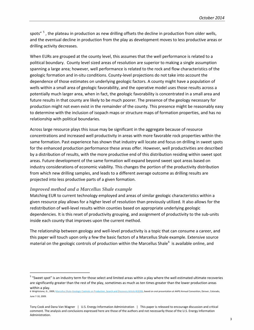
spots” 5 , the plateau in production as new drilling offsets the decline in production from older wells, and the eventual decline in production from the play as development moves to less productive areas or drilling activity decreases.

When EURs are grouped at the county level, this assumes that the well performance is related to a political boundary. County level sized areas of resolution are superior to making a single assumption spanning a large area; however, well performance is related to the rock and flow characteristics of the geologic formation and in-situ conditions. County-level projections do not take into account the dependence of those estimates on underlying geologic factors. A county might have a population of wells within a small area of geologic favorability, and the operative model uses those results across a potentially much larger area, when in fact, the geologic favorability is concentrated in a small area and future results in that county are likely to be much poorer. The presence of the geology necessary for production might not even exist in the remainder of the county. This presence might be reasonably easy to determine with the inclusion of isopach maps or structure maps of formation properties, and has no relationship with political boundaries.

Across large resource plays this issue may be significant in the aggregate because of resource concentrations and increased well productivity in areas with more favorable rock properties within the same formation. Past experience has shown that industry will locate and focus on drilling in sweet spots for the enhanced production performance these areas offer. However, well productivities are described by a distribution of results, with the more productive end of this distribution residing within sweet spot areas. Future development of the same formation will expand beyond sweet spot areas based on industry considerations of economic viability. This changes the portion of the productivity distribution from which new drilling samples, and leads to a different average outcome as drilling results are projected into less productive parts of a given formation.

Improved method and a Marcellus Shale example Matching EUR to current technology employed and areas of similar geologic characteristics within a given resource play allows for a higher level of resolution than previously utilized. It also allows for the redistribution of well-level results within counties based on appropriate underlying geologic dependencies. It is this reset of productivity grouping, and assignment of productivity to the sub-units inside each county that improves upon the current method.

The relationship between geology and well-level productivity is a topic that can consume a career, and this paper will touch upon only a few the basic factors of a Marcellus Shale example. Extensive source material on the geologic controls of production within the Marcellus Shale6 is available online, and

5 “Sweet spot” is an industry term for those select and limited areas within a play where the well estimated ultimate recoveries are significantly greater than the rest of the play, sometimes as much as ten times greater than the lower production areas within a play. 6 Wrightstone, G., 2009, Marcellus Shale-Geologic Controls on Production, Search and Discovery Article #10206, based on oral presentation at AAPG Annual Convention, Denver, Colorado,

June 7-10, 2009.

October 2014

Tony Cook and Dana Van Wagner | U.S. Energy Information Administration | This paper is released to encourage discussion and critical comment. The analysis and conclusions expressed here are those of the authors and not necessarily those of the U.S. Energy Information Administration.

4

within the scientific literature, but are not themselves the main focus of this work. More extensive work of a similar nature7 has already been completed for other formations.

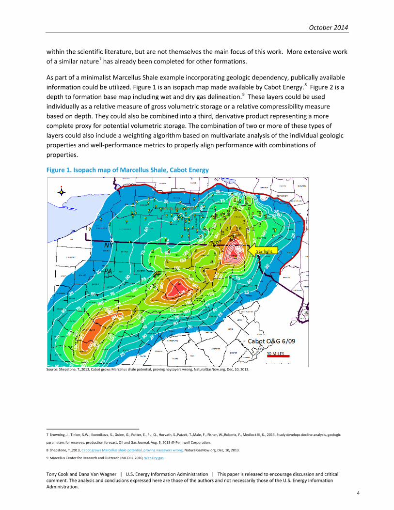
As part of a minimalist Marcellus Shale example incorporating geologic dependency, publically available information could be utilized. Figure 1 is an isopach map made available by Cabot Energy.8 Figure 2 is a depth to formation base map including wet and dry gas delineation.9 These layers could be used individually as a relative measure of gross volumetric storage or a relative compressibility measure based on depth. They could also be combined into a third, derivative product representing a more complete proxy for potential volumetric storage. The combination of two or more of these types of layers could also include a weighting algorithm based on multivariate analysis of the individual geologic properties and well-performance metrics to properly align performance with combinations of properties.

Figure 1. Isopach map of Marcellus Shale, Cabot Energy

Source: Shepstone, T.,2013, Cabot grows Marcellus shale potential, proving naysayers wrong, NaturalGasNow.org, Dec, 10, 2013.

7 Browning, J., Tinker, S.W., Ikonnikova, S., Gulen, G., Potter, E., Fu, Q., Horvath, S.,Patzek, T.,Male, F., Fisher, W.,Roberts, F., Medlock III, K., 2013, Study develops decline analysis, geologic

parameters for reserves, production forecast, Oil and Gas Journal, Aug. 5, 2013 @ Pennwell Corporation. 8 Shepstone, T.,2013, Cabot grows Marcellus shale potential, proving naysayers wrong, NaturalGasNow.org, Dec, 10, 2013. 9 Marcellus Center for Research and Outreach (MCOR), 2010, Wet-Dry gas.

October 2014

Tony Cook and Dana Van Wagner | U.S. Energy Information Administration | This paper is released to encourage discussion and critical comment. The analysis and conclusions expressed here are those of the authors and not necessarily those of the U.S. Energy Information Administration.

5

Figure 2. Depth of Marcellus Shale base and liquids/dry line (MCOR, 2010)

Source: Marcellus Center for Research and Outreach (MCOR), 2010, Wet-Dry gas.

These layers, and potentially many others, of the spatial distribution of formation properties across a play can be brought together in near endless combinations of intermediate products for model inputs. This paper will focus on demonstrating this method on the Marcellus Shale using a derivative product of geologic dependencies. Figure 3 is an overlay of the total extent of the formation across state boundaries. Inside the total extent of the formation is a colored overlay of gas in-place from Range Resources10 , with cooler colors representing less gas in-place and hotter colors more gas in-place. The overlay represents a given geographic information system (GIS) layer and is the initial input into the system.

10 Range Resources Corporation Company Presentation, 2013, p. 11.

October 2014

Tony Cook and Dana Van Wagner | U.S. Energy Information Administration | This paper is released to encourage discussion and critical comment. The analysis and conclusions expressed here are those of the authors and not necessarily those of the U.S. Energy Information Administration.

6

Figure 3. Marcellus Shale extent and Range Resources gas in-place outline

Source: U.S. Energy Information Administration based on information from a Range Resources Corporation Company Presentation, 2013

In this example a gas in-place GIS layer represents a derivative geologic dependency, specifically, gas storage capacity. However, a gas in-place calculation encompasses what otherwise would be several critical formation properties, such as gas filled porosity, net thickness, and reservoir pressure. If only the components of a gas storage layer were available, these could also be used together with a weighting function to build the necessary relationships between geology and well performance. Gas (or oil) in-place information has an additional value in terms of derivative products across many formations and is a primary layer of interest within this system of modeling. Figure 4 shows the Range Resources gas in-place contour map with current locations of Pennsylvanian Marcellus Shale wells used in the EIA EUR calculation. Different contours represent different estimates of gas in-place resource, and each of these contours can then be described in terms of its EUR performance.

October 2014

Tony Cook and Dana Van Wagner | U.S. Energy Information Administration | This paper is released to encourage discussion and critical comment. The analysis and conclusions expressed here are those of the authors and not necessarily those of the U.S. Energy Information Administration.

7

Figure 4. Gas In-Place Map Based on Range Resources, including Pennsylvania counties and well Locations

Source: U.S. Energy Information Administration based on information from a Range Resources Corporation Company Presentation, 2013

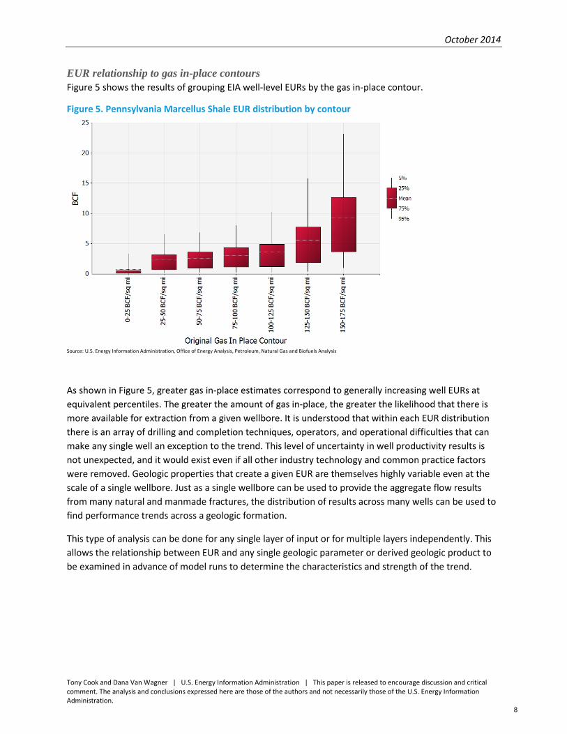
Well-level EURs were used as the performance measure basis for each contour. Horizontal well EURs with the minimum amount of information, as described previously, were grouped by contour to determine the range of performance in each contour. Figure 5 shows the EUR range and trend as gas in-place volumes increase by contour.

October 2014

Tony Cook and Dana Van Wagner | U.S. Energy Information Administration | This paper is released to encourage discussion and critical comment. The analysis and conclusions expressed here are those of the authors and not necessarily those of the U.S. Energy Information Administration.

8

EUR relationship to gas in-place contours Figure 5 shows the results of grouping EIA well-level EURs by the gas in-place contour.

Figure 5. Pennsylvania Marcellus Shale EUR distribution by contour

Source: U.S. Energy Information Administration, Office of Energy Analysis, Petroleum, Natural Gas and Biofuels Analysis

As shown in Figure 5, greater gas in-place estimates correspond to generally increasing well EURs at equivalent percentiles. The greater the amount of gas in-place, the greater the likelihood that there is more available for extraction from a given wellbore. It is understood that within each EUR distribution there is an array of drilling and completion techniques, operators, and operational difficulties that can make any single well an exception to the trend. This level of uncertainty in well productivity results is not unexpected, and it would exist even if all other industry technology and common practice factors were removed. Geologic properties that create a given EUR are themselves highly variable even at the scale of a single wellbore. Just as a single wellbore can be used to provide the aggregate flow results from many natural and manmade fractures, the distribution of results across many wells can be used to find performance trends across a geologic formation.

This type of analysis can be done for any single layer of input or for multiple layers independently. This allows the relationship between EUR and any single geologic parameter or derived geologic product to be examined in advance of model runs to determine the characteristics and strength of the trend.

October 2014

Tony Cook and Dana Van Wagner | U.S. Energy Information Administration | This paper is released to encourage discussion and critical comment. The analysis and conclusions expressed here are those of the authors and not necessarily those of the U.S. Energy Information Administration.

9

EUR and area relationship It has been noted for decades that the distribution of field sizes in conventional concentrations of hydrocarbons are highly skewed.11 Figure 5 demonstrates that well-level results within a tight or shale producing formation are also skewed distributions. The EUR distribution within each contour is skewed and distribution means progressively increase with resource concentration. Applying the area of each contour and the mean EUR for that contour allows the concentration of resource within a given area to be quantified.

The resulting summation of area and performance might best be described as a back of the envelope estimate of recoverable resource and should in no way be mistaken for a thorough or complete representation of economic or technically recoverable resource. Neither economic criteria, changes in recovery factor due to interfering well performance, nor exclusions due to access or policy concerns are included in this estimate. At best it is a simplistic example to show that resources are concentrated within smaller areas inside a given geologic unit.

Table 1. Estimates of EUR and area for Pennsylvania contour areas in the Marcellus Shale

Contour

(bcf/sq mi)

Area

(sq mi)

Average EUR

(bcf)

Resource Est.

(TCF)

Area

(%)

Resource

(%)

150-175 304.8 9.19 12.0 1.2 3.9

125-150 1408.3 5.59 33.8 5.3 10.9

100-125 1886.6 3.59 29.1 7.2 9.4

75-100 2,941.4 3.05 38.6 11.2 12.5

50-75 11798.7 2.55 129.4 44.8 41.8

25-50 6259.3 2.28 61.5 23.8 19.9

0-25 1734.2 0.68 5.1 6.6 1.6

Total-> 309.5 Source: U.S. Energy Information Administration, Office of Energy Analysis, Petroleum, Natural Gas and Biofuels Analysis

Based on the previously explained uncertainties in well EUR results, a more appropriate approach of potential resource estimation would incorporate the full range of EUR results. The process consists of multiplying each EUR distribution (without consideration for geologic failure at any well location) and assumed drainage area by the area of the contour and summing the results for all contours. The EUR distributions are assumed to be independent for this example, and the results are demonstrated in Figure 6. The results could also be interpreted as a recoverable resource estimate demonstrating the sensitivity of the estimate on the uncertainty of the EUR. Simple point estimates do not have the ability to quantify how fundamental uncertainties affect a final answer.

11 Arps, J.J., and Roberts, T.G., 1958, Economics of drilling for Cretaceous oil on east flank of Denver-Julesburg Basin: American Association of Petroleum Geologists Bulletin, v. 42, no. 11, p.

2549–2566.

October 2014

Tony Cook and Dana Van Wagner | U.S. Energy Information Administration | This paper is released to encourage discussion and critical comment. The analysis and conclusions expressed here are those of the authors and not necessarily those of the U.S. Energy Information Administration.

10

Figure 6. Wet natural gas resource estimate in the Marcellus Shale

Source: U.S. Energy Information Administration, Office of Energy Analysis, Petroleum, Natural Gas and Biofuels Analysis

In addition to uncertainties in well EURs (and additional geologic properties underlying flow rates such as permeability) that can affect a result, there is also a concentration of resources within the areas of superior storage capability. Table 1 indicates that the top three contours contain 13.7% of the area but 24.2% of the resource. Additional assumptions of well interference and the change in recovery factor that might come with them, particularly in the areas of higher resource concentration, would increase this concentration further still. Discussions on statistical measures of well performance under conditions of varied well interference conditions are discussed elsewhere.12 Also not included in this rough calculation of resource concentration would be the expectation of decreased geologic chance of success within the areas of less geologic storage. This effect would tend to increase the failure rate of wells in poorer areas of resource concentration, again attenuating the recoverability fraction of the better areas.

Change in county level EUR results Counties can easily contain one or more contours, each with a different range of EURs. Table 2 shows the difference between a simple average of well EURs at the county level and well EURs weighted by contour at the county level.

12 Cook, T.A., 2014, Oil and gas resource estimates and issues in tight and shale formations: modeling concepts, EIA working paper in review.

October 2014

Tony Cook and Dana Van Wagner | U.S. Energy Information Administration | This paper is released to encourage discussion and critical comment. The analysis and conclusions expressed here are those of the authors and not necessarily those of the U.S. Energy Information Administration.

11

Table 2. Pennsylvania Marcellus Shale EURs by county

PA County

Average EUR per county

(BCF)

Average EUR weighted to GIP contours within

county (BCF)

ALLEGHENY 3.74 4.09 ARMSTRONG 0.91 2.72 BEAVER 2.74 2.44 BEDFORD 1.16 0.85 BLAIR 1.34 1.23 BRADFORD 5.70 3.94 BUTLER 1.74 2.72 CAMBRIA 1.46 2.43 CAMERON 0.33 2.69 CENTRE 1.87 1.46 CLARION 1.24 2.55 CLEARFIELD 1.96 2.57 CLINTON 3.87 2.12 COLUMBIA 0.79 1.30 CRAWFORD 1.21 1.16 ELK 1.77 2.60 ERIE 1.21 0.35 FAYETTE 1.55 2.47 FOREST 1.58 2.55 GREENE 2.29 3.46 INDIANA 1.06 2.64 JEFFERSON 1.20 2.55 LACKAWANNA 1.25 1.32 LAWRENCE 1.28 1.77 LUZERNE 0.94 0.93 LYCOMING 3.74 2.57 MC KEAN 2.09 2.39 MERCER 1.28 1.22 MONTOUR 0.90 0.80 NORTHUMBERLAND 0.31 0.36 POTTER 1.77 2.50 SOMERSET 1.60 2.33 SULLIVAN 7.27 5.39 SUSQUEHANNA 6.14 4.92 TIOGA 2.98 2.49 UNION 2.80 0.30 VENANGO 0.83 2.49 WARREN 1.84 2.28 WASHINGTON 2.45 3.69 WAYNE 7.49 1.34 WESTMORELAND 1.85 2.84 WYOMING 8.85 3.42

Source: U.S. EIA Office of Energy Analysis, Petroleum, Natural Gas and Biofuels Analysis

October 2014

Tony Cook and Dana Van Wagner | U.S. Energy Information Administration | This paper is released to encourage discussion and critical comment. The analysis and conclusions expressed here are those of the authors and not necessarily those of the U.S. Energy Information Administration.

12

An examination of results for individual counties presented in Table 2 shows that some average EUR values changed in predictable ways. Wyoming County has several contours within it, and those contours are expected to have lower potential than the locations of the current drilling results. If only the highly productive and initially located and drilled areas are projected across the county, the result would be an overestimate based on a political boundary, rather than a lower estimate reflecting the change in an underlying geologic parameter and accompanying expected decrease in well performance. Central Pennsylvania counties such as Indiana and Jefferson more than double in expected well productivity because of the particular performance expected from the contours that underlie these counties. Even if that performance has not been achieved to date, it is reasonable to assume that as more wells are drilled, the results will reflect the contour they reside within rather than limited sampling of well productivity to date in any particular county or adjacent counties.

Additional benefits The preceding example is a demonstration of a single link between well productivities and geologic storage capacity. As additional geologic information is brought into this type of system, and more play-level analysis of this type is completed, a matrix relating geological criteria and well-level performance becomes a possible additional product. There is no restriction to the type or amount of geologic information that can be included and, with the addition of a weighting scheme, several parameters could be included rather than the single layer of gas storage demonstrated here.

As more information is accumulated across multiple plays or producing regions the possibility that additional relationships could be established is highly likely. In effect, the accumulation of multiple levels of well performance with multiple types of geologic parameters would allow for the creation of a matrix of geologic properties matched with well-performance parameters. At a later point in time this matrix of geologic properties could be matched to an area with similar geology but lacking well productivity. Even a moderate accumulation of well productivity and accompanying geologic dependency information has the potential to lead to a substantial improvement in modeling results in areas where current well productivity information is minimal.

Conclusions When projecting resource-to-production conversions spanning large periods of time it must be understood that the final answer will not be known until all drilling stops, the wells are depleted over decades, and every well is plugged and abandoned. Only then can the question of real-world productivity be answered with absolute certainty. Even then, however, there is the possibility that the answer could change in the future with a new cycle of development. The Devonian-aged shales of Ohio, West Virginia, and Pennsylvania have gone through previous cycles of development, and the recent activity in the Marcellus Shale formation is just a continuation of this pattern. With each new well drilled and wire-line log run, each barrel of oil or cubic foot of gas produced, each bit of information gathered, more is known, and this knowledge narrows the uncertainty in the geology, well results and future resource estimates.

Several potential methods of improvement have been discussed in this paper. Higher levels of modeling resolution, and higher levels of resolution directly tied to the physical properties of the rock that determines well productivity, allows for a better understanding of potential drilling locations and results. Production projections would be better oriented towards the same higher productivity geologic

October 2014

Tony Cook and Dana Van Wagner | U.S. Energy Information Administration | This paper is released to encourage discussion and critical comment. The analysis and conclusions expressed here are those of the authors and not necessarily those of the U.S. Energy Information Administration.

13

sweet spots that industry themselves recognize and seek out as initial drilling targets. Identifying the size, potential, and geologic conditions of these sweet spots is therefore of crucial importance to economic models attempting to mimic real-world behavior. While it is a characteristic of resource plays that nearly all sedimentary rock can produce some oil or gas, the likelihood of potential development lies within the formations and areas that are economically viable.