Working Paper Series - ecb.europa.eu · ator. The inclusion of an MA component generally improves...

Working Paper Series Mixed frequency models with MA components

Claudia Foroni, Massimiliano Marcellino, Dalibor Stevanović

Disclaimer: This paper should not be reported as representing the views of the European Central Bank (ECB). The views expressed are those of the authors and do not necessarily reflect those of the ECB.

No 2206 / November 2018

Abstract

Temporal aggregation in general introduces a moving average (MA) component in the

aggregated model. A similar feature emerges when not all but only a few variables are

aggregated, which generates a mixed frequency model. The MA component is generally

neglected, likely to preserve the possibility of OLS estimation, but the consequences have

never been properly studied in the mixed frequency context. In this paper, we show, analyt-

ically, in Monte Carlo simulations and in a forecasting application on U.S. macroeconomic

variables, the relevance of considering the MA component in mixed-frequency MIDAS and

Unrestricted-MIDAS models (MIDAS-ARMA and UMIDAS-ARMA). Specifically, the sim-

ulation results indicate that the short-term forecasting performance of MIDAS-ARMA and

UMIDAS-ARMA is better than that of, respectively, MIDAS and UMIDAS. The empirical

applications on nowcasting U.S. GDP growth, investment growth and GDP deflator inflation

confirm this ranking. Moreover, in both simulation and empirical results, MIDAS-ARMA is

better than UMIDAS-ARMA.

Keywords: Temporal aggregation, MIDAS models, ARMA models.

JEL Classification Code: E37, C53.

ECB Working Paper Series No 2206 / November 2018 1

Non-technical summary

Temporal aggregation generally introduces a moving average (MA) component in the model

for the aggregate variable. A similar feature should be present in the mixed frequency models,

and indeed we show formally that this is in general the case. The effects of neglecting the

MA component have been rarely explicitly considered in a single frequency context. For mixed

frequency models, there are no results available.

We close this gap and analyze the relevance of the inclusion of an MA component in mixed-data

sampling (MIDAS) and unrestricted mixed-data sampling (UMIDAS) models, with the resulting

specifications labeled, respectively, MIDAS-ARMA and UMIDAS-ARMA. We first compare the

forecasting performance of the mixed frequency models with and without the MA component in

a set of Monte Carlo experiments, using a variety of Data Generating Processes (DGPs). Next,

we carry out an empirical investigation, where we predict several quarterly macroeconomic

variables using timely monthly indicators. In particular, we forecast three relevant quarterly

U.S. macroeconomic variables: real GDP growth, real private non residential fixed investment

(PNFI) growth and GDP deflator inflation.

In the Monte Carlo simulations, the short-term forecasting performance is better when in-

cluding the MA component, and the gains are higher the more persistent is the series. Moreover,

in general the MIDAS-ARMA specifications are slightly better than the UMIDAS-ARMA spec-

ifications. This pattern suggests that adding the MA component to the MIDAS model helps

somewhat in reducing the potential misspecification due to imposing a specific lag polynomial

structure. In the empirical exercise, the inclusion of an MA component generally improves the

forecasting performance substantially. For all variables, and in line with the simulation results,

MIDAS-ARMA is better than UMIDAS-ARMA.


1 Introduction

The use of mixed-frequency models has become increasingly popular among academics and

practitioners. It is in fact by now well recognized that a good nowcast or short-term forecast

for a low frequency variable, such as GDP growth and its components, requires to exploit the

timely information contained in higher frequency macroeconomic or financial indicators, such

as surveys or spreads. A growing literature has flourished proposing different methods to deal

with the mixed-frequency feature. In particular, models cast in state-space form, such as vector

autoregressions (VAR) and factor models, can deal with mixed-frequency data, taking advantage

of the Kalman filter to interpolate the missing observations of the series only available at low

frequency (see, among many others, Mariano and Murasawa (2010) and Giannone et al. (2008)

in a classical context, and Eraker et al. (2015) and Schorfheide and Song (2015) in a Bayesian

context). A second approach has been proposed by Ghysels (2016). He introduces a different

class of mixed-frequency VAR models, in which the vector of endogenous variables includes

both high and low frequency variables, with the former stacked according to the timing of the

data releases. A third approach is the mixed-data sampling (MIDAS) regression, introduced by

Ghysels et al. (2006), and its unrestricted version (UMIDAS) by Foroni et al. (2015). MIDAS

models are tightly parameterized, parsimonious models, which allow for the inclusion of many

lags of the explanatory variables. Given their non-linear form, MIDAS models are typically

estimated by non-linear least squares (NLS)1. UMIDAS models are the unrestricted counterpart

of MIDAS models, which can be estimated by simple ordinary least squares (OLS), but work

well only when the frequency mismatch is small.2

In this paper, we start from the observation that temporal aggregation generally introduces a

moving average (MA) component in the model for the aggregate variable (see, e.g., Marcellino

(1999) and the references therein). A similar feature should be present in the mixed frequency

models, and indeed we show formally that this is in general the case3. The MA component is

often neglected, both in same frequency and in mixed frequency models, likely to preserve the

1In a recent paper Ghysels and Qian (2018) propose to use OLS estimation of the MIDAS regression slope andintercept combined with profiling the polynomial weighting scheme parameters.

2The literature on mixed-frequency approaches is vast. The papers cited in the text are a non-exhaustive listof key contributions to the field. For a review of the mixed-frequency literature, see Bai et al. (2013) and Foroniand Marcellino (2013) among many others.

3An analysis of identifiability on ARMA processes with mixed-frequency observations is provided by Andersonet al. (2016), on VARMA processes by Deistler et al. (2017).


possibility of OLS estimation and on the grounds that it can be approximated by a sufficiently

long autoregressive (AR) component.

The effects of neglecting the MA component have been rarely explicitly considered. In a single

frequency context, Lutkepohl (2006) showed that VARMA models are especially appropriate

in forecasting, since they can capture the dynamic relations between time series with a small

number of parameters. Further, Dufour and Stevanovic (2013) showed that a VARMA instead of

VAR model for the factors provides better forecasts for several key macroeconomic aggregates

relative to standard factor models, as well as producing a more precise representation of the

effects and transmission of monetary policy. Leroux et al. (2017) found that ARMA(1,1) models

predict well the inflation change and outperform many data-rich models, confirming the evidence

on forecasting inflation by Stock and Watson (2007), Faust and Wright (2013) and Marcellino

et al. (2006). Finally, VARMA models are often the correct reduced form representation of

DSGE models (see, for example, Ravenna (2007)). For mixed frequency models, there are no

results available.

We close this gap and analyze the relevance of the inclusion of an MA component in MIDAS

and UMIDAS models, with the resulting specifications labeled, respectively, MIDAS-ARMA and

UMIDAS-ARMA. We first compare the forecasting performance of the mixed frequency models

with and without the MA component in a set of Monte Carlo experiments, using a variety of

Data Generating Processes (DGPs). It turns out that the short-term forecasting performance

is better when including the MA component, and the gains are higher the more persistent is

the series. Moreover, in general the MIDAS-ARMA specifications are slightly better than the

UMIDAS-ARMA specifications, though the differences are minor. This pattern is in contrast

with the findings in Foroni et al. (2015), and suggests that adding the MA component to the

MIDAS model helps somewhat in reducing the potential misspecification due to imposing a

specific lag polynomial structure.

Next, we carry out an empirical investigation, where we predict several quarterly macroe-

conomic variables using timely monthly indicators. In particular, we forecast three relevant

quarterly U.S. macroeconomic variables: real GDP growth, real private non residential fixed

investment (PNFI) growth and GDP deflator inflation. The latter variable is particularly rele-

vant, as Stock and Watson (2007) show that the MA component for US inflation is important,

especially after 1984. In fact, while during the 1970s the inflation process could be very well


approximated by a low order AR, after the 1980s this has become less accurate and the inclusion

of an MA component more relevant. Evidence on the importance of the MA component for the

U.S. inflation is also found by Ng and Perron (2001) and Perron and Ng (1996). As monthly ex-

planatory variables, we consider industrial production and employment for the real GDP growth

and the PNFI growth, CPI inflation and personal consumption expenditures (PCE) inflation

for the GDP deflator. The inclusion of an MA component generally improves the forecasting

performance substantially. In particular, adding the MA part to forecast GDP growth one-year

ahead ameliorates the MSE up to 10%, while for PNFI we obtain even bigger gains, up to 30%

one-year ahead. Also in the case of GDP deflator we obtain robust improvements, which go up

to 15%. For all variables, and in line with the simulation results, MIDAS-ARMA is better that

UMIDAS-ARMA. Lastly, full sample estimates of MA coefficients are significant and important

in most of MIDAS-ARMA and UMIDAS-ARMA specifications.

The remainder of the paper proceeds as follows. In Section 2 we show that temporal aggre-

gation generally creates an MA component also in mixed frequency models. In Section 3 we

describe parameter estimators for the MIDAS-ARMA and UMIDAS-ARMA models. In Section

4 we present the design and results of the simulation exercises. In Section 5 we develop the em-

pirical applications on forecasting U.S. quarterly variables with monthly indicators. In Section 6

we summarize main results and conclude. Robustness analysis on the Monte Carlo simulations

and the empirical applications are reported in Appendix.

2 The rationale for an MA component in mixed frequency mod-

els

The UMIDAS regression approach can be derived by aggregation of a general dynamic linear

model in high frequency, as shown by Foroni et al. (2015), while the MIDAS model imposes

specific restrictions on the UMIDAS coefficients in order to reduce their number, which is par-

ticularly relevant when the frequency mismatch is large (for example, with daily and quarterly

series). In Section 2.1, we briefly review the derivation of the UMIDAS model, highlighting

that, in general, there should be an MA component, even though it is generally disregarded. In

Section 2.2, we provide two simple analytical examples in which, starting from a high-frequency


model without MA term, we end up with a mixed frequency model in which the MA compo-

nent is present. We discuss estimation of mixed frequency models with an MA component in a

separate section.

2.1 UMIDAS regressions and dynamic linear models

Let us assume that the Data Generating Process (DGP) for the variable y and the N variables

x is an ARDL(p, q) process, as in Foroni et al. (2015):

a(L)ytm = b1(L)x1tm + ...+ bN (L)xNtm + eytm (1)

where a(L) = 1 − a1L − ... − apL, bj(L) = bj1L + ... + bjqLq, j = 1, ..., N , and the error eytm

is white noise. We assume, for simplicity, that p = q and the starting values y−p, ..., y0 and

x−p, ..., x0 are all fixed and equal to zero.

We then assume that x can be observed for each period tm, while y can be only observed

every m periods. We define t = 1, ..., T as the low frequency (LF) time unit and tm = 1, ..., Tm

as the high frequency (HF) time unit. The HF time unit is observed m times in the LF time

unit. As an example, if we are working with quarterly (LF) and monthly (HF) data, it is m = 3

(i.e., three months in a quarter). Moreover, L indicates the lag operator at tm frequency, while

Lm is the lag operator at t frequency.

We also introduce the aggregation operator

ω(L) = ω0 + ω1L+ ...+ ωm−1Lm−1, (2)

which characterizes the temporal aggregation scheme. For example, ω(L) = 1 + L+ ...+ Lm−1

indicates the sum of the high-frequency observations over the low-frequency period, typically

used in the case of flow variables, while ω(L) = 1 corresponds to point-in-time sampling and is

typically used for stock variables. As we will see, different aggregation schemes will play a role

in generating MA components.

To derive the generating mechanism for y at mixed frequency (MF), we introduce a polynomial

in the lag operator, β(L), whose degree in L is at most equal to pm− p and which is such that

the product h(L) = β(L)a(L) only contains powers of Lm. This means that h(L) is a polynomial


of the form h0L0 + h1L

m + h2L2m + ...+ hpm−pL

pm−p. It can be shown that such a polynomial

always exists, and its coefficients depend on those of a(L), see Marcellino (1999) for details.

In order to determine the AR component of the MF process, we then multiply both sides of

(1) by ω(L) and β(L) to get

h(L)ω(L)ytm = β(L)b1(L)ω(L)x1tm + ...+ β(L)bN (L)ω(L)xNtm + β(L)ω(L)eytm . (3)

Hence, the autoregressive component only depends on LF values of y. Let us consider now

the x variables, which are observable at high frequency tm. Each HF xitm influences the LF

variable y via a polynomial β(L)bj(L)ω(L) = bj(L)β(L)ω(L), j = 1, ..., N . We see that it is a

particular combination of high-frequency values of xj , equal to β(L)ω(L)xjtm , that affects the

low-frequency values of y.

Only under certain, rather strict conditions, it is possible to recover the polynomials a(L) and

bj(L) that appear in the HF model for y from the MF model, and in these cases also β(L) can

be identified. Therefore, when β(L) cannot be identified, we can estimate a model as

c(Lm)ω(L)ytm = δ1(L)x1tm−1 + ...+ δN (L)xNtm−1 + εtm , (4)

tm = m, 2m, 3m, ...

where c(Lm) = (1− c1Lm − ...− ccLmc), δj(L) = (δj,0 + δj,1L+ ...+ δj,vLv), j = 1, ..., N .

We can focus now on the error term of equation (3). In general, there is an MA component in

the MF model, q(Lm)uytm , with q(Lm) = (1+q1Lm+...+qqL

mq). The order of q(Lm), q, coincides

with the highest multiple of m non zero lag in the autocovariance function of β(L)ω(L)eytm .

The coefficients of the MA component have to be such that the implied autocovariances of

q(Lm)uytm coincide with those of β(L)ω(L)eytm evaluated at all multiples of m. Consequently,

also the error term εtm in the approximate mixed frequency model (4), which is the UMIDAS

model, in general has an MA structure. It can be shown that the maximum order of the MA

structure is p for average sampling and p-1 for point-in-time sampling, where p is the order

of the AR component in the high frequency model for ytm (see, e.g., Marcellino (1999) for a

derivation of this results)4.

4The fact that an aggregated model is misspecified and leads to biased and inconsistent estimators has beenhighlighted by Andreou et al. (2010). However, contrary to us, they do not focus on the presence of an MAcomponent in the aggregation.


2.2 Two analytical examples

In this section, we consider two simple DGPs and show that, even in these basic cases, an

MA component appears in the mixed frequency model. In the first example, we consider an

ARDL(1,1) with average sampling, in the second one an ARDL(2,2) with point-in-time sampling.

In both cases, we work with monthly and quarterly variables, therefore m = 3, as in the empirical

applications that will be presented later on. The examples could be easily generalized to consider

higher order models and different frequency mismatches m.

ARDL(1,1) with average sampling

Let us assume an ARDL(1,1) as HF DGP:

ytm = aytm−1 + bxtm−1 + eytm , (5)

where ytm is a variable unobservable at HF, xtm is the high-frequency variable, eytm is white

noise, and tm is the high-frequency time index. Although we do not observe ytm , we observe the

quarterly aggregated values of the series.

In order to obtain the model for the quarterly aggregated series, let us write (5) as

(1− aL) ytm = bLxtm + eytm . (6)

We consider average sampling, and therefore we define the aggregation operator ω (L) = 1 +

L+ L2. Then, we first introduce a polynomial in the lag operator, β(L), which is such that the

product h(L) = β(L) (1− aL) only contains powers of L3. This polynomial exists and it is equal

to(1 + aL+ a2L2

). We then multiply both sides of equation (6) by ω (L) and β (L) and we

obtain:

(1 + aL+ a2L2

)(1− aL)

(1 + L+ L2

)ytm =

(1 + aL+ a2L2

)bL(1 + L+ L2

)xtm +(

1 + aL+ a2L2) (

1 + L+ L2)eytm , (7)

or equivalently:

(1− a3L3

)ytm =

(1 + aL+ a2L2

)bL(1 + L+ L2

)xtm +(

1 + (a+ 1)L+(a2 + a+ 1

)L2 +

(a2 + a

)L3 + a2L4

)eytm , (8)


where ytm =(1 + L+ L2

)ytm and tm = 3, 6, 9, ... .

As we saw it in Section 2.1, the order of the MA component coincides with the highest

multiple of 3 non zero lag in the autocovariance function of the error term in equation (8), and

it is bounded above by the AR order of the model for ytm .

Eq. (8) is then estimated at quarterly frequency, but making use of all the information

available in the HF variable xtm , and including the MA component, which is of order 1 in this

case (being the relevant lag for the quarterly model L3). The model in eq. (8) is therefore a

UMIDAS-AR with an MA(1) component.

ARDL(2,2) with point-in-time sampling

Let us now assume an ARDL(2,2) as HF DGP:

ytm = a1ytm−1 + a2ytm−2 + b1xtm−1 + b2xtm−2 + eytm , (9)

or, equivalently, (1− a1L− a2L2

)ytm =

(b1L+ b2L

2)xtm + eytm , (10)

where ytm , xtm , eytm and tm are defined as in the previous example.

We consider point-in-time sampling, and therefore ω (L) = 1. Next, we need to multiply

both sides of equation (9) by ω(L) and find a polynomial β(L) such that the product h(L) =

β(L)(1− a1L− a2L2

)only contains powers of L3. In can be easily shown that β (L) exists and

it is equal to (1 + a1L+

(a21 + a2

)L2 − a1a2L3 + a22L

4).

The resulting mixed frequency model for the low-frequency variable is:

(1−

(a31 + 3a2a1

)L3 − a32L6

)ytm =

(1 + a1L+

(a21 + a2

)L2 − a1a2L3 + a22L

4) (b1L+ b2L

2)xtm +(

1 + a1L+(a21 + a2

)L2 − a1a2L3 + a22L

4)eytm , (11)

with tm = 3, 6, 9, ... Hence, also in this case there is an MA component in the mixed frequency

model for y. Its order coincides with the highest multiple of 3 non zero lag in the autocovariance

function of(1 + a1L+

(a21 + a2

)L2 − a1a2L3 + a22L

4)eytm , and it is bounded above by the AR

order of the model for ytm minus one, which is 1 in this example. Following the same line of

reasoning as in the previous example, the MA component is of order 1.


3 UMIDAS-ARMA and MIDAS-ARMA: forecasting specifica-

tions and estimation

We describe now in more detail the model specifications we consider for forecasting, and

the estimation details. We first recall the main features of the standard MIDAS regression,

introduced by Ghysels et al. (2006), and its unrestricted version, as in Foroni et al. (2015).

Then, we discuss their extensions to allow for an MA component and we discuss the estimation

of the models.

The starting point for our MF models is equation (4). In order to simplify the notation, we

assume ω(L) = 1 and one explanatory variable xtm5. Further, we allow for incorporating leads

of the high frequency variable in the projections, which captures asynchronous releases.

The equation we are going to estimate to generate an hm-step ahead forecast is the following:

ytm = c(Lm)ytm−hm + δ(L)xtm−hm+w + εtm , (12)

where c(Lm) is a modified lag structure of equation (4) to obtain a direct forecast and w is the

number of months with which x is leading y.

If εtm is serially uncorrelated, equation (12) represents the UMIDAS-AR model. Given that

the model is linear, the UMIDAS-AR regression can be estimated by simple OLS. Empirically,

the lag length of the high frequency variable x is often selected by means of an information

criterion, such as the BIC.

Adding an MA component to the UMIDAS-AR yields the UMIDAS-ARMA model:

ytm = c(Lm)ytm−hm + δ(L)xtm−hm+w + utm + q(Lm)utm−hm , (13)

where utm is a (weak) white noise with E(utm) = 0 and E(utmu′tm) = σ2u < ∞, and all the

remaining terms stay the same as in equation (12). Given that MIDAS models are direct

forecasting tools, we decided to follow a direct approach also when modelling the MA component.

Note that if equation (4) coincides with the DGP, then the errors in equation (12) will be serially

correlated. This provides an additional justification for the use of MA errors.

5This is an innocuous simplification, as with a generic aggregation scheme ω(L) 6= 1 we could just work withthe redefined variable ytm = ω(L)ytm .


OLS estimation of the UMIDAS-ARMA model is no longer possible, because of the MA

component in the residuals. We then estimate the model as in the standard ARMA literature,

by maximum likelihood or, as we will actually do to be coherent with the MIDAS literature, by

non-linear least squares (NLS).

The MIDAS-AR specification is a restricted version of the UMIDAS-AR. The MIDAS-AR

model as in Ghysels et al. (2006), specified for forecasting hm periods ahead, can be written as

follows:

ytm = c(Lm)ytm−hm + βB(L, θ)xtm−hm+w + εtm , (14)

where

B(L, θ) =K∑j=0

b(j, θ)Lj ,

b(j, θ) =exp(θ1j + θ2j

2)∑Kj=0 exp(θ1j + θ2j2)

,

and K is the maximum number of lags included of the explanatory variable.

As it is clear by comparing equation (12) and equation (14), the MIDAS model is nested into

the UMIDAS model.

The MIDAS-AR model in equation (14) is estimated by NLS. Given that it is hm-dependent,

as in the UMIDAS case it has to be re-estimated for each forecast horizon.

Exactly as for the UMIDAS, we extend the MIDAS-AR in equation (14) to incorporate an

MA component:

ytm = c(Lm)ytm−hm + βB(L, θ)xtm−hm+w + utm + q(Lm)utm−hm , (15)

where the error term is defined as in (13). Given the nonlinearity of the model, we estimate its

parameters by NLS. Appendix A provides additional details on the NLS estimation procedures.

To conclude, it is worth briefly comparing the use for forecasting of UMIDAS-ARMA versus

the Kalman filter. The latter is clearly optimal in the presence of mixed frequency data and linear

models. However, UMIDAS-ARMA is equivalent if it is theoretically derived from a known high

frequency linear dynamic model, as UMIDAS-ARMA coincides with the mixed frequency data

generating process. The ranking of the two approaches is unclear if the high frequency model


is mis-specified. Moreover, the Kalman filter can incur into computational problems when the

frequency mismatch is large. Something similar happens to UMIDAS-ARMA, due to parameter

proliferation, and in this case the parsimony of MIDAS-ARMA can be particularly helpful. Bai

et al. (2013) propose a more detailed comparison of the Kalman filter and the MIDAS approach.

4 Monte Carlo evaluation

We now assess the forecasting relevance of including an MA component in MIDAS and UMI-

DAS models by means of simulation experiments. We use two designs, closely related to the

two analytical examples described in Section 2.2. We present first the Monte Carlo designs and

then the results. Finally, we summarize the results obtained from other variations of the Monte

Carlo design, aimed at making the evidence more robust. The detailed robustness checks are

presented in Appendix B.

4.1 Monte Carlo design

In the first design, the DGP is the HF ARDL(1,1):

ytm = ρytm−1 + δlxtm−1 + ey,tm , (16)

where ytm is unobservable at HF, but available at LF, while xtm is the HF variable, tm is the

HF time index, the aggregation frequency is m = 3 (as in the case of quarterly and monthly

frequencies), and t is the LF time index, with t = 3tm. We assume that ω(L) = 1 + L + L2,

corresponding to average sampling.

The shocks ey,tm are independent and sampled from a normal distribution. The variance of x

and that of the error ey,tm are set in such a way that the R2 in the model for y is equal to 0.9 in

each simulation. We consider different combinations of ρ and δl, representing different degrees

of persistence and correlation between the HF and the LF variables. In detail, we evaluate the

following parameter sets:

(ρ, δl) = {(0.1, 0.1) , (0.5, 0.1) , (0.9, 1) , (0.94, 1)} , (17)


and we would expect theoretically the relative importance of the MA component to increase

with the value of ρ.

Finally, xtm is generated as an AR(1) with coefficient ρ. We highlight that there is no need

to play on the persistence of xtm to obtain high or low R2, but we can obtain the same results

by changing the variance of the extm, and consequently of xtm .

In the second design, the DGP is the HF ARDL(2,2):

ytm = ρ1ytm−1 + ρ2ytm−2 + δl1xtm−1 + δl2xtm−2 + ey,tm . (18)

We still assume m = 3 but now ω(L) = 1, so that the LF variable is skip-sampled every m = 3

observations.

In this second DGP, we consider the following parameter combinations:

(ρ1, ρ2, δl1, δl2) = {(0.05, 0.1, 0.5, 1) , (0.125, 0.5, 0.125, 0.5) , (0.25, 0.5, 0.5, 1)} . (19)

All the other design features are as in the first DGP.

We focus on typical sample sizes for the estimation sample, with T = 50, 100. The size of the

evaluation sample is set to 50, and the estimation sample is recursively expanded as we progress

in the recursive forecasting exercise. The number of replications is 500.

The competing forecasting models are the following:

1. A MIDAS-AR model, with 12 lags in the exogenous HF variable and 1 lag in the AR

component;

2. A MIDAS-ARMA model, as in the previous point but with the addition of an MA com-

ponent;

3. A MIDAS-ARMA model, with only 3 lags in the exogenous HF variable and 1 AR lag;

4. A UMIDAS-AR model, with lag length selected according to the BIC criterion, where the

maximum lag length is set equal to 12;

5. A UMIDAS-ARMA model, as in the previous point, with the addition of an MA compo-

nent;


6. A UMIDAS-ARMA, fixing at 3 the number of lags of the HF exogenous variable.

In all ARMA models there is an MA(1) component, in line with the theoretical results, but an

higher order can be allowed. Further, a higher number of lags in the autoregressive component

can also be included.6

We evaluate the competing one-step ahead forecasts on the basis of their associated mean

square prediction error (MSE), assuming that information on the first two months of the quarter

is available (as it is common in nowcasting exercises).

4.2 Results

In Tables 1 to 4 we report the mean relative MSE across simulations, and numbers smaller

than one indicate that the model is better than the benchmark (model 1, the MIDAS-AR). We

also report the 10th, 25th, 50th, 75th and 90th percentiles, to provide a measure of the dispersion

in the results.

Tables 1 and 2 present the results for the first DGP (the ARDL(1,1) with average sampling),

using T = 100 in Table 1 and T = 50 in Table 2. The corresponding Tables 3 and 4 are based

on the second DGP (the ARDL(2,2) with point-in-time sampling).

A few key findings emerge. First, adding an MA component to the MIDAS model generally

helps. The gains are not very large but they are visible at all percentiles, with a few exceptions

for the second DGP. The gains are larger either with substantial persistence (ρ = 0.9 or ρ = 0.94

in the first DGP and ρ1 = 0.25, ρ2 = 0.5 in the second DGP) or with low persistence in the first

DGP (ρ = 0.1), but in the latter case the result is mainly due to a deterioration in the absolute

performance of the standard MIDAS model. The more parsimonious specification with 3 lags

only of the HF variable is generally better, except when ρ = 0.5.

Second, adding an MA component to the UMIDAS model is also generally helpful, though

the gains remain small.

Third, in general the MIDAS-ARMA specifications are slightly better than the UMIDAS-

ARMA specifications, though the differences are minor. This pattern is in contrast with the

6We computed results with 3 lags in the MIDAS-AR and UMIDAS-AR, to check whether inserting more lags inthe AR part serves as a proxy for the MA component. However, the relevance of the MA component is confirmed.Results are available upon request.


findings in Foroni et al. (2015), and suggests that adding the MA component to the MIDAS

model helps somewhat in reducing the potential misspecification due to imposing a specific lag

polynomial structure.

Finally, results are consistent across sample sizes, and the models do not seem sensitive to

short sample sizes.

4.3 Robustness checks

We run a battery of robustness checks on our Monte Carlo experiments, with the scope to

strengthen the evidence emerging from our main results. For the sake of conciseness, here we

report a summary of the checks and the main conclusions. The detailed results are presented in

Appendix B.

As a first robustness exercise, we modify the set up by reducing the explanatory power of the

x variable in such a way that the total R2 in our DGP for y is equal to 0.3, 0.5 or 0.7. The MSE

are obviously bigger in absolute value, but the MA component is still generally improving the

forecasting performance of the (U)MIDAS models. Second, we compute the results for a longer

estimation sample, with Tq = 200, which corresponds to 50 years of quarterly observations, in

line for example with empirical applications using long macroeconomic time series for the US.

The results show broadly the same features as when T = 100.

Finally, we consider not only nowcasting, but also 2- and 4-quarter ahead forecasts. Results

are overall robust at the 2-quarter ahead horizon, while at the 4-quarter ahead results are much

weaker. Theoretically, the relevance of the MA component should decline at longer horizons.

Indeed, the Monte Carlo results show smaller gains from the use of an MA component for

2-quarter ahead forecasting, and no gains at 4-quarter horizon.

5 Empirical applications

Applications of MIDAS regressions to forecasting macroeconomic variables is fairly standard

by now, starting from the paper by Clements and Galvo (2008) 7. Our focus is on the inclusion of

an MA component. Therefore, in this section, we look at the performance of our MA augmented

7Other studies which consider MIDAS applications are, among many others, Schumacher (2016) and Kim andSwanson (2017). For a comprehensive review, see Foroni and Marcellino (2013).


mixed frequency models in forecasting exercises with actual data. The analysis focuses on

forecasting quarterly U.S. variables.

In particular, we consider three relevant quarterly U.S. macroeconomic variables: real GDP

growth, real private non residential fixed investment (PNFI) growth and GDP deflator inflation.

As monthly explanatory variables, we consider industrial production and employment for the real

GDP growth and the PNFI growth, while we consider CPI inflation and personal consumption

inflation for the GDP deflator. A complete description of data sources and transformations is

available in Table 5.

The total sample spans over 50 years of data, from the first quarter of 1960 to the end of

2015. The forecasts are computed in pseudo real time, with progressively expanding samples.

The evaluation period goes from 1980Q1 to the end of the sample, covering roughly 35 years. At

each point in time, we compute forecasts from 1- up to 4-quarter ahead. The forecasting target

is the annualized growth rate. Although the information contained in the monthly variables

updates every month, we focus on the case in which the first two months of the quarter are

already available.

We consider the models (1) to (7) as described in Section 4.1, plus a simple low frequency

AR(1) model as a further benchmark for the usefulness of the mixed-frequency data8. In par-

ticular, we consider the direct forecast resulting from the model:

yt = c+ ρyt−h + et. (20)

We evaluate the forecasts both in terms of mean squared errors (MSE) and in terms of mean

absolute errors (MAE). We then compare the forecasting performance relative to a standard

MIDAS model with an autoregressive component and 12 lags of the explanatory variable (as the

model (1) in Section 4).

In Tables 6 to 8 we report the results for, respectively, the real GDP growth, the real PNFI

growth and the GDP deflator inflation rate. Each table is organized in the same way: it reports

the value of MSE and MAE for each model, the ratio of those criteria for each model relative to

the MIDAS-AR, our benchmark model, and the p-value of the Diebold-Mariano test, to check

8Despite for a variable like inflation more accurate benchmarks could be chosen, we consider an AR process,which is nested in all the models under comparison, and we keep it the same for all the variables under analysisto test the usefulness of mixed frequency data.


the statistical significance of the differences in forecast measures with respect to the benchmark

(see Diebold and Mariano (1995)).

The tables are broadly supportive of the inclusion of the MA component in the mixed fre-

quency models, as the MSE and MAE ratios are often smaller than one for the MIDAS-ARMA

and UMIDAS-ARMA models when compared with their versions without MA.9 More in detail:

for forecasting GDP growth, adding the MA component does not provide substantial improve-

ments with respect to standard mixed frequency models for h = 1, with industrial production

being the best indicator. When h = 2, employment becomes better than industrial production,

and adding an MA term matters, with gains of 8% for the MIDAS-ARMA model. A similar

results holds for h = 3, with gains increasing to 20%. Four-quarter ahead, industrial production

returns best, and MIDAS-ARMA leads to a decrease of 10% in the MSE. For PNFI growth,

MIDAS-ARMA is best at all horizons, with employment preferred to industrial production ex-

cept for h = 1. The gains are small for h = 1, 2, 3, in the range 1%-8%, but increase to 30% for

h = 4. For GDP deflator, PCE inflation is systematically better than CPI, and MIDAS-ARMA

yields gains for h = 1 and 2 of, respectively, 15% and 10%. It is also worth mentioning that MSE

and MAE lead to the same rankings, and that the gains from adding the MA parts are generally

statistically significant. Finally, the models perform well with respect to the AR benchmark.

Confirming the widespread evidence in the literature, the mixed frequency models perform the

best at short horizons. However, we get satisfactory results also up to h = 4.

The empirical gains resulting from the use of the MA term in the mixed frequency models

are somewhat larger than those in the Monte Carlo experiments. A possible reason is model

mis-specification, and in particular some form of parameter instability. In that case, the use of

an MA component can be helpful to put the forecasts ”back on track”, see for example Clements

and Hendry (1998) for details.

We now decompose the MSE in bias and variance, as:

MSE = (E(e))2︸︷︷︸Bias

+V ar(e)︸︷︷︸Variance

(21)

with e = y−y. We find that the MA part helps especially in reducing the bias, suggesting that the

MA part is important to well approximate the conditional mean of y (the optimal forecast under

9The models which include an MA component are indicated in bold in the tables, while the lowest MSE andMAE values are underlined.


the quadratic loss). When the models with the MA component are not performing well, this is

due especially to the variance term, instead. Detailed results on the bias/variance decomposition

are presented in Table 9. In particular, in the table we report the ratio of the bias and of the

variance of each model relative to the bias and variance of the MIDAS-AR model, which is taken

as a benchmark.

The MSE and MAE are computed over the entire evaluation sample. To check whether the

performance of our models remains good across the entire sample, in Figure 1 we report the one-

quarter ahead forecasts of the benchmark MIDAS-AR model and of one of the MA augmented

models, together with the realized series. In Figure 2, instead, we report the 4-quarter ahead

forecasts.10 It turns out that, on average, MIDAS models perform well throughout the sample,

both with and without an MA component.

Tables 10 and 11 report the full-sample estimates of MA coefficients in MIDAS-ARMA and

UMIDAS-ARMA models that have been used in the forecasting exercise. The corresponding

t-statistics are shown in parentheses. We observe that many MA coefficients are significant. For

instance, MA(1) coefficient in MIDAS-ARMA-3lags model on GDP growth equation with em-

ployment growth is precisely estimated at horizons h = 1, 2, 3. This MIDAS-ARMA model was

also the best in out-of-sample forecasting exercise, see table 6. In case of PNFI, when forecasting

one quarter ahead with industrial production as high frequency predictor, MA coefficient is sig-

nificant in all models. Same result holds at longer horizons with employment growth. When it

comes to GDP deflator prediction, an interesting finding is that the MA(2) component is highly

strong and significant for most of the horizons and models.

In Appendix C, we expand the empirical exercise along several dimensions. First, we analyse

a shorter sample ending in 2007Q3, to assess the effects of the recent crisis. Second, we report

results for the cases in which only one of the months of the quarters are available and when

instead all three months are already available. Third, we use a real-time dataset with the

different vintages.11

All in all, the robustness exercises confirm the evidence we find in this section. Excluding the

crisis, results do not change substantially, and remain broadly supportive of the inclusion of the

10Figures 1 and 2 focus only on a small portion of results that we have available. The same figures for othermodels, other forecast horizons and other explanatory variables are available upon request.

11As in the Monte Carlo, we could extend the number of lags in the AR component. However, we keep ourbenchmark specification of one AR lag, consistent with most of the empirical studies involving MIDAS. Resultswith 4 lags are available upon request.


MA component in the mixed-frequency models. In most of the cases, the best performing model

up to 2007 remains the best in the full sample. The magnitude of improvements is also very

comparable. For the other nowcasting horizons (that is, including only one month of monthly

information or, instead, all the three months), results confirm that in most of the cases the best

performance is obtained when the MA component is added. Finally, when using real-time data

for the macroeconomic series considered, we see the same patterns as with pseudo real-time

data.

6 Conclusions

In this paper, we start from the observation that temporal aggregation in general introduces a

moving average component in the aggregated model. We show that a similar feature also emerges

when not all but only a few variables are aggregated, which generates a mixed frequency model.

Hence, an MA component should be added to mixed frequency models, while this is generally

neglected in the literature.

We illustrate in a set of Monte Carlo simulations that indeed adding an MA component

to MIDAS and UMIDAS models further improves their nowcasting and forecasting abilities,

though in general the gains are limited and particularly evident in the presence of persistence.

Interestingly, the relative performance of MIDAS versus UMIDAS further improves when adding

an MA component, with the latter attenuating the effects of imposing a particular polynomial

structure in the dynamic response of the low frequency to the high frequency variable.

A similar pattern emerges in an empirical exercise based on actual data. Specifically, we find

that the inclusion of an MA component can substantially improve the forecasting performance

of quarterly macroeconomic U.S. variables, as GDP growth, PNFI growth and GDP deflator in-

flation. MIDAS-ARMA models perform particularly well, suggesting that the addition of an MA

component to the MIDAS model helps somewhat in reducing the potential misspecification due

to imposing a specific lag polynomial structure. Finally, full sample estimates of MA coefficients

are significant and important in most of MIDAS-ARMA and UMIDAS-ARMA specifications.


References

Anderson, B. D., Deistler, M., Felsenstein, E., and Koelbl, L. (2016). The structure of multivari-

ate ar and arma systems: Regular and singular systems; the single and the mixed frequency

case. Journal of Econometrics, 192(2):366 – 373. Innovations in Multiple Time Series Analysis.

Andreou, E., Ghysels, E., and Kourtellos, A. (2010). Regression models with mixed sampling

frequencies. Journal of Econometrics, 158(2):246 – 261. Specification Analysis in Honor of

Phoebus J. Dhrymes.

Bai, J., Ghysels, E., and Wright, J. (2013). State Space Models and MIDAS Regressions.

Econometric Reviews, 32:779–813.

Clements, M. and Hendry, D. (1998). Forecasting Economic Time Series. Cambridge University

Press.

Clements, M. P. and Galvo, A. B. (2008). Macroeconomic Forecasting With Mixed-Frequency

Data. Journal of Business & Economic Statistics, 26:546–554.

Deistler, M., Koelbl, L., and Anderson, B. D. (2017). Non-identifiability of vma and varma

systems in the mixed frequency case. Econometrics and Statistics, 4:31 – 38.

Diebold, F. X. and Mariano, R. S. (1995). Comparing Predictive Accuracy. Journal of Business

& Economic Statistics, 13(3):253–263.

Dufour, J.-M. and Stevanovic, D. (2013). Factor-Augmented VARMA Models With Macroeco-

nomic Applications. Journal of Business & Economic Statistics, 31(4):491–506.

Eraker, B., Chiu, C. W. J., Foerster, A. T., Kim, T. B., and Seoane, H. D. (2015). Bayesian

Mixed Frequency VARs. Journal of Financial Econometrics, 13(3):698–721.

Faust, J. and Wright, J. H. (2013). Forecasting Inflation. Handbook of Economic Forecasting,

2(A):1063–1119.

Foroni, C. and Marcellino, M. (2013). A survey of econometric methods for mixed-frequency

data. Working Paper 2013/06, Norges Bank.


Foroni, C., Marcellino, M., and Schumacher, C. (2015). U-MIDAS: MIDAS regressions with

unrestricted lag polynomials. Journal of the Royal Statistical Society - Series A, 178(1):57–

82.

Ghysels, E. (2016). Macroeconomics and the reality of mixed-frequency data. Journal of Econo-

metrics, 193:294–314.

Ghysels, E. and Qian, H. (2018). Estimating midas regressions via ols with polynomial parameter

profiling. Econometrics and Statistics.

Ghysels, E., Santa-Clara, P., and Valkanov, R. (2006). Predicting volatility: getting the most

out of return data sampled at different frequencies. Journal of Econometrics, 131(1-2):59–95.

Giannone, D., Reichlin, L., and Small, D. (2008). Nowcasting: The real-time informational

content of macroeconomic data. Journal of Monetary Economics, 55(4):665–676.

Kim, H. H. and Swanson, N. R. (2017). Methods for backcasting, nowcasting and forecasting

using factormidas: With an application to korean gdp. Journal of Forecasting, 37(3):281–302.

Leroux, M., Kotchoni, R., and Stevanovic, D. (2017). Forecasting economic activity in data-

rich environment. EconomiX Working Papers 2017-5, University of Paris West - Nanterre la

Dfense, EconomiX.

Lutkepohl, H. (2006). Forecasting with VARMA Models, volume 1 of Handbook of Economic

Forecasting, chapter 6, pages 287–325. Elsevier.

Marcellino, M. (1999). Some Consequences of Temporal Aggregation in Empirical Analysis.

Journal of Business & Economic Statistics, 17(1):129–36.

Marcellino, M., Stock, J. H., and Watson, M. W. (2006). A comparison of direct and iterated

multistep AR methods for forecasting macroeconomic time series. Journal of Econometrics,

135(1-2):499–526.

Mariano, R. S. and Murasawa, Y. (2010). A Coincident Index, Common Factors, and Monthly

Real GDP. Oxford Bulletin of Economics and Statistics, 72(1):27–46.

Ng, S. and Perron, P. (2001). LAG Length Selection and the Construction of Unit Root Tests

with Good Size and Power. Econometrica, 69(6):1519–1554.


Perron, P. and Ng, S. (1996). Useful Modifications to some Unit Root Tests with Dependent

Errors and their Local Asymptotic Properties. Review of Economic Studies, 63(3):435–463.

Ravenna, F. (2007). Vector autoregressions and reduced form representations of DSGE models.

Journal of Monetary Economics, 54(7):2048–2064.

Schorfheide, F. and Song, D. (2015). Real-Time Forecasting With a Mixed-Frequency VAR.

Journal of Business & Economic Statistics, 33(3):366–380.

Schumacher, C. (2016). A comparison of midas and bridge equations. International Journal of

Forecasting, 32(2):257 – 270.

Stock, J. H. and Watson, M. W. (2007). Why Has U.S. Inflation Become Harder to Forecast?

Journal of Money, Credit and Banking, 39(s1):3–33.


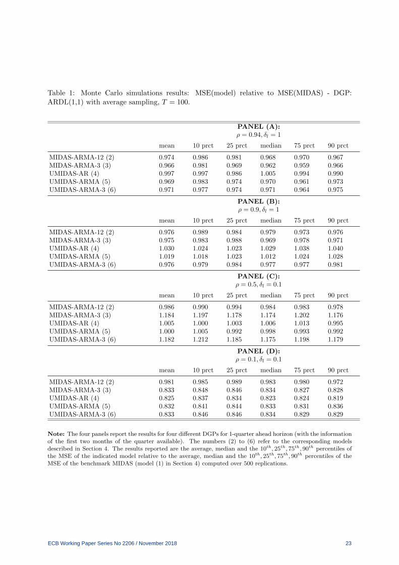
Table 1: Monte Carlo simulations results: MSE(model) relative to MSE(MIDAS) - DGP:ARDL(1,1) with average sampling, T = 100.

PANEL (A):ρ = 0.94, δl = 1

mean 10 prct 25 prct median 75 prct 90 prct

MIDAS-ARMA-12 (2) 0.974 0.986 0.981 0.968 0.970 0.967MIDAS-ARMA-3 (3) 0.966 0.981 0.969 0.962 0.959 0.966UMIDAS-AR (4) 0.997 0.997 0.986 1.005 0.994 0.990UMIDAS-ARMA (5) 0.969 0.983 0.974 0.970 0.961 0.973UMIDAS-ARMA-3 (6) 0.971 0.977 0.974 0.971 0.964 0.975

PANEL (B):ρ = 0.9, δl = 1



PANEL (C):ρ = 0.5, δl = 0.1



PANEL (D):ρ = 0.1, δl = 0.1



Note: The four panels report the results for four different DGPs for 1-quarter ahead horizon (with the informationof the first two months of the quarter available). The numbers (2) to (6) refer to the corresponding modelsdescribed in Section 4. The results reported are the average, median and the 10th, 25th, 75th, 90th percentiles ofthe MSE of the indicated model relative to the average, median and the 10th, 25th, 75th, 90th percentiles of theMSE of the benchmark MIDAS (model (1) in Section 4) computed over 500 replications.


Table 2: Monte Carlo simulations results: MSE(model) relative to MSE(MIDAS) - DGP:ARDL(1,1) with average sampling, T = 50

PANEL (A):ρ = 0.94, δl = 1



PANEL (B):ρ = 0.9, δl = 1


MIDAS-ARMA-12 (2) 0.997 1.001 1.012 0.994 0.986 0.982

MIDAS-ARMA-3 (3) 0.973 0.978 1.006 0.964 0.961 0.977UMIDAS-AR (4) 1.033 1.074 1.041 1.025 1.034 1.013UMIDAS-ARMA (5) 1.020 1.041 1.040 1.018 1.019 1.016UMIDAS-ARMA-3 (6) 0.981 0.982 1.023 0.968 0.971 0.983

PANEL (C):ρ = 0.5, δl = 0.1



PANEL (D):ρ = 0.1, δl = 0.1



Note: See Table 2.


Table 3: Monte Carlo simulations results: MSE(model) relative to MSE(MIDAS) - DGP:ARDL(2,2) with point-in-time sampling, T = 100

PANEL (A):ρ1 = 0.05, ρ2 = 0.1, δl1 = 0.5, δl2 = 1



PANEL (B):ρ1 = 0.125, ρ2 = 0.5, δl1 = 0.125, δl2 = 0.5



PANEL (C):ρ1 = 0.25, ρ2 = 0.5, δl1 = 0.5, δl2 = 1



Note: The four panels report the results for three different DGPs. The numbers (2) to (6) refer to the corre-sponding models described in Section 4. The results reported are the average, median and the 10th, 25th, 75th, 90th

percentiles of the MSE of the indicated model relative to the average, median and the 10th, 25th, 75th, 90th per-centiles of the MSE of the benchmark MIDAS (model (1) in Section 4) computed over 500 replications.


Table 4: Monte Carlo simulations results: MSE(model) relative to MSE(MIDAS) - DGP:ARDL(2,2) with point-in-time sampling, T = 50

PANEL (A):ρ1 = 0.05, ρ2 = 0.1, δl1 = 0.5, δl2 = 1



PANEL (B):ρ1 = 0.125, ρ2 = 0.5, δl1 = 0.125, δl2 = 0.5



PANEL (C):ρ1 = 0.25, ρ2 = 0.5, δl1 = 0.5, δl2 = 1



Note: see Table 3.


Tab

le5:

Dat

ad

escr

ipti

on

Series

Source

SourceCode

Tra

nsform

ation

Fre

quency

US

data

GD

PD

eflat

or

FR

ED

GD

PD

EF

Log

-diff

eren

ceQ

uar

terl

yR

eal

GD

PF

RE

DG

DP

Log

-diff

eren

ceQ

uar

terl

yP

riva

teN

onre

sid

enti

alF

ixed

Inve

stm

ent

FR

ED

PN

FI

Lev

elQ

uar

terl

yN

onre

sid

enti

al(i

mp

lici

tp

rice

defl

ator

)F

RE

DA

008R

D3Q

086S

BE

AL

evel

Qu

arte

rly

Rea

lP

riva

teN

onre

sid

enti

alF

ixed

Inve

stm

ent

PN

FI

/A

008R

D3Q

086S

BE

AL

og-d

iffer

ence

Qu

arte

rly

Con

sum

erP

rice

Ind

ex(C

PI)

FR

ED

CP

IAU

CS

LL

og-d

iffer

ence

Mon

thly

Per

son

alC

onsu

mp

tion

Exp

end

itu

res:

Pri

ceIn

dex

(PC

E)

FR

ED

PC

EP

IL

og-d

iffer

ence

Mon

thly

Em

plo

ym

ent

FR

ED

PA

YE

MS

Log

-diff

eren

ceM

onth

lyIn

du

stri

alP

rod

uct

ion

FR

ED

IND

PR

OL

og-d

iffer

ence

Mon

thly


Table 6: Forecasting U.S. GDP growth

Explanatory variable: Explanatory variable:Industrial production growth Employment growth

h=1 h=1MSE MAE MSE MAE

Value Ratio DM Value Ratio DM Value Ratio DM Value Ratio DMMIDAS-AR-12 4.06 1.00 NaN 1.58 1.00 NaN 4.84 1.00 NaN 1.73 1.00 NaNMIDAS-ARMA-12lags 4.05 1.00 0.41 1.59 1.01 0.13 4.73 0.98 0.33 1.72 0.99 0.37MIDAS-ARMA-3 4.27 1.05 0.07 1.60 1.01 0.22 4.76 0.98 0.39 1.72 0.99 0.42UMIDAS-biclags 4.21 1.04 0.15 1.58 1.00 0.41 4.70 0.97 0.31 1.73 1.00 0.49UMIDAS-ARMA-biclags 4.18 1.03 0.19 1.59 1.01 0.26 4.37 0.90 0.05 1.67 0.96 0.17UMIDAS-ARMA-3 4.27 1.05 0.07 1.60 1.01 0.22 4.76 0.98 0.39 1.72 0.99 0.42AR 7.60 1.87 0.01 1.97 1.25 0.01 7.60 1.57 0.02 1.97 1.14 0.05







Note: The table reports the results on the forecasting performance of the different models. In the columns”value” we report the MSE and the MAE respectively. In the columns ”ratio” we report the MSE and MAE ofeach model relative to the MIDAS-AR benchmark. In the columns ”DM” we report the p-value of the Diebold-Mariano test. The forecasts are evaluated over the sample 1980Q1-2015Q4. The lowest values for each variableare underlined.


Table 7: Forecasting U.S. Real Private Nonresidential Fixed Investment growth





Value Ratio DM Value Ratio DM Value Ratio DM Value Ratio DMMIDAS-AR-12 38.90 1.00 NaN 4.72 1.00 NaN 36.33 1.00 NaN 4.71 1.00 NaNMIDAS-ARMA-12 38.59 0.99 0.34 4.74 1.00 0.37 36.13 0.99 0.40 4.74 1.01 0.32MIDAS-ARMA-3 41.46 1.07 0.07 4.86 1.03 0.11 36.70 1.01 0.29 4.76 1.01 0.21UMIDAS-biclags 41.92 1.08 0.00 4.87 1.03 0.00 37.84 1.04 0.03 4.78 1.02 0.08UMIDAS-ARMA-biclags 44.76 1.15 0.00 5.11 1.08 0.00 38.40 1.06 0.03 4.85 1.03 0.07UMIDAS-ARMA-3 43.93 1.13 0.03 4.92 1.04 0.06 36.69 1.01 0.36 4.80 1.02 0.11AR 47.14 1.21 0.08 5.18 1.10 0.05 47.14 1.30 0.04 5.18 1.10 0.05





Note: See Table 6.


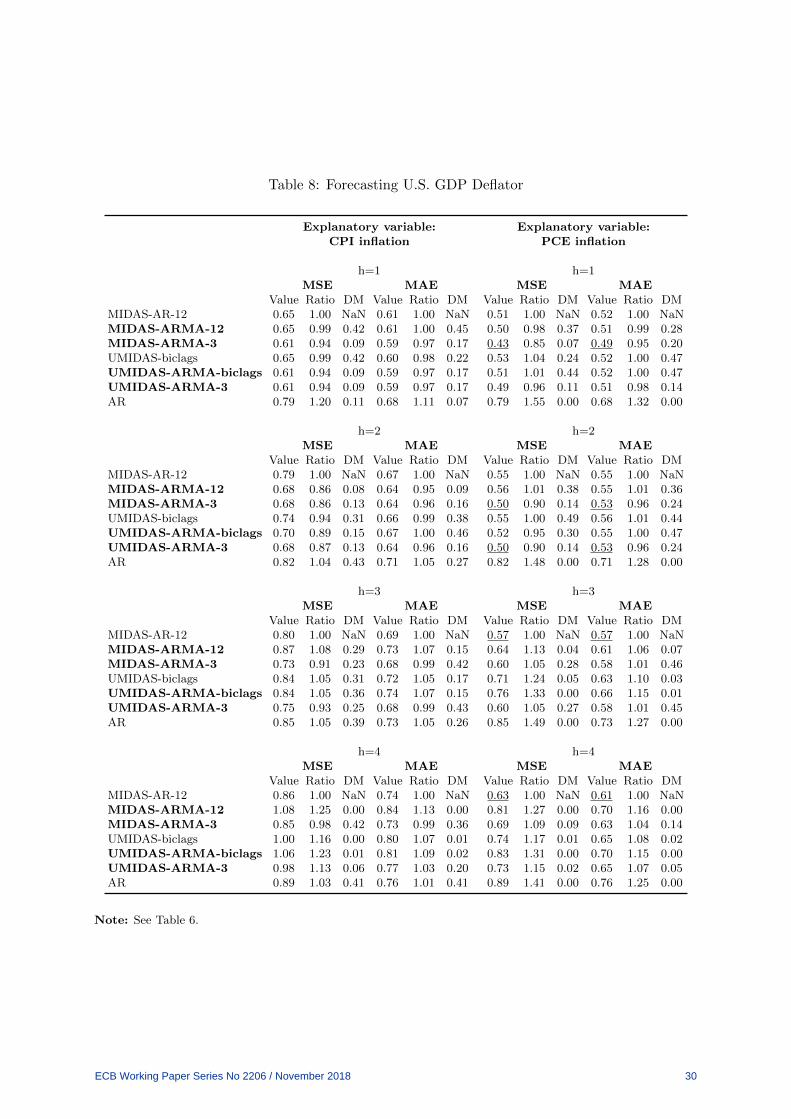
Table 8: Forecasting U.S. GDP Deflator

Explanatory variable: Explanatory variable:CPI inflation PCE inflation









Note: See Table 6.


Table 9: Bias/Variance decomposition of MSE

Bias Variance

h=1 h=2 h=3 h=4 h=1 h=2 h=3 h=4GDP with MIDAS1-AR-12lags 1.00 1.00 1.00 1.00 1.00 1.00 1.00 1.00Industrial MIDAS-ARMA-12lags 0.72 0.68 0.59 0.89 1.00 0.97 1.04 0.94Production MIDAS-ARMA-3lags 0.85 0.97 1.01 0.90 1.06 0.99 0.91 0.90

UMIDAS-biclags 1.09 1.04 1.08 0.87 1.04 1.06 0.99 0.97UMIDAS-ARMA-biclags 0.96 1.03 1.13 1.06 1.03 1.03 1.50 0.97UMIDAS-ARMA-3lags 0.85 1.12 1.23 0.98 1.06 1.05 1.00 1.10AR 3.06 1.02 1.23 1.01 1.84 1.17 1.07 0.95

GDP with MIDAS1-AR-12lags 1.00 1.00 1.00 1.00 1.00 1.00 1.00 1.00Employment MIDAS-ARMA-12lags 0.26 0.70 2.22 1.69 0.98 0.92 0.95 0.93

MIDAS-ARMA-3lags 0.18 1.44 0.51 0.65 0.98 0.94 0.82 0.94UMIDAS-biclags 5.60 1.00 0.51 0.74 0.97 1.00 0.89 0.95UMIDAS-ARMA-biclags 19.59 1.52 1.88 1.30 0.90 0.95 1.71 0.97UMIDAS-ARMA-3lags 0.18 1.40 0.56 0.61 0.98 1.00 0.93 0.88AR 348.15 4.11 0.87 0.56 1.51 1.24 1.00 0.81

PNFI with MIDAS1-AR-12lags 1.00 1.00 1.00 1.00 1.00 1.00 1.00 1.00Industrial MIDAS-ARMA-12lags 5.39 0.94 0.86 0.86 0.95 0.99 0.96 0.96Production MIDAS-ARMA-3lags 10.55 1.13 1.54 1.12 0.91 1.07 1.05 0.95


PNFI with MIDAS1-AR-12lags 1.00 1.00 1.00 1.00 1.00 1.00 1.00 1.00Employment MIDAS-ARMA-12lags 0.99 1.15 0.00 0.73 1.01 0.99 0.93 0.86

MIDAS-ARMA-3lags 0.78 0.42 4.78 0.17 1.01 1.01 0.94 0.72UMIDAS-biclags 0.91 0.85 0.35 0.24 1.01 1.04 1.04 0.86UMIDAS-ARMA-biclags 0.81 0.32 7.20 0.23 1.04 1.06 0.97 0.84UMIDAS-ARMA-3lags 0.78 0.44 4.22 0.23 1.01 1.01 0.94 0.80AR 0.25 2.53 230.03 0.58 1.40 1.29 1.25 0.93

GDP Deflator MIDAS1-AR-12lags 1.00 1.00 1.00 1.00 1.00 1.00 1.00 1.00with CPI MIDAS-ARMA-12lags 1.08 0.79 0.83 0.95 0.98 0.88 1.15 1.35inflation MIDAS-ARMA-3lags 0.87 0.61 0.51 0.72 0.94 0.92 1.03 1.07


GDP Deflator MIDAS1-AR-12lags 1.00 1.00 1.00 1.00 1.00 1.00 1.00 1.00with PCE MIDAS-ARMA-12lags 1.23 1.00 0.88 1.04 0.97 1.01 1.19 1.33inflation MIDAS-ARMA-3lags 0.45 0.58 0.62 0.77 0.87 0.95 1.15 1.17


Note: The table the decomposition of the MSE of the different models as presented in Section 4 into bias andvariance, for different forecasting horizons. The forecasts are evaluated over the sample 1980Q1-2015Q4. Thenumbers reported are the ratio of the bias and of the variance of each model relative to the bias and variance ofthe MIDAS-AR model.


Table 10: Full-sample estimated MA coefficients

Forecasting U.S. GDP growth

Explanatory variable: Explanatory variable:Industrial Production Employment

h=1 h=2 h=3 h=4 h=1 h=2 h=3 h=4MA(1) MA(1) MA(2) MA(1) MA(1) MA(1) MA(1) MA(1) MA(1)

MIDAS-ARMA-12lags 0.06 0.03 0.11 0.29 0.26 0.39 0.35 0.24 0.12(0.45) (0.46) (0.72) (1.33) (0.78) (3.59) (2.26) (1.18) (0.42)

MIDAS-ARMA-3lags -0.10 0.05 0.17 0.31 0.32 0.41 0.44 0.37 0.26(-0.89) (0.73) (1.13) (1.71) (1.20) (4.00) (2.85) (1.95) (1.01)

UMIDAS-ARMA-biclags 0.01 0.06 0.19 0.11 0.25 0.05 0.42 0.25 0.28(0.08) (0.84) (1.14) (0.43) (1.22) (0.18) (2.98) (1.47) (1.15)

UMIDAS-ARMA-3lags -0.10 0.05 0.17 0.31 0.16 0.41 0.45 0.33 0.27(-0.89) (0.73) (1.13) (1.80) (0.60) (4.00) (3.03) (1.70) (1.07)

Forecasting PNFI growth

Explanatory variable: Explanatory variable:Industrial Production Employment

h=1 h=2 h=3 h=4 h=1 h=2 h=3 h=4MA(1) MA(1) MA(1) MA(1) MA(1) MA(1) MA(1) MA(1)

MIDAS-ARMA-12lags -0.33 -0.14 0.13 -0.03 0.13 0.29 0.35 0.46(-3.82) (-1.15) (0.65) (-0.13) (1.27) (2.22) (2.37) (2.67)

MIDAS-ARMA-3lags -0.39 -0.14 0.15 -0.07 0.11 0.27 0.37 0.48(-5.83) (-1.54) (1.14) (-0.43) (1.23) (2.86) (2.65) (2.94)

UMIDAS-ARMA-biclags -0.31 0.05 0.17 -0.09 -0.04 0.26 0.35 0.48(-3.70) (0.50) (1.33) (-0.51) (-0.42) (2.78) (2.41) (2.46)

UMIDAS-ARMA-3lags -0.39 -0.12 0.15 -0.07 0.08 0.29 0.37 0.48(-5.83) (-1.24) (1.14) (-0.43) (0.83) (3.00) (2.65) (2.98)

Note: The table reports the estimated values of MA coefficients using the full sample 1960-2015. The val-ues in parentheses are t-statistics calculated with Newey-West standard errors to take into account the serialautocorrelation of order h− 1, possibly induced by direct forecasting.


Table 11: Full-sample estimated MA coefficients

Forecasting U.S. GDP deflator

Explanatory variable:Consumer Price Index

h=1 h=2 h=3 h=4MA(1) MA(2) MA(1) MA(2) MA(1) MA(2) MA(1) MA(2)

MIDAS-ARMA-12lags .-0.09 -0.31 0.18 -0.30 0.29 -0.08 0.19 0.14(-1.03) (-2.43) (1.89) (-2.78) (2.78) (-0.67) (1.70) (1.46)

MIDAS-ARMA-3lags -0.09 -0.36 0.20 -0.34 0.28 -0.10 0.18 0.11(-1.13) (-4.65) (2.09) (-4.48) (2.99) (-0.93) (1.76) (1.08)

UMIDAS-ARMA-biclags -0.09 -0.36 0.18 -0.35 0.25 -0.12 0.16 0.09(-1.13) (-4.65) (1.78) (-4.58) (2.62) (-1.09) (1.58) (0.91)

UMIDAS-ARMA-3lags -0.09 -0.36 0.20 -0.34 0.28 -0.10 0.18 0.11(-1.13) (-4.65) (2.06) (-4.44) (2.99) (-0.93) (1.76) (1.08)

Explanatory variable:PCE Price Index

h=1 h=2 h=3 h=4MA(1) MA(2) MA(1) MA(2) MA(1) MA(2) MA(1) MA(2)

MIDAS-ARMA-12lags -0.06 0.09 0.13 -0.22 0.25 -0.03 0.19 0.19(-0.68) (0.55) (1.50) (-1.62) (2.48) (-0.30) (1.84) (2.07)

MIDAS-ARMA-3lags 0.15 0.32 0.14 -0.30 0.24 -0.05 0.18 0.16(1.97) (3.25) (1.56) (-3.86) (2.95) (-0.53) (1.91) (1.53)

UMIDAS-ARMA-biclags -0.13 -0.29 0.14 -0.30 0.22 -0.06 0.17 0.16(-1.84) (-3.60) (1.56) (-3.86) (2.63) (-0.63) (1.82) (1.51)

UMIDAS-ARMA-3lags -0.13 -0.29 0.14 -0.30 0.24 -0.05 0.18 0.16(-1.84) (-3.60) (1.56) (-3.86) (2.95) (-0.53) (1.91) (1.53)

Note: The table reports the estimated values of MA coefficients using the full sample 1960-2015. The val-ues in parentheses are t-statistics calculated with Newey-West standard errors to take into account the serialautocorrelation of order h− 1, possibly induced by direct forecasting.


Fig

ure

1:O

ut-

of-s

amp

lep

erfo

rman

ce:

one-

qu

arte

rah

ead

(a)

GD

Pw

ith

mon

thly

ind

ust

rial

pro

du

ctio

n(b

)P

NF

Iw

ith

mon

thly

ind

ust

rial

pro

du

ctio

n

(c)

GD

Pd

eflat

orw

ith

mon

thly

CP

I(d

)G

DP

defl

ator

wit

hm

onth

lyP

CE


Fig

ure

2:O

ut-

of-s

amp

lep

erfo

rman

ce:

fou

r-qu

arte

rsah

ead

(a)

GD

Pw

ith

mon

thly

emp

loym

ent

(b)

PN

FI

wit

hm

onth

lyem

plo

ym

ent

(c)

GD

Pd

eflat

orw

ith

mon

thly

CP

I(d

)G

DP

defl

ator

wit

hm

onth

lyP

CE


Appendix for “Mixed frequency mod-els with MA components”

A Estimation of (U)MIDAS-ARMA models

In this section we detail the algorithm used to estimate the (U)MIDAS-ARMA models with

non-linear least squares (NLS).

A.1 NLS estimation of MIDAS-ARMA

The MIDAS-ARMA specification is as in (15):

ytm = c(Lm)ytm−hm + βB(L, θ)xtm−hm+w + utm + q(Lm)utm−hm .

The estimation procedure, for given orders of the lag polynomials, consists of the following steps:

Step 1 Get initial values for all the parameters but q(Lm) following Foroni et al. (2015) (the

starting values are chosen with a grid search over a set of values for θ, which minimize the

residual sum of squares). Set the initial values for q(Lm). We initialize the MA coefficients

by a draw from the uniform U(0.1, 0.5) distribution. In principle, it is possible to include

the selection of initial value of q(Lm) into the grid search.

Step 2 Estimate all the parameters, including the weights in the Almon polynomial, simultane-

ously by NLS, numerically minimizing the residual sum of squares, starting from the initial

values obtained in Step 1.

A.2 NLS estimation of UMIDAS-ARMA

The UMIDAS-ARMA specification is as in (13):

ytm = c(Lm)ytm−hm + δ(L)xtm−hm+w + utm + q(Lm)utm−hm ,

with p, d and r being the lag orders of c(Lm), δ(L) and q(Lm) respectively. The estimation

procedure consists of the following steps:


Step 1 Get the initial values for all the parameters but q(Lm) by projecting ytm on∑p

j=0 ytm−hm−j

and∑d

j=0 xtm−hm+w−j . Set the initial value for q(Lm). We initialize the MA coefficients

by a draw from the uniform U(0.1, 0.5) distribution. In principle, it is possible to perform

a grid search and find a set of starting values of q(Lm) which minimize the residual sum

of squares.

Step 2 Estimate all the parameters simultaneously by NLS, numerically minimizing the residual

sum of squares, starting from the initial values obtained in Step 1.

B Monte Carlo experiments: robustness checks

We run a battery of robustness checks on our Monte Carlo experiments.

1. We modify the set up by reducing the explanatory power of the x variable in such a way

that the total R2 of the DGP for y is equal to 0.3, 0.5 and 0.7. We obtain that by changing

the value of the variance of extm in the DGP for x. As examples, we consider the cases

with a less persistent AR component, ρ = 0.5, where it is more likely to have a smaller R2.

The rest of the simulation is set up according to the DGP1 described in Section 4.1. The

results are shown in Table B.1, and are similar to those in the main analysis. In general,

adding an MA component (especially to the MIDAS) still improves the performance of the

models.

2. We take again DGP1, and keep everything the same, except the sample size. We consider a

longer estimation sample, with Tq = 200, which corresponds to 50 years of quarterly obser-

vations. The results are shown in Table B.2. The long sample does not affect substantially

the findings.

3. We evaluate the results for DGP1 also at 2- and 4-quarter ahead horizons. The results are

shown in Tables B.3 and B.4. At 2-quarter ahead horizon, adding an MA component is

generally still useful, while at 4-quarter ahead horizon the MA is not useful anymore.


Table B.1: Robustness check: x explains a smaller share of y

DGP: average sampling, ρ = 0.5, δl = 0.1, T = 100, h = 1

PANEL (A):R2 = 0.3

mse 10 prct 25 prct median 75 prct 90 prctMIDAS-ARMA-12lags 1.020 1.034 0.989 1.017 1.013 1.072MIDAS-ARMA-3lags 1.009 1.027 1.000 1.032 1.010 0.998UMIDAS-biclags 1.023 1.030 1.031 1.047 1.019 0.986UMIDAS-ARMA-biclags 1.040 1.065 1.012 1.048 1.037 1.035UMIDAS-ARMA-3lags 1.027 1.048 1.012 1.044 1.024 1.008

PANEL (B):R2 = 0.5


PANEL (C):R2 = 0.7


Note: The table is organized as Table 1 in Section 4.


Table B.2: Robustness check: longer sample T = 200

DGP: average sampling, T = 200, h = 1

PANEL (A):ρ = 0.94, δl = 1


PANEL (B):ρ = 0.9, δl = 1


PANEL (C):ρ = 0.5, δl = 0.1


PANEL (D):ρ = 0.1, δl = 0.1


Note: The table is organized as Table 1 in Section 4.


Table B.3: Robustness check: forecasting 2 quarters ahead

DGP: average sampling, T=100, h=2

PANEL (A):ρ = 0.94, δl = 1


PANEL (B):ρ = 0.9, δl = 1


PANEL (C):ρ = 0.5, δl = 0.1


PANEL (D):ρ = 0.1, δl = 0.1


Note: The table is organized as Table 1 in Section 4. The forecasting horizon is 2 quarters ahead.


Table B.4: Robustness check: forecasting 4 quarters ahead

DGP: average sampling, T=100, h=4

PANEL (A):ρ = 0.94, δl = 1

mse 10 prct 25 prct median 75 prct 90 prctMIDAS-ARMA-12lags 1.130 1.005 1.050 1.154 1.217 1.110MIDAS-ARMA-3lags 1.076 0.951 1.154 1.127 1.078 1.039

UMIDAS-biclags 0.976 0.921 1.021 1.036 1.015 0.946UMIDAS-ARMA-biclags 1.057 0.937 1.172 1.069 1.069 1.042

UMIDAS-ARMA-3lags 1.078 0.962 1.255 1.115 1.056 1.038

PANEL (B):ρ = 0.9, δl = 1



UMIDAS-ARMA-3lags 1.077 1.099 1.202 1.063 0.966 1.011

PANEL (C):ρ = 0.5, δl = 0.1



UMIDAS-ARMA-3lags 1.091 1.126 1.076 1.122 1.058 1.024

PANEL (D):ρ = 0.1, δl = 0.1



UMIDAS-ARMA-3lags 1.030 1.138 1.016 1.000 1.021 1.059

Note: The table is organized as Table 1 in Section 4. The forecasting horizon is 4 quarters ahead.


C Empirical applications: robustness checks

To see whether our results are robust, we run several additional exercises.

1. We recompute the forecast evaluation stopping our evaluation sample in 2007Q3, to exclude

the possibility that they are driven by the Great Recession. Tables C.1 to C.3 are the

equivalent of Tables 6 to 8 for the full sample. Results do not change substantially, and

remain broadly supportive of the inclusion of the MA component in the mixed-frequency

models. In most of the cases, the best performing model up to 2007 stays the best in the

full sample also. Also the magnitude of improvements is very comparable.

2. While in Section 5 we report only the results when two months of monthly information are

available, here we complete the set of possible results, considering the cases when only one

month of the quarter is available or when all three months are available. Results are re-

ported in Table C.4. Inclusion of the MA component helps at all horizons and, as expected,

the absolute performance generally improves when adding additional information.

3. We reestimate our models with real-time data. In particular:

• For forecasting GDP deflator inflation: GDP deflator is from Philadelphia Fed (GDPDEF).

CPI and PCEPI are from Alfred. CPI vintages are available only from 1994M02, so

the out-of-sample period in the exercise with GDPDEF / CPI starts on 1994Q2.

PCEPI vintages are available only from 2007M07, so the out-of-sample period in the

exercise for GDPDEF / PCEPI starts on 2000Q3.

• For forecasting GDP growth: GDP, industrial production and employment are all

available from Philadelphia Fed real-time data base. All vintages are available so the

out-of-sample period is the same as with historical data: 1980Q1-2015Q4.

• For forecasting Investment growth: we use Real Gross Private Domestic Investment:

nonresidential (RINVBF) available from Philadelphia Fed (we were not able to con-

struct Real PNFI in real-time.). Industrial production and employment are the same

as in GDP exercise. The out-of-sample period is 1980Q1 - 2015Q4.

In evaluating the forecasts we consider as realized values those in the vintage of 2016Q1.

Results are available in Tables C.5 to C.7. The main findings Inclusion of the MA compo-


nent helps at all horizons and, as expected, the absolute performance generally improves

when adding additional information.


Table C.1: Forecasting U.S. GDP growth: evaluation sample 1980Q1- 2007Q3










Note: The table reports the results on the forecasting performance of the different models. In the columns”value” we report the MSE and the MAE respectively. In the columns ”ratio” we report the MSE and MAE ofeach model relative to the MIDAS-AR benchmark. In the columns ”DM” we report the p-value of the Diebold-Mariano test. The forecasts are evaluated over the sample 1980Q1-2007Q3. The lowest values for each variableare underlined.


Table C.2: Forecasting U.S. Real Private Nonresidential Fixed Investment growth growth: eval-uation sample 1980Q1- 2007Q3










Note: See Table C.1.


Table C.3: Forecasting U.S. GDP Deflator: evaluation sample 1980Q1- 2007Q3

Explanatory variable: Explanatory variable:CPI inflation PCE inflation









Note: See Table C.1.


Table C.4: Nowcasting when one month of information is available (hm = 2) or all months ofinformation are available (hm = 0)

Forecasting GDP deflator with CPI inflation

hm = 2 hm = 0MSE MAE MSE MAE

Value Ratio DM Value Ratio DM Value Ratio DM Value Ratio DMMIDAS-AR-12 0.76 1.00 NaN 0.67 1.00 NaN 0.71 1.00 NaN 0.63 1.00 NaNMIDAS-ARMA-12 0.72 0.95 0.08 0.65 0.98 0.12 0.66 0.92 0.24 0.62 0.99 0.41MIDAR-ARMA-3 0.77 1.01 0.46 0.65 0.98 0.39 0.69 0.97 0.40 0.64 1.02 0.36UMIDAS-biclags 0.70 0.92 0.19 0.66 0.98 0.37 0.66 0.92 0.13 0.60 0.96 0.12UMIDAS-ARMA-biclags 0.67 0.87 0.03 0.64 0.96 0.15 0.62 0.87 0.02 0.60 0.95 0.08UMIDAS-ARMA-3 0.73 0.95 0.12 0.66 0.99 0.40 0.65 0.91 0.11 0.61 0.96 0.17AR 0.79 1.03 0.41 0.68 1.03 0.35 0.79 1.10 0.26 0.68 1.08 0.14

Forecasting GDP deflator with PCE inflation

MIDAS-AR-12 0.68 1.00 NaN 0.63 1.00 NaN 0.54 1.00 NaN 0.52 1.00 NaNMIDAS-ARMA-12 0.65 0.95 0.20 0.61 0.96 0.08 0.61 1.14 0.16 0.61 1.18 0.00MIDAR-ARMA-3 0.67 0.98 0.42 0.61 0.97 0.29 0.66 1.23 0.04 0.62 1.20 0.00UMIDAS-biclags 0.66 0.97 0.39 0.63 1.00 0.49 0.53 0.99 0.43 0.52 1.00 0.48UMIDAS-ARMA-biclags 0.66 0.96 0.35 0.63 1.00 0.47 0.51 0.95 0.26 0.51 0.99 0.36UMIDAS-ARMA-3 0.65 0.96 0.25 0.62 0.99 0.31 0.51 0.94 0.21 0.51 0.99 0.45AR 0.79 1.15 0.12 0.68 1.08 0.11 0.79 1.47 0.02 0.68 1.32 0.00

Forecasting GDP with industrial production


Forecasting GDP with employment


Forecasting Real PNFI with industrial production


Forecasting Real PNFI with employment


Note: The table reports the results on the forecasting performance of the different models one quarter ahead,when one month of information is available or all months are available. In the columns ”value” we report theMSE and the MAE respectively. In the columns ”ratio” we report the MSE and MAE of each model relativeto the MIDAS-AR benchmark. In the columns ”DM” we report the p-value of the Diebold-Mariano test. Theforecasts are evaluated over the sample 1980Q1-2015Q4.


Tab

leC

.5:

For

ecas

tin

gU

.S.

GD

Pgr

owth

:re

al-t

ime

fore

cast

s

Fore

cast

ing

GD

Pw

ith

indust

rial

pro

duct

ion

hm

onth

=0

hm

onth

=1

hm

onth

=2

MS

EM

AE

MS

EM

AE

MS

EM

AE

Valu

eR

ati

oD

MV

alu

eR

ati

oD

MV

alu

eR

ati

oD

MV

alu

eR

ati

oD

MV

alu

eR

ati

oD

MV

alu

eR

ati

oD

MM

IDA

S-A

R-1

25.1

61.0

0N

aN

1.7

61.0

0N

aN

5.9

91.0

0N

aN

1.9

11.0

0N

aN

6.7

71.0

0N

aN

1.9

51.0

0N

aN

MID

AS-A

RM

A-1

25.2

31.0

10.0

71.7

91.0

10.0

26.1

51.0

30.0

91.9

31.0

10.2

16.7

61.0

00.4

91.9

51.0

00.4

6M

IDA

R-A

RM

A-3

5.2

51.0

20.1

21.8

01.0

20.0

16.1

01.0

20.1

51.9

11.0

00.4

66.8

31.0

10.2

51.9

61.0

00.3

9U

MID

AS-b

icla

gs

5.5

01.0

70.0

11.8

21.0

30.0

06.1

41.0

30.0

91.9

21.0

00.3

56.7

61.0

00.4

41.9

40.9

90.1

2U

MID

AS-A

RM

A-b

icla

gs

5.5

11.0

70.0

11.8

21.0

30.0

06.2

31.0

40.0

61.9

11.0

00.4

86.8

01.0

10.2

31.9

40.9

90.1

4U

MID

AS-A

RM

A-3

5.3

21.0

30.0

21.8

01.0

20.0

16.1

61.0

30.0

61.9

21.0

10.2

77.3

21.0

80.0

42.0

11.0

30.0

9A

R7.5

51.4

60.0

41.9

81.1

20.0

87.5

51.2

60.1

11.9

81.0

30.3

37.5

51.1

20.0

61.9

81.0

10.3

4

Fore

cast

ing

GD

Pw

ith

emplo

ym

ent

MID

AS-A

R-1

25.2

91.0

0N

aN

1.8

01.0

0N

aN

6.7

31.0

0N

aN

1.9

31.0

0N

aN

7.6

81.0

0N

aN

1.9

81.0

0N

aN

MID

AS-A

RM

A-1

24.9

80.9

40.0

71.7

50.9

70.0

76.6

00.9

80.0

71.9

10.9

90.1

07.3

80.9

60.1

31.9

70.9

90.1

9M

IDA

R-A

RM

A-3

4.9

60.9

40.0

61.7

50.9

70.0

96.5

90.9

80.0

31.9

10.9

90.0

57.2

40.9

40.0

91.9

50.9

80.0

9U

MID

AS-b

icla

gs

4.9

70.9

40.1

61.7

50.9

70.1

86.4

00.9

50.2

11.9

20.9

90.4

07.3

90.9

60.2

91.9

81.0

00.4

6U

MID

AS-A

RM

A-b

icla

gs

5.0

80.9

60.2

31.7

70.9

80.2

66.3

80.9

50.1

91.9

31.0

00.4

47.2

60.9

50.1

31.9

70.9

90.2

3U

MID

AS-A

RM

A-3

4.9

20.9

30.0

71.7

50.9

70.1

16.6

60.9

90.4

41.9

81.0

20.2

17.8

01.0

20.4

22.0

41.0

30.1

4A

R7.5

51.4

30.0

21.9

81.1

00.1

07.5

51.1

20.1

21.9

81.0

20.3

07.5

50.9

80.4

01.9

81.0

00.4

8

Note

:T

he

table

rep

ort

sth

ere

sult

son

the

fore

cast

ing

per

form

ance

of

the

diff

eren

tm

odel

s.In

the

colu

mns

”va

lue”

we

rep

ort

the

MSE

and

the

MA

Ere

spec

tivel

y.In

the

colu

mns

”ra

tio”

we

rep

ort

the

MSE

and

MA

Eof

each

model

rela

tive

toth

eM

IDA

S-A

Rb

ench

mark

.In

the

colu

mns

”D

M”

we

rep

ort

the

p-v

alu

eof

the

Die

bold

-Mari

ano

test

.T

he

fore

cast

sare

evalu

ate

don

the

sam

ple

1980Q

1-2

015Q

4.


Tab

leC

.6:

For

ecas

tin

gU

.S.

Rea

lG

ross

Pri

vate

Dom

esti

cIn

vest

men

t-

Non

resi

den

tial:

real-

tim

efo

reca

sts

hm

onth

=0

hm

onth

=1

hm

onth

=2

MS

EM

AE

MS

EM

AE

MS

EM

AE

Valu

eR

ati

oD

MV

alu

eR

ati

oD

MV

alu

eR

ati

oD

MV

alu

eR

ati

oD

MV

alu

eR

ati

oD

MV

alu

eR

ati

oD

MM

IDA

S-A

R-1

233.2

21.0

0N

aN

4.5

91.0

0N

aN

37.2

91.0

0N

aN

4.9

51.0

0N

aN

43.0

41.0

0N

aN

5.2

71.0

0N

aN

MID

AS-A

RM

A-1

233.1

71.0

00.4

94.4

50.9

70.1

232.9

50.8

80.0

04.5

40.9

20.0

042.0

60.9

80.2

55.0

90.9

70.0

3M

IDA

R-A

RM

A-3

33.1

21.0

00.4

84.4

90.9

80.2

434.7

00.9

30.0

74.7

10.9

50.0

441.4

70.9

60.0

65.1

10.9

70.0

3U

MID

AS-b

icla

gs

41.1

61.2

40.0

15.0

61.1

00.0

141.2

41.1

10.0

65.1

31.0

30.0

946.1

51.0

70.1

25.4

51.0

30.0

7U

MID

AS-A

RM

A-b

icla

gs

33.8

51.0

20.3

64.5

60.9

90.3

932.7

20.8

80.0

14.5

80.9

20.0

040.6

30.9

40.0

85.1

70.9

80.1

5U

MID

AS-A

RM

A-3

33.1

91.0

00.4

94.4

60.9

70.1

533.2

30.8

90.0

14.5

10.9

10.0

041.4

60.9

60.1

05.1

00.9

70.0

5A

R54.0

61.6

30.0

15.7

71.2

60.0

054.0

61.4

50.0

15.7

71.1

60.0

054.0

61.2

60.0

45.7

71.0

90.0

3

Fore

cast

ing

Rea

lG

ross

Pri

vate

Dom

esti

cIn

ves

tmen

t:N

onre

siden

tial

(RIN

VB

F)

wit

hem

plo

ym

ent

MID

AS-A

R-1

242.0

21.0

0N

aN

5.1

61.0

0N

aN

43.6

81.0

0N

aN

5.1

51.0

0N

aN

44.1

31.0

0N

aN

5.1

61.0

0N

aN

MID

AS-A

RM

A-1

241.9

81.0

00.4

65.1

61.0

00.4

743.4

61.0

00.3

95.1

61.0

00.3

945.0

21.0

20.0

65.1

71.0

00.4

6M

IDA

R-A

RM

A-3

42.5

81.0

10.3

55.1

30.9

90.3

143.1

10.9

90.2

05.1

51.0

00.4

944.4

51.0

10.3

05.1

51.0

00.4

2U

MID

AS-b

icla

gs

43.0

21.0

20.2

25.1

91.0

10.3

344.4

61.0

20.2

85.1

91.0

10.2

843.7

80.9

90.2

25.1

40.9

90.1

9U

MID

AS-A

RM

A-b

icla

gs

41.5

10.9

90.3

25.1

30.9

90.2

944.0

21.0

10.4

15.1

81.0

10.3

443.9

10.9

90.4

05.1

30.9

90.2

8U

MID

AS-A

RM

A-3

41.3

10.9

80.2

75.0

80.9

80.0

842.9

40.9

80.1

65.1

51.0

00.4

944.5

11.0

10.2

75.1

41.0

00.3

3A

R54.0

61.2

90.0

85.7

71.1

20.0

554.0

61.2

40.1

05.7

71.1

20.0

454.0

61.2

30.0

65.7

71.1

20.0

2

Note

:T

he

table

rep

ort

sth

ere

sult

son

the

fore

cast

ing

per

form

ance

of

the

diff

eren

tm

odel

s.In

the

colu

mns

”va

lue”

we

rep

ort

the

MSE

and

the

MA

Ere

spec

tivel

y.In

the

colu

mns

”ra

tio”

we

rep

ort

the

MSE

and

MA

Eof

each

model

rela

tive

toth

eM

IDA

S-A

Rb

ench

mark

.In

the

colu

mns

”D

M”

we

rep

ort

the

p-v

alu

eof

the

Die

bold

-Mari

ano

test

.T

he

fore

cast

sare

evalu

ate

don

the

sam

ple

1980Q

1-2

015Q

4.


Tab

leC

.7:

For

ecas

tin

gU

.S.

GD

Pd

eflat

or:

real

-tim

efo

reca

sts

Fore

cast

ing

GD

Pdefl

ato

rw

ith

CP

Iin

flati

on

hm

onth

=0

hm

onth

=1

hm

onth

=2

MS

EM

AE

MS

EM

AE

MS

EM

AE

Valu

eR

ati

oD

MV

alu

eR

ati

oD

MV

alu

eR

ati

oD

MV

alu

eR

ati

oD

MV

alu

eR

ati

oD

MV

alu

eR

ati

oD

MM

IDA

S-A

R-1

20.7

11.0

0N

aN

0.6

31.0

0N

aN

0.7

21.0

0N

aN

0.6

61.0

0N

aN

0.8

31.0

0N

aN

0.7

31.0

0N

aN

MID

AS-A

RM

A-1

20.6

20.8

80.1

80.6

10.9

70.3

30.6

70.9

30.0

90.6

30.9

50.0

80.7

50.9

00.0

40.7

00.9

60.0

8M

IDA

R-A

RM

A-3

0.6

90.9

70.4

10.6

20.9

90.4

60.6

40.8

80.0

20.6

20.9

30.0

40.9

51.1

30.2

10.7

51.0

40.3

2U

MID

AS-b

icla

gs

0.7

21.0

20.4

20.6

20.9

80.3

20.7

61.0

50.3

00.6

40.9

70.1

70.7

90.9

50.3

00.7

10.9

70.3

3U

MID

AS-A

RM

A-b

icla

gs

0.6

40.9

00.1

00.6

10.9

70.2

20.6

50.9

00.0

40.6

20.9

40.0

60.7

10.8

50.0

30.6

80.9

40.0

8U

MID

AS-A

RM

A-3

0.6

50.9

20.1

80.6

10.9

70.2

90.6

40.8

80.0

20.6

20.9

30.0

40.7

40.8

80.0

20.6

90.9

40.0

2A

R0.9

71.3

60.0

20.7

51.1

90.0

20.9

71.3

40.0

50.7

51.1

30.0

60.9

71.1

60.1

60.7

51.0

30.3

3

Fore

cast

ing

GD

Pdefl

ato

rw

ith

PC

Ein

flati

on

MID

AS-A

R-1

20.7

41.0

0N

aN

0.6

31.0

0N

aN

0.7

51.0

0N

aN

0.6

51.0

0N

aN

0.9

81.0

0N

aN

0.7

51.0

0N

aN

MID

AS-A

RM

A-1

20.7

71.0

40.4

10.6

91.0

90.1

50.7

00.9

30.1

40.6

10.9

40.0

50.8

70.8

90.0

80.7

30.9

70.3

0M

IDA

R-A

RM

A-3

0.8

71.1

70.1

30.7

01.1

10.0

80.7

10.9

50.2

30.6

51.0

00.4

90.9

91.0

10.4

80.7

51.0

00.5

0U

MID

AS-b

icla

gs

0.8

01.0

90.2

00.6

20.9

80.3

10.8

51.1

30.1

40.6

40.9

90.4

00.8

60.8

80.2

10.7

40.9

80.4

0U

MID

AS-A

RM

A-b

icla

gs

0.6

60.9

00.1

00.6

00.9

50.1

60.6

90.9

30.0

20.6

10.9

40.0

00.8

00.8

10.1

00.7

10.9

50.2

5U

MID

AS-A

RM

A-3

0.7

30.9

80.4

20.6

20.9

90.4

20.6

90.9

30.0

20.6

10.9

40.0

00.8

20.8

40.0

80.7

10.9

50.1

8A

R1.1

41.5

50.0

00.8

01.2

60.0

01.1

41.5

30.0

10.8

01.2

30.0

31.1

41.1

70.1

20.8

01.0

60.2

6

Note

:T

he

table

rep

ort

sth

ere

sult

son

the

fore

cast

ing

per

form

ance

of

the

diff

eren

tm

odel

s.In

the

colu

mns

”va

lue”

we

rep

ort

the

MSE

and

the

MA

Ere

spec

tivel

y.In

the

colu

mns

”ra

tio”

we

rep

ort

the

MSE

and

MA

Eof

each

model

rela

tive

toth

eM

IDA

S-A

Rb

ench

mark

.In

the

colu

mns

”D

M”

we

rep

ort

the

p-v

alu

eof

the

Die

bold

-Mari

ano

test

.T

he

fore

cast

sw

ith

CP

Iare

evalu

ate

don

the

sam

ple

1994Q

2-2

015Q

4,

while

those

wit

hP

CE

PI

are

evalu

ate

don

the

sam

ple

200Q

3-2

015Q

4


Acknowledgements The views expressed in this paper are those of the authors and do not necessarily coincide with the views of the European Central Bank or the Eurosystem. Aniss Benmoussa has provided excellent research assistance. We thank the editor Eric Ghysels and three anonymous referees for constructive comments. We thank Ana Galvão, Pierre Guérin, Helmut Luetkepohl, Christian Schumacher, the seminar participants at DIW, Maastricht University, and the participants to the ECB Workshop in Advances in short-term forecasting, the IWH-CIREQGW Macroeconometric Workshop, the CFE conference, the Barcelona Summer Forum, the CEF conference for the very useful comments. The third author acknowledges financial support from the Fonds de recherche sur la société et la culture (Québec) and the Social Sciences and Humanities Research Council.

Claudia Foroni European Central Bank, Frankfurt am Main, Germany; email: [email protected]

Massimiliano Marcellino Bocconi University, Milan, Italy; email: [email protected]

Dalibor Stevanović Université du Québec à Montréal, Montreal, Canada; email: [email protected]

© European Central Bank, 2018

Postal address 60640 Frankfurt am Main, Germany Telephone +49 69 1344 0 Website www.ecb.europa.eu

All rights reserved. Any reproduction, publication and reprint in the form of a different publication, whether printed or produced electronically, in whole or in part, is permitted only with the explicit written authorisation of the ECB or the authors.

This paper can be downloaded without charge from www.ecb.europa.eu, from the Social Science Research Network electronic library or from RePEc: Research Papers in Economics. Information on all of the papers published in the ECB Working Paper Series can be found on the ECB’s website.

PDF ISBN 978-92-899-3311-7 ISSN 1725-2806 doi:10.2866/395141 QB-AR-18-086-EN-N

mailto:[email protected]



http://www.ecb.europa.eu/

http://www.ecb.europa.eu/

http://ssrn.com/

https://ideas.repec.org/s/ecb/ecbwps.html

http://www.ecb.europa.eu/pub/research/working-papers/html/index.en.html

Working Paper Series - ecb.europa.eu · ator. The inclusion of an MA component generally improves...

Documents

Transcript of Working Paper Series - ecb.europa.eu · ator. The inclusion of an MA component generally improves...