WORKING PAPER ITLS-WP-11-19 A comparison of...
29
INSTITUTE of TRANSPORT and LOGISTICS STUDIES The Australian Key Centre in Transport and Logistics Management The University of Sydney Established under the Australian Research Council’s Key Centre Program. WORKING PAPER ITLS-WP-11-19 A comparison of algorithms for generating efficient choice experiments. By Wu Quan, John M. Rose, Andrew T. Collins and Michiel C.J. Bliemer 1 1 Delft University of Technology October 2011 ISSN 1832-570X
Transcript of WORKING PAPER ITLS-WP-11-19 A comparison of...

INSTITUTE of TRANSPORT and LOGISTICS STUDIES The Australian Key Centre in Transport and Logistics Management
The University of Sydney Established under the Australian Research Council’s Key Centre Program.
WORKING PAPER
ITLS-WP-11-19
A comparison of algorithms for generating efficient choice experiments. By Wu Quan, John M. Rose, Andrew T. Collins and Michiel C.J. Bliemer
1
1 Delft University of Technology October 2011 ISSN 1832-570X

NUMBER: Working Paper ITLS-WP-11-19
TITLE: A comparison of algorithms for generating efficient choice experiments.
ABSTRACT: Stated choice (SC) studies typically rely on the use of an underlying experimental design to construct the hypothetical choice situations shown to respondents. These designs are constructed by the analyst, with several different ways of constructing these designs having been proposed in the past. Recently, there has been a move from so-called orthogonal designs to more efficient designs. Efficient designs optimize the design such that the data will lead to more reliable parameter estimates for the model under consideration. The literature dealing with the generation of efficient designs has examined and largely solved the issue of a requirement for a prior knowledge of the parameter estimates that will be obtained post data collection. However, unlike orthogonal designs, the efficient design methodology requires the evaluation of a number of designs, and hence is computationally expensive to undertake. As such, the literature has suggested and implemented a number of algorithms to locate efficient designs for SC experiments. In this paper, we compare and contrast the performance of these algorithms as well as introduce two new algorithms.
KEY WORDS: Stated choice; efficient experimental designs; algorithms.
AUTHORS: Wu Quan, John Rose, Andrew Collins and Michiel Bliemer
CONTACT: INSTITUTE of TRANSPORT and LOGISTICS STUDIES (C37) The Australian Key Centre in Transport and Logistics Management The University of Sydney NSW 2006 Australia Telephone: +612 9351 0071 Facsimile: +612 9351 0088 E-mail: [email protected] Internet: http://sydney.edu.au/business/itls
DATE: October 2011

A comparison of algorithms for generating efficient choice experiments Quan, Rose, Collins & Bliemer
1
1. Introduction
Unlike most survey data where information on both the dependent and independent variables is captured directly from respondents, stated preference surveys, of which stated choice (SC) data is a special case, is unique in that typically only the dependent variable is provided by the respondent. In the main, the primary variables of interest consist of the attributes and their associated levels of competing alternatives grouped together in what are commonly referred to as choice tasks. Rather than present respondents with a single choice task, a typical transport SC study might involve respondents being asked to answer multiple choice tasks. Respondents are then asked to review each choice task and select their most preferred alternative from within each. Consequently, an archetypal SC experiment might require choice data collected from 200 respondents, each of whom were observed to answer between four to sixteen choice tasks, thus resulting in anywhere between 800 and 3200 choice observations.
Increasing evidence of both an empirical (e.g., Bliemer and Rose 2011; Louviere et al. 2008) and theoretical nature (e.g., Burgess and Street 2005; Sándor and Wedel 2001, 2002, 2005) suggests that the specific allocation of the attribute levels to the alternatives presented to respondents may impact to a greater or lesser extent upon the standard errors and covariances of the parameter outputs of discrete choice models, particularly when small samples are involved. As such, rather than simply randomly assign the attribute levels shown to respondents over the course of the survey, experimental design theory has traditionally been applied to allocate the attribute levels to the alternatives in some systematic manner.
The primary focus of research into experimental design theory as related to SC studies has tended to focus on producing designs which are deemed to be more statistically efficient. Within the literature, statistical efficiency has been related to the expected standard errors that a design will produce should it be used in practice. Designs that are expected to produce smaller standard errors, all else being equal, are said to be more statistically efficient (see e.g., Bliemer and Rose 2009; Huber and Zwerina 1996; Rose and Bliemer 2009; Sándor and Wedel 2001, 2002). As such, a direct link exists between the statistical efficiency of a design and the sample size requirements of SC studies, as a more efficient design would be expected to produce the same t-ratios as a less efficient design, but with a a smaller sample, or alternatively, produce larger t-ratios than a less efficient design given the same sample.
The fact that SC data is typically analysed using non-linear models such as the multinomial logit (MNL) and mixed multinomial logit (MMNL) models implies that the efficiency of a design will depend upon the unknown parameter vector (see Atkinson and Haines 1996). Given that the true parameter vector is unknown at the stage at which the design is to be generated, analysts are required to make assumptions about the specific values that the parameters might take. By assuming specific parameter values associated with a given design matrix X, it becomes possible to calculate the expected utilities for each of the alternatives. Once known, these expected utilities can in turn be used to calculate the likely choice probabilities. Next, given knowledge of the attribute levels (the design), expected parameter values and the resultant choice probabilities, it becomes a straightforward exercise to calculate the Fisher information matrix,
,NI which is computed as the negative expected second derivatives of the log-likelihood function of the model to be estimated, considering N respondents (see Train, 2009). The asymptotic variance-covariance (AVC) matrix, Ω ,N which is the inverse of the Fisher information matrix, can then be determined, and the expected standard errors thus derived. By manipulating the attribute levels of the alternatives, for known (assumed) parameter values, the analyst is able to minimize the elements within the AVC matrix, which in the case of the diagonals means lower standard errors and hence greater reliability in the estimates at a fixed sample size (or even at a reduced sample size).
Three different approaches to the problem of having to assume prior parameter estimates have been developed within the literature. The first is to assume a priori precise knowledge of the

A comparison of algorithms for generating efficient choice experiments Quan, Rose, Collins & Bliemer
2
parameter estimates, leading to what are termed locally optimal designs. These designs are called locally optimal designs, because they are optimised for these specific prior parameter values and quickly loose efficiency if the true parameter values differ to those that are assumed during the design generation phase. The most common assumption made is that of zero prior parameter values. In such cases, linear experimental design theories can be applied to solve the problem leading to the generation of designs which will be orthogonal in the attributes (see e.g., Anderson and Wiley 1992; Grossman et al. 2002; Kuhfeld et al. 1994; Lazari and Anderson 1994; Street et al. 2001, 2005). Alternatively, some researchers have generated locally optimal designs under non-zero prior parameter values (e.g., Carlsson and Martinsson 2002; Huber and Zwerina 1996). Under the assumption of non-zero prior parameter values, these researchers have found that non-orthogonal designs tend to be more statistically efficient than orthogonal designs.
The second and more recent approach has tended to integrate uncertainty surrounding the assumed parameter values via the use of Bayesian design methods (see e.g., Chaloner and Verdinelli 1995). First applied to SC experiments by Sandor and Wedel (2001), the use of these Bayesian methods involves assuming prior parameter distributions as opposed to specific fixed values and examining the AVC matrix generated over draws taken from these distributions. Such a design approach has shown to produce Bayesian optimal designs which are less efficient than correctly specified locally optimal designs but which are more robust to prior parameter misspecification (see e.g., Sandor and Wedel 2001). As with locally optimal designs assuming non-zero prior parameter values, non-orthogonal designs tend to be more statistically efficient under the assumption of Bayesian prior parameter distributions (see e.g., Kessels et al. 2009). Ongoing research efforts for this class of designs have tended to examine how best to represent the Bayesian prior parameter distributions (see e.g., Bliemer et al. 2008; Goegebeur et al. 2007; Yu et al. 2008, 2010).
A third approach assumes that priors are continuously updated by estimating the parameters on sub-samples while collecting the data. For each respondent (or batch of respondents), a new design is generated based on the currently set local or Bayesian priors. Such a process has been proposed by Kanninen (2002), and Bliemer and Rose (2009) have shown that such sequentially optimal designs can improve the efficiency of the design significantly, but comes at the cost of more complex data collection methods.
Independent of the prior parameters assumed, it is necessary to apply some form of objective function on which to judge the overall statistical efficiency of the design. A number of summary measures have been proposed within the literature, however the most predominately used measure appears to be the D-error statistic. The D-error statistic is calculated simply by taking the determinant of the AVC matrix assuming a single respondent, 1,Ω and normalising this value by the number of parameters, K. Minimizing the D-error statistic corresponds to minimizing, on average, the elements contained within the expected AVC matrix. Designs which minimize the D-error statistic are therefore called D- optimal designs, or D-efficient designs (as in most cases, we cannot prove the design is truly optimal).
Different D-error measures corresponding to the various assumptions about the prior parameter values have been proposed within the literature. For example Dz-efficient designs correspond to locally optimal designs assuming zero prior parameter values (see Equation 1) whereas locally optimal designs assuming non-zero priors have been termed Dp
θ
-efficient designs (see Equation 2). Designs generated assuming Bayesian parameter distributions (with distributional parameter priors ) are known as Bayesian or Db
-efficient designs (see Equation 3).

A comparison of algorithms for generating efficient choice experiments Quan, Rose, Collins & Bliemer
3
( )( )1
1det ,0 ,KzD error X− = Ω (1)
( )( )1
1det , ,KpD error X β− = Ω (2)
( )( ) ( )1
1det , | ,KbD error X d
ββ φ β θ β− = Ω∫ (3)
where ( )φ ⋅ is the (multivariate) probability density function of the assumed Bayesian distribution. Under assumptions of locally optimal non-zero prior parameters and Bayesian prior parameter distributions, non-orthogonal designs have been found to be more efficient than orthogonal designs. Unfortunately, unlike orthogonal designs for which there exist a finite number in practice, and where catalogs of available design matrices are available (see e.g., Hedayat et al. 1999), the fact that the efficiency of a design specifically depends upon the prior parameters assumed, which will generally differ from one study to next, means that any design approach that lets go of orthogonality will require that designs be generated on a case by case basis. It is for this reason that researchers have tended to rely on algorithms to search the possible design space for each unique SC problem (see e.g., Kessels et al. 2009).
The purpose of this paper is two-fold. Firstly, we seek to introduce and implement a number of new algorithms, or modifications of existing algorithms for generating SC experiments, the performance of which we compare to a number of existing algorithms. Secondly, a number of existing papers have examined the performance of various algorithms in the past, however these have assumed a MNL or cross sectional MMNL model specification. In this paper, we test the performance of the various algorithms on the panel specification of the MMNL model, a model which poses a number of unique challenges that do not exist for the class of models that have been examined within the literature to date. The remainder of this paper is broken down as follows. In the following section, we discuss general considerations when constructing SC experiments before the MNL and panel MMNL model specifications and their corresponding AVC matrices are discussed in Section 3. Next, various algorithms that may be used to locate efficient SC experimental designs are discussed in Section 4. In Section 5, we provide the results of two case studies after which we provide concluding comments.
2. Stated choice designs
When designing a stated choice study, a number of decisions must be made about the properties of the choice task, including whether it is labeled or unlabeled, the number of choice tasks, attribute level balance and attribute level range. These decisions can have important ramifications for the choice of algorithm, as certain algorithms perform very ineffectively if certain design properties must be met. These ramifications are discussed in detail in Section 4, where the algorithms are described. The relevant design properties are introduced in this section.
Firstly, the analyst needs to decide whether the experiment should be treated as labeled (i.e., the experiment uses alternatives, the names of which have substantive meaning to the respondent other than indicating their relative order of appearance, e.g., car, train, bus) or unlabeled (i.e., the names of the alternatives only convey their relative order of appearance, e.g., route A, route B, route C). This decision is important as it impacts upon the number of parameters that will typically be estimated as part of the study. Typically, unlabeled experiments only require the estimation of generic parameters whereas labeled experiments may require the estimation of either alternative specific or generic parameter estimates. Advanced knowledge of the number of likely (design related) parameter estimates is critical as each parameter represents an additional degree of freedom required from the design. Unlike most other data types where an observation typically represents information captured about a specific respondent or agent, in discrete choice data each alternative j represents a unique observation. This is because each

A comparison of algorithms for generating efficient choice experiments Quan, Rose, Collins & Bliemer
4
alternative is observed to be chosen or not, hence providing information down to this level of detail. In grouping the alternatives together in choice tasks, there therefore exist 1J − independent choice probabilities within each choice situation, of which there are S in total. As such, for first preference (pick one) tasks, the total number of independent choice probabilities obtained from any given design will be equal to ( 1)J S− with the maximum number of parameters, K, including constants, that can be estimated from that design having to be less than or equal to this number. As such, the number of choice tasks is bounded from below by
− ≥( 1)J S K , alongside any other additional constraints imposed by the analyst such as attribute level balance.
Another consideration typically associated with almost all experimental designs is that of the attribute level balance property, which means that each attribute level appears an equal number of times for each attribute. Although imposing attribute level balance may restrict the design to be sub-optimal, it is generally considered a desirable property. Having attribute level balance ensures that the parameters can be estimated well on the whole range of levels, instead of just having data points at only one or few of the attribute levels. Two types of attribute level balance have been defined within the literature. The first involves each attribute level occurring an equal number of times within a particular attribute, independent of which alternative the attribute belongs to. The second and stricter definition of attribute level balance involves the attribute level having to appear an equal number of times within each column of the design. The former definition is applicable to unlabeled SC experiments whereas the later may be applied to both unlabeled and labeled SC experiments.
The number of attribute levels to use depends on the model specification. If nonlinear effects are expected for a certain attribute, then more than two levels need to be used for this attribute in order to be able to estimate these nonlinearities. If dummy and/or effects coded attributes are included, then the number of levels to use for these attributes is predetermined. However, the more levels used, the higher the number of choice tasks will be. Also, mixing the number of attribute levels for different attributes may yield a higher number of choice situations (due to attribute level balance). For example, if there are three attributes with 2, 3, and 5 levels, respectively, then the minimum number of choice tasks will be 30 (since this is divisible by 2, 3, and 5). On the other hand, if one would use 2, 4, and 6 levels, then only a minimum of 12 choice tasks would be enough. Therefore, it is wise not to mix too many different numbers of attribute levels, or at least have all even or all odd numbers of attribute levels.
Regarding the attribute level range, research suggests that using a wide range (e.g., $1-$6) is statistically preferable to using a narrow range (e.g., $3-$4) as this will theoretically lead to better parameter estimates (i.e., parameter estimates with a smaller standard error), although using too wide a range may also be problematic (see Bliemer and Rose, 2008). The reason for this is that the attribute level range will impact upon the likely choice probabilities obtained from the design, which we show later to impact upon the expected standard errors from that design. Having too wide a range will likely result in choice tasks with dominated alternatives (at least for some attributes) whereas too narrow a range will result in alternatives which are largely indistinguishable. We have to emphasize that this is a pure statistical property and that one should take into account the practical limitations of the attribute levels. The attribute levels shown to the respondents have to make sense. Therefore, there is a trade-off between the statistical preference for a wide range and practical considerations that may limit the range.
The number of choice tasks as previously mentioned is bounded from below by − ≥( 1) ,J S K as well as by other considerations such as the number of choice tasks required to achieve attribute level balance. Also, the design type may restrict the number of choice tasks. An orthogonal design sometimes needs (many) more choice tasks than the minimum number determined by the number of degrees of freedom and attribute level balance, merely because an orthogonal design may not exist or may be unknown for these dimensions.

A comparison of algorithms for generating efficient choice experiments Quan, Rose, Collins & Bliemer
5
Once all of the above considerations have been taken into account, the analyst must next decide what model specification is likely to be estimated post data collection. This decision is required as the model type will influence the AVC matrix of the design.
3. Model specifications
Sporadic research over the years has addressed the problem of generating experimental designs specifically for the econometric models typically estimated on SC data. As stated in the introduction, the statistical efficiency of a design is related to the expected AVC matrix of the design, NΩ which is a function of the design itself, the (prior) parameter estimates, and the model specification. In this paper we consider to commonly estimated model specifications; the MNL model specification and the panel MMNL model specification.
Let nsjU denote the utility of alternative j perceived by respondent n in choice situation s. nsjU
may be partitioned into two separate components, an observed component of utility, nsjV and a
residual unobserved (and un-modeled) component, ,nsjε such that
.nsj nsj nsjU V ε= + (4)
The observed component of utility is typically assumed to be a linear relationship of observed attribute levels, x, of each alternative j and their corresponding weights (parameters), ,β such that
1,
K
nsj nk nsjk nsjk
U xβ ε=
= +∑ (5)
where nkβ represents the marginal utility or parameter weight associated with attribute k for respondent n and the unobserved component, ,nsjε is assumed to be independently and identically (IID) extreme value type 1 (EV1) distributed.
As well as containing information on the levels of the attributes, x in Equation (5) may also contain up to J-1 alternative specific constants (ASCs) capturing the residual mean influences of the unobserved effects on choice associated with their respective alternatives; where the ASC in x takes the value 1 for the alternative under consideration or zero otherwise. The utility specification in Equation (5) is flexible in that it allows for the possibility that different respondents may have different marginal utilities for each attribute being modelled. Unfortunately, in practice it is not generally feasible to estimate individual specific parameter weights. As such, it is typical to estimate parameter weights for the population moments of the sample, such that ignoring subscript j,
,nk k k nszβ β η= ± (6)
where kβ represents the mean or some other measure of central tendency for the distribution of marginal utilities held by the sampled population and kη represents a deviation or spread of preferences amongst sampled respondents around the mean (or other measure of central tendency) marginal utility. zns in Equation (6) represents random draws taken from a pre-specified distribution for each respondent n and choice task s. Rather than assuming that the marginal utility has some distribution over both n and s as dictated by zns, an alternative model specification allows for a distribution over only n such that zns becomes zn. In this version of the model, preferences are assumed to vary between individuals, but not within, given a sequence of observed choices. The assumption that preferences vary between and not within respondents accounts for the pseudo panel nature of SC data (Ortúzar and Willumsen 2001; Revelt and Train

A comparison of algorithms for generating efficient choice experiments Quan, Rose, Collins & Bliemer
6
1998; Train 2009). Within the literature, when zns is employed, the resulting model is known as a cross sectional discrete choice model, whilst zn
kη
produces what is referred to as a panel discrete choice model as it takes into account the pseudo panel nature of repeated choice observations. Where is not specified as part of the utility function, the model will collapse back to a model with fixed or non random parameters such as the MNL or nested logit models.
The distinction between the cross sectional and panel specifications of the model lie not only in how the draws are taken, but also in how the log-likelihood function of the two models are set up. In the cross-sectional version of the model, the choices made over choice tasks, S, are assumed to be independent, both within and between individual respondents, resulting in the following log-likelihood function
( )1 1 1
log ( ) log ,N S J
nsj nsjn s j
E L y E P= = =
=∑∑∑ (7)
where nsjy equals one if alternative j is the chosen alternative in choice situation s shown to
respondent n, and zero otherwise, and ( )nsjE P are the expected choice probabilities calculated over draws zns
In the panel version of the model, the choice tasks, S, are no longer assumed to be independent and the log-likelihood function of the model becomes
.
( )*
1log ( ) log .
N
nn
E L E P=
= ∑ (8a)
where
( )*
1 1
.nsjS J y
n nsjs j
P P∈ ∈
=∏∏ (8b)
and where the draws are now taken over only n. See Bliemer and Rose (2010), Revelt and Train, (1998) or Train (2009) or for a more in-depth discussion of the differences between these models.
This probability *nP depends on the random parameters ,β such that the expected probability
can be written as
( )* *( ) ( | ) ,n nE P P f dβ
β β θ β= ∫ (9)
where ( | )f β θ is the multivariate probability density function of ,β given the distributional parameters .θ By using a transformation of β such that the multivariate distribution becomes parameter-free, we can write Eqn. (9) as
( ) ( )* * ( | ) ( ) ,n nzE P P z z dzβ θ φ= ∫ (10)
where ( | )zβ θ is a function of z with parameters ,θ and where ( )zφ is a multivariate (parameter-free) standard distribution of z if all parameters are normally distributed, otherwise several (independent) univariate distributions are typically used instead of a single multivariate distribution (see Bliemer and Rose 2010).
Mathematically, the AVC matrix for the MNL may be represented as 2
1 log, with ,'N N N N
LLI I Eβ β
− ∂Ω = = − ∂ ∂
(11)

A comparison of algorithms for generating efficient choice experiments Quan, Rose, Collins & Bliemer
7
whilst the AVC matrix of the MMNL model becomes
21 log ( ), with ,
'N N N NE LLI I E
θ θ− ∂
Ω = = − ∂ ∂ (12)
where ( )NE ⋅ is used to express the large sample population mean. Hence, the AVC matrix can be determined by calculating the Hessian matrix of the log-likelihood function for the specific model.
The second derivatives of the MNL log-likelihood function yields the following element of the combination ( , )k lβ β in the Fisher information matrix (see e.g., Huber and Zwerina 1996; McFadden 1974):
( )1 1 1n ns
N J J
N nsjk nsi nsik nsj nsjl nsi nsil nsjkln s S j J i i
I x P x P x P x P= ∈ ∈ = =
= − − −
∑∑ ∑ ∑ ∑
(13)
Note that the choice index, ,njsy drops out of the Fisher information matrix, with only the design, x, and choice probabilities remaining as arguments. Given this result, it is not necessary to know a priori what alternatives will be chosen in the sample data in order to calculate the expected AVC matrix of the model. All the analyst requires to know is the design, and the choice probabilities.
The second derivatives of the log-likelihood functions of the panel MMNL model is far more complex to compute as a result of the product terms resident in Equation (9). Nevertheless, such derivations are possible. Bliemer and Rose (2010) show that the element of the combination ( , )kp lqθ θ in the Fisher information matrix for the panel model is
( )( )( ) ( )
* * 2 *
2 **1
1 1 .N
n k n l n k lN ykplq
n k kp l lq k l kp lqnn
P P PI E E E EE PE P
β β β ββ θ β θ β β θ θ=
∂ ∂ ∂ ∂ ∂ ∂ ∂ = − ∂ ∂ ∂ ∂ ∂ ∂ ∂ ∂ ∑
(14a)
** ,
n ns
nsj nsjnn
s S j Jk nsj k
y PP PPβ β∈ ∈
∂∂=
∂ ∂∑ ∑
(14b)
2 * * *
**
1 .n ns
n n n nsin nsik
s S j Jk l n k l l
P P P PP xPβ β β β β∈ ∈
∂ ∂ ∂ ∂= −
∂ ∂ ∂ ∂ ∂∑ ∑
(14c)
In contrast to the MNL and the cross sectional models, the choice index, ,njsy does not drop out when computing the Fisher information matrix. The expectations cannot be easily computed, as
( )*N nE P is described by a generalized multinomial distribution (Beaulieu, 1991). It is therefore
necessary to simulate a sample based on the design x in order to calculate the second derivatives of the model. To do this, for each respondent n, we first draw a random parameter kβ from each given parameter distribution, then compute the observed utility nsjV for each choice situation s
based on design x. Next we separately draw random values for the unobserved component nsjε
for each alternative in each choice situation, and determine nsjy by selecting the alternative with

A comparison of algorithms for generating efficient choice experiments Quan, Rose, Collins & Bliemer
8
the highest utility in each choice situation. Note that the same random draw for kβ is used over all choice situations for each respondent, representing the panel formulation.
Once the analyst has determined the specific design characteristics such as number of alternatives, attributes, etc. and the likely model specification, it is then time to generate the design. In the next section, we discuss a number of algorithms capable of locating efficient SC designs under the assumptions of locally optimal non-zero prior parameters and Bayesian prior parameter distributions.
4. Description of algorithms
A number of papers have proposed and implemented different algorithms for locating efficient designs. The objective of this paper is to test the performance of these algorithms alongside a number of new algorithms in terms of their ability to retrieve more statistically efficient designs given a fixed number of evaluations. In this section, the algorithms that are to be examined are described in detail. Before doing so however, it is worth distinguishing between two different types of algorithm approaches when generating efficient SC experimental designs. Formally, we delineate algorithms along the lines of whether they are row based or column based. In a row based algorithm, choice tasks are selected from a predefined candidature set of choice tasks (either a full factorial or a fractional factorial) in each iteration. Column based algorithms create a design by selecting attribute levels over all choice tasks for each attribute. Row based algorithms can easily remove bad choice tasks from the candidature set at the beginning (e.g., by applying a utility balance criterion), but it is more difficult to satisfy attribute level balance. The opposite holds for column based algorithms, in which attribute level balance is easy to satisfy, but finding good combinations of attribute levels in each choice task is more difficult. In general, column based algorithms offer more flexibility and can deal with larger designs, but in some cases row based algorithms are more suitable, such as when attribute level balance is not required.
It is also worth noting that row based algorithms offer speed advantages over column based algorithms when generating designs assuming an MNL or cross-sectional MMNL model specification. This is because the Fisher information matrices of these models are calculated as a summation over choice tasks (see Section 4). As such, exchanging one alternative only requires computations for a single choice task to be updated in the Fisher information matrix, instead of re-computing the whole design efficiency (see Kessels et al. 2009). In Panel MMNL, this is not possible however and both types of algorithms would be expected to offer similar performance in terms of time required to evaluate the efficiency of a single design.
4.1 The modified Federov algorithm Earlier work on locally optimal designs assuming zero prior parameter values applied a modification of Fedorov’s (1972) exchange algorithm as proposed by Cook and Nachtsheim (1980) (see e.g., Kuhfeld et al. 1994; Kessels et al. 2006). More recently, Kessels et al. (2009) applied the modified Fedorov exchange algorithm to designs assuming non-zero or Bayesian priors. The modified Fedorov algorithm begins with the composition of a set of candidate choice alternatives. This set, collectively titled the candidature set, consists of either the full factorial of attribute level combinations, or in the case of larger designs, a fractional factorial (in the current context, if the candidature set exceeded 20,000 possible alternatives, a random fractional factorial of alternatives was used). The number and type of alternatives that make up the candidate set of alternatives will depend upon whether the design is unlabeled and labeled. For unlabeled SC experiments, only one candidature set is sufficient, as such alternatives will be described by identical attribute levels. However, in case of different attribute levels (even in unlabelled experiments), or in case of labelled alternatives, a candidature set per alternative is needed. Next, the starting design is constructed by randomly selecting alternatives from this set and grouping them into S choice tasks. In generating the design, no alternative may appear more

A comparison of algorithms for generating efficient choice experiments Quan, Rose, Collins & Bliemer
9
than once within a choice task, however the same alternative may appear multiple times in different choice tasks. Checks are therefore necessary to ensure that no two choice tasks are replicated within the design. The algorithm proceeds by altering the starting design by systematically exchanging the first alternative in the first choice task with each of the alternatives from the candidature set. Note that to ensure that only unique alternatives exist within each choice task, the algorithm only considers exchanges for which the candidate alternative is different from all of the alternatives present within that choice task. In each exchange, the statistical efficiency of the design is checked, and if it is better than previous designs, then the exchange is retained. Once all exchanges have been exhausted, the algorithm moves to the second choice task and repeats the process. Once all possible exchanges have occurred for the first alternative in all choice tasks, the algorithm moves to the second alternative and repeats, before moving onto subsequent alternatives. Once all alternatives in the design have been exchanged in the starting design and the best design located, the first iteration is complete. The algorithm then returns to the first alternative and continues the process until no efficiency improvements are possible. To avoid potential local optima, the algorithm repeats the search process for a number of different starting designs. The entire process is shown in Figure 1.
Figure 1: The modified Fedorov algorithm
Unlike other design algorithms discussed, the modified Fedorov algorithm as described does not ensure either minimum overlap of the attribute levels (where the differences in the attribute levels are maximized across each of the alternatives) or attribute level balance (where the levels of each attribute appear an equal number of times in the design). To ensure these properties in the final design, selective sampling rules governing the possible exchanges would be required which would be difficult to implement in practice. For this reason, these properties are generally not retained for designs generated using this method.
4.2 The RSC algorithm Huber and Zwerina (1996) introduced an alternative to the modified Fedorov algorithm that modifies the design in two ways. First, swapping involves the systematic swapping of two attribute levels within a choice task until all possible swaps have been examined, before moving to the subsequent choice tasks (for example if the levels of the first and fourth attribute in a choice task are swapped, then (1,2,1,3,2,3) would become (3,2,1,1,2,3)).Second, under cycling, the attribute levels of an initial alternative are used to construct new alternatives in similar fashion to an algorithm proposed first by Bunch et al. (1996). This process involves constructing an initial design consisting of the first alternative only and sequentially generating

A comparison of algorithms for generating efficient choice experiments Quan, Rose, Collins & Bliemer
10
the second and subsequent alternatives by replicating the first alternative but systematically shifting or cycling through the attribute levels.
Sandor and Wedel (2001) implemented an algorithm that involves relabeling (R), swapping (S) and cycling (C). Relabeling in this algorithm permutes the levels of the attributes across choice tasks. For example, if the attribute has three levels 1 2 3, take one permutation of the levels such as 3 1 2 for relabeling, then a column containing the levels (1,2,1,3,2,3) will become (3,1,3,2,1,2). The swapping component of the algorithm of Sandor and Wedel differs slightly to that of Huber and Zwerina in that after all possible paired swaps have been exhausted, it then allows for simultaneous swaps two or more attributes at a time. Cycling in this algorithm involves selecting the first attribute in the first choice task and rotating the levels until all possible levels have been explored. A swap is then applied to the choice task after which the cycling procedure is applied once more. This continues until all possible permutations have been examined after which the algorithm moves to the first attribute in the second choice task and continues on until all choice tasks have been exhausted. Once all choice tasks have been examined the algorithm returns to the second attribute in the first choice task and continues in a similar manner until all attributes in all choice tasks have been examined and no further improvements found. Unlike the R and S algorithms, the cycling algorithm need not guarantee attribute level balance within the design (see Table B3 in Sandor and Wedel 2001 where level 2 appears 12 times each in the first, second and fourth attributes, 13 times for the third attribute). This is the same algorithm applied by Kessels et al. (2009).
Sandor and Wedel (2002) implemented a different cycling routine to that described above. In this later version of the algorithm, the algorithm begins with the levels of the first attribute in the first choice task, which are cyclically rotated through all until all possibilities are exhausted. Next, a cyclical rotation of the levels of all attributes is applied to the first alternative followed by subsequent cyclical rotations of the attributes for all other alternatives, again, until all possibilities are exhausted. The algorithm next rotates only the level of the first attribute of the first alternative and continues by rotating all levels afterwards until all possible cycles for that attribute are verified. The algorithm then does the same for all subsequent choice tasks before moving to the next attribute, and all attributes subsequent. At each stage, if an improvement is made the procedure starts over from the first attribute in the first choice task.
Typically, the algorithm progresses through each of the sub-algorithms in the order of relabeling, swapping and cycling. Note that it is necessary that that particular order be used, not that each sub-algorithm be applied. For example, it is possible to implement RS, or SC only. The full RSC algorithm is summarized in Figure 2.
Figure 2: The RSC algorithm (Sandor and Wedel 2002)

A comparison of algorithms for generating efficient choice experiments Quan, Rose, Collins & Bliemer
11
The literature outside of transport has tended to focus on designs where all the parameters associated with the design are estimated using some form of non-linear coding such as orthonormal coding (see Bunch et al. 1996) or effects coding (e.g., Huber and Zwerina 1996; Kessels et al. 2006, 2009; Sandor and Wedel 2001, 2002). In such cases, swapping a 0 level for a time attribute with a 1 level for a cost attribute does not matter, as the coding structure applied ensures that the attributes are measured on a common metric. The RSC algorithm as described above is therefore applicable to experimental design problems of this nature. In many transport studies however, the attributes are typically treated as linear in the marginal utilities between the levels with the attributes measured in different units. As such, swapping 40 minutes with $5 in a choice task is problematic. For this reason, we implement the relabeling routine as described by Sandor and Wedel (2001) and limit swaps in both the swapping and cycling algorithms to occur only across common attributes within a choice task.
It is important to note that the swapping and cycling algorithms are applicable for constructing unlabelled SC experiments with identical attribute levels, as it is not possible to swap levels of attributes measured in different units as occurs with these two algorithms. For example, one cannot swap an attribute of $5 with a travel time of 10 minutes. However, when generating designs for MNL or cross-sectional MMNL model specifications, the relabelling algorithm requires that the efficiency of the entire design (all choice tasks) needs to be re-evaluated, while for cycling and swapping only one or two choice tasks need to be re-computed for the Fisher information matrix.
4.3 The coordinate exchange algorithm Kuefeld and Tobias (2005) and Kessels et al. (2009) recently implemented the Meyer and Nachtsheim (1995) co-ordinate exchange algorithm for SC studies. The algorithm works similarly to the cycling algorithm however without any swapping. The algorithm as discussed in the existing literature begins by generating a random design and then starting with the first attribute of the first alternative in the first choice task and cycling through all possible levels. If an attribute level is found to improve the statistical efficiency of the design, then that level is retained. The algorithm then moves to the second and subsequent choice tasks and repeats the cycling process for the first attribute. It then does the same with the second attribute until all attributes of the design have been examined. The algorithm next completes another cycle saving any further improvements. This continues until no further improvements are observed to occur. A new random starting design is then constructed and the process is repeated. The algorithm is shown in Figure 3a.
(a) (b)
Figure 3: The coordinate exchange algorithm

A comparison of algorithms for generating efficient choice experiments Quan, Rose, Collins & Bliemer
12
A number of modifications to this algorithm have been implemented in the current paper. Rather than simply take a single random design, the algorithm used herein first considers 10 random designs after which the algorithm is applied to the best random design found. Further, where attribute level balance is required, the algorithm cycles through each attribute as described previously, however when an exchange is found to improve the overall statistical efficiency of the design, the algorithm next swaps for the same attribute the previously discarded level in a sequential manner with other occurrences of the new attribute level (possibly also across alternatives). For example, if the design is improved by exchanging a price attribute of $10 for one of $15 in one choice task, the algorithm then exchanges other occurrences of $15 with $10 one at a time elsewhere in the design. Only if the design is improved given both exchanges, are the changes retained (see Figure 3b). If the attribute level balance constraint is not required however, an exchange is retained once it is found without testing other swaps, as described previously.
4.4 Randomized exchange algorithm We implement a new algorithm which is a modification of the existing coordinate exchange algorithm used elsewhere in the literature. As with the coordinate exchange algorithm as implemented herein, the algorithm first generates 10 random designs from which the best design is used as the initial design. Next, starting with the first attribute, a random attribute level is chosen and an exchange made. If attribute level balance is required, the exchange involves swapping two different attribute levels within the same attribute (see Figure 4b); otherwise the exchange is made for a single attribute level point in the design (see Figure 4a). If an exchange, either singular or as a pair results in an improved statistical efficiency, the design is retained and a second exchange made for the same attribute. Such exchanges continue until an exchange results in no improvement for that attribute. At this point, the previous best design is restored and the algorithm moves to the second attribute and proceeds in the same fashion. This process continues until all attributes in the design have been examined, at which time the algorithm returns to the first attribute and continues.
(a) (b)
Figure 4: The randomized exchange algorithm
After either a pre-defined number of exchanges are tested or if after a set number of exchanges no improvement is found, a new initial design is generated and the algorithm continues. For the two case studies, the algorithm was set up to locate a new starting design if no improvement was found after 500 exchanges are made. The main difference between this and the coordinate exchange algorithm therefore lies in the fact that the coordinate exchange algorithm

A comparison of algorithms for generating efficient choice experiments Quan, Rose, Collins & Bliemer
13
systematically tests each possible exchange whereas the random exchange algorithm does not. Whilst the coordinate exchange algorithm may appear more intuitive, for designs with very large dimensions (i.e., with large numbers of alternatives, attributes and/or attribute levels), systematically examining each attribute level one at a time may not be feasible given practical constraints such as time. This may be particularly the case when one considers designs specifically generated for the panel MMNL model where each exchange may take several minutes to evaluate (see Bliemer and Rose 2010).
4.5 Genetic algorithm Genetic algorithms have been applied in the past to locate optimal designs for linear models (see e.g., Poland et al. 2001; Heredia-Langner et al. 2003). In this study, we implement a version of an elitist selection genetic algorithm. The algorithm begins with generation zero where 100 random designs are constructed and the fitness of each design, f(Xi
), calculated as the inverse of the D-error measure, is computed. Next, two parents are selected from the population using a roulette approach with a selection probability inversely proportional to their fitness measure such that
( )( )1
,iIi
ii
f XPf X
=
=∑
(15)
where Pi
Use of this selection criterion makes it more probable that two of the more efficient designs in the population will be selected however there remains a non-zero probability that a design with low statistical efficiency may be chosen. Once the two designs are selected, two offspring are created which will share aspects of both parents. This is achieved via a cross-over operation, where different attribute columns of the parent designs are assigned to the different offspring. Rather than assume that the cross over operation will occur in all instances, the algorithm imposes a probability, P
is the probability of selection.
c, that a cross over will occur, with the probability predefined by the analyst. A random number is generated and if this number is less than Pc
Next, the algorithm allows for a possible mutation to be applied to each attribute of the offspring with a probability P
, the crossover operation occurs, else the two offspring designs will be exactly the same as the original parent designs. If a cross over does occur, a two points crossover is adopted where the crossover points are chosen randomly. For example, assuming a cross over does occur for a design with six attributes, the process works in such a way that if the crossover points 2 and 4 are chosen, then the first offspring takes the first, fifth and sixth attribute columns from the first parent and the second, third and fourth attribute columns from the second parent, then the second offspring will take the compliment attribute columns (i.e., the second, third and fourth attribute columns from the first parent and the first, fifth and sixth attribute columns from the second parent). For the two case studies, a cross over probability of 0.7 was applied (numerous tests were undertaken prior to selecting this value).
m, also pre-specified by the analyst. Again, a random number is generated for each attribute column and if the random number is less than Pm
Next, the algorithm checks the fitness of the two offspring and replaces the least fit design from the original population with the most efficient offspring. This occurs irrespective of the fact of whether the least fit design in the population is better or worse than the best offspring. The least fit offspring is then discarded. With the new offspring, the previous population of designs minus the discarded worst design constitute the next generation of designs to which the algorithm is
, then a mutation takes place for that attribute. When a mutation operation does occur, if balance is required then the attribute levels in two randomly chosen choice tasks are swapped. If attribute level balance is not a constraint, then a single attribute level is randomly selected and exchanged with another level. For the two case studies, a mutation probability of 0.1 was used. As with the cross over probability, sensitivity tests were undertaken to locate the best value to use.

A comparison of algorithms for generating efficient choice experiments Quan, Rose, Collins & Bliemer
14
applied in the next iteration. Although it is possible to implement some form of criteria that will result in the entire population being reseeded such as allowing the algorithm to iterate over some finite fixed number of generations, or until no improvement has been observed for some fixed number of iterations, no such criteria was used in the algorithm implemented in the current paper. The complete algorithm is pictorially described in Figure 5.
Figure 5: The elitist selection genetic algorithm
It is worth noting that numerous genetic algorithms exist in practice, of which the one described here is but one possible algorithm. A number of different genetic algorithms were initially tested, however the particular genetic algorithm discussed herein was chosen specifically as it appears to provide a tractable solution in terms of possible time constraints when dealing with designs generated for the panel MMNL model specification. This is because the time to evaluate a single design assuming a panel MMNL model specification may take several minutes. Thus, if each of the original designs in the population must be examined to determine which should be paired, and if one allows multiple offspring to be generated rather than just two, the total time to evaluate all generated designs for a single iteration quickly becomes prohibitive. For designs generated for other model types, such as the MNL or cross sectional MMNL model, alternative genetic algorithms may prove more useful however after extensive testing the algorithm as described also appears to work well for designs generated assuming an MNL model specification.

A comparison of algorithms for generating efficient choice experiments Quan, Rose, Collins & Bliemer
15
5. Case studies
In order to test the various algorithms described in Section 4, we consider two separate case studies. Within both case studies, we compare the algorithms assuming different assumptions about the requirement for attribute level balance; that is, either attribute level balance is assumed or it isn’t. Further, we generate separate designs assuming either an MNL or panel MMNL specification. As such, six different scenarios are considered altogether.
For both case studies, the D-error criterion has been used to locate the efficient designs. Since most of the search time is spent on the calculation of efficiency, especially for the panel MMNL models, all of the algorithms should take a similar amount of time to evaluate a fixed number of designs, only varying due to different overheads. . Consequently, we compare the performance of the algorithms over a fixed number of design evaluations (i.e., computations of efficiency), rather than a fixed period of time. This has the advantage of being able to run the algorithms on different computers, without the results being biased by differences in performance across these computers. Given that some algorithms are better suited to generating unbalanced versus balanced designs, for each case study we generate both types of designs, thus providing insights into which algorithm should be preferred for each type of design. Due to extreme difficulty in maintaining attribute level balance when using the modified Fedorov algorithm, we implement this algorithm only for unbalanced designs. Likewise, we utilize the RSC algorithm only for balanced designs.
In each case study, we further segment our analysis on the basis of assumed model specification, namely the MNL and panel MMNL models. For the MNL model specification, we independently test each algorithm 100 times, each time evaluating the efficiency of one million designs. For the panel MMNL model specification, we test each algorithm 30 times with 15,000 design evaluations per run. Two types of computers were used in generating the results. The first was an Intel Pentium Dual 1.80GHz CPU with 2GB of RAM, and the second an Intel Core2 Duo 3.0GHz CPU with 3 GB of RAM. On the faster of the computer types, a single run of 15,000 panel MMNL design evaluations took between 32 and 37hours. This approximate duration was chosen as it reflects the amount of time an analyst might typically allocate to the search for an efficient design. All algorithms compared were implemented in Ngene. We now discuss the two case studies and their associated results in turn.
5.1 Case study I Consider a choice experiment involving three alternatives, the first two of which are described by three attributes, and the last representing a no choice or status quo alternative and hence having no associated attributes (for other examples of efficient designs generated with similar no choice alternatives, see Sandor and Wedel, 2002 and Vermeulen et al., 2008). For simplicity, assume all parameters associated with the design attributes are generic, noting that the theory and application is easily extended to alternative specific parameter estimates. An alternative specific constant (ASC) associated with the status quo alternative is included in the design generation process however. In generating the design, we assume that each respondent will engage in 15 choice tasks.
Let us assume that the first and third attributes are treated as linear and can take on one of three levels 5,10,15, whilst the second attribute is assumed to be effects coded taking on three values, 0,1,2. These values were chosen for demonstrative purposes only, and any values could have been selected for the case study. Equation (15) shows the utility specification used for the case study.

A comparison of algorithms for generating efficient choice experiments Quan, Rose, Collins & Bliemer
16
1 21 1 2 2 2 2 3 35,10,15 0,1 0,1 5,10,15
1 21 1 2 2 2 2 3 35,10,15 0,1 0,1 5,10,15
( ) ,
( ) ,
( ) .
A A A A
B B B B
Sq
U A x x x x
U B x x x x
U C
β β β β
β β β β
β
= + + +
= + + +
=
(15)
For the present study, 1β is specified as a random parameter drawn from normal distribution,
i.e., 1 1 1~ ( , )Nβ µ σ with the following priors; 1 0.1,µ = − 1 0.05.σ = 3β is also assumed to be randomly distributed however rather than assume a normal distribution, a uniform distribution is
assumed such that, i.e., 3 3 3~ ( , ),U L Uβ with the following priors; 3 0.2L = − and 3 0.05.U = − The second attribute is assumed to be effects coded, with fixed prior parameter values drawn
from univariate uniform Bayesian prior parameter distributions, such that 1 1 12 2 2~ ( , )U L Uβ with
12 1L = − and
12 0.5,U = − and
2 2 22 2 2~ ( , )U L Uβ with
22 0.5L = − and
22 0.U = − The ASC
associated with the status quo alternative was assumed to take the value -1.5. Given Bayesian
prior parameter distributions are assumed for12β and
22 ,β the Bayesian D-error measure is
therefore applied (Equation 3). Gaussian quadrature with 3 abscissas is used for simulating the Bayesian draws (see Bliemer et al. 2008), whilst a sample of 500 respondents is generated (using Gaussian quadrature with 4 abscissas for the EV1 error terms in the utility functions) for computing the panel MMNL results.
As each algorithm is allowed to run multiple times, it is possible to compute algorithm specific sampling distributions based upon a) the use of random start designs and b) the specific number of design evaluations assumed as part of the case study (i.e., one million MNL and 15,000 panel MMNL designs). Table 1 provides summary statistics of the sampling distribution of Db-errors produced for each algorithm over the 100 MNL and 30 panel MMNL runs, segmented by whether attribute level balance was enforced or not as part of the design generation process. Presented in the table are the lowest Db-error located for each algorithm over the runs, as well as the best Db-error located in the worst performing run. The difference between these two values represents the range of possible Db-error values that potentially may be found assuming one were to evaluate one million MNL designs or 15,000 panel MMNL designs. The table also reports the average and standard deviations of Db-error values obtained representing a sampling average and standard error of Db
-error values for potential designs generated under the specific assumptions made for this case study.

A comparison of algorithms for generating efficient choice experiments Quan, Rose, Collins & Bliemer
17
Table 1: Summary of Case Study 1 results
(a) MNL model specification Db-errors
Algorithm Lowest
Worst performing
run Range Average Std dev.
Unbalanced
Co-ex. 0.0490160 0.0492200 0.000204 0.0490960 0.0000502 G.A. 0.0490160 0.0490160 0 0.0490160 0.0000000
Mod. Fed. 0.0490160 0.0490160 0 0.0490160 0.0000000
Rand. Ex. 0.0490160 0.0490160 0 0.0490160 0.0000000
Balanced
Co-ex. 0.0556750 0.0559400 0.000265 0.0557840 0.0000683 G.A. 0.0556750 0.0558380 0.000163 0.0556960 0.0000271
R.S.C. 0.0573360 0.0595290 0.002193 0.0587000 0.0004520 Rand. Ex. 0.0556750 0.0556870 1.2E-05 0.0556750 0.0000017
(b) Panel MMNL model specification Db-errors
Unbalanced
Co-ex. 0.0289160 0.0297570 0.000841 0.0294450 0.0001890 G.A. 0.0289130 0.0297220 0.000809 0.0293390 0.0001990
Mod. Fed. 0.0288920 0.0294880 0.000596 0.0291720 0.0001510 Rand. Ex. 0.0289310 0.0293800 0.000449 0.0291960 0.0001050
Balanced
Co-ex. 0.0321510 0.0328350 0.000684 0.0325510 0.0001620 G.A. 0.0319650 0.0328170 0.000852 0.0324410 0.0002120
R.S.C. 0.0344440 0.0362770 0.001833 0.0354000 0.0004660 Rand. Ex. 0.0318860 0.0324340 0.000548 0.0321960 0.0001290
Given the relatively small dimensions of the design problem examined as part of the case study, it is possible to locate the optimal Db-error design for the MNL specification by enumerating over all possible designs. In the current case study, the optimal Db-error for an unbalanced design is equal to 0.0490160, which may be used to compare the ‘best’ design generated for each algorithm. Examining the MNL specification results under the assumptions that the design may be unbalanced in the attribute levels, all algorithms were able to locate the optimal design in at least one of the 100 runs, and for the genetic algorithm, modified Fedorov and random exchange algorithms, were able to locate this design in all 100 runs. Only the co-ordinate exchange algorithm failed to locate this design in each of the 100 runs, locating the optimal design in only 12 of the algorithm runs. Nevertheless, the average of the average and standard deviation of the Db-error of the sampling distribution suggests that the algorithm located designs with Db
As with the unbalanced designs, it is possible to also calculate the optimal D
-errors close to the optimal design.
b-error for the MNL specification under the restriction that attribute level balance be maintained within the design. In this case, the optimal Db-error is equal to 0.0556750. Only the RSC algorithm failed to locate the optimal design in any of the 100 algorithm runs, however unlike the balanced design, some sampling error exists for the other algorithms suggesting that they did not always locate the optimal design in the allotted number of design evaluations. A comparison of the algorithm performance for this design problem suggests that the random exchange algorithm tended to perform best, producing the lowest average and standard deviation of all the simulated Db-error sampling distributions. This suggests that this algorithm was able to locate more consistently a design with a lower Db
Unfortunately, it is not practical to locate the optimal panel MMNL model design given the time required to evaluate any one design. As such, it is only possible to compare the results between the algorithms rather than directly with some known optimal design. Examining the results for the unbalanced design, the modified Fedorov algorithm was able to locate the design with the lowest D-error as well as produce the smallest sampling average D
-error than the other algorithms examined as part of the case study. The worst performing algorithm based on the same criteria appears to be the RSC algorithm.
b-error. Nevertheless, the random exchange algorithm tended to be more consistent in terms of the efficiency of the

A comparison of algorithms for generating efficient choice experiments Quan, Rose, Collins & Bliemer
18
designs found over different runs. The standard coordinate exchange algorithm tended to perform poorly in this instance. For the balanced design problem the random exchange algorithm outperformed all the other algorithms on all criteria, whilst the RSC algorithm tended to perform particularly badly on all criteria.
To test whether differences exist between the Db-error sampling distributions associated with each algorithm, several statistical tests were performed. A series of one sample Kolmogorov-Smirnov tests were conducted on each Db
Given differences in variances of the D
-error sampling distribution which found that in approximately 25 percent of cases, the distributions were not Normally distributed at the five percent significance level. Next, in order to test for differences in the variances over the distributions, Brown and Forsyth tests for homogeneity of variances where performed on each of the sampling distributions reported in Table 1. These tests provide a more robust test of homogeneity of variances than Levine’s test (Brown and Forsythe 1974) and produce quite accurate error rates when the underlying distributions of the deviations from the group medians (as opposed to group means as with Levine’s test) deviate significantly from the normal distribution. Test statistics for the Brown and Forsyth tests of homogeneity of variances are provided in Table 2. The test is asymptotically F-distributed, and hence has two degrees of freedom which are reported alongside the derived F-statistic. Also reported are the p-value for the test. As can be seen from the table, in each instance we are forced to reject the null hypothesis of homogeneity of variances and conclude that the variances for the sampling distributions for the various algorithms are significantly different from one another.
b-error sampling distributions and the fact that not all distributions are Normally distributed, it is inappropriate to conduct ANOVA to test differences in the means of the distributions. We therefore conduct a Kruskall-Wallis test which is a non-parametric alternative to the ANOVA test (for more details of the test, see Siegel and Castellan 1988). Reported in the table are the χ2
Table 2: Tests of differences in mean and variances of Case 1 D
and p-value statistics for the various Kruskall-Wallis tests performed. Again from the table, it is clear that the mean values of the sampling distributions generated for each of the various algorithms are statically different at the 0.05 level of significance.
b
-error sampling distributions
Homogeneity of variances Kruskall-Wallace
Model Design type F-test (d.f. 1, d.f. 2) p-value χ2 (d.f.) p-value
MNL Unbalanced 460.60 (3, 396.00) 0.000 331.16 (3) 0.000 MNL Balanced 4253.72 (3, 104.26) 0.000 346.64 (3) 0.000
Panel MMNL Unbalanced 18 (3, 99.07) 0.000 90.10 (3) 0.000 Panel MMNL Balanced 894.85 (3, 53.82) 0.000 39.39 (3) 0.000
Based on the above analysis, additional tests were performed to determine which specific sampling distributions are statistically different from one another in terms of the means of the distributions. We use the Games-Howell test (Games and Howell 1976) which allows for pairwise comparisons of group means, without assuming equal variances, and in comparison to other similar tests, has been found to provide the greatest statistical power (see e.g., Kesslman and Rogan 1978). Table 3 summaries the results of these tests. Examining the designs for the MNL model specification, the mean of the coordinate exchange algorithm Db-error sampling distribution is different to the other Db-error sampling distribution means at the 0.05 significance level for the unbalanced design whilst all Db-error sampling distribution means are statistically different at the same significance level when attribute level balance is imposed. In the later case, this suggests that the random exchange algorithm can be expected to statistically outperform the other algorithms on average (see Table 1). For the panel MMNL model specification, we are unable to reject the hypothesis that the coordinate exchange and genetic algorithm Db-error sampling distribution means are statistically different both when attribute level balance is imposed or not. When attribute level balance is not imposed, the Db-error

A comparison of algorithms for generating efficient choice experiments Quan, Rose, Collins & Bliemer
19
sampling distribution means for the modified Fedorov and random exchange algorithms are statistically equivalent at the 0.05 level. When attribute level balance is maintained however, the random exchange algorithm is statistically different in terms of its sampling mean when compared with all other sampling means associated with the other algorithms. As such, it would appear that for the panel MMNL model, as with the MNL model specification, the random exchange algorithm outperforms all other algorithms on average when attribute level balance is maintained, but performs equally well with the modified Fedorov algorithm when attribute level balance is not required for a design.
Table 3: Summary of results obtained from Games-Howell statistical tests for Case 1
Model Design type Note
MNL Unbalanced Co. Ex. sampling mean different to other distributions at p = 0.05 level of significance
MNL Balanced All sampling means different at p = 0.05 level of significance
Panel MMNL Unbalanced Cannot reject Co. Ex. and G.A. sampling means different (p = 0.163); Cannot reject Mod. Fed. and Rand. Ex. sampling means different (p = 0.894); all other sampling
means different at p = 0.05 level of significance
Panel MMNL Balanced Cannot reject Co. Ex. and G.A. sampling means different (p = 0.125); all other sampling means different at p = 0.05 level of significance
The above analysis considers only the most efficient design located for each of the various algorithms after evaluating either one million MNL designs over 100 runs or 15,000 panel MMNL designs over 30 runs. In order to understand the performance of the algorithms over evaluations, we plot the average Db-error over the algorithm runs of the best design found as the number of evaluations increases. This plot is shown in Figure 6. As can be seen in the plots, the coordinate exchange and random exchange algorithms tend to locate quite efficient designs very quickly whilst the genetic algorithm tends to require many more evaluations to locate the
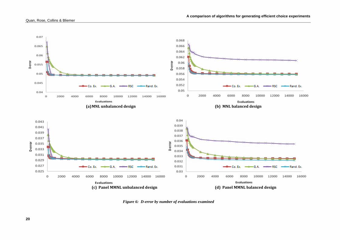
A comparison of algorithms for generating efficient choice experiments Quan, Rose, Collins & Bliemer
20
(a) MNL unbalanced design (b) MNL balanced design
(c) Panel MMNL unbalanced design (d) Panel MMNL balanced design
Figure 6: D-error by number of evaluations examined
A comparison of algorithms for generating efficient choice experiments Quan, Rose, Collins & Bliemer
21
best design. The modified Fedorov algorithm appears to perform somewhere between the coordinate exchange and random exchange algorithms and the genetic algorithm in terms of the number of evaluations required. For balanced designs, a similar pattern exists, where the coordinate exchange and random exchange algorithms tend to locate the most efficient design very quickly whilst the RSC algorithm performs very poorly relative to the other algorithms examined herein.
5.2 Case study 2 The second case study involves the generation of an experiment involving three alternatives, one of which represents a no choice alternative. The two non-no choice alternatives are represented by five attributes. The attribute levels of the design are 1,3,5,7 for the first attribute, 0,0.25,0.5,0.75 for the second attribute, and 0.5,0.6,0.7,0.8, 1,0 and 20,40,60,80 for the third, fourth and fifth attributes respectively. Sixteen choice tasks are generated. The utility specifications for the design are given as Equation (16).
0 1 1 2 2 3 2 4 4 5 51,3,5,7 0,0.25,0.5,0.75 0.5,0.6,0.7,0.8 0,1 20,40,60,80
0 1 1 2 2 3 2 4 4 5 51,3,5,7 0,0.25,0.5,0.75 0.5,0.6,0.7,0.8 0,1 20,40,60,80
( ) ,
( ) .A A A A A A
B B B B B B
U A x x x x x
U B x x x x x
β β β β β β
β β β β β β
= + + + + +
= + + + + + (16)
The two non-no choice alternatives are assumed to have fixed alternative specific constant terms equal to 0 9Aβ = − for alternative one and 0 9.2Bβ = − for alternative two. The remaining parameters are assumed to be generic across the two non-no choice alternatives. Both 1β and
2β are assumed to be normally distributed, such that 1 1 1~ ( , )Nβ µ σ and 2 2 2~ ( , )Nβ µ σ while the remaining priors are assumed to be fixed parameter values. The following prior values are assumed; 3.11 =µ , 6.01 =σ , 52 =µ , 0.22 =σ , 7.23 =β , 34 =β and 015.05 −=β . Gaussian quadrature with 6 abscissas is used for the EV1 error terms in the utility functions, and a sample of 1000 respondents is generated for computing the panel MMNL results.
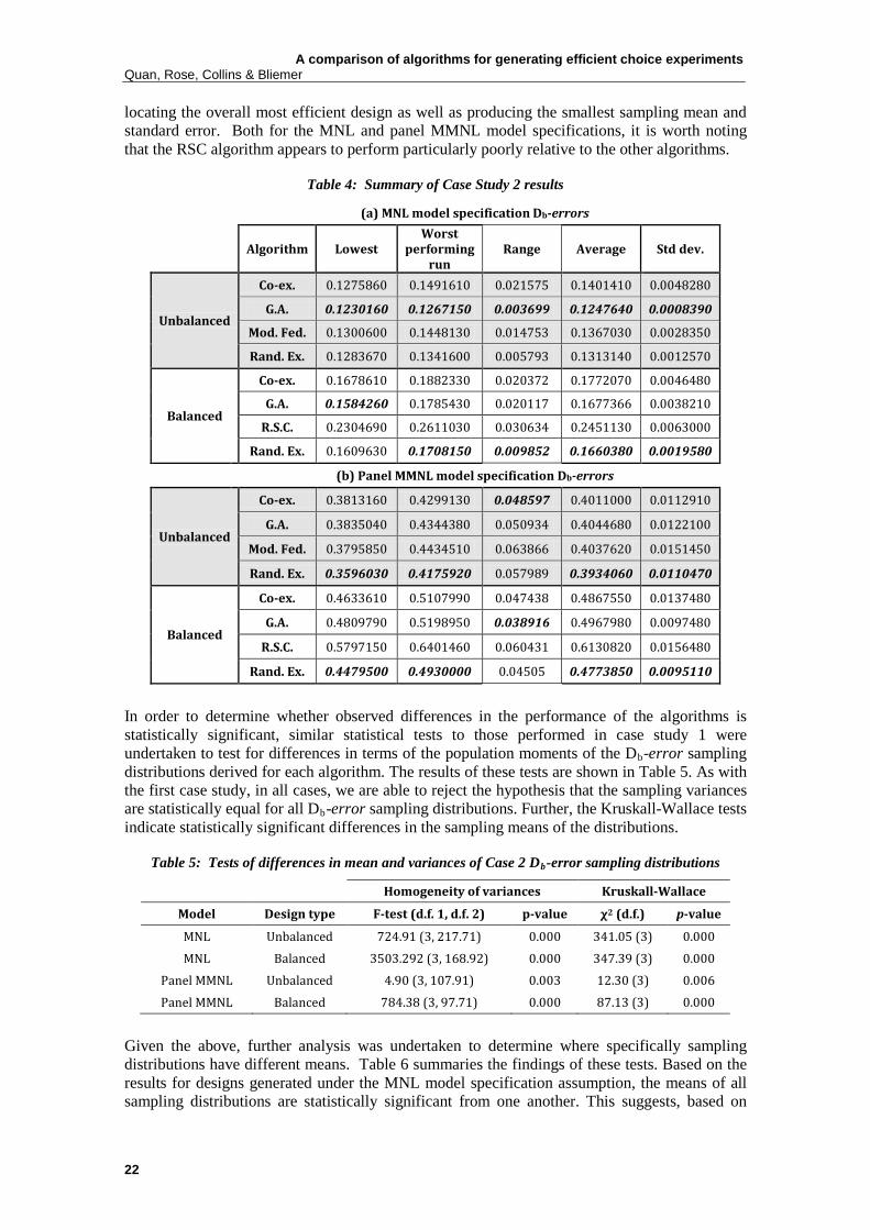
Table 4 provides summary statics for the second case study similar to those presented in Table 1 for case study 1. Given that the design dimensionality explored is much larger than that examined in case study 1, we are unable to compute the optimal D-error for any of the designs in case study 2 as the number of potential designs that need to be explored is too large (there are 48 ×22 = 262,144 possible choice tasks, from which 16 choice tasks can be chosen giving a total of 4.97096 × 1086 possible designs). As such, all comparisons made between the algorithms must be relative to the other algorithms as opposed to some ideal design. From the table, examining the designs generated under an MNL specification assumption and letting go of attribute level balance, the genetic algorithm appears to offer the best performance, locating the most efficient design found for any of the algorithms as well as producing the smallest Db-error sampling average. The genetic algorithm also appears to be the most consistent algorithm. When attribute level balance was imposed, the genetic algorithm was also able to locate the most efficient design found, however the random exchange algorithm provided a lower Db
For the panel MMNL model without attribute balance, the random exchange algorithm appears to outperform the other algorithms in its ability to locate the most efficient design. Further, the algorithm appears to provide the smallest sampling average over the 30 runs as well as the smallest sampling standard error. Nevertheless, the coordinate exchange and genetic algorithms appear to provide more consistency in the D
-error sampling average and standard error suggesting that this algorithm tended to perform better than the coordinate exchange algorithm on average as well as being more consistent. When attribute level balance is maintained as a design criteria, the genetic algorithm was once more able to locate the overall most efficient design, however the random exchange algorithm was found to outperform all other algorithms based on all other criteria examined.
b-error values of the designs located, as based on the range of Db-error values found, even if they perform worse on average. When attribute level balance is maintained, a similar pattern appears in terms of the random exchange algorithm
A comparison of algorithms for generating efficient choice experiments Quan, Rose, Collins & Bliemer
22
locating the overall most efficient design as well as producing the smallest sampling mean and standard error. Both for the MNL and panel MMNL model specifications, it is worth noting that the RSC algorithm appears to perform particularly poorly relative to the other algorithms.
Table 4: Summary of Case Study 2 results
(a) MNL model specification Db-errors
Algorithm Lowest
Worst performing
run Range Average Std dev.
Unbalanced
Co-ex. 0.1275860 0.1491610 0.021575 0.1401410 0.0048280
G.A. 0.1230160 0.1267150 0.003699 0.1247640 0.0008390
Mod. Fed. 0.1300600 0.1448130 0.014753 0.1367030 0.0028350
Rand. Ex. 0.1283670 0.1341600 0.005793 0.1313140 0.0012570
Balanced
Co-ex. 0.1678610 0.1882330 0.020372 0.1772070 0.0046480
G.A. 0.1584260 0.1785430 0.020117 0.1677366 0.0038210
R.S.C. 0.2304690 0.2611030 0.030634 0.2451130 0.0063000
Rand. Ex. 0.1609630 0.1708150 0.009852 0.1660380 0.0019580
(b) Panel MMNL model specification Db-errors
Unbalanced
Co-ex. 0.3813160 0.4299130 0.048597 0.4011000 0.0112910
G.A. 0.3835040 0.4344380 0.050934 0.4044680 0.0122100
Mod. Fed. 0.3795850 0.4434510 0.063866 0.4037620 0.0151450
Rand. Ex. 0.3596030 0.4175920 0.057989 0.3934060 0.0110470
Balanced
Co-ex. 0.4633610 0.5107990 0.047438 0.4867550 0.0137480
G.A. 0.4809790 0.5198950 0.038916 0.4967980 0.0097480
R.S.C. 0.5797150 0.6401460 0.060431 0.6130820 0.0156480
Rand. Ex. 0.4479500 0.4930000 0.04505 0.4773850 0.0095110
In order to determine whether observed differences in the performance of the algorithms is statistically significant, similar statistical tests to those performed in case study 1 were undertaken to test for differences in terms of the population moments of the Db-error sampling distributions derived for each algorithm. The results of these tests are shown in Table 5. As with the first case study, in all cases, we are able to reject the hypothesis that the sampling variances are statistically equal for all Db
Table 5: Tests of differences in mean and variances of Case 2 D
-error sampling distributions. Further, the Kruskall-Wallace tests indicate statistically significant differences in the sampling means of the distributions.
b
-error sampling distributions
Homogeneity of variances Kruskall-Wallace
Model Design type F-test (d.f. 1, d.f. 2) p-value χ2 (d.f.) p-value
MNL Unbalanced 724.91 (3, 217.71) 0.000 341.05 (3) 0.000 MNL Balanced 3503.292 (3, 168.92) 0.000 347.39 (3) 0.000
Panel MMNL Unbalanced 4.90 (3, 107.91) 0.003 12.30 (3) 0.006 Panel MMNL Balanced 784.38 (3, 97.71) 0.000 87.13 (3) 0.000
Given the above, further analysis was undertaken to determine where specifically sampling distributions have different means. Table 6 summaries the findings of these tests. Based on the results for designs generated under the MNL model specification assumption, the means of all sampling distributions are statistically significant from one another. This suggests, based on

A comparison of algorithms for generating efficient choice experiments Quan, Rose, Collins & Bliemer
23
Table 4, that for the unbalanced design, the modified Fedorov algorithm is statistically more likely to locate more efficient designs than the other algorithms whilst for attribute level balanced designs, the random exchange algorithm performs best on average. For designs constructed for the panel MMNL model specification, the mean of the Db
Table 6: Summary of results obtained from Games-Howell statistical tests for Case 2
-error sampling distribution associated with the random exchange algorithm is statistically different to that obtained from all other algorithms both when attribute level balance is maintained or relaxed. Combined with information from Table 4, this suggests that the random exchange algorithm is statistically more likely to locate more efficient designs than the other algorithms under the panel MMNL specification model assumption.
Model Design type Note MNL Unbalanced All sampling means different at p = 0.05 level of significance MNL Balanced All sampling means different at p = 0.05 level of significance
Panel MMNL Unbalanced Cannot reject Co. Ex., G.A. And Mod Fed. sampling means different (p >0.658); Rand. Ex. sampling mean different to others at p = 0.05 level of significance
Panel MMNL Balanced All sampling means different at p = 0.05 level of significance
Although not reported, plots similar to Figure 6 were also generated for the second case study. These Figures are not shown here as they mirror those of the first case study where the coordinate exchange and random exchange algorithms tend to locate very quickly quite efficient designs whilst the genetic algorithm tends to require many more evaluations to locate the best design. The RSC algorithm stands out once more as requiring many more evaluations to locate more efficient designs, never approaching the Db
6. Discussion and conclusion
-error values of the other algorithms.
In this paper, we have examined the performance of a number of algorithms for generating efficient designs under different assumptions, namely assumptions about attribute level balance as well as about model types, in particular the MNL and panel MMNL model specifications. In doing so, we have not only compared and contrasted the performance of already existing and implemented algorithms, but also a number of new algorithms. Examined were the previously implemented modified Fedorov, RSC and coordinate exchange algorithms. Contrasted to these were two algorithms new to the generation of SC experiments, introduced here for the first time. These included a genetic algorithm and relatively simple algorithm we have termed the random exchange algorithm.
Our results suggest that within the class of problems examined herein, the genetic algorithm did not perform as well as was expected. Whilst the genetic algorithm performed particularly well for the unlabeled case in the second case study, the other algorithms, whilst producing slightly worse designs in terms of statistical efficiency, still tended to locate acceptable designs and in doing so, used many less evaluations than the genetic algorithm. Further, the RSC and modified Fedorov algorithms appear to perform relatively poorly when compared to other possible algorithms, despite dominating the literature in terms of their usage. Based on two simulated case studies, it would appear that the random exchange algorithm tends to offer performance advantages over all other algorithms examined, both when attribute level balance is applied or not and for both the MNL and panel MMNL model specifications. Whilst the algorithm does not dominate on all criteria, an examination of the results suggests that the random exchange algorithm appears to locate very quickly relatively efficient designs, requiring few design evaluations to do so. Further, the random exchange algorithm appears to locate designs with lower Db-errors than the other algorithms examined, and in doing so, locate more efficient designs more consistently than the other algorithms. These are desirable properties to the

A comparison of algorithms for generating efficient choice experiments Quan, Rose, Collins & Bliemer
24
practitioner, who may have only limited time to search for a design, and who will likely value not having to perform multiple searches to overcome sampling variability.
It is worth noting that it may be possible in the future to design improved algorithms than examined herein. Presently, the algorithms examined here and used elsewhere in the literature rely on a brute strength approach, comparing all, or as many as is practical, possible attribute level combinations. Research examining the efficiency measures assumed to compare different experimental designs however have shown in specific cases information that may be useful when considering the next generation of algorithms for generating efficient SC experimental designs. For example, Kanninen (2002) and Toner et al. (1999) have shown that in the case of binary choice experiments under the assumption of non-zero local priors, that there exist particular sets of choice probabilities that when obtained, result in the most optimal design possible. Given this information, it may be possible in the future to implement algorithms that concentrate on choice tasks that produce choice probabilities that deviate from the known desirable values. In this way, such algorithms may be able to able to target specific choice tasks, making changes only to those where improvements are likely to occur. Additionally, improvements to the algorithms examined herein may be possible. For example, if attribute level balance is not required, a genetic algorithm in which the cross-over is based on rows instead of columns should be considered. This way, the algorithm maintains the ‘good’ choice tasks as genes in the population. Further, crossing over rows as opposed to columns may improve the speed of the algorithm for the MNL and cross-sectional MMNL model specifications, as only the Fisher information of the affected choice tasks need be directly calculated without any new computations for the other choice tasks required (see Kessels et al. 2009). This advantage is not available to the genetic algorithm approach adopted here involving column cross-over, where there is a need to re-evaluate the complete design. As such, it is possible that future research examine algorithms for specific problems where they may be tailored specifically to provide the best results, both in terms of speed and the ability to locate more efficient designs, rather than the current approach of adopting a one-size fits all approach to the problem.
This paper also suffers from a number of limitations that need to be acknowledged. Firstly, we have employed here only two case studies. As such, the results presented herein are specific to the case studies examined and do not allow for a detailed analysis of the impact different design dimensions might play beyond those altered herein. As such, we are unable to determine for example whether the results hold if the number of alternatives increases beyond what has been assumed in both case studies. Similarly, questions such whether having more or less choice situations will impact upon the performance of the various algorithms cannot be answered. As such, we suggest further research into the impact that design dimensionality plays on the performance of the various algorithms. We note that such questions are particularly relevant for practitioners where time allocated to generating SC experiments may be limited.
Secondly, in our analysis, we have limited our examination to designs which did not impose any restrictions on dominance or other restrictions on what combinations of attribute levels are allowed in the design. In terms of dominance, a cursory examination of many of the published papers dealing with efficient designs will reveal that many of choice tasks generated have dominated alternatives. Whilst in theory, such choice tasks may result in greater statistical efficiency, typically in practice such choice tasks should be avoided. As such, future research may wish to examine the performance of various algorithms when dominated alternatives are prevented from entering into the design. Likewise, many practical examples exist where certain attribute level combinations are undesirable and hence are restricted from being allowed to occur within a design. The case studies presented herein did not provide any such constraints and as such may be somewhat removed from the types of designs that practitioners may wish to generate for empirical settings. Quite clearly, the imposition of such constraints will impact upon the performance of the various algorithms where for example, the candidate set of the modified Fedorov algorithm can be tailored to remove alternatives with undesirable attribute level combinations in advance or alternatively, the candidate set could be constructed to

A comparison of algorithms for generating efficient choice experiments Quan, Rose, Collins & Bliemer
25
constitute entire choice tasks as opposed to single alternatives, in which case choice tasks with dominated alternatives could also easily be removed. As such, future research should consider such constraints when exploring similar lines of enquiry.
References
Anderson, D.A. and Wiley, J.B. (1992) Efficient Choice Set Designs for Estimating Cross-Effects Models, Marketing letters, 3(4), 357-370.
Bliemer, M.C.J. and Rose, J.M. (2011) Experimental design influences on stated choice outputs: an empirical study in air travel choice, Transportation Research Part A, 45(1), 63-79.
Bliemer, M.C.J. and Rose, J.M. (2010) Construction of Experimental Designs for Mixed Logit Models Allowing for Correlation Across Choice Observations, Transportation Research Part B, 46(3), 720-734.
Bliemer, M.C.J. and Rose, J.M. (2009) Designing Stated Choice Experiments: The state of the Art, in Kitamura, R., Yoshi, T. and Yamamoto, T. (eds.), The Expanding Sphere of Travel Behaviour Research, Selected Papers from the 11th
Bliemer, M.C.J., Rose, J.M. and Hess, S. (2008) Approximation of Bayesian Efficiency in Experimental Choice Designs, Journal of Choice Modelling, 1(1), 98-127.
International Conference on Travel Behaviour Research, Ch25, 495-498.
Brown, M.B. and Forsythe, A.B. (1974) Robust tests for equality of variances, Journal of American Statistical Association, 69, 264-267.
Burgess, L. and Street, D.J. (2005) Optimal designs for choice experiments with asymmetric attributes, Journal of Statistical Planning and Inference, 134, 288-301.
Carlsson, F. and Martinsson, P. (2002) Design Techniques for Stated Preference Methods in Health Economics, Health Economics, 12, 281-294.
Chaloner, K. and Verdinelli. I. (1995) Bayesian Experimental Design: A Review, Statistical Science, 10(3), 273–304.
Cook, D.R. and Nachtsheim, C.J. (1980) A Comparison of Algorithms for Constructing Exact D-Optimal Designs, Technometrics, 22(3), 315–24.
Fedorov, V.V. (1972) Theory of Optimal Experiments, New York: Academic Press.
Games, P.A. and Howell, J.F. (1976) Pairwise Multiple Comparison Procedures with Unequal N's and/or Variances: A Monte Carlo Study, Journal of Educational Statistics, 1, 113-125.
Goegebeur, Y., Goos, P. and Vandeboek, M. (2007) A hierarchical Bayesian approach to robust parameter design, Department of decision sciences and information management working paper, 0719.
Grossmann, H., Holling, H. and Schwabe, R. (2002) Advances in Optimum Experimental Design for Conjoint Analysis and Discrete Choice Models, in Franses, P.H. and Montgomery, A.L. (eds.) Advances in Econometrics, Econometric Models in Marketing, 16, Amsterdam: JAI Press, 93–117.

A comparison of algorithms for generating efficient choice experiments Quan, Rose, Collins & Bliemer
26
Hedayat, A.S., Sloane, N.J.A. and Stufken, J. (1999) Orthogonal Arrays: Theory and Applications, Springer Verlag, New York.
Heredia-Langner, A. Carlyle, W.M., Montgomery, D.C, Borror, C.M. and Runger, G.C. (2003) Genetic algorithms for the construction of D-optimal Designs, Journal of Quality Technology, 35(1), 28-46.
Huber, J. and Zwerina, K. (1996) The Importance of utility Balance and Efficient Choice Designs, Journal of Marketing Research, 33, 307-317.
Kanninen, B.J. (2002) Optimal Design for Multinomial Choice Experiments, Journal of Marketing Research, 39(2), 214-217.
Keselman, H.J. and Rogan, J.C. (1978) A Comparison of the Modified-Tukey and Scheffe Methods of Multiple Comparisons forPairwise Contrasts, Journal of the American Statistical Association, 73(361), 47-52.
Kessels, R., Bradley, B. Goos, P. and Vandebroek, M. (2009) An Efficient Algorithm for Constructing Bayesian Optimal Choice Designs, Journal of Business and Economic Statistics, 27(2), 279-291.
Kessels, R., Goos, P., and Vandebroek, M. (2006) A comparison of criteria to design efficient choice experiments, Journal of Marketing Research, 43(3), 409-419.
Kuhfeld, W. F., and Tobias, R.D. (2005) Large factorial designs for product engineering and marketing research applications, Technometrics, 47(2), 132-141.
Kuhfeld, W.F., Tobias, R.D. and Garratt, M. (1994) Efficient experimental design with marketing research applications, Journal of Marketing Research, 31(4), 545-557.
Lazari, A.G. and Anderson, D.A. (1994) Designs of discrete choice set experiments for estimating both attribute and availability cross effects, Journal of Marketing Research, 31(3), 375-383
Louviere, J.J., Hensher, D.A. and Swait, J.D. (2000) Stated Choice Methods: Analysis and Application, Cambridge University Press, Cambridge.
Louviere, J.J., Islam, T., Wasi, N., Street, D. and Burgess, L. (2008) Designing Discrete Choice Experiments: Do Optimal Designs Come at a Price? Journal of Consumer Research, 35(2), 360-375.
Meyer, R.K., and Nachtsheim, C.J. (1995) The coordinate-exchange algorithm for constructing exact optimal experimental designs, Technometrics, 37(1), 60-69.
Poland, J. Mitterer, A. Knödler, K. and Zell, A. (2001) Genetic algorithms can improve the construction of D-optimal experimental designs, in Mastorakis, N. (ed.) Advances in Fuzzy Systems and Evolutionary Computation, World Scientific Engineering Society, Puerto de la Cruz, Spain 227-231.
Rose, J.M. and Bliemer, M.C.J. (2009) Constructing Efficient Stated Choice Experimental Designs, Transport Reviews, 29(5), 587-617.
Sándor, Z., and M. Wedel (2005) Heterogeneous conjoint choice designs, Journal of Marketing Research, 42, 210-218.

A comparison of algorithms for generating efficient choice experiments Quan, Rose, Collins & Bliemer
27
Sándor, Z., and M. Wedel (2002) Profile Construction in Experimental Choice Designs for Mixed Logit Models, Marketing Science, 21(4), 455-475.
Sándor, Z., and M. Wedel (2001) Designing Conjoint Choice Experiments Using Managers’ Prior Beliefs, Journal of Marketing Research, 38, 430-444.
Siegel, S. and Castellan, N. (1988) Nonparametric Statistics for the Behavioral Sciences, McGraw Hill, New York.
Street, D.J., and L. Burgess (2004) Optimal and Near Optimal Pairs for the Estimation of Effects in 2-Level Choice Experiments, Journal of Statistical Planning and Inference, 118 (1–2), 185–99.
Street, D.J., L. Burgess, and J.J. Louviere (2005) Quick and Easy Choice Sets: Constructing Optimal and Nearly Optimal Stated Choice Experiments, International Journal of Research in Marketing, 22, 459-470.
Toner, J.P., S.D., Clark, S.M., Grant-Muller and A.S. Fowkes (1999) Anything you can do, we can do better: a provocative introduction to a new approach to stated preference design, WCTR Proceedings, 3, Antwerp, 107-120.
Vermeulen, B., P. Goos and M. Vandeboek (2008) Models and optimal designs for conjoint choice experiments including a no-choice option, International Journal of Research in Marketing, 25(2), 94-103.
Yu, J., Goos, P. and Vandeboek, M. (2010) Comparing different sampling schemes for approximating the integrals involved in the semi-Bayesian optimal design of choice experiments, Department of decision sciences and information management working paper, 0827.
Yu, J., Goos, P.P. and Vandebroek, M. (2009) Efficient conjoint choice designs in the presence of respondent heterogeneity, Marketing Science, 28, 122-135.
Yu, J., Goos, P. and Vandeboek, M. (2008) A Comparison of Different Bayesian Design Criteria to Compute Efficient Conjoint Choice Experiments, Department of decision sciences and information management working paper, 0817.