5757 S. University Ave.

Chicago, IL 60637

Main: 773.702.5599

bfi.uchicago.edu

WORKING PAPER · NO. 2020-72

Epidemic Responses Under UncertaintyMichael Barnett, Greg Buchak, and Constantine YannelisMAY 2020

Epidemic Responses Under Uncertainty∗

Michael Barnett

Arizona State University

W.P. Carey School of Business

Greg Buchak

Stanford University

Graduate School of Business

Constantine Yannelis

University of Chicago

Booth School of Business

May 2020

Abstract

We examine how policymakers should react to a pandemic when there is signif-

icant uncertainty regarding key parameters relating to the disease. In particular,

this paper explores how optimal mitigation policies change when incorporating un-

certainty regarding the Case Fatality Rate (CFR) and the Basic Reproduction Rate

(R0) into a macroeconomic SIR model in a robust control framework. This paper

finds that optimal policy under parameter uncertainty generates an asymmetric op-

timal mitigation response across different scenarios: when the disease’s severity is

initially underestimated the planner increases mitigation to nearly approximate the

optimal response based on the true model, and when the disease’s severity is initially

overestimated the planner maintains lower mitigation as if there is no uncertainty in

order to limit excess economic costs.

JEL: E1, H0, I1

Keywords: COVID-19, Coronavirus, Model Uncertainty, Dynamic General Equilibrium

∗We are grateful to Scott Baker, Nick Bloom, Buz Brock and Lars Hansen for helpful comments anddiscussions. This draft is preliminary and incomplete, comments are welcome.

1 Introduction

The rapid spread of COVID-19 in 2020 was accompanied by a vigorous debate about the

costs and benefits of severe actions taken to mitigate the spread of the pandemic. This

debate was conducted with significant uncertainty about key parameters relating to the

costs of the new virus, including death rates, infection rates and the economic costs of

policies such as shuttering businesses and issuing shelter-in-place orders (Chater, 2020)1.

Many policymakers and commentators in the media used the fact that there was significant

uncertainty about the effects of COVID-19 to argue that this should lead to a more lax

policy response, keeping businesses open and allowing free movement.2 It is far from

obvious, however, how uncertainty regarding the fundamentals of a potential threat should

alter the optimal policy response. This paper explores how the economic and public health

consequences of pandemic mitigation policies should be assessed in the face of significant

uncertainty.

Determining the optimal response to COVID-19 is a prime example of policy makers

having to make decisions with significant amounts of uncertainty. Even several months into

the pandemic, there remained significant disagreement regarding key parameters relating to

the damages of the new virus. In Epidemiology, two factors are particularly important for

evaluating the severity of a contagious disease: first, the Case Fatality Rate (CFR), or the

fraction of individuals infected who die due to the disease; second, the basic reproduction

numberR0, or the number of people in an otherwise healthy population that a single disease

carrier is expected to infect. For example, estimates of the CFR ranged from being close to

that of the seasonal flu, to two orders of magnitude higher than a seasonal flu. Estimates

of R0 varied widely due to difficulty in measuring how many people were infected, in part

due to the presence of a large number of asymptomatic carriers.3 This uncertainty made it

difficult for policy makers to weigh the health benefits of policies such as lockdowns against

1Early estimates of the Case-Fatality Rate (CFR) ranged from .08% to 13.04%. Estimates of the numberof individuals each carrier infects, R0, ranged from 1.5 to 12 (Korolev, 2020)

2For example, the Mayor of New York Bill De Blasio noted in a March 9 press conference when askedwhether the city would cancel a St. Patrick’s day parade that “I am very resistant to take actions thatwe’re not certain would be helpful, but that would cause people to lose their livelihoods.”

3The wide range of estimates is discussed in Manski and Molinari (2020) who derive bounds for param-eters: “In the present absence of random testing, various researchers have put forward point estimates andforecasts for infection rates and rates of severe illness derived in various ways... The assumptions varysubstantially and so do the reported findings... We find that the infection rate as of April 6, 2020, forIllinois, New York, and Italy are, respectively, bounded in the intervals [0.001, 0.517], [0.008, 0.645], and[0.003, 0.510].”

1

their economic damages.

The uncertainty about the effects of the virus on health outcomes has led some policy-

makers to suggest taking less severe steps to stem the spread of the virus. This sentiment

was expressed by the well-known epidemiologist John Ioannides who noted in a widely-read

opinion piece saying that

“In the absence of data, prepare-for-the-worst reasoning leads to extreme mea-

sures of social distancing and lockdowns. Unfortunately, we do not know if these

measures work.... This has been the perspective behind the different stance of the

United Kingdom keeping schools open, at least until as I write this. In the absence

of data on the real course of the epidemic, we don’t know whether this perspective

was brilliant or catastrophic.”

Despite this and similar commentary from some policymakers suggesting that signifi-

cant uncertainty should prevent drastic measures from being taken, economic theory would

in fact suggest that the opposite conclusion is true. Higher levels of uncertainty should

lead policymakers to avoid large losses, adopting a “maxmin” criterion (Hansen and Sar-

gent, 2001) by selecting the policy that would be optimal under the worst-case scenario.

Of course, the selection of the worst-case scenario itself must be disciplined by what is

reasonably consistent with the data: For example, an extremely contagious disease with

an eventual 100% fatality rate is indeed a worst-case scenario, but—parameter uncertainty

notwithstanding—is not consistent with even the most pessimistic estimates. A CFR of

10%, however, while towards the extreme end of estimates, may be a reasonable worst-case

scenario to consider. In this paper, we examine the smooth ambiguity and robust control

approaches, which provide analytical frameworks to select a reasonable worst-case scenario

to inform optimal policy decisions.

We embed parameter uncertainty into a simple macroeconomic model featuring a pan-

demic. In the model, policy-makers must weigh the health benefits of quarantine against

economic damages inflicted by these policies. We begin with a standard Susceptible, In-

fectious, or Recovered4 (SIR) model augmented by Brownian motions. These Brownian

shocks capture not only randomness in the spread of the disease, but importantly, difficul-

ties in measuring infections and classifying deaths. These perturbations make it difficult

4SIR models are standard tools in epidemiology used to model the spread of infectious diseases. Theepidemiological SIR model computes the theoretical number of people infected with a contagious diseasein a closed population over time. The models have three key elements: S is the number of susceptible, Iis the number of infectious, and R is the number of recovered, deceased, or immune individuals. A recentliterature in macroeconomics incorporates SIR models into macroeconomics models. Stanford Earth SystemSciences notes provide a introduction to the standard epidemiological SIR model.

2

for a policy maker to infer the true parameter values underlying the disease’s spread and

case severity, meaning that the policy maker must make policy decisions knowing that her

model is ambiguously specified or potentially misspecified. We compare optimal policies as

well as public health and economic outcomes in a model that explicitly takes this poten-

tial ambiguity or misspecification into account. We calibrate the model to match the US

economy, and explore how uncertainty influences optimal quarantine policy.

We find that more uncertainty about parameters of a disease—death rates and re-

production rates—leads a policy maker to optimally adopt a harsher quarantine in most

situations. This is particularly true when the policy maker’s initial prior on the disease’s

severity is low and it is allowed to spread. As relatively large portions of the population

become infected, the cost of underestimating the disease increases. This is because in a

worst-case scenario, the pool of already-infected people will lead to significantly more in-

fections and death than if the pool of potential spreaders was much smaller. Thus, when

there is more uncertainty about the impact of a new virus, the government should do more

to combat the spread. The intuition for this finding is that the planner seeks to avoid the

worst possible outcomes, in case the uncertainty resolves in an adverse way.

There is an economically important asymmetry that we find when the policy maker’s

initial prior on the disease’s severity is high. Because far smaller portions of the population

become infected than the prior model would expect, the cost of underestimating the disease

decreases. The planner views potential outcomes under the worst-case model to be far

less adverse than they might have otherwise. As a result, the planner acts as if there

is essentially no uncertainty about the impact of a new virus and chooses an optimal

quarantine strategy accordingly. This key finding demonstrates that not only does choosing

optimal policy under uncertainty lead to important increases in quarantine in the case that

the virus has been underestimated, but also that excess economic costs from high levels of

quarantine are now worse than when choosing optimal policy as if there was no uncertainty.

This paper links to a literature on robust control beginning with Hansen and Sargent

(2001). Detailed explanations of robust preference problems and axiomatic treatment of

such formulations using penalization methods are given by Anderson, Hansen, and Sar-

gent (2000), Hansen, Sargent, Turmuhambetova, and Williams (2001), Cagetti, Hansen,

Sargent, and Williams (2002), Anderson, Hansen, and Sargent (2003), Hansen, Sargent,

Turmuhambetova, and Williams (2006), Maccheroni, Marinacci, and Rustichini (2006),

and Hansen and Sargent (2011). The paper also relates to a literature on dealing with

policy uncertainty, for example Bloom (2009) and Baker, Bloom, and Davis (2016).

3

We apply tools developed to the economic costs of climate change, given model un-

certainty regarding the projected effects of climate change. Much research has focused on

determining whether the impacts of climate change are temporary damages on the level of

output, or more permanent damages on the growth rate of output (see Dell, Jones, and

Olken (2012), Colacito, Hoffmann, and Phan (2018), Hsiang, Kopp, Jina, Rising, Delgado,

Mohan, Rasmussen, Muir-Wood, Wilson, Oppenheimer, et al. (2017), Baldauf, Garlappi,

and Yannelis (2019) and Burke, Davis, and Diffenbaugh (2018) for examples focused on

empirically estimating these different types of climate damages). Level effects can lead to

very different choices by social planners in terms of choices about emissions and carbon

mitigation in a climate economic setting compared to growth effects (see Hambel, Kraft,

and Schwartz (2015) and Barnett, Brock, and Hansen (2020) for theoretical examples show-

ing how these different types of damages can lead to very different social costs of carbon

results). However, in our pandemic setting the planner is able to use optimal policy to de-

termine whether to subject the economy to quarantine measures that produce short-term

damages or larger long-term damages that are partially discounted. This is the key effect

driving the planner’s optimal decision. The role that model uncertainty plays is amplifying

concerns about the worst case outcomes, that infection and death rates are potentially

much higher and thus the permanent effects could be much worse. As a result, the planner

shifts more weight to the possibility of larger permanent, long-term costs coming from in-

creased deaths and as a result increases current, short-term costs from quarantine measures

in a dynamic model.

The paper introduces uncertainty to the discussion on economic responses to the COVID-

19 epidemic. A number of studies have built macroeconomic frameworks, combining SIR

models from epidemiology with macroeconomic models, such as Kaplan, Moll, and Vi-

olante (2020), Jones, Philippon, and Venkateswaran (2020), Baker, Bloom, Davis, and

Terry (2020) and Eichenbaum, Rebelo, and Trabandt (2020). These studies rely on cal-

ibrated parameters, which are often unknown. Parameter uncertainty is widely noted

in this literature, and authors typically use a range of values. For example, Acemoglu,

Chernozhukov, Werning, and Whinston (2020) note that: “We stress that there is much

uncertainty about many of the key parameters for COVID19 (Manski and Molinari, 2020)

and any optimal policy, whether uniform or not, will be highly sensitive to these parameters

(e.g., Atkeson (2020a), Avery, Bossert, Clark, Ellison, and Ellison (2020), Stock (2020)).

So our quantitative results are mainly illustrative and should be interpreted with caution.”

Our paper offers a framework for incorporating uncertainty explicitly in a wide class of

4

macroeconomics models.

Other studies have studied the impact of the COVID-19 epidemic on household con-

sumption (Baker, Farrokhnia, Meyer, Pagel, and Yannelis, 2020a,b), social distancing (Bar-

rios and Hochberg, 2020, Allcott, Boxell, Conway, Gentzkow, Thaler, and Yang, 2020), la-

bor markets (Coibion, Gorodnichenko, and Weber, 2020), small business Granja, Makridis,

Yannelis, and Zwick (2020) and inequities (Coven and Gupta, 2020). Some papers also

focus on estimating damages. Using historical data from the Spanish flu, Barro, Ursua,

and Weng (2020) argue for an upper bound of between 6 and 8 percent of GDP for the

impact of the virus. Gormsen and Koijen (2020) argue that stock market reactions imply

an approximate 2 to 3 percent change in GDP growth.

The remainder of this paper is organized as follows. Section 2 discusses uncertainty.

Section 3 presents our model. Section 4 describes how to account for uncertainty. Section 5

presents simulation results. Section 6 discusses model extensions and section 7 concludes.

2 Uncertainty and Pandemics

We differentiate three aspects of uncertainty following Knight (1971) and Arrow (1951),

and discuss how they are best understood in the context of an epidemic.

1. Risk refers to outcomes within a model where probabilities are known.5 For example,

by going to work, there is a risk that an individual catches the disease; once infected,

there is a risk that the individual dies. These risks are present regardless of our

knowledge of the parameters underlying the pandemic.

2. Ambiguity, refers to uncertainty across models, where, for example, a researcher

or policy maker does not know how much weight to assign to one model as opposed

to another. For example, from the perspective of a policymaker, a new disease may

have a mild CFR or it may have a high CFR, and the policymaker does not know

how much weight to assign one model versus another.

3. Misspecification or model uncertainty refers to uncertainty about models, or flaws

in models not known to researchers. For example, from the perspective of a poli-

5A large literature refers to this risk as uncertainty, for example Bloom (2009) and Baker, Bloom, andDavis (2016). To avoid confusion, we use the terms risk to denote a situation where probabilities are knownand ambiguity to refer to a situation where probabilities are unknown.

5

cymaker there is a range of plausible CFRs for a new disease, and the policymaker

worries that the CFR used to form policy decisions may be misspecified.

In the context of COVID-19, there was significant uncertainty regarding its overall

effects in early 2020 (Chater, 2020), relating to risk, ambiguity and misspecification. It

is understood that it is risky to expose oneself to the disease, and at a high level, the

SIR model captures important aspects of pandemic spread. However, whether a healthy

person coming in contact with an infected person has a 1% or 10% chance of contracting

the disease, and whether an infected person has a 0.1% or 10% chance of dying, is critical

in shaping policy yet unknown to policymakers. Our approach in this paper is to explicitly

model optimal policymaker decision rules under potential model misspecification, focusing

on the CFR and R0 of the disease.

Figure 1: Estimated CFR Rates by Country

0.0

5.1

.15

CFR

Feb 29 Mar 15 Mar 31Date

0.0

5.1

.15

CFR

Feb 29 Mar 15 Mar 31Date

China USGermany FranceItaly SpainIran UK

Notes: This figure shows estimated CFR rates for all countries with more than 1,000 cases and 100 deaths.Source: European Centre for Disease Prevention and Control.

6

First, there were significant differences in estimates of the CFR across countries. For

example, in Italy the CFR as 12.67%, while in Germany the CFR was 2.07%– an approxi-

mate sixfold difference. Figure 1 shows CFR rates by country between March 1 and April

9, 2020 during the early spread of the pandemic in Europe and the United States. The

eight countries with the largest number of COVID-19 cases at the time are highlighted.

While several countries estimate CFR rates above 10%, some estimates put the CFR as

being as low at .1%. Estimating a CFR for a new disease while cases are ongoing is inher-

ently difficult, as cases must be closed through either recovery or death before a CFR can

be computed (Spychalski, B lazynska-Spychalska, and Kobiela, 2020). Additionally, many

countries have very different reporting and testing practices, making it difficult to estimate

the number of confirmed cases and deaths due to COVID-19 versus other causes.

Figure 2: Estimated R0 for Countries and States

05

1015

R0

California France Germany Japan New York Taiwan UK USA

σ=1/3, γ=1/4 σ=1/4, γ=1/10σ=1/5, γ=1/18

This figure shows estimated R0 rates for different countries and states, and different parameters of theincubation period of the disease (σ) and the estimated duration of the illness (γ). Source: Korolev (2020).

7

Second, estimates of the basic reproduction number, R0, varied widely. R0 is the

expected number of new cases generated by a single case in an uninfected population and

a key determinant of the spread of the disease. Estimates ranged from 1.5 to 12 (Korolev,

2020). A key threshhold is whether R0 ž 1: When R0 ą 1, it means that the disease will

spread in the population, because a single infected will spread it to multiple people, who

will then spread it to multiple people, and so on. In contrast, an R0 ă 1 means that the

number of infected people will decrease over time because each infected person will infect

less than one other and will herself eventually recover or die. Figure 2 shows estimates

of the parameter in several states and countries, under different parameterizations of the

incubation period of the illness and duration. This uncertainty about R0 is noted in many

academic papers, for example Stock (2020) notes in a paper on data gaps related to COVID-

19 that “A key parameter, the asymptomatic rate (the fraction of the infected that are not

tested under current guidelines), is not well estimated in the literature because tests for the

coronavirus have been targeted at the sick and vulnerable.”

One key factor regarding uncertainty in both the CFR and R0 was a lack of testing, and

the fact that many cases are initially asymptomatic. This makes it very difficult to ascertain

the true number of individuals infected with COVID-19, and hence determine the CFR

and R0. Many policymakers and academics were well aware of uncertainty surrounding

key determinants of the health costs of COVID-19. For example, the Asian Development

Bank cited a range of parameters of R0 between 1.5 and 3.5, and a CFR between 1% and

3.4%, and notes that these are imprecisely estimated.

In the subsequent analysis, we focus on uncertainty about these two parameters.6 To

do so, we first present a simple economic model of an epidemic without uncertainty. Here,

the central planner has full knowledge of the virus’s R0 and CFR, and chooses an optimal

quarantine policy taking into account its future impact on the spread of the virus as well as

the economic costs of quarantine. We then add parameter uncertainty by augmenting the

social planner decision problem using either a smooth ambiguity approach or a robustness

approach to explore how parameter uncertainty impacts the optimal policy.

6It is important to note that there are also other potential, un-modeled health costs. For example,even if the CFR is low, COVID-19 could cause permanent damage to lungs in a fashion similar to SARS, arelated coronavirus. Additionally, in follow-on work we plan to incorporate uncertainty about the economiccosts of mitigation measures.

8

3 A Simple Economic Model of an Epidemic

We first sketch out a simple economic model of an epidemic without model uncertainty. We

then explicitly incorporate model uncertainty in subsequent sections. Our model begins

with a standard Susceptible-Infectious-Recovered (SIR) framework used throughout math-

ematics, medicine, epidemiology, and other fields that study pandemics.7 We augment this

SIR model with an economic model that allows us to speak to the costs of the disease as

well as the costs and benefits of mitigation efforts.

3.1 Epidemic Model

A standard SIR model is characterized by three states: the fraction of the population that

is susceptible to the disease, st, the fraction of the population infected by the disease, it,

and the fraction of the population recovered from infection, rt. We include a fourth state,

death, dt, which tracks the fraction of the population that has died because of the disease.

The size of the population is assumed to be fixed. These states evolve as follows:

dst “ ´βstitdt

dit “ βstitdt´ pρ` δqitdt

drt “ ρitdt

ddt “ δitdt

β is the rate at which a susceptible becomes infected when meeting a an infected. ρ is the

rate at which an infected recovers, and δ is the rate at which an infected dies.

We allow for uncertainty about the SIR model parameters. The key parameters we

focus on are R0, the expected number of secondary cases that a single infection produces

in a fully-susceptible population, and the case fatality rate (CFR), which is the proportion

of deaths relative to the total number of infected. These two parameters, combined with

the expected duration of the disease (γ), link to the key structural disease parameters in

our model, β, ρ, and δ, as follows:

R0 “β

γ, CFR “

δ

γ, γ “ ρ` δ

We allow for uncertainty connected to these two parameters in our model in multiple

7Stanford Earth System Sciences notes provide a basic outline of a standard epidemiological SIR model.

9

ways. First, we introduce Brownian shocks connected to the evolution of it and dt to the

deterministic transition rates above. These shocks capture, among other things, variability

in exposures, variability in the co-morbidities of the affected population, and potential

mismeasurement of the number of infected and dead.

These shocks are critical when we later add parameter uncertainty, because they pre-

vent policy makers from immediately learning about the fundamental transition rates of

the disease. We add these shocks under a few key assumptions: the first shock is per-

fectly negatively correlated between st and it so that shocks to infections only occur in the

susceptible population, which one can interpret as uncertainty over whether an individual

is infected or has never been infected; the second shock is perfectly negatively correlated

between it and dt so that shocks to deaths occur in the infected population; and all shocks

are scaled by it so that when there are no infected individuals there can no longer be shocks

to the number of infected and dead. With these shocks and assumptions, the state variable

evolution becomes:

dst “ ´βstitdt´ σβitdWi

dit “ βstitdt´ pρ` δqitdt` σβitdWi ´ σδitdWd

drt “ ρitdt

ddt “ δitdt` σδitdWd

Formally, W.“ tWt : t ě 0u is a multi-dimensional Brownian motion where the correspond-

ing Brownian filtration is denoted by F .“ tFt : t ě 0u and Ft is generated by the Brownian

motion between dates zero and t. Figure 3 illustrates the transition rates between states

in our model under this risk based framework.

Including Brownian shocks in our model captures the risk channel of uncertainty. How-

ever, key to our analysis will be extending our analysis to account for additional channels

of uncertainty. In our analysis, we will explore the impact of he ambiguity-based channel

of uncertainty and the misspecification-based channel of uncertainty, which we explicitly

model in later sections of the paper.

10

Figure 3: Transition Rates between States in the Augmented SIR Model.

3.1.1 Pandemic Mitigation

We allow for pandemic mitigation through quarantine measures. Let qt be the fraction

of the population in quarantine at any period of time.8 Quarantine prevents susceptible

individuals from contracting the virus and becoming infected. Given the mitigation policy

qt, the law of motions for the susceptible and infected populations become:

dst “ ´βpst ´ qtqitdt´ σβitdWt

dit “ βpst ´ qtqitdt´ pρ` δqitdt` σβitdWt ´ σδitdWt

3.2 Economic and Public Health Model

Household (flow) utility depends on households’ level of consumption Ct, given by

U “ κ logCt

The level of consumption will depend on production and the public health costs and con-

sequences resulting from the pandemic, which we detail below.

3.2.1 Production and Consumption

We assume a linear production technology for the consumption good with labor being the

only input. Public health costs from infections and deaths reduced the amount of output

8We refer to the policy mitigation as “quarantine,” but the parameter qt captures a wide range ofpolicies such as school closures, business closures and shelter-in-place orders.

11

that can be consumed. Households consume everything that is produced:

Ct “ Yt “ ALt

C is consumption, Y is output, A is labor productivity (including the capital stock, which

we hold fixed for this exercise), L is the labor supply in the economy. We assume that

labor is supplied perfectly inelastically, but due to the pandemic, the supply of labor may

shrink as workers become ill, die, or are quarantined. In particular, letting L represent the

non-pandemic labor supply, we assume that

Lt “ Lpst ` rt ´ aqbt q

That is, only the susceptible and recovered populations can supply labor or consume.

Observe that this builds in the public health costs of the pandemic: The public health cost

of an infected worker is that she cannot work or consume and foregoes her flow consumption

utility until she recovers. The public health cost of a dead worker is the total present utility

value of her future production and consumption that is permanently foregone. In extensions

to the model, we will consider modeling additional public health costs, such as the costs of

an overloaded medical system or the emotional anguish and suffering caused by the disease.

Additionally, we assume that the quarantine policy reduces the available labor supply

by aqbt , with a ą 0 and b ě 1. This potentially convex functional form captures the idea that

for very mild quarantine measures, workers who can most productively work from home

will do so, thereby not greatly reducing the effective labor supply. As quarantine measures

become more strict, more essential workers are forced into quarantine and effective labor

units are reduced at an increasing rate. Hence, the consumption-equivalent per-worker

economic cost of quarantine measures is aAqbt .

4 Model Solutions

We now derive the solution to the model for three settings: (1) the model solution without

uncertainty; (2) the model solution adjusted for concerns about ambiguity-based model

uncertainty; and (3) the model solution adjusted for concerns about misspecification-based

model uncertainty. The solution to the model without uncertainty is the standard frame-

work used throughout much of the economics and finance literature to understand how op-

timal choices are made based on known models and distributions. Because of the stochastic

12

nature of the model, we consider this a “risk-based” uncertainty setting. In our numerical

results, we will show how solutions of this form vary based on parameter sensitivity analysis,

which has been called “outside the model” uncertainty, showing how different assumptions

about the model parameters change the optimal outcomes, but the social planner does not

account for this when making optimal policy choices.

The two remaining model solutions are “ambiguity-based” and “misspecification-based”

uncertainty settings that show how optimal policy decisions and model solutions differ when

the social planner incorporates concerns about uncertainty into their decision problem.

This type of uncertainty analysis is sometimes called “inside the model” uncertainty, and

will build on the continuous-time smooth ambiguity framework developed in Hansen and

Sargent (2011) and Hansen and Miao (2018), and the continuous-time robustness framework

developed in Anderson et al. (2003), Hansen et al. (2006), Maccheroni et al. (2006), and

others. One key assumption to note that we apply throughout our analysis is that we

abstract from any form of Bayesian learning or updating in the model. Given the rapid

development of the COVID-19 pandemic and the extreme difficulty in determining the true

model for policymakers responding in real-time to the pandemic, we view this assumption

as a reasonable starting point.

As we will be solving an infinitely-lived representative agent’s problem, and with the

adding up constraint of 1 “ st` it`rt`dt and the remaining structure of the problem, our

solution will be defined by a recursive Markov equilibrium, where optimal decisions and the

value function are dependent only on the current value of the state variables st, it, dt. The

equilibrium definition is given by an optimal choice of mitigation tqtu, which is a function

of state variables st, it, dt, such that

1. Households maximize lifetime expected utility

2. The household budget constraint holds

3. The firm maximizes discounted, expected lifetime profits

4. Goods and labor market clearing hold

Each of the following solutions will follow this equilibrium concept, with adjustments

made based on whether the agent incorporates uncertainty into their decision problem and

the type of uncertainty adjustment they use in their decision problem.

13

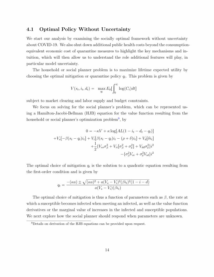
4.1 Optimal Policy Without Uncertainty

We start our analysis by examining the socially optimal framework without uncertainty

about COVID-19. We also shut down additional public health costs beyond the consumption-

equivalent economic cost of quarantine measures to highlight the key mechanisms and in-

tuition, which will then allow us to understand the role additional features will play, in

particular model uncertainty.

The household or social planner problem is to maximize lifetime expected utility by

choosing the optimal mitigation or quarantine policy qt. This problem is given by

V pst, it, dtq “ maxqt

E0r

ż 8

0

logpCtqdts

subject to market clearing and labor supply and budget constraints.

We focus on solving for the social planner’s problem, which can be represented us-

ing a Hamilton-Jacobi-Bellman (HJB) equation for the value function resulting from the

household or social planner’s optimization problem9, by

0 “ ´κV ` κ logrALp1´ it ´ dt ´ qtqs

`Vsr´βpst ´ qtqits ` Virβpst ´ qtqit ´ pρ` δqits ` Vdrδits

`1

2tVssσ

2β ` Viirσ

2β ` σ

2δ s ` Vddσ

2δui

2

´tσ2βVsi ` σ

2δVidui

2

The optimal choice of mitigation qt is the solution to a quadratic equation resulting from

the first-order condition and is given by

qt “´pκaq ˘

a

pκaq2 ` apVs ´ Viq2pβitq2p1´ i´ dq

apVs ´ Viqpβitq

The optimal choice of mitigation is thus a function of parameters such as β, the rate at

which a susceptible becomes infected when meeting an infected, as well as the value function

derivatives or the marginal value of increases in the infected and susceptible populations.

We next explore how the social planner should respond when parameters are unknown.

9Details on derivation of the HJB equations can be provided upon request.

14

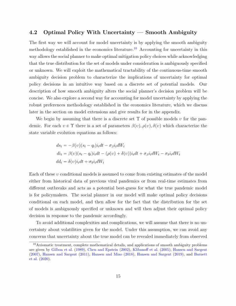
4.2 Optimal Policy With Uncertainty — Smooth Ambiguity

The first way we will account for model uncertainty is by applying the smooth ambiguity

methodology established in the economics literature.10 Accounting for uncertainty in this

way allows the social planner to make optimal mitigation policy choices while acknowledging

that the true distribution for the set of models under consideration is ambiguously specified

or unknown. We will exploit the mathematical tractability of the continuous-time smooth

ambiguity decision problem to characterize the implications of uncertainty for optimal

policy decisions in an intuitive way based on a discrete set of potential models. Our

description of how smooth ambiguity alters the social planner’s decision problem will be

concise. We also explore a second way for accounting for model uncertainty by applying the

robust preferences methodology established in the economics literature, which we discuss

later in the section on model extensions and give results for in the appendix.

We begin by assuming that there is a discrete set Υ of possible models υ for the pan-

demic. For each υ P Υ there is a set of parameters βpυq, ρpυq, δpυq which characterize the

state variable evolution equations as follows:

dst “ ´βpυqpst ´ qtqitdt´ σβitdWt

dit “ βpυqpst ´ qtqitdt´ pρpυq ` δpυqqitdt` σβitdWt ´ σδitdWt

ddt “ δpυqitdt` σδitdWt

Each of these υ conditional models is assumed to come from existing estimates of the model

either from historical data of previous viral pandemics or from real-time estimates from

different outbreaks and acts as a potential best-guess for what the true pandemic model

is for policymakers. The social planner in our model will make optimal policy decisions

conditional on each model, and then allow for the fact that the distribution for the set

of models is ambiguously specified or unknown and will then adjust their optimal policy

decision in response to the pandemic accordingly.

To avoid additional complexities and complications, we will assume that there is no un-

certainty about volatilities given for the model. Under this assumption, we can avoid any

concerns that uncertainty about the true model can be revealed immediately from observed

10Axiomatic treatment, complete mathematical details, and applications of smooth ambiguity problemsare given by Gilboa et al. (1989), Chen and Epstein (2002), Klibanoff et al. (2005), Hansen and Sargent(2007), Hansen and Sargent (2011), Hansen and Miao (2018), Hansen and Sargent (2019), and Barnettet al. (2020).

15

outcomes. Though the analysis can be extended to such settings under proper conditions,

this assumption allows us to carry out a revealing analysis of the impact of uncertainty un-

der the smooth-ambiguity based decision theoretic framework in a straightforward manner.

For each υ conditional model the social planner solves a conditional problem maximizing

lifetime expected utility by choosing the optimal mitigation or quarantine policy qtpυq

conditional on the given υ model. This conditional problem is given by

V pst, it, dt; υq “ maxqtpυq

E0r

ż 8

0

logpCtpυqqdt|υs

subject to market clearing and labor supply and budget constraints.

We can represent the solution for the value function V pυq using a Hamilton-Jacobi-

Bellman (HJB) equation resulting from the household or social planner optimization prob-

lem, which is given by

0 “ ´κV pυq ` κ logrALp1´ it ´ dt ´ qtpυqqs

`Vspυqr´βpst ´ qtpυqqits ` Virβpυqpst ´ qtpυqqit ´ pρpυq ` δpυqqits ` Vdpυqrδpυqits

`1

2tVsspυqσ

2β ` Viipυqrσ

2β ` σ

2δ s ` Vddpυqσ

2δui

2

´tσ2βVsipυq ` σ

2δVidpυqui

2

The optimal choice of mitigation qtpυq is the solution to a quadratic equation resulting

from the first-order condition and is given by

qtpυq “´pκaq ˘

a

pκaq2 ` apVspυq ´ Vipυqq2pβpυqitq2p1´ i´ dq

apVspυq ´ Vipυqqpβpυqitq

The optimal choice of mitigation is now a function of the conditional model parame-

ters βpυq, and the conditional marginal values of changes to the susceptible and infected

populations, represented by Vspυq, Vipυq.

To incorporate uncertainty, we will now apply the decision theoretic framework devel-

oped in Hansen and Sargent (2011) and Hansen and Miao (2018). We first specify a prior

distribution to the set of models υ P Υ, by assigning a probability weight πpυq to each

model υ. Note that for these weights to be well defined as probability weights they must

satisfy the following conditions:

πpυq ě 0, @υ

16

ÿ

υPΥ

πpυq “ 1.

Like the alternative models in our set, the prior probability weights are assumed to come

from historical data or real-time observational inference.

We then allow for uncertainty aversion by using a penalization framework based on

conditional relative entropy. This framework allows the planner to consider alternative

distributions or sets of weights πpυq across the set of conditional models in a way that

is statistically reasonable by restricting the set of alternative models considered by the

social planner to those that are difficult to distinguish from the prior model distribution

using statistical methods and past data.11 The parameter θa is chosen to determine the

magnitude of this penalization. Relative entropy is defined as the expected value of the

log-likelihood ratio between two models or the expected value of the log of the Radon-

Nikodym derivative of the perturbed model with respect to approximating one. The value

of relative entropy is weakly positive, and zero only when the models are the same.12

This new, second-stage problem for the planner is a minimization problem, where the

minimization is made over possible distorted probability weights πpυq which are constrained

by θa based on the solutions to the υ conditional value function solutions found previously.

This allows the planner to determine the relevant worst-case model for given states of

the world to help inform their optimal policy decisions. Though optimal decisions will

be determined by considering alternative worst-case models, this setting should not be

interpreted as a distorted beliefs model. The worst-case model is used as a device to

produce solutions that are robust to alternative models. The second-stage minimization

problem is given by the solution to the following problem

Vt “ minπpυq

ÿ

˜πpυqpV pυq ` θarlogpπpυqq ´ logpπpυqqsq

11To give a concrete example in the context of COVID-19, it may be relatively easy to observe thenumber of people who died from the pandemic but difficult to observe the number of people who wereinfected. On the basis of this data, it is difficult to tell whether the disease has a very high spread rate(R0) and a low death rate (CFR), or a low spread rate and a very high death rate, yet the optimal responseis likely to be very different under these scenarios.

12See Hansen and Sargent (2011) for details about relative entropy in this setting. Using relative entropymeans we are only considering relatively small distortions from the baseline model, but even small distor-tions can have significant impacts on optimal policy. In particular, we apply relative entropy penalizationdirectly to the set of conditional value functions. We could instead apply relative entropy penalization tothe stochastic increments of the model, which would require that we scale relative entropy linearly by dtand solve a single, non-linearly adjusted HJB equation, but we find the current framework tractable andappealing for comparison with the outside the model sensitivity analysis we will conduct later on.

17

subject toÿ

πpυq “ÿ

πpυq “ 1

Taking the first order condition for this problem, and imposing the constraintř

πpυq “

1, we can solve for the optimally distorted probability weights, which are given by

πpυq “πpυq expp´1

θV pυqq

ř

πpυq expp´ 1θaV pυqq

As the πpυq in the model are optimally determined and state dependent, the magnitude

of the ambiguity considered by the social planner when making optimal policy decisions

will depend on the current state of the pandemic and evolve dynamically. Plugging the

optimally distorted probability weights back into the optimization problem provides us

with the optimized value function under smooth ambiguity

Vt “ ´θ logrÿ

πpυq expp´1

θaV pυqqs

For both the distorted probability weights and the optimized value function under un-

certainty, we see that smooth ambiguity plays the role of imposing an exponential tilting

towards those υ conditional models that lead to the most negative lifetime expected utility

implications. A smaller value of θa enhances the magnitude of the concern about ambiguity,

and the prior probability weights play an important role for anchoring the outcomes to a

baseline expectation of the true model. In order to determine the ambiguity robust policy

for the social planner, we weight the υ conditional optimal mitigation policies qtpυq using

the distorted probability weights to get

qt “ÿ

υ

πpυqqtpυq

The exponential tilting of the distorted probability weights carries through to our deter-

mination of the optimal mitigation strategy. The magnitude with which we weight each

υ conditional model informs us how to weight the υ conditional mitigation policy as well.

Finally, this same reweighting by the distorted probability weights provides us with the

distorted parameters which the social planner uses to make optimal policy decisions in this

setting, which are given by

βt “ÿ

υ

πpυqβpυq

18

δt “ÿ

υ

πpυqδpυq

As the planner tilts their value function and probability weights towards certain models,

this leads to the implied distorted model parameters which are informed by worst-case

outcomes which the planner uses as a lens to view and respond in a robustly optimal way

in the face of uncertainty.

5 Numerical Results

We will now provide numerical results from simulations based on the theoretical solutions

provided above. We will first show results based on the set of model solutions solved

assuming no uncertainty in an “outside the model” sensitivity analysis. These results

show the dispersion in possible model outcomes even when the planner does not account

for uncertainty and indicate the importance of accounting for uncertainty by the social

planner. We will then show the role of “inside the model” uncertainty using three different

scenarios: (i) when the social planner has underestimated the pandemic; (ii) when the social

planner has correctly guessed the true model for the pandemic; and (iii) when the social

planner has overestimated the pandemic. For each scenario we will show the outcomes

assuming the planner knows the true model, the outcomes based on the assumed prior but

not accounting for model uncertainty, and the outcomes based on the assumed prior but

accounting for model uncertainty. We focus our “inside the model” uncertainty numerical

results on the smooth ambiguity solution for two reasons. First, while the robustness setting

has distinct and important features to consider, the numerical results (which we provide

in the appendix) turn out to be quite similar to the smooth ambiguity results. Second,

the smooth ambiguity setting allows us to explore how the social planner weighs the set of

possible models in making optimal decisions, a particularly valuable and revealing result

that will provide intuition for the observed results in our numerical analysis.

5.1 Calibration

There are a number of economic and pandemic related parameters that we choose values for

that we discuss now. For the economic side of the model, we assume a working population

of 164 million, consistent with the total US labor supply, and that per worker weekly output

is given by $2, 345 so that output in the non-pandemic version of the model (AˆL) matches

19

recent, pre-pandemic data on weekly US GDP of $384 billion dollars. We choose an annual

discount rate of 2%, and so the subjective discount rate κ, the weekly counterpart to this

value, is given by κ “ 0.000384. For the baseline analysis, we assume a convex quarantine

cost structure where a “ 1.25 and b “ 2.

For the pandemic model parameters, we use values from various studies (including

Korolev (2020), Atkeson (2020b), Atkeson (2020a), Wang et al. (2020), and estimates

fromm the European Centre for Disease Prevention and Control) to set the expected time

infected γ, the case fatality rate CFR, and the birth rate R0, which allows us to pin down

the infection rate β, the death rate δ, and the recovery rate ρ. The value of γ is held fixed

at γ “ 718

. The set of underlying models used in our analysis use values of CFR in the set

t0.005, 0.02, 0.035u and values of R0 in the set t2.0, 3.5, 5.0u. These values are well within

the range of values across these different studies. For the volatilities σβ and σδ, we use data

from the Center for Systems Science and Engineering in the Whiting School of Engineering

at Johns Hopkins University13 to calculate empirical counterparts for these values.

Finally, we must also specify values for the uncertainty parameters in our model, θa

for smooth ambiguity and θm for robust preferences. Our values of θm and θm impose

significant amounts of uncertainty aversion to demonstrate the potential magnitude of

uncertainty impacts. The values we use are θa “ 0.00004 and θm “ 0.0067. These values

can be difficult to interpret on their own, and are best interpreted by way of the conditional

relative entropy values implied by these parameter choices and statistical discrimination

bounds related to these conditional relative entropy values. In the model extensions section

we discuss methods we will use to help discipline and calibrate our uncertainty parameter

choices going forward based on these two criteria and from anecdotal evidence on model

spreads implied by the recent estimates of COVID-19 parameter values.

5.2 Model Simulations

5.3 Outside the Model Uncertainty Through Sensitivity Analysis

We first provide simulated outcomes of the model based on different pandemic models

without the planner accounting for uncertainty in their optimal decision. This corresponds

to what is typically termed as a sensitivity analysis. It serves to illustrate the wide range

of optimal responses and outcomes that depend on the underlying model parameters. This

by itself is not a rigorous robust optimal control approach to model uncertainty. What

13This data is available through the CSSE GitHub repo.

20

the robust optimal control frameworks will provide are frameworks for the policymaker

to optimally choose a single policy, simultaneously taking into account the variation in

optimal responses across different pandemic models.

Figure 4 shows the spread of outcomes for st, it, rt, dt, and qt across the different model

cases. This is what is sometimes called “outside the model” uncertainty, or uncertainty

in outcomes without accounting for how the decision makers choices are impacted by the

uncertainty. The spreads are across all model outcomes for R0 P t2, 3.5, 5u and CFR P

t0.005, 0.02, 0.035u. Figure 4 indicates very different outcomes for s, i, r, d, and q, depending

on model cases. The fact that outcomes change so drastically is suggestive that uncertainty

about parameters may have important effects on optimal policy. Observe that across the

models, the fraction of the dead population after 104 weeks varies by an order of magnitude,

from less than 0.5% to nearly 2.5%. More strikingly, these are the death rates obtained by

a policy maker that knows the true parameters and is reacting optimally, and in that sense

provides a best-case outcome under each scenario.

21

Figure 4: Outside the Model Uncertainty

Notes: These figures show the range of possible outcomes and policy responses across nine potential models

of the pandemic that vary by their R0 and CFR. From left to right, top to bottom, we show the fraction

of the population that is susceptible, the fraction of the population that is infected, the fraction of the

population that has had the disease and recovered, the fraction of the population that has died, and the

fraction of the population under quarantine. We show the maximum and minimum for these variables across

each model. 22

Figure 5: Outside the Model Uncertainty

Notes: These figures show the range of possible outcomes and policy responses across models of the pandemic

that vary by their R0 and CFR by the optimal quarantine policy. From left to right, top to bottom, we

show the fraction that is susceptible, the fraction that is infected, the fraction that has had the disease and

recovered, the fraction that has died, and the fraction under quarantine. The green shaded region shows

spread of the simulated outcomes without any mitigation and the red shaded region shows the spread of the

simulated outcomes with optimal mitigation. We show the maximum and minimum across each model.

23

Figure 5 augments our outside the model uncertainty comparison by adding to Fig-

ure 4 the spread of st, it, rt and dt across the different model cases if qt “ 0. Again

these plots use the model specifications with combinations of R0 P t2, 3.5, 5u and CFR

P t0.005, 0.02, 0.035u. This figure not only demonstrates how critical mitigation and quar-

antine measures are in controlling a pandemic, but how much wider the spread can be if

the planner does not take optimal policy action. The magnitude of pandemic impacts vary

drastically depending on which model is the true underlying pandemic model, with some

cases featuring much more rapid realization of the pandemic impacts and the number of

dead and infected dramatically higher. Observe that across the models without quarantine,

the fraction of the dead population after 104 weeks varies even more, from less than 0.5%

to almost 3.5%. Furthermore, of the three peaks for infections, based on the three different

R0 values, the worst reaches nearly 50%. These results further highlight the significant im-

portance of quarantine measures and how severe a pandemic outbreak can be if the social

planner making optimal policy has to respond without knowing the true model.

5.4 Inside the Model Uncertainty Through Smooth Ambiguity

Conditional on each model, the social planner’s problem trades off short-term mitigation

costs with long-term pandemic-related death and illness costs, and the need for a longer-

lasting quarantine. More severe initial quarantine measures reduce the spread of the pan-

demic at the cost of current temporary reductions in the labor supply, and therefore produc-

tion and consumption. However, less severe quarantine measures lead to increased deaths,

which permanently reduce the labor supply, production, and consumption. As a result,

even a small reduction in the number of deaths has a significant economic benefit, even

without accounting for the first-order non-monetary losses from losing loved ones. Time

discounting plays an important role, however, because the costs associated with quarantine

are borne immediately, while longer-term costs are realized in the future. In consequence,

immediately stopping all infections and deaths is also suboptimal. In short, regardless of

the underlying model and uncertainty among them, the social planner faces a non-trivial

tradeoff in enacting pandemic mitigation policies, but how this tradeoff should be optimally

balanced varies substantially across models.

As we previously highlighted, the spread on estimates for R0 and CFR from numerous

studies is substantial, and so understanding how policymakers can optimally respond in

the face of such uncertainty is particularly relevant for this, or any other, economic and

24

public health crisis. The infection rate β and death rate δ are the parameters in our

model we will focus on for understanding uncertainty, given their explicit connection to the

CFR and R0 and the significant uncertainty that exists about these parameters. Once we

introduce uncertainty, the worst-case outcomes are amplified. In this setting, the worst-case

concerns are that infection and death rates are potentially higher and thus the permanent

effects could possibly be much worse. In response, the planner shifts more weight to the

possibility of experiencing larger permanent, long-term costs in terms of increased deaths

because of the pandemic. As a result, at a high level, the social planner making optimal

decisions under model uncertainty will tend to increases current, short-term costs from

strengthening quarantine measures in a dynamic way to address these concerns.

The starting point for this analysis is the policy maker’s prior over the models, πpυq,

where υ is one of the possible models under consideration. We consider three scenarios,

where, relative to the true parameters, the policy maker’s prior (i) underestimates the

pandemic (ii) correctly estimates the pandemic and (iii) overestimates the pandemic. We

find through our analysis important asymmetries in policy responses across these different

scenarios. Broadly, the effect of incorporating uncertainty in decision making has little

effect when models correctly or overestimate the severity of a pandemic, limiting excess

economic costs from quarantine measures. However, in a situation where the severity of

the pandemic is initially underestimated and the disease is allowed to spread, incorporating

uncertainty moves policy significantly towards what the optimal policy response would be

had the social planner known the true underlying model.

We discuss these effects in detail, which are presented in Figures 6-10. In each figure,

we show the state variables and optimal policy responses in three series. We show (i) the

prior model response, which is the optimal response based on the policymaker’s assumed

prior distribution of probability weights across all models in consideration given the current

state of the world, representing what one might consider to be a “naive” approach to model

uncertainty where the policymaker acknowledges different potential models and adopts

a fixed distribution; (ii) is the true optimal response had the policy maker known the

true model; (iii) is the uncertainty adjusted response, where the policymaker optimally

weighs each model to arrive at her decision that is designed to be robust to possible model

uncertainty.

25

Figure 6: Scenario 1: Underestimating the Pandemic

Notes: These figures show (i) the prior model response (red), the true optimal response (black), and the

uncertainty-adjusted response (blue) in the case where the policy maker initially underestimates the severity

of the pandemic. From left to right, top to bottom, these figures are (1) the fraction of the population

that is susceptible to the disease, (2) the fraction of the population that is infected, (3) the fraction of the

population that has had the disease and recovered, (4) the fraction of the population that has died, and (5)

the fraction of the population in quarantine. 26

Figure 7: Scenario 1: Underestimating the Pandemic

Notes: These figures show (i) the prior model (red), the true model (black), and the uncertainty-adjusted

model (blue) parameter value in the case where the policy maker initially underestimates the severity of

the pandemic. From left to right, top to bottom, these figures are (1) the distorted probability weights πt,

(2) the infection rate βt, (3) the recovery rate ρt, and (4) the death rate δt. For the distorted probability

weights, the blue lines are for models with R0 “ 2.0, the red lines are for models with R0 “ 3.5, the yellow

lines are for models with R0 “ 5.0, the dashed-dotted lines are for models with CFR“ 0.005, the dashed

lines are for models with CFR“ 0.020, and the solid lines are for models with CFR“ 0.035.

27

Figure 8: Scenario 2: Correctly Estimating the Pandemic

Notes: These figures show (i) the prior model response (red), the true optimal response (black), and the

uncertainty-adjusted response (blue) in the case where the policy maker initially correctly estimates the

severity of the pandemic. From left to right, top to bottom, these figures are (1) the fraction of the population

that is susceptible to the disease, (2) the fraction of the population that is infected, (3) the fraction of the

population that has had the disease and recovered, (4) the fraction of the population that has died, and (5)

the fraction of the population in quarantine. 28

Figure 9: Scenario 2: Correctly Estimating the Pandemic

Notes: These figures show (i) the prior model (red), the true model (black), and the uncertainty-adjusted

model (blue) parameter value in the case where the policy maker initially correctly estimates the severity of

the pandemic. From left to right, top to bottom, these figures are (1) the distorted probability weights πt,

(2) the infection rate βt, (3) the recovery rate ρt, and (4) the death rate δt. For the distorted probability

weights, the blue lines are for models with R0 “ 2.0, the red lines are for models with R0 “ 3.5, the yellow

lines are for models with R0 “ 5.0, the dashed-dotted lines are for models with CFR“ 0.005, the dashed

lines are for models with CFR“ 0.020, and the solid lines are for models with CFR“ 0.035.

29

Figure 10: Scenario 3: Overestimating the Pandemic

Notes: These figures show (i) the prior model response (red), the true optimal response (black), and the

uncertainty-adjusted response (blue) in the case where the policy maker initially overestimates the severity

of the pandemic. From left to right, top to bottom, these figures are (1) the fraction of the population

that is susceptible to the disease, (2) the fraction of the population that is infected, (3) the fraction of the

population that has had the disease and recovered, (4) the fraction of the population that has died, and (5)

the fraction of the population in quarantine. 30

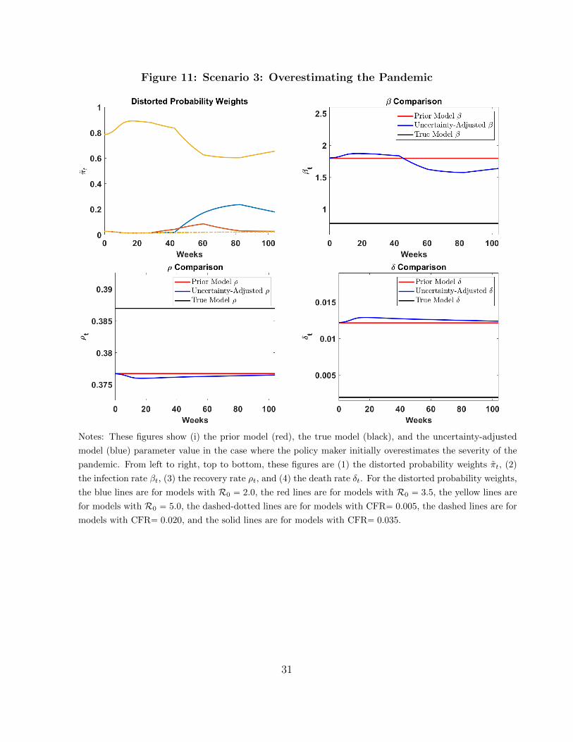
Figure 11: Scenario 3: Overestimating the Pandemic

Notes: These figures show (i) the prior model (red), the true model (black), and the uncertainty-adjusted

model (blue) parameter value in the case where the policy maker initially overestimates the severity of the

pandemic. From left to right, top to bottom, these figures are (1) the distorted probability weights πt, (2)

the infection rate βt, (3) the recovery rate ρt, and (4) the death rate δt. For the distorted probability weights,

the blue lines are for models with R0 “ 2.0, the red lines are for models with R0 “ 3.5, the yellow lines are

for models with R0 “ 5.0, the dashed-dotted lines are for models with CFR“ 0.005, the dashed lines are for

models with CFR“ 0.020, and the solid lines are for models with CFR“ 0.035.

31

The first case we consider is a case in which models underestimate the severity of the

new disease. Here the planner assumes the pandemic has a lower R0 and CFR than is true.

The prior distribution gives the model with R0 “ 2 and CFR“ 0.005 a weight of 7{9 and

the remaining weight equally distributed across the other eight models. The true model

parameters are given by R0 “ 5 and CFR“ 0.035. This case is shown in Figure 6. In this

case, the prior model optimal response leads to much lower mitigation efforts relative to the

true optimal response. This results in a sharp peak in infections and a much higher death

rate relative to the optimal response. The uncertainty adjusted response brings mitigation

levels very close to the true optimal, with a corresponding lower infection and death rate.

Figure 7 highlights the underlying mechanisms driving this result. The top left plot

shows the distorted probability weights that the planner uses when allowing for uncertainty.

Their initial values are driven by the assumed prior, which places a majority of the weight

on a low CFR, low R0 model represented by the dotted-dashed blue line and the remaining

weight equally split across all other models. As the pandemic evolves and infections and

deaths begin to occur, the planner allowing for uncertainty immediately shifts a significant

probability weight to the solid yellow line which represents the model with the highest CFR

and R0 values. This significantly increases the amount of quarantine done and diminishes

the impacts of the pandemic. As a result, the pandemic evolves at a much slower rate,

leading the planner to shift weight first to the high CFR and middle R0 value, then to the

high CFR and low R0 value, and finally back towards the model with the highest prior

weight. This occurs because the planner is not assumed to be learning, but rather reacting

to the observed current state of the pandemic. As a result of this significant uncertainty

reaction and strong uncertainty response early on, the pandemic plays out in a way that

is nearly as severe as what seemed possible at first, and thus the penalization attached

to uncertainty causes the planner to shift their view of what are statistically reasonable

worst-case models to consider. A high CFR is persistently relevant for the planner, but

because the planner is reacting based on concerns about uncertainty and not learning as in

a Bayesian setting, they then begin to revert back to the prior model their decision problem

is anchored to.

Intuitively, the penalization costs of allowing for a severe worst-case model are out-

weighed by the possible gains of making a policy choice that is robust to potentially signif-

icant uncertainty. As the pandemic winds down and the effects are limited by the strong

early response, the possibility for such large deviations from the assumed prior are less

likely and so the planner reduces their uncertainty penalization by considering less severe

32

worst-case models. The dynamics of the distorted probability weights lead to the remaining

outcomes we see in Figure 7. The black and red lines show that the planner initially un-

derestimates the pandemic by assuming a lower β and δ and a higher ρ (the red horizontal

lines) than is true (the black horizontal lines). As the pandemic worsens, the uncertain

planner shifts their distorted parameters β, δ and ρ (the blue lines) away from the prior

towards the true values and then winds those values back down towards the prior as the

pandemic resolves in a better than first anticipated way.

In the next two cases we consider, incorporating uncertainty has much more muted

effects on the optimal response and outcomes. The second case we consider is a case in

which models correctly estimate the severity of the new disease. The planner’s assumed

prior distribution gives each model of R0 and CFR an equal weight of 1{9 which is the

same R0 and CFR as the true model. This case is shown in Figure 8. In this scenario,

incorporating uncertainty into the response has a much more moderate effect. Mitigation

efforts, though similar under both the optimal and uncertainty adjusted response, are

slightly higher early on and persistently higher over time. Infection and death rates are

also similar, though they peak higher under quarantine policy made without consideration

for model uncertainty and result in an increase in deaths as well.

Figure 9 demonstrates the underlying mechanisms driving this mode muted response.

As in the first scenario, the distorted probability weights start near the assumed prior that

gives equal weight to all the models. As before, once the infections and deaths increase the

planner then shifts a significant probability weight first to the highest CFR and R0 model,

and the resulting decrease in infections and deaths resulting from the strong quarantine

response early on leads to a shift to the high CFR and middle R0 model and finally to

the high CFR and low R0 model. The probability weights then begin to converge back

to the prior, but in this case that means reducing the weight on the high CFR model and

increasing weights on all the other models. This response, while similar in the fact that

the high CFR models play a key role leading to a strong and fast quarantine response, the

differences are far more muted because the pandemic never has a chance to reach the levels

of infections and deaths that would lead to drastic uncertainty responses. The planner

overreacts by overshooting what the worst case β, ρ, and δ might be at first, but because

the true model matches their prior the value of considering more severe worst-case models

for longer at the cost of larger uncertainty penalization is never realized.

The third case we consider is a case in which models over estimate the severity of the

new disease. The planner here assumes the pandemic has a higher R0 and CFR than is

33

true and the assumed prior distribution gives the model with R0 “ 5 and CFR“ 0.035

a weight of 7{9 and the remaining weight equally distributed across the remaining eight

models. The true model parameters, however, are given by R0 “ 2 and CFR“ 0.005. This

case is shown in Figure 10. In this case, again incorporating uncertainty into the response

has very little effect, and policy and outcomes are nearly identical under the prior model

and uncertainty adjusted responses. Both the prior model and the uncertainty adjusted

responses lead to overly high mitigation efforts, and low infection and death rates to the

optimum given economic damages from the mitigation policy. This result demonstrates the

key asymmetry: optimal policy while accounting for uncertainty is significantly closer to

the optimal policy when made knowing the true model when underestimating the model,

but is no worse than the no uncertainty policy choice in terms of excess quarantine measures

and therefore excess economic losses when overestimating the model.

For this scenario, Figure 11 highlights the key model tradeoffs leading to the planner

behaving essentially as if he is not uncertain. Because initial distorted probability weights

near the assumed prior of a high CFR and high R0 illicit a higher than optimal quarantine

response, the pandemic never reaches states where there is much value to considering more

severe worst-case pandemic models at the cost of increased penalization. In fact, there is

almost no additional overreaction in this case because infections and deaths increased much

slower than the prior model would have suggested. As a result the distorted probability

weights stay much more stable and closer to the prior, and only slowly begin to disperse

more weight to the models with high CFR and middle and low R0 values. This causes

the planner to maintain a view on the distorted or potential worst case β, ρ, and δ values

that also remain very close to the prior values assumed for these parameters. Because

of the concern for possible uncertainty, the planner never is able to underreact, which

would actually reduce quarantine levels and increase output by allowing more individuals

to work. However, uncertainty has essentially no worse economic or welfare implications in

this scenario than just assuming the prior model but without aversion to ambiguity.

In future work, we plan to quantify these outcomes in terms of welfare and economic

impacts. These valuations will help demonstrate that the effects of model uncertainty, even

under relatively modest aversion to uncertainty, can be economically significant and critical

to account for in optimal policy decisions related to COVID-19 and other pandemics.

34

6 Model Extensions

Infection Dependent Death Rate

Following Eichenbaum, Rebelo, and Trabandt (2020) and others, we can account for con-

cerns that the healthcare system could be overwhelmed by the number of infected individ-

uals, leading to an increased CFR. To model this, we can specify, as others have done, that

the death rate is given by

δt “ δ ` δ`i2t

This framework will not lead to any changes to the functional form for the optimal

quarantine choice, but can have significant implications on the value function and will alter

the numerical value of the optimal policy choice. Using our framework for understanding

uncertainty, we can account for uncertainty about this more generalized specification for

the death rate δt and determine how this state dependent death rate influences economic

outcomes and decisions about quarantine, with and without uncertainty, across the different

scenarios that we consider. By taking multiple estimates of δ` based on various estimates

or measurements from different COVID-19 outbreaks, we can augment our set of pandemic

models and conduct a similar analysis to what we have done here to account for this

potentially important feature.

Productivity Costs of Mitigation and Uncertainty

An important extension to consider is the possibility of additional costs of quarantine

measures on output, beyond the consumption-equivalent costs that result from reduced

labor. In addition, a potential consequence of mitigation efforts is that it could lead to

reduction in productivity. In particular, Barrot, Grassi, and Sauvagnat (2020) note that

social distancing measures could lead to a reduction in GDP growth. We model this

formally by extending our expression of productivity to be

A “ A exppztq

dzt “ µzdt´1

2σ2zdt` σzdWt

This extends productivity to follow standard geometric Brownian motion growth as is

commonly used throughout economics and financial modeling. However, we add to this a

35

term to account for reduced growth resulting from social distancing quarantine measures,

which we will calibrate to fit the estimates provided by Barrot, Grassi, and Sauvagnat

(2020). This additional term augments the process for z to now be

A “ A exppztq

dzt “ µzdt´ aqbtdt´

1

2σ2zdt` σzdWt

The cost provides an additional impact from quarantine reflected in not only level im-

pacts but also growth implications for quarantine measures. In addition, as there exists

substantial uncertainty about the long-term economic consequences of “shutting down the

economy” in this manner, we can allow for this additional channel of model uncertainty

as we have done with the pandemic model, allowing for alternative values of a, b to be

specified and part of our υ conditional models so that dzt is given b

A “ A exppztq

dzt “ µzdt´ apυqqbpυqt dt´

1

2σ2zdt` σzdWt

This additional additional channel of uncertainty will interact with our existing uncertain-

ties and will potentially have meaningful implications for the social planner’s optimal policy

response to the COVID-19 pandemic.

Uncertainty Through Robustness

Though our analysis mainly used the smooth ambiguity framework, where the social plan-

ner optimally chose probability weights to place on competing parameterizations of the

model, an alternate approach to the problem is through applying the robust preferences

methodology established in the economics literature14. Accounting for uncertainty in this

way allows the social planner to make optimal mitigation policy choices while acknowl-

edging that a given baseline model may be misspecified. As with smooth ambiguity, the

mathematical tractability of the robust preferences decision problem allows us to charac-

terize the implications of uncertainty for optimal policy decisions with clear intuition. We

14Detailed explanations of robust preference problems and axiomatic treatment of such formulations usingpenalization methods are given by Cagetti, Hansen, Sargent, and Williams (2002), Anderson, Hansen, andSargent (2003), Hansen, Sargent, Turmuhambetova, and Williams (2006), Maccheroni, Marinacci, andRustichini (2006), and Hansen and Sargent (2011).

36

briefly outline here how we incorporate robust preferences to account for model uncertainty,

and direct readers to the aforementioned references for complete mathematical details.

We define the approximating or baseline model using the evolution equations of the

state variables as previously given:

dst “ ´βpst ´ qtqitdt´ σβitdWt

dit “ βpst ´ qtqitdt´ pρ` δqitdt` σβitdWt ´ σδitdWt

ddt “ δitdt` σδitdWt

As was the case in the smooth ambiguity setting, we assume the baseline model is the result

of historical data or previous information about coronavirus pandemics and acts as a best-

guess at what the true COVID-19 pandemic model is for policymakers. However, we allow

the social planner in our model to consider the likelihood that this model is misspecified, or

that there are possibly other models which are the true model for the COVID-19 pandemic.

Possible alternative models are represented by a drift distortion that is added to the

approximating model by changing the Brownian motion Wt to Wt`şt

0hsds where hs and Wt

are processes adapted to the filtration generated by the Brownian motion Wt. Therefore,

alternative models under consideration by the social planner are of the form

dst “ r´βpst ´ qtqit ´ htσβitsdt´ σβitdWt

dit “ rβpst ´ qtqit ´ pρ` δqit ` htσβit ´ htσδitsdt` σβitdWt ´ σδitdWt

ddt “ rδit ` htσδitsdt` σδitdWt

In this form, the alternative models are disguised by the Brownian motion and so are

hard to detect statistically using past data. In addition, the alternative models are given

without direct parametric form, which allows for a larger class of alternative models under

consideration by the planner.

We can interpret the drift perturbations for misspecification directly as parameter mis-

specifications and altered model parameters of the form

dst “ r´βpst ´ qtqitsdt´ σβpst ´ qtqitdWt

dit “ rβpst ´ qtqit ´ pρ` δqitsdt` σβpst ´ qtqitdWt ´ σδitdWt

ddt “ rδitsdt` σδitdWt

37

where β “ β `htσβps´qq

and δ “ δ ` htσδ. The ht in the model will be optimally determined

and state dependent, and so the magnitude of the parameter misspecification considered by

the social planner when making optimal policy decisions will depend on the current state

of the pandemic and evolve dynamically.

For the uncertainty analysis to be reasonable, we will restrict the set of alternative

models considered by the social planner to those that are difficult to distinguish from the

baseline model using statistical methods and past data. A penalization term based on the

conditional relative entropy measure of model distance is used to accomplish this. The

parameter θm is chosen to determine the magnitude of this penalization. We have defined

relative entropy previously, and note that Hansen, Sargent, Turmuhambetova, and Williams

(2006) provides complete details about relative entropy use in a robust preferences setting.

Again, relative entropy means we are only considering relatively small, though potentially

significant, distortions from the baseline model.

The time derivative of relative entropy or contribution of the current worst-case model

htdt to relative entropy is given by 12|ht|

2. This term is added to the flow utility or pref-

erences of the household to account for model uncertainty. As was the case in the smooth

ambiguity setting, optimal decisions will be determined by considering alternative worst-

case models as a device to generate optimal policies that are robust to alternative models,

and not as some type of distorted beliefs setting. The household maximization problem is

replaced with a max-min set-up, where the minimization is made over possible model dis-

tortions h˚t which are constrained by θm. This allows the planner to determine the relevant

worst-case model for given states of the world to help inform their optimal policy decisions.

While we have incorporated additional structure and complexity to the model to account

for model uncertainty, the resulting household or social planner problem remains tractable

and similar to the previous, no uncertainty problem, and is given by

V pst, it, dtq “ maxqt

minht

E0r

ż 8

0

tlogpCtq `θ

2|ht|

2udts

subject to market clearing and labor supply constraints.

As before, the social planner’s solution is still characterized by a recursive Markov equi-

librium for which an equilibrium solution is defined as before. The HJB equation resulting

from this modified household or social planner optimization problem which characterizes

38

the socially optimal solution is now given by

0 “ ´κV ` κ logrALp1´ it ´ dt ´ qtqs `θ

2|ht|

2

`Vsr´βpst ´ qtqit ´ htσβits ` Virβpst ´ qtqit ´ pρ` δqit ` htσβit ´ htσδits

`Vdrδit ` htσδits `1

2tVssσ

2β ` Viirσ

2β ` σ

2δ s ` Vddσ

2δui

2t

´tσ2βVsi ` σ

2δVidui

2t

The first-order conditions for the optimal model distortions give us

|ht|2“

1

θ2rpVi ´ Vsq

2pσβitq

2` pVd ´ Viq

2pσδitq

2s

Plugging back in to the HJB equation, we are left with the following problem

0 “ ´κV ` κ logrALp1´ it ´ dt ´ qtqs

´1

2θrpVi ´ Vsq

2pσβitq

2` pVd ´ Viq

2pσδitq

2s

`Vsr´βpst ´ qtqits ` Virβpst ´ qtqit ´ pρ` δqits ` Vdrδits

`1

2tVssσ

2β ` Viirσ

2β ` σ

2δ s ` Vddσ

2δui

2t

´tσ2βVsi ` σ

2δVidui

2t

The optimal choice of mitigation qt is the solution to a quadratic equation resulting from

the first-order condition and is given by

qt “´pκALaq ˘

a

pκALaq2 ` ALapVs ´ Viq2pβitq2rALp1´ i´ dq ´ γ1i´ γ2ρis

ALapVs ´ Viqpβitq

Key differences to the social planner problem and HJB equation show up through the

adjustments to the flow utility as a result of the penalization term accounting for model

uncertainty concerns. The optimal mitigation policy takes the same functional form as

before. The implications of model uncertainty for optimal mitigation policy and social

welfare in the face of a pandemic are not only the direct adjustments to the key equations

of interest, but also how these adjustments feed through the model solution and alter the

value function V and the marginal values of changes to the susceptible, infected, and dead

populations, represented by Vs, Vi, Vd. Though we do not report results from this approach,

the high-level findings mirror closely those under the smooth ambiguity approach.

39

6.1 Disciplining our analysis of model uncertainty

As we have introduced new parameters to our model, the parameters for model uncertainty

θa and θm, it is important to discipline them in a meaningful way. To do this for the

robustness case, we can calibrate θm based on bounds of statistical model discrimination

based on methods developed and extended by Chernoff (1952), Newman and Stuck (1979),

and Anderson, Hansen, and Sargent (2003). Furthermore, the spread on estimates from

the recent papers estimating the CFR and R0 will provide further anecdotal constraints.

Solving the model and determining the magnitude of relative entropy and model distortion

implied by the choice of θm, we can compare how these distortions compare to the parameter

values estimated in the literature and the implied statistical discrimination bounds to

determine reasonable values of θm. We can then compare these bounds and results to the

smooth ambiguity case to determine reasonable values of θa as well. While we currently

use values of θm and θm that impose significant amounts of uncertainty aversion without

calibrating them, we plan to use these methods going forward.

The method of statistical model discrimination we will use is for the robustness based

uncertainty measure is based on bounds derived by Chernoff (1952) for the error of statis-

tical detection between two models and Newman and Stuck (1979) who derived this bound

for a Markov counterpart. The bounds are based on a simplified, two-case model detection

problem where a decision maker tries statistically discriminate between the baseline model

and the worst-case model. The relevant bound comes from determining the probability

that the decision maker makes a type I or type II error in determining the true model

while choosing between the two possible models. We focus on an approximation of this

bound demonstrated by Anderson, Hansen, and Sargent (2000), Anderson, Hansen, and

Sargent (2003), and Hansen, Sargent, Turmuhambetova, and Williams (2006) that uses a

minimization of the implied local decay rate bound

εN ď “1

2expp´NΘ1

q

where Θ1 is given by

Θ1“ max

0ďrď1

1

2pr ´ 1qrhth

1t “

1

8hth

1t.

Here εN is the probability of making a type I or type II error in detecting the true model

and N is the data sample size. We use N “ 260 weeks, or 5 years for our sample size to

40

learn from. This approximate bound is still a conditional measure of model discrimination

that is state-dependent, and we will use this to discipline what is a reasonable value of θ,

along with comparisons of the distorted model parameters to estimates from other papers

studying COVID-19, for our analysis of model misspecification.

7 Concluding Remarks

This paper shows how to incorporate uncertainty in models of pandemics. Our main results

focus on the role of uncertainty aversion in a smooth ambiguity-based decision problem,

but we also show how a robust control approach would be implemented as well. With new

diseases, or diseases that have only had small outbreaks, there is often significant uncer-

tainty about key parameters which determine the overall costs of an epidemic. The results

highlight important asymmetries that may be present in many robust control problems. In-

corporating uncertainty into responses are particularly important when the assumed prior

model underestimates the severity of a new threat in terms of responding in a way that

is much closer to the optimal response when the true model is know. On the other hand,

though incorporating uncertainty does lead to an overreaction compared to traditional

approaches when the assumed prior matches the true model, the overreaction is fairly

moderate and the uncertainty-based response and traditional approach are nearly identical

when the assumed prior model overestimates the true values of a new threat.

Our analysis provides a framework under which uncertainty and model misspecification

can be incorporated into macroeconomic models of epidemics. Our work emphasizes the

that uncertainty can play a large role in determining the optimal policy response to a new

disease. Economists and epidemiologists, rather than using a range of parameters, can use

our framework to explicitly model uncertainty. Future work can focus on making these

models more tractable for policymakers, who often have to make decisions in real time.

41

References

Acemoglu, D., V. Chernozhukov, I. Werning, and M. Whinston (2020). A multi-risk sir model withoptimally targeted lockdown. Technical report, National Bureau of Economic Research.

Allcott, H., L. Boxell, J. Conway, M. Gentzkow, M. Thaler, and D. Y. Yang (2020). Polarization andpublic health: Partisan differences in social distancing during the coronavirus pandemic. NBER WorkingPaper (w26946).

Anderson, E., L. P. Hansen, and T. J. Sargent (2000). Robustness, Detection and the Price of Risk.Working Paper .

Anderson, E. W., L. P. Hansen, and T. J. Sargent (2003). A Quartet of Semigroups for Model Specification,Robustness, Prices of Risk, and Model Detection. Journal of the European Economic Association 1 (1),68–123.

Arrow, K. J. (1951). Alternative approaches to the theory of choice in risk-taking situations. Econometrica:Journal of the Econometric Society , 404–437.

Atkeson, A. (2020a). How deadly is covid-19? understanding the difficulties with estimation of its fatalityrate. Technical report, National Bureau of Economic Research.

Atkeson, A. (2020b). What will be the economic impact of covid-19 in the us? rough estimates of diseasescenarios. Technical report, National Bureau of Economic Research.

Avery, C., W. Bossert, A. Clark, G. Ellison, and S. F. Ellison (2020). Policy implications of models ofthe spread of coronavirus: Perspectives and opportunities for economists. Technical report, NationalBureau of Economic Research.

Baker, S. R., N. Bloom, and S. J. Davis (2016). Measuring economic policy uncertainty. The QuarterlyJournal of Economics 131 (4), 1593–1636.

Baker, S. R., N. Bloom, S. J. Davis, and S. J. Terry (2020). Covid-induced economic uncertainty. Technicalreport, National Bureau of Economic Research.

Baker, S. R., R. A. Farrokhnia, S. Meyer, M. Pagel, and C. Yannelis (2020a). How does household spendingrespond to an epidemic? consumption during the 2020 covid-19 pandemic. Technical report, NationalBureau of Economic Research.

Baker, S. R., R. A. Farrokhnia, S. Meyer, M. Pagel, and C. Yannelis (2020b). Income, liquidity, and theconsumption response to the 2020 economic stimulus payments. Technical report, National Bureau ofEconomic Research.

Baldauf, M., L. Garlappi, and C. Yannelis (2019). Does climate change affect real estate prices? only ifyou believe in it. Review of Financial Studies, Forthcoming .

Barnett, M., W. Brock, and L. P. Hansen (2019). Pricing Uncertainty Induced by Climate Change.University of Chicago Becker Friedman Institute for Economics Working Paper No. 2019-109. Availableat SSRN: https://ssrn.com/abstract=3440301 .

Barnett, M., W. Brock, and L. P. Hansen (2020). Pricing uncertainty induced by climate change. TheReview of Financial Studies 33 (3), 1024–1066.

42

Barrios, J. and Y. Hochberg (2020). Risk perception through the lens of politics in the time of the covid-19pandemic. Working Paper .

Barro, R. J., J. F. Ursua, and J. Weng (2020). The coronavirus and the great influenza pandemic: Lessonsfrom the “spanish flu” for the coronavirus’s potential effects on mortality and economic activity. Tech-nical report, National Bureau of Economic Research.

Barrot, J.-N., B. Grassi, and J. Sauvagnat (2020). Sectoral effects of social distancing. Working Paper .

Bloom, N. (2009). The impact of uncertainty shocks. Econometrica 77 (3), 623–685.

Burke, M., W. M. Davis, and N. S. Diffenbaugh (2018). Large Potential Reduction in Economic DamagesUnder UN Mitigation Targets. Nature 557 (7706), 549.

Cagetti, M., L. P. Hansen, T. Sargent, and N. Williams (2002). Robustness and pricing with uncertaingrowth. The Review of Financial Studies 15 (2), 363–404.

Chater, N. (2020). Facing up to the uncertainties of covid-19. Nature Human Behaviour , 1–1.

Chen, Z. and L. Epstein (2002). Ambiguity, risk, and asset returns in continuous time. Econometrica 70 (4),1403–1443.

Chernoff, H. (1952). A measure of asymptotic efficiency for tests of a hypothesis based on the sum ofobservations. The Annals of Mathematical Statistics, 493–507.

Coibion, O., Y. Gorodnichenko, and M. Weber (2020). Labor markets during the covid-19 crisis: Apreliminary view. Fama-Miller Working Paper .

Colacito, R., B. Hoffmann, and T. Phan (2018). Temperatures and growth: A panel analysis of the unitedstates. Journal of Money, Credit, and Banking 51 (2-3), 2019.

Coven, J. and A. Gupta (2020). Disparities in mobility responses to covid-19. Technical report.

Dell, M., B. F. Jones, and B. A. Olken (2012). Temperature Shocks and Economic Growth: Evidence fromthe Last Half Century. American Economic Journal: Macroeconomics 4 (3), 66–95.

Eichenbaum, M. S., S. Rebelo, and M. Trabandt (2020). The macroeconomics of epidemics. Technicalreport, National Bureau of Economic Research.

Gilboa, I., D. Schmeidler, et al. (1989). Maxmin expected utility with non-unique prior. Journal ofMathematical Economics 18 (2), 141–153.

Gormsen, N. J. and R. S. Koijen (2020). Coronavirus: Impact on stock prices and growth expectations.University of Chicago, Becker Friedman Institute for Economics Working Paper (2020-22).

Granja, J., C. Makridis, C. Yannelis, and E. Zwick (2020). Did the paycheck protection program hit thetarget? National Bureau of Economic Research Working Paper .

Hambel, C., H. Kraft, and E. Schwartz (2015, March). Optimal Carbon Abatement in a StochasticEquilibrium Model with Climate Change. Working Paper 21044, National Bureau of Economic Research.

Hansen, L. and T. J. Sargent (2001). Robust control and model uncertainty. American Economic Re-view 91 (2), 60–66.

43

Hansen, L. P. and J. Miao (2018). Aversion to ambiguity and model misspecification in dynamic stochasticenvironments. Proceedings of the National Academy of Sciences 115 (37), 9163–9168.

Hansen, L. P. and T. J. Sargent (2007). Recursive robust estimation and control without commitment.Journal of Economic Theory 136 (1), 1–27.

Hansen, L. P. and T. J. Sargent (2011). Robustness and Ambiguity in Continuous Time. Journal ofEconomic Theory 146 (3), 1195–1223.

Hansen, L. P. and T. J. Sargent (2019). Structured uncertainty and model misspecification. University ofChicago, Becker Friedman Institute for Economics Working Paper (2018-77).

Hansen, L. P., T. J. Sargent, G. Turmuhambetova, and N. Williams (2001). Robustness and uncertaintyaversion. Manuscript, University of Chicago.

Hansen, L. P., T. J. Sargent, G. Turmuhambetova, and N. Williams (2006). Robust Control and ModelMisspecification. Journal of Economic Theory 128 (1), 45–90.

Hsiang, S., R. Kopp, A. Jina, J. Rising, M. Delgado, S. Mohan, D. Rasmussen, R. Muir-Wood, P. Wilson,M. Oppenheimer, et al. (2017). Estimating Economic Damage from Climate Change in the UnitedStates. Science 356 (6345), 1362–1369.

Jones, C., T. Philippon, and V. Venkateswaran (2020). Optimal mitigation policies in a pandemic. WorkingPaper .

Kaplan, G., B. Moll, and G. Violante (2020). Pandemics according to hank. Technical report, WorkingPaper.

Klibanoff, P., M. Marinacci, and S. Mukerji (2005). A Smooth Model of Decision Making Under Ambiguity.Econometrica 73 (6), 1849–1892.

Knight, F. H. (1971). Risk, uncertainty and profit, 1921. Library of Economics and Liberty .

Korolev, I. (2020). Identification and Estimation of the SEIRD Epidemic Model for COVID-19. WorkingPaper .

Maccheroni, F., M. Marinacci, and A. Rustichini (2006). Ambiguity Aversion, Robustness, and the Varia-tional Representation of Preferences. Econometrica, 1447–1498.

Manski, C. F. and F. Molinari (2020). Estimating the covid-19 infection rate: Anatomy of an inferenceproblem. Technical report, National Bureau of Economic Research.

Newman, C. M. and B. Stuck (1979). Chernoff bounds for discriminating between two markov processes.Stochastics: An International Journal of Probability and Stochastic Processes 2 (1-4), 139–153.

Spychalski, P., A. B lazynska-Spychalska, and J. Kobiela (2020). Estimating case fatality rates of covid-19.The Lancet Infectious Diseases.

Stock, J. H. (2020). Data gaps and the policy response to the novel coronavirus. Technical report, NationalBureau of Economic Research.

Wang, H., Z. Wang, Y. Dong, R. Chang, C. Xu, X. Yu, S. Zhang, L. Tsamlag, M. Shang, J. Huang, et al.(2020). Phase-adjusted estimation of the number of coronavirus disease 2019 cases in wuhan, china. Celldiscovery 6 (1), 1–8.

44

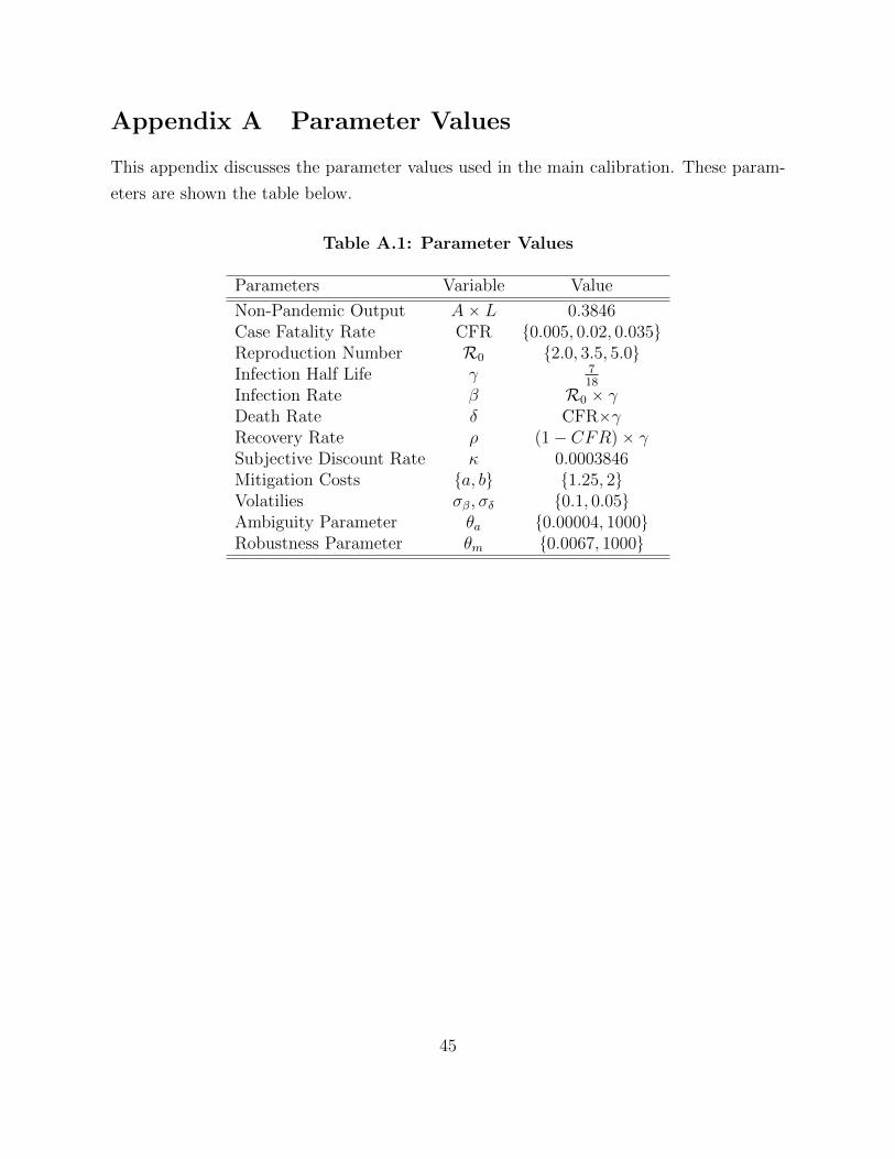
Appendix A Parameter Values

This appendix discusses the parameter values used in the main calibration. These param-

eters are shown the table below.

Table A.1: Parameter Values

Parameters Variable Value

Non-Pandemic Output Aˆ L 0.3846Case Fatality Rate CFR t0.005, 0.02, 0.035uReproduction Number R0 t2.0, 3.5, 5.0uInfection Half Life γ 7

18

Infection Rate β R0 ˆ γDeath Rate δ CFRˆγRecovery Rate ρ p1´ CFRq ˆ γSubjective Discount Rate κ 0.0003846Mitigation Costs ta, bu t1.25, 2uVolatilies σβ, σδ t0.1, 0.05uAmbiguity Parameter θa t0.00004, 1000uRobustness Parameter θm t0.0067, 1000u

45

Appendix B Numerical Solution Method

The numerical method we implement here has been used and developed in other papers,

including Barnett et al. (2019), and the summary of this algorithm that we provide here

closely follows what has been outlined in those papers15. We solve the HJB equations that

are given by nonlinear partial differential equations using the method of false transient

with an implicit finite difference scheme and conjugate gradient solver. The PDEs can be

expressed in a conditionally linear form given by

0 “ Vtpxq ` Apx;V, Vx, VxxqV pxq `Bpx;V, Vx, VxxqVxpxq

`1

2trrCpx;V, Vx, VxxqVxxpxqCpx;V, Vx, Vxxqs `Dpx;V, Vx, Vxxq

x is a state variable vector and Vxpxq “BVBxpxq, Vxxpxq “

B2VBxBx1

pxq are used for notational

simplicity. The agent has an infinite horizon and so the problem is time stationary. Thus,

Vtpxq “BVBtpxq has been added as a “false transient” in order to construct the iterative

solution algorithm. In particular, the solution comes by finding a V pxq such that the above

equality holds and Vtpxq “ 0.

The solution is found by first guessing a value function V 0pxq. Approximate derivativesĂV 0x pxq and ĂV 0

xxpxq are calculated from V 0pxq using central finite differences (except at the

boundaries where central differences require points outside the discretized state space and

so appropriate forward or backward differences are used). These derivatives are used to

calculate the coefficients A,B,C and D, and depend on the value function and its deriva-

tives because of the maximization from choosing optimal controls tik, iR, Nu in order to

maximize utility. Applying a backward difference for V 0t pxq, plugging in the calculated

coefficients to the conditionally linear system, and rearranging gives

V 1pxq “ V 0

pxq ` rApx, V 0, ĂV 0x ,

ĂV 0xxqV

0pxq `Bpx, V 0, ĂV 0

x ,ĂV 0xxq

ĂV 0x pxq

`1

2trrCpx, V 0, ĂV 0

x ,ĂV 0xxq

ĂV 0xxpxqCpx, V

0, ĂV 0x ,

ĂV 0xxqs `Dpx, V

0, ĂV 0x ,

ĂV 0xxqs∆t

We then solve numerically for V 1pxq and repeat this process, with the solution at each

iteration k serving as the guess for the next iteration k` 1, until maxx|V k`1pxq´V kpxq|

∆tă tol

for a specified tol ą 0. The choice of ∆t is made by trading off increases in speed of

convergence, achieved by increasing the size of ∆t, and maintaining stability of the iterative

15Joseph Huang, Paymon Khorrami, Fabrice Tourre, and the research professionals at the Macro FinanceResearch Program helped in developing the software for this solution method.

46

algorithm, achieved by decreasing ∆t.

The equation for V 1pxq can be expressed as a linear system Λχ “ π, whose solution

at each iteration is found by using the conjugate gradient method. This method uses an

iterative method to minimize the quadratic expression 12χ1Λχ´χ1π. The χ that minimizes

this expression is equivalent to the solution of the linear system if Λ is positive definite

as the first-order condition for the minimization problem requires Λχ ´ π “ 0. While my

Λ is not necessarily symmetric, because it is invertible we can transform our system to

Λ1Λχ “ Λ1π ðñ Λχ “ π which satisfies the necessary conditions and has the same

solution as our original linear system.

Table A.2 provides values used for the state space discretization and hyper-parameters

needed for the numerical algorithm used to solve my model. ∆t refers to the false tran-

sient step size referred to above, ε is the tolerance set for the false transient conver-

gence algorithm, ns, ni, nd are the discretization step sizes for the states variables, and

smax, imax, dmax, smin, imin, dmin are the maximum and minimum values for the discretized

state space.

An important numerical issue to consider in this framework is that the state space has an

important adding up constraint that 1 “ st ` it ` rt ` dt. We have limited the discretized

state space to focus on the relevant regions of each population to achieve an accurate

approximation, but we also limit the number of points where this adding up constraint

is violated. While various boundary condition methods can be used in cases where points

violate the adding up constraint, such as Dirichlet or reflective boundary conditions, we use

an interpolative Neumann boundary to approximate the derivative of the value function

at these points based on nearest points that satisfy the adding up constraint. We tried

various state regions to try to verify that our numerical framework provides consistent and

robust solutions.

Appendix C Uncertainty Through Robustness Results

This section provides additional robustness results, corresponding to the model presented

in section 6. We apply a slightly simplified version of the three scenario exercise done with

the smooth ambiguity model.

The first case we consider is a case in which models underestimate the severity of the

new disease. Here the planner assumes the pandemic has a lower R0 and CFR than is true.

The baseline model assumes R0 “ 2 and CFR“ 0.005, while the true model is R0 “ 5 and

47

Table A.2: Numerical hyper-parameters

FT step size ∆t 0.05Tolerance parameter ε 1e´ 12

s step size ns 0.0750i step size ni 0.0333d step size nd 0.0037

s max value smax 1.0i max value imax 0.4d max value dmax 0.03s min value smin 0.0i min value imin 0.0i min value dmin 0.0

CFR“ 0.035. This case is shown in Figure A.1. The results and intuition are very similar

to those shown in Figure 6 and discussed thereafter.

The second case we consider is a case in which models correctly estimate the severity of

the new disease. The planner’s assumed baseline model assumes R0 “ 3.5 and CFR“ 0.02,

which matches the true model. This case is shown in Figure A.2. Again, the results and

intuition are nearly identical to those shown in Figure 8 and discussed thereafter.

The third case we consider is a case in which models over estimate the severity of the

new disease. The planner here assumes the baseline pandemic model of R0 “ 5.0 and

CFR“ 0.035, while the true pandemic model is R0 “ 2.0 and CFR“ 0.005. This case

is shown in Figure A.3. As with the previous two cases, the results and intuition are

essentially identical to those shown in Figure 10 and discussed thereafter.

48

Figure A.1: Scenario 1: Underestimating the Pandemic

Notes: These figures show (i) the prior model response (red), the true optimal response (black), and the

uncertainty-adjusted response (blue) in the case where the policy maker initially underestimates the severity

of the pandemic. From left to right, top to bottom, these figures are (1) the fraction of the population

that is susceptible to the disease, (2) the fraction of the population that is infected, (3) the fraction of the

population that has had the disease and recovered, (4) the fraction of the population that has died, and (5)

the fraction of the population in quarantine. 49

Figure A.2: Scenario 2: Correctly Estimating the Pandemic

Notes: These figures show (i) the prior model response (red), the true optimal response (black), and the

uncertainty-adjusted response (blue) in the case where the policy maker initially correctly estimates the

severity of the pandemic. From left to right, top to bottom, these figures are (1) the fraction of the population

that is susceptible to the disease, (2) the fraction of the population that is infected, (3) the fraction of the

population that has had the disease and recovered, (4) the fraction of the population that has died, and (5)

the fraction of the population in quarantine. 50

Figure A.3: Scenario 3: Overestimating the Pandemic

Notes: These figures show (i) the prior model response (red), the true optimal response (black), and the

uncertainty-adjusted response (blue) in the case where the policy maker initially overestimates the severity

of the pandemic. From left to right, top to bottom, these figures are (1) the fraction of the population

that is susceptible to the disease, (2) the fraction of the population that is infected, (3) the fraction of the

population that has had the disease and recovered, (4) the fraction of the population that has died, and (5)

the fraction of the population in quarantine. 51