1126 E. 59th St, Chicago, IL 60637 Main: 773.702.5599

bfi.uchicago.edu

WORKING PAPER · NO. 2018-32

Occupational Licensing and Accountant Quality: Evidence from the 150-Hour Rule

John M. BarriosMay 2018

Occupational Licensing and Accountant Quality:Evidence from the 150-Hour Rule

John M. Barrios∗

University of Chicago Booth School of Business

April 23, 2018

Abstract

I examine the effects of mandatory occupational licensure on the quality of Certified

Public Accountants (CPAs) using the staggered state-level adoption of the 150-hour

Rule (the Rule). Although the Rule reduces the number of entrants into the profession,

an analysis of labor market outcomes shows that accountants subject to the Rule are

more likely to be employed at a Big 4 public accounting firm and specialize in taxation.

However, accountants subject to the Rule have the same likelihood of promotion, the

same duration until promotion, and exit public accounting at faster rates than their

non-Rule counterparts. Moreover, Rule accountants earn a wage premium relative to

non-Rule accountants. These findings suggest that restrictive licensing laws reduced

the supply of new CPAs and increased rents to the profession without drastically

improving quality in the labor market.

Keywords: The 150-Hour Rule, Occupational Licensure, CPA Licensure, Screening, Human

Capital, Labor Market Outcomes, Hazard Rate Model.

JEL Classification Numbers: D45, I21, J2, K2, L51, M4.

∗Address: University of Chicago Booth School of Business, 5807 South Woodlawn Ave. Chicago, IL60637, phone: 773-702-1268, e-mail: john.barrios@chicagobooth.edu.

This paper is based on my dissertation at the University of Miami, School of Business Administra-tion. I am grateful for the invaluable comments and suggestions provided by my co-chairs DhananjayNanda and Andrew Leone as well as fellow committee members Peter Wysocki and Laura Giuliano. Iwould also like to express gratitude to seminar participants at Duke, MIT, Temple, University of Alberta,UCLA, University of Chicago Booth, University of Miami, University of Rochester, University of TexasDallas, and AEA Chicago. Any errors in the paper are my own. Previously titled ”Accountant Quality”and ”Occupational Licensing and Accountant Quality: Evidence from LinkedIn”.

1

1 Introduction

The quality of corporate financial reporting is of central importance to capital market partic-

ipants, regulators, and scholars. The demand for audits (as well as regulation of accounting

and auditing standards) arises from information asymmetries that exist between manage-

ment and financial statement users. Without independent audits, management could exploit

its information advantage and misrepresent the firm’s underlying economic performance. As

a result, the regulation of financial reporting and auditing services has been one of the most

widely examined topics in the accounting literature.1 However, the quality of independent

audits is a function of not only the quality of auditing standards established by regulators

and the quality of procedures established by accounting firms based on these standards, but

also the quality and expertise of the accountants responsible for the audits.

Given the vital role that auditors play in assuring financial reporting quality, the emer-

gence of occupational licensing requirements (e.g., the CPA exam, educational requirements,

and experience requirements) for those conducting audits (i.e., Certified Public Accountants

or CPAs) is not surprising.2 It is somewhat surprising, however, that there is a paucity of

evidence on the effects of licensing requirements on the quality and preparation of those who

select into the accounting profession. In this paper, I take a first step to fill this void by

examining the effect changes in the restrictiveness of licensing requirements of CPAs have

on the supply and quality of those who enter the accounting profession.

The minimum educational requirement for CPA licensure has historically been 120

semester hours of college course work, typically completed in four years. Approximately

four decades ago, the accounting profession began debating the advantages of implementing

a 150-semester-hour requirement for licensure. The stated objective of this requirement was

to enhance the quality of work performed by CPAs by bringing better CPAs into the profes-

1For reviews, see DeFond and Zhang (2014) and Francis (2011).2The rationale for such regulation is that it helps avoid negative third-party effects that may result from

incompetent practitioners. For example, the licensing of CPAs is rationalized, in part, as protecting investorswho must rely on the accuracy of financial information produced and verified by accountants who are neitherselected by, nor accountable to investors.

2

sion (Elam (1996)). The 150-hour requirement (hereafter, the Rule) has now been adopted

and is in force in all 54 U.S. jurisdictions. My analysis relies on the Rule’s staggered adoption

to provide insight into the effects of increases in licensing restrictiveness on the individuals

who prepare and audit financial statements.

The relation between licensing rules and outcomes is not without significant tension. Pro-

ponents of professional licensure justify these laws as a means to protect the public against in-

competent, unprepared, or irresponsible practitioners (Kleiner (2000); Leland (1979)). From

this public-interest view of licensing asserts that administrative procedures regulate the qual-

ity of labor in the market. The regulator screens entrants to the profession and bars those

whose skills or character traits suggest a tendency toward low-quality output, thus raising the

lower tail of the quality distribution and providing a minimum guaranteed level of quality and

safety to consumers. This public-interest perspective, the Rule, with its additional 30 credit

hours of education, arguably serves as a screening mechanism to separate high-ability CPAs

from low-ability CPAs through their willingness to acquire the additional education. Thus,

if the public-interest view motivates the Rule’s implementation, the quality of individuals in

the profession should be raised via a reduction in the supply of candidates.3

On the other hand, critics of professional licensure argue that licensing merely secures

higher rents for those in the occupation, by raising prices and, in particular, harming con-

sumers who may not be able to afford their preferred level of service. This capture/private-

interest perspective views licensing as mainly a rent-seeking barrier to entry introduced by

current members of the profession to limit the supply of new entrants and extract monopoly

rents (Friedman (1962); Stigler (1971); Maurizi (1974)). This view of licensing predicts that

the Rule reduces the number of entrants while maintaining the average candidate quality or

even deteriorating the quality if the incremental time cost of the Rule leads to high-ability

students switching to other disciplines because of their higher opportunity cost of time.

Moreover, in addition to the null quality effects, this hypothesis predicts an increase in rents

3The Rule’s required additional education could have a human capital effect with individuals investingin more schooling irrespective of its supply effects.

3

for grandfathered CPAs after the Rule’s adoption.

The main obstacle in studying CPAs’ labor market outcomes is a lack of available data on

individuals’ employment and education histories. Available empirical measures of aggregate

job-to-job and cross-industry transitions in the labor literature are typically constructed us-

ing census data.4 Yet, using census data for accounting professionals stretches the limits of

the surveys given their low coverage of accounting professionals and their inability to disen-

tangle CPAs from bookkeepers. Moreover, previous studies in accounting rely on National

Association of State Boards of Accountancy (NASBA) data to examine the supply effects

of the Rule (Jacob and Murray (2006)). While these studies find reductions in the number

of candidates sitting for the exam, they do not provide direct evidence of the Rule’s quality

effects given the limitations of the data. I circumvent this challenge by constructing a new,

comprehensive panel dataset of career paths for more than 10,000 CPAs from 11 states who

post their resumes on a major professional networking website. My sample spans the past

four decades and provides a unique overview of the individual CPAs’ employment and ed-

ucational histories that allows me to examine differences in the labor market outcomes of

CPAs who are subject to the Rule against those who are not. Specifically, I measure average

tenure, number of positions, time until promotion, and time in public accounting for each

individual. These measures allow for explicit tests of the quality of CPAs on the full sample

of CPAs as well as on a matched sample where CPAs subject to the Rule are matched based

on graduation year and gender to non-Rule CPAs.

I begin my analysis by using an extensive panel dataset of first-time CPA test takers

from NASBA for the years 1984–2004 to reexamine changes in the supply of CPA candi-

dates. Using a difference-in-differences specification, I find a 15% reduction in the number

of candidates taking the exam for the first time following the Rule’s enactment. Yet, the

decrease does not come solely from the low end of the distribution but also from the upper

tail. High type candidates’ higher opportunity cost of time leads to fewer taking the exam

4Labor studies typically use the Current Population Survey (CPS), the Survey of Income and ProgramParticipation (SIPP), or the Panel Study of Income Dynamics (PSID).

4

after the Rule. Thus, while the Rule increases the marginal cost of becoming a CPA, it is

unclear to what extent the quality of the labor market changed given the reduction in both

high and low types. As a result of this ambiguity, I use individuals’ labor market outcomes

to examine the Rule’s long-term quality effects.

Descriptively I find that the Rule had an effect on the employment focus of CPAs, such

that Rule CPAs are comparatively more likely to be employed at a Big 4 public accounting

firm, are more likely to specialize, and are more likely to have more graduate degrees. With

respect to quality effects, I find no significant difference in the time until promotion between

the two groups. Furthermore, I find that CPAs subject to the Rule spend a larger percentage

of their careers in public accounting although they tend to exit public accounting at higher

rates than their non-Rule counterparts. Five years into their careers 62% of the Rule cohort

have left public accounting as compared to only 59% of the non-Rule cohort. Assuming

that promotions and tenure length are measures of CPA quality, the lack of a significant

difference between Rule and non-Rule individuals in promotions and tenures casts doubt

on the Rule’s screening role and the public-interest motivation for the Rule. The breadth

of options with which the requirement can be fulfilled (e.g., a master’s degree or separate

courses) likely allow some low-ability CPAs to pass the screening via non-degree programs

and thereby diminishes the screening value of the Rule.

The null effect on quality does not necessarily support the capture/private-interest view

of licensing. To provide evidence of rent extraction, I use data from the current population

survey to examine the Rule’s effect on wages. I examine whether accounting professionals

in states that adopted the Rule collect rents above what can be explain by their education.

Using a difference-in-differences specification, I document a 9% earnings premium for CPAs

in Rule states relative to equally educated CPAs in non-Rule states. Collectively, I document

that while the Rule decreased supply, it did not lead to an increase in average quality while

still increasing rents to the profession. This is consistent with my inferences of the dominant

role that the capture/private-interest view played in the adoption and implementation of the

5

Rule.

I conduct an array of robustness and sensitivity tests to validate my inferences. In

particular, I address whether noise in the classification of job titles drives the promotion

results, by focusing only on those individuals who become partners and testing for differences

in their time until promotion to partnership. Using the sample of CPA partners, I also find a

insignificant difference in the time until promotion between the Rule and non-Rule cohorts.

This reinforces earlier findings of insignificant differences in long-term performance.

I also evaluate whether noise in the overall resume data can explain my quality findings

that would make a null result more likely. To test the impact of data quality, I examine dif-

ferences between CPAs with and without a master’s degree. Prior literature has documented

a significant difference in outcomes for master’s degree holders (Arrow (1973); Spence (1973);

Card (1999); Dupray (2001)). When I rerun my tests on master’s versus non-master’s degree

holders, I find that master’s degree holders spend less time in each position, have more jobs,

and are promoted at faster rates. This finding alleviates concerns about power in the tests

and further confirms the benefits of a graduate degree.

My study is subject to several caveats. The long-term labor market outcome measures

in this study rely on individuals being promoted based on some quality differential. Thus,

my tests are limited to the extent that promotions in firms do not incorporate quality.

Additionally, inferences based on resume data are subject to concerns about selection and

accuracy given the voluntary nature of the profiles and the reporting errors or biases that

may be present in the resumes. The pervasive use of the website by individuals for credible

networking, as well as job-search purposes, however, provides some assurance as to the

integrity of the data posted. Moreover, unlike lying on a resume, which only a prospective

employer will see and cannot easily verify, lying on one’s profile is publicly visible. This

public accountability makes it more difficult for individuals to make false claims about their

employment and is thus distinct from traditional resume data. Yet, despite such potential

limitations, the data allow me to document some of the first large-scale evidence on the

6

long-term labor market outcomes of CPAs.

This paper makes several contributions to the literature. First, it provides a comprehen-

sive examination of the Rule’s effect on the accounting labor market as well as an evaluation

of licensing’s effect on CPAs’ quality. Despite the Rule being in effect in all 54 U.S. juris-

dictions, to date there has been no long-run analysis of the Rule’s effect on the individuals

entering the accounting profession. While previous studies have mostly been normative in

their assessments of the benefits of the Rule, I provide a positive cost-benefit analysis of the

Rule’s impact. Second, this paper provides a foundation for more research that connects

labor economics to the accounting literature, by utilizing insights from personnel economics

and human capital to improve our understanding of disclosure production and audit quality.

For example, Francis (2011) suggests that “audits are of higher quality when undertaken by

competent people.” Yet, most extant research examines audit-firm or office-level characteris-

tics and, due to a lack of data, implicitly assumes that there is little within-firm heterogeneity

. Moreover, while the debate about the regulation of disclosure and auditing continues to be

contentious, it is critical that we consider the individuals who implement these standards in

order to fully understand the full effects of the regulated standards.

Finally, this paper contributes to the broader literature on occupational licensing and

education. Occupational licensing regulation affects nearly 30% of the U.S. labor force, a

larger proportion of workers than are in unions or covered by minimum wage laws ( Kleiner

and Krueger (2010)). Given its breadth, occupational licensing has begun to be scrutinized.

A recent Wall Street Journal article highlighted the fact that the Obama administration

budgeted $15 million to study the costs and benefits of occupational licensing on the U.S.

labor market(Litan (2015)). The Rule’s supply restriction, its increase in rents, and the lack

of a quality effect further cast doubt on the effectiveness of increases in licensing restrictions

in the labor market. Additionally, the stringency of mandatory educational requirements

for licensing has also begun to be called into question in professions such as medicine and

law. For example, the cost of law school has been framed as a major impediment to getting

7

underrepresented minorities into law (Rodriguez and Estreicher (2013)). Moreover, there

have been recent calls to reduce the required years of law school from three to two years

(Estreicher (2012)). In medicine, the relative costs and benefits of a fourth year of medical

school have also been called into question given the scarcity of new medical students and the

increasing demand for medical services in the near future (Emanuel and Fuchs (2012)). Using

the Rule, this paper sheds light on the reasonableness of reducing the number of mandated

school years for other professions to increase access to the profession while still maintaining

quality.

The remainder of the paper is structured as follows. Section 2 provides the Rule’s insti-

tutional background and the economic framework used to analyze individuals’ labor market

outcomes. Section 3 presents my data sources and sample selection procedure, and describes

the data. Section 4 presents the empirical analysis and provides a series of sensitivity tests

and robustness checks. Section 5 concludes.

2 Institutional Background and Economic Framework

2.1 Licensing of Accountants and the 150-Hour Rule

Occupational licensing regulation specifies the requirements a practitioner must fulfill in or-

der to be permitted to perform certain services. Such regulation currently governs more than

one thousand occupations (Brinegar (2006)) or nearly thirty percent of the U.S. workforce.

Additionally, over the past several decades, both the number of occupations and the per-

centage of the workforce covered by such regulations have increased dramatically (Kleiner

and Krueger (2013)). These, mostly state-level, regulations directly affect both blue- and

white-collar workers.

In the accounting profession, the CPA license entitles an individual to audit firm financial

statements and attest to their compliance with generally accepted accounting principles

8

(Jacob and Murray (2006)).5 Non-holders are not legally permitted to undertake this activity.

Currently, state boards of accountancy have put in place educational, experience, ethics, and

national examination requirements that must be satisfied in order for accountants to practice

legally in state and local jurisdictions as CPAs. While all CPA applicants are required

to pass the national CPA examination set by the American Institute of Certified Public

Accountants (AICPA), the Rule required that these applicants to complete 150 semester

hours of additional education prior to obtaining their license.

The AICPA spent the past century wrestling with ways in which to elevate the prestige of

the profession through higher education (Van Wyhe (1994)).6 Yet, it was not until the 1980s

that the AICPA finally institutionalized an extended educational curriculum for licensure,

driven by an increase in congressional scrutiny over several prominent audit failures.

The savings and loan crisis of the 1980s gave way to a series of congressional hearings

regarding the role of auditors in the crisis. The hearings examined how several prominent

public companies, ranging from the Penn Square Bank in Oklahoma to E.S.M. Securities

in Florida, failed so soon after receiving clean audit opinions (Berg (1988)). The threat of

congressional scrutiny, with regard to new federal regulation on the accounting profession, led

the AICPA in the mid-1980s to implement a set of reforms in the name of “self-regulation”

(Madison and Meonske (1991)). One of the main tenets of these reforms was to require CPA

candidates and AICPA members to have 150-semester hours of college education prior to

receiving membership (Committee (1986)). In 1988, at its annual meeting in New York City,

84% of the AICPA’s voting members backed the proposal, effective for the year 2000. The

AICPA asserted that the requirement was meant to “improve the overall quality of work

performed by CPAs” and “ensure the quality of future audits” by improving the quality of

audit staff and those entering the profession (AICPA (2003)).

5These individuals also enjoy various privileges before the Internal Revenue Service.6As early as 1937, the governing council of the American Institute of Accountants (AIA), superseded

by the AICPA, publicly stated that the “highest practicable standards of preliminary education similar tothose effective in other professions, such as law or medicine” should be required for the accounting profession(Allen and Woodland (2006)).

9

While the AICPA required the Rule for membership, the state boards of accountancy

would have to adopt the Rule in order for it to be legally required for licensure. While states

like Florida and Hawaii adopted the Rule as early as 1979, the majority of the state boards

began passing the Rule only after the AICPA’s action. Relying on the AICPA’s assertions,

state boards of accountancy began adopting the requirement as a condition for CPA licensure

in the mid-1990s and early 2000s. In the year 2000 alone, 14 states adopted the Rule (see

Table 1 for details on the Rule’s years of adoption and enactment).

Yet, even before the adoption of the Rule, most jurisdictions already specified a minimum

number of hours in business and accounting. Moreover, most states did not change these

detailed requirements with the adoption of the Rule.7 The Rule, which required 150 semester

hours rather than a master’s degree, was worded in order to provide flexibility to colleges

and universities in designing their programs.8 Specifically, this freedom was granted in

order to allow four-year colleges, which do not have the authority to grant master’s degrees,

the ability to offer programs that could meet the Rule’s requirement (Jacob and Murray

(2006)).9 As a result, candidates for the CPA exam could accumulate the additional hours

of education through courses associated with a graduate degree (an MBA with an accounting

concentration or a master’s in accounting), courses from another upper-level undergraduate

option (a second major), or courses from no specified program of study at all.10 As of July

2017, the Rule has been enacted in all 54 U.S. licensing jurisdictions, with the states of New

Hampshire, California, and Vermont beginning enforcement in 2014 and Colorado in 2015.

7The AICPA pushed for the extra 30 credit hours to be composed of more general liberal arts courses aswell as general business courses rather than pure accounting ones (Collins (1989)).

8In this regard, the Rule has been criticized for allowing CPA candidates to meet the requirements forlicensure with no more hours in business and accounting than what was already required under the oldregulations.

9The political economy of the Rule can be seen in the case of Oklahoma where the original bill thatrequired graduate courses to fulfill the Rule was not passed after lobbying by four-year universities. The billeventually passed when the wording was changed to 30 additional hours of higher-level education.

10See Online Appendix A for a list of the current educational requirements by state.

10

2.2 An Economic Framework for the Rule

This section provides a discussion of previous theoretical and empirical work on occupational

licensing in order to motivate my analysis of the Rule’s effect on the supply of labor into

the profession and its quality. Despite the fact that occupational licensing covers 30% of the

U.S. workforce, its effects on the supply and quality of professionals is not without tension

(Kleiner and Krueger (2013)).

The traditional motivation for occupational licensing stems from the public-interest view

of licensing, which asserts that licensing is needed in cases of imperfect information to protect

consumers (Shapiro (1986)). Theoretical work along this line claims that credence goods

such as attestation demand regulation on the basis of quality certification (Leland (1979)

and Shapiro (1986)). In the absence of regulation, consumers, it is alleged, will tend to

drift to the low-price, low-quality alternative. This perspective suggests that administrative

procedures from regulators (i.e., state boards) regulate the supply of labor in the market.

The regulator screens new entrants to the profession and bars those whose skills or character

traits suggest low-quality outputs (Gittleman and Kleiner (2013)).The imposition of licensing

in such markets may in effect shift the quality-adjusted demand curve upward, improving

consumer welfare and increasing the supply of such services by ensuring that only high-

ability individuals perform the tasks (Adams III et al. (2003)). In the case of the Rule, the

willingness of the individuals to undertake the additional 30 hours of course work should

be correlated with increased ability and high quality (Spence (1973)). Moreover, the extra

year of education required under the Rule can also be viewed as an additional investment

by individuals in their human capital that will lead to increases in the quality of these

individuals irrespective of the restrictions on entry (Becker (1993)). Thus, the public-interest

view predicts that the supply of CPAs will be lowered by the Rule, but that this decline in

supply will represent a decrease in low types and as a result increase the average quality of

individuals in the market.

In contrast to the public-interest motive, a capture/private-interest motive for licensing

11

has been suggested by a large stream of literature in regulatory economics, whereby changes

in licensing requirements are introduced by current members of the profession to limit the

supply of new entrants and extract monopoly rents (Friedman (1962); Stigler (1971); Maurizi

(1974)).11 On the one hand, it predicts that the Rule’s additional 30-credit hour requirement

will increase the marginal cost of becoming a CPA and reduce the number of new CPAs as

in the public-interest case, but, on the other hand, it holds that the average quality of

candidates in the market will remain unchanged or even be reduced.12 For example, the

variety of ways in which to meet the 30-credit-hour requirement of the Rule could make it

ineffective in filtering out low types as the requirement may not be less costly to high types.

The approximate one-year increase in the necessary time to complete the Rule’s educational

requirement could potentially lead to adverse selection by high-ability potential CPAs. Their

relatively higher opportunity cost of time could force them into substitute fields as a result

of the additional year (Akerlof (1970)). This in turn would lead to a decrease in the overall

quality of CPAs after the implementation of the Rule. Along this line of reasoning, Lee

et al. (1999) analytically incorporate auditors’ education and audit effort as joint inputs of

audit quality in a Dye (1993) and Dye (1995) model to evaluate the effects of the Rule on

the audit market. They show that the audit fees are higher, making pre-Rule CPAs better

off and audit clients worse off as a result of the compositional supply changes to the Rule.

Finally, the capture/private-interest view predicts that the reduction in supply will lead to

increases in rents by the profession. By restricting the supply of CPAs, the Rule will allow

the profession to increase their rents (Kleiner (2006) ; Kleiner and Krueger (2013)). As a

result, the capture/private-interest view will be supported if we observe reductions in supply

and increases in rents that are not accompanied by increases in quality.

11The use of licensing raises the entry costs into a profession by imposing a fee as well as training require-ments, which shift the short-run and long-run supply curves upward and left (Maurizi (1974)).

12Several studies have provided empirical evidence on the supply reducing effects of occupational licensurein other occupations (Shepard (1978) and Carroll and Gaston (1981)).

12

3 Data

3.1 Samples

This section introduces the data from both the business networking website and my other

sources. My primary empirical analysis requires (i) candidate data from the CPA exam, (ii)

education and employment histories for a sample of CPAs, and (iii) wage data on individ-

uals in accounting. My analysis of CPA quality relies on data from a leading professional

networking website that includes the self-reported resume of each user. My supply and rent

extraction tests rely on data from NASBA and the Current Population Survey.

Business Networking Website Data The professional networking website (hereafter

referred to as the “website”) serves as the world’s largest online professional networking and

recruiting site. The website began as a networking site for technology and financial industry

employees and has grown tremendously ever since. It now covers various industries and

has members at all levels of experience, i.e., from college students to senior executives.

As of 2014, the website includes executives from all Fortune 500 companies as members.

Additionally, its members represent a vast array of age groups: 46% of members are between

the ages of 25 and 44 while 35% are between the ages of 45 and 64. With respect to the

accounting profession, the website lists over 656,000 CPAs in the continental United States,

roughly 60% of the number of individuals estimated by the Bureau of Labor Statistics to be

in the occupational category of accounting (of Labor Statistics (2018)). Given the breadth

of coverage, the site serves as an effective data source for information on CPAs, including

their education and career outcomes.

For the purposes of the present study, computational restrictions on the data collection

process limit my study to a sample of individuals drawn from 11 prominent states. The 11

states were chosen by their relative importance in terms of the number of accountants, their

contribution to the national GDP, and their relative timing in the enactment of the Rule.

Table 2 provides a descriptive overview of the characteristics of the 11 states analyzed in the

13

study.

I begin the construction of my sample by searching for individuals who either self-report

“CPA” or “Certified Public Accountant” on their profiles. The website search is restricted

neither by geographical proximity nor by the personal connections of the account used to

search. On a state-by-state basis, I draw individuals who entered the labor market (i.e.,

obtained their CPA) around the enactment of the Rule.13 To understand the sample size

considerations, I conducted several power calculation tests. The goal of a power test is to

identify sample sizes required to detect a pre-specified treatment effect (minimum detectable

effect) at specified levels of power and statistical significance. In my case, as is consistent

with common practice, I consider sample sizes for a specified power of 0.8 and a statistical

significance of 0.05.14 The results of the power test support the following: if I can obtain 1200-

1500 individuals into both the treatment and control groups, I will likely be able to detect

an effect that represents between a 10–25% change from the baseline rate of the controls.

The large minimum detectable effect also takes into account the potential for cross-over (i.e.,

the possibility that I misclassify treated Rule CPAs as controls) of approximately 15%. As

a result, I collect an initial sample of 2,500 individuals per state to ensure sufficient power

in my tests.

Based on the selected profiles, I collect workers’ information, focusing in particular on

the career path of each individual. For each position, I observe the job title held by the

individual, the start and end dates for each job title, and the company name. The job titles

and descriptions for a given position allow me to classify jobs based on seniority in order

to decipher promotions versus lateral changes for individuals. I determine the chronological

order of the positions using their arrangement on the profile page, and assign to each worker

a unique identifier. I also collect data on the user’s gender and current location. I perform

13The collection process requires that I screen the profiles afterwards to make sure I capture CPAs andnot individuals that list CPA in descriptions of work-related projects such as accounting software in an ITfirm.

14The power calculations require estimates of variances for treated and control samples. In experimentalsettings, these are obtained from pre-existing data or acquired from a pilot study. Since I did not have eitherwhen I was planning the paper, I made additional assumptions on reasonable estimates for these values.

14

additional data cleaning by using an individual’s unique ID to remove duplicate individuals

that may arise due to the automated collection of the profiles. I reshape the data in the

resume, which is reported at each job level to a panel that lists an individual’s name and

work information in each period.

A key issue that I face is multiple overlapping job spells; that is, some individuals may

list several occupations over the same period. While I track all occupations for all the

individuals in the sample, I need to make some assumptions when conducting the analysis

of career transitions. In particular, I limit my analysis to individuals who list a maximum

of two simultaneous occupations in a year. These individuals account for more than 90%

of my original sample. In order to deal with missing spells or holes in resumes, I classify

an individual as unemployed if there is a one- or two-year-long time gap between job (or

education) spells and, on the other hand, classify a spell as having missing information if

the time gap between two spells is longer than two years.

A critical variable for labor market outcomes is an individual’s age. As age is not ex-

plicitly included in the resume, I determine an individual’s age in a given period under

the following rule: (i) age at high school graduation is 18 plus any years of prior full-time

employment, (ii) otherwise, age for starting a college degree is 18 plus any years of prior

full-time employment, (iii) otherwise, age at completing an Associates Degree is 20 plus any

years of prior full-time employment, (iv) otherwise, age for completing a Bachelor’s Degree is

22 plus any years of prior full-time employment. I consider 3-year college degrees (typically

from international institutions) to be equivalent to bachelor’s degrees. In addition, given

the sample considerations, I place associates degrees with high school graduates. Finally,

I distinguish between the following graduate degrees: masters, juris doctor (JD), masters

of business administration (MBA), master’s of accounting, and PhD. I assume that missing

education signals a high school graduate or less. Missing education also implies missing age

since I infer an individual’s age based on education dates. In such cases, instead of age, I

match years since first work experience.

15

Finally, in order for a profile to be included in the sample, I require that it contain

educational information, such as university attended, degree obtained, and/or graduation

year. In addition to the education, I require it to have a complete career history with job

titles and dates. Appendix A provides a descriptive table on the sample selection data

requirements and changes in the sample. In the end I am left with a sample of over 10,000

CPAs with clean work experience and 8,793 individuals with complete education.

I believe that the extensive amount of collected data, and descriptive evidence suggest

that my sample represents a reasonably accurate collection of CPAs. That said, despite my

efforts to collect, clean, and validate the data, it is unlikely that I have accurately identified

all individuals and their backgrounds for all of my sample. This is the result of three different

issues: (1) individuals not registering their resumes on the professional networking website,

(2) individuals potentially either omitting or incorrectly listing information on their profiles

(preventing me from accurately pairing them to years, identifying prior work experience, or

capturing their education and training), and (3) errors in my collection and parsing of these

profiles. With respect to reporting biases and errors, inferences based on resume data in

general are subject to these concerns given the voluntary nature of the profiles. Yet, the

pervasive use of the website by individuals for credible networking, as well as job search

purposes, provides some assurance of the integrity of the posted data. Moreover, unlike

lying on a resume, which only a prospective employer will see and cannot easily verify, lying

on one’s profile is publicly visible. This public accountability makes it more difficult for

individuals to make false claims about their employment and is distinct from traditional

resume data. Despite efforts to reduce these risks, my inferences should be interpreted with

these caveats in mind.

Additional Data Sources My CPA supply analysis relies on data from NASBA.

NASBA provides data on the number of first-time candidates, repeat candidates, and total

candidates for each of the exam periods by jurisdiction from 1984–2014. At the university

level, I obtain data on the total number of first-time test takers as well as the number of

16

individuals who pass all four sections in one sitting and the number of individuals who fail

all four sections.

Data for my tests on CPAs’ rent extraction comes from the CPS. The CPS has gathered

employment and demographic data from 57,000 households on a yearly basis since 1988 to

represent the nation as a whole. Employment information for individuals participating in

the CPS is based on their occupation and industry. Thus, I select individuals who listed

Occupation Code 023, Accountants and Auditors, and Industry Code 089, Professional Ser-

vices.15 Additionally, those who did not report positive earnings were dropped from the

sample, resulting in a final sample of 6,994 accounting-related individuals. Finally, since

data is collected over various years, earnings are converted to 2010 dollars, using the Bureau

of Labor Statistics implicit price deflator.

3.2 Labor Market Outcome Variables

In order to examine quality differences between Rule and non-Rule CPAs, I construct non-

monetary proxies of labor market outcomes from labor economics and include proxies that

where proposed by advocates and critics of the Rule.16 I describe and motivate below the

measures of long-term labor market outcomes, which I build and use in my tests.

Number of Firms & Tenure I use the job titles and individual firm names to obtain

an accurate count of the individual’s positions during his or her career. The career histories

allow me to measure the individuals’ tenure at each firm as well as the total number of jobs

held. My examination of tenure at firms and turnover follows from economic theory and

arguments put forth by supporters of the Rule. Advocates of the Rule justified its imple-

mentation as a mechanism to reduce turnover at firms. Moreover, if the Rule had a human

capital effect, such as individuals taking additional classes, recent literature in human cap-

15It is unlikely that my sample solely includes CPAs. However, my selection criteria are as finely tunedas the census data permits with respect to pinpointing certain professions. It is also not unreasonable tobelieve that non-CPAs in the sample who work in close proximity to CPAs are also indirectly affected bythe occupational regulation of CPAs.

16These outcomes were advocated by industry leaders such as J.Michael Cook in his 1996 article “150-HourEducation Programs: A Practitioner’s Perspective on Useful Research Possibilities.”

17

ital has proposed that increases in human capital may lead to lower employment turnover.

Acemoglu and Pischke (1999) model increases in general human capital as increasing firm

productivity through firm-specific skills via complementarities in production. In their frame-

work, any increase in human capital by the Rule would lead to mobility constraints. As a

result, I investigate whether the Rule’s additional education requirement worked to improve

matches between individual CPAs and firms. If it had such an effect, as claimed by it ad-

vocates, one would then see a lower number of firms, all else equal, and longer tenures for

individuals at the firms.

Time till Promotion The length of time it takes individuals to be promoted should

serve as an attractive measure of ability in the absence of compensation. My focus on

time till promotion stems from the view that promotions serve to screen employees up the

organization and can thus be thought of as a screening mechanism in the internal labor

market of the firm. During the pre-promotion period the employee is trying to signal her

type with regard to her ability to perform higher-order tasks. As such, the timing until

selection for promotion can be seen as part of the screen, as it is being used by the firm to

decipher an individual’s type. Thus, time to promotion is a function of the underlying labor

pool quality, which means that promotion times should be shorter for high quality labor

pools and longer for low-quality labor pools.

If the Rule effectively screen high types, one would expect Rule individuals to reach

higher-level positions quicker than non-Rule individuals.17 In order to determine time until

promotion, I rely on job titles in the constructed database. The use of job titles stems

from the inability to observe wages or a systematic classification of job types with respect

to seniority/prestige. Specifically, I classify the job titles in the dataset into a three-tier

hierarchy meant to represent the job’s level of seniority. Then I take the job titles in the

17I believe it is helpful to distinguish between the likelihood of promotion and my duration (time tillpromotion) measure. In the case of likelihood of promotion, a relative performance evaluation would lead tono change in the expected likelihood of promotion if all individuals were subject to the Rule and the firmneeded to promote someone. By contrast, my focus on time till promotion does not rely on the likelihoodof promotion as I examine only individuals who get promoted in order to observe changes in the time untilpromotion.

18

dataset and match them based on similarity scores to the titles in a dictionary of titles with

seniority/prestige classifications from the Department of Labor as well as several online job

search engines. The seniority levels are meant to capture jobs that entail a higher level of

responsibility and wage rate. Their use allows me to disentangle promotions from lateral

moves.18

Time in Public Accounting My focus on the time individuals spend in public ac-

counting stems from its prominent use as a motivating factor for the Rule’s passage (Cook

(1996)). One of the main themes in arguments for the Rule’s enactment was its supposed

ability to increase the retention of CPAs in public accounting. It was suggested that by

screening higher-type CPAs the profession would be able to stop the exit of CPAs from

audit firms to clients. Moreover, even if the Rule were to lead to human capital accumula-

tion that makes Rule CPAs’ outside options more lucrative, their exit would lead to lower

audit quality. Using the detailed career history of individuals, I measure the length of time

individuals spend in public accounting. I construct this measure using a combination of

individuals’ job titles and the name of the firms in which they are employed to determine

the specific year in which they exit public accounting for the private sector.

3.3 Descriptive Statistics

3.3.1 Sample Descriptives: NASBA

Descriptive statistics for the NASBA sample are reported in Table 3. The table reports

sample means and medians for the number of first-time candidates at the university level

for the years 1984–2004. In addition to the total number of test takers, the table includes

the number of candidates passing (Passed All) and failing (Passed None) all four sections

of the CPA exam. Descriptive statistics for the Rule and non-Rule subsamples are also

provided. The average number of candidates per sitting is 20 at the university level with 3.5

18Appendix B provides a sample of the job titles that fall into each of the three tiers as well as descriptivestatistics on relative rank of seniority jobs in individuals’ careers and average tenure in each rank.

19

on average passing all four sections of the exam and 10.9 on average failing all four sections.

A comparison of the Rule and non-Rule subsamples indicates a decrease in the total number

of candidates sitting for the exam. The average number of test takers drops from 21.7 in the

non-Rule period to 15 in the Rule period. While this decline is reflected in the Passed None

number (which drops from 11 to on average 7), it is also evident in the Passed All number

(which drops from 3.75 to 2.87 on average). This decline in the Passed All number will be

formally analyzed when I examine the treatment effect of the Rule on the supply of CPAs

below.

3.3.2 Sample Descriptives: CPA Sample

In Table 4, Panel A, I provide descriptive statistics for my CPA sample of 8,793 CPAs along

the lines of demographics, career outcomes, and educational background. The sample is

skewed on gender with 61% of the sample being male. On average, individuals have 5.3

jobs during their career, averaging 4 years per job with 63% of the sample being employed

at a Big 4 public accounting firm at one point in their career. Twenty-one percent of the

sample has worked in taxation, and the mean graduation year in the sample is 1997. More

than 50% of the sample have master’s degrees with 25% of those degrees being specifically in

accounting. In addition to the sample averages, I also report changes in the means between

the non-Rule and Rule cohorts. Looking at the full sample, Rule individuals graduate 13

years later than non-Rule individuals, have more master’s degrees, have lower average tenure

per job (4 years less on average), and are more likely to be employed at a Big 4 firm.

In Panel B, I take into account the differences in age and gender between the two cohorts

documented in Panel A, by matching Rule CPAs to non-Rule CPAs based on age and gender.

The number of Rule CPAs is lower as I require each Rule CPA to have at least one matched

non-Rule CPA. When I do match, the significance on the differences in means between the

two cohorts diminishes. The matched sample, in Panel B, shows that Rule individuals tend

to be in the Big 4 more often (62% vs. 68%), more likely to specialize in tax, and have more

20

accounting master’s degrees while having no significant difference in the number of jobs held.

By matching on graduation year, I control for the effects of the economic conditions that

prevail when the individuals enter the labor force as well as the individual’s age given that

age is a function of graduation year.

3.3.3 Sample Descriptives: CPS

Descriptive statistics for the CPS sample data are presented in Table 5. The table provides

a skeletal profile of accountants engaged in professional services over the years of 1985–2015.

The individuals are on average 38 years of age, with approximately 16 years of education.

The sample is predominantly white 90% and male 57%. As can be expected, average earnings

of $47,684 are above the U.S. population average. More than 68% of the sample is married.

Finally, 63% of the sample works in states with the Rule requirement.

4 Results

The results discussion is split into four sections. First, I estimate the impact of the Rule

on the supply of CPAs by focusing on how the Rule impacts the lower and upper ends of

the quality distribution of candidates. Second, I evaluate the Rule’s effects on the quality of

CPAs, using long-term labor market measures. Third, I measure the extent of rent extraction

on the part of the profession as a result of the Rule’s enactment. Finally, I provide several

sensitivity and robustness tests.

4.1 The Rule’s Effect on Supply

I measure the impact of the Rule on the supply of CPAs using a difference-in-differences

framework. Previous studies examining the supply effects of the Rule have found reduc-

tions in the number of candidates sitting for the exam (Jacob and Murray (2006)). These

reductions do not provide direct evidence of the Rule’s quality effects, given limitations of

21

the data and their focus on pass rates. For example, decreases in the number of low types

sitting for the exam do not translate into increases in quality as these individuals would have

failed the exam even without the Rule. On the other hand, decreases in the number of high

types would suggest a deterioration in quality. This view motivates my focus on where the

reductions in the number of candidates are coming from in the distribution of candidates

taking the exam.

The staggered adoption of the Rule provides me with non-Rule counterfactuals from both

the time series (i.e. before and after the Rule) and in the cross section (i.e. states that have

yet to adopt the Rule in a given year). I analyze the marginal effect of the Rule on the total

number of test takers, the number of test takers who pass all four sections in a sitting, and the

number of test takers who fail all four sections, using the following fixed-effect specification:

Yu,m,y = β1(Ruleu,m,y) + β2(Y ear Before Adoptionu,m,y) + β3(May Sittingu,m,y) +(1)

Y ear FE + University FE + University FE ∗ Y ear + εit,

where Yu,m,y is either the log number of candidates, the log number of candidates passing all

four sections, or the log number failing all four sections in university u in sitting m and year

y. Y ear FE is a vector of year identifiers that take the value of one when the observation is

for year y and zero otherwise. The year fixed effects are used to control for macroeconomic

factors and shocks that may affect all universities in a given year. University FE is a vector

of university identifiers that take the value of one when the observation is from university

u and zero otherwise. The university fixed effects are introduced to control for shocks in

the educational quality at the university level. By using university observations, I am able

to reduce the noise that aggregation at the state level may cause, thereby increasing the

power of my tests. University FE ∗ Y ear is a university-specific linear time trend that

allows each university to have its own time trend with respect to the outcome measure.

Y ear Before 150 is an indicator variable set to one the year before the Rule is implemented

22

and is used to capture any run-up in the supply. May Sittingu,m,y is an indicator variable

set to one for sittings of the exam in the month of May in order to pick up differentials in

testing in May relative to November. Finally, Rule is a binary indicator variable that takes

the value of one if the jurisdiction implements the Rule in that year and zero otherwise.

Thus, β1 provides the marginal change in the number of test takers driven by the Rule’s

implementation.

Table 6 reports the results of the three specifications. In Model 1, I find that the Rule

reduces the number of test takers by roughly 15% after controlling for year, university fixed

effects, and university-specific time trends in the number of test-takers. Consistent with an

anticipation of the implementation of the Rule, the year before the Rule goes into effect is

associated with a 21% increase in the number of test takers. The May Sitting identifier

controls for the fact that 8% fewer candidates take the exam in May. While a reduction

in the overall number of test takers has been used as evidence of an increase in the quality

of candidates, I use Models 2 and 3 to examine what part of the distribution of candidate

quality the Rule’s supply reduction affects.

In Model 2, I examine the number of high types. I find that the Rule’s implementation

leads to a reduction of 10% in the number of high type test takers. This reduction is

inconsistent with the public-interest view that would suggest no change or even an increase

in the number of high types after the Rule’s implementation. Model 3 confirms that there is

also a reduction in the number of low types (by 14%). Model 3 also confirms the run-up in

the number of low-type candidates taking the exam the year before the Rule goes into effect

and the lower number of candidates in the May sittings. This reduction in the number of

low types is not necessarily related to an increase in quality as these individuals would have

failed the exam even if the Rule were not in place. Thus, reductions in both high and low

types of candidates necessitate an examination of actual labor market outcomes in order to

decipher quality effects.

23

4.2 The Rule’s Effect on Quality: Long-term Labor Market Out-

comes

4.2.1 Firm Match and Average Time in Job Position

I begin my analysis of the Rule’s effects on long-term labor market outcomes by examining

the match quality between CPAs and firms’ using differences in average job turnover and

firm retention. In Table 7, I examine the average individual tenure at each position for

both Rule and non-Rule individuals. I use a student t-test and a Wilcoxon rank-sum test

to determine the significance of differences. In Panel A, I report the differences between the

two cohorts, using the full sample, for their first 5 jobs. In the case of the full sample, results

point to Rule individuals spending an average of 3 years less at their first and second jobs as

compared to their non-Rule counterparts. Even at their fifth position, there is a significant

difference of a year and a half less for the Rule cohort. Yet, their is a timing difference with

respect to when these cohorts enter the labor market; therefore, in Panel B, I control for

timing differences by using a matched sample based on age and gender. When I match the

cohorts, I find no significant difference in the average tenure at each position except for the

third job where Rule individuals spend on average .84 years more. Overall, controlling for

the year in which individuals enter the market (age), the results point to no difference in job

commitment as measured by the average tenure at each position.

I go on to test more formally the Rule’s effect on firm-employee match quality by regress-

ing the number of firms an individual has worked in over their career on the Rule and several

determinants of firm commitment. The rationale behind the test is that better firm-employee

matches lead to a lower number of firms over the career of the individual and thus lower firm

turnover. To isolate the Rule’s effect, I control for the gender of the individual and whether

the individual began at a Big 4 firm. The inclusion of the Began at Big4 in the model is

meant to capture differences in career tracks that initial Big 4 placements may cause.19 I

19I add Began at Big4 since descriptive statistics show a general trend in accounting toward starting one’scareer at a Big 4 firm and I want to untangle that effect from the Rule’s implementation effect.

24

control for the individual’s age by using cohort fixed effects and control for variation in state

economic characteristics by using state fixed effects.

Log Num Firmsi = β1(Rulei) + β2(Malei) + β3(Began at Big4i) + (2)

Cohort FE + State FE + εi

I run the above model via ordinary least squares as well as a negative binomial regression in

order account for the the count nature of the outcome measure (NumberofF irms). If the

Rule had an effect on individuals’ mobility between firms we should expect to see a significant

effect on β1. Table 8 reports the results of the firm-tenure test. While unconditionally it

seems that Rule individuals stay longer at firms (i.e., work in fewer firms), when I control for

the age/cohort of individuals and the economic environment of the state (Model 3) the Rule

has no incremental effect on firm tenure. Model 4 reports the results of the negative binomial

regression and again confirms that the Rule does not incrementally explain individuals’ firm

tenure. Interestingly, males work in 3% more firms even though starting one’s career at a

Big 4 firm leads to working in 2% fewer firms over one’s career.

4.2.2 Duration Analysis

While tenure at a firm and position may not fully reflect an individual’s ability, one’s time

until promotion may be more informative of performance and quality. I investigate the

determinants of the time elapsed until an individual is either promoted, in the first case,

or exits public accounting, in the second case. To achieve this goal, I perform a duration

analysis to determine unconditionally, as well as conditionally on a set of covariates, the

likelihood of an individual being promoted or exiting public accounting over time.

In order to perform the duration analysis, I use the CPA profiles to obtain the start and

end dates at each position and calculate the time spent at the position.20 I then classify

20This is outflow sampling, which implies that my tests are free of censoring concerns, which are one ofthe most prevalent issues in duration analysis.

25

these positions with respect to their seniority in an organization in order to perform the

promotion tests. Specifically, to construct the seniority ranking, I take all job titles in the

dataset and match them based on similarity scores to the titles in a dictionary of titles with

seniority/prestige classifications from the Department of Labor and several online job search

engines. The seniority levels are meant to capture variation in the levels of responsibility

and wage rates for the jobs in my sample.21 Their use allows me to disentangle individuals’

promotions from lateral moves.22

I formally examine differences in time till promotion and time in public accounting using

a Cox proportional hazard model. The Cox model is a semi-parametric method for analyzing

the effects of different covariates on the hazard function.23 To examine the duration of the

individuals at their position, I model the following specification:

NumberofY earsi = β1(Rulei) + β2(Malei) + Cohort FE + State FE (3)

where NumberofY earsi is either the number of years until individual i is promoted or the

number of years in public accounting before exiting, Rulei is an indicator of the individual

being subject to the Rule, Male is an indicator variable set to one if the individual is male

and zero otherwise, Cohort FE are set to one in the year the individual entered the job

market and capture the individual’s age, and State FE are state fixed effects to capture

state economic conditions. The hazard ratio is β1 is .

Time till Promotion I begin my analysis of promotion timing by examining differences

in the average time till promotion to each of the seniority levels between Rule and non-Rule

individuals in Table 9. I examine the significance parametrically using a student t-test and

non-parametrically using a Wilcoxon rank sum test. The table provides averages for the full

sample (Panel A) and a matched sample based on age and gender (Panel B). While Panel A

21The use of job levels stems from my inability to observe wages or a systematic classification of job typeswith respect to seniority/ prestige in the website.

22Sample titles and descriptives of classified positions are provided in Appendix B.23More information on the Cox model can be obtained from Cox (1972) and Wooldridge (2010).

26

shows a significant difference in the time till promotion between the two groups, when age

and gender are controlled for in the matching, the average difference in promotion timing

disappears. As a result, I go on to examine the time till promotion, using survival analysis

and hazard rates.

In Table 10, I tabulate the results of the more formal duration analysis of the promotions

on the full sample. In Panel A, I plot the Kaplan–Meier survival estimates for the two

cohorts with respect to promotions. The graph of promotions to level two seniority positions

is displayed on the left while promotions to level-three positions are displayed on the right.

The y-axis gives the percentage of the cohorts yet to be promoted while the x-axis traces the

number of years. Comparing the Rule (dashed line) to the non-Rule cohort, the Rule cohort

is promoted to level-two and level-three seniority positions in a shorter time span. Yet, as

the previous test showed, the timing of when these individuals entered the market plays a

big role in their outcomes, which these estimates fail to incorporate.

In Panel B, I run cox models on the duration to promotions, which allow me to control

for time effects and gain a more accurate measure of the difference between the two groups.

The results for the level-two seniority positions are on the left while the level-three seniority

results are on the right. The four models display the effects on the hazard rate of the Rule

controlling for time effects, using cohort fixed effects, and state fixed effects. When just the

Post 150 variable is included, Model 1, shows that the rate of promotion for the Rule cohort

increases by 85% for level-two promotions and 43% for level-three promotions. These results

do not change when I control for the gender of the individuals. Yet, when I control for their

age and the year in which they enter the labor market via cohort and state fixed effects,

the hazard rates decrease for both promotion levels and become statistically insignificant.

The rate of promotion decreases to almost no difference for level-two seniority positions and

a statistically insignificant 10% for level-three seniority promotions. Overall, the results of

the duration analysis of promotions signal no significant difference in the promotion rate

27

between the two cohorts once I control for the year in which they enter the market.24 Thus,

while the Rule does not have an effect on time till promotion, it seems that over the years

the relative time to promotion decreases in accounting.

Time in Public Accounting I examine the Rule’s effect on the time spent in public

accounting by looking at individuals’ exit rates from public accounting. Many advocates

of the Rule claimed it would help retain CPAs and stem the exit to private industry (An-

derson, 1988). A natural way to test this claim would be to examine the difference in exit

rates from public accounting between the Rule and non-Rule counterparts. In Table 11, I

report descriptive statistics on the number of years and number of positions spent in public

accounting by individuals. In Panel A, I report the results for the full sample while Panel

B reports the results for the matched sample. Looking at the full sample, one sees that

the Rule cohort spends a larger percentage of their career in public accounting (52% vs.

41%), yet they also tend to have less experience (12 years on average). As a result, I use the

matched sample on age and gender to examine the effects and find no significant difference

in the percentage of careers in public accounting while finding that the Rule cohort has a

lower number of positions in public accounting.

In Table 12, I provide a formal duration analysis of the Rule’s effects on the time spent in

public accounting. Panel A graphs the Kaplan–Meier survival estimates for the full sample

(left) and the matched sample (right). When the full sample is used, it appears that the Rule

cohort exits public accounting at a faster rate. This result is diminished when the matched

sample is used. In Panel B, where the failure function, i.e., the percentage of the cohort

that has left public accounting, is listed by the number of working years, one sees that 10

years out, 40% of the non-Rule cohort has exited, compared to 64% of the Rule cohort. In

Panel C, I run Cox models on both samples, controlling for the effects of gender, age and

timing of one’s entry into the labor market, and state fixed effects. The results for the full

24The same result is obtained if I used the matched sample for the duration analysis as seen in AppendixC.The matching makes the difference in the timing between the two groups close to zero for promotions toboth level-two and three-seniority positions.

28

sample point to a 25% increase in the exit rate from public accounting for the Rule cohort.

In the matched sample, this increase in the exit rate drops to 18% and becomes statistically

insignificant. Overall, the results of the analysis of duration in public accounting point to

the Rule leading to a slight decrease in the time spent in public accounting. These results

point to the Rule not effectively increasing individuals’ commitment to public accounting

as many proponents claimed it would do. Moreover, their exit suggests that the quality of

work in the profession could have decreased given this increase of accountants leaving public

accounting.

4.3 The Rule’s Effect on Earnings

A reduction in supply and no change in the average quality of CPAs is consistent with a rent

extraction motive of the capture/private-interest view. The documented relation above could

also be driven by the presence of both adverse selection and positive screening changing the

distribution. Thus, in order to truly examine the capture/private-interest view one needs

wage data to test whether earnings increased solely because of the Rule’s supply reduction.

In this section I examine the Rule’s effect on accountants’ earnings.

Models of the determinants of workers’ earnings have a long history in labor economics

(Mincer (1958) and Card (1999)). The most common specification, derived from Mincer

(1974), specifies that one’s log earnings is a linear combination of explanatory variables such

as age, gender, education, and a random error term. In order to capture the effect of the

Rule on earnings, I implement a Mincer equation and include an indicator variable for the

presence of the Rule in a given state and year. If the Rule had any rent-extraction effects,

the indicator should be positive and significant whereas if the screening and human capital

effects dominated the Rule’s implementation the increase in wages should be explained solely

through the schooling variable rather than the Rule indicator. I regress log earnings of

accountants on the various determinants. In addition to the Rule indicator, I follow previous

studies and include age, age squared, race, education and marital status as determinants of

29

wages. Formally, I estimate the following model:

Log Ei = β1Agei + β2Age2 + β3Malei + β4Whitei + β5Educationi + (4)

β6Marriedi + β7Rulei + Y ear F ixed Effects+ State F ixed Effects+ εi.

Table 13 reports the result of the earnings regressions.25 In each model, consistent with pre-

vious studies age is positively associated with earnings but at a decreasing rate as indicated

by the negative coefficient on age squared. Education is measured as the number of years of

schooling. It is also positive and significantly associated with earnings, each year of schooling

is associated with a 10% increase in one’s earnings. In Model 2, I introduce the Rule and

find that it is incrementally significant and positively associated with earnings. In Model 3,

I control for both year and state fixed effects and find that the Rule is associated with a 9%

increase in earnings. This 9% premium is above what is explained by an individual’s years of

schooling and as such represents rents extracted by the Rule’s implementation rather than

any human capital accumulation. If the Rule had only a human capital effect we would not

observe any incremental premium and hence the result supports a capture/private-interest

motive behind the Rule.

4.4 Robustness Tests

Time till Partner While the duration analysis of time until promotion for the two cohorts

showed no evidence of a statistical or economic difference between Rule and non-Rule cohorts,

some may claim that the result is driven by noise in the seniority classification scheme. As

a result, I limit my sample to public accounting partners and re-run the Cox model for

individuals who ultimately become partners. The use of this subsample, in which the career

progression is more comparable for the two cohorts, allows for a cleaner test of outcomes.

Table 14 provides the hazard rate for the Rule and non-Rule cohorts. I find that while

25Results are robust to using non-linear years of schooling fixed effects rather than the linear number ofschool years.

30

unconditionally there is an increase in the speed to the partnership, when I control for the

year in which individuals enter the market and age using cohort fixed effects and state fixed

effects, there is no significant difference in the rates to partnership between the two cohorts.

Additionally, some may view that the Big 4’s rigid promotion structure would lead to lower

power. As a result, I run the partner test on a sample of Big 4 partners and a sample of

non-Big 4 partners and continue to find no effect.

Master’s Degrees vs. Non-Master’s Degrees I also evaluate whether my findings

can be driven by noise in the resume data. Noisy data would lead to a null result, driven by a

lack of power. To test the validity of the data, I examine differences between master’s degree

CPAs and non-master’s CPAs. The benefits of a master’s degree are well documented in the

literature in labor economics (Arrow (1973); Spence (1973); Card (1999); Dupray (2001)).

The concept of private returns to a college degree, including a master’s degree, is drawn

from human capital theory, which states that the earned income of individuals is a function

of labor productivity, derived from investments in education (Becker (1993)). With regard

to benefits, researchers note that trends in college enrollment generally mirror trends in the

college earnings premium (i.e., the gap in earnings between college and high school graduates)

(Becker (1993); Ellwood et al. (2000)).

If my results were driven by noise in the resume data, I would not expect to find a

difference between these individuals. In Table 15, I rerun my tests on master’s versus non-

master’s degree holders by matching individuals by age and gender. I find that individuals

with master’s degrees are more likely to be employed at Big 4 accounting firms and specialize

in taxation. Additionally, they spend less time at each position, have more jobs, and are

promoted at quicker rates. The promotion results are consistent with prior work on the value

of a master’s degree. In Table 15, Panel C, I examine whether the Rule affected the quality

of master’s degree holders and find that master’s degrees are not significantly better off after

the Rule, as measured by decreases in the time till promotion. These findings help alleviate

issues of noise in the data and further confirm the benefits associated with a graduate degree.

31

5 Conclusion

In this paper, I empirically examine the effects of the 150-Hour Rule on accountants’ labor

market outcomes. While virtually the entire country now requires an extra year of education

for CPAs, there is scant evidence on the long-run impacts of this policy change. Moreover,

there is a paucity of evidence on the general effects of licensing requirements on the quality

and preparation of those who select into the accounting profession. Competing theoretical

views on the nature of licensing and disparity in the implementation of the Rule generate

significant tension as to the outcomes. For example, the Rule’s reduction in the supply of

test takers seems to have come from reductions in both high types (those who always pass)

as well as low types (those who never pass), thus requiring an examination of the actual

labor market outcomes to decipher the quality effects.

In a departure from previous studies, which examine only CPA pass rates, I utilize a

comprehensive sample of employment and educational histories for licensed CPAs from a

large online professional networking site to assess the long-term labor market impacts of the

Rule on career outcomes. In particular, I compare the career paths of individuals’ who are

subject to the Rule with those who are not subject to it along the dimensions of average

number of firms, tenure, number of positions, time to promotion, time in public accounting,

and earnings.

I find that Rule individuals are more likely to be employed at a Big 4 public accounting

firm, are more likely to specialize in taxation, and are more likely to have more graduate

degrees. Yet, I find no significant difference in their time until promotion as compared to

their non-Rule counterparts. Further, I find that while individuals subject to the Rule spend

a larger percentage of their career in public accounting, they exit public accounting at quicker

rates than their non-Rule counterparts. Finally, I document an increase in the earnings of

accountants associated with the Rule’s enactment that cannot be explained by an increase

in education, thus providing evidence of rent-extraction from the Rule’s implementation.

This paper makes several contributions to both the profession and the academic liter-

32

ature. First, it is the first study to provide large sample evidence of the makeup of the

accounting profession and the long-term labor market effects of the Rule by utilizing novel

career and educational data from a large professional networking site. Second, my results

lays a foundation for research on the effects of human capital on financial reporting. Francis

(2011) suggests that “audits are of higher quality when undertaken by competent people.”

Yet, he goes on to mention how “the fact remains that we know very little about the people

who conduct audits” (Francis (2011)). In this paper, I provide a novel approach using resume

data to develop measures of human capital, i.e., for auditors, which in turn can be used to

directly examine the effects of human capital on the disclosure of information. Finally, this

paper contributes to the broader literature on occupational licensing and education. The

Rule’s supply restriction, its increase in rents, and the lack of a quality effect further cast

doubt on the effectiveness of using increases in licensing restrictions in the labor market to

increase quality. Moreover, using the Rule, the present paper sheds light on the current de-

bate in law and medicine on the reasonableness of reducing the number of mandated school

years to increase access to their respective professions while still maintaining quality.

33

References

Acemoglu, D. and J.-S. Pischke (1999). The structure of wages and investment in generaltraining. Journal of political economy 107 (3), 539–572.

Adams III, F., R. Ekelund, and J. D. Jackson (2003). Occupational licensing of a credencegood: The regulation of midwifery. Southern Economic Journal 69 (3), pp. 659–675.

AICPA (2003). Background information on the 150-hour education requirement for cpacertification and licensure.

Akerlof, G. A. (1970). The market for lemons: Quality uncertainty and the market mecha-nism. The Quarterly Journal of Economics , 488–500.

Allen, A. and A. M. Woodland (2006). The 150-hour requirement and the number ofcpa exam candidates, pass rates, and the number passing. Issues in Accounting Edu-cation 21 (3), 173–193.

Arrow, K. J. (1973). Higher education as a filter. Journal of Public Economics 2 (3), 193 –216.

Becker, G. S. (1993). Human capital: A theoretical and empirical analysis, with specialreference to education. Chicago.

Berg, E. N. (1988). C.p.a. group votes to alter membership criteria. The New York Times .

Brinegar, P. (2006). The Book of the States, Chapter Professional and Occupational regula-tion, pp. 457–64. Council of State Governments.

Card, D. (1999). The causal effect of education on earnings. Handbook of labor economics 3,1801–1863.

Carroll, S. L. and R. J. Gaston (1981). Occupational restrictions and the quality of servicereceived: Some evidence. Southern Economic Journal 47 (4), pp. 959–976.

Collins, S. (1989). Meeting the new 150-hour standard. Journal of Accountancy , 55–58.

Committee, A. (1986, April). Restructuring professional standards to achieve professionalexcellence in a changing environment. Technical report, AICPA-Report of the SpecialCommittee on Standards of Professional Conduct for Certified Public Accountants.

Cook, J. M. (1996). 150-hour education programs: A practitioner’s perspective on usefulresearch possibilities. Journal of Accounting Education 14 (2), 221–226.

Cox, D. R. (1972). Regression models and life tables (with discussion). Journal of the RoyalStatistical Society 34, 187–220.

DeFond, M. and J. Zhang (2014). A review of archival auditing research. Journal of Ac-counting and Economics 58 (2-3), 275–326.

34

Dupray, A. (2001). The signalling power of education by size of firm and the long-termeffects on workers’ careers. International Journal of Manpower 13 (1).

Dye, R. A. (1993). Auditing standards, legal liability, and auditor wealth. Journal of PoliticalEconomy 101 (5), 887–914.

Dye, R. A. (1995). Incorporation and the audit market. Journal of Accounting and Eco-nomics 19, 75–114.

Elam, R. (1996). Is the 150-hour requirement really progress? Issues in Accounting Educa-tion 11, 205–206.

Ellwood, D., T. J. Kane, et al. (2000). Who is getting a college education? family backgroundand the growing gaps in enrollment. Securing the future: Investing in children from birthto college, 283–324.

Emanuel, E. J. and V. R. Fuchs (2012). Shortening medical training by 30%. Jama 307 (11),1143–1144.

Estreicher, S. (2012). The roosevelt-cardozo way: The case for bar eligibility after two yearsof law school. NYUJ Legis. & Pub. Pol’y 15, 599.

Francis, J. R. (2011). A framework for understanding and researching audit quality. Auditing:A Journal of Practice and Theory 30 (2), 125–152.

Friedman, M. (1962). Capitalism and Freedom. University of Chicago Press, Chicago.

Gittleman, M. and M. M. Kleiner (2013). Wage effects of unionization and occupationallicensing coverage in the united states. Technical report, National Bureau of EconomicResearch.

Jacob, J. and D. Murray (2006). Supply-side effects of the 150-hour educational requirementfor cpa licensure. Journal of Regulatory Economics 30 (2), 159–178.

Kleiner, M. (2006). Licensing occupations: Ensuring quality or restricting competition?Technical report, WE Upjohn Institute for Employment Research, Kalamazoo, MI.

Kleiner, M. and A. Krueger (2010). The prevalence and effects of occupational licensing.British Journal of Industrial Relations 48 (4), 676–687.

Kleiner, M. M. (2000). Occupational licensing. The Journal of Economic Perspectives 14 (4),pp. 189–202.

Kleiner, M. M. and A. B. Krueger (2013). Analyzing the extent and influence of occupationallicensing on the labor market. Journal of Labor Economics 31 (2), S173–S202.

Lee, C.-W. J., C. Liu, and T. Wang (1999). The 150-hour rule. Journal of Accounting andEconomics 27 (2), 203 – 228.

35

Leland, H. E. (1979). Quacks, lemons, and licensing: A theory of minimum quality standards.Journal of Political Economy 87 (6), pp. 1328–1346.

Litan, R. (2015, Feb). In obama’s budget, an effort to rein in occupational licensing. WallStreet Journal .

Madison, R. and N. Meonske (1991). 150 semester hours: The train has not left the station.The Woman CPA, 53–55.

Maurizi, A. (1974). Occupational licensing and the public interest. Journal of PoliticalEconomy 82 (2), pp. 399–413.

Mincer, J. (1958). Investment in human capital and personal income distribution. Journalof political economy 66 (4), 281–302.

Mincer, J. (1974). Schooling, experience, and earnings. Human Behavior & Social Institu-tions (2).

of Labor Statistics, B. (2018, October). Occupational outlook handbook, accountants andauditor.

Rodriguez, D. B. and S. Estreicher (2013). Make law schools earn a third year. New YorkTimes 17.

Shapiro, C. (1986). Investment, moral hazard, and occupational licensing. The Review ofEconomic Studies 53 (5), 843–862.

Shepard, L. (1978). Licensing restrictions and the cost of dental care. Journal of Law andEconomics 21 (1), pp. 187–201.

Spence, M. (1973). Job market signaling. The Quarterly Journal of Economics 87 (3), pp.355–374.

Stigler, G. J. (1971). The theory of economic regulation. The Bell Journal of Economicsand Management Science 2 (1), pp. 3–21.

Van Wyhe, G. (1994). The struggle for status: A history of accounting education. Garland.

Wooldridge, J. M. (2010). Econometric analysis of cross section and panel data. MIT press.

36

Table

1:

150-H

our

Rule

Juri

sdic

tion

Adopti

on

Lis

t

Juri

sdic

tion

Enact

ment

Year

Eff

ect

ive

Date

Adopti

on

Rank

Juri

sdic

tion

Enact

ment

Year

Eff

ect

ive

Date

Adopti

on

Rank

Flo

rida

1979

8/1/

831

West

Vir

gin

ia19

892/

15/0

027

Tenness

ee

1987

4/14

/93

2G

uam

1994

6/1/

0028

Uta

h19

817/

1/94

3Id

aho

1993

7/1/

0029

Ala

bam

a19

891/

1/95

4N

ew

Jers

ey

1995

7/1/

0030

Mis

siss

ippi

1990

2/1/

955

Wash

ingto

n19

957/

1/00

31L

ouis

iana

1990

12/3

1/96

6H

aw

aii

1977

12/3

1/00

32K

ansa

s19

906/

30/9

77

Ala

ska

1991

1/1/

0133

Monta

na

1989

7/1/

978

Illinois

1991

1/1/

0134

South

Caro

lina

1991

7/1/

979

Iow

a19

921/

1/01

35T

exas

1989

8/31

/97

10N

evada

1993

1/1/

0136

Ark

ansa

s19

901/

1/98

11N

ort

hC

aro

lina

1997

1/1/

0137

Georg

ia19

911/

1/98

12W

isco

nsi

n19

961/

1/01

38N

ebra

ska

1991

1/1/

9813

Mass

ach

use

tts

1998

7/1/

0239

South

Dakota

1992

1/1/

9814

Main

e19

975/

1/03

40M

isso

uri

1993

6/30

/99

15M

ichig

an

1998

7/1/

0341

Mary

land

1993

7/1/

9916

Okla

hom

a19

987/

1/03

42R

hode

Isla

nd

1992

7/1/

9917

Ari

zona

1999

6/30

/04

43C

onnect

icut

1992

1/1/

0018

New

Mexic

o19

997/

1/04

44In

dia

na

1992

1/1/

0019

Min

neso

ta20

006/

1/06

45K

entu

cky

1990

1/1/

0020

Vir

gin

ia19

997/

1/06

46N

ort

hD

akota

1993

1/1/

0021

New

York

1998

8/1/

0947

Ohio

1992

1/1/

0022

Pennsy

lvania

1996

1/1/

1148

Ore

gon

1997

1/1/

0023

Dela

ware

2010

8/1/

1249

Puert

oR

ico

1994

1/1/

0024

Califo

rnia

2009

1/1/

1450

Wyom

ing

1993

1/1/

0025

New

Ham

psh

ire

N/A

7/1/

1451

Dis

tric

tof

Colo

mbia

1995

1/2/

0026

Verm

ont

N/A

7/1/

1452

Colo

rado

1992

7/1/

1553

Th

ista

ble

rep

ort

sth

eyea

rin

wh

ich

each

juri

sdic

tion

enact

edth

eR

ule

(En

act

men

tY

ear)

as

wel

las

the

date

on

wh

ich

the

Ru

leb

ecam

eeff

ecti

ve

(Eff

ecti

ve

Date

).A

dd

itio

nally,

the

ord

erof

ad

op

tion

isre

port

edin

the

Ad

op

tion

Ran

kco

lum

n.

37

Tab

le2:

Pro

fess

ional

Netw

ork

ing

Sam

ple

Sta

tes’

Desc

ripti

ves

Sta

teE

ffect

ive

Date

Init

ial

Pro

file

sC

lean

Pro

file

s16-y

r.A

vg.

Nu

mof

Acc

ou

nta

nts

Ran

kof

Sta

te

16-y

r.A

vg.

%C

on

-tr

ibu

tion

of

Sta

teto

U.S

.G

DP

Ran

kof

Sta

te

Flo

rid

a8/

1/83

2,50

02,

264

61,5

234

5.13

%4

Texas

8/31

/97

2,50

02,

278

77,2

393

7.99

%2

Georg

ia1/

1/98

2,50

02,

285

26,8

2412

2.88

%10

Con

nect

icu

t1/

1/00

2,50

02,

292

15,8

3623

1.57

%23

Pen

nsy

lvan

ia1/

1/00

2,50

02,

313

43,0

446

3.93

%6

Illi

nois

1/1/

012,

500

2,28

846

,916

54.

61%

5M

ass

ach

use

tts

7/1/

022,

500

2,30

329

,146

112.

63%

13M

ich

igan

7/1/

032,

500

2,28

830

,426

102.

95%

9N

ew

York

8/1/

092,

500

2,41

286

,478

27.

77%

3C

ali

forn

ia1/

1/14

2,50

02,

338

114,

859

113

.13%

1C

olo

rad

o7/

1/15

2,50

02,

292

22,8

7213

1.74

%21

Th

ista

ble

pro

vid

esth

ead

op

tion

date

sof

the

150-H

ou

rR

ule

for

the

elev

ense

lect

edst

ate

s.A

dd

itio

nally,

des

crip

tive

data

isp

rovid

edw

ith

regard

toth

eaver

age

nu

mb

erof

acc

ou

nta

nts

inth

est

ate

,th

est

ate

’sra

nk

inte

rms

of

acc

ou

nta

nts

,th

est

ate

’s16-y

ear

aver

age

contr

ibu

tion

ton

ati

on

al

Gro

ssD

om

esti

cP

rod

uct

as

wel

las

the

ran

kof

each

state

inea

chof

the

cate

gori

es.

38

Table 3: University-Level CPA Exam Descriptive Statistics

Full Sample Non-Rule RuleMean / Median Mean / Median Mean / Median

Number of Candidates 20.41 21.73 15.15(12.00) (13.00) (10.00)

Passed All 3.57 3.75 2.87(2.00) (2.00) (1.01)

Passed None 10.97 11.77 7.79(7.00) (7.00) (5.00)

Observations 18,875 15,095 3,780

This table presents the descriptive statistics on the number of candidates taking the CPA exam at the university level from1984 to 2004. Number of Candidates is the number of first-time test takers in the specific sitting. Passed All is the numberof first-time test takers who passed all four sections of the exam in the sitting. Passed None is the number of firs-time testtakers who failed all four sections of the exam. The observations have been split between the pre- and post-periods of statesimplementing the Rule. Observations from states without observations in either the pre-period or post-period have been deleted.

39

Table

4:

CP

ASam

ple

:C

are

er

and

Educa

tion

Desc

ripti

ves

Pan

el

A:

Fu

llS

am

ple

Fu

llS

am

ple

Non

-Ru

leR

ule

Diff

ere

nce

inM

ean

sN

on

-Para

metr

ic

Obs.

Mea

nM

edia

nStd

.D

evia

tion

Obs.

Mea

nM

edia

nStd

.D

evia

tion

Obs.

Mea

nM

edia

nStd

.D

evia

tion

Rule

-Non

t-te

stR

ank-s

um

test

Male

8,79

30.

610

10.

488

5,59

30.

632

10.

482

3,20

00.

571

10.

495

-0.0

61**

*(-

5.64

9)[-

5.68

0***

]N

um

ber

of

Job

s8,

793

5.29

65

2.95

85,

593

5.88

55

3.10

13,

200

4.26

74

2.35

8-1

.618

***

(-27

.522

)[-

25.9

37**

*]Y

ears

per

Job

8,79

34.

350

3.08

34.

467

5,59

35.

167

3.63

35.

092

3,20

02.

922

2.25

02.

516

-2.2

44**

*(-

27.5

99)

[-34

.628

***]

Big

48,

793

0.63

71

0.48

15,

593

0.61

91

0.48

63,

200

0.66

71

0.47

10.

048*

**(4

.529

)[4

.488

***]

Tax

8,79

30.

212

00.

409

5,59

30.

201

00.

401

3,20

00.

231

00.

422

0.03

0***

(3.3

19)

[3.3

63**

*]Y

ear

Gra

du

ate

d8,

793

1997

.915

1999

11.1

935,

593

1992

.880

1993

10.0

613,

200

2006

.714

2008

6.75

413

.834

***

(76.

910)

[57.

677*

**]

Nu

mb

er

of

Degre

es

8,79

31.

546

10.

638

5,59

31.

516

10.

625

3,20

01.

600

20.

656

0.08

4***

(5.8

91)

[6.0

00**

*]M

ast

er’

sD

egre

e8,

793

0.50

41

0.50

05,

593

0.47

60

0.49

93,

200

0.55

31

0.49

70.

078*

**(7

.052

)[7

.024

***]

Non

-Acc

ou

nti

ng

Mast

er’

s8,

793

0.25

90

0.43

85,

593

0.28

50

0.45

23,

200

0.21

30

0.41

0-0

.072

***

(-7.

643)

[-7.

420*

**]

Acc

ou

nti

ng

Mast

er’

s8,

793

0.24

50

0.43

05,

593

0.19

00

0.39

33,

200

0.34

00

0.47

40.

150*

**(1

5.16

1)[1

5.72

4***

]

Pan

el

B:

Ru

leM

atc

hed

Sam

ple

Base

don

Age

&G

en

der

Fu

llS

am

ple

Non

-Ru

leR

ule

Diff

ere

nce

inM

ean

sN

on

-Para

metr

ic

Obs.

Mea

nM

edia

nStd

.D

evia

tion

Obs.

Mea

nM

edia

nStd

.D

evia

tion

Obs.

Mea

nM

edia

nStd

.D

evia

tion

Rule

-Non

t-te

stR

ank-s

um

test

Male

5,81

80.

576

10.

494

2,90

90.

576

10.

494

2,90

90.

576

00.

494

0(0

)[0

]N

um

ber

of

Posi

tion

s5,

818

4.38

74

2.32

92,

909

4.41

24

2.31

32,

909

4.36

24

2.34

5-0

.050

(-0.

497)

[-1.

675]

Years

Per

Job

5,81

83.

017

2.30

62.

614

2,90

93.

001

2.25

92.

657

2,90

93.

033

2.34

72.

570

0.03

3(0

.293

)[3

.171

***]

Big

45,

818

0.65

61

0.47

52,

909

0.62

71

0.48

42,

909

0.68

41

0.46

50.

057*

**(2

.829

)[4

.608

***]

Tax

5,81

80.

196

00.

397

2,90

90.

160

00.

366

2,90

90.

232

00.

422

0.07

2***

(4.1

75)

[6.9

40**

*]Y

ear

Gra

du

ate

d5,

818

2005

.802

2007

6.39

52,

909

2005

.802

2007

6.39

52,

909

2005

.802

2007

6.39

50

(0)

[0]

Nu

mb

er

of

Degre

es

5,81

81.

529

10.

637

2,90

91.

455

10.

606

2,90

91.

604

20.

657

0.14

9***

(5.4

32)

[9.2

39**

*]M

ast

er’

sD

egre

e5,

818

0.49

00

0.50

02,

909

0.42

30

0.49

42,

909

0.55

71

0.49

70.

134*

**(6

.272

)[1

0.20

1***

]N

on

-Acc

ou

nti

ng

Mast

er

5,81

80.

203

00.

403

2,90

90.

193

00.

395

2,90

90.

214

00.

410

0.02

1(1

.206

)[1

.987

**]

Acc

ou

nti

ng

Mast

er

5,81

80.

287

00.

452

2,90

90.

230

00.

421

2,90

90.

343

00.

475

0.11

3***

(5.7

56)

[9.5

08**

*]

Th

ista

ble

pro

vid

esd

escr

ipti

ve

stati

stic

son

the

dem

ogra

ph

ics,

care

erou

tcom

es,an

ded

uca

tion

alch

oic

esfo

rth

esa

mp

leof

cert

ified

pu

bli

cacc

ou

nta

nts

dra

wn

from

the

pro

fess

ion

al

net

work

ing

web

site

.A

part

from

pro

vid

ing

the

nu

mb

erof

ob

serv

ati

on

s,sa

mp

leaver

age,

med

ian

,and

stan

dard

dev

iati

on

for

each

vari

ab

lein

the

full

sam

ple

,I

als

op

rovid

ed

escr

ipti

ve

stati

stic

sfo

rth

esu

bsa

mp

leof

Ru

lean

dn

on

-Ru

lein

div

idu

als

.D

iffer

ence

sin

mea

ns

bet

wee

nth

eR

ule

an

dn

on

-Ru

lesa

mp

les

are

als

op

rovid

ed.

Th

esi

gn

ifica

nce

of

the

diff

eren

ceis

evalu

ate

dp

ara

met

rica

lly

usi

ng

stu

den

tt-

test

s,re

port

edin

pare

nth

eses

,an

dn

on

-para

met

rica

lly,

usi

ng

the

Wilco

xon

ran

k-s

um

test

,re

port

edin

bra

cket

s.P

an

elA

pro

vid

esth

ed

escr

ipti

ves

for

the

full

sam

ple

wh

ile

Pan

elB

pro

vid

esd

escr

ipti

ves

for

am

atc

hed

sam

ple

,w

her

eR

ule

ind

ivid

uals

are

matc

hed

toN

on

-Ru

lein

div

idu

als

base

don

age/

coh

ort

-yea

ran

dgen

der

.T

he

vari

ab

les

rep

ort

edare

the

follow

ing:M

ale

isan

ind

icato

rvari

ab

lese

tto

on

eif

the

ind

ivid

ual

ism

ale

an

dze

rooth

erw

ise;

NumberofPositions

isa

cou

nt

of

the

nu

mb

erof

posi

tion

sth

at

the

ind

ivid

uals

have

hel

din

thei

rca

reer

,as

rep

ort

edin

thei

rp

rofi

le;Yea

rsp

erJob

isth

ele

ngth

of

tim

esp

ent

at

each

posi

tion

for

each

ind

ivid

ual;

Big

4is

an

ind

icato

rvari

ab

lese

tto

on

eif

the

ind

ivid

ual

has

work

edat

an

inte

rnati

on

al

acc

ou

nti

ng

firm

such

as

Del

oit

te,

PW

C,

E&

Y,

KP

MG

,or

Art

hu

rA

nd

erse

n;Tax

isan

ind

icato

rvari

ab

lese

tto

on

eif

the

ind

ivid

ual

has

work

edin

the

are

aof

tax

as

des

ign

ate

dby

his

posi

tion

or

firm

;Y

ear

Gra

du

ate

d,

isth

eyea

rin

wh

ich

the

ind

ivid

ual

rece

ived

his

deg

ree

bef

ore

ente

rin

gth

ela

bor

mark

et;

Nu

mb

erof

Deg

rees

,is

the

tota

lnu

mb

erof

deg

rees

ab

ove

the

hig

hsc

hool

deg

ree

that

the

ind

ivid

ual

rep

ort

s;M

aster

′ sDeg

ree

isan

ind

icato

rvari

ab

lese

tto

on

eif

the

ind

ivid

ual

rep

ort

sany

post

gra

du

ate

deg

ree;

Non−

AccountingM

aster

sis

an

ind

icato

rvari

ab

lese

tto

on

eif

the

ind

ivid

ual

rep

ort

sa

non

-acc

ou

nti

ng-s

pec

ific

mast

er’s

such

as

an

MB

A;AccountingM

aster

sis

an

ind

icato

rvari

ab

lese

tto

on

eif

the

ind

ivid

ual

rep

ort

san

acc

ou

nti

ng

spec

ific

mast

er’s

such

as

MA

CC

or

MS

T.

Th

efi

nal

thre

eco

lum

ns

of

each

pan

elp

rovid

ed

iffer

ence

sin

mea

ns

bet

wee

nth

egro

up

sas

wel

las

the

sign

ifica

nce

of

the

diff

eren

ceu

sin

gst

ud

ent

t-te

sts

an

dn

on

para

met

ric

Wilco

xon

ran

k-s

um

test

s.S

ign

ifica

nce

level

sare

ind

icate

dby:

*p<

0.1

0,

**

p<

0.0

5,

***

p<

0.0

1

40

Table 5: CPS Descriptive Statistics

Obs. Mean Std.Dev 25% Median 75%

Earnings 6,996 47,684 60,727 18,000 34,000 57,000

Age 6,996 38.8 12.5 28 37 47

White 6,996 .90 .299 1 1 1

Male 6,996 .57 .495 0 1 1

Married 6,996 .68 .466 0 1 1

Years of Schooling 6,996 15.9 1.48 16 16 16

Rule 6,996 .64 .481 0 1 1

This table presents the descriptive statistics on the earnings and demographics of accounting professionals from the CPS. Thetable provides the number of observations, sample average, standard deviation, 25thpercentile, median, and 75thpercentile foreach variable. The variables reported are the following: Earnings is the annual wage and salary reported by an individualconverted to 2009 real dollars; Age is the age in years of the individual at the time of the survey; White is an indicator variableset to one if the individual identifies as white caucasian; Male is an indicator variable set to one if the individual is male andzero otherwise; Married is an variable set to one if the individual is married and zero otherwise; Y earsofSchooling is thenumber of years an individual has been in school; Rule is an indicator variable that is set to one if an individual is in a Rulestate while the Rule is being implemented and zero otherwise.

41

Table 6: The Rule’s Effect on the Supply of CPAs

(1) (2) (3)Num Cand Pass All Pass Noneβ / SE β / SE β / SE

Rule -0.151** -0.106** -0.147**(0.058) (0.043) (0.067)

Year Before Adoption 0.213*** 0.005 0.279***(0.041) (0.026) (0.048)

May Sitting -0.086*** -0.092*** -0.049**(0.029) (0.026) (0.023)

Year Fixed Effect Yes Yes YesUniversity Fixed Effect Yes Yes YesUniversity Specific Time Trend Yes Yes Yes

Observations 25,868 25,868 25,868Adj. R2 0.465 0.580 0.345

This table analyzes the effects of the Rule on the number and distribution of candidates taking the exam. The dependentvariables are: the log number of candidates (Model 1), the log number of test takers passing all four sections of the exam(Model 2) and the log number of test takers failing all four sections of the exam (Model 3). The observations are measured atthe university level. The variable of interest is Rule, an indicator variable set to one in the years of the Rule’s implementationand zero otherwise. I control for any run-up in the exam by using Y ear Before Adoption, which is an indicator variable equalto one the year before adoption of the Rule and zero otherwise. Additionally, I control for the month of the sitting by usingMay Sitting, which is an indicator variable set to one if the sitting is in May and zero otherwise. Finally each model is runwith year and university fixed effects in order to control for unobservable invariant variation within years and universities aswell as with university-specific time trends. Significance levels are indicated by: * p < 0.10, ** p < 0.05, *** p < 0.01.

42

Table

7:

Avera

ge

Tim

eat

Each

Posi

tion

Pan

el

A:

Avera

ge

Tenu

rep

er

Posi

tion

for

Fu

llS

am

ple

Full

Sam

ple

Non-R

ule

Rule

Diff

ere

nce

inM

eans

Obs.

Mean

Media

nStd

.D

ev.

Obs

Mean

Media

nStd

.D

ev.

Obs.

Mean

Media

nStd

.D

ev.

Rule

-Non

t-te

stR

ank-s

um

1st

Posi

tion

Tenure

8,79

24.

720

3.00

05.

430

5,59

35.

453

3.33

36.

184

3,19

93.

438

2.41

73.

405

-2.0

15**

*(-

19.7

04)

[-20

.012

***]

2nd

Posi

tion

Tenure

8,26

03.

997

2.50

04.

826

5,32

34.

779

3.00

05.

526

2,93

72.

579

1.91

72.

655

-2.2

00**

*(-

24.3

87)

[-23

.308

***]

3rd

Posi

tion

Tenure

7,35

43.

636

2.25

04.

148

4,90

94.

243

2.75

04.

678

2,44

52.

418

1.83

32.

365

-1.8

26**

*(-

22.2

29)

[-20

.013

***]

4th

Posi

tion

Tenure

6,16

73.

414

2.16

73.

733

4,34

53.

885

2.58

34.

142

1,82

22.

290

1.75

02.

112

-1.5

95**

*(-

19.9

46)

[-17

.413

***]

5th

Posi

tion

Tenure

4,84

93.

178

2.08

33.

323

3,59

03.

550

2.33

33.

586

1,25

92.

116

1.50

02.

082

-1.4

34**

*(-

17.1

03)

[-15

.470

***]

Pan

el

B:

Avera

ge

Tenu

rep

er

Posi

tion

for

Matc

hed

Sam

ple

Base

don

Age

an

dG

en

der

Fu

llS

am

ple

Non

-Ru

leR

ule

Diff

ere

nce

inM

ean

s

Ob

s.M

ean

Med

ian

Std

.D

ev.

Ob

s.M

ean

Med

ian

Std

.D

ev.

Ob

sM

ean

Med

ian

Std

.D

ev.

Ru

le-N

on

t-te

stR

an

k-s

um

1st

Posi

tion

Tenu

re5,

818

3.69

52.

250

4.13

62,

909

3.85

92.

167

4.71

82,

909

3.53

12.

500

3.45

0-0

.328

*(-

1.92

5)[-

1.75

4*]

2n

dP

osi

tion

Tenu

re5,

322

2.58

41.

917

2.75

02,

622

2.50

11.

833

2.79

52,

700

2.66

52.

000

2.70

50.

164

(1.3

53)

[4.7

87**

*]3rd

Posi

tion

Tenu

re4,

549

2.35

91.

833

2.32

92,

260

2.24

81.

667

2.29

22,

289

2.46

81.

917

2.36

10.

220*

*(1

.979

)[5

.300

***]

4th

Posi

tion

Tenu

re3,

527

2.40

02.

000

2.11

01,

804

2.46

82.

083

2.11

01,

723

2.33

01.

833

2.10

9-0

.138

(-1.

235)

[-3.

600*

**]

5th

Posi

tion

Tenu

re2,

538

2.20

41.

833

2.02

11,

342

2.25

41.

917

1.95

01,

196

2.14

71.

542

2.09

7-0

.107

(-0.

838)

[-3.

367*

**]

Th

ista

ble

rep

ort

sth

eaver

age

an

dm

edia

nte

nu

res

at

the

firs

tfi

ve

posi

tion

sfo

rin

div

idu

als

inm

ysa

mp

le.

Ap

art

from

pro

vid

ing

the

full

sam

ple

des

crip

tives

,I

als

op

rovid

ed

escr

ipti

ve

stati

stic

sfo

rth

eR

ule

an

dn

on

-Ru

lesa

mp

les.

Th

ela

stth

ree

colu

mn

sre

port

the

diff

eren

ces

inm

ean

sb

etw

een

the

Ru

lean

dth

en

on

-Ru

legro

up

s.T

he

stu

den

tt-

test

isre

port

edin

pare

nth

eses

wh

ile

the

non

-para

met

ric

Wilco

xon

ran

k-s

um

test

isre

port

edin

bra

cket

s.In

Pan

elA

,th

ete

nu

rep

erp

osi

tion

for

the

full

sam

ple

of

ind

ivid

uals

an

dfo

rth

eR

ule

an

dn

on

-Ru

lesa

mp

les

are

rep

ort

ed.

InP

an

elB

,te

nu

reis

rep

ort

edfo

ra

matc

hed

sam

ple

of

Rule

ind

ivid

uals

matc

hed

base

don

age

an

dgen

der

ton

on

-Ru

lein

div

idu

als

.

43

Table 8: The Rule’s Effect on Firm Tenure

(1) (2) (3) (4)Log Num Firms Log Num Firms Log Num Firms Num Firms

β / SE β / SE β / SE β / SE

Rule -0.327*** -0.325*** 0.013 -0.001(0.012) (0.012) (0.020) (0.018)

Male 0.042*** 0.031*** 0.033***(0.012) (0.012) (0.010)

Begin Career at Big 4 0.002 -0.022* -0.017*(0.012) (0.011) (0.010)

Cohort Fixed Effects No No Yes YesState Fixed Effects No No Yes Yes

Observations 9,865 9,865 9,865 9,865Adj. R2 / Pseudo R2 0.066 0.067 0.183 0.048

This table analyzes the effects of the Rule on firm matching. I regress the log number of firms an individual has worked onan indicator for an individual being exposed to the Rule, Gender, as well as whether they began their career at a Big 4 publicaccounting firm. Models 1–3 are OLS regressions while Model 4 reports a negative binomial regression to account for the countnature of the outcome variable. Models 3 and 4 contain cohort and state fixed effects. Significance levels are indicated by: * p< 0.10, ** p < 0.05, *** p < 0.01.

44

Table

9:

Avera

ge

Dura

tion

at

Each

Senio

rity

Posi

tion

Pan

el

A:

Fu

llS

am

ple

Fu

llS

am

ple

Non

-Ru

leR

ule

Diff

ere

nce

inM

ean

sN

on

-Para

metr

ic

Obs.

Mea

nM

edia

nStd

.D

ev.

Obs.

Mea

nM

edia

nStd

.D

ev.

Obs.

Mea

nM

edia

nStd

.D

evia

tion

Rule

-Non

t-te

stR

ank-s

um

test

Low

Sen

iori

ty4,

351

3.85

62.

750

4.03

92,

320

4.23

93.

000

4.67

720

313.

.419

2.58

33.

101

-0.8

19**

*(-

6.88

5)[-

5.31

6***

]M

ed

ium

Sen

iori

ty3,

621

8.42

66.

750

6.87

42,

073

10.5

679.

167

7.46

015

485.

559

4.37

54.

654

-5.0

08**

*(-

24.7

82)

[-22

.870

***]

Hig

hS

en

iori

ty1,

862

11.8

197.

583

12.8

321,

420

13.8

429.

750

13.7

0044

25.

320

3.04

25.

948

-8.5

22**

*(-

18.4

99)

[-14

.916

***]

Pan

el

B:

Matc

hed

Sam

ple

Full

Sam

ple

Non-R

ule

Rule

Diff

ere

nce

inM

ean

sN

on

-Para

metr

ic

Ob

s.M

ean

Med

ian

Std

.D

ev.

Ob

s.M

ean

Med

ian

Std

.D

ev.

Ob

s.M

ean

Med

ian

Std

.D

ev.

Ru

le-N

ont-

test

Ran

k-s

um

test

Low

Senio

rity

3,59

83.

444

2.75

02.

998

1,79

93.

407

2.83

32.

857

1,79

93.

481

2.66

73.

133

0.07

4(0

.735

)[0

.066

]M

ediu

mSenio

rity

2,91

05.

647

4.41

74.

630

1,45

55.

623

4.16

74.

651

1,45

55.

671

4.58

34.

611

0.04

8(0

.278

)[0

.733

]H

igh

Senio

rity

840

5.42

63.

000

6.17

542

05.

448

2.83

36.

354

420

5.40

43.

083

5.99

9-0

.043

(-0.

101)

[0.5

19]

Th

ista

ble

pro

vid

esd

escr

ipti

ves

on

the

tim

eti

llp

rom

oti

on

for

level

-on

e,le

vel

-tw

o,

an

dle

vel

-th

ree

sen

iori

typ

osi

tion

s.A

part

from

pro

vid

ing

the

sam

ple

aver

age,

med

ian

,an

dst

an

dard

dev

iati

on

for

each

inth

efu

llsa

mp

le,

Ials

op

rovid

edd

escr

ipti

ves

for

the

Ru

lean

dn

on

-Ru

lesu

b-s

am

ple

s.T

he

diff

eren

cein

mea

ns

bet

wee

nth

eR

ule

an

dn

on

-Ru

lesa

mp

les

are

als

opro

vid

ed.

Th

esi

gn

ifica

nce

of

the

diff

eren

ces

are

evalu

ate

din

the

fin

al

thre

eco

lum

ns

of

each

pan

elp

ara

met

rica

lly

usi

ng

stu

den

tt-

test

s,re

port

edin

pare

nth

eses

,an

dn

on

-para

met

rica

lly

usi

ng

the

Wil

coxon

ran

k-s

um

test

,re

port

edin

bra

cket

s.In

Pan

elA

,th

ed

escr

ipti

ves

are

pro

vid

edfo

rth

efu

llsa

mp

le.

Pan

elB

inco

rpora

tes

diff

eren

ces

bet

wee

nth

esu

bsa

mp

les

an

dp

rovid

esd

escr

ipti

ves

for

am

atc

hed

sam

ple

,w

her

eR

ule

ind

ivid

uals

are

matc

hed

base

don

age

an

dgen

der

ton

on

-Ru

lein

div

idu

als

.S

ign

ifica

nce

level

sare

ind

icate

dby:

*p<

0.1

0,

**

p<

0.0

5,

***

p<

0.0

1.

45

Table 10: Duration Analysis: Promotions

Panel A: Percentage of Individuals yet to be Promoted

This panel displays the two Kaplan–Meier Survival estimates for promotion to level-two and level-three seniority positions. Thepercentage of the cohort that remains in the initial level-one seniority position is graphed on the y-axis, while the number ofyears elapsed is graphed on the x-axis. The figure on the left is for promotions from level one to level two while the one on theright is for promotions to level-three seniority positions. The solid blue line plots the estimate for the Rule cohort while thedashed line plots the estimate for their non-Rule counterparts.

Panel B: COX proportional Hazard Model for the Effect of the Rule on Promotions.

Level-2 Seniority Promotions Level-3 Seniority Promotions

Rule 1.856*** 1.843*** 0.993 0.988 1.436*** 1.435*** 1.101* 1.100*(20.13) (19.87) (-0.18) (-0.24) (8.86) (8.84) (2.03) (1.99)

Male 0.878*** 1.000 1.001 0.993 1.051 1.044(-4.43) (0.02) (0.04) (-0.19) (1.39) (1.18)

Cohort Fixed Effects No No Yes Yes No No Yes YesState Fixed Effects No No No Yes No No No YesLR Chi2 380.21*** 399.61*** 1200.48*** 1193.26*** 73.21*** 73.24*** 196.91*** 192.62***N 4,963 4,963 4,963 4,963 3,693 3,693 3,693 3,693

This panel reports the Cox proportional hazard model estimates for the effect of the Rule on the time till promotion fromlevel-one seniority positions to level-two and level-three seniority positions. I control for gender in Model 2 and controllingfor a cohort effect in Model 3. Finally, Model 4 includes state fixed effects. The coefficients are exponentiated for ease ofinterpretation and Z statistics are reported in parentheses. Significance levels are indicated by: * p < 0.10, ** p < 0.05, *** p< 0.01.

46

Table

11:

Dura

tion

inP

ubli

cA

ccounti

ng

Pan

el

A:

Desc

rip

tive

Sta

tist

ics

of

Du

rati

on

inP

ub

lic

Accou

nti

ng

Full

Sam

ple

Non-R

ule

Rule

Diff

ere

nce

inM

eans

Obs.

Mean

Media

nStd

.D

ev.

Mean

Media

nStd

.D

ev.

Mean

Media

nStd

.D

ev.

Rule

-Non

t-te

stR

ank-s

um

Perc

enta

ge

Work

ed

inP

ublic

Acc

ounti

ng

8,79

30.

991.

000.

100.

991.

000.

110.

991.

000.

100.

00(0

.50)

[0.4

9]N

um

ber

of

Posi

tions

8,79

35.

285.

002.

945.

865.

003.

084.

264.

002.

35-1

.60*

**(-

27.3

8)[-

25.8

3***

]N

um

ber

of

Jobs

inP

ublic

Acc

ounti

ng

8,79

31.

761.

001.

091.

791.

001.

141.

711.

001.

00-0

.08*

***

(-3.

57)

[-2.

22**

]P

erc

ent

of

Jobs

inP

ublic

Acc

ounti

ng

8,79

343

.23

33.3

329

.46

39.4

028

.57

28.4

849

.92

50.0

029

.94

10.5

2***

(16.

14)

[18.

16**

*]T

ota

lY

ears

of

Exp

eri

ence

8,79

318

.88

16.6

713

.07

23.4

421

.83

13.3

510

.93

9.58

7.67

-12.

51**

*(-

55.8

2)[-

49.9

0***

]T

ota

lY

ears

inP

ublic

Acc

ounti

ng

8,79

37.

444.

678.

198.

865.

589.

354.

973.

584.

66-3

.89*

**(-

26.0

1)[-

22.0

4***

]P

erc

ent

of

Care

er

inP

ublic

Acc

ounti

ng

8,79

345

.31

36.7

032

.73

41.0

230

.77

31.8

252

.80

47.3

332

.94

11.7

7***

(16.

32)

[16.

86**

*]

Pan

el

B:

Desc

rip

tive

Sta

tist

ics

of

Du

rati

on

inP

ub

lic

Accou

nti

ng:

Matc

hed

Sam

ple

Full

Sam

ple

Non-R

ule

Rule

Diff

ere

nce

inM

eans

Obs.

Mean

Media

nStd

.D

ev.

Mean

Media

nStd

.D

ev.

Mean

Media

nStd

.D

ev.

Rule

-Non

t-te

stR

ank-s

um

Perc

enta

ge

Work

ed

inP

ublic

Acc

ounti

ng

5,81

80.

991.

000.

081.

001.

000.

060.

991.

000.

10-0

.01

(-1.

48)

[-2.

54**

]N

um

ber

of

Posi

tions

5,81

84.

424.

002.

214.

484.

002.

084.

354.

002.

34-0

.13

(-1.

32)

[-3.

80**

*]N

um

ber

of

Jobs

inP

ublic

Acc

ounti

ng

5,81

81.

811.

001.

041.

862.

001.

061.

751.

001.

02-0

.11*

*(-

2.47

)[-

3.92

***]

Perc

ent

of

Jobs

inP

ublic

Acc

ounti

ng

5,81

848

.96

50.0

028

.71

48.1

650

.00

27.4

349

.75

44.4

429

.91

1.59

(1.2

8)[1

.06]

Tota

lY

ears

of

Exp

eri

ence

5,81

811

.35

9.75

7.37

11.3

09.

757.

2111

.39

9.92

7.53

0.08

(0.2

6)[-

0.04

]T

ota

lY

ears

inP

ublic

Acc

ounti

ng

5,81

85.

353.

924.

575.

444.

004.

415.

263.

834.

73-0

.18

(-0.

90)

[-4.

09**

*]P

erc

ent

of

Care

er

inP

ublic

Acc

ounti

ng

5,81

853

.80

50.7

931

.61

54.4

750

.98

30.5

853

.12

47.8

932

.59

-1.3

6(-

0.99

)[-

1.57

]

Th

ista

ble

rep

ort

sth

ele

ngth

of

tim

esp

ent

inp

ub

lic

acc

ou

nti

ng

for

the

full

sam

ple

of

CP

As

as

wel

las

for

non

-Ru

lean

dR

ule

coh

ort

s.P

an

elA

rep

ort

sd

escr

ipti

ve

stati

stic

sfo

rth

efu

llsa

mp

lew

hile

Pan

elB

rep

ort

sd

escr

ipti

ve

stati

stic

sfo

ra

matc

hed

sam

ple

of

Ru

lein

div

idu

als

matc

hed

ton

on

-Ru

lein

div

idu

als

wh

oare

of

the

sam

egen

der

an

dage.

Th

em

ean

,m

edia

n,

an

dst

an

dard

dev

iati

on

are

rep

ort

edfo

rth

efo

llow

ing

vari

ab

les:

Per

centa

ge

work

edin

Pu

blic

Acc

ou

nti

ng,

isth

ep

erce

nta

ge

of

the

sam

ple

that

has

work

edat

least

on

cein

aC

PA

firm

;N

um

ber

of

Posi

tion

s,is

the

tota

lnu

mb

erof

job

sh

eld

by

an

ind

ivid

ual

as

der

ived

from

the

ind

ivid

ual’s

care

erh

isto

ries

;N

um

ber

of

Job

sin

Pu

blic

Acc

ou

nti

ng

isth

enu

mb

erof

posi

tion

sth

at

the

indiv

idu

al

has

hel

din

pu

blic

acc

ou

nti

ng

firm

s;P

erce

nta

ge

of

Job

sin

Pu

blic

Acc

ou

nti

ng

isth

ep

erce

nta

ge

of

tota

lp

osi

tion

sth

at

an

ind

ivid

ual

has

hel

dth

at

are

inp

ub

lic

acc

ou

nti

ng

firm

s;T

ota

lY

ears

of

Exp

erie

nce

isth

eto

tal

nu

mb

erof

yea

rsth

ein

div

idu

al

has

work

ed;

Tota

lY

ears

inP

ub

lic

Acc

ou

nti

ng

isth

enu

mb

erof

yea

rsth

ein

div

idu

al

has

spen

tin

ap

ub

lic

acc

ou

nti

ng

firm

;P

erce

nta

ge

of

Care

erin

Pu

blic

Acc

ou

nti

ng

isth

ep

erce

nta

ge

of

the

ind

ivid

uals

tota

lyea

rsof

exp

erie

nce

that

he

spen

tin

pu

bli

cacc

ou

nti

ng.

Th

efi

nal

thre

eco

lum

ns

of

each

pan

elp

rovid

ed

iffer

ence

sin

mea

ns

bet

wee

nth

egro

up

sas

wel

las

the

sign

ifica

nce

of

the

diff

eren

ceu

sin

gst

ud

ent

t-te

sts

an

dn

on

para

met

ric

Wilco

xon

ran

k-s

um

test

s.S

ign

ifica

nce

level

sare

ind

icate

dby:

*p<

0.1

0,

**

p<

0.0

5,

***

p<

0.0

1.

47

Table 12: Duration Analysis:Time Spent in Public Accounting

Panel A: Percentage of Individuals Remaining in Public Accounting over Time

This panel displays the two Kaplan -Meier Survival estimates for CPAs in public accounting, the percentage of the cohort thatremains in public accounting is graphed on the y-axis while the number of years elaspsed is graphed on the x-axis. The figureon the left is for the full sample while the one on the right is for the matched sample. The sold blue line plots the estimate forthe Rule cohort while the dashed line plots the estimate for their non-Rule counterparts.

Panel B: Exit Rates from Public Accounting

Full Sample Matched Sample

TimeBeg Total Exit Failure Function-Exit Rate Beg Total Exit Failure Function-Exit Rate

Non-Rule Rule Non-Rule Rule Non-Rule Rule Non-Rule Rule Non-Rule Rule Non-Rule Rule1 5,268 2,874 279 349 0.0510 0.1103 2,741 2,694 405 230 0.0604 0.08302 4,867 2,376 552 544 0.1520 0.2823 2,363 2,284 600 465 0.2035 0.23863 4,213 1,817 720 524 0.2837 0.4480 2,066 1,770 505 506 0.3202 0.40955 3,036 1,135 1037 659 0.4734 0.6563 1,219 1,113 451 629 0.5900 0.62947 2,296 744 654 370 0.5930 0.7733 768 726 270 343 0.7385 0.756210 1,601 380 666 346 0.7148 0.8827 327 373 230 309 0.8888 0.872913 1,184 194 395 180 0.7871 0.9396 184 192 168 153 0.9375 0.934415 964 126 215 67 0.8264 0.9608 126 125 50 64 0.9575 0.957317 756 83 198 42 0.8626 0.9741 66 83 83 32 0.9779 0.971520 540 50 218 33 0.9025 0.9845 36 50 26 27 0.9879 0.98325 324 17 214 33 0.9416 0.9949 19 17 14 26 0.9938 0.9944

Note: This panel displays the exit rates from public accounting for Rule and Non-Rule cohorts. The failure function is calculatedover full data and evaluated at the indicated times; it is not calculated from the aggregate totals shown on the Beg Total column.The Time column is measured in years.

Panel C: Cox Proportional Hazard Model for the Effect of the Rule on Exit fromPublic Accounting

Full Sample Matched Sample

Rule 1.801*** 1.798*** 1.038 1.147*** 1.041 1.041 1.054* 1.531***(25.51) (25.36) (1.39) (3.61) (1.51) (1.52) (1.99) (6.34)

Male 0.981 1.072** 1.073** 1.068* 1.118*** 1.129***(-0.88) (3.15) (3.16) (2.47) (4.18) (4.45)

Cohort Fixed Effects No No Yes Yes No No Yes YesState Fixed Effects No No No Yes No No No Yes

LR Chi2 617.12*** 617.90*** 1949.07*** 1943.76*** 2.29 8.40** 1164.27*** 1031.51***N 8,683 8,683 8,683 8,683 5,777 5,777 5,777 5,777

This panel reports the Cox proportional hazard model estimates for the effect of the Rule on exit rates from public accountingfor the full sample and matched sample. I control for gender in Model 2 and for a age/cohort fixed effects in Model 3. Finally,in Model 4 I include state fixed effects. The coefficients are exponentiated for ease of interpretation z statistics are reported inparentheses. Significance levels are indicated by: * p < 0.10, ** p < 0.05, *** p < 0.01.

48

Table 13: The Rule’s Effect on Accountants’ Earnings

Model 1 Model 2 Model 3

Age 0.080*** 0.080*** 0.080***(0.006) (0.006) (0.006)

Age Squared -0.001*** -0.001*** -0.001***(0.000) (0.000) (0.000)

Male 0.372*** 0.369*** 0.363***(0.025) (0.025) (0.025)

White 0.022 0.034 0.066(0.033) (0.033) (0.036)

Education 0.105*** 0.106*** 0.103***(0.009) (0.009) (0.009)

Married 0.172*** 0.176*** 0.186***(0.025) (0.025) (0.025)

Rule 0.117*** 0.098*(0.033) (0.043)

Constant 6.486*** 6.348*** 6.236***(0.219) (0.222) (0.265)

Year Fixed Effects Yes Yes YesState Fixed Effects No No YesAdj R-squared 0.161 0.162 0.168F 22.947 22.795 13.031N 6,994 6,994 6,994

This table reports the parameter estimates of log-earnings models. In each model the log earnings of accountantsare regressed on various determinants of earnings such as age, gender, ethnicity, education and marital status.Model 1 reports the baseline model, while Model 2 introduces the Rule and year fixed effects. Finally, Model 3reports the full model along with state fixed effects. Standard errors are reported in parentheses. Significancelevels are indicated by: * p < 0.10, ** p < 0.05, *** p < 0.01.

49

Table

14:

Dura

tion

Analy

sis:

Tim

eunti

lP

art

ner

Fu

llS

am

ple

Big

4N

on

-Big

4

Ru

le1.

350*

**1.

350*

**0.

904

1.21

82.

038

1.74

21.

681

4.05

71.

354*

**1.

354*

**0.

899

1.16

2(3

.32)

(3.3

2)(-

0.99

)(1

.29)

(1.4

8)(1

.13)

(0.9

9)(1

.68)

(3.2

8)(3

.28)

(-1.

02)

(0.9

5)

Male

0.99

91.

115

1.10

70.

584

0.60

50.

513

1.01

31.

123

1.11

9(-

0.02

)(1

.32)

(1.1

9)(-

1.60

)(-

1.30

)(-

1.27

)(0

.16)

(1.3

6)(1

.27)

Coh

ort

Fix

ed

Eff

ect

sN

oN

oY

esY

esN

oN

oY

esY

esN

oN

oY

esY

esS

tate

Fix

ed

Eff

ect

sN

oN

oN

oY

esN

oN

oN

oY

esN

oN

oN

oY

esL

RC

hi2

10.3

7***

10.3

7***

87.9

4***

92.1

2***

1.85

4.23

4.27

5.60

10.1

2***

10.1

5***

85.7

3***

87.8

6***

*N

803

803

803

803

5252

5252

751

751

751

751

Th

ista

ble

rep

ort

sth

eco

xh

aza

rdm

od

eles

tim

ate

sfo

rth

eeff

ect

of

the

Ru

leon

the

tim

eu

nti

lp

art

ner

for

the

full

sam

ple

.I

contr

ol

for

gen

der

inM

od

el2

and

for

coh

ort

fixed

effec

tsin

Mod

el3.

Fin

ally,

inM

od

el4

Iin

clu

de

state

fixed

effec

ts.

Th

eco

effici

ents

are

exp

on

enti

ate

dfo

rea

seof

inte

rpre

tati

on

.Z

stati

stic

sare

rep

ort

edin

pare

nth

eses

.S

ign

ifica

nce

level

sare

ind

icate

dby:

*p<

0.1

0,

**

p<

0.0

5,

***

p<

0.0

1.

50

Table 15: Master’s vs. Undergraduate Degree Analysis (Matched Sample)

Panel A: Descriptives and Average Tenure per Position for Master’s vs. Undergrad-uate Degree holders (Matched Sample)

Descriptives Average Tenure at each Position

Total Undergrad Master’s Diff-Mean Undergrad Master’s Diff MeanNum of Jobs 4.976 5.011 4.942 -0.068 Position 1 4.460 4.060 -0.401***

[2.740] [2.768] [2.711] [-0.802] [4.973] [4.229] [-2.787]

Avg Years per Job 3.872 4.017 3.727 -0.290** Position 2 3.695 3.534 -0.161[3.838] [4.059] [3.598] [-2.424] [4.396] [4.332] [-1.146]

Big 4 0.646 0.639 0.653 0.014 Position 3 3.424 3.152 -0.273**[0.478] [0.481] [0.476] [0.944] [4.197] [3.454] [-2.069]

Tax Specialist 0.213 0.211 0.216 0.005 Position 4 3.083 2.903 -0.180[0.410] [0.408] [0.412] [0.418] [3.422] [3.105] [-1.450]

Grad Year 2000.420 2000.420 2000.420 0.000 Position 5 2.860 2.876 0.017[10.187] [10.189] [10.189] [0.000] [3.139] [3.116] [0.121]

Num Degrees 1.684 1.420 1.949 0.528***[0.663] [0.607] [0.609] [27.883]

This panel reports the descriptives of the sample as well as the average and median tenure at the first five positions for individualswith just an undergraduate or master’s degree in the sample. The final column reports differences in means. Significance levelsare indicated by: * p < 0.10, ** p < 0.05, *** p < 0.01.

Panel B: Cox Proportional Hazard Model for the Effects of a Master’s Degree onPromotion (Matched Sample)

Level-2 Seniority Promotions Level-3 Seniority PromotionsMaster’s Degree 1.136** 1.134** 1.185** 1.185**

(3.02) (2.97) (3.21) (3.20)

Male 1.029 1.010(0.66) (0.18)

Cohort Fixed Effects Yes Yes Yes YesState Fixed Effects Yes Yes Yes YesLR Chi2 617.02*** 617.45*** 155.01*** 155.04***N 2,331 2,331 1,497 1,497

This panel reports the Cox proportional hazard model estimates for the effect of Master’s degree on the time until promotionfrom level-one positions to level-two and level-three seniority positions. I control for gender in the second column. All columnsinclude state and cohort fixed effects. The coefficients are exponentiated for ease of interpretation and z statistics are reportedin parentheses. All specifications control for state fixed effects. Significance levels are indicated by: * p < 0.10, ** p < 0.05,*** p < 0.01.

51

Pan

el

C:

Cox

Pro

port

ion

al

Hazard

Mod

el

for

the

eff

ects

of

the

Ru

lean

dM

ast

er’

sD

egre

eon

tim

eu

nti

lp

rom

oti

on

(Matc

hed

Sam

ple

)

Level

2Senio

rity

Pro

moti

ons

Level

3Senio

rity

Pro

moti

ons

Mast

ers

1.06

81.

074

1.13

4*1.

139*

1.14

0*1.

142*

1.17

4*1.

169*

(1.1

4)(1

.24)

(2.1

7)(2

.21)

(2.1

0)(2

.13)

(2.5

7)(2

.45)

Rule

1.78

2***

1.77

7***

0.98

51.

076

1.43

2***

1.43

0***

0.95

61.

033

(9.6

4)(9

.59)

(-0.

23)

(0.8

3)(4

.43)

(4.4

1)(-

0.51

)(0

.30)

Mast

ers

*R

ule

1.06

21.

059

1.00

50.

991

1.01

81.

015

1.04

81.

043

(0.7

3)(0

.68)

(0.0

6)(-

0.10

)(0

.16)

(0.1

3)(0

.42)

(0.3

7)

Male

0.92

81.

036

1.02

70.

920

1.02

81.

007

(-1.

77)

(0.8

2)(0

.62)

(-1.

51)

(0.5

0)(0

.12)

Cohort

Fix

ed

Eff

ect

sN

oN

oY

esY

esN

oN

oY

esY

esSta

teF

ixed

Eff

ect

sN

oN

oN

oY

esN

oN

oN

oY

esL

RC

hi2

198.

26**

*20

1.37

***

613.

34**

*61

8.25

***

47.8

8***

50.1

4***

160.

38**

*15

5.55

***

N23

3123

3123

3123

3114

9714

9714

9714

97

Th

ista

ble

rep

ort

sth

eco

xp

rop

ort

ion

al

haza

rdm

od

eles

tim

ate

sfo

rth

eeff

ect

of

the

Ru

lean

da

Mast

er’s

deg

ree

on

the

tim

eu

nti

lp

rom

oti

on

for

am

atc

hed

sam

ple

of

CP

As

wit

hm

ast

er’s

deg

rees

.I

inte

ract

the

Mast

ers

vari

ab

lew

ith

the

Ru

leto

ob

tain

the

diff

eren

tial

effec

tof

Mast

er’s

deg

rees

wit

hth

eR

ule

have

on

the

tim

eti

lp

rom

oti

on

sto

level

-2an

dle

vel

-3se

nio

rity

posi

tion

s.I

contr

ol

for

gen

der

inM

od

el2

an

dad

dC

oh

ort

yea

rfi

xed

effec

tsin

Mod

el3.

Fin

ally,

inM

od

e4

Iin

clu

de

state

fixed

effec

ts.

Th

eco

effici

ents

are

exp

on

enti

ate

dfo

rea

seof

inte

rpre

tati

on

.Z

stati

stic

sare

rep

ort

edin

pare

nth

eses

.S

ign

ifica

nce

level

sare

ind

icate

dby:

*p<

0.1

0,

**

p<

0.0

5,

***

p<

0.0

1.

52

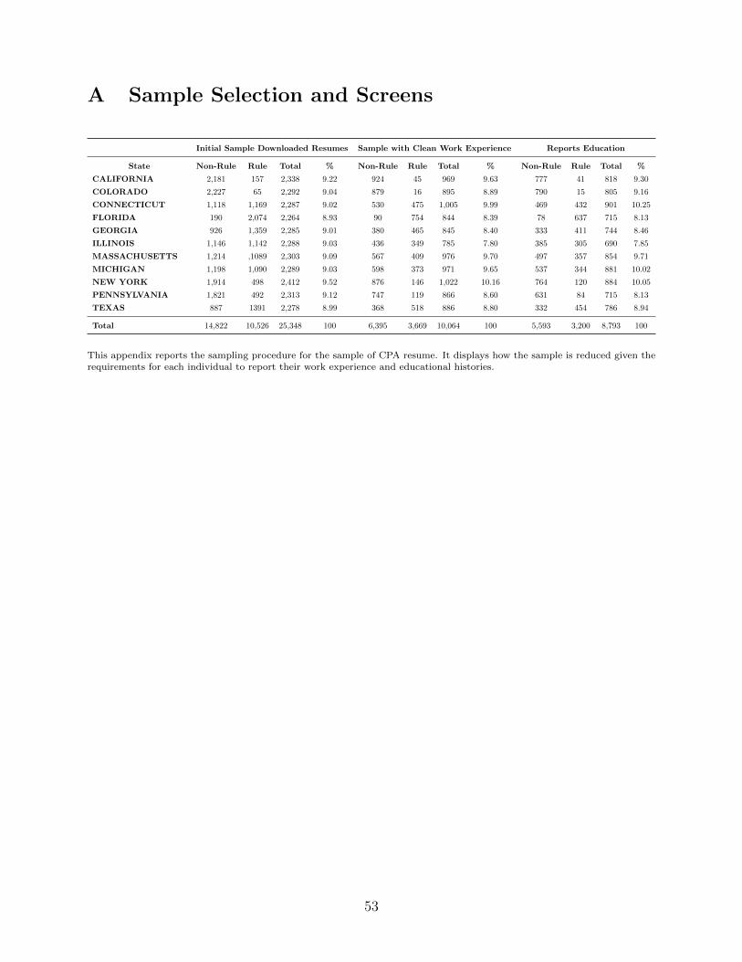
A Sample Selection and Screens

Initial Sample Downloaded Resumes Sample with Clean Work Experience Reports Education

State Non-Rule Rule Total % Non-Rule Rule Total % Non-Rule Rule Total %

CALIFORNIA 2,181 157 2,338 9.22 924 45 969 9.63 777 41 818 9.30

COLORADO 2,227 65 2,292 9.04 879 16 895 8.89 790 15 805 9.16

CONNECTICUT 1,118 1,169 2,287 9.02 530 475 1,005 9.99 469 432 901 10.25

FLORIDA 190 2,074 2,264 8.93 90 754 844 8.39 78 637 715 8.13

GEORGIA 926 1,359 2,285 9.01 380 465 845 8.40 333 411 744 8.46

ILLINOIS 1,146 1,142 2,288 9.03 436 349 785 7.80 385 305 690 7.85

MASSACHUSETTS 1,214 ,1089 2,303 9.09 567 409 976 9.70 497 357 854 9.71

MICHIGAN 1,198 1,090 2,289 9.03 598 373 971 9.65 537 344 881 10.02

NEW YORK 1,914 498 2,412 9.52 876 146 1,022 10.16 764 120 884 10.05

PENNSYLVANIA 1,821 492 2,313 9.12 747 119 866 8.60 631 84 715 8.13

TEXAS 887 1391 2,278 8.99 368 518 886 8.80 332 454 786 8.94

Total 14,822 10,526 25,348 100 6,395 3,669 10,064 100 5,593 3,200 8,793 100

This appendix reports the sampling procedure for the sample of CPA resume. It displays how the sample is reduced given therequirements for each individual to report their work experience and educational histories.

53

B Seniority Position Classification Scheme

Panel A: List of Titles included in Each Seniority Level

Level-1: Low Seniority % Level-2: Medium Seniority % Level-3: High Seniority %

Staff Accountant 11.35 Senior Accountant 3.49 Controller 11.95

Associate 3.66 Senior Auditor 2.38 Chief Financial Officer 6.36

Audit Associate 3.27 Manager 2.20 CFO 4.57

Auditor 3.26 Tax Manager 2.02 Assistant Controller 3.13

Accountant 3.17 Senior Associate 1.80 Corporate Controller 2.65

Tax Associate 2.68 Audit Manager 1.79 Partner 2.12

Internal Auditor 2.28 Senior Manager 1.75 President 1.93

Staff Auditor 2.10 Accounting Manager 1.70 Owner 1.67

Assurance Associate 1.85 Consultant 1.56 Vice President 1.48

Administrative Staff 1.61 Audit Senior 1.24 Financial Controller 0.88

Bookkeeper 1.15 Financial Analyst 1.10 VP Finance 0.62

Accounting Assistant 1.02 Director 0.99 Vice President of Finance 0.52

Tax Accountant 1.02 Senior Financial Analyst 0.95 Assistant Corporate Controller 0.49

Audit Staff 0.62 Director of Finance 0.82 CEO 0.47

Accounting Clerk 0.60 Finance Manager 0.76 Managing Partner 0.45

Panel B: Descriptives

Full Sample

Obs Mean Median Std. DeviationLow Seniority Time to Promotion 7,167 3.058 0.833 6.270

Job Order 7,167 2.252 2.000 1.776Medium Seniority Time to Promotion 23,493 9.061 6.583 9.347

Job Order 23,493 3.965 3.000 2.673High Seniority Time to Promotion 10,995 15.533 13.750 12.117

Job Order 10,995 5.206 5.000 2.916

This appendix provides examples of job titles that have been classified as belonging to one of the three seniority groups. Highseniority positions contain jobs titles that make reference to top-level corporate officers in corporations or partners in publicaccounting firms. The medium seniority group contains job titles that refer to middle-management positions as well as seniorpositions at firms. Finally, the low seniority group contains job titles of entry-level positions at the firm. Panel A providesexamples of titles that have been classified into each of the seniority levels. Panel B provides descriptive statistics on the averagerank order position of titles in individuals careers as well as the average time spent in each level (for the high seniority it is thetime individuals take to get to these positions).

54

C Duration Analysis: Promotions(Matched Sample)

Panel A: Percentage of Individuals yet to be Promoted

This panel displays the two Kaplan–Meier Survival estimates for promotion to level-two and level-three seniority positions. Thepercentage of the cohort that remains in the initial level-one seniority position is graphed on the y-axis, while the number ofyears elapsed is graphed on the x-axis. The figure on the left is for promotions from level one to level two while the one on theright is for promotions to level-three seniority positions. The solid blue line plots the estimate for the Rule cohort while thedashed line plots the estimate for their non-Rule counterparts.

Panel B: Cox Proportional Hazard Model for the Effect of the Rule on time till Pro-motion

Level-2 Seniority Promotions Level 3 Seniority Promotions

Rule 1.051 1.035 1.032 1.034 0.971 0.967 0.947 1.018(1.41) (0.96) (0.87) (1.49) (-0.56) (-0.63) (-1.04) (0.16)

Male 1.173*** 1.285*** 1.206*** 0.805*** 0.834*** 0.892*(4.37) (6.75) (4.99) (-4.02) (-3.35) (-2.00)

Cohort Fixed Effects No No No No No No No NoState Fixed Effects No No No Yes No No No YesLR Chi2 1.98 21.25*** 321.87*** 305.47*** 0.31 16.20*** 204.60*** 155.02***N 3209 3209 3209 3209 1467 1467 1467 1467

This panel reports the Cox proportional hazard model for the effect of the Rule on the time till promotion from level-one tolevel-two and level-three seniority positions on a matched sample based on age and gender. I control for gender in Models 2and 3. Model 4 includes state fixed effects. The coefficients are exponentiated for ease of interpretation and Z statistics arereported in parentheses. Significance levels are indicated by: * p < 0.10, ** p < 0.05, *** p < 0.01.

55