Working Paper 44July 2004 (Revised 9-6-11)

Counting Chickens When They Hatch: Timing and the Effects of Aid on Growth

Abstract

Recent research yields widely divergent estimates of the cross-country relationship between foreign aid receipts and economic growth. We propose and test two reasons for this divergence, both of which relate to the timing of effects between aid and growth. First, these studies have insufficiently considered the lag with which aid might affect growth, particularly certain kinds of aid. Second, they have sought to reduce the bias from contemporaneous reverse causation with the use of instrumental variables that appear to be invalid, weak, or both. We reanalyze data from the three most influential published aid-growth studies, strictly conserving their regression specifications, adding sensible assumptions about timing and avoiding questionable instruments. With these changes, the research designs from all of these studies yield one finding: that increases in aid have been followed on average by modest increases in investment and growth. The most plausible explanation is that aid causes some degree of growth in recipient countries, though the magnitude of this relationship is modest, varies greatly across recipients, and diminishes at high levels of aid.

JEL Codes: F35, O11, O19

www.cgdev.org

Michael A. Clemens, Steven Radelet, Rikhil R. Bhavnani, and Samuel Bazzi

Counting Chickens When They Hatch:Timing and the Effects of Aid on Growth

Michael ClemensCenter for Global Development

Steven RadeletUSAID

Rikhil R. BhavnaniUniv. of Wisconsin–Madison

Samuel BazziUniversity of California–San Diego

Michael Clemens et al. 2004. “Counting Chickens When They Hatch: Timing and the Effects of Aid on Growth.” CGD Working Paper 44. Revised September 6, 2011. Washington, D.C.: Center for Global Development. http://www.cgdev.org/content/publications/detail/2744

Center for Global Development1800 Massachusetts Ave., NW

Washington, DC 20036

202.416.4000(f ) 202.416.4050

www.cgdev.org

The Center for Global Development is an independent, nonprofit policy research organization dedicated to reducing global poverty and inequality and to making globalization work for the poor. Use and dissemination of this Working Paper is encouraged; however, reproduced copies may not be used for commercial purposes. Further usage is permitted under the terms of the Creative Commons License.

The views expressed in CGD Working Papers are those of the authors and should not be attributed to the board of directors or funders of the Center for Global Development.

Counting chickens when they hatch:Timing and the effects of aid on growth

Michael A. Clemens∗

Center for Global DevelopmentSteven Radelet

U.S.A.I.D.

Rikhil R. BhavnaniUniv. of Wisconsin, Madison

Samuel BazziUniv. of California, San Diego

September 6, 2011

Forthcoming in Economic Journal

Abstract: Recent research yields widely divergent estimates of the cross-country relationshipbetween foreign aid receipts and economic growth. We propose and test two reasons for thisdivergence, both of which relate to the timing of effects between aid and growth. First, thesestudies have insufficiently considered the lag with which aid might affect growth, particularlycertain kinds of aid. Second, they have sought to reduce the bias from contemporaneousreverse causation with the use of instrumental variables that appear to be invalid, weak,or both. We reanalyze data from the three most influential published aid-growth studies,strictly conserving their regression specifications, adding sensible assumptions about timingand avoiding questionable instruments. With these changes, the research designs from all ofthese studies yield one finding: that increases in aid have been followed on average by modestincreases in investment and growth. The most plausible explanation is that aid causes somedegree of growth in recipient countries, though the magnitude of this relationship is modest,varies greatly across recipients, and diminishes at high levels of aid.

JEL Classification Numbers: F35, O11, O19.

∗We benefited greatly from extensive discussions with William Easterly, Aart Kraay, Simon Johnson,David Roodman, and Arvind Subramanian. We appreciate numerous substantive suggestions from MartinAlsop, Nancy Birdsall, Francois Bourguignon, William Cline, Paul Collier, Shanta Devarajan, Alan Gelb,Stephen Knack, Daniel Morrow, Peter Timmer, Nicholas Stern, Mark Sundberg, Jeremy Weinstein, AdrianWood, four anonymous referees, and seminar participants at the Center for Global Development (CGD),the World Bank, the International Monetary Fund, American University, the U.S. Treasury, the UK Depart-ment for International Development, and the U.S. Agency for International Development. We are gratefulfor the assistance of Valérie Gaveau and Virginia Braunstein of the OECD. This research was generouslysupported by the William and Flora Hewlett Foundation and CGD. All viewpoints and any errors are thesole responsibility of the authors and do not represent CGD, its Board of Directors, or its funders.

1 Introduction

Economists have spent decades debating, without resolution, the cross-country relationship

between foreign aid receipts and economic growth. Some find that aid robustly causes positive

economic growth on average. Others cannot distinguish the average effect from zero. Still

others find an effect only in certain countries, such as those with good policies or governance.

Wearied readers of this literature would be right to wonder what produces diverse findings

from apparently the same aid and growth data.

Here we show that two traits of previous research help explain why different studies

reach different conclusions. Both traits relate to how these studies treat the timing of causal

relationships between aid and growth. First, the most cited research has focused on measuring

the effect of aggregate aid on contemporaneous growth, while many aid-funded projects can

take a long time to influence growth. Funding for a new road might affect economic activity

in short order, funding for a vaccination campaign might only affect growth decades later,

and humanitarian assistance may never affect growth. Second, because current growth is

likely to affect current aid, these studies require a strategy to disentangle correlation from

causation. They have tended to rely on instrumental variables, but the instruments that have

been used are of questionable validity and strength. When these issues are addressed, the

divergence in empirical findings is greatly reduced.

We show this by stepwise altering the research design of the three most influential papers

in the aid and growth literature. We hold all else constant: We begin by reconstructing their

data and using precisely their regression specifications. This transparency and consistency

is essential in a literature that has been alternately described as marred by aid proponents’

“confirmation bias” (Easterly 2006, 48) or described as marred by aid opponents’ selective

reading of the empirical evidence (Hansen and Tarp 2000, 393). We avoid poor-quality in-

strumental variables and instead address potential biases from reverse and simultaneous

causation by the more transparent methods of lagging and differencing. We test only one

1

lag structure (the simplest) and only one disaggregation of aid, both of which were estab-

lished before running the regressions and were not altered thereafter. All other aspects of

the regressions remain as in the authors’ original papers.

This exercise reveals that the results of all three studies change markedly 1) when we allow

aid to affect growth with a time lag, 2) when first-differencing removes the effects of time-

invariant omitted variables, and 3) when we consider only those portions of aid that could

be intended or expected to produce growth within a few years. These steps allow us to avoid

the use of poor-quality instrumental variables that have pervaded this literature. With these

sensible alterations, the data reveal that over the last three decades, substantial increases in

aid receipts were followed on average by small increases in investment and growth.

The fact that some amount of growth typically follows aid receipts does not per se

establish causation. We discuss and test other possible explanations, but all are less plausible

than aid causing some nonzero amount of growth. The results are not an artifact of dynamic

panel bias, of our assumed functional form, or of mean reversion in the data. The magnitudes

of the coefficients we estimate are reasonable and consistent across different specifications,

with a one percentage-point increase in aid/GDP (at mean aid levels) typically being followed

within several years by modest increases in investment and growth: a 0.3–0.5 percentage-

point increase in investment/GDP and a 0.1–0.2 percentage-point increase in growth of real

GDP per capita.

These results do not in any way suggest that aid always “works” or that large amounts of

aid can be the central pillar of any given country’s growth strategy. The results do suggest

that the effect of aid on growth is positive on average across all countries, but is limited

and quite modest in comparison with other determinants of growth, and is negative in some

countries. We begin by putting these findings in broader context.

2

2 Four decades of diverse findings

Griffin and Enos (1970) launch this literature by reporting zero or negative bivariate cor-

relation between aid receipts and growth in 27 countries, a finding essentially echoed by

Weisskopf (1972). Papanek (1972, 1973) is the first to conduct a multivariate regression of

growth on aid, in a model resembling

˙yi,t/yi,t = α + βdneti,t +Xi,tη + εi,t (1)

where yi,t is income per capita in country i at time t, dneti,t is net disbursements of aid, Xi,t

is a vector of country characteristics, α and β are constants, η is a vector of constants, εi,t

is white noise, and a superscript dot represents the derivative with respect to time. He and

Gulati (1978) find a significant positive partial correlation between aid and growth in 51

countries during 1950-1965, but not in the Americas.

Over (1975) and Mosley (1980) first attempt to isolate the causal portion of the aid-

growth relationship with instrumental variables, in models resembling

˙yi,t/yi,t = α + βdneti,t +Xi,tη + εi,t

dneti,t = Zi,tζ + νi,t

(2)

where Zi,t is a vector of exogenous instruments, ζ is a vector of constants, and νi,t is white

noise. Several related studies follow, each using different countries, years, and instruments.

All are troubled by relatively short time periods and limited country samples (Gupta and

Islam 1983; Mosley et al. 1987; Levy 1988).

Boone (1996) ushers in the current wave of aid-growth studies with more complete data

than any predecessor. Across 96 countries, between 1971 and 1990, he finds no relationship

between aid receipts and investment. He concludes that “aid programs have not ... engendered

or correlated with the basic ingredients that cause ... growth.” He bases this conclusion on

3

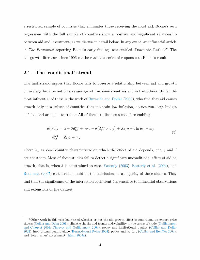
a restricted sample of countries that eliminates those receiving the most aid; Boone’s own

regressions with the full sample of countries show a positive and significant relationship

between aid and investment, as we discuss in detail below. In any event, an influential article

in The Economist reporting Boone’s early findings was entitled “Down the Rathole”. The

aid-growth literature since 1996 can be read as a series of responses to Boone’s result.

2.1 The ‘conditional’ strand

The first strand argues that Boone fails to observe a relationship between aid and growth

on average because aid only causes growth in some countries and not in others. By far the

most influential of these is the work of Burnside and Dollar (2000), who find that aid causes

growth only in a subset of countries that maintain low inflation, do not run large budget

deficits, and are open to trade.1 All of these studies use a model resembling

˙yi,t/yi,t = α + βdneti,t + γqi,t + δ(dneti,t × qi,t

)+Xi,tη + θ ln yi,t + εi,t

dneti,t = Zi,tζ + νi,t

(3)

where qi,t is some country characteristic on which the effect of aid depends, and γ and δ

are constants. Most of these studies fail to detect a significant unconditional effect of aid on

growth, that is, when δ is constrained to zero. Easterly (2003), Easterly et al. (2004), and

Roodman (2007) cast serious doubt on the conclusions of a majority of these studies. They

find that the significance of the interaction coefficient δ is sensitive to influential observations

and extensions of the dataset.

1Other work in this vein has tested whether or not the aid-growth effect is conditional on export priceshocks (Collier and Dehn 2001); climatic shocks and trends and volatility in the terms of trade (Guillaumontand Chauvet 2001; Chauvet and Guillaumont 2004); policy and institutional quality (Collier and Dollar2002); institutional quality alone (Burnside and Dollar 2004); policy and warfare (Collier and Hoeffler 2004);and ‘totalitarian’ government (Islam 2003a).

4

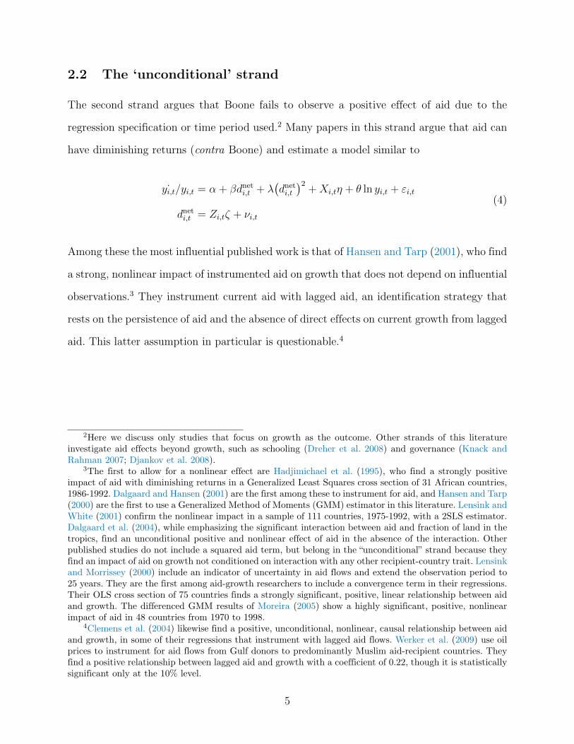
2.2 The ‘unconditional’ strand

The second strand argues that Boone fails to observe a positive effect of aid due to the

regression specification or time period used.2 Many papers in this strand argue that aid can

have diminishing returns (contra Boone) and estimate a model similar to

˙yi,t/yi,t = α + βdneti,t + λ(dneti,t

)2+Xi,tη + θ ln yi,t + εi,t

dneti,t = Zi,tζ + νi,t

(4)

Among these the most influential published work is that of Hansen and Tarp (2001), who find

a strong, nonlinear impact of instrumented aid on growth that does not depend on influential

observations.3 They instrument current aid with lagged aid, an identification strategy that

rests on the persistence of aid and the absence of direct effects on current growth from lagged

aid. This latter assumption in particular is questionable.4

2Here we discuss only studies that focus on growth as the outcome. Other strands of this literatureinvestigate aid effects beyond growth, such as schooling (Dreher et al. 2008) and governance (Knack andRahman 2007; Djankov et al. 2008).

3The first to allow for a nonlinear effect are Hadjimichael et al. (1995), who find a strongly positiveimpact of aid with diminishing returns in a Generalized Least Squares cross section of 31 African countries,1986-1992. Dalgaard and Hansen (2001) are the first among these to instrument for aid, and Hansen and Tarp(2000) are the first to use a Generalized Method of Moments (GMM) estimator in this literature. Lensink andWhite (2001) confirm the nonlinear impact in a sample of 111 countries, 1975-1992, with a 2SLS estimator.Dalgaard et al. (2004), while emphasizing the significant interaction between aid and fraction of land in thetropics, find an unconditional positive and nonlinear effect of aid in the absence of the interaction. Otherpublished studies do not include a squared aid term, but belong in the “unconditional” strand because theyfind an impact of aid on growth not conditioned on interaction with any other recipient-country trait. Lensinkand Morrissey (2000) include an indicator of uncertainty in aid flows and extend the observation period to25 years. They are the first among aid-growth researchers to include a convergence term in their regressions.Their OLS cross section of 75 countries finds a strongly significant, positive, linear relationship between aidand growth. The differenced GMM results of Moreira (2005) show a highly significant, positive, nonlinearimpact of aid in 48 countries from 1970 to 1998.

4Clemens et al. (2004) likewise find a positive, unconditional, nonlinear, causal relationship between aidand growth, in some of their regressions that instrument with lagged aid flows. Werker et al. (2009) use oilprices to instrument for aid flows from Gulf donors to predominantly Muslim aid-recipient countries. Theyfind a positive relationship between lagged aid and growth with a coefficient of 0.22, though it is statisticallysignificant only at the 10% level.

5

2.3 The ‘null’ strand

A third strand argues that the evidence gathered since 1990 simply confirms Boone’s null

result. They expand on Boone by using growth directly as the dependent variable rather

than investment, and by using more extensive data. By far the most influential of these

is the work of Rajan and Subramanian (2008), whose core results instrument for aid with

measures of country size and political ties to donors, much as Boone did. On this null result

they base the policy conclusion that “the aid apparatus will have to be rethought.” Below

we dissect this and the other most influential studies in this literature.

3 A way forward: Timing and identification

In this paper we explore the reasons for the divergence among these strands of literature.

We find that when straightforward changes are made to the most influential papers in each

strand, much of the divergence disappears. These are 1) allowing aid to affect growth with

a time lag, 2) first-differencing to eliminate omitted variable bias from time-invariant unob-

served traits, and 3) considering only those portions of aid that might produce growth within

a few years. This allows us to avoid the use of potentially invalid and weak instrumental

variables and seeking causal identification by more transparent means. Here we discuss the

reasons for these choices.

3.1 The timing of aid effects

Clemens et al. (2004) argue that Boone and his successors may have failed to observe a

positive effect of aggregate aid because some aid is aimed at activities whose growth impact

has slim theoretical basis within the time periods used in the panel. These include flows that

are not intended or used to promote expansion in generalized productive capacity (such as

humanitarian assistance or disaster relief) as well as flows whose effect on overall national

growth, if it ever arrives, might come long after the time period under study (such as a

6

vaccination campaign or school feeding project).5

The question of when to test for growth impacts plagues the entire growth literature, not

just aid-growth research. Empirical research on the determinants of growth cannot escape

the selection of a fixed observation period, but “selecting the time intervals over which to

study growth ... is a question that remains largely unsettled” (Temple 1999, 132). Lengthy

observation periods make it possible to capture long-term growth consequences of changes

in country traits, but require cross-section estimators plagued by limited degrees of freedom,

reverse causation, and simultaneity bias from omitted variables.

Short periods decrease the bias from omitted variables that change slowly over time, and

permit estimators with country effects (Islam 1995) to entirely remove the bias of omitted

time-invariant traits. But the shorter the periods, the more “the model likely misspecifies

the timing between growth and its determinants” and comes to be “dominated by measure-

ment error” (Barro 1997, 42 and 15). Nevertheless, “[t]oo often researchers use fixed effects

approaches to analyze the effects of variables ... that will affect growth only with a long lag”

(Temple 1999, 132). Hypothesis tests regarding these growth determinants will suffer from

low power. No consensus solution to this dilemma has emerged. Durlauf and Quah (1999)

warn against short periods, while Islam (2003b, 332) agrees with Temple (1999, 113) that

“the use of panels is often the best way forward”.

Our approach is as follows: 1) We use short-period panel data, which allow country fixed-

effects to be differenced away; 2) we allow for the possibility that the growth effect of aid

arrives with a time lag; and 3) consider a subset of aid that does not include aid flows whose

growth effect is most likely to arrive decades in the future, or never.

5Other studies before Clemens et al. (2004) consider aid disaggregated by purpose, but none with the aimof analyzing the growth impact within an appropriate time horizon. Owens and Hoddinott (1999) find thathousehold welfare in Zimbabwe is increased by development aid (such as agricultural extension) more than byhumanitarian aid (such as food aid), even in humanitarian emergencies. Mavrotas (2002) disaggregates aidinto “program,” “project,” and “technical assistance” flows, and finds a negative correlation between growthand all three types of aid in India 1970-92.

7

3.2 A lack of reliable instruments

All of the major studies of aid and growth since Boone’s have used instrumental variables

for aid. Certainly it is important to employ some strategy for identifying the causal compo-

nent of the aid-growth relationship, since any observed correlation between aid and growth

could plausibly result from reverse causation or simultaneous causation by omitted variables.

The use of instrumental variables is only one approach to identification, however, and this

literature’s search for strong, valid instrumental variables has encountered difficulties.

Here we discuss the instruments used in the most influential published studies in this

literature.6 Three of these, whose regression specifications we recreate below, are Boone,

Burnside and Dollar (“BD”), and Rajan and Subramanian (“RS”). We also discuss the in-

struments used in a fourth published study as influential as these others, Hansen and Tarp

(“HT”), and those in Clemens et al. (“CRB”), both of which use regression specifications

similar to those in BD. All of these studies use as instruments some measure of political ties

to donors (former colonial relationships, arms sales, and so on). The remaining instruments

are primarily either related to lagged aid flows (HT, CRB) or to the size of the recipient

country (Boone, BD, RS).

All of these instruments raise questions about how strong or valid we can take them to be.

Lagged aid flows might well affect current growth, biasing the resulting coefficient on aid. HT

and CRB find positive and statistically significant effects of aid on growth. But while both

HT and CRB test for correlation between the instruments and the residuals, existing tests of

this correlation have notoriously low power to reject the null of no correlation. Instrumenting

for current aid with lagged aid raises the possibility that the coefficient on aid is substantially

biased by invalid instruments.

6We measure influence by citations of all versions of each study in the Google Scholar internet searchengine as of July 22, 2010, divided by the number of years since (and including) the year of publication.The four most influential studies are Burnside and Dollar (198 citations/year, 2,176 total), Rajan andSubramanian (125 citations/year, 377 total), Hansen and Tarp (60 citations/year, 597 total), and Boone (49citations/year, 741 total).

8

We come now to the core regressions of Boone, BD, and RS, all of which instrument for

aid primarily with some combination of political ties to donors and the size of the recipient

country’s population.7 In all three studies, population size is responsible for most of the

instrumentation power.

In the core results of Boone and RS, in fact, essentially all instrument strength derives

from population size alone. There are two ways to see this. First, the single constructed

instrument used in the core regressions of RS is almost perfectly correlated with population

size. The absolute value of the correlation between the RS instrument and ln(population)

is 0.93 in their 1970-2000 period and 0.95 in the 1980-2000 and 1990-2000 periods (Bazzi

and Clemens 2010). The three-stage RS procedure constructs an instrument that contains

almost no information beyond the size of the recipient’s population, and does not materially

improve on simply instrumenting with population size.

Second, and more directly, when the instruments containing population are included

in the second stage regression, instrumentation power drops dramatically in Boone, BD,

and RS. In Boone and RS, it collapses completely. Table 1 shows this result.8 The first

column shows a core result of Boone’s with aid instrumented by population size and several

variables capturing political ties. The Cragg and Donald (1993) and Kleibergen and Paap

7The excluded instruments in the core specification of Boone are ln(population), dummy for ‘friend’ of USand dummy for ‘friend’ of OPEC (where ‘friend’ equals one if the recipient receives more than 1% of the totalaid budget of each donor), and dummy for ‘friend’ of France (defined as membership in the Franc zone). Theexcluded instruments in BD are ln(population), lagged arms imports/total imports, Egypt dummy, Franczone dummy, Central America dummy, ln(initial income) × policy, ln(population) × policy, (lagged armsimports/total imports) × policy,

(ln(initial income

)2) × policy, and(ln(population

)2) × policy (where“policy” is an index of inflation, budget balance, and openness to trade). The excluded instrument in RSis a single recipient-level variable constructed from donor-recipient measures of the following instruments:dummies for common language, dummies for current and former colonial relationships, separate dummiesfor former colonies of four countries (UK, France, Spain, and Portugal), the logarithm of the ratio of donorpopulation to recipient population, and the interaction of the preceding variable with a dummy for currentor past colonial relationship.

8The regressions of Table 1 use the original datasets of BD and RS. The original dataset used byBoone no longer exists (personal communication from the author). We meticulously reconstructed a datasetto mimic Boone’s, using his sources and variable definitions. Regressions identical to Boone’s publishedregressions using this reconstructed dataset give coefficient estimates corresponding very closely to Boone’s.Our reconstruction of Boone’s data is available upon request and is described in the appendix.

9

(2006) F -statistics are well over 4, roughly the critical value for strong instrumentation as

defined by Stock and Yogo (2005).9 The second column shows the same regression with

ln(population) included in the second stage; instrumentation strength collapses. This means

that the remaining instruments do not capture a sufficient degree of variance in aid flows to

meaningfully remedy the bias of simply running the regression with OLS.

The next three columns of Table 1 show that the BD instrumentation strategy also relies

heavily, but not completely, on population for its strength. When all three BD instruments

containing population size are included in the second stage, the Cragg-Donald statistic falls

from about 20 to about 7. The next column includes all ‘policy’ related variables in the

second stage, since current growth could easily affect current budget balance or inflation,

which would invalidate policy as an instrument. With these in the second stage as well,

instrumentation becomes weak.

The remainder of Table 1 shows that when ln(population) is included in the second stage

of Rajan and Subramanian’s core cross-section regressions, using the authors’ original data,

instrumentation strength is gone. The Cragg-Donald statistic falls from about 32 to about

0.1. Rajan and Subramanian’s other, more plausibly valid “political” instrumental variables

therefore do not capture enough variance in aid for their validity to be relevant. The results

in Table 1 collectively mean that Boone and RS are effectively instrumenting for aid with

population size alone, and BD are resting their instrumentation strength primarily upon

population size.10

Relying on country population as an instrument throws into serious doubt the validity of

the entire instrumentation strategy, and therefore of all regression results. There are several

9Stock and Yogo (2005) show that a Cragg-Donald F -statistic over 4 is likely to signify instrumentationof sufficient strength that bias in the second-stage coefficient from weak instrumentation is less than 30% ofthe OLS bias. Kleibergen and Paap (2006) present a related F-statistic that is robust to heteroskedasticity.The Kleibergen-Paap statistic does not yet have a corresponding set of critical values, but values well belowthe Cragg-Donald critical values suggest that further investigation is essential.

10In the Rajan and Subramanian regressions that allow for a nonlinear effect of aid, instrumentation isweak even when population is not included in the second stage (Bazzi and Clemens 2010).

10

channels omitted from the second stages of all of these regressions through which population

size has been found to directly affect growth in published research. Any one such channel

would invalidate population as an instrument in these aid-growth regressions. These channels

include the extent of internal and external trade (Frankel and Romer 1999), the mix of goods

that a country exports (Hausmann et al. 2007), and the extent of political integration with

neighbors (Spolaore and Wacziarg 2005), among others. In all of the above studies and others,

population is a strong instrument for a variable that has been found to directly affect growth

that is not included in any aid-growth regression. This throws strong doubt on the ability of

the Boone and RS studies to test the hypotheses they seek to test.11

As a robustness check, RS later employ an alternative identification strategy. They use

the Generalized Method of Moments (GMM) with panel data to instrument for current

aid levels with lagged differences in aid and other regressors, and to instrument for current

differences in aid with lagged levels of aid and other regressors. It is theoretically possible

that such instruments could strongly instrument for current levels or differences in aid,

but in the RS dataset they do not. Existing panel and system GMM estimators do not

provide a clear way to test for weak instruments, but when analogous regressions are run

using Two-Stage Least Squares, instrumentation both by lagged levels and lagged differences

of the RS regressors is extremely weak, with Cragg-Donald F-statistics far below critical

values for strong instruments (Bazzi and Clemens 2010). This is more serious than the

aforementioned possible invalidity of lagged aid as an instrument, which is also a concern

here; weak instrumentation means that the coefficient estimates in RS can be as plagued

with bias as simple OLS estimates (Stock and Yogo 2005).

Many authors have searched energetically for an instrumental variable for aid that is

strong and does not raise important questions about its validity. This review nevertheless

suggests that readers of the most influential published aid-growth studies should not discard

11It also casts doubt on the BD results, though not as clearly, since BD’s instruments remain marginallystrong by the standard of Stock and Yogo even when population is no longer an excluded instrument.

11

all doubts that such an instrument has been found.

4 Method: An alternative approach to identification

Lacking an instrumental variable that we can confidently consider both strong and valid, how

might causal identification proceed? We apply the following three-step method to the three

most influential regression specifications in the aid-growth literature. These steps eliminate

most of the major channels through which anything besides causation of growth by aid could

generate a positive correlation between growth and aid.

We first re-run the core regressions in each of the studies in order to replicate their results.

Holding the regression specification constant, we then lag the aid variable, and difference

the results. This step controls for country fixed effects, allows for aid to have an impact on

growth in the subsequent time period, and allows us to avoid relying on a potentially weak

or invalid instrument to identify the impact of foreign aid on growth. Next, we explore the

effects of restricting the aid variable to only those portions of aid that might be expected

to affect growth within the relevant time horizon. We call this restricted aid variable “early

impact” aid. Finally, we extend the time horizon for the regressions to all years of currently

available data, following Easterly et al. (2004).12

4.1 Reconstructing data used by previous studies

Our method raises a series of technical challenges. First among these is the challenge of

faithfully reconstructing the datasets used in previous studies. For the BD and RS studies

this is easy; the authors have graciously made their original datasets available. The Boone

analysis required more effort because the original Boone dataset no longer exists. Boone’s

sources and variable definitions are sufficiently clear, however, to allow us to reconstruct

12Because BD and HT use essentially the same data and periods, we treat them as a unit. The resultsbelow, then, are divided in three parts, exploring in turn the results of Boone, BD (and HT), and RS.

12

his dataset from publicly available sources. Regressions on our reconstructed dataset give

coefficient estimates closely reflecting those in Boone’s paper, so we feel comfortable asserting

that in all three cases we are working with data that are either identical to or extremely

similar to the data used by the original authors.13

4.2 Disaggregating aid

A second challenge is to restrict the aid variable to “early-impact” aid, which excludes those

portions of aid that might not be expected to cause growth during the time period under

study. If there is any ambiguity about what is being funded—notably in the case of budget-

support aid—we leave it in “early impact” aid, since some or all of it could be spent on

activities that might be expected to affect growth within a few years. The inclusion of aid

that would not have such an effect would bias the coefficient on aid towards zero.

“Early impact” aid includes 1) budget support or “program” aid given for any purpose,

and 2) project aid given for real sector investments for infrastructure or to directly support

production in transportation (including roads), communications, energy, banking, agriculture

and industry. It excludes any aid flow that clearly and primarily funds an activity whose

growth effect might arrive far in the future or not at all, such as 1) all technical cooperation,

2) most social sector investments, including in education, health, population control, and

water, 3) all humanitarian aid such as emergency assistance during natural disasters and

food aid, and 4) donors’ administrative/overhead costs and expenditures on “promotion of

development awareness”.14

4.3 Estimating ‘early impact’ aid

A third challenge is that for most donors in most years covered by the studies we investigate,

the OECD reports purpose-disaggregated aid commitments but only aggregate disburse-

13The appendix compares our data with the published results from each paper.14The appendix describes in detail the definition of “early-impact” aid.

13

ments. Most donors began reporting purpose-disaggregated commitments to the OECD in

the early 1970s, but OECD data on purpose-disaggregated aid disbursements only begin for

a subset of donors in 1990, and do not embrace all donors until 2002.

One approach to this problem is to use information contained in the historical purpose-

disaggregated commitments to estimate purpose-disaggregated disbursements. We illustrate

this method by example. To estimate “early impact” disbursements to Ghana in 1983, we

begin with early-impact commitments from the United Kingdom to Ghana in 1983 and

divide by total UK commitments to Ghana in 1983. The resulting ratio is multiplied by

total UK disbursements to Ghana in the same year, resulting in a dollar estimate of “early

impact” disbursements from UK to Ghana in 1983. The same procedure is repeated for each

of Ghana’s donors to achieve a separate estimate for each donor, and finally these amounts

are summed across donors to yield an estimate of the total dollar amount of “early impact”

aid disbursed to Ghana in 1983 by all donors. This sum is then divided by the size of the

Ghanaian economy in that year. This same procedure yields our base estimate of “early

impact” aid disbursements for each recipient-year.15

This method is theoretically attractive because it is reasonable that the share of aid dis-

bursed for a broad category of purposes generally reflect the share of aid committed for that

broad category of purposes. It is not easy to posit a model of donor behavior that would lead

donors who commit their aid mostly for roads—consistently over several years—to then con-

sistently disburse aid mostly for schools, or vice versa. It is furthermore empirically attractive

15The numerator for early impact aid is the product of gross ODA (Net ODA + Repayments) fromOECD DAC Table 2 and the ratio of total early impact ODA commitments as classified in the appendixover total ODA commitments from the OECD CRS. This product is calculated by donor-recipient pair andthen summed across all donors for a given recipient-year. The denominator in BD and RS is GDP in currentUSD and in Boone is GNI in current US dollars. When we include “early impact” aid in any regression, it isaccompanied by a term for repayments on aid. This is because by definition, any flow of aid disaggregatedby purpose is a gross flow, not a net flow, since repayments on aid are not separated by purpose. Grossrepayments on aid must therefore be included as a covariate in any regression that disaggregates aid ifthe regression results are to be comparable to other regressions whose regressor is net aid (that is, netof repayments). When the aid variable is net aid then repayments can affect growth, so a fundamentallydifferent regression is being run if the aid variable is a gross flow and repayments are excluded. This wouldnot be true if there were a theoretical reason to believe that repayments on aid cannot affect growth; we seeno such reason.

14

because in the few years where true purpose-disaggregated disbursements are available for

comparison (2002-2006), the estimated fraction of disbursements in each category is strongly

correlated with the true fraction. In this period, the correlation between our estimate of

“early impact” disbursements as a fraction of total disbursements and true “early impact”

disbursements as a fraction of total disbursements is 0.74.

4.4 True causation versus Granger causation

What remains after these corrections is a measurement that, while it does not meet the strict

scientific definition of causation that would arise from a randomized experiment, does answer

a question of great policy relevance: Are aid receipts followed within several years by any

degree of increase in economic growth? That is, does aid exhibit Granger (1969) causation of

growth? Certainly a donor interested in promoting economic growth in the recipient would

want to know the answer.

It is naturally possible for non-causal mechanisms to produce Granger causality. It is

possible, for example, that aid donors correctly foresee recipients’ growth patterns several

years into the future. But evidence suggests that growth several years into the future is

highly unpredictable (Easterly et al. 1993) and that donors make large errors in forecasting

recipients’ growth even in the short term (Batista and Zalduendo 2004). This pathway is very

doubtful. It is also possible that this pattern could arise as an artifact of mean reversion in

growth combined with causation of aid by growth. That is, poor growth performance at time

t could be both 1) typically accompanied by more aid at time t and 2) typically followed by

better growth performance at time t+1, which would produce a correlation between current

aid and later growth, as Roodman (2008) conjectures. This is easily tested.

15

5 Results

The results of the most influential aid-growth regressions in the literature would be different

and remarkably uniform if two things had been different about them: first, if they had allowed

aid to affect growth with a time lag and removed aid unlikely to affect growth within that

window, and second, if they had used an identification strategy that does not rely on poor

instrumental variables. Here we demonstrate this using faithful reconstructions of the data

and regression specifications used in Boone, BD, and RS. Table 3 presents summary statistics

for key variables from the three databases.

5.1 The Boone specification

Table 4 explores the effect of piecewise changes to the regressions of Boone (1996). Columns 1

and 2 show no relationship between aid and investment in Boone’s OLS and 2SLS regressions,

holding the sample constant (following Boone’s Table 5, column 2 and Boone’s Table 4,

column 4, row 3). However, these regressions use Boone’s “base” sample of countries, which

deletes from the sample all countries that received more than 15% of GNI in aid. He does

this “because it appears that beyond these levels aid is no longer fungible” (Boone 1996,

305). The elimination of these observations dramatically changed the results.

The fungibility of aid is irrelevant to testing the overall impact of aggregate aid on growth,

and it is precisely less-fungible aid flows that might have the greatest impact. Dropping these

observations is therefore difficult to defend. We tested to see if these observations should

be eliminated as statistical outliers, and they failed that test. These observations should

have been retained throughout the original analysis, thus we retain them in our remaining

regressions. Column 3 shows that with the full sample, even contemporaneous aid is positively

and statistically significantly correlated with investment in the OLS specification, with a

similar but not statistically significant coefficient in the 2SLS specification on the same

16

sample (column 4).16 As Hansen and Tarp (2001) note, Boone’s original paper shows that

using the full sample makes the difference between significance and insignificance for aid—

once the full sample is used, the aid coefficient becomes positive and statistically significant

in the 2SLS regression (Boone’s Table 4, column 5)—but the paper does not discuss this. In

other words, Boone’s research, which is often cited as showing no relationship between aid

and investment, actually shows a positive and significant relationship.

If reverse causation of higher aid by lower investment were an important determinant

of the aid coefficient, we would expect lagging aid to raise the coefficient on aid. Columns

5 and 6 show the effect of lagging aid by one (10-year) period; the coefficient on aid rises

substantially. If simultaneous causation by omitted time-invariant country traits that depress

investment and raise aid were an important determinant of the aid coefficient, we would

expect first-differencing to raise the coefficient on aid. Columns 7 and 8 show the effect of

first-differencing, again holding the sample constant; the coefficient on aid rises somewhat.

Columns 9 and 10 allow the aid-growth relationship to be nonlinear by including a

quadratic term, as suggested by Hansen and Tarp (2001). When aid is lagged and differ-

enced the coefficient on aid remains similar to those in prior columns but is no longer sta-

tistically significant. Finally, Column 11 replaces net ODA in column 9 with “early-impact”

aid.17 The resulting coefficients suggest a positive and statistically signficant aid-investment

relationship, though with increasing rather than diminishing returns. The final row tests the

hypothesis that the “turning point”—the level of aid at which marginal increases in aid are

associated with no additional investment (the extremum of the parabola)—equals zero.

Table 5 repeats the analysis of Table 4 but extends Boone’s data by one additional

ten-year period (1991-2000). The broad pattern of coefficients on aid in the previous table

16Several pairs of regressions in the tables hold the sample constant, indicated by matching letters in the“Constant Sample” row of each table.

17The same is not possible for column 10 because lagged and differenced “early-impact” aid with Boone’s10-year periods would require purpose-disaggregated aid flows from the 1960s, which were not collected bythe OECD. The coefficients on aid and aid squared in column 11 are not jointly statistically significant (Ftest p-value 0.44).

17

remains the same, ranging between roughly 0.2 and 0.5, but these become more precisely

estimated in most cases. The coefficients on “early-impact” aid in columns 11 and 12 are now

at the top of the range of coefficients on aggregate aid, though not statistically significant.

In the last row of the table, a Wald test in column 10 shows that the “turning point” implied

jointly by the linear and quadratic aid terms is positive and statistically significant at the

1% level. In column 12, the other first-differences quadratic specification, the turning point

is positive and significant at the 10% level.18 Note that these extrema, following Boone, are

expressed in aid as a fraction of GNI (not as a percentage).

These results are not incompatible with Boone’s important finding that large portions of

aid are consumed rather than invested. Such a conclusion is sensible, partly for fungibility

reasons, as Boone argues, but also partly because some aid, such as emergency food aid and

disaster relief, is designed to increase consumption rather than investment and growth. Our

findings are, however, incompatible with Boone’s conclusion that aid receipts and investment

have no relationship whatsoever. Indeed, Boone’s expressed conclusion is at odds with his

own finding of a positive and significant relationship when using his full sample. Boone’s null

conclusion appears to arise from 1) the questionable omission of all countries with the largest

aid flows, and 2) a failure to identify the causal portion of the aid-investment relationship,

which Boone either analyzes in simple contemporaneous correlation (in OLS regressions)

or with a single strong but plausibly invalid instrumental variable (in IV regressions)—

population size.

5.2 The Burnside and Dollar specification

Table 6 explores the effects of piecewise changes to the regressions of Burnside and Dollar

(2000). It begins with an OLS analog of their core regression, using standard net ODA

18In interpreting the standard errors on these delta-method estimates of the extremum in a U-shapedrelationship, Lind and Mehlum (2010) suggest using a one-sided test, thus the 10% level of significance. Notethat the exact finite sample estimates based on the Fieller procedure produce qualitatively similar results tothe Delta method in this case.

18

instead of the nonstandard measure of “Effective Development Assistance” used by Burnside

and Dollar—as Burnside and Dollar (2004) themselves do in later work.19

Once again, if reverse causation of aid by poor contemporaneous growth outcomes were

an important bias on the aid coefficient, we would expect lagging aid to substantially raise

the aid coefficient. Column 2 does this, using the same sample as column 1. The coefficient

does substantially rise. Likewise, if omitted country traits that attract aid and depress growth

were important determinants of the aid-growth correlation, first-differencing should raise the

aid coefficient. Column 4 does this, using the same sample as column 3. The aid coefficient

rises markedly, though it remains statistically insignificant.

Because all of these regressions include initial GDP per capita, they are vulnerable to

the well-known problem of dynamic panel bias (Nickell 1981). Column 5 instruments for

the contemporaneous difference in initial GDP per capita with the once-lagged difference

in initial GDP/capita (Anderson and Hsiao 1982).20 This Anderson-Hsiao instrumentation

of initial GDP/capita is uniformly strong by the criteria of Stock and Yogo. Aid remains

uninstrumented throughout.

19Burnside and Dollar (2000) are unique in the literature in using “Effective Development Assistance”(EDA) divided by GDP measured at purchasing power parity (PPP). The numerator is a measure of thenet present value of aid flows taken from Chang et al. (1999), and the denominator from the Penn WorldTable. Both of these choices are debatable. With respect to EDA: In a Ricardian world of perfect foresightand perfect credit markets, the fact that a road is built with a loan that must be repaid decades into thefuture is relevant to the capacity of that road to produce growth within a four-year period. But such amodel is irrelevant to how most developing-country consumers using the road make decisions. We prefer,along with almost all aid-growth studies, to measure aid as ODA. Their denominator of PPP GDP, also rarein the aid-growth literature, can be justified theoretically under the assumption that most aid is spent ongoods and services with nontradable local substitutes. Suppose that an aid project in Ethiopia purchasesa bulldozer that does the work of fifty local laborers. This allows those laborers to do something else, andthe gain to the economy is proportional to the value of the bulldozer’s services in local terms—that is, atPPP. If on the other hand aid is spent on tradable items with no locally-available substitute—a vaccine, forexample—then the gain to the recipient economy is simply that of not having to purchase those items foritself on the international market. This would have to be done by first purchasing dollars, meaning that thevalue of the aid relative to the whole economy must be computed using GDP at exchange rates.

20We avoid the more efficient but much more complex difference-GMM and system-GMM estimatorshere because 1) those estimators do not allow us to assess the strength of instrumentation (Bazzi andClemens 2010) while the Anderson-Hsiao estimator does, 2) the system-GMM estimator is now known togenerate biased coefficients in many applied settings (Roodman 2009; Mehrhoff 2009), and 3) the Anderson-Hsiao estimator does substantially eliminate dynamic panel bias in expectation even if it is less efficient forstatistical inference than more complex estimators.

19

Columns 6-8 show that when a quadratic aid term is added to columns 2, 4, and 5,

allowing aid to have a nonlinear relationship with growth, the coefficient on aid rises sharply

and approaches but does not quite attain statistical significance.21 Finally, columns 9-11

repeat the preceding columns with early-impact aid. The coefficients rise further and are

significant at the 10% level in two of these columns. The “turning point” at which the

positive aid-growth association becomes zero—now expressed, as in Burnside and Dollar,

as a percentage of GDP—is positive and statistically significant at the 5% level in columns

6–10 and at the 10% level in column 11.22

Table 7 extends the Burnside and Dollar database by three four-year periods (1994-7,

1998-2001, and 2002-5), following Easterly et al. (2004) who extend it by two periods. The

results are broadly similar to those in the preceding table: The coefficient on the linear

portion of aid is in the range 0.15-0.40 when aid is allowed to have a nonlinear relationship

with growth. In half of these regressions the coefficient is significant at the 5% or 10%

level. Lagging and differencing raises the aid coefficient substantially. The “turning point” is

positive in columns 6–11, but only statistically significant in columns 6–8 (using net ODA).

In the Burnside and Dollar data and design, then, aid receipts are followed on average

by increases in growth for the average recipient when a nonlinear relationship is allowed

for. This pattern is not statistically precise in many of the specifications, but it is either

precise or close to precise in most of them, and the estimated coefficients hover within an

unchanging range close to 0.2–0.3. This result is not sensitive to updating the database to

the most recent available data. As a whole, Tables 6 and 7 suggest that the null result

of Burnside and Dollar in column 1 can be attributed to 1) the imposition of a strictly

linear effect of aid (Hansen and Tarp 2001) and 2) a failure to identify the causal portion of

the aid-growth relationship, either by testing contemporaneous correlations (OLS) or using

21Hansen and Tarp (2001) also find that allowing for a nonlinear relationship in BD greatly alters theresults.

22In one of the six regressions it is only significant at the 10% level, which passes the bar for statisticalsignificance in the one-sided test recommended by Lind and Mehlum (2010) in this setting.

20

potentially invalid instruments (IV). It does not arise from the limited range of years they

use.

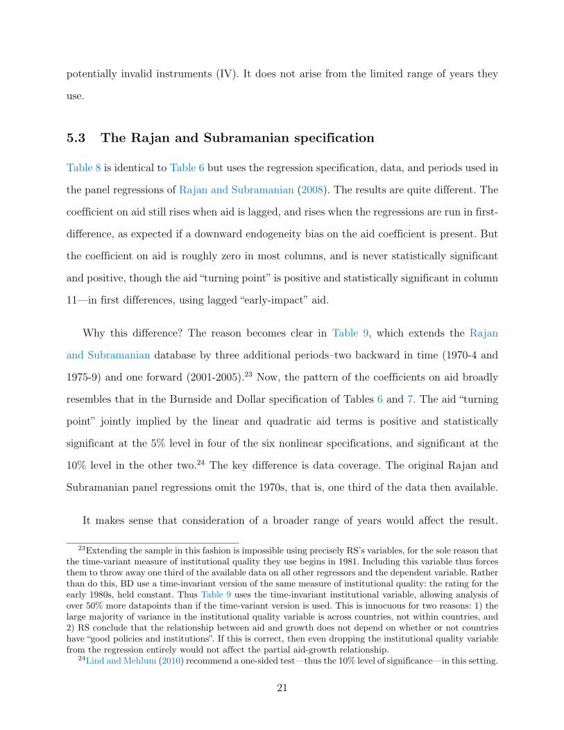
5.3 The Rajan and Subramanian specification

Table 8 is identical to Table 6 but uses the regression specification, data, and periods used in

the panel regressions of Rajan and Subramanian (2008). The results are quite different. The

coefficient on aid still rises when aid is lagged, and rises when the regressions are run in first-

difference, as expected if a downward endogeneity bias on the aid coefficient is present. But

the coefficient on aid is roughly zero in most columns, and is never statistically significant

and positive, though the aid “turning point” is positive and statistically significant in column

11—in first differences, using lagged “early-impact” aid.

Why this difference? The reason becomes clear in Table 9, which extends the Rajan

and Subramanian database by three additional periods–two backward in time (1970-4 and

1975-9) and one forward (2001-2005).23 Now, the pattern of the coefficients on aid broadly

resembles that in the Burnside and Dollar specification of Tables 6 and 7. The aid “turning

point” jointly implied by the linear and quadratic aid terms is positive and statistically

significant at the 5% level in four of the six nonlinear specifications, and significant at the

10% level in the other two.24 The key difference is data coverage. The original Rajan and

Subramanian panel regressions omit the 1970s, that is, one third of the data then available.

It makes sense that consideration of a broader range of years would affect the result.

23Extending the sample in this fashion is impossible using precisely RS’s variables, for the sole reason thatthe time-variant measure of institutional quality they use begins in 1981. Including this variable thus forcesthem to throw away one third of the available data on all other regressors and the dependent variable. Ratherthan do this, BD use a time-invariant version of the same measure of institutional quality: the rating for theearly 1980s, held constant. Thus Table 9 uses the time-invariant institutional variable, allowing analysis ofover 50% more datapoints than if the time-variant version is used. This is innocuous for two reasons: 1) thelarge majority of variance in the institutional quality variable is across countries, not within countries, and2) RS conclude that the relationship between aid and growth does not depend on whether or not countrieshave “good policies and institutions”. If this is correct, then even dropping the institutional quality variablefrom the regression entirely would not affect the partial aid-growth relationship.

24Lind and Mehlum (2010) recommend a one-sided test—thus the 10% level of significance—in this setting.

21

The debt crisis of the 1980s, the crisis of the Heavily Indebted Poor Countries (HIPC) in

the 1990s, and destabilization following the end of the Cold War in the 1990s were times

of generally poor growth in developing countries, and the original Rajan and Subramanian

panel regressions treat only those years. Conditions were more favorable in the 1970s and

the early 2000s, years included in the regressions of Table 9. When these years are included

in the sample, the pattern of coefficients on aid in the Rajan and Subramanian specifications

(Table 9) does not materially differ from the pattern in the Burnside and Dollar specifications

(Table 7). These show an aid coefficient roughly in the range 0.15-0.40.

The results in Table 9 are not necessarily incompatible with Rajan and Subramanian’s

conclusion that “the predicted positive effects of aid inflows on growth are likely to be smaller

than suggested by advocates”. While some advocates claim a large relationship, the results

in this and other tables herein show a relationship that is modest rather than large. These

results do not, however, offer grounds for Rajan and Subramanian’s strong conclusion that

aid and growth have no detectable relationship whatsoever or that the cross-country data

may be purely “noise”. They suggest that Rajan and Subramanian’s null result might be

attributable to 1) the limited sample of years in their panel regressions, 2) their restriction

in most regressions that the aid effect be linear,25 3) a failure to identify the causal portion

of the aid-growth relationship in their panel regressions due to weak instruments, and 4)

a failure to identify the causal portion of the aid-growth relationship in their cross-section

regressions, due to reliance on a single instrument (population size) that is weak in nonlinear

specifications and plausibly invalid in all specifications.26

25As mentioned above, instrumentation is very weak in all of Rajan and Subramanian’s published regres-sions that allow for a nonlinear effect (Bazzi and Clemens 2010). In two of their panel regressions where aidis instrumented RS do include a squared term, but this only aggravates the problem of instrument weakness.

26Arndt et al. (2010) corroborate some of these issues with the Rajan and Subramanian specification, anddiscuss others.

22

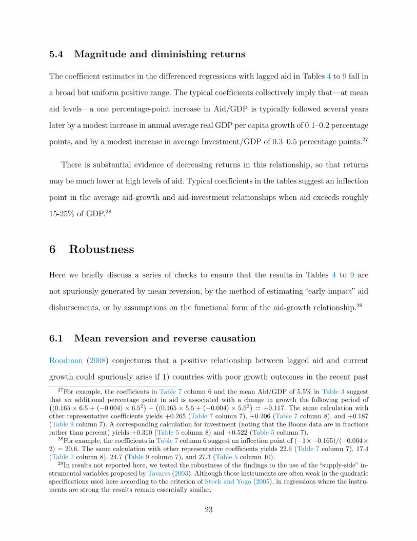
5.4 Magnitude and diminishing returns

The coefficient estimates in the differenced regressions with lagged aid in Tables 4 to 9 fall in

a broad but uniform positive range. The typical coefficients collectively imply that—at mean

aid levels—a one percentage-point increase in Aid/GDP is typically followed several years

later by a modest increase in annual average real GDP per capita growth of 0.1–0.2 percentage

points, and by a modest increase in average Investment/GDP of 0.3–0.5 percentage points.27

There is substantial evidence of decreasing returns in this relationship, so that returns

may be much lower at high levels of aid. Typical coefficients in the tables suggest an inflection

point in the average aid-growth and aid-investment relationships when aid exceeds roughly

15-25% of GDP.28

6 Robustness

Here we briefly discuss a series of checks to ensure that the results in Tables 4 to 9 are

not spuriously generated by mean reversion, by the method of estimating “early-impact” aid

disbursements, or by assumptions on the functional form of the aid-growth relationship.29

6.1 Mean reversion and reverse causation

Roodman (2008) conjectures that a positive relationship between lagged aid and current

growth could spuriously arise if 1) countries with poor growth outcomes in the recent past

27For example, the coefficients in Table 7 column 6 and the mean Aid/GDP of 5.5% in Table 3 suggestthat an additional percentage point in aid is associated with a change in growth the following period of((0.165 × 6.5 + (−0.004) × 6.52

)−

((0.165 × 5.5 + (−0.004) × 5.52

)= +0.117. The same calculation with

other representative coefficients yields +0.265 (Table 7 column 7), +0.206 (Table 7 column 8), and +0.187(Table 9 column 7). A corresponding calculation for investment (noting that the Boone data are in fractionsrather than percent) yields +0.310 (Table 5 column 8) and +0.522 (Table 5 column 7).

28For example, the coefficients in Table 7 column 6 suggest an inflection point of (−1×−0.165)/(−0.004×2) = 20.6. The same calculation with other representative coefficients yields 22.6 (Table 7 column 7), 17.4(Table 7 column 8), 24.7 (Table 9 column 7), and 27.3 (Table 5 column 10).

29In results not reported here, we tested the robustness of the findings to the use of the “supply-side” in-strumental variables proposed by Tavares (2003). Although those instruments are often weak in the quadraticspecifications used here according to the criterion of Stock and Yogo (2005), in regressions where the instru-ments are strong the results remain essentially similar.

23

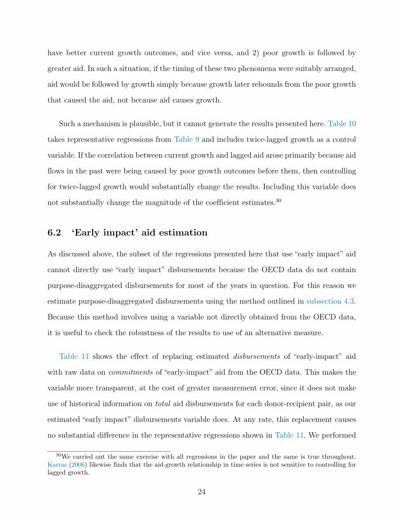
have better current growth outcomes, and vice versa, and 2) poor growth is followed by

greater aid. In such a situation, if the timing of these two phenomena were suitably arranged,

aid would be followed by growth simply because growth later rebounds from the poor growth

that caused the aid, not because aid causes growth.

Such a mechanism is plausible, but it cannot generate the results presented here. Table 10

takes representative regressions from Table 9 and includes twice-lagged growth as a control

variable. If the correlation between current growth and lagged aid arose primarily because aid

flows in the past were being caused by poor growth outcomes before them, then controlling

for twice-lagged growth would substantially change the results. Including this variable does

not substantially change the magnitude of the coefficient estimates.30

6.2 ‘Early impact’ aid estimation

As discussed above, the subset of the regressions presented here that use “early impact” aid

cannot directly use “early impact” disbursements because the OECD data do not contain

purpose-disaggregated disbursements for most of the years in question. For this reason we

estimate purpose-disaggregated disbursements using the method outlined in subsection 4.3.

Because this method involves using a variable not directly obtained from the OECD data,

it is useful to check the robustness of the results to use of an alternative measure.

Table 11 shows the effect of replacing estimated disbursements of “early-impact” aid

with raw data on commitments of “early-impact” aid from the OECD data. This makes the

variable more transparent, at the cost of greater measurement error, since it does not make

use of historical information on total aid disbursements for each donor-recipient pair, as our

estimated “early impact” disbursements variable does. At any rate, this replacement causes

no substantial difference in the representative regressions shown in Table 11. We performed

30We carried out the same exercise with all regressions in the paper and the same is true throughout.Karras (2006) likewise finds that the aid-growth relationship in time series is not sensitive to controlling forlagged growth.

24

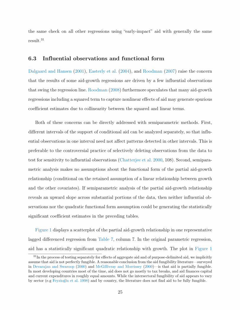
the same check on all other regressions using “early-impact” aid with generally the same

result.31

6.3 Influential observations and functional form

Dalgaard and Hansen (2001), Easterly et al. (2004), and Roodman (2007) raise the concern

that the results of some aid-growth regressions are driven by a few influential observations

that swing the regression line. Roodman (2008) furthermore speculates that many aid-growth

regressions including a squared term to capture nonlinear effects of aid may generate spurious

coefficient estimates due to collinearity between the squared and linear terms.

Both of these concerns can be directly addressed with semiparametric methods. First,

different intervals of the support of conditional aid can be analyzed separately, so that influ-

ential observations in one interval need not affect patterns detected in other intervals. This is

preferable to the controversial practice of selectively deleting observations from the data to

test for sensitivity to influential observations (Chatterjee et al. 2000, 108). Second, semipara-

metric analysis makes no assumptions about the functional form of the partial aid-growth

relationship (conditional on the retained assumption of a linear relationship between growth

and the other covariates). If semiparametric analysis of the partial aid-growth relationship

reveals an upward slope across substantial portions of the data, then neither influential ob-

servations nor the quadratic functional form assumption could be generating the statistically

significant coefficient estimates in the preceding tables.

Figure 1 displays a scatterplot of the partial aid-growth relationship in one representative

lagged differenced regression from Table 7, column 7. In the original parametric regression,

aid has a statistically significant quadratic relationship with growth. The plot in Figure 1

31In the process of testing separately for effects of aggregate aid and of purpose-delimited aid, we implicitlyassume that aid is not perfectly fungible. A reasonable conclusion from the aid fungibility literature—surveyedin Devarajan and Swaroop (2000) and McGillivray and Morrissey (2000)—is that aid is partially fungible.In most developing countries most of the time, aid does not go mostly to tax breaks, and aid finances capitaland current expenditures in roughly equal amounts. While the intersectoral fungibility of aid appears to varyby sector (e.g Feyzioglu et al. 1998) and by country, the literature does not find aid to be fully fungible.

25

partials out the same non-aid covariates from growth (vertical axis) and aid (horizontal axis).

The figure shows that the positive partial correlation in the parametric regression result is

not produced by one or two influential observations, and is not generated spuriously by the

assumption of a quadratic partial relationship between aid and growth.

7 Conclusions

These results imply that straightforward changes to the research designs of the most cited

papers in the aid-growth literature move us closer to resolving the divergence between their

findings. There is one broad finding from the regression specifications used in all of these

studies: Aid inflows are systematically associated with modest, positive subsequent growth

in cross-country panel data. The principal reasons that other studies have not observed this

relationship are that they tested for aid effects within an inappropriate time horizon, relied

too much on weak or invalid instrumental variables, and looked at historical time series that

were too short.

Most of the substantial disagreements in the literature’s most influential studies disappear

when aid is allowed to affect growth with a lag, when only portions of aid relevant to short-

term growth are tested for short-term growth effects, and when the historical time series

under observation is extended to include all available data. This finding does not depend on

assumptions about the functional form of the aid-growth relationship, does not arise from a

handful of influential observations, and is not an artifact of mean reversion.

Clearly, the fact that increases in aid are typically followed by increases in growth is a

necessary but not sufficient condition to demonstrate scientifically that aid causes growth.

There are related debates about the direction of causality between investment and growth,

savings and growth, health outcomes and growth, and institutions and growth, to name a

few. In other words, Granger causality does not strictly imply true causality. As we point

out, however, the aid-growth literature does not currently possess a strong and patently

26

valid instrumental variable with which to reliably test the hypothesis that aid strictly causes

growth, raising significant doubts about the conclusions of the studies that have relied on

instrumentation. The most plausible explanation for the fact that aid increases are systemat-

ically followed by growth increases on average is that aid does cause modest positive increases

in growth on average. There is little empirical support for the notion that aid systematically

reduces growth (Temple 2010).

The results do not by any means imply that aid “works” everywhere, or even in the

median country. First, even if “working” is taken to mean contributing to economic growth,

a universal trait of aid-growth analyses (and growth studies more broadly) is that a very

large number of countries lie well above and well below the regression line; it is clear that in

many countries, even large aid inflows have been insufficient to spark growth over any time

horizon. Second, there are many other metrics against which aid could be judged to “work”

even if there were no growth impact; the aid money that supported the smallpox eradication

campaign accomplished its goal, whether or not that campaign’s success will ever be felt in

the national accounts. Finally, aid appears to have a nonlinear effect on growth, and there

may be limits on the degree to which even large aid receipts can further increase growth in

the typical recipient (Gupta and Heller 2002).

These results do not suggest that aid can or should be the main driver of growth. As

Kraay (2006) points out, far more of the variance in growth across countries is accounted

for by the non-aid covariates in these regressions than by the aid variable. Many important

growth successes across the developing world have been accomplished with relatively little

foreign aid, such as in post-Mao China and post-renovation (Đổi Mới) Vietnam. But the

findings do suggest that on average—over all countries, over many decades, and regardless

of the regression specification—aid has had a modest positive effect on growth.

27

References

Anderson, T.W. and Cheng Hsiao, “Formulation and estimation of dynamic modelsusing panel data,” Journal of econometrics, 1982, 18 (1), 47–82.

Arndt, Channing, Sam Jones, and Finn Tarp, “Aid, Growth, and Development: HaveWe Come Full Circle?,” Journal of Globalization and Development, 2010, 1 (2), 5.

Barro, Robert J., Determinants of Economic Growth: A Cross-Country Empirical Study,Cambridge, Mass.: The MIT Press, 1997.

Batista, Catia and Juan Zalduendo, “Can the IMF’s Medium-Term Growth ProjectionsBe Improved?,” IMF Working Papers 04/203, International Monetary Fund 2004.

Bazzi, Samuel and Michael A. Clemens, “Blunt Instruments: A cautionary note onestablishing the causes of economic growth,” Working Papers 171, Center for Global De-velopment 2010.

Boone, Peter, “Politics and the effectiveness of foreign aid,” European Economic Review,1996, 40 (2), 289–329.

Burnside, Craig and David Dollar, “Aid, Policies, and Growth,” American EconomicReview, 2000, 90 (4), 847–868.

and , “Aid, policies, and growth : revisiting the evidence,” Policy Research WorkingPaper Series 3251, The World Bank 2004.

Chang, Charles C., Eduardo Fernández-Arias, and Luís Servén, “Measuring aidflows: a new approach,” Policy Research Working Paper Series 2050, The World Bank1999.

Chatterjee, Samprit, Ali S. Hadi, and Bertram Price, Regression Analysis by Exam-ple, New York: John Wiley and Sons, Inc.), 2000.

Chauvet, Lisa and Patrick Guillaumont, “Aid and Growth Revisited : Policy, EconomicVulnerability and Political Instability,” in Bertil Tungodden, Nicholas Stern, and IvarKolstad, eds., Towards Pro-Poor Policies: Aid, Institutions, and Globalization, Oxford:Oxford University Press, 2004.

Clemens, Michael A., Steven Radelet, and Rikhil R. Bhavnani, “Counting ChickensWhen They Hatch: The Short-term Effect of Aid on Growth,” Working Paper 44, Centerfor Global Development 2004.

Collier, Paul and Anke Hoeffler, “Aid, policy and growth in post-conflict societies,”European Economic Review, 2004, 48 (5), 1125–1145.

and David Dollar, “Aid allocation and poverty reduction,” European Economic Review,2002, 46 (8), 1475–1500.

28

and Jan Dehn, “Aid, shocks, and growth,” Policy Research Working Paper Series 2688,The World Bank 2001.

Cragg, John G. and Stephen G. Donald, “Testing Identifiability and Specification inInstrumental Variable Models,” Econometric Theory, 1993, 9 (02), 222–240.

Dalgaard, Carl-Johan and Henrik Hansen, “On aid, growth and good policies,” Journalof Development Studies, 2001, 37 (6), 17–41.

, , and Finn Tarp, “On The Empirics of Foreign Aid and Growth,” Economic Journal,2004, 114 (496), F191–F216.

Devarajan, Shantayanan and Vinaya Swaroop, “The Implications of Foreign Aid Fun-gibility for Development Assistance,” in Christopher L. Gilbert and David Vines, eds., TheWorld Bank: Structure and Policies, New York: Cambridge University Press, 2000.

Djankov, Simeon, Jose Montalvo, and Marta Reynal-Querol, “The curse of aid,”Journal of Economic Growth, 2008, 13 (3), 169–194.

Dreher, Axel, Peter Nunnenkamp, and Rainer Thiele, “Does aid for education ed-ucate children? Evidence from panel data,” The World Bank Economic Review, 2008, 22(2), 291.

Durlauf, Steven N. and Danny T. Quah, “The new empirics of economic growth,” inJohn Taylor and Michael Woodford, eds., Handbook of Macroeconomics, Vol. 1A, Amster-dam: North-Holland, 1999.

Easterly, William, “Can Foreign Aid Buy Growth?,” Journal of Economic Perspectives,2003, 17 (3), 23–48.

, The White Man’s Burden: Why the West’s Efforts to Aid the Rest Have Done So MuchIll and So Little Good, New York: The Penguin Press, 2006.

, Michael Kremer, Lant Pritchett, and Lawrence H. Summers, “Good policy orgood luck?: Country growth performance and temporary shocks,” Journal of MonetaryEconomics, 1993, 32 (3), 459–483.

, Ross Levine, and David Roodman, “Aid, Policies, and Growth: Comment,” AmericanEconomic Review, 2004, 94 (3), 774–780.

Feyzioglu, Tarhan, Vinaya Swaroop, and Min Zhu, “A Panel Data Analysis of theFungibility of Foreign Aid,” World Bank Economic Review, 1998, 12 (1), 29–58.

Frankel, Jeffrey A. and David Romer, “Does trade cause growth?,” American EconomicReview, 1999, 89 (3), 379–399.

Granger, Clive W. J., “Investigating Causal Relations by Econometric Models and Cross-Spectral Methods,” Econometrica, 1969, 37 (3), 424–38.

29

Griffin, Keith B. and J. L. Enos, “Foreign Assistance: Objectives and Consequences,”Economic Development and Cultural Change, 1970, 18 (3), 313–27.

Guillaumont, Patrick and Lisa Chauvet, “Aid and performance: a reassessment,” Jour-nal of Development Studies, 2001, 37 (6), 66–92.

Gulati, Umesh C, “Effect of Capital Imports on Savings and Growth in Less DevelopedCountries,” Economic Inquiry, 1978, 16 (4), 563–69.

Gupta, Kanhaya L. and M. Anisul Islam, Foreign capital, savings and growth: Aninternational cross-section study, International Studies in Economics and Econometrics,Vol. 9), publisher=D. Reidel Pub. Co., address=Boston 1983.

Gupta, Sanjeev and Peter S. Heller, “Challenges in Expanding Development Assis-tance,” IMF Policy Discussion Papers 02/5, International Monetary Fund 2002.

Hadjimichael, Michael T., Dhaneshwar Ghura, Martin Muhleisen, Roger Nord,and E. Murat Ucer, “Sub-Saharan Africa: Growth, Savings, and Investment, 1986-93,”IMF Occasional Papers 118, International Monetary Fund 1995.

Hansen, Henrik and Finn Tarp, “Aid effectiveness disputed,” Journal of InternationalDevelopment, 2000, 12 (3), 375–398.

and , “Aid and growth regressions,” Journal of Development Economics, 2001, 64 (2),547–570.

Hausmann, Ricardo, Jason Hwang, and Dani Rodrik, “What you export matters,”Journal of Economic Growth, 2007, 12 (1), 1–25.

Islam, Muhammed N., “Political regimes and the effects of foreign aid on economicgrowth,” The Journal of Developing Areas, 2003, 37 (1), 35–53.

Islam, Nazrul, “Growth Empirics: A Panel Data Approach,” The Quarterly Journal ofEconomics, 1995, 110 (4), 1127–70.

, “What have We Learnt from the Convergence Debate?,” Journal of Economic Surveys,2003, 17 (3), 309–362.

Karras, Georgios, “Foreign aid and long-run economic growth: empirical evidence for apanel of developing countries,” Journal of International Development, 2006, 18 (1), 15–28.

Kleibergen, Frank and Richard Paap, “Generalized reduced rank tests using the singularvalue decomposition,” Journal of Econometrics, 2006, 133 (1), 97–126.

Knack, Stephen and Aminur Rahman, “Donor fragmentation and bureaucratic qualityin aid recipients,” Journal of Development Economics, 2007, 83 (1), 176–197.

Kraay, Aart, “Aid, growth, and poverty,” in Peter Isard, Leslie Lipschitz, Alexandros Mour-mouras, and Boriana Yontcheva, eds., The Macroeconomic Management of Foreign Aid:Opportunities and Pitfalls, Washington, DC: International Monetary Fund, 2006.

30

Lensink, Robert and Howard White, “Are there negative returns to aid?,” Journal ofdevelopment Studies, 2001, 37 (6), 42–65.

and Oliver Morrissey, “Aid instability as a measure of uncertainty and the positiveimpact of aid on growth,” Journal of Development Studies, 2000, 36 (3), 31–49.

Levy, Victor, “Aid and growth in Sub-Saharan Africa: The recent experience,” EuropeanEconomic Review, 1988, 32 (9), 1777–1795.

Lind, Jo Thori and Halvor Mehlum, “With or Without U? The Appropriate Test for aU-Shaped Relationship,” Oxford Bulletin of Economics and Statistics, 2010, 72 (1), 109–118.

Mavrotas, George, “Aid and growth in India: some evidence from disaggregated aid data,”South Asia Economic Journal, 2002, 3 (1), 19–49.

McGillivray, Mark and Oliver Morrissey, “Aid fungibility in Assessing Aid: red herringor true concern?,” Journal of International Development, 2000, 12 (3), 413–428.

Mehrhoff, Jens, “A solution to the problem of too many instruments in dynamic paneldata GMM,” Discussion Paper Series 1, Economic Studies 31/2009, Deutsche Bundesbank2009.

Moreira, S.B., “Evaluating the Impact of Foreign Aid on Economic Growth: A Cross-Country Study,” Journal of Economic Development, 2005, 30 (2), 25–48.

Mosley, Paul, “Aid, Savings and Growth Revisited,” Oxford Bulletin of Economics andStatistics, 1980, 42 (2), 79–95.

, John Hudson, and Sara Horrell, “Aid, the Public Sector and the Market in LessDeveloped Countries,” Economic Journal, 1987, 97 (387), 616–41.

Nickell, Stephen J., “Biases in Dynamic Models with Fixed Effects,” Econometrica, 1981,49 (6), 1417–26.

Over, Mead, “An Example of the Simultaneous-Equation Problem: A Note on ‘ForeignAssistance: Objectives and Consequences’,” Economic Development and Cultural Change,1975, 23 (4), 751–756.

Owens, Trudy and John Hoddinott, “Investing in development or investing in relief:Quantifying the poverty tradeoffs using Zimbabwe household panel data,” Working Paper99-4, Oxford Centre for the Study of African Economies 1999.

Papanek, Gustav F., “The Effect of Aid and other Resource Transfers on Savings andGrowth in Less Developed Countries,” Economic Journal, 1972, 82 (327), 934–50.

, “Aid, Foreign Private Investment, Savings, and Growth in Less Developed Countries,”Journal of Political Economy, 1973, 81 (1), 120–30.

31

Rajan, Raghuram G. and Arvind Subramanian, “Aid and Growth: What Does theCross-Country Evidence Really Show?,” The Review of Economics and Statistics, 2008,90 (4), 643–665.

Roodman, David, “The Anarchy of Numbers: Aid, Development, and Cross-Country Em-pirics,” World Bank Economic Review, 2007, 21 (2), 255–277.

, “Through the looking glass, and what ols found there: on growth, foreign aid, and reversecausality,” Working Paper 137, Center for Global Development 2008.

, “A Note on the Theme of Too Many Instruments,” Oxford Bulletin of Economics andStatistics, 2009, 71 (1), 135–158.

Spolaore, Enrico and Romain Wacziarg, “Borders and Growth,” Journal of EconomicGrowth, 2005, 10 (4), 331–386.

Stock, James H. and Motohiro Yogo, “Testing for weak instruments in linear IV regres-sion,” in Donald W. K. Andrews and James H. Stock, eds., Identification and Inference forEconometric Models: Essays in Honor of Thomas J. Rothenberg, New York: CambridgeUniversity Press, 2005.

Tavares, José, “Does foreign aid corrupt?,” Economics Letters, 2003, 79 (1), 99–106.

Temple, Jonathan, “The New Growth Evidence,” Journal of Economic Literature, 1999,37 (1), 112–156.

Temple, Jonathan R.W., “Aid and Conditionality,” in Dani Rodrik and Mark Rosenzweig,eds., Handbooks in Economics, Vol. 5 of Handbook of Development Economics, Elsevier,2010, pp. 4415–4523.

Weisskopf, Thomas E., “The impact of foreign capital inflow on domestic savings inunderdeveloped countries,” Journal of International Economics, 1972, 2 (1), 25–38.

Werker, Eric, Faisal Z. Ahmed, and Charles Cohen, “How Is Foreign Aid Spent?Evidence from a Natural Experiment,” American Economic Journal: Macroeconomics,2009, 1 (2), 225–44.

32

Table 1: Previous studies rely on population size for instrument strength

BooneBurnside Rajan andand Dollar Subramanian

Population IVs in 2nd stagea — Yes — Yes Yes — YesPolicy IVs in 2nd stageb — — — — Yes — —

Cragg-Donald F -stat 15.70 1.77 19.74 7.04 4.65 31.63 0.13Kleibergen-Paap F -stat 7.57 1.69 15.76 5.90 2.77 36.12 0.07Kleibergen-Paap LM stat p-val. < 0.01 0.20 < 0.01 0.06 0.12 < 0.01 0.77

Observations 132 132 275 275 275 78 78Years 1971-1990 1970-1993 1970-2000

a “Population IVs in 2nd stage” means that the ln(population) instrument is included in the secondstage in the Boone regression and in the Rajan and Subramanian regression. In the Burnside andDollar regression it means that all three instruments containing population are included in the 2ndstage; these are ln(population), ln(population) × ‘policy’, and (ln(population))2 × ‘policy’.

b “Policy IVs in 2nd stage” means that all instruments containing ‘policy’ are included in thesecond stage: These are ln(initial income) × policy, (ln(initial income)2) × policy, and (laggedarms imports/total imports) × policy. The regressions replicated and modified are Boone (1996)Table 4, column V, row 3; Burnside and Dollar (2000) Table 4, column 3 2SLS; and Rajan andSubramanian (2008) Table 4A, column 2.

33

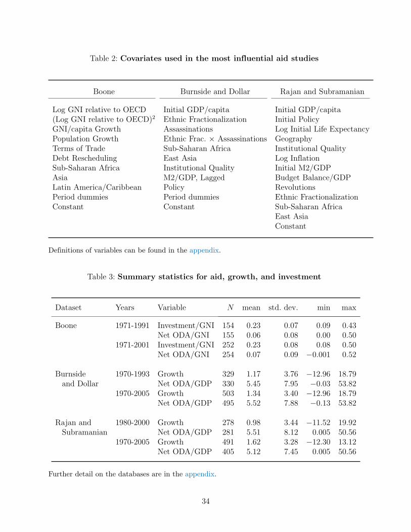
Table 2: Covariates used in the most influential aid studies

Boone Burnside and Dollar Rajan and Subramanian

Log GNI relative to OECD Initial GDP/capita Initial GDP/capita(Log GNI relative to OECD)2 Ethnic Fractionalization Initial PolicyGNI/capita Growth Assassinations Log Initial Life ExpectancyPopulation Growth Ethnic Frac. × Assassinations GeographyTerms of Trade Sub-Saharan Africa Institutional QualityDebt Rescheduling East Asia Log InflationSub-Saharan Africa Institutional Quality Initial M2/GDPAsia M2/GDP, Lagged Budget Balance/GDPLatin America/Caribbean Policy RevolutionsPeriod dummies Period dummies Ethnic FractionalizationConstant Constant Sub-Saharan Africa

East AsiaConstant

Definitions of variables can be found in the appendix.

Table 3: Summary statistics for aid, growth, and investment

Dataset Years Variable N mean std. dev. min max

Boone 1971-1991 Investment/GNI 154 0.23 0.07 0.09 0.43Net ODA/GNI 155 0.06 0.08 0.00 0.50

1971-2001 Investment/GNI 252 0.23 0.08 0.08 0.50Net ODA/GNI 254 0.07 0.09 −0.001 0.52

Burnside 1970-1993 Growth 329 1.17 3.76 −12.96 18.79and Dollar Net ODA/GDP 330 5.45 7.95 −0.03 53.82

1970-2005 Growth 503 1.34 3.40 −12.96 18.79Net ODA/GDP 495 5.52 7.88 −0.13 53.82

Rajan and 1980-2000 Growth 278 0.98 3.44 −11.52 19.92Subramanian Net ODA/GDP 281 5.51 8.12 0.005 50.56

1970-2005 Growth 491 1.62 3.28 −12.30 13.12Net ODA/GDP 405 5.12 7.45 0.005 50.56

Further detail on the databases are in the appendix.

34

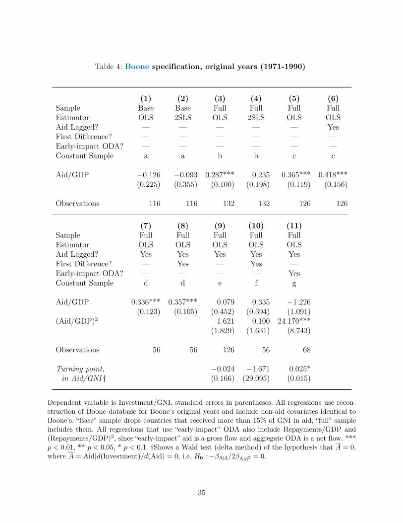
Table 4: Boone specification, original years (1971-1990)

(1) (2) (3) (4) (5) (6)Sample Base Base Full Full Full FullEstimator OLS 2SLS OLS 2SLS OLS OLSAid Lagged? — — — — — YesFirst Difference? — — — — — —Early-impact ODA? — — — — — —Constant Sample a a b b c c

Aid/GDP −0.126 −0.093 0.287*** 0.235 0.365*** 0.418***(0.225) (0.355) (0.100) (0.198) (0.119) (0.156)

Observations 116 116 132 132 126 126

(7) (8) (9) (10) (11)Sample Full Full Full Full FullEstimator OLS OLS OLS OLS OLSAid Lagged? Yes Yes Yes Yes YesFirst Difference? — Yes — Yes —Early-impact ODA? — — — — YesConstant Sample d d e f g

Aid/GDP 0.336*** 0.357*** 0.079 0.335 −1.226(0.123) (0.105) (0.452) (0.394) (1.091)

(Aid/GDP)2 1.621 0.100 24.170***(1.829) (1.631) (8.743)

Observations 56 56 126 56 68

Turning point, −0.024 −1.671 0.025*in Aid/GNI † (0.166) (29.095) (0.015)

Dependent variable is Investment/GNI, standard errors in parentheses. All regressions use recon-struction of Boone database for Boone’s original years and include non-aid covariates identical toBoone’s. “Base” sample drops countries that received more than 15% of GNI in aid, “full” sampleincludes them. All regressions that use “early-impact” ODA also include Repayments/GDP and(Repayments/GDP)2, since “early-impact” aid is a gross flow and aggregate ODA is a net flow. ***p < 0.01, ** p < 0.05, * p < 0.1. †Shows a Wald test (delta method) of the hypothesis that A = 0,where A = Aid|d(Investment)/d(Aid) = 0, i.e. H0 : −βAid/2βAid2 = 0.

35

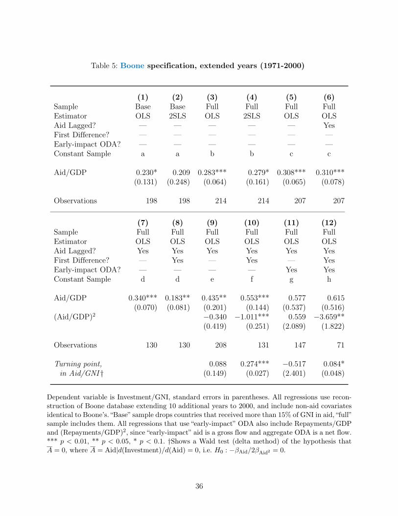
Table 5: Boone specification, extended years (1971-2000)

(1) (2) (3) (4) (5) (6)Sample Base Base Full Full Full FullEstimator OLS 2SLS OLS 2SLS OLS OLSAid Lagged? — — — — — YesFirst Difference? — — — — — —Early-impact ODA? — — — — — —Constant Sample a a b b c c

Aid/GDP 0.230* 0.209 0.283*** 0.279* 0.308*** 0.310***(0.131) (0.248) (0.064) (0.161) (0.065) (0.078)

Observations 198 198 214 214 207 207

(7) (8) (9) (10) (11) (12)Sample Full Full Full Full Full FullEstimator OLS OLS OLS OLS OLS OLSAid Lagged? Yes Yes Yes Yes Yes YesFirst Difference? — Yes — Yes — YesEarly-impact ODA? — — — — Yes YesConstant Sample d d e f g h

Aid/GDP 0.340*** 0.183** 0.435** 0.553*** 0.577 0.615(0.070) (0.081) (0.201) (0.144) (0.537) (0.516)

(Aid/GDP)2 −0.340 −1.011*** 0.559 −3.659**(0.419) (0.251) (2.089) (1.822)

Observations 130 130 208 131 147 71

Turning point, 0.088 0.274*** −0.517 0.084*in Aid/GNI † (0.149) (0.027) (2.401) (0.048)

Dependent variable is Investment/GNI, standard errors in parentheses. All regressions use recon-struction of Boone database extending 10 additional years to 2000, and include non-aid covariatesidentical to Boone’s. “Base” sample drops countries that received more than 15% of GNI in aid, “full”sample includes them. All regressions that use “early-impact” ODA also include Repayments/GDPand (Repayments/GDP)2, since “early-impact” aid is a gross flow and aggregate ODA is a net flow.*** p < 0.01, ** p < 0.05, * p < 0.1. †Shows a Wald test (delta method) of the hypothesis thatA = 0, where A = Aid|d(Investment)/d(Aid) = 0, i.e. H0 : −βAid/2βAid2 = 0.

36

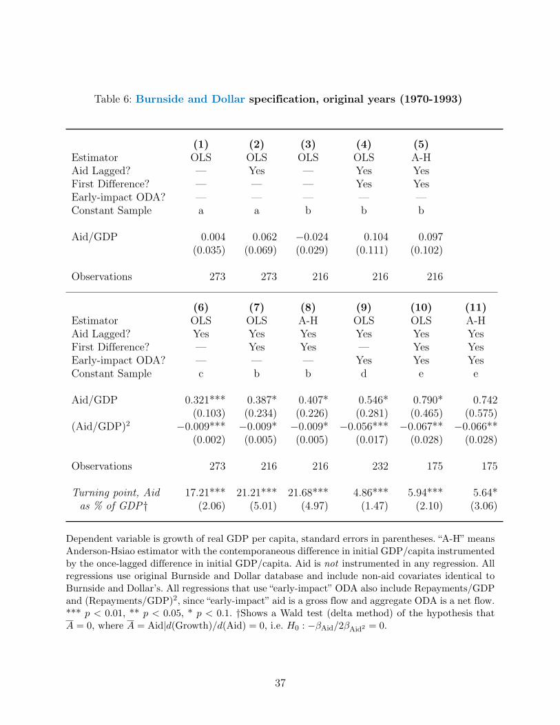
Table 6: Burnside and Dollar specification, original years (1970-1993)

(1) (2) (3) (4) (5)Estimator OLS OLS OLS OLS A-HAid Lagged? — Yes — Yes YesFirst Difference? — — — Yes YesEarly-impact ODA? — — — — —Constant Sample a a b b b

Aid/GDP 0.004 0.062 −0.024 0.104 0.097(0.035) (0.069) (0.029) (0.111) (0.102)

Observations 273 273 216 216 216

(6) (7) (8) (9) (10) (11)Estimator OLS OLS A-H OLS OLS A-HAid Lagged? Yes Yes Yes Yes Yes YesFirst Difference? — Yes Yes — Yes YesEarly-impact ODA? — — — Yes Yes YesConstant Sample c b b d e e

Aid/GDP 0.321*** 0.387* 0.407* 0.546* 0.790* 0.742(0.103) (0.234) (0.226) (0.281) (0.465) (0.575)

(Aid/GDP)2 −0.009*** −0.009* −0.009* −0.056*** −0.067** −0.066**(0.002) (0.005) (0.005) (0.017) (0.028) (0.028)

Observations 273 216 216 232 175 175

Turning point, Aid 17.21*** 21.21*** 21.68*** 4.86*** 5.94*** 5.64*as % of GDP† (2.06) (5.01) (4.97) (1.47) (2.10) (3.06)

Dependent variable is growth of real GDP per capita, standard errors in parentheses. “A-H” meansAnderson-Hsiao estimator with the contemporaneous difference in initial GDP/capita instrumentedby the once-lagged difference in initial GDP/capita. Aid is not instrumented in any regression. Allregressions use original Burnside and Dollar database and include non-aid covariates identical toBurnside and Dollar’s. All regressions that use “early-impact” ODA also include Repayments/GDPand (Repayments/GDP)2, since “early-impact” aid is a gross flow and aggregate ODA is a net flow.*** p < 0.01, ** p < 0.05, * p < 0.1. †Shows a Wald test (delta method) of the hypothesis thatA = 0, where A = Aid|d(Growth)/d(Aid) = 0, i.e. H0 : −βAid/2βAid2 = 0.

37

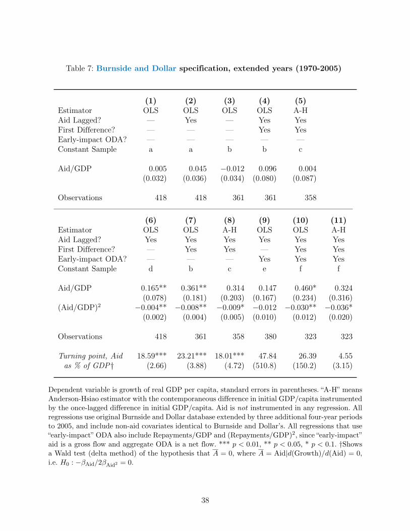
Table 7: Burnside and Dollar specification, extended years (1970-2005)

(1) (2) (3) (4) (5)Estimator OLS OLS OLS OLS A-HAid Lagged? — Yes — Yes YesFirst Difference? — — — Yes YesEarly-impact ODA? — — — — —Constant Sample a a b b c

Aid/GDP 0.005 0.045 −0.012 0.096 0.004(0.032) (0.036) (0.034) (0.080) (0.087)

Observations 418 418 361 361 358

(6) (7) (8) (9) (10) (11)Estimator OLS OLS A-H OLS OLS A-HAid Lagged? Yes Yes Yes Yes Yes YesFirst Difference? — Yes Yes — Yes YesEarly-impact ODA? — — — Yes Yes YesConstant Sample d b c e f f

Aid/GDP 0.165** 0.361** 0.314 0.147 0.460* 0.324(0.078) (0.181) (0.203) (0.167) (0.234) (0.316)

(Aid/GDP)2 −0.004** −0.008** −0.009* −0.012 −0.030** −0.036*(0.002) (0.004) (0.005) (0.010) (0.012) (0.020)

Observations 418 361 358 380 323 323

Turning point, Aid 18.59*** 23.21*** 18.01*** 47.84 26.39 4.55as % of GDP† (2.66) (3.88) (4.72) (510.8) (150.2) (3.15)

Dependent variable is growth of real GDP per capita, standard errors in parentheses. “A-H” meansAnderson-Hsiao estimator with the contemporaneous difference in initial GDP/capita instrumentedby the once-lagged difference in initial GDP/capita. Aid is not instrumented in any regression. Allregressions use original Burnside and Dollar database extended by three additional four-year periodsto 2005, and include non-aid covariates identical to Burnside and Dollar’s. All regressions that use“early-impact” ODA also include Repayments/GDP and (Repayments/GDP)2, since “early-impact”aid is a gross flow and aggregate ODA is a net flow. *** p < 0.01, ** p < 0.05, * p < 0.1. †Showsa Wald test (delta method) of the hypothesis that A = 0, where A = Aid|d(Growth)/d(Aid) = 0,i.e. H0 : −βAid/2βAid2 = 0.

38

Table 8: Rajan and Subramanian specification, original years (1981-2000)

(1) (2) (3) (4) (5)Estimator OLS OLS OLS OLS A-HAid Lagged? — Yes — Yes YesFirst Difference? — — — Yes YesEarly-impact ODA? — — — — —Constant Sample a a b b c

Aid/GDP −0.038 −0.019 −0.128*** −0.019 0.158(0.048) (0.052) (0.035) (0.093) (0.193)

Observations 236 236 164 164 161

(6) (7) (8) (9) (10) (11)Estimator OLS OLS A-H OLS OLS A-HAid Lagged? Yes Yes Yes Yes Yes YesFirst Difference? — Yes Yes — Yes YesEarly-impact ODA? — — — Yes Yes YesConstant Sample d b c e f f

Aid/GDP −0.071 −0.098 0.139 −0.011 −0.186 1.907(0.113) (0.159) (0.280) (0.319) (0.428) (2.503)

(Aid/GDP)2 0.002 0.003 0.001 −0.004 −0.005 −0.167(0.004) (0.006) (0.006) (0.030) (0.035) (0.192)

Observations 236 164 161 226 159 158

Turning point, Aid 16.59 52.69 −99.96 −1.27 −20.38 5.72***as % of GDP† (15.64) (95.82) (1078.6) (44.69) (197.7) (1.25)

Dependent variable is growth of real GDP per capita, standard errors in parentheses. “A-H” meansAnderson-Hsiao estimator with the contemporaneous difference in initial GDP/capita instrumentedby the once-lagged difference in initial GDP/capita. Aid is not instrumented in any regression. Allregressions use original Rajan and Subramanian database, and include non-aid covariates identicalto Rajan and Subramanian’s. All regressions that use “early-impact” ODA also include Repay-ments/GDP and (Repayments/GDP)2, since “early-impact” aid is a gross flow and aggregate ODAis a net flow. *** p < 0.01, ** p < 0.05, * p < 0.1. †Shows a Wald test (delta method) of thehypothesis that A = 0, where A = Aid|d(Growth)/d(Aid) = 0, i.e. H0 : −βAid/2βAid2 = 0.

39

Table 9: Rajan and Subramanian specification, extended years (1971-2005)

(1) (2) (3) (4) (5)Estimator OLS OLS OLS OLS A-HAid Lagged? — Yes — Yes YesFirst Difference? — — — Yes YesEarly-impact ODA? — — — — —Constant Sample a a b b c

Aid/GDP −0.009 0.023 −0.031 0.109 0.058(0.035) (0.044) (0.034) (0.083) (0.091)

Observations 404 404 323 323 322

(6) (7) (8) (9) (10) (11)Estimator OLS OLS A-H OLS OLS A-HAid Lagged? Yes Yes Yes Yes Yes YesFirst Difference? — Yes Yes — Yes YesEarly-impact ODA? — — — Yes Yes YesConstant Sample d b c e f f

Aid/GDP 0.106 0.247 0.191 0.380** 0.675** 0.513(0.079) (0.152) (0.166) (0.169) (0.265) (0.384)

(Aid/GDP)2 −0.003 −0.005 −0.004 −0.022 −0.052** −0.042(0.003) (0.004) (0.004) (0.015) (0.023) (0.029)

Observations 404 323 322 343 268 268

Turning point, Aid 16.13** 27.77* 22.58* 8.46*** 6.95*** 6.05***as % of GDP† (6.85) (16.16) (11.63) (3.15) (1.95) (1.79)

Dependent variable is growth of real GDP per capita, standard errors in parentheses. “A-H” meansAnderson-Hsiao estimator with the contemporaneous difference in initial GDP/capita instrumentedby the once-lagged difference in initial GDP/capita. Aid is not instrumented in any regression. Allregressions use original Rajan and Subramanian database extended by three additional five-yearperiods—back to 1971 and forward to 2005—and include non-aid covariates identical to Rajan andSubramanian’s. All regressions that use “early-impact” ODA also include Repayments/GDP and(Repayments/GDP)2, since “early-impact” aid is a gross flow and aggregate ODA is a net flow. ***p < 0.01, ** p < 0.05, * p < 0.1. †Shows a Wald test (delta method) of the hypothesis that A = 0,where A = Aid|d(Growth)/d(Aid) = 0, i.e. H0 : −βAid/2βAid2 = 0.

40

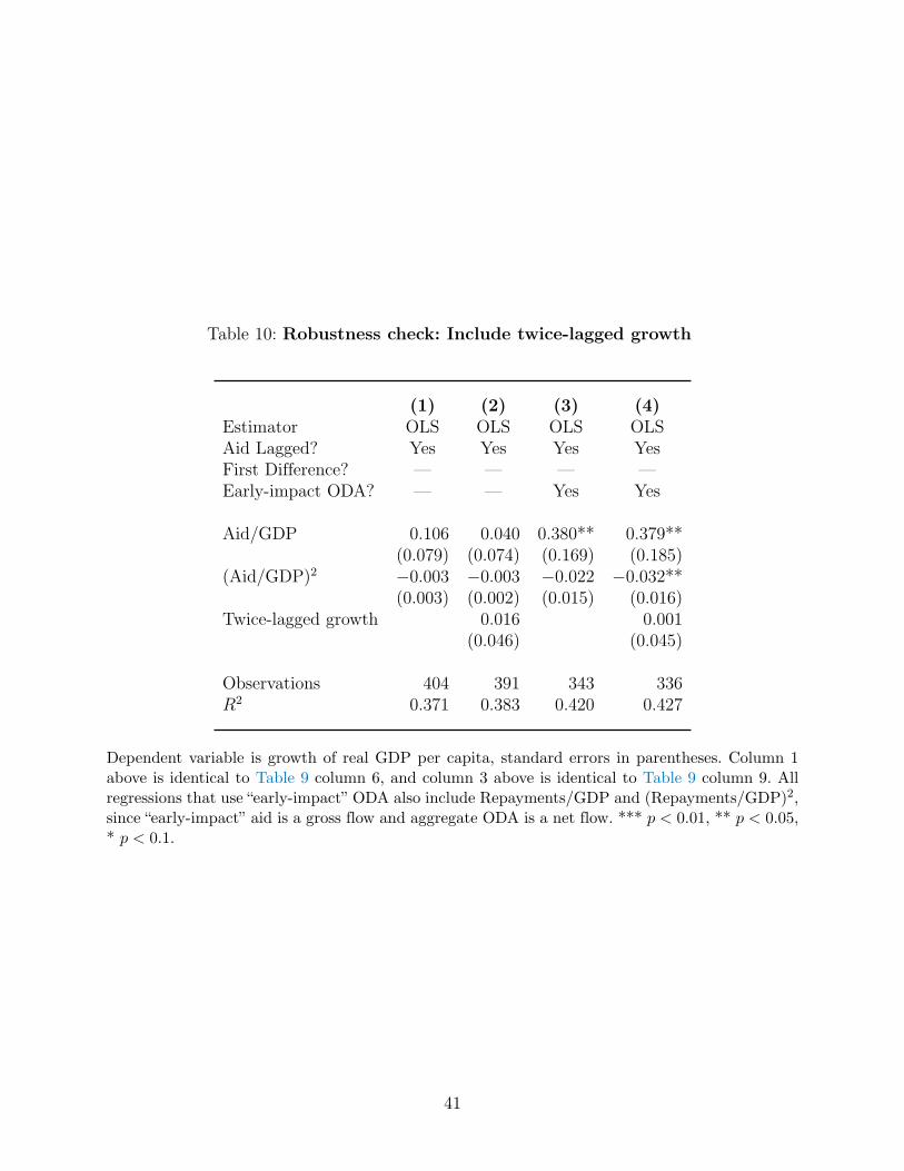
Table 10: Robustness check: Include twice-lagged growth

(1) (2) (3) (4)Estimator OLS OLS OLS OLSAid Lagged? Yes Yes Yes YesFirst Difference? — — — —Early-impact ODA? — — Yes Yes

Aid/GDP 0.106 0.040 0.380** 0.379**(0.079) (0.074) (0.169) (0.185)

(Aid/GDP)2 −0.003 −0.003 −0.022 −0.032**(0.003) (0.002) (0.015) (0.016)

Twice-lagged growth 0.016 0.001(0.046) (0.045)

Observations 404 391 343 336R2 0.371 0.383 0.420 0.427

Dependent variable is growth of real GDP per capita, standard errors in parentheses. Column 1above is identical to Table 9 column 6, and column 3 above is identical to Table 9 column 9. Allregressions that use “early-impact” ODA also include Repayments/GDP and (Repayments/GDP)2,since “early-impact” aid is a gross flow and aggregate ODA is a net flow. *** p < 0.01, ** p < 0.05,* p < 0.1.

41

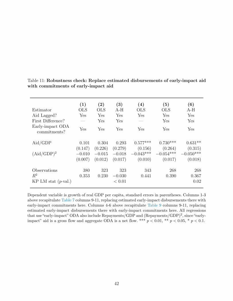
Table 11: Robustness check: Replace estimated disbursements of early-impact aidwith commitments of early-impact aid

(1) (2) (3) (4) (5) (6)Estimator OLS OLS A-H OLS OLS A-HAid Lagged? Yes Yes Yes Yes Yes YesFirst Difference? — Yes Yes — Yes YesEarly-impact ODA

Yes Yes Yes Yes Yes Yescommitments?

Aid/GDP 0.101 0.304 0.293 0.577*** 0.730*** 0.631**(0.147) (0.226) (0.279) (0.156) (0.264) (0.315)

(Aid/GDP)2 −0.010 −0.015 −0.018 −0.043*** −0.054*** −0.050***(0.007) (0.012) (0.017) (0.010) (0.017) (0.018)

Observations 380 323 323 343 268 268R2 0.353 0.230 −0.030 0.441 0.390 0.367KP LM stat (p-val.) < 0.01 0.02

Dependent variable is growth of real GDP per capita, standard errors in parentheses. Columns 1-3above recapitulate Table 7 columns 9-11, replacing estimated early-impact disbursements there withearly-impact commitments here. Columns 4-6 above recapitulate Table 9 columns 9-11, replacingestimated early-impact disbursements there with early-impact commitments here. All regressionsthat use “early-impact” ODA also include Repayments/GDP and (Repayments/GDP)2, since “early-impact” aid is a gross flow and aggregate ODA is a net flow. *** p < 0.01, ** p < 0.05, * p < 0.1.

42

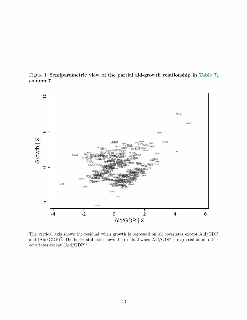
Figure 1: Semiparametric view of the partial aid-growth relationship in Table 7,column 7

ARG3

ARG4

ARG5

ARG6

ARG7

ARG8

ARG9

ARG10

BOL3

BOL4

BOL5

BOL6

BOL7

BOL8

BOL9

BOL10

BRA5

BRA6 BRA7

BRA8

BRA9

BRA10

BWA4

BWA5

BWA6

BWA7

BWA8

BWA9

BWA10CHL3

CHL4

CHL5

CHL6

CHL7

CHL8

CHL9

CHL10

CIV5

CIV6

CIV7

CIV8

CIV9

CIV10

CMR4

CMR5

CMR6 CMR7

CMR8

CMR9

COL3

COL4 COL5

COL6

COL7

COL8

COL9

COL10CRI3

CRI4

CRI5

CRI6

CRI7

CRI8

CRI9

CRI10

DOM3

DOM4

DOM5

DOM6

DOM7

DOM8

DOM9

DOM10 DZA3

DZA9

DZA10

ECU3

ECU4 ECU5

ECU6

ECU7

ECU8

ECU9

ECU10

EGY4

EGY5

EGY6

EGY7

EGY8

EGY9

EGY10

ETH6

ETH7

ETH8

ETH9

GAB3

GAB4

GAB5

GAB6

GAB7GHA3

GHA4 GHA5

GHA6

GHA7

GHA8

GHA9

GMB3

GMB4

GMB5

GMB6

GMB7GTM3

GTM4

GTM5

GTM6

GTM7

GTM8

GTM9

GTM10

HND3

HND4 HND5

HND6

HND7

HND8

HND9

HND10

HTI3

HTI4HTI5

HTI6

HTI7

HTI8

HTI9IDN4

IDN5

IDN6

IDN7

IDN8

IDN9

IDN10

IND3

IND4IND5

IND6

IND7

IND8

IND9

IND10

JAM4JAM5

JAM6

JAM7

JAM8

JAM9

JAM10

KEN3

KEN4

KEN5

KEN6

KEN7

KEN8

KEN9

KEN10

KOR3

KOR4

KOR5

KOR6

KOR7

KOR8LKA3

LKA4

LKA5

LKA6

LKA7

LKA8

LKA9

LKA10

MAR3

MAR4

MAR5

MAR6

MAR7

MAR8

MAR9

MAR10

MDG3

MDG4

MDG5

MDG6

MDG7

MDG8

MDG9MEX3

MEX4

MEX5

MEX6

MEX7MEX8

MEX9

MEX10

MLI7MLI8

MLI9

MLI10

MWI5

MWI6

MWI7

MYS3

MYS4

MYS5

MYS6

MYS7

MYS8

MYS9

NER4

NGA3

NGA4

NGA5

NGA6

NGA7

NGA8

NGA9

NGA10

NIC3

NIC4

NIC5

NIC6

NIC7

NIC8

NIC9

NIC10

PAK3

PAK4

PAK5

PAK6

PAK7

PAK8

PAK9

PAK10

PER3

PER4

PER5

PER6

PER7

PER8

PER9

PER10

PHL3

PHL4 PHL5

PHL6

PHL7

PHL8

PHL9

PHL10

PRY3

PRY4PRY5

PRY6

PRY7

PRY8

PRY9

PRY10

SEN3

SEN4

SEN5

SEN6

SEN7

SEN8

SEN9

SLE3

SLE4

SLE5

SLE6

SLE7

SLE8

SLE9

SLE10

SLV3

SLV4

SLV5

SLV6

SLV7

SLV8

SLV9

SLV10

SYR3

SYR4SYR5

SYR6

SYR7SYR8

SYR9

TGO4

TGO5

TGO6

TGO7

TGO8

TGO9

TGO10

THA3

THA4THA5

THA6

THA7

THA8

THA9

THA10

TTO3

TTO4TTO5

TTO6

TTO7

TTO8TUN6

TUN7TUN8

TUN9

TUN10

TUR3

TUR4

TUR5

TUR6

TUR7

TUR8

TUR9

TZA8

TZA9

TZA10

URY3

URY4URY5

URY6

URY7

URY8

URY9

URY10

VEN3

VEN4

VEN5

VEN6

VEN7

VEN8

VEN9VEN10

ZAR3ZAR4

ZAR5

ZAR6

ZAR7

ZAR8

ZAR9

ZMB7

ZMB8

ZMB9

ZWE5

ZWE6

ZWE7

ZWE8

-50

510

Gro

wth

| X

-4 -2 0 2 4 6

Aid/GDP | X

The vertical axis shows the residual when growth is regressed on all covariates except Aid/GDPand (Aid/GDP)2. The horizontal axis shows the residual when Aid/GDP is regressed on all othercovariates except (Aid/GDP)2.

43