Working Paper 141/14

FAMILY TIES: OCCUPATIONAL RESPONSES TO COPE WITH A HOUSEHOLD INCOME SHOCK

Massimo Baldini Costanza Torricelli

Maria Cesira Urzì Brancati

Family ties: occupational responses to cope with a household income shock

Massimo Baldinia,b, Costanza Torricellia,c,d*, Maria Cesira Urzì Brancatia,d

a. Department Economics, University of Modena and Reggio Emilia

b. CAPP (Centro Analisi Politiche Pubbliche, Modena)

c. CEFIN (Centro Studi di Banca e Finanza, Modena)

d. CeRP (Collegio Carlo Alberto, Torino)

June 2014

Abstract

We use household panel data to explore the link between transitions of a household member (not

only the wife) into the workforce and negative income shocks (unemployment and/or income

support) suffered by another household member. We take the case of Italy where family ties

other than spousal ones are particularly strong, and we also consider the role of household

illiquidity due to housing. After accounting for standard socio-economic controls, results show

significant reactions to income shocks, especially during the Great Recession. Moreover, at high

levels of portfolio illiquidity, transitions are significantly more likely for households hit by a

shock.

JEL: D12; D14; J22; C25

Keywords: household labour decisions; household portfolios; discrete-choice models

* Corresponding author: costanza.torricelli@unimore.it. The authors thank for helpful comments and suggestions Marianna Brunetti, Giuseppe Marotta, and participants to the MAF conference (April 2014) and Netspar conference (June 2014). Usual disclaimers apply.

1

Introduction

During the first year of the Great Recession, between 2008 and 2009, the GDP of the Euro (17)

area dropped by 4.4 per cent according to OECD statistics; in the following months,

unemployment rates soared, especially in Southern European countries (Italy, Spain, Greece and

Portugal), and the value of real and financial assets declined sharply. What began as a financial

crisis sparked by the US housing market bubble (and the abuse of subprime loans) soon turned

into the deepest recession since the 1930s. As a consequence, many households, especially those

who believed the effects of the shocks to be permanent, were forced to reduce consumption

expenditures (Christelis et al. 2012). While different governments in different countries chose

more or less expansionary fiscal and monetary policies to counteract the effect of the crisis, at

the household level individuals adopted a series of strategies to cope with financial strain due to

a loss of income.

From a theoretical point of view, a standard intertemporal budget constraint posits that

individuals facing an unforeseen negative income shock can react in different ways: they may

increase labour supply, reduce planned consumption, resort to borrowing (either from credit

institutions or other family members and friends), or use their savings (Browning and Lusardi,

1996). An increase in labour supply, either at the extensive margin (from not participating in the

labour market to participating) or intensive margin (increasing the number of hours worked)

depends on the relative price and effectiveness of all the alternatives/combinations. As stressed

by Lundberg (1985), when credit constraints are binding and in the absence of savings (or in the

presence of liabilities), increasing labour supply, or at least trying to, is more likely. The recent

increase in the number of active persons in Europe, despite the recession, seems to suggest that

such a reaction could be taking place: data from EUROSTAT show that the active population in

Europe (EU17) has increased by over 2 million units, or 1 per cent, between 2008 and 2013;

however, while the variation in the activity rate is positive for women (+4 per cent, or 2.8 million

units), it has dropped by 1 per cent for men. In Italy, where the drop in GDP has been severe and

potentially more permanent, data from Italian National Institute of Statistics show that among

2

women aged 35-44 years the activity rate from 2008 to 2012 increased from 67.8 per cent to 69

per cent.

The aim of this paper is to analyse the potential increase of labour supply as a coping strategy

against income losses. More specifically, we assess whether inactive individuals (not only the

spouse) who are part of a household hit by an income shock are more likely to transit into the

workforce. By income shock we mean the event that at least one household member (not

necessarily the head of household) fell into unemployment and/or started receiving some kind of

work-related income support, since both cases imply a reduction in family income. Our analyses

are based on a discrete choice model and, besides standard socio-economic and demographic

variables, we use portfolio controls with special attention to portfolio illiquidity due to housing.

We also control for potential sample selection and estimate a standard Heckman selection model.

We use data drawn from the Bank of Italy Survey on Household Income and Wealth (SHIW)

over the period 2004-2012 to include the effects of the Great Recession. Italy lends itself

particularly well to our empirical investigation for three main reasons. First, the role of intra-

family transfers is especially relevant, since “children” live with their parents until well into their

thirties, hence benefiting from (as well as potentially contributing to) parental income and wealth.

The Italian case is not, however, isolated, since the extended co-residence of parents and their

adult children (and/or elderly) is typical of Southern Europe, widespread in most Eastern

European countries, and not negligible in some North-Western countries, such as the UK, Ireland

and Austria (Iacovou and Skew, 2011). Thus, our findings can lead to broader generalisations.

Second, Italians are more able to smooth consumption and less bound by credit constraints

because they are savers (even though the observed level of savings has substantially decreased in

the last decade) and they have very low private debt and a high homeownership rate, therefore

portfolio controls may play an important role. Finally, the low stock market participation of

Italian households (Guiso and Jappelli, 2009) meant that the majority of them were shielded

from huge capital losses due to the financial turmoil (Brandolini et al., 2012), therefore labour

income shocks may have a stronger effect.1

1 It is also worth mentioning that one quarter of total household income comes from pensions and other public transfers which have not been touched by the crisis – except for a two year freeze of indexation for pensions up to

3

Our contribution is twofold. First, we study not just spousal reaction to a household income

shock, but also the reaction of any other household member so as to capture broader family ties

and changes in the family structure. Because of the rigidity of the Italian labour market, we

consider an increase in labour supply at the extensive margin, so our estimation sample consists

only of inactive household members, mainly housewives/ homemakers and students, who may

have an (extra) incentive to participate in the labour market once another household member

experienced an income shock. Since students may enter the labour force independently of the

income shock when they finish studying, besides controlling for age and education, we carry out

a robustness check and split the sample according to the two main inactive categories. Secondly,

among portfolio controls, we specifically account for the role played by portfolio illiquidity due

to housing. We both estimate the impact of portfolio illiquidity itself on the probability of

increasing labour supply, and we assess whether the role of portfolio illiquidity differs between

households hit and those not hit by an income shock.

Our results show a significant positive association between transition probabilities into the

workforce or employment and household income shocks, especially during the recession. The

probability of a transition into employment or into the workforce is concave in age and higher in

the presence of an income shock. As for portfolio controls, we find a significant difference

(mostly in terms of intercept, but also of slope) between the level of illiquidity and labour market

participation for households hit/not hit by a shock.

The rest of the paper is organized as follows. Section 1 provides an overview of the related

empirical and theoretical literature; Section 2 describes the dataset and provides some descriptive

statistics that motivate our research question. Section 3 illustrates the empirical analyses and

discusses results. Sensitivity analyses and robustness checks are presented in Section 4. Last

Section concludes.

1. Literature Review and Conceptual Framework

When studying mechanisms to cope with income drops within a household, it is important to

consider intra-household transfers, which may take the form of monetary transfers as well as

three times the minimum value – therefore families in which an older member is present can benefit from his or her pension (Brandolini et al. 2012).

4

labour supply reactions of another household member. The idea that one inactive household

member may increase his or her labour supply to compensate for the unemployment of another

household member is generally referred to as the “added worker effect”, a concept which dates

as far back as the 1940s (Humphrey, 1940) and has received large attention by the economic

literature. Most authors focus on couples and the wife’s response to husband’s job loss, while

only a few consider the reaction of other members, and the results are still mixed. For instance,

Maloney (1991) finds no evidence of an added worker effect for US couples, since the husband’s

(temporary) unemployment does not lower the wife’s reservation wage. Conversely, Gong

(2010) finds a positive effect of husband’s job loss both on wife’s participation and on working

hours for a sample of Australian women; since it is harder for women who are out of the labour

force to enter the market than for women already working to increase their hours, the study finds

a stronger effect on the intensive margin. Bryan and Longhi (2013) find little evidence in support

of a “household insurance” mechanism for British couples in case of unpredicted job loss. More

specifically, the authors compare booms and recession periods and find that, even though job

searches increase in response to job loss during a recession, they are not necessarily successful.

Household members’ reactions likely depend on the level and availability of public transfers.

Cullen and Gruber (2000) and Bingley and Walker (2001) highlight the importance of

unemployment insurance and the incentives embedded in the system. Using US data, Cullen and

Gruber estimate that spouses would increase their total hours of work by 30 per cent in response

to an income shock if unemployment insurance did not exist. Bingley and Walker use UK data to

exploit the 1996 welfare reform, which replaced the existing system of unemployment benefits

with the Job Seeker’s Allowance, and found similar effects. A couple of studies, Skoufias and

Parker (2005) and Beylis (2012), deal with similar issues using Mexican data. The authors claim

that because in Mexico, like in other developing countries, labour markets are still hierarchical in

terms of gender with married women often seen as secondary workers, the access to credit is

poor, and unemployment insurance is non-existent, wives are more likely to increase their labour

supply in response to their husbands’ job loss; indeed, both articles find a large and significant

added worker effect. Benito and Saleheen (2012) consider the impact of a financial rather than

income shock and find a positive response in terms of labour supply, mainly at the intensive

margin, for a sample of British households.

5

Portfolio features may well play a role in determining labour transitions. Blundell et al. (1997)

give the theoretical background to relate wealth and labour market transitions positing that a

higher level of wealth decreases the probability of a transition from non-employment into

employment. Bloemen (2002) presents an empirical study for the Netherlands on the relation

between wealth and labour market transitions, where to define wealth he uses the levels of net

assets, and finds a negative relationship between wealth at the beginning of the period and the

probability to remain employed/transit into employment. Another strand of literature looks at the

connection between mortgage commitments and female labour supply (e.g. Del Boca and

Lusardi, 2003 and Fortin, 1995) and finds a positive relationship.

A few recent studies, which fit within the literature on household financial fragility, investigate

the role of portfolio composition and intra-family monetary transfers in determining the ability to

cope with financial shocks that may be due to temporary and unexpected income drops. Lusardi

et al (2011) use a self-assessed measure of financial fragility and study US households’ ability to

come up with $2,000 in 30 days, compare their coping ability with that of households in seven

other industrialized countries and also look at a “pecking order” of coping mechanisms (savings,

family/friends, traditional credit, work more, selling possession). Brunetti et al. (2012) propose a

novel characterization of financial fragility that is not necessarily linked to indebtedness and is

free of subjectivity bias and use it to assess the importance of household portfolio illiquidity in

determining difficulties to cope with unexpected expenditure needs, thereby including temporary

income losses.

With respect to the literature on the “added worker effect”, we study not just spousal reaction to

a household income shock, but the reaction of any other household member so as to capture

broader family ties and changes in the family structure, which are happening in many European

countries. Indeed, the share of young adults, 18 to 34 year olds, living with their parents has been

steadily increasing not just in Southern Europe, but also in several European countries where

traditionally children gain their independence at younger ages (i.e. the UK, France or the

Netherlands2); hence we may look for an added worker effect also among older children. With

respect to the literature on wealth and labour transitions, we account for portfolio composition

2 Source: EU-SILC; EUROSTAT data.

6

and, specifically, we control for the role played by portfolio illiquidity due to housing, in line

with some of the literature on household financial fragility.

2. Data and Descriptive Statistics

2.1 Sample Selection and descriptive statistics

Our investigation draws from the Survey on Household Income and Wealth (SHIW) waves

2004-2012. The SHIW is a biannual survey, conducted by the Bank of Italy on a representative

sample of the Italian population and includes a wealth of information on socio-demographic

variables, a detailed description of households’ assets and work histories. We kept only

individuals present in at least two waves, so that we can exploit the panel component, and we

restrict our sample to individuals aged between 15 and 65; however, we control for the presence

of children under the age of five within the household, as well as for the presence of adults aged

65 and over.

In this Section we present a few descriptive statistics of household income, first at an aggregate

level and then distinguishing between households hit and not hit by an income shock as defined

below.

2.2 Changes in total household income and its components

In order to understand the income dynamics during the period considered, we first calculate the

mean level of total household disposable income and its separate components for each wave. All

income definitions are given in Appendix A.

From table 1 we notice how payroll and pension income follow the same trend as total household

disposable income, peaking in 2008, experiencing a large drop in 2010 and then decreasing again,

but less than in the previous period 3 . Conversely, income from self-employment shows a

decreasing trend from the beginning of the period in 2004 till 2012. Transfer income is

decreasing before 2008, and increasing right after, which can be seen as a sign of the economic

crisis. Property income and income from financial assets show an unstable trend. Property

3 Please note that our sample does not include people aged over 65, so the variation in pension income is not meant to be representative for the entire Italian population.

7

income appears to represent a high portion of total household disposable income, but it has to be

recalled that it consists of two components: while actual rents increase in the last biennium,

imputed rents decline markedly between 2010 and 2012, possibly reflecting people’s negative

expectations on the housing market. Income from financial assets in 2010 is shown as negative

because interests paid, most likely on mortgages, are higher than interests earned.

In table 2 we show the wave-on-wave variation of the income variables to highlight the potential

impact of the recession. Indeed, between 2008 and 2010 we observe the first and largest drop in

both payroll income and total household disposable income (-5.9 per cent and -5.4 per cent

respectively), and the negative trend continues into the following biennium (-1.7 per cent and -

2.4 per cent respectively). Between 2010 and 2012 payroll income decreases less than total

household disposable income, possibly reflecting the large negative variation in income from

self-employment (-12.2 per cent).

Table 1: Aggregate household income and its components (CPI adjusted 2012 prices, in €)

€ 2004 2006 2008 2010 2012 Payroll Income 19,941 21,068 21,344 20,077 19,740 Self-employment Income 6,515 6,493 6,219 6,030 5,463

Self-employment Income 5,623 5,702 5,424 5,328 4,676 Entrepreneurial Income 892 791 795 703 787

Pension Income 4,508 4,601 5,199 4,527 4,462 Pensions 4,493 4,532 5,158 4,515 4,439 Arrears 16 69 41 12 23

Transfer Income(a) 223 199 179 267 424 Property Income 7,547 7,236 7,378 7,587 7,012

Actual Rents 502 307 346 384 400 Imputed Rents 7,044 6,929 7,032 7,203 6,611

Income from Financial Assets -30 108 -44 -327 45 Total Household Disposable Income 38,832 39,712 40,308 38,130 37,203 Obs 6,305 8,227 8,682 8,714 6,818 (a) We have not reported the sub-categories gifts, alimonies and other transfers.

Source: SHIW 2004-2012, data weighted using household sampling weights.

8

Table 2: Percentage change in aggregate household income and its components

(CPI adjusted 2012 prices)

2004-2006 2006-2008 2008-2010 2010-2012Delta Payroll Income 5.7% 1.3% -5.9% -1.7% Delta Self-employment Income -0.4% -4.2% -3.0% -9.4%

Self-employment Income 1.4% -4.9% -1.8% -12.2% Entrepreneurial Income -11.3% 0.6% -11.6% 12.0%

Delta Pension Income 2.1% 13.0% -12.9% -1.4% Pensions 0.9% 13.8% -12.5% -1.7% Arrears 343.6% -40.7% -70.5% 89.7%

Delta Transfer Income(a) -11.0% -9.9% 48.8% 59.0% Delta Property Income -4.1% 2.0% 2.8% -7.6%

Actual Rents -38.8% 12.5% 11.0% 4.3% Imputed Rents -1.6% 1.5% 2.4% -8.2%

Delta Income from Financial Assets(b) -459.1% -140.8% 642.6% -113.8% Delta Total Household Disposable Income 2.3% 1.5% -5.4% -2.4% Obs(c) 6,208 6,691 6,875 6,802 (a) We have not reported the sub-categories gifts, alimonies and other transfers.

Note: Since we are calculating variations, observations from the first year are missing. All delta variables are calculated as the % variation from the previous wave (xt-xt-1)/xt-1. Source: SHIW 2004-2012, data weighted using household sampling weights.

Aggregate measures, however, do not take into account an important source of heterogeneity:

some households experienced an income shock and some did not. Therefore, we want to see to

what extent the variation in household income follows a different pattern for the two groups.

2.3 Defining households hit by an income shock

In order to identify households hit by an income shock, we build a binary variable equal to one if

at least one household member transited from employment into unemployment, at least one

household member started receiving some kind of income support (income from redundancy

benefits, mobility benefits and unemployment benefits) or both, and zero otherwise. We consider

the receipt of work-related benefits as an income shock, since in Italy many workers of firms

suffering from severe reductions in their activity receive redundancy or mobility benefits, but are

still classified as employed, even though the probability of working again may be low. Because

redundancy/mobility benefits cover only a percentage of the initial wage, family income is

reduced and therefore other family members may react by searching for a job.

9

Between 2012 and 2010, 11.7 per cent of the families in our sample were hit by a shock

compared to 4.9 per cent in 2004-2006. More specifically, a transition from employment into

unemployment is present in roughly 7.2 per cent of families in 2012, compared to 4.4 per in

2004-2006; while 6.2 per cent of families in 2012 report at least one member who started

receiving benefits, as opposed to 1.2 per cent in 2004-2006 (see table 3). The categories do not

totally overlap, since we have households in which only one of the two shocks (unemployment

or benefits) is presents, and households in which both of them are present at the same time.

Table 3: Individuals living in households which experienced / did not experience an income shock, by year 2004-2006 2006-2008 2008-2010 2010-2012 Income shock (composite) between t and t-1

4.9% 6.1% 5.8% 11.7%

Only one shock: lost work 4.4% 4.7% 3.3% 7.2% Only one shock: benefits 1.2% 1.9% 3.2% 6.2%

Obs 7,650 8,262 8,292 6,361 Source: SHIW 2004-2012, data weighted using household sampling weights. Figure 1 shows the average income variation for households hit and not hit by an income shock.

Predictably, payroll and self-employment income show large negative variations in all periods

for households hit by a shock (except for a small positive variation in self-employment income

between 2008 and 2010), while the variation in transfer income for this group is always positive.

Since the beginning of the recession the variation in payroll and self-employment income

becomes negative, albeit small, also for households not hit by an income shock.

10

Figure 1: Variation in household income components (in CPI adjusted euros, by wave and income shock)

1 Only wage, no fringe benefits. 2 Only pensions, no arrears 3 Only financial assistance (no gifts or alimonies) Source: Our elaborations from SHIW 2004-2012.

One of the intuitions we draw from Figure 1 is that the severe loss in payroll income for

households hit by a shock is far from being compensated by an equivalent increase in other types

of income, especially transfer income. It is therefore plausible to expect, among reactions at the

household level, an increase in the labour supply.

3. Empirical Strategy

Since we are interested in the reaction to a household income shock from previously inactive

household members, we start by defining who is considered inactive. We build a binary variable

equal to 1 if the individual was a housewife/homemaker, a student, a voluntary worker or if he or

she lived of independent means (i.e. rentier) when he or she first enters our sample. Pensioners or

recipients of non-work-related benefits are excluded. Since we have an unbalanced panel, the

first year does not correspond to 2004, but can be any successive year.4 As we can see in table 4,

roughly 52.2 per cent of the people who were inactive at time 1 were students, 47.3 per cent were

4 A technical note: the first year of inactivity cannot be 2012 because in that case the individual would only be present for one period and would be dropped from our estimation sample.

11

housewives and only 0.5 per cent were either rentiers or voluntary workers. Given these numbers,

we carry out a robustness check on the two categories housewives and students in Section 4.

We then define the dependent variable Employedit as a dichotomous variable taking the value of

1 if the individual i transited from out of the workforce into employment at time t and zero

otherwise; if at time t+1, the individual who experienced the transition remains in employment,

the binary variable takes the value of 1. If the same individual transits out of employment (at t+1),

the binary variable takes the value of zero. This gives us a total of 986 observations (for 587

individuals). Because a transition into employment is likely to be more difficult during a

recession, we also define a second dependent variable, Activeit, as a dichotomous variable taking

the value of 1 if the individual transited from out of the workforce into the workforce (i.e. either

employed or actively seeking work) at time t or if he or she remained part of the workforce after

a transition, and zero otherwise, for a total of 2,005 observations (for 1,162 individuals).

Even though the percentage of women who are inactive in the first year is 2.7 times higher than

the percentage of men in the same situation (73 per cent vs. 27 per cent), only 14 per cent of

these women experience a transition into the workforce as opposed to 25 per cent of men (see

Table 4).

Table 4: Estimation sample and employment transitions, by gender

Male Female All % of Obs Indiv. Obs Indiv. Obs Indiv. Female

out of All Inactive at t= 1 2,041 951 5,584 2,556 7,625 3,507 73%

of which students 2,009 937 1,953 948 3,962 1,885 49% of which housewives 4 2 3,618 1,603 3,622 1,605 100% of which voluntary workers 23 10 10 4 33 14 30% of which rentiers 5 2 3 1 8 3 38%

Transited into employment 411 238 575 349 986 587 58% Transited into workforce 878 476 1,127 686 2,005 1,162 56% Remained inactive 1,123 685 4,260 2,180 5,383 2,865 79% Success rate into employment 25% 14% Success rate into workforce 50% 27% Source: Own elaborations from SHIW data. Note: totals do not add up since the same individual may experience more than one transition. For instance, the same individual can start out of the workforce, remain out for a year, and then transit into the workforce/employment.

12

We estimate the following equation as a static probit model:

{ }|1|01 11 =≥++= iitijtijtit InactivexkIncomeShocy εγβ (1.1)

where

yit is Employedit in a first specification, or Activeit in a second specification; Income shockijt=1 if

the individual i is part of a household j in which at least one member has suffered an income

shock (either became unemployed or received income support or both) from time t onwards; xit is

a vector of covariates to control for heterogeneity; εit the error, which we assume to be normally

distributed, and inactivei1=1 if individual i at time 1 is inactive.

The vector of covariates x includes a dummy variable equal to one if the individual is a female, a

second order polynomial in age, dummies for marital status (couple as the baseline), a dummy

for the presence of children under the age of 5 within the household and one for the presence of

an individual aged 65 and over, household size, dummy for head of household, dummies for high

and medium educational attainment (low education as the baseline), year and geographical

dummies. A detailed list of all variables used, their definition and summary statistics of the

estimation sample are provided in Appendix B.

Since we are using a panel, our sample contains several observations on the same individuals

which are not independent of each other. We control for it by clustering standard errors at the

individual level.

3.1 The role of income shocks

Table 5 highlights the role of an income shock and reports the results from regression (1.1) in the

two specifications, whereby in the first the dependent variable is the probability of becoming

employed and in the second the probability of becoming active.5

5 Since our regressor of interest, Income Shock, is a binary variable, interpreting the marginal effects (at means) is straightforward: the coefficient is just the difference between the predicted probabilities of a transition, conditional on other covariates, for households hit by a shock and households not hit by a shock, holding all other variables at their means. So the MEM for Yshock = Pr(Y = 1|X, Yshock = 1) – Pr(y=1|X, Yshock = 0).

13

These results confirm our intuition that households hit by a shock respond by increasing labour

supply, as the probability of a transition is 7.7 percentage points higher compared to households

that were not hit by an income shock. The effect is even stronger if we consider the probability

of a transition into the workforce, with individuals living in a household hit by an income shock

9.3 percentage points more likely to become active than individuals living in households in

which nobody suffered an income shock. Despite the fact that most individuals who transit from

inactivity into either employment or the workforce are women, their relative success rate - as

measured by the percentage of women who experience a transition over total women out of the

workforce - compared to men is much lower (Table 4), therefore it is not surprising to find a

negative sign on the marginal effect for the female dummy. From Table 5, we also see that the

probability of a transition increases with age (in a concave fashion) and is higher for people who

are not married. It is also significantly increasing with years of education (at the same age) and

for those who live in the Northern area of Italy, where the number of job opportunities is greater.

14

Table 5: Probability of a transition from out of the workforce into the workforce Pr(Y=1) Y=1: Employed Y=1: Active Coeff MEMs Coeff Y* MEMs Income shock 0.240*** 0.077*** 0.235*** 0.093*** (0.07) (0.02) (0.06) (0.02) Demographics Female -0.316*** -0.095*** -0.321*** -0.127*** (0.07) (0.02) (0.06) (0.02) Age 0.180*** 0.009*** 0.201*** 0.009*** (0.02) (0.00) (0.02) (0.00) Age squared(a) -0.002*** -0.003*** (0.00) (0.00) Single 0.696*** 0.203*** 1.029*** 0.386*** (0.14) (0.04) (0.13) (0.05) Divorced 0.454* 0.121 0.938*** 0.351*** (0.24) (0.08) (0.21) (0.08) Widow(er) 0.478 0.128 0.786** 0.291** (0.38) (0.12) (0.32) (0.13) With children aged <5 in HH 0.023 0.007 -0.092 -0.036 (0.12) (0.04) (0.10) (0.04) At least one over 65 in HH -0.049 -0.015 0.142* 0.056* (0.09) (0.03) (0.07) (0.03) Household size -0.054* -0.016* -0.020 -0.008 (0.03) (0.01) (0.02) (0.01) Head 0.175** 0.053** 0.108 0.043 (0.08) (0.03) (0.07) (0.03) Graduate 0.296*** 0.089*** 0.514*** 0.203*** (0.10) (0.03) (0.09) (0.03) Secondary Education 0.229*** 0.069*** 0.222*** 0.088*** (0.07) (0.02) (0.06) (0.02) Resident in the Centre -0.171** -0.060** 0.050 0.020 (0.08) (0.03) (0.07) (0.03) Resident in the South -0.589*** -0.179*** -0.094* -0.037* (0.06) (0.02) (0.05) (0.02) Cons -4.278*** -4.700*** (0.39) (0.35) Year YES YES # observations 7,822 7,822 # individuals 3,582 3,582 Pseudo R2 0.120 0.173 P value 0.000 0.000 χ2 321.87 816.96

Clustered robust standard errors in parentheses; * p<0.01, ** p<0.005, *** p<0.001 The marginal effects (MEMs) are calculated at the average values of the covariates in the sample. (a) The marginal effect of Age includes the effect of age squared.

3.2 The role of income shocks at different ages

In order to better understand the role of age in explaining transitions into employment or into the

workforce in the presence of a family income shock, we look at interactions. Because we are

15

estimating a nonlinear model, the best way to represent the effect of income shock and age is to

show the marginal effects at representative values (of age). Table 6 shows that the income shock

induces a change in labour supply also for middle ages, and not only for the younger people (e.g.

students), who might have natural transitions into the workforce when they finish their studies.

However, while in the case of the transition into employment the effect of the shock is

significant for all age classes until 53 years, when looking at transitions to the workforce, it

ceases to be relevant some years earlier.

Table 6: Probability of a transition from out of the workforce into workforce interacting income shock and age

Marginal effect of income shock at representative ages Pr(Y=1) Y=1: Employed Y=1: Active Income Shock at age 17 0.019* 0.079*** (0.01) (0.02) Income Shock at age 23 0.044** 0.112*** (0.02) (0.03) Income Shock at age 29 0.066*** 0.106*** (0.02) (0.03) Income Shock at age 35 0.076*** 0.079*** (0.03) (0.03) Income Shock at age 41 0.075*** 0.049* (0.03) (0.03) Income Shock at age 47 0.068** 0.018 (0.04) (0.03) Income Shock at age 53 0.054 -0.011 (0.04) (0.04) Income Shock at age 59 0.035 -0.024 (0.03) (0.03) Income Shock at age 65 0.015 -0.015 (0.02) (0.01) Year YES YES Demographics YES YES # observations 7,822 7,626 # individuals 3,582 3,507 The marginal effects (MEMs) are calculated at the average values of the covariates in the sample. All models include the following controls: dummy variable equal to one if the individual is a female, a second order polynomial in age, dummies for marital status (couple as the baseline), a dummy for the presence of children under the age of 5 within the household, a dummy for the presence of an adult aged 65 or over in the household, household size, dummy for head of household, dummies for high and medium educational attainment (low education as the baseline), year and geographical dummies.

16

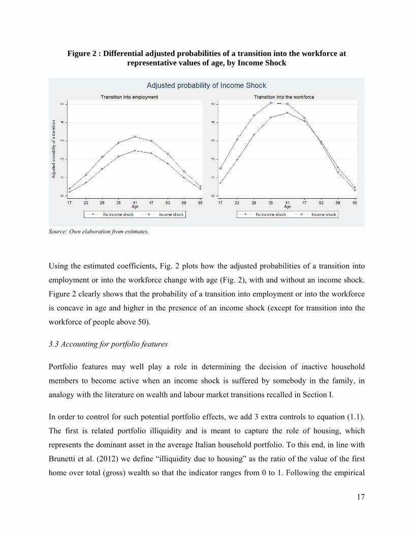
Figure 2 : Differential adjusted probabilities of a transition into the workforce at representative values of age, by Income Shock

Source: Own elaboration from estimates.

Using the estimated coefficients, Fig. 2 plots how the adjusted probabilities of a transition into

employment or into the workforce change with age (Fig. 2), with and without an income shock.

Figure 2 clearly shows that the probability of a transition into employment or into the workforce

is concave in age and higher in the presence of an income shock (except for transition into the

workforce of people above 50).

3.3 Accounting for portfolio features

Portfolio features may well play a role in determining the decision of inactive household

members to become active when an income shock is suffered by somebody in the family, in

analogy with the literature on wealth and labour market transitions recalled in Section I.

In order to control for such potential portfolio effects, we add 3 extra controls to equation (1.1).

The first is related portfolio illiquidity and is meant to capture the role of housing, which

represents the dominant asset in the average Italian household portfolio. To this end, in line with

Brunetti et al. (2012) we define “illiquidity due to housing” as the ratio of the value of the first

home over total (gross) wealth so that the indicator ranges from 0 to 1. Following the empirical

17

literature on wealth and labour transitions, we control for the amount of financial assets and

liabilities measured in 10,000 euros. Financial assets include deposits, government and other

securities and trade credits or credit due from other households; financial liabilities include

liabilities to banks and financial companies (incl. mortgages), trade debt and debts towards other

households.

We then estimate the following equation:

{ }|1|01 111 =≥+++= − iitjtijtijtit inactiveWxkIncomeShocy ελγβ (1.2)

where yit, Income shockijt, xit are the variables we have already specified, and Wjt is a vector of

portfolio controls lagged by one period, including the illiquidity index. Note that portfolio

controls are at household and not individual level.

Table 7 (second and fourth columns) shows that even after including portfolio controls the

results remain stable, since individuals living in a household hit by a shock are still significantly

more likely to transit both into employment (+8.5 ppts) and into the workforce (+9.1ppts). If we

focus on the direct effect of portfolio controls, we see that they are not significant in explaining

transition into employment, but they are relevant in explaining the decision to become active. As

expected, the level of financial assets in the previous period reduces the probability of entering

the workforce, which is consistent with the literature on wealth and labour market transitions

(Blundell et. al, 1997; Stancanelli, 1999; Bloemen, 2002). The negative sign of the coefficient of

the degree of illiquidity due to housing could be explained in principle by two main reasons, both

discouraging participation: housing provides income or collateral for consumer credit (Benito,

2009) and/or owning a house hinders job mobility (see Battu et al. 2008).

18

Table 7: Probability of a transition from out of the workforce into the workforce with portfolio controls

Pr(Y=1) Y=1: Employed Y=1: Active MEMs MEMs MEMs MEMs Income shock 0.077*** 0.085*** 0.093*** 0.091*** (0.02) (0.02) (0.02) (0.02) Demographics Female -0.095*** -0.095*** -0.127*** -0.122*** (0.02) (0.02) (0.02) (0.02) Age / Age squared(a) 0.009*** 0.009*** 0.009*** 0.010*** (0.00) (0.00) (0.00) (0.00) Single 0.203*** 0.199*** 0.386*** 0.397*** (0.04) (0.04) (0.05) (0.05) Divorced 0.121 0.115 0.351*** 0.302*** (0.08) (0.08) (0.08) (0.09) Widow(er) 0.128 0.105 0.291** 0.245 (0.12) (0.14) (0.13) (0.15) With children aged <5 in HH 0.007 0.012 -0.036 -0.029 (0.04) (0.04) (0.04) (0.04) At least one over 65 in HH -0.015 -0.015 0.056* 0.058* (0.03) (0.03) (0.03) (0.03) Household size -0.016* -0.016* -0.008 -0.006 (0.01) (0.01) (0.01) (0.01) Head 0.053** 0.057** 0.043 0.048* (0.03) (0.03) (0.03) (0.03) Graduate 0.089*** 0.091*** 0.203*** 0.213*** (0.03) (0.03) (0.03) (0.04) Secondary Education 0.069*** 0.070*** 0.088*** 0.093*** (0.02) (0.02) (0.02) (0.02) Resident in the Centre -0.060** -0.057** 0.020 0.019 (0.03) (0.03) (0.03) (0.03) Resident in the South -0.179*** -0.173*** -0.037* -0.045** (0.02) (0.02) (0.02) (0.02) Wealth Illiquidity due to housing at t-1 - -0.021 - -0.050** - (0.02) - (0.02) Financial assets (in 10,000€) at t-1 - 0.000 - -0.003** - (0.00) - (0.00) Financial liabilities (in 10,000€) at t-1 - 0.003 - 0.000 - (0.00) - (0.00) Year YES YES YES # observations 7,822 7,625 7,822 7,625 # individuals 3,582 3,507 3,582 3,507 Pseudo R2 0.120 0.120 0.173 0.175 P value 0.000 0.000 0.000 0.000 χ2 321.87 322.54 816.96 799.65

Clustered robust standard errors in parentheses; * p<0.01, ** p<0.005, *** p<0.001 The marginal effects (MEMs) are calculated at the average values of the covariates in the sample. (a) The marginal effect of Age includes the effect of age squared.

19

Since portfolio illiquidity may have a differential effect for households hit/not hit by a shock, we

also look at interactions. Table 8 indicates that portfolio illiquidity due to housing plays a role in

connection with the income shocks. The intensity of the reaction increases, although mildly, with

illiquidity, and more significantly so for people looking for a job. While there is no significant

difference at very low illiquidity levels between households hit/not hit by a shock, at higher

levels of illiquidity (from 0.2 onwards) households hit by a shock are significantly more likely to

transit into employment or into the workforce compared with households in which nobody

experienced an income shock. The result is consistent with the literature on household financial

fragility: Brunetti et al. (2012) stress portfolio illiquidity due to excessive housing as a source of

financial fragility for Italian households.

The coefficients for the adjusted predicted probabilities are plotted in Figure 3. We see that,

although small, the degree of illiquidity due to housing makes a difference. For individuals living

in households not hit by an income shock, the association between illiquidity and the probability

of any occupational transition is negative. By contrast, for the other group of individuals,

illiquidity does not appear to really matter for transitions into the workforce, while it is mildly

but positively associated with the probability of transition into employment. Hence, for people

hit by a household income shock, it seems that the effects of housing mentioned above (i.e.

collateral for consumer credit as in Benito (2009) or discouraging mobility as in Battu et al.,

2008) do not apply.

20

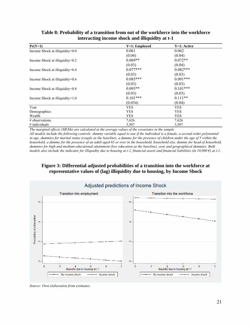
Table 8: Probability of a transition from out of the workforce into the workforce interacting income shock and illiquidity at t-1

Pr(Y=1) Y=1: Employed Y=1: Active Income Shock at illiquidity=0.0 0.061 0.062 (0.04) (0.04) Income Shock at illiquidity=0.2 0.069** 0.072** (0.03) (0.04) Income Shock at illiquidity=0.4 0.077*** 0.082*** (0.03) (0.03) Income Shock at illiquidity=0.6 0.085*** 0.091*** (0.03) (0.03) Income Shock at illiquidity=0.8 0.093** 0.101*** (0.03) (0.03) Income Shock at illiquidity=1.0 0.101*** 0.111** (0.034) (0.04) Year YES YES Demographics YES YES Wealth YES YES # observations 7,626 7,626 # individuals 3,507 3,507 The marginal effects (MEMs) are calculated at the average values of the covariates in the sample. All models include the following controls: dummy variable equal to one if the individual is a female, a second order polynomial in age, dummies for marital status (couple as the baseline), a dummy for the presence of children under the age of 5 within the household, a dummy for the presence of an adult aged 65 or over in the household, household size, dummy for head of household, dummies for high and medium educational attainment (low education as the baseline), year and geographical dummies. Both models also include the indicator for illiquidity due to housing at t-1, financial assets and financial liabilities (in 10,000 €) at t-1.

Figure 3: Differential adjusted probabilities of a transition into the workforce at representative values of (lag) illiquidity due to housing, by Income Shock

Source: Own elaboration from estimates.

21

3.4 Potential sample selection bias

For our estimation strategy, we kept only individuals who were inactive at time 1, therefore

excluding from our sample all individuals who actively looked for a job, as well as those who

were at some time employed and subsequently left the workforce. For this reason, we are dealing

with a non-randomly selected sample, and we may have reasons to believe that some

unobservable characteristics may be correlated with both selection into the estimation sample

and the probability of a transition. We thus check for sample selection bias and estimate a

standard Heckman selection model (Heckman, 1979) by maximum likelihood. The uncensored

sample consists of 23,711 observations for 11,399 individuals.

Our outcome equation is:

{ }01 11 ≥+++= − itjtijtijtit WxkIncomeShocy ελγβ (1.3)

While our selection equation is:

{ }01 111 >++++= − itijtjtijtijti uzWxkIncomeShocInactive ωλγβ (1.4)

where εit and uit are assumed to have a bivariate normal distribution with zero means and

correlation ρ. The vector of covariates for the selection equation includes the same regressors

present in the equation (1.3), plus an excluded variable that determines selection, but has no

direct effect on yit so as to avoid collinearity. The excluded variable zijt is a dummy equal to 1 if

the head of household’ mother was working when she was the same age as the head of household.

The choice of such variable is consistent with both literature on parental attitudes, learning and

beliefs formation (Farré and Vella, 2013; Fogli and Veldkamp, 2011; Fortin, 2005) and literature

on intergenerational income mobility and correlation in unemployment (Björklund and Jäntti,

2012; Ekhaugen, 2009).

In table 9 we report the marginal effects for the outcome equation conditional on selection6

(columns 2 and 4), as well as the marginal predicted probability of selection (columns 3 and 6).

6 Pr(yit=1 | Inactivei1=1) = Pr(yit=1, Inactivei1=1)/Pr(Inactivei1=1).

22

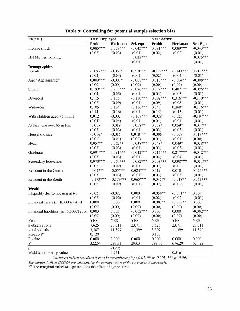
Table 9: Controlling for potential sample selection bias Pr(Y=1) Y=1: Employed Y=1: Active Probit Heckman Sel. eqn Probit Heckman Sel. Eqn Income shock 0.085*** 0.079*** -0.043*** 0.091*** 0.089*** -0.043*** (0.02) (0.03) (0.01) (0.02) (0.02) (0.01) HH Mother working -0.023*** -0.025*** (0.01) (0.01) Demographics Female -0.095*** -0.067* 0.218*** -0.122*** -0.141*** 0.219*** (0.02) (0.04) (0.01) (0.02) (0.04) (0.01) Age / Age squared(a) 0.009*** -0.001* -0.008*** 0.010*** -0.004** -0.008*** (0.00) (0.00) (0.00) (0.00) (0.00) (0.00) Single 0.199*** 0.233*** -0.096*** 0.397*** 0.407*** -0.096*** (0.04) (0.05) (0.01) (0.05) (0.05) (0.01) Divorced 0.115 0.135 -0.110*** 0.302*** 0.316*** -0.110*** (0.08) (0.09) (0.01) (0.09) (0.08) (0.01) Widow(er) 0.105 0.124 -0.116*** 0.245 0.268* -0.116*** (0.14) (0.16) (0.01) (0.15) (0.15) (0.01) With children aged <5 in HH 0.012 -0.002 -0.107*** -0.029 -0.023 -0.107*** (0.04) (0.04) (0.01) (0.04) (0.04) (0.01) At least one over 65 in HH -0.015 -0.019 -0.018** 0.058* 0.059* -0.017** (0.03) (0.03) (0.01) (0.03) (0.03) (0.01) Household size -0.016* -0.015 0.018*** -0.006 -0.007 0.018*** (0.01) (0.01) (0.00) (0.01) (0.01) (0.00) Head 0.057** 0.062** -0.038*** 0.048* 0.049* -0.038*** (0.03) (0.03) (0.01) (0.03) (0.03) (0.01) Graduate 0.091*** 0.091*** -0.042*** 0.213*** 0.217*** -0.042*** (0.03) (0.03) (0.01) (0.04) (0.04) (0.01) Secondary Education 0.070*** 0.069*** -0.052*** 0.093*** 0.098*** -0.051*** (0.02) (0.02) (0.01) (0.02) (0.02) (0.01) Resident in the Centre -0.057** -0.057** 0.024*** 0.019 0.018 0.024*** (0.03) (0.03) (0.01) (0.03) (0.03) (0.01) Resident in the South -0.173*** -0.179*** 0.065*** -0.045** -0.048** 0.065*** (0.02) (0.02) (0.01) (0.02) (0.02) (0.01) Wealth Illiquidity due to housing at t-1 -0.021 -0.023 0.009 -0.050** -0.051** 0.009 (0.02) (0.02) (0.01) (0.02) (0.02) (0.01) Financial assets (in 10,000€) at t-1 0.000 0.000 0.000 -0.003** -0.003** 0.000 (0.00) (0.00) (0.00) (0.00) (0.00) (0.00) Financial liabilities (in 10,000€) at t-1 0.003 0.003 -0.002*** 0.000 0.000 -0.002*** (0.00) (0.00) (0.00) (0.00) (0.00) (0.00) Year YES YES YES YES YES YES # observations 7,625 23,711 23,711 7,625 23,711 23,711 # individuals 3,507 11,399 11,399 3,507 11,399 11,399 Pseudo R2 0.120 0.175 P value 0.000 0.000 0.000 0.000 0.000 0.000 χ2 322.54 293.31 293.31 799.65 676.29 676.29 ρ -0.295 Wald test (ρ=0) - p value 0.251 0.516

Clustered robust standard errors in parentheses; * p<0.01, ** p<0.005, *** p<0.001 The marginal effects (MEMs) are calculated at the average values of the covariates in the sample. (a) The marginal effect of Age includes the effect of age squared.

23

The sign, magnitude and statistical significance of all coefficients in the outcome equation,

including the one on income shock, are essentially the same as in the pooled probit regressions.

Quite interestingly, the only coefficient which loses statistical significance is the one on the

female dummy. However, the Wald test for independent equations tells us that the selection

mechanism is ignorable, as we cannot reject the null hypothesis of independent equations (χ2:

1.32; p-value: 0.251 and χ2: 0.42; p-value: 0.516). As a consequence, we can consider the pooled

probit results in column 1 and 3 as our benchmark estimates.

4. Sensitivity analyses and robustness checks

Three are the main types of sensitivity and robustness checks we consider important for our

investigation.

First of all, since our investigation period covers both a normal cycle phase and a recessionary

one, we want to see whether the results change across these two different periods. To this end,

we run regressions over the 2004-2008 and 2008-2012 separately. Results in Table 10 show that

the sensitivity of labour supply to the labour conditions of other family members is actually

strongly increased in the period of the recession which started in 2008. Indeed, in the first period

there is low to no significant effect of an income shock on labour supply before 2008, while the

other independent variables keep the same signs already found in Tab. 6. Why such a change in

the reaction to an income shock? Before the crisis, the job loss by a family member could be

considered as a transitory phenomenon that soon could be reversed, but with the strong increase

in the unemployment rate, the probability of finding a new job after losing one is lower, and this

pushes other family members to look for a job, so as to increase the joint probability of obtaining

income from work for the family as a whole. Similarly, with good general economic conditions

the children can remain dependent and inactive even after the parents lose their jobs, but if the

condition of unemployment of parents lasts for a long time, some children may be forced to look

for a job.

24

Table 10: Sensitivity analyses - Separate time periods

Pr(Y=1) Y=1: Employed Y=1: Active 2004-2012 2004-2008 2008-2012 2004-2012 2004-2008 2008-2012 MEMs MEMs MEMs MEMS MEMs MEMs Income Shock 0.085*** 0.065* 0.088*** 0.091*** 0.060 0.104**** (0.02) (0.04) (0.03) (0.02) (0.05) (0.03) Demographics   Female -0.095*** -0.125*** -0.076*** -0.122*** -0.118*** -0.114*** (0.02) (0.03) (0.02) (0.02) (0.03) (0.02) Age & Age squared(a) 0.009*** 0.007*** 0.010*** 0.010*** 0.006** 0.011*** (0.00) (0.00) (0.00) (0.00) (0.00) (0.00) Single 0.199*** 0.166*** 0.234*** 0.397*** 0.295*** 0.435*** (0.04) (0.06) (0.05) (0.05) (0.06) (0.05) Divorced 0.115 0.099 0.130 0.302*** 0.262* 0.316*** (0.08) (0.12) (0.08) (0.09) (0.14) (0.09) Widow(er) 0.105 0.027 0.097 0.245 0.043 0.252* (0.14) (0.14) (0.13) (0.15) (0.19) (0.15) With children aged <5 0.012 -0.004 -0.003 -0.029 -0.013 -0.050 (0.04) (0.05) (0.04) (0.04) (0.05) (0.04) At least one over 65 in HH -0.015 -0.015 -0.011 0.058* 0.053 0.062* (0.03) (0.03) (0.03) (0.03) (0.04) (0.03) Household Size -0.016* -0.014 -0.014 -0.006 -0.008 -0.001 (0.01) (0.01) (0.01) (0.01) (0.01) (0.01) Head 0.057** 0.047 0.071** 0.048* 0.054 0.069** (0.03) (0.03) (0.03) (0.03) (0.04) (0.03) Graduate 0.091*** 0.091** 0.080*** 0.213*** 0.237*** 0.209*** (0.03) (0.04) (0.03) (0.04) (0.04) (0.04) Secondary Education 0.070*** 0.071*** 0.076*** 0.093*** 0.084*** 0.103*** (0.02) (0.02) (0.02) (0.02) (0.03) (0.02) Resident in the Centre -0.057** -0.038 -0.067** 0.019 -0.001 0.028 (0.03) (0.03) (0.03) (0.03) (0.03) (0.03) Resident in the South -0.173*** -0.158*** -0.183*** -0.045** -0.056** -0.043* (0.02) (0.03) (0.02) (0.02) (0.03) (0.02) Wealth Illiquidity due to housing at t-1 -0.021 -0.014 -0.021 -0.050** -0.060** -0.051** (0.02) (0.02) (0.02) (0.02) (0.03) (0.02) Financial assets (in 10,000€) at t-1 0.000 0.000 0.000 -0.003** -0.002 -0.003* (0.00) (0.00) (0.00) (0.00) (0.00) (0.00) Financial liabilities (in 10,000€) at t-1 0.003 -0.001 0.004* 0.000 -0.001 0.000 (0.00) (0.00) (0.00) (0.00) (0.00) (0.00) Year YES YES YES YES YES YES # observations 7,625 3,590 5,923 7,625 3,590 5,923 # individuals 3,507 2,298 3,105 3,507 2,298 3,105 Pseudo R2 0.120 0.120 0.121 0.175 0.152 0.180 P value 0.000 0.000 0.000 0.000 0.000 0.000 χ2 322.54 208.92 282.04 799.65 406.461 657.16

Clustered robust standard errors in parentheses; * p<0.01, ** p<0.005, *** p<0.001 The marginal effects (MEMs) are calculated at the average values of the covariates in the sample. (a) The marginal effects of Age include the effect of age squared.

25

Second, to compare with the literature on the “added worker effect”, we distinguish among two

very different groups of people: housewives vs. all inactive family members (Table 11). The

sample of cases with the dependent variable equal to one shrinks, so the results are less well

defined; however, the positive effect of an income shock at the household level turns out to be

significant also for this subgroup. It seems therefore that some women have started to look for a

job after their husbands have lost theirs. As expected, the probability of a transition is reduced if

there are very young children in the family (significant only for a transition into the workforce),

and it is higher for the more educated women, who find more convenient and easier to join the

workforce. We also see that the probability of a transition, both into employment and into the

workforce, increases with the amount of liabilities for the housewives subsample, in line with the

literature on female participation and mortgage commitments (Del Boca and Lusardi, 2003 and

Fortin, 1995).

26

Table 11: Sensitivity analyses - All out of the workforce vs. housewives only

Pr(Y=1) Y=1: Employed Y=1: Active

All inactive(a)Only Housewives (part of a couple) All Inactive(a)

Only Housewives (part of a couple)

MEMs MEMs MEMS MEMs Income Shock 0.085*** 0.037** 0.091*** 0.037** (0.02) (0.02) (0.02) (0.02) Demographics Female -0.095*** Omitted -0.122*** Omitted (0.02) (0.02) Age & Age squared(a) 0.009*** -0.005*** 0.010*** -0.007*** (0.00) (0.00) (0.00) (0.00) Single 0.199*** Omitted 0.397*** Omitted (0.04) (0.05) Divorced 0.115 Omitted 0.302*** Omitted (0.08) (0.09) Widow(er) 0.105 Omitted 0.245 Omitted (0.14) (0.15) With children aged <5 0.012 -0.022 -0.029 -0.044* (0.04) (0.02) (0.04) (0.02) At least one over 65 in HH -0.015 -0.015 0.058* -0.011 (0.03) (0.02) (0.03) (0.02) Household Size -0.016* -0.007 -0.006 -0.007 (0.01) (0.01) (0.01) (0.01) Head 0.057** 0.022 0.048* 0.030** (0.03) (0.01) (0.03) (0.01) Graduate 0.091*** 0.049 0.213*** 0.087** (0.03) (0.04) (0.04) (0.04) Secondary Education 0.070*** 0.020 0.093*** 0.029* (0.02) (0.02) (0.02) (0.02) Resident in the Centre -0.057** -0.012 0.019 -0.007 (0.03) (0.02) (0.03) (0.02) Resident in the South -0.173*** -0.072*** -0.045** -0.076*** (0.02) (0.02) (0.02) (0.02) Wealth Illiquidity due to housing at t-1 -0.021 -0.019 -0.050** -0.012 (0.02) (0.02) (0.02) (0.02) Financial assets (in 10,000€) at t-1 0.000 0.000 -0.003** 0.000 (0.00) (0.00) (0.00) (0.00) Financial liabilities (in 10,000€) at t-1 0.003 0.006*** 0.000 0.005** (0.00) (0.00) (0.00) (0.00) Year YES YES YES YES # observations 7,625 3,429 7,625 3,429 # individuals 3,507 1,515 3,507 1,515 Pseudo R2 0.120 0.080 0.175 0.092 P value 0.000 0.000 0.000 0.000 χ2 322.54 78.86 799.65 125.92

Clustered robust standard errors in parentheses; * p<0.01, ** p<0.005, *** p<0.001 The marginal effects (MEMs) are calculated at the average values of the covariates in the sample. (a) “All out of the workforce” includes: housewives, well offs, students and voluntary workers. (b) The marginal effects for Age include the effect of age squared.

27

In order to ensure that the effect of an income shock is robust even for the other half of the

sample (see table 4), we run the same regression keeping only students. The results (available

upon request) confirm the robustness of our previous estimates, since students living in

households hit by an income shock are significantly more likely to enter the labour force than

students living in households not hit by a shock. Results are consistent with the age effect

discussed in previous section.

Finally, we split the variable Income shockjt into its two components, job loss and income

support (redundancy/mobility/unemployment benefits), to disentangle possibly different or even

opposite effects. Theoretically, if the loss of income due to unemployment (or

underemployment) of one household member is compensated by publicly provided benefits, the

need for another household member to enter the labour force would be lower, hence we might

expect a negative sign. However, if the level or duration of benefits is not sufficient to

compensate for the loss of income, then other household members may still react by increasing

their labour supply, hence we might have a positive sign7.

Table 12 shows the results from separating the two income shocks. The precision of the

estimates is lower than before since the number of cases where the dependent variable takes

unitary value is lower than before, but the effects of both income shocks remain positive and

significant, and also close in value.

7 In building the first measure of composite income shock, we use the inclusive meaning of “or”, i.e. the binary indicator is equal to 1 if at least one lost work, at least one is on benefits, or both and it is equal to zero only when none of these events occurs. Here the variable “two shocks” is equal to 1 only if both shocks are present at the same time, and zero in all other instances, resulting in a very small number of observations.

28

Table 12: Probability of a transition into employment - Separate shocks

Pr(Y=1) Y=1: Employed Y=1: Active MEMs MEMs MEMs MEMS MEMs MEMs One shock: lost work 0.061** 0.059** 0.090*** 0.090*** (0.03) (0.03) (0.03) (0.03) One shock: benefits 0.056* 0.056* 0.114*** 0.113*** (0.03) (0.03) (0.04) (0.04) Two shocks: work+benefits 0.013 -0.002 (0.05) (0.05) Demographics   Female -0.098*** -0.096*** -0.097*** -0.124*** -0.122*** -0.122*** (0.02) (0.02) (0.02) (0.02) (0.02) (0.02) Age & Age squared(a) 0.009*** 0.009*** 0.009*** 0.010*** 0.010*** 0.010*** (0.00) (0.00) (0.00) (0.00) (0.00) (0.00) Single 0.202*** 0.200*** 0.203*** 0.395*** 0.398*** 0.398*** (0.04) (0.04) (0.04) (0.05) (0.05) (0.05) Divorced 0.115 0.117 0.116 0.300*** 0.305*** 0.303*** (0.08) (0.08) (0.08) (0.09) (0.08) (0.09) Widow(er) 0.107 0.111 0.108 0.249* 0.249* 0.248* (0.14) (0.14) (0.14) (0.15) (0.15) (0.15) With children aged <5 0.012 0.010 0.013 -0.027 -0.030 -0.025 (0.04) (0.04) (0.04) (0.04) (0.04) (0.04) At least one over 65 in HH -0.016 -0.018 -0.015 0.057* 0.055* 0.059* (0.03) (0.03) (0.03) (0.03) (0.03) (0.03) Household Size -0.015* -0.014 -0.016* -0.007 -0.004 -0.007 (0.01) (0.01) (0.01) (0.01) (0.01) (0.01) Head 0.056** 0.059** 0.057** 0.048* 0.051* 0.049* (0.03) (0.03) (0.03) (0.03) (0.03) (0.03) Graduate 0.089*** 0.087*** 0.089*** 0.214*** 0.208*** 0.215*** (0.03) (0.03) (0.03) (0.04) (0.04) (0.04) Secondary Education 0.070*** 0.068*** 0.071*** 0.094*** 0.090*** 0.095*** (0.02) (0.02) (0.02) (0.02) (0.02) (0.02) Resident in the Centre -0.058** -0.055** -0.058** 0.019 0.021 0.019 (0.03) (0.03) (0.03) (0.03) (0.03) (0.03) Resident in the South -0.175*** -0.166*** -0.175*** -0.048** -0.038* -0.049** (0.02) (0.02) (0.02) (0.02) (0.02) (0.02) Wealth Illiquidity due to housing at t-1 -0.020 -0.022 -0.021 -0.049** -0.053** -0.050** (0.02) (0.02) (0.02) (0.02) (0.02) (0.02) Financial assets (in 10,000€) at t-1 0.000 0.000 0.000 -0.003** -0.003** -0.003** (0.00) (0.00) (0.00) (0.00) (0.00) (0.00) Financial liabilities (in 10,000€) at t-1 0.003 0.003 0.003 0.000 -0.001 0.000 (0.00) (0.00) (0.00) (0.00) (0.00) (0.00) Year YES YES YES YES YES YES # observations 7,625 7,625 7,625 7,625 7,625 7,625 # individuals 3,507 3,507 3,507 3,507 3,507 3,507 Pseudo R2 0.120 0.119 0.121 0.173 0.173 0.174 P value 0.000 0.000 0.000 0.000 0.000 0.000 χ2 322.54 326.72 327.54 792.56 802.76 803.90

Clustered robust standard errors in parentheses; * p<0.01, ** p<0.005, *** p<0.001 The marginal effects (MEMs) are calculated at the average values of the covariates in the sample.

29

The fact that the coefficient on benefits is positive and statistically significant brings some

evidence against a discouraging effect of unemployment insurance on the job search of other

household members. This is in opposition to the findings of Cullen and Gruber (2000) and

Bingley and Walker (2001), but in line with their reasoning since it reflects the different

incentives embedded in the Italian welfare system. Indeed, the duration of basic unemployment

insurance in Italy is limited (one of the shortest among OECD countries together with the UK)

and the level of unemployment benefits does not depend on the income of other members, but

depends solely on contributions, and therefore may not lead to relevant perverse incentives; the

regression with both shocks present at the same time does not provide a significant result, due to

the very limited number of cases.

We also checked for sensitivity to functional form by estimating equation (1.2) by logit and

linear probability model, and we obtained very similar results (table not reported, but available

on request).

5. Concluding remarks

Understanding the mechanisms through which households can adjust to an income shock,

especially in periods of recession, is of great economic relevance. In this paper we focus on one

possible reaction, namely a potential increase in labour supply. We estimate whether inactive

individuals living in households in which one member suffered an income shock are more likely

to move into the workforce. In a lifecycle setting, the labour supply of secondary workers is

affected by credit constraints, so we also take into account financial wealth and liabilities, as well

as a measure of portfolio illiquidity due to housing.

After accounting for demographic and portfolio controls, our results show that households hit by

a shock respond by increasing labour supply, as the probability of a transition into employment is

8.5 percentage points higher compared to households which were not hit by an income shock.

The effect is stronger if we consider the probability of a transition into the workforce, with

individuals living in a household hit by an income shock 9.1 percentage points more likely to

become active than individuals living in households in which nobody suffered an income shock.

Despite the fact that most individuals who transit from inactivity to either employment or to the

workforce are women, their relative success rate compared to men is much lower. The

30

probability of a transition into employment or into the workforce is concave in age and higher in

the presence of an income shock. It is also significantly increasing with years of education and

for those who live in the Northern area of Italy, where the number of job opportunities is greater.

As for portfolio controls, they are not significant in explaining transitions into employment.

However, they are relevant in explaining the decision to become active. As expected, the level of

financial assets reduces the probability of entering the workforce, because households’ savings

can be used to compensate for the reduction in disposable income. While the relationship is

negative for both household groups (hit and not hit), households hit by a shock are less affected

by their portfolio illiquidity, with a substantially higher probability of a transition both into

employment and into the workforce compared to households not hit by a shock at all illiquidity

levels.

Overall, we do not find a trade-off between unemployment benefits and labour supply of

secondary earners, which suggests that the Italian unemployment insurance system does not

provide distortionary incentives on other family members, while we cannot rule out the

possibility that the receipt of a subsidy might have a disincentive effect on the direct beneficiary.

31

References

Battu H., Ma A. and Phimister E. (2008), “Housing Tenure, Job Mobility and Unemployment in the UK”, The Economic Journal, 118: 311–328

Benito A. (2009), “Who Withdraws Housing Equity and Why?”, Economica,76, 51-70

Benito, A. and Saleheen, J. (2013), “Labour Supply as a Buffer: Evidence from UK Households”, Economica, 80: 1–23

Beylis, G. (2012). “Looking Under the Right Lamppost: A Large and Significant Added Worker Effect in a Developing Country”, MIMEO

Bingley, P., Walker, I. (2001). “Household Unemployment and the Labour Supply of Married Women”, Economica, 68: 157-185

Björklund, A. and Jäntti, M. (2012). “How important is family background for labor-economic outcomes?", Labour Economics, vol. 19: 465-474

Bloemen, H. G. (2002). The relation between wealth and labour market transitions: an empirical study for the Netherlands, Journal of Applied Econometrics, 17: 249-268.

Blundell, R., Magnac, T., Meghir, C. (1997). “Savings and Labor-Market Transitions”, Journal of Business & Economic Statistics, 15: 153-64

Brandolini, A., F. and D’Amuri and Faiella, I. (2013) “Country case study – Italy” chapter 5 in Jenkins et al, “The Great Recession and the Distribution of Household Income”, Oxford University Press, Oxford

Browning, M. and Lusardi, A. (1996). “Household Saving: Micro Theories and Micro Facts.” Journal of Economic Literature, 34: 1797-1855

Brunetti, M., Giarda E., and Torricelli, C. (2012), “Is financial fragility a matter of illiquidity? An appraisal for Italian households”, CeFin Working Paper No. 32, Ceis Research Paper No. 242

Bryan, M. and Longhi, S., (2013). “Couples' Labour Supply Responses to Job Loss: Boom and Recession Compared”, IZA Discussion Papers 7775

Christelis, D., Georgarakos, D., and Jappelli, T. (2012). “Wealth Shocks, Unemployment Shocks and Consumption in the Wake of the Great Recession”, Netspar Discussion Papers, 03/2012-010

Cullen, J. B., and Gruber, J. (2000). “Does unemployment insurance crowd out spousal labor supply?” Journal of Labor Economics, 18: 546-572

Del Boca, D. and A. Lusardi (2003). “Credit Market Constraints and Labor Market Decisions”, Labor Economics, 10: 681-703

Ekhaugen, T. (2009). “Extracting the causal component from the intergenerational correlation in Unemployment”, Journal of Population Economics, 22: 97–113

32

Farré, L. and Vella, F. (2013). “The Intergenerational Transmission of Gender Role Attitudes and its Implications for Female Labour Force Participation”, Economica, 80: 219–24

Fogli, A. and Veldkamp, L. (2011). “Nature or Nurture? Learning and the Geography of Female Labor Force Participation”, Econometrica, 79: 1103–1138

Fortin, N.M. (1995). “Allocation Inflexibilities, Female Labor Supply, and Housing Assets Accumulation: Are Women Working to Pay the Mortgage?” Journal of Labor economics, 13: 524-57

Fortin, N. (2005). “Gender role attitudes and labour market outcomes of women across OECD countries”, Oxford Reviews of Economic Policy, 21: 416–38

Gong, X. (2010). “The added worker effect and the discouraged worker effect for married women in Australia”, IZA Discussion Papers, No. 4816

Guiso, L., and Jappelli, T. (2009). “Financial Literacy and Portfolio Diversification,” CSEF Working Papers 212

Heckman, J. (1979). “Sample selection bias as a specification error”, Econometrica, 47: 153-61

Humphrey, D. (1940). “Alleged ‘Additional Workers’ in the Measurement of Unemployment,” Journal of Political Economy, 30: 412-419

Iacovou, M. and Skew, A. J. (2011). “Household composition across the new Europe: Where do the new Member States fit in?”, Demographic Research, 25: 465-490

Lundberg, S. (1985). “The added worker effect”, Journal of Labor Economics, 3: 11-37

Lusardi, A., Schneider, D. and Tufano P. (2011). “Financially fragile households: Evidence and implications,” Brookings Papers on Economic Activity, Spring, 83-134

Maloney, T. (1991). “Unobserved Variables and the Elusive Added Worker Effect," Economica, 58: 173-87

Skoufias, E., and Parker, S. W. (2006). “Job loss and family adjustments in work and schooling during the Mexican peso crisis”. Journal of Population Economics, 19: 163-181

Stancanelli, E., (1999). “Do the Rich Stay Unemployed Longer? An Empirical Study for the UK, Oxford Bulletin of Economics and Statistics, 61: 295-314.

33

Appendix A – Income definitions

Payroll Income refers to the income of payroll workers, including fringe benefits.

Self-employment Income includes both income from self-employment and entrepreneurial

income. SE income refers to the members of a profession, individual entrepreneurs, self-

employed workers, workers on atypical contracts and owners or employees in a family business.

Entrepreneurial income refers to owners, working shareholders or partners in a business or firm.

Pension Income includes pensions and arrears.

Transfer Income includes financial assistance (i.e. income from redundancy benefits, mobility

benefits and unemployment benefits), scholarships, alimonies and gifts (both paid and received).

Property Income includes actual and imputed rents from Real Estate. The variable “Imputed

rents” is defined as the amount homeowners would receive in case they decided to rent out the

property. It refers both to the house they live in (either owned, in usufruct or rent free) and to any

second homes the household might own.

Income from Financial Assets includes interest on deposits, interest on government securities,

income from other securities.

34

Appendix B – Variables’ description and summary statistics

SHIW DATA: https://www.bancaditalia.it/statistiche/indcamp/bilfait

Variable Description Yit (Employed) Binary variable equal to 1 if the individual transited from out of the workforce

into employment at time t and/or he/ she remained employed after a transition, and zero otherwise

Yit (Active) Binary variable equal to 1 if the individual transited from out of the workforce into the workforce at time t and/or he/ she remained employed after a transition, and zero otherwise

Inactive Binary variable equal to 1 if the individual was a housewife/homemaker, student, voluntary worker or rentier at time 1

Income shock (composite) Binary variable equal to 1 if the individual i is part of a household j in which at least one member has suffered an income shock (either became involuntarily unemployed or received income support or both) from time t onwards

One shock: lost work Binary variable equal to 1 if the individual i is part of a household j in which at least one member has transited from employment into unemployment from time t onwards

One shock: benefits Binary variable equal to 1 if the individual i is part of a household j in which at least one member has started receiving income support from time t onwards

Female Binary variable equal to 1 if the individual is a female, 0 if male Age / Age 2 Integer variables representing the age of the individual (values between 15 and

65) and its squared term. Marital status Discrete variable equal to:

1 if the individual is married (baseline) 2 if the individual is single 3 if the individual is divorced 4 if the individual is widow(er)

With children <5 Binary variable equal to 1 if at least one child under the age of 5 is present in the household

At least one over 65 in HH Binary variable equal to 1 if at least one adult over the of 65 is present in the household

Graduate Binary variable equal to 1 if the individual has a degree (3 years or more at university), 0 otherwise

Second. Education Binary variable equal to 1 if the individual has secondary education, 0 otherwise Household Size Discrete variable ranging from 1 to 12 representing the number of household

components Head of Household Binary variable equal to one if the individuals is responsible for the financial

decision making, 0 otherwise Area Discrete variable equal to:

1 If individual resident in the North of Italy (baseline) 2 If individual resident in the Centre of Italy 3 If individual resident in the South of Italy

Illiquidity at t-1 Continuous variable ranging from 0 to 1 and is equal to the value of the first home over total (gross) wealth. The variable is lagged by one period

Fin. Assets at t-1 (in 10,000s) Financial assets include deposits, government and other securities and trade credits or credit due from other households. The variable is continuous, rescaled (divided by 10,000) and lagged by one period

Fin. Liabilities at t-1 (in 10,000s) Financial liabilities include liabilities to banks and financial companies (incl. mortgages), trade debt and debts towards other households. The variable is continuous, rescaled (divided by 10,000) and lagged by one period

35

Summary statistics of the estimation sample

All(a) Employed(b) Active(c) No transitions(d) Mean SD Mean SD Mean SD Mean SD

Income shock (composite) (e) 0.13 0.33 0.17 0.38 0.16 0.37 0.11 0.31 One hh member lost work(e) 0.11 0.31 0.12 0.33 0.13 0.34 0.10 0.30 One hh member on benefits(e) 0.04 0.19 0.06 0.23 0.06 0.23 0.03 0.17 Female 0.73 0.44 0.59 0.49 0.57 0.50 0.79 0.41 Age 34.24 14.77 31.84 11.80 29.44 10.67 35.88 15.78 Single 0.52 0.50 0.64 0.48 0.72 0.45 0.45 0.50 Divorced 0.01 0.09 0.01 0.12 0.02 0.12 0.00 0.07 Widow(er) 0.00 0.06 0.00 0.05 0.00 0.06 0.00 0.05 With children <5 0.07 0.26 0.05 0.22 0.05 0.22 0.08 0.26 At least one over 65 in HH 0.11 0.32 0.09 0.28 0.10 0.30 0.12 0.32 Household Size 3.72 1.05 3.61 1.03 3.77 1.03 3.70 1.05 Head of Household 0.13 0.34 0.17 0.37 0.12 0.32 0.13 0.34 Graduate 0.10 0.30 0.18 0.39 0.21 0.40 0.06 0.24 Second. Education 0.44 0.50 0.52 0.50 0.52 0.50 0.40 0.49 Centre 0.16 0.37 0.19 0.40 0.18 0.38 0.16 0.36 South 0.49 0.50 0.30 0.46 0.45 0.50 0.50 0.50 Illiquidity at t-1 0.57 0.39 0.56 0.39 0.57 0.39 0.57 0.39 Fin. Assets at t-1 (in 10,000s) 2.32 6.21 2.87 7.27 2.40 6.35 2.30 6.24 Fin. Liabilities at t-1 (in 10,000s) 1.03 2.95 1.29 3.30 1.04 3.03 1.03 2.95 Obs 7,620 984 2,002 5,381 Source: SHIW 2004-2012, pooled sample. Data weighted using sampling weights. (a) Includes all individuals who were inactive when they entered the survey. (b) Includes all individuals who were inactive when they entered the survey and transited into employment. (c) Includes all individuals who were inactive when they entered the survey and transited into the workforce, but did not

necessarily found employment. (d) Includes all individuals who were inactive when they entered the survey and remained inactive. (e) The household member who suffered a shock, lost work or is on benefits cannot be the one who transited.

36

Our papers can be downloaded at:

http://cerp.carloalberto.org/en/publications

CeRP Working Paper Series

N° 141/14 Massimo Baldini

Costanza Torricelli Maria Cesira Urzì Brancati

Family ties: occupational responses to cope with a household income shock

N° 140/14 Cecilia Boggio Elsa Fornero Henriette Prast Jose Sanders

Seven Ways to Knit Your Portfolio: Is Investor Communication Neutral?

N° 139/14 Laura Bianchini Margherita Borella

Cognitive Functioning and Retirement in Europe

N° 138/13 Claudio Morana

Insights on the global macro-finance interface: Structural sources of risk factors fluctuations and the cross-section of expected stock returns

N° 137/13 Claudio Morana

New Insights on the US OIS Spreads Term Structure During the Recent Financial Turmoil

N° 136/13 Anna Lo Prete

Inequality and the finance you know: does economic literacy matter?

N° 135/13 Rik Dillingh Henriette Prast Mariacristina Rossi Cesira Urzì Brancati

The psychology and economics of reverse mortgage attitudes: evidence from the Netherlands

N° 134/13 Annamaria Lusardi Olivia S. Mitchell

The Economic Importance of Financial Literacy: Theory and Evidence

N° 133/13 Annamaria Lusardi Pierre-Carl Michaud Olivia S. Mitchell

Optimal Financial Knowledge and Wealth Inequality

N° 132/13 Riccardo Calcagno Sonia Falconieri

Competition and dynamics of takeover contests

N° 131/13 Riccardo Calcagno Maria Cesira Urzì Brancati

Do more financially literate households invest less in housing? Evidence from Italy

N° 130/12 Maela Giofré Financial Education, Investor Protection and International Portfolio Diversification

N° 129/12 Michele Belloni Rob Alessie Adriaan Kalwij Chiara Marinacci

Lifetime Income and Old Age Mortality Risk in Italy over Two Decades

N° 128/12 Fabio Cesare Bagliano Claudio Morana

Determinants of US Financial Fragility Conditions

N° 127/12 Mariacristina Rossi Serena Trucchi

Liquidity Constraints and Labor Supply

N° 126/11 Margherita Borella Flavia Coda Moscarola Mariacristina Rossi

(Un)expected retirement and the consumption puzzle

N° 125/11 Carolina Fugazza

Tracking the Italian employees’ TFR over their working life careers

N° 124/11 Agnese Romiti Mariacristina Rossi

Should we Retire Earlier in order to Look After our Parents? The Role of immigrants

N° 123/11 Elsa Fornero Maria Cristina Rossi Maria Cesira Urzì Brancati

Explaining why, right or wrong, (Italian) households do not like reverse mortgages

N° 122/11 Serena Trucchi How credit markets affect homeownership: an explanation based on differences between Italian regions

N° 121/11 Elsa Fornero Chiara Monticone Serena Trucchi

The effect of financial literacy on mortgage choices

N° 120/11 Giovanni Mastrobuoni Filippo Taddei

Age Before Beauty? Productivity and Work vs. Seniority and Early Retirement

N° 119/11 Maarten van Rooij Annamaria Lusardi Rob Alessie

Financial Literacy, Retirement Planning, and Household Wealth

N° 118/11 Luca Beltrametti Matteo Della Valle

Does the implicit pension debt mean anything after all?

N° 117/11 Riccardo Calcagno Chiara Monticone

Financial Literacy and the Demand for Financial Advice

N° 116/11 Annamaria Lusardi Daniel Schneider Peter Tufano

Financially Fragile Households: Evidence and Implications

N° 115/11 Adele Atkinson Flore-Anne Messy

Assessing financial literacy in 12 countries: an OECD Pilot Exercise

N° 114/11 Leora Klapper Georgios A. Panos

Financial Literacy and Retirement Planning in View of a Growing Youth Demographic: The Russian Case

N° 113/11 Diana Crossan David Feslier Roger Hurnard

Financial Literacy and Retirement Planning in New Zealand

N° 112/11 Johan Almenberg Jenny Säve-Söderbergh

Financial Literacy and Retirement Planning in Sweden

N° 111/11 Elsa Fornero Chiara Monticone

Financial Literacy and Pension Plan Participation in Italy

N° 110/11 Rob Alessie Maarten Van Rooij Annamaria Lusardi

Financial Literacy, Retirement Preparation and Pension Expectations in the Netherlands

N° 109/11 Tabea Bucher-Koenen Annamaria Lusardi

Financial Literacy and Retirement Planning in Germany

N° 108/11 Shizuka Sekita Financial Literacy and Retirement Planning in Japan

N° 107/11 Annamaria Lusardi Olivia S. Mitchell

Financial Literacy and Retirement Planning in the United States

N° 106/11 Annamaria Lusardi Olivia S. Mitchell

Financial Literacy Around the World: An Overview

N° 105/11 Agnese Romiti Immigrants-Natives Complementarities in Production: Evidence from Italy

N° 104/11 Ambrogio Rinaldi Pension awareness and nation-wide auto-enrolment: the Italian experience

N° 103/10 Fabio Bagliano Claudio Morana

The Great Recession: US dynamics and spillovers to the world economy

N° 102/10 Nuno Cassola Claudio Morana

The 2007-? financial crisis: a money market perspective

N° 101/10 Tetyana Dubovyk Macroeconomic Aspects of Italian Pension Reforms of 1990s

N° 100/10 Laura Piatti Giuseppe Rocco

L’educazione e la comunicazione previdenziale - Il caso italiano

N° 99/10 Fabio Bagliano Claudio Morana

The effects of US economic and financial crises on euro area convergence

N° 98/10 Annamaria Lusardi Daniel Schneider Peter Tufano

The Economic Crisis and Medical Care Usage

N° 97/10 Carlo Maccheroni Tiziana Barugola

E se l’aspettativa di vita continuasse la sua crescita? Alcune ipotesi per le generazioni italiane 1950-2005

N° 96/10 Riccardo Calcagno Mariacristina Rossi

Portfolio Choice and Precautionary Savings

N° 95/10 Flavia Coda Moscarola Elsa Fornero Mariacristina Rossi

Parents/children “deals”: Inter-Vivos Transfers and Living Proximity

N° 94/10 John A. List Sally Sadoff Mathis Wagner

So you want to run an experiment, now what? Some Simple Rules of Thumb for Optimal Experimental Design

N° 93/10 Mathis Wagner The Heterogeneous Labor Market Effects of Immigration

N° 92/10 Rob Alessie Michele Belloni

Retirement choices in Italy: what an option value model tells us

N° 91/09 Annamaria Lusardi Olivia S. Mitchell Vilsa Curto

Financial Literacy among the Young: Evidence and Implications for Consumer Policy

N° 90/09 Annamaria Lusardi Olivia S. Mitchell

How Ordinary Consumers Make Complex Economic Decisions: Financial Literacy and Retirement Readiness

N° 89/09 Elena Vigna Mean-variance inefficiency of CRRA and CARA utility functions for portfolio selection in defined contribution pension schemes

N° 88/09 Maela Giofré Convergence of EMU Equity Portfolios

N° 87/09 Elsa Fornero Annamaria Lusardi Chiara Monticone

Adequacy of Saving for Old Age in Europe

N° 86/09 Margherita Borella Flavia Coda Moscarola

Microsimulation of Pension Reforms: Behavioural versus Nonbehavioural Approach

N° 85/09 Cathal O’Donoghue John Lennon Stephen Hynes

The Life-Cycle Income Analysis Model (LIAM): A Study of a Flexible Dynamic Microsimulation Modelling Computing Framework

N° 84/09 Luca Spataro Il sistema previdenziale italiano dallo shock petrolifero del 1973 al Trattato di Maastricht del 1993

N° 83/09 Annamaria Lusardi Peter Tufano

Debt Literacy, Financial Experiences, and Overindebtedness

N° 82/09 Carolina Fugazza Massimo Guidolin Giovanna Nicodano

Time and Risk Diversification in Real Estate Investments: Assessing the Ex Post Economic Value

N° 81/09 Fabio Bagliano Claudio Morana

Permanent and Transitory Dynamics in House Prices and Consumption: Cross-Country Evidence

N° 80/08 Claudio Campanale Learning, Ambiguity and Life-Cycle Portfolio Allocation

N° 79/08 Annamaria Lusardi Increasing the Effectiveness of Financial Education in the Workplace

N° 78/08 Margherita Borella Giovanna Segre

Le pensioni dei lavoratori parasubordinati: prospettive dopo un decennio di gestione separata

N° 77/08 Giovanni Guazzarotti Pietro Tommasino

The Annuity Market in an Evolving Pension System: Lessons from Italy

N° 76/08 Riccardo Calcagno Elsa Fornero Mariacristina Rossi

The Effect of House Prices on Household Saving: The Case of Italy

N° 75/08 Harold Alderman Johannes Hoogeveen Mariacristina Rossi

Preschool Nutrition and Subsequent Schooling Attainment: Longitudinal Evidence from Tanzania

N° 74/08 Maela Giofré Information Asymmetries and Foreign Equity Portfolios: Households versus Financial Investors

N° 73/08 Michele Belloni Rob Alessie

The Importance of Financial Incentives on Retirement Choices: New Evidence for Italy

N° 72/08 Annamaria Lusardi Olivia Mitchell

Planning and Financial Literacy: How Do Women Fare?

N° 71/07 Flavia Coda Moscarola Women participation and caring decisions: do different institutional frameworks matter? A comparison between Italy and The Netherlands

N° 70/07 Radha Iyengar Giovanni Mastrobuoni

The Political Economy of the Disability Insurance. Theory and Evidence of Gubernatorial Learning from Social Security Administration Monitoring

N° 69/07 Carolina Fugazza Massimo Guidolin Giovanna Nicodano

Investing in Mixed Asset Portfolios: the Ex-Post Performance

N° 68/07 Massimo Guidolin Giovanna Nicodano

Small Caps in International Diversified Portfolios

N° 67/07 Carolina Fugazza Maela Giofré Giovanna Nicodano

International Diversification and Labor Income Risk

N° 66/07 Maarten van Rooij Annamaria Lusardi Rob Alessie

Financial Literacy and Stock Market Participation

N° 65/07 Annamaria Lusardi Household Saving Behavior: The Role of Literacy, Information and Financial Education Programs (Updated version June 08: “Financial Literacy: An Essential Tool for Informed Consumer Choice?”)

N° 64/07 Carlo Casarosa Luca Spataro

Rate of Growth of Population, Saving and Wealth in the Basic Life-cycle Model when the Household is the Decision Unit

N° 63/07 Claudio Campanale Life-Cycle Portfolio Choice: The Role of Heterogeneous Under-Diversification

N° 62/07 Margherita Borella Elsa Fornero Mariacristina Rossi

Does Consumption Respond to Predicted Increases in Cash-on-hand Availability? Evidence from the Italian “Severance Pay”

N° 61/07 Irina Kovrova Effects of the Introduction of a Funded Pillar on the Russian Household Savings: Evidence from the 2002 Pension Reform

N° 60/07 Riccardo Cesari Giuseppe Grande Fabio Panetta

La Previdenza Complementare in Italia: Caratteristiche, Sviluppo e Opportunità per i Lavoratori

N° 59/07 Riccardo Calcagno Roman Kraeussl Chiara Monticone

An Analysis of the Effects of the Severance Pay Reform on Credit to Italian SMEs

N° 58/07 Elisa Luciano Jaap Spreeuw Elena Vigna

Modelling Stochastic Mortality for Dependent Lives

N° 57/07 Giovanni Mastrobuoni Matthew Weinberg

Heterogeneity in Intra-Monthly Consumption. Patterns, Self-Control, and Savings at Retirement

N° 56/07 John A. Turner Satyendra Verma

Why Some Workers Don’t Take 401(k) Plan Offers: Inertia versus Economics

N° 55/06 Antonio Abatemarco On the Measurement of Intra-Generational Lifetime Redistribution in Pension Systems

N° 54/06 Annamaria Lusardi Olivia S. Mitchell

Baby Boomer Retirement Security: The Roles of Planning, Financial Literacy, and Housing Wealth

N° 53/06 Giovanni Mastrobuoni Labor Supply Effects of the Recent Social Security Benefit Cuts: Empirical Estimates Using Cohort Discontinuities

N° 52/06 Luigi Guiso Tullio Jappelli

Information Acquisition and Portfolio Performance

N° 51/06 Giovanni Mastrobuoni The Social Security Earnings Test Removal. Money Saved or Money Spent by the Trust Fund?

N° 50/06 Andrea Buffa Chiara Monticone

Do European Pension Reforms Improve the Adequacy of Saving?

N° 49/06 Mariacristina Rossi Examining the Interaction between Saving and Contributions to Personal Pension Plans. Evidence from the BHPS

N° 48/06 Onorato Castellino Elsa Fornero

Public Policy and the Transition to Private Pension Provision in the United States and Europe

N° 47/06 Michele Belloni Carlo Maccheroni

Actuarial Neutrality when Longevity Increases: An Application to the Italian Pension System

N° 46/05 Annamaria Lusardi Olivia S. Mitchell

Financial Literacy and Planning: Implications for Retirement Wellbeing

N° 45/05 Claudio Campanale Increasing Returns to Savings and Wealth Inequality

N° 44/05 Henrik Cronqvist Advertising and Portfolio Choice

N° 43/05 John Beshears James J. Choi David Laibson Brigitte C. Madrian

The Importance of Default Options for Retirement Saving Outcomes: Evidence from the United States

N° 42/05 Margherita Borella Flavia Coda Moscarola

Distributive Properties of Pensions Systems: a Simulation of the Italian Transition from Defined Benefit to Defined Contribution

N° 41/05 Massimo Guidolin Giovanna Nicodano

Small Caps in International Equity Portfolios: The Effects of Variance Risk.

N° 40/05 Carolina Fugazza Massimo Guidolin Giovanna Nicodano

Investing for the Long-Run in European Real Estate. Does Predictability Matter?

N° 39/05 Anna Rita Bacinello Modelling the Surrender Conditions in Equity-Linked Life Insurance

N° 38/05 Carolina Fugazza Federica Teppa

An Empirical Assessment of the Italian Severance Payment (TFR)

N° 37/04 Jay Ginn Actuarial Fairness or Social Justice? A Gender Perspective on Redistribution in Pension Systems

N° 36/04 Laurence J. Kotlikoff Pensions Systems and the Intergenerational Distribution of Resources

N° 35/04 Monika Bütler Olivia Huguenin Federica Teppa

What Triggers Early Retirement. Results from Swiss Pension Funds

N° 34/04 Chourouk Houssi Le Vieillissement Démographique : Problématique des Régimes de Pension en Tunisie

N° 33/04 Elsa Fornero Carolina Fugazza Giacomo Ponzetto

A Comparative Analysis of the Costs of Italian Individual Pension Plans

N° 32/04 Angelo Marano Paolo Sestito

Older Workers and Pensioners: the Challenge of Ageing on the Italian Public Pension System and Labour Market

N° 31/03 Giacomo Ponzetto Risk Aversion and the Utility of Annuities

N° 30/03 Bas Arts Elena Vigna

A Switch Criterion for Defined Contribution Pension Schemes

N° 29/02 Marco Taboga The Realized Equity Premium has been Higher than Expected: Further Evidence

N° 28/02 Luca Spataro New Tools in Micromodeling Retirement Decisions: Overview and Applications to the Italian Case

N° 27/02 Reinhold Schnabel Annuities in Germany before and after the Pension Reform of 2001

N° 26/02 E. Philip Davis Issues in the Regulation of Annuities Markets

N° 25/02 Edmund Cannon Ian Tonks

The Behaviour of UK Annuity Prices from 1972 to the Present

N° 24/02 Laura Ballotta Steven Haberman

Valuation of Guaranteed Annuity Conversion Options

N° 23/02 Ermanno Pitacco Longevity Risk in Living Benefits

N° 22/02 Chris Soares Mark Warshawsky

Annuity Risk: Volatility and Inflation Exposure in Payments from Immediate Life Annuities

N° 21/02 Olivia S. Mitchell David McCarthy

Annuities for an Ageing World

N° 20/02 Mauro Mastrogiacomo Dual Retirement in Italy and Expectations

N° 19/02 Paolo Battocchio Francesco Menoncin

Optimal Portfolio Strategies with Stochastic Wage Income and Inflation: The Case of a Defined Contribution Pension Plan

N° 18/02 Francesco Daveri Labor Taxes and Unemployment: a Survey of the Aggregate Evidence

N° 17/02 Richard Disney and Sarah Smith

The Labour Supply Effect of the Abolition of the Earnings Rule for Older Workers in the United Kingdom

N° 16/01 Estelle James and Xue Song

Annuities Markets Around the World: Money’s Worth and Risk Intermediation

N° 15/01 Estelle James How Can China Solve ist Old Age Security Problem? The Interaction Between Pension, SOE and Financial Market Reform

N° 14/01 Thomas H. Noe Investor Activism and Financial Market Structure

N° 13/01 Michela Scatigna Institutional Investors, Corporate Governance and Pension Funds

N° 12/01 Roberta Romano Less is More: Making Shareholder Activism a Valuable Mechanism of Corporate Governance

N° 11/01 Mara Faccio and Ameziane Lasfer

Institutional Shareholders and Corporate Governance: The Case of UK Pension Funds

N° 10/01 Vincenzo Andrietti and Vincent Hildebrand

Pension Portability and Labour Mobility in the United States. New Evidence from the SIPP Data

N° 9/01 Hans Blommestein Ageing, Pension Reform, and Financial Market Implications in the OECD Area

N° 8/01 Margherita Borella Social Security Systems and the Distribution of Income: an Application to the Italian Case

N° 7/01 Margherita Borella The Error Structure of Earnings: an Analysis on Italian Longitudinal Data

N° 6/01 Flavia Coda Moscarola The Effects of Immigration Inflows on the Sustainability of the Italian Welfare State

N° 5/01 Vincenzo Andrietti Occupational Pensions and Interfirm Job Mobility in the European Union. Evidence from the ECHP Survey

N° 4/01 Peter Diamond Towards an Optimal Social Security Design

N° 3/00 Emanuele Baldacci Luca Inglese

Le caratteristiche socio economiche dei pensionati in Italia. Analisi della distribuzione dei redditi da pensione (only available in the Italian version)

N° 2/00 Pier Marco Ferraresi Elsa Fornero

Social Security Transition in Italy: Costs, Distorsions and (some) Possible Correction

N° 1/00 Guido Menzio Opting Out of Social Security over the Life Cycle