!

Working capital management and Firm performance - In Swedish listed firms

Master’s Thesis 30 credits Department of Business Studies Uppsala University Spring Semester of 2017

Date of Submission: 2017-05-30

Klas Blomdahl Ted Andersson Supervisor: Joachim Landström

Abstract Purpose: Present paper aims to help managers in their working capital management decisions

by answering: Does the cash conversion cycle and its individual components affect firm

performance of Swedish listed firms?

Design/Methodology/approach: Present paper applies the cash conversion cycle and its

individual components as working capital management measures to investigate the impact of

working capital management on market value and profitability. During the period 2012-2015,

707 observations are made. These observations are based on non-financial firms listed on

Stockholm OMX, operating in seven different industries.

Findings: Present study finds no statistically significant impact of the cumulative cash

conversion cycle on neither market value nor profitability. Present study further find no

support for an impact of the separate cash conversion cycle components on market value or

profitability.

Originality/value: Present paper contributes to the research area of working capital

management by studying the impact of the cash conversion cycle and its individual

components on both market value and profitability in Swedish listed firms. The paper

provides insights applicable for managerial decision-making.

Keywords: Corporate finance, Working capital management, Cash conversion cycle, Firm

performance, Sweden

Definitions Item Explanation

Working capital (WC) Current assets minus current liabilities (Enqvist et al. 2014).

Working capital management (WCM)

This is an overall expression of firms’ management of WC.

Cash conversion cycle

(CCC)

A measurement of firms’ WCM efficiency and is measured in number of days. This measurement constitutes a balance of the operational current assets and liabilities: accounts receivable, inventory and accounts payable (Deloof 2003).

Days receivable outstanding (DRO)

The number of days accounts receivable (Deloof 2003). That is the average number of days a firm needs to collect payments from sales (Knauer & Wöhrmann 2013).

Days inventory outstanding (DIO)

The number of days inventories (Deloof 2003). That is the average number of days that passes from a firm receives raw materials until the finished goods are sold (Knauer & Wöhrmann 2013).

Days payable outstanding (DPO)

The number of days accounts payables (Deloof 2003). That is the average number of days a firm waits to pay its bills (Knauer & Wöhrmann 2013).

Table of contents 1. Working Capital Management (WCM) ______________________________________ 1 2. Theoretical foundation ____________________________________________________ 3

2.1 The concepts WC, WCM and CCC _____________________________________________ 3 2.2 Literature review ____________________________________________________________ 4

2.2.1 Arguments for a higher/lower accumulated CCC ________________________________ 6 2.2.2 Arguments for a higher/lower DRO ___________________________________________ 7 2.2.3 Arguments for a higher/lower DIO ____________________________________________ 7 2.2.4 Arguments for a higher/lower DPO ___________________________________________ 8

2.3 Performance models _________________________________________________________ 8 2.3.1 Firm value - Discounted Cash Flow (DCF) model ________________________________ 8 2.3.2 Firm profitability - DuPont model ___________________________________________ 10

2.4 Hypotheses formulation ______________________________________________________ 11 3. Methodology ___________________________________________________________ 13

3.1 Research approach __________________________________________________________ 13 3.2 Selected variables ___________________________________________________________ 14

3.2.1 WCM efficiency (Independent variables) _____________________________________ 14 3.2.2 Firm performance - Why two different measures ________________________________ 15 3.2.3 Market valuation (Dependent variable) _______________________________________ 15 3.2.4 Profitability (Dependent variable) ___________________________________________ 16 3.2.5 Control variables _________________________________________________________ 16

3.3 Data ______________________________________________________________________ 19 3.3.1 Descriptive statistics ______________________________________________________ 22

3.4 Analytical tools and approaches _______________________________________________ 23 4. Result and analysis ______________________________________________________ 23

4.1 Correlation matrix __________________________________________________________ 23 4.2 Regression results ___________________________________________________________ 25

4.2.1 CCC - Affects firm performance? ___________________________________________ 25 4.2.2 DRO & DIO – Lower operating assets ________________________________________ 27 4.2.3 DPO - Extend trade credit __________________________________________________ 29

5. Conclusion _____________________________________________________________ 30

6. Future research _________________________________________________________ 31 7. Acknowledgement ______________________________________________________ 31

8. References _____________________________________________________________ 32 Appendix ________________________________________________________________ 35

Appendix 1. Variable codes ______________________________________________________ 35 Appendix 2. VIF _______________________________________________________________ 35 Appendix 3. Scatterplots ________________________________________________________ 37

Figure 1. Cash Conversion Cycle ............................................................................................................. 4 Table 1. Summary literature review ......................................................................................................... 5 Table 2. Summary of the applied variables ............................................................................................ 19 Table 3. Descriptive statistics ................................................................................................................. 22 Table 4. Correlation matrix .................................................................................................................... 24 Table 5. Regression results ..................................................................................................................... 25 Table 6. Outcome of tested hypotheses .................................................................................................. 30

! 1!

1. Working Capital Management (WCM) Should WCM be the future focus for managers to improve firm performance? Even though

focus has been directed at firms’ short-term decision making for decades (see Sartoris & Hill

1983) WCM is a hot topic. The increased competition in recent decades has increased the

focus on WCM as a way to improve profitability (Baños-Caballero, García-Teruel &

Martínez-Solano 2012; Jose, Lancaster & Stevens 1996; Lazaridis & Tryfonidis 2006; Shin &

Soenen 1998). Moreover, financial institutions have tightened their credit policies, which

have forced companies to manage their working capital (WC) more carefully (Chiou & Cheng

2006).

WCM is one of the three main areas in corporate finance (Chiou & Cheng 2006). The other

two are capital budgeting and capital structure (Chiou & Cheng 2006). Efficient WCM is

consequently a central part of firms’ financial management (Deloof 2003; Enqvist, Graham

and Nikkinen 2014; Gill & Biger 2013; Shin & Soenen 1998). In line with this importance,

the WCM process is highlighted globally by companies themselves and by consulting firms.

For example, Knauer and Wöhrmann (2013) state that the consulting firm PwC offers services

for the improvement of WCM. In addition, several studies examine if WCM affects firm

performance (e.g. Baños-Caballero, García-Teruel & Martínez-Solano 2014; Deloof 2003;

Lazaridis & Tryfonidis 2006; Yazdanfar & Öhman 2014). Knauer and Wöhrmann (2013)

claim that WCM is a crucial determinant of firms’ success because of its impact on future

sales and profits. Different WCM measures are often applied internally in firms to analyze

operating performance, because it has an impact on firms’ value (Kieschnick, Laplante &

Moussawi 2013).

The cash conversion cycle (CCC) is one approach to measure WCM efficiency (e.g. Baños-

Caballero et al. 2012; Deloof 2003; Wang 2002). The CCC measures the time-lag from the

date the firm pays suppliers to the date the firm receives payments from customers (Deloof

2003; Enqvist et al. 2014; Wang 2002). The CCC constitutes three parts: the average time the

firm waits to pay its suppliers after the purchase of goods, the average time it takes the firm to

turn over its inventory, and the average time it takes the firm to collect payments from

customers after the sales of finished goods (Deloof 2003; Jose et al. 1996; Wang 2002).

Yazdanfar and Öhman (2015) stress the importance of managing all these three components.

! 2!

However, studies find different results regarding the impact of the CCC on firm performance.

These different results imply either that a lower CCC leads to better firm performance

(Yazdanfar & Öhman 2014), or that a higher CCC leads to better form performance (Gill,

Biger & Mathur 2010), or that there is an optimal level of CCC maximizing firm performance

(Baños-Caballero et al. 2012) or that the CCC has no effect on firm performance (Deloof

2003).

To our knowledge the only Swedish study investigating the impact of WCM on firm

performance is the study by Yazdanfar and Öhman (2014). Yazdanfar and Öhman (2014)

focus only on SME companies and use profitability as a proxy for firm performance. Using

profitability as a proxy for firm performance is common in research (Knauer & Wöhrmann

2013; Kieschnick et al. 2013). The impact of WCM on firm value is often neglected, which is

expressed by Baños-Caballero et al. (2014) stating: ”The idea that working capital

management affects firm value also seems to enjoy wide acceptance, although the empirical

evidence on the valuation effects of investment in working capital is scarce” (p.333). In line

with this, Kieschnick et al. (2013) state that there is a contradictory situation between WCM

practice and WCM research. Financial executives and investors direct a lot of attention to

WCM as an important part of firm value, but this research is scarce (Kieschnick et al. 2013).

Finally, Yazdanfar and Öhman (2014) only measure WCM using the CCC as an aggregate

measure. According to Knauer and Wöhrmann (2013) it is important to study the effects of

the three CCC components on firm performance separately.

We extend the scarce literature on how WCM affects firm performance in Swedish firms by:

first studying larger firms; second including a market based measure of firm performance;

third studying how the individual components of the CCC affects firm performance

separately. Our aim is to generate supportive material to help managers with their WCM

decisions by answering the following question: Does the CCC and its individual components

affect firm performance of Swedish listed firms?

Before proceeding, present paper is structured as follows: Section 2 presents previous

research, the Discounted Cash Flow model and the DuPont model. Based on this, hypotheses

are formulated regarding the impact of the CCC and its individual components on firm

performance. Section 3 describes the research approach and the descriptive data; Section 4

presents correlations and regressions, analyzes the data and accepts or rejects the hypotheses;

! 3!

Section 5 concludes if the CCC and its individual components affect firm performance and

Section 6 suggests future research.

2. Theoretical foundation 2.1 The concepts WC, WCM and CCC WC is defined as current assets minus current liabilities (Enqvist et al. 2014; Penman 2013).

This capital is required to fund firms’ daily operations (Enqvist et al. 2014; Maouboussin &

Callahan 2014). Deloof (2003) and Mauboussin and Callahan (2014) state that firms often

invest a large amount of cash in WC. This investment can be used as a source of financing

(Deloof 2003; Enqvist et al. 2014). Accordingly, Enqvist et al. (2014) explain that this

investment can generate a certain level of interdependency for the firm, which is important

when external financing is unattractive or unavailable. In general, current assets are those

assets that are expected to generate cash within a year and current liabilities are those

liabilities that mature within a year (Penman 2013).

There are two basic approaches to manage WC: the conservative and the aggressive approach

(García-Teruel & Martínez-Solano 2007). The conservative approach involves having a large

amount of current assets in relation to current liabilities, and thus mainly finances operations

using long-term sources, while the aggressive approach is based on minimizing net current

assets (García-Teruel & Martínez-Solano 2007). The process of managing accounts

receivables, inventories and accounts payables is referred to as the main part of WCM by

Kieschnick et al. (2013) and Mauboussin and Callahan (2014). These items are also widely

studied (e.g Deloof 2003; Gill et al. 2010; Jose et al. 1996). According to Deloof (2003), these

items often constitute a large share of current assets and liabilities. Mauboussin and Callahan

(2014) and Yazdanfar and Öhman (2014) state that these items are the most important current

assets and liabilities. Moreover, Baños-Caballero et al. (2014) and Filbeck and Krueger

(2005) claim that business viability relies on the ability to effectively manage accounts

receivables, inventories and accounts payables. In line with previous research present study

focuses on the management of accounts receivables, inventories and accounts payables. When

WCM is discussed further on, these three current assets and liabilities are considered.

The CCC is a measure of WCM efficiency (Yazdanfar & Öhman 2014). It measures how fast

current assets are converted into cash (Yazdanfar & Öhman 2014). According to Talonpoika,

! 4!

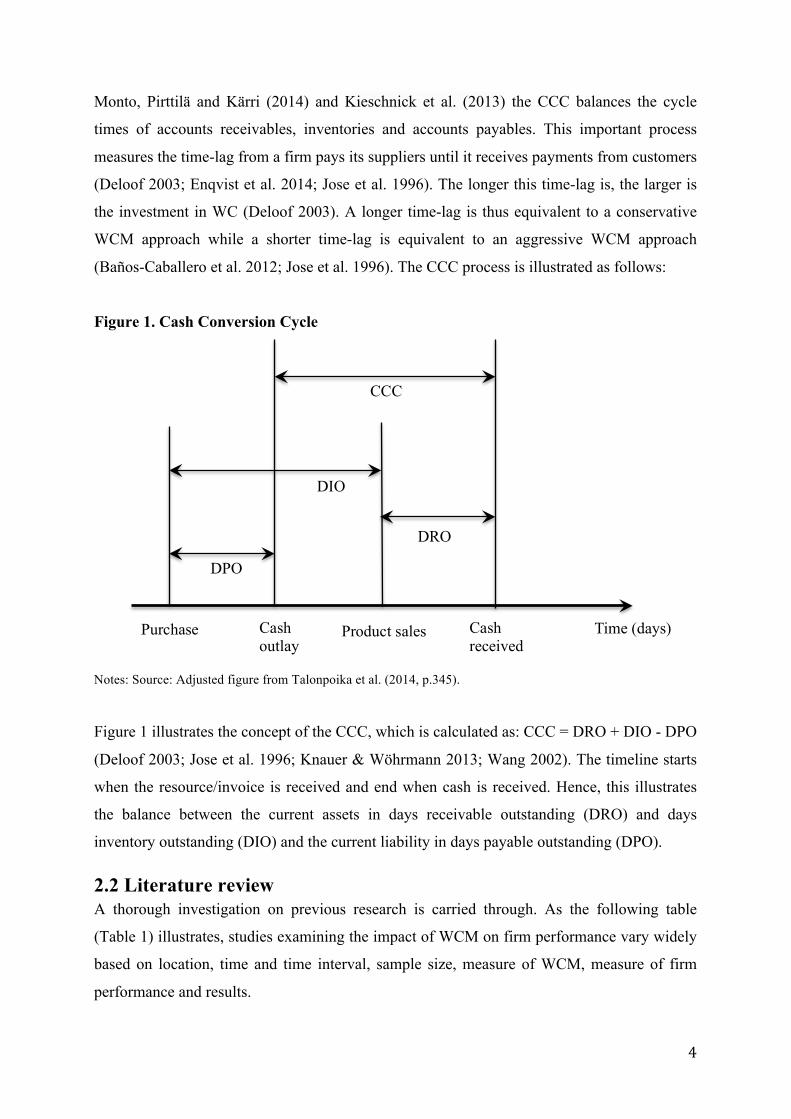
Monto, Pirttilä and Kärri (2014) and Kieschnick et al. (2013) the CCC balances the cycle

times of accounts receivables, inventories and accounts payables. This important process

measures the time-lag from a firm pays its suppliers until it receives payments from customers

(Deloof 2003; Enqvist et al. 2014; Jose et al. 1996). The longer this time-lag is, the larger is

the investment in WC (Deloof 2003). A longer time-lag is thus equivalent to a conservative

WCM approach while a shorter time-lag is equivalent to an aggressive WCM approach

(Baños-Caballero et al. 2012; Jose et al. 1996). The CCC process is illustrated as follows:

Figure 1. Cash Conversion Cycle

Notes: Source: Adjusted figure from Talonpoika et al. (2014, p.345).

Figure 1 illustrates the concept of the CCC, which is calculated as: CCC = DRO + DIO - DPO

(Deloof 2003; Jose et al. 1996; Knauer & Wöhrmann 2013; Wang 2002). The timeline starts

when the resource/invoice is received and end when cash is received. Hence, this illustrates

the balance between the current assets in days receivable outstanding (DRO) and days

inventory outstanding (DIO) and the current liability in days payable outstanding (DPO).

2.2 Literature review A thorough investigation on previous research is carried through. As the following table

(Table 1) illustrates, studies examining the impact of WCM on firm performance vary widely

based on location, time and time interval, sample size, measure of WCM, measure of firm

performance and results.

DPO

DIO

DRO

CCC

Purchase Cash received

Cash outlay

Product sales Time (days)

! 5!

Table 1. Summary literature review Study Country Period Sample size

(observations) Profitability measure

WCM measure

Result WCM on profitability

DRO, DIO, DPO on profitability

Afrifa (2016) UK 2004-2013 65 244 firm-years ROA NWC Concave, but convex when cash flow considers

N/A

Aktas et al. (2015)

US 1982-2011 140 508 firm-years

ROA Excess NWC Concave N/A

Yazdanfar & Öhman (2014)

Sweden 2008-2011 55 188 firm-years ROA CCC CCC!↓ N/A

Enqvist et al. (2014)

Finland 1990-2008 1 136 firm-years ROA GOI

CCC CCC!↓ DRO!→ DIO ↓ DPO ↓

Baños-Caballero et al. (2012)

Spain 2002-2007 5 862 firm-years GOI NOI

CCC Concave N/A

Gill et al. (2010)

US 2005-2007 264 firm-years GOP CCC CCC ↑ DRO ↓ DIO → DPO →

García-Teruel & Martínez-Solano (2007)

Spain 1996-2002 38 464 firm-years ROA CCC CCC!↓ DRO ↓ DIO ↓ DPO →

Lazaridis & Tryfonidis (2006)

Greece 2001-2004 524 firm-years GOP CCC CCC!↓ DRO ↓ DIO → DPO ↑

Deloof (2003) Belgium 1992-1996 5 045 firm-years GOI CCC CCC → DRO ↓ DIO ↓ DPO ↓

Wang (2002) Japan & Taiwan

1985-1996 21 274 firm-years ROE ROA

CCC CCC!↓ N/A

Shin & Soenen (1998)

Global 1975-1994 58 985 firm-years ROA ROS

NTC NTC ↓ N/A

Jose et al. (1996)

US 1974-1993 54 360 firm-years ROA ROE

CCC CCC!↓ N/A

Firm value measure

Result WCM on firm value

DRO, DIO, DPO on firm value

Afrifa (2016) UK 2004-2013 65 244 firm-years Tobin’s Q NWC Concave, but convex when cash flow considers

N/A

Aktas et al. (2015)

US 1982-2011 140 508 firm-years

Excess stock return

Excess NWC Concave N/A

Baños-Caballero et al. (2014)

UK 2001-2007 1 606 firm-years Tobin’s Q NTC Concave N/A

Kieschnick et al. (2013)

US 1990-2006 64 362 firm-years Excess stock return

NWC NWC!↓ N/A

Wang (2002) Japan & Taiwan

1985-1996 21 274 firm-years Tobin’s Q CCC CCC!↓ N/A

Shin & Soenen (1998)

Global 1975-1994 58 985 firm-years Risk-adjusted stock return

NTC NTC!↓ N/A

Table notes: CCC cash conversion cycle, NTC net trade cycle, NWC net working capital, DPO days payable outstanding, DRO days receivable outstanding, DIO days inventory outstanding, ROA return on assets, GOI gross operating income, NOI net operating income, GOP gross operating profit, ROE return on equity, ROS return on sales, ↑, ↓, and →, denotes a significant positive relationship, a significant negative relationship, and no significant relationship based on regression analysis.

! 6!

Table 1 demonstrates that most studies find that a shorter CCC period leads to higher

profitability, although profitability is measured differently in these studies. However, one

study finds that a longer CCC period generates higher profitability (Gill et al. 2010). In

contrast to this, other studies find a concave relationship between the CCC and profitability,

which suggests the existence of an optimal number of days in CCC period. This implies that a

certain level of CCC is positive for higher profitability, while other levels of CCC should

generate a lower profitability (Afrifa 2016; Baños-Caballero et al. 2014). This implies a trade-

off between advantages and disadvantages of CCC periods. Additionally, several of these

studies apply the profitability measures GOP, GOI and ROA. GOP only considers operating

assets and not liabilities. ROA includes financial activities, which could have an impact on the

result when investigating operating activities (Penman 2013).

Five of the studies presented in Table 1 investigate how each of the individual CCC

components affects profitability. Most of these studies find that a shorter DRO and DIO

period is positive for profitability, which is in line with the findings that a lower CCC leads to

higher profitability. The impact of DPO on profitability differs. Two studies find that a lower

DPO is positive for profitability (Deloof 2003; Enqvist et al. 2014). This is contradictory to

the findings that a shorter CCC period leads to a higher profitability because a shorter DPO

period leads to a higher CCC. One study finds that a higher DPO is positive for profitability

(Lazaridis & Tryfonidis 2006).

Studies examining the impact of WCM on market value, measure market value differently.

Shin and Soenen 1998, Kieschnick et al. (2013) and Aktas, Croci and Petmezas (2015) apply

stock return measures, while Wang (2002), Afrifa (2016) and Baños-Caballero et al. (2014)

use Tobin’s Q. These studies also measure WCM differently. NWC, NTC and CCC are the

different measured used. This complicates a comparison between these previous studies.

Some of these studies find support for a negative impact of the WCM measure on market

value, while the rest find support for the existence of an optimal level. These studies only

measure the accumulated CCC period and not the individual CCC components affect market

value.

2.2.1 Arguments for a higher/lower accumulated CCC That a higher CCC hurts profitability is the traditional view (Shin & Soenen 1998).

Mauboussin and Callahan (2014) strengthen this by stating that a lower CCC is associated

with greater operating returns on capital. Mauboussin and Callahan (2014) further claim that

! 7!

this relationship is strongly rooted in academic research. In addition, firms can accomplish a

negative CCC, which means that the firm receives payments from its customers before paying

the suppliers (Mauboussin & Callahan 2014; Farris & Hutchison 2002). This scenario makes

suppliers a source of financing (Mauboussin & Callahan 2014). A lower CCC also reduces

the need to raise external finance, which according to Myers and Majluf (1984) is more

expensive than internal finance. A lower CCC likewise improves the firm’s debt capacity as

less capital needs for financing (Jose et al. 1996).

Baños-Caballero et al. (2012; 2014) and Enqvist et al. (2014) argue that an optimal level of

the CCC could exist, which suggests a balance of costs and benefits of tying up cash in WC.

Hence, the right balance could maximize profitability and firm value. This means that other

levels are not optimal and would generate lower firm performance. This is in line with Filbeck

and Krueger (2005) who claim that a firm’s CCC level consists of a balance between

efficiency and risk. Consequently, it is not risk-free to with a lower CCC. Lower levels of

inventories and receivables might for example lead to lower sales, while higher levels of

payables might lead to lost discounts, which will be elaborated further in Section (2.2.2),

(2.2.3) and (2.2.4).

2.2.2 Arguments for a higher/lower DRO Most studies find that a lower DRO leads to higher profitability. This implies that a lower

collection period of accounts receivables improves profitability, which could be accomplished

by denying credit to customers that need more time to pay for the purchased products

(Sartoris & Hill 1983). However, lower DRO might also impair firm performance. For

example, if a firm decides to shorten credit terms to customers to fulfill a shorter average

collection period it could hurt the sales volume (García-Teruel & Martínez-Solano 2007). If a

firm rather decides to invest more in receivables, the sales could increase (Banos-Caballero et

al. 2012; Yazdanfar & Öhman 2015). Investments in receivables are often associated with

higher sales because they provide customers longer time to pay, which allows the customers

to assess the quality of the products before payment (Long, Malitz & Ravid 1993). Extending

credit terms to customers could also attract new buyers and thus boost sales and reduce

inventories (Yazdanfar & Öhman 2015).

2.2.3 Arguments for a higher/lower DIO Several studies find a significantly negative impact of DIO on profitability. However, an

increase in inventory can actually reduce costs. When a firm holds more inventories it can

! 8!

speculate on price movements (Blinder & Maccini 1991). The firm can thus buy inventories

when prices are low. Buying inventories in large quantities can likewise reduce purchasing

costs (Blinder & Maccini 1991). When sales are fluctuating larger levels of inventories can

help smooth production (Blinder & Maccini 1991; Schiff & Lieber 1974). This lowers the

production costs (Schiff & Lieber 1974). Interruptions in the production processes can

likewise be prevented by increasing inventories (Blinder & Maccini 1991). Contrary to these

arguments, Kim and Chung (1990) argue that lower inventory levels could lead to lower

costs. Inventories are associated with costs for storage, handling, insurance and taxes, hence a

reduction should reduce costs (Kim & Chung 1990). However, the risk of having lower levels

of inventory is that it prevents increased sales (García-Teruel & Martínez-Solano 2007) and

reducing inventories too much could reduce sales due to stock outs (Blinder & Maccini 1991;

Deloof 2003; Jose et al. 1996; Wang 2002).

2.2.4 Arguments for a higher/lower DPO A possible reason why studies find a negative impact of DPO on profitability is that earlier

payments are related to discounts (Deloof 2003; Enqvist et al. 2014; Ng, Smith & Smith

1999; Wilner 2000). Knauer and Wöhrmann (2013) claim that missing discounts as a

consequence of later payments is a reason why studies find negative or insignificant

relationships between DPO and profitability. Enqvist et al. (2014) argue that more profitable

firms often use these discounts rather than use accounts payables as a source of financing.

Additionally, late payments can lead to penalty charges (Gill & Biger 2013). Faster payments

can also strengthen long-term relationships with suppliers (Ng et al. 1999; Wilner 2000).

These arguments imply cost benefits of early payments. However, the study by Lazaridis and

Tryfonidis (2006) find a positive impact of DPO on profitability. A possible reason could be

that accounts payable is an inexpensive and flexible source of financing (Deloof 2003;

Enqvist et al. 2014). It also enables firms to assess the quality of products before payment

(Deloof 2003).

2.3 Performance models Two performance models are presented. The first model illustrates how firm value is created

and the second model how profitability is created. Hypotheses are then formulated based on

the connection between the CCC, the firm performance models and previous research.

2.3.1 Firm value - Discounted Cash Flow (DCF) model To estimate a firm’s market value future activities need to be considered: ”Value today

always equals future cash flow discounted at the opportunity cost of capital” (Brealey, Myers

! 9!

& Allen 2014, p.93). The value of a firm can be calculated by discounting the net of expected

future cash flows generated from investments (Plenborg 2002; Zingales 2000). This is

expressed in the following DCF model where the market value of equity equals the expected

future Free Cash Flow (FCF) attributed to equity holders discounted with the cost of equity.

V!"#$%& =FCF! − Net!cash!flows!to!non!equity!holders

(1+ r!)!!

!!!

Model 1. Discounted Cash Flow, market value of equity. Source: Kieschnick et al. (2013, p.1833).

The market value of equity model is according to Fernandez (2007) one of the most utilized

company valuation models. In Model 1, the FCF simply refers to the amount of cash that is

left from the operational activities after investments in new assets have been deducted

(Penman 2013). This has to be shared among equity and debt holders (Penman 2013). To

obtain the market value of equity the numerator of Model 1 therefore consists of the FCF

minus the Net cash flows to non-equity holders.

When estimating the market value of equity the expected future FCF to equity holders is

simply discounted with the cost of equity capital as shown by Kieschnick et al. (2013). This

cost of equity capital is determined by the operating risk and the financing risk (Penman

2013). Operating risk refers to the risks that operating profits might be hurt. That is the

sensitivity of sales and operating expenses to shocks (Penman 2013). The financing risk is a

function of how highly leveraged the firm is and the difference between the costs of capital

for operations and the cost of capital for debt. The more debt there is and the riskier

operations are in relation to debt, the more risky is the equity (Penman 2013). A firm’s

productive assets are thus evaluated in this valuation model (Jennergren 2008).

Another approach to obtain the FCF is by substituting the change in net operating assets

(NOA) from the operating income (OI): FCF = OI - ∆NOA (Penman 2013). The NOA equal

operating assets (OA) minus operating liabilities (OL): NOA = OA - OL (Penman 2013;

Soliman 2008). Operating assets and liabilities are those assets and liabilities, which are used

in the process of selling to customers. These are the assets that generate OI. OI equals

operating revenue minus operating expense. That is the revenue one obtains when goods or

! 10!

services are sold to customers and the expense, which increases when trading with suppliers

(Penman 2013).

Operating assets and liabilities are contrasted to financing assets and liabilities, which are

used for financing purposes, that is for trading in capital markets (Penman 2013). A firm’s

value is according to Penman (2013) generated by its operations, which is why financial

activities are excluded from the market value model. The distinction between operating assets

and financial assets can be difficult to make. Cash can for example be both an operating and a

financial asset. The operating cash is defined as cash needed as a buffer to pay bills when they

are due. This is a non-interest bearing asset. Other cash give interest and counts as

investments in excess cash, which are referred as financial assets (Penman 2013). This concept to discounting cash flows can also be used by firms in investment decisions

(Brealey et al. 2014). The Net Present Value (NPV) model compares the price of a potential

investment to the expected cash to be generated by the investment during a specific time

interval. The cash that the investment is expected to generate is calculated to a present value

using a discount rate. An investment with a positive NPV is value adding since the value of

the investment exceeds the initial cost (Penman 2013). An investment should only be

accepted if its expected NPV is positive, hence investments with a negative NPV should be

disregarded (Myers & Majluf 1984; Zingales 2000). If the investment is financed by external

or internal funds does not affect the investment decision as a consequence of the assumption

of efficient capital markets (Myers & Majluf 1984).

2.3.2 Firm profitability - DuPont model The DuPont model can be used to illustrate return on net operating assets (RNOA) (Jansen,

Ramnath & Yohn 2011; Penman 2013; Soliman 2008). The concept of this DuPont model is

to set the operating activities in the income statement in relation to the operating components

in the balance sheet (Jansen et al. 2008).

RNOA = ATO!×!PM = !SalesNOA ×OI!(after!tax)

Sales

Model 2. Return on Net Operating Assets. Source: Bauman (2014, p. 193).

Model 2 illustrates how RNOA is obtained by multiplying asset turnover (ATO) with profit

margin (PM). ATO is calculated as sales divided by NOA, and tells how many times the NOA

! 11!

are turned over during a year. PM is calculated as OI after tax divided by Sales (Bauman

2014). Sales is the common variable in the balance sheet ratio and in the income statement

ratio. According to Jansen et al. (2011) income and investments are clearly determined by

sales.

ATO represent the balance sheet in the formula and PM is the contribution from the income

statement, which Soliman (2008) presents as accounting ratios. ATO shows how efficient the

NOA are utilized and is an efficiency measure of different forms of WC (Soliman 2008). In

the area of financial statement analysis, this profitability measure is commonly applied

(Jansen et al. 2011; Soliman 2008). Based on this conceptual model on the relationship

between operational activities on the income statement and the balance sheet we rewrite and

simplify this measure as follows:

RNOA = ATO!×!PM = !SalesNOA ×OI(after!tax)

Sales = Sales!×!OI!(after!tax)NOA!×!Sales = OI!(after!tax)

NOA

Model 3. Return on Net Operating Assets. Source: Adjusted from Bauman (2014, p. 193).

By simplifying the RNOA calculations, the connection between the DuPont model and the

DCF model is clarified and shows RNOA as a function of OI and NOA.

2.4 Hypotheses formulation The CCC, which is a function of accounts receivables, inventories and accounts payables,

affects NOA. NOA impact both the market value of equity and profitability as illustrated in

Section 2.3. Model 1 shows that a change in NOA affects the FCF and consequently the

market value of equity. For example, a decrease in NOA, ceteris paribus, increases the FCF

and hence the market value of equity. This is in line with the argumentation by Talonpoika et

al. (2014), Jose et al. (1996) and Wang (2002) who state that reducing the CCC leads to a

higher net present value of cash flows. This leads to a higher market value (Talonpoika et al.

2014).

On the other hand, based on the argumentation by Penman (2013), the long-term effect on the

FCF by investments in NOA might be the opposite: “For forecasting the long-term, free cash

flow is perverse: investment reduces free cash flow but produces higher future cash flows, so

the lower the free cash flow, the higher are future free cash flows” (p.576). Investments in

WC are however normally viewed as unproductive which is expressed by Afrifa (2016) who

! 12!

argues that this capital could have been invested in other profitable opportunities had it not be

locked up in WC. In line with this, Baños-Caballero et al. (2014) claim that capital tied up in

WC impairs the possibility for firms to make other value-enhancing investments. That

lowering the CCC should improve the market value implies that a lower CCC leads to a

higher market value. A lower CCC also reduces the need for holdings of market securities and

cash, which are viewed as rather unproductive assets (Jose et al. 1996). Furthermore, Wang

(2002) finds that firms with a lower CCC have higher market value than firms with a higher

CCC.

Hypothesis 1a: A lower CCC leads a to higher market value.

A lower level of NOA, which is linked to a lower level of CCC, can also be expected to

generate higher profitability, based on Model 3. This idea are supported by Enqvist et al.

(2014), García-Teruel and Martínez‐Solano (2007), Jose et al. (1996), Kieschnick et al.

(2013), Lazaridis and Tryfonidis (2006), Yazdanfar and Öhman (2014) and Wang (2002) who

find that a lower CCC leads to higher profitability.

Hypothesis 1b: A lower CCC leads to greater profitability.

We have now formulated hypotheses for the accumulated CCC. The following hypotheses are

based on each of the individual CCC components. The first component is DRO. A lower

CCC, that is a lower NOA, can be accomplished by collecting cash from customers quicker.

A lower DRO should thus lead to a higher market value and profitability. This is in line with

the findings by García-Teruel and Martínez‐Solano (2007), Gill et al. (2010) and Deloof

(2003) who find that a shorter DRO period leads to higher profitability.

Hypothesis 2a: A lower DRO leads to a higher market value.

Hypothesis 2b: A lower DRO leads to greater profitability.

A shorter inventory conversion period, ceteris paribus, leads to a lower CCC and less NOA.

This shorter DIO period should lead to a higher market value and profitability in line with

previous discussion. This is consistent with the findings by Enqvist et al. (2014), Deloof

(2013) and García-Teruel and Martínez‐Solano (2007) who find that a lower DIO leads to

higher profitability.

! 13!

Hypothesis 3a: A lower DIO leads to a higher market value.

Hypothesis 3b: A lower DIO leads to greater profitability.

Contrary to the other components of the CCC, a higher DPO leads to a lower CCC. According

to Model 1 and Model 3 a higher DPO should thus lead to a higher market value and

profitability. Findings from previous studies are inconsistent. Lazaridis and Tryfonidis (2006)

however find that a higher DPO leads to higher profitability, which is in line with the

presented performance models.

Hypothesis 4a: A higher DPO leads to a higher market value.

Hypothesis 4b: A higher DPO leads to greater profitability.

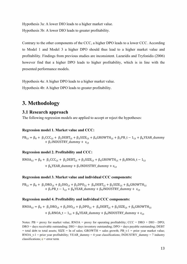
3. Methodology 3.1 Research approach The following regression models are applied to accept or reject the hypotheses:

Regression model 1. Market value and CCC:

PB!,! = β! + !β!CCC!,! + !β!DEBT!,! + β!SIZE!,! + β!GROWTH!,! + β!PB_t − 1!,! + β!YEAR_dummy+ β!INDUSTRY_dummy + !ε!,!

Regression model 2. Profitability and CCC:

RNOA!,! = β! + !β!CCC!,! + !β!DEBT!,! + β!SIZE!,! + β!GROWTH!,! + β!RNOA_t − 1!,!+ β!YEAR_dummy + β!INDUSTRY_dummy + ε!,!

Regression model 3. Market value and individual CCC components:

PB!,! = β! + !β!DRO!,! + β!DIO!,! + β!DPO!,! + !β!DEBT!,! + β!SIZE!,! + β!GROWTH!,!+ β!PB_t − 1!,! + β!YEAR_dummy + β!INDUSTRY_dummy + !ε!,!

Regression model 4. Profitability and individual CCC components:

RNOA!,! = β! + !β!DRO!,! + β!DIO!,! + β!DPO!,! + !β!DEBT!,! + β!SIZE!,! + β!GROWTH!,!+ β!RNOA_t − 1!,! + β!YEAR_dummy + β!INDUSTRY_dummy + ε!,!

Notes: PB = proxy for market value; RNOA = proxy for operating profitability; CCC = DRO + DIO - DPO; DRO = days receivable outstanding; DIO = days inventory outstanding; DPO = days payable outstanding; DEBT = total debt to total assets; SIZE = ln of sales; GROWTH = sales growth; PB_t-1 = prior year market value; RNOA_t-1 = prior year profitability; YEAR_dummy = 4 year classifications; INDUSTRY_dummy = 7 industry classifications; ε = error term

! 14!

The CCC is tested separately and the individual CCC components DRO, DIO and DPO are

included in the same models. Hence, there are two regression models tested for the

performance measure market value and two regression models for profitability. In the

regression models for market value the control variable prior year PB is included, while the

control variable prior year RNOA is included in the regression models for profitability. The

variables included in the regression models are explained in more detail in the following

section.

3.2 Selected variables The balance sheet items in the variables below are calculated as an average of the opening and

closing balance each year, this to make the data compatible with the data in the income

statement which is based on the full year. One exception is the price-to-book ratio which is

calculated using year end data.

3.2.1 WCM efficiency (Independent variables) Applying the CCC enables comparison of WCM efficiency between firms (Mauboussin &

Callahan 2014). The CCC is a common measure of WCM efficiency (see Table 1), and is

calculated as: CCC = DIO + DRO - DPO (Baños-Caballero et al. 2012; Deloof 2003; Jose et

al. 1996). In line with Penman (2013), present paper applies the following calculations of the

individual CCC components:

DRO (Days Receivables Outstanding) = (accounts receivables/(net sales/365)).

DIO (Days Inventory Outstanding) = (inventory/(cost of goods sold/365)).

DPO (Days Payables Outstanding) = (accounts payables/(purchase/365)).

In DPO, purchase is calculated as year-end inventory plus cost of goods sold minus inventory

in the beginning of the year.

The CCC is a comprehensive measure of WCM (Deloof 2003; Enqvist et al. 2014). Jose et al.

(1996) argue that the CCC is dynamic because it includes information from firms’ income

statements as well as balance sheets. In addition, the CCC constitutes of operational activities

(Talonpoika et al. 2014). Considering the three parts of the CCC jointly is important because

they do not only influence profitability and market value, these components also influence

each other (Baños-Caballero et al. 2012; Kieschnick et al. 2013; Kim & Chung 1990; Sartoris

& Hill 1983; Schiff & Lieber 1973).

! 15!

Moreover, Knauer and Wöhrmann (2013) claim that it is important to investigate which

components of the CCC impact firm performance and to what degree, and a study that only

uses the aggregate measure can only speculate. Based on this, the present study examines the

relationship between the individual components of the CCC and firm performance in addition

to the aggregated CCC.

3.2.2 Firm performance - Why two different measures Profitability is the most applied performance measure in the research area investigating the

impact of WCM on firm performance (see Table 1). However, Knauer and Wöhrmann (2013)

stress that profitability as a performance measure is generally problematic because it does not

show the complete picture of firm performance. Knauer and Wöhrmann (2013) therefore

promote using firm value as an alternative measure of firm performance. Profitability is based

on actual accounting data presented in financial statements, while the market value also

consider future predictions (Jennergren 2008; Plenborg 2002; Zingales 2000). Hence, one

problem with profitability as a proxy for firm performance is the time horizon, profitability is

not affected by future potential. A firm can implement a lucrative investment with a positive

NPV that does not improve profitability the first year. The market value is rather affected by

future activities, and thus estimates more accurately the return on this investment.

These performance measures could therefore complement each other. According to Baños-

Caballero et al. (2014) is the empirical evidence regarding the effect of WCM on firm value

scarce, although increased attention has turned to it recently (see Table 1). Present study

therefore includes a measure of market value as a proxy for firm performance as suggested by

Knauer and Wöhrmann (2013), while profitability includes for comparison.

3.2.3 Market valuation (Dependent variable) We use the price-to-book (PB) ratio defined by Penman (2013) as: market value of

equity/book value of equity. This ratio is calculated by using year-end data of: Market

cap/total equity. This measure of market value is similar to the Tobin’s Q ratio used by Afrifa

(2016), Banos-Caballero et al. (2014) and Wang (2002) which is: ((Market value of

equity+book value of debt)/(book value of assets). By removing the book value of debt from

the Tobin’s Q equation present study acquires the PB ratio.

The difference between the market value of equity and the book value of equity is according

to Plenborg (2002) a consequence of investors predictions of potential greater return on equity

! 16!

compared to cost of equity capital. Thus, if investors predict a greater return on equity than

the cost of this capital they are willing to pay a price above the book value of equity (Plenborg

2002). Afrifa (2016) states that Tobin's Q is a market-based measure of financial

performance, which is also true for the PB ratio. The PB ratio is suitable to the market value

of equity model (Model 1), because the numerator in the PB ratio is the market value of

equity. Present study thus expects a higher PB ratio when the market value of equity increases

and vice versa.

3.2.4 Profitability (Dependent variable) Profitability is the second performance measure in the present study. To measure profitability

this study applies RNOA, which measures as follows: OI after tax/NOA = (OI after tax/(OA-

OL)) (Penman 2013). Furthermore, total assets equals operating assets plus financial assets

according to Penman (2013). Financial assets are defined as long- and short-term interest-

bearing assets and calculated as: cash and short-term investments + long-term financial assets.

Operating assets are calculated as: total assets - cash and short-term investments - long-term

financial assets. Moreover, Penman (2013) divides total liabilities and equity into three parts:

operating liabilities, financial obligations and shareholders equity. In line with this, operating

liabilities calculates as: total assets - total debt - total equity. These calculations are similar to

the calculations presented by Soliman (2008).

The most frequently used measure of profitability in this field of study is return on assets

(ROA) (see Table 1). ROA includes both financial and operating activities, which could be a

potential problem when investigating operating activities (Penman 2013). Based on this,

RNOA should be an adequate measure of profitability to study WCM, since this measure

excludes both financial assets and the financial activity in the income statement. RNOA can

thus be considered a measure of operating performance while ROA indicates overall

profitability (Enqvist et al. 2014). Gross operating profit (GOP) is an operating profitability

measure used by other studies (see Table 1). The problem with GOP is that it does not

measure net operating assets and thus GOP does not take operating liabilities into account. In

the denominator of RNOA, on the other hand, both operating assets and liabilities are

considered.

3.2.5 Control variables To control for other variables’ impact on profitability and market value, control variables are

included in the regressions. In line with Enqvist et al. (2014), Deloof (2003), Lazaridis and

! 17!

Tryfonidis (2006), and Shin and Soenen (1998) the debt ratio (DEBT) is applied as a control

variable. As Enqvist et al. (2014), Deloof (2003) and Lazaridis and Tryfonidis (2006) we

calculate DEBT as: total debt/total assets. Deloof (2003) and Enqvist et al. (2014) find that

DEBT affects profitability negatively, which means that a lower grade of debt leads to higher

profitability. According to Koralun-Bereznicka (2014) have firms with a higher debt ratio

often a more aggressive CCC approach.

Additionally, present study includes firm size (SIZE) as a control variable. Enqvist et al.

(2014), Deloof (2003) and García-Teruel and Martínez-Solano (2007) also use this control

variable. Enqvist et al. (2014) and Deloof (2003) measure firm size as the natural logarithm of

sales, while García-Teruel and Martínez-Solano (2007) measure firm size as the logarithm of

assets. We use SIZE measured as the natural logarithm of net sales in thousands SEK. The

difference in asset structure among firms could disrupt the data, and therefore assets are not

used as a measure of firm size. According to Yazdanfar and Öhman (2014) performance can

be affected positively by a firm’s size. Large firms often have a lower CCC and a higher

profitability than small firms (Jose et al. 1996).

Furthermore, present paper controls for potential effects of industry differences. To control

for this, industry dummy variables (INDUSTRY_dummy) are applied. Financial firms such as

banks and insurance companies are excluded, which complies with Deloof (2003), Yazdanfar

and Öhman (2014), Lazaridis and Tryfonidis (2006) and Aktas et al. (2015) because of the

special nature of these firms’ activities. The remaining companies are categorized into seven

industries: construction (D1), manufacturing (D2), natural resources (D3), real estate

management (D4), research & development (D5), retail/wholesale (D6), services (D7). These

industry classifications are constructed based upon the classifications in the databases

Business Retriever and Eikon Datastream. Koralun-Bereznicka (2014) claims that there is a

clear difference among different industries concerning strategies and requirements of WCM.

Wang (2002) finds a clear difference in the CCC among different industries, which

strengthens the importance of controlling for industries.

In line with Deloof (2003), García-Teruel and Martínez-Solano (2007) and Afrifa (2016) sales

growth (GROWTH) is applied as a control variable. GROWTH is measured as: ((this year's

net sales - previous year's net sales)/previous year’s net sales). Deloof (2003) finds a positive

relationship between profitability and sales growth. Afrifa (2016) also finds a highly

! 18!

significant positive relationship between GROWTH and ROA. According to Kieschnick et al.

(2013) an investment in inventory and thus in WC could impact future sales growth because

of the availability of finished products.

In contrast to previous research in the area this study also includes prior year performance

(PB_t-1; RNOA_t-1) as a control variable. Nissim and Penman (2001) show how a large part

of profitability is persistent. A firm’s profitability one year is thus a strong indicator of future

profitability, which is why this is adequate to control for. Additionally, the present paper

controls for year-specific effects by including four year dummies (YEAR_dummy). This is to

control for potential external effects.

! 19!

Table 2. Summary of the applied variables Variable Code Variable type Definition Formula

WCM efficiency

Cash conversion cycle

CCC Independent Time interval of converting purchased material to cash

DRO + DIO - DPO

Days receivables outstanding

DRO Independent Time interval of receiving payments from customer for sold products

Accounts Receivables /(Sales/365)

Days inventory outstanding

DIO Independent Time to turnover the inventory

Inventory/(COGS/365)

Days payable outstanding

DPO Independent Time interval of payment to suppliers for purchased material and products

Accounts Payables /(Purchase/365)

Firm performance

Market value PB Dependent How the market values firms’ equity compared with the booked value of equity

Market value of equity /booked value of equity

Profitability RNOA Dependent Is generated by profit margin and asset turnover, does only consider operating activities

OI (after tax) / (OA-OL)

Other

Debt grade DEBT Control variable To what extent the firm is financed by debt

Total Debt/Total Assets

Firm size

SIZE Control variable

The volume of sales is the measure of firm size

Natural logarithm of sales

Industry (7 categories)

INDUSTRY_dummy

Control variable (Dummy)

Industry classification due to firms characteristics

See definition of industries are divided

Year YEAR_ dummy

Control variable (Dummy)

Year specific effects The data is categorized into each year observed

Sales Growth GROWTH Control variable The annual sales growth (Year 1-Year 0)/Year 0

Market value Prior year

PB_t-1 Control variable Prior year market value of equity to book value of equity

Previous year: Market value of equity /booked value of equity

Profitability Prior year

RNOA_t-1 Control variable Is generated by profit margin and asset turnover, only considers operating activities

Previous year: OI (after tax) / (OA-OL)

Table notes: COGS = Cost of Goods Sold, TA = Total assets, OI= Operating income, OA= Operating assets, OL= Operating liabilities Year 1 = Current year’s sales, Year 0 = previous year’s sales.

3.3 Data We collect data of firms listed on Nasdaq Stockholm OMX (large cap, mid cap and small

cap). The firms’ listed on Nasdaq Stockholm OMX (large cap, mid cap and small cap)

constitute a large share of Swedish listed firms with a total market value of 98 percent of the

market value of all Swedish listed firms (Sveriges Riksbank 2016). 258 non-financial firms

are listed on Nasdaq Stockholm OMX (large cap, mid cap and small cap) according to the

database Retriever Business. These firms are included in the study. The sample extends over

! 20!

four years, from 2012 to 2015. To find patterns, secondary data is collected from databases.

Most of the raw data is collected from the database Retriever Business. From this database we

collect data on net sales, operating income after tax, inventory, accounts receivables, accounts

payables, total assets, total equity and long-term financial assets. The rest of the raw data

required is unavailable or missing for many firms in Retriever Business. The rest of the raw

data is therefore collected from the database Eikon Datastream. From Eikon Datastream data

on cost of goods sold, cash and short-term investments, total debt and market cap is collected

(see Appendix 1).

Out of the 258 non-financial firms listed on Nasdaq Stockholm OMX, 182 have all the raw

data available from 2012 to 2015. Only these firms are included in the study in line with

Deloof (2003), Lazaridis and Tryfonidis (2006) and Wang (2002). This might bias the results

since firms that went bankrupt during the investigation period are not included in the study.

However, the fact that the investigation period only extends over four years lowers this

impact. After this, 728 firm year observations constitute the data set. The data is verified by

checking against annual reports, the data is concluded as reliable. In some cases it is however

obvious that the data is incorrect in which cases the data is adjusted according to the annual

reports. This especially occurs for some items with values of 0. The next step is to calculate

the dependent, independent and control variables using this raw data.

After the variables are calculated, 21 observations contain error values. These observations

have 0 values on cost of goods sold or net sales, which makes the calculation of the CCC

impossible to carry through. These observations are deleted and after this process the data

constitutes 707 firm year observations. Furthermore, all variables except dummy variables are

tested for outliers in SPSS. SPSS defines outliers as data points with values that are lower

than: (Percentile 25 - Interquartile range * 1.5) or higher than: (Percentile 75 + Interquartile

range * 1.5) (Pallant 2013). Pallant (2013) also states that SPSS defines extreme outliers as

observations with values that are lower than: (Percentile 25 - Interquartile range * 3) or higher

than: (Percentile 75 + Interquartile range * 3). As Shin and Soenen (1998) we are worried that

the analysis might be influenced too much by errors if the extreme outlier observations are

unchanged. Another benefit of changing extreme values is that the assumptions made in

multiple regressions are improved. These extreme outliers are winsorized at (Percentile 25 -

Interquartile range * 3) and (Percentile 75 + Interquartile range * 3) which is one way to

handle them (Pallant 2013; Tabachnick & Fidell 2013).

! 21!

Pallant (2013) states that multicollinearity, which means highly correlated independent

variables, impairs regression models. The correlation matrix (Table 4) illustrates that

correlations among the independent variables are weak to moderate. The highest correlations

are between the CCC and its individual components. This is not a problem since these

variables are not included in the same regression models. Moreover, the collinearity

diagnostics in the regression results show that the variance inflation factor (VIF) (see

Appendix 2) takes values well below 10, which would indicate multicollinearity according to

Pallant (2013).

Multiple regressions assume normality, linearity and homoscedasticity of the data (Pallant

2013). These assumptions can be checked using scatterplots (see Appendix 3) (Pallant 2013;

Tabachnick & Fidell 2013). The scatterplots show that the residuals tend to pile up in the

center while deviations from the center are in all directions. This indicates that the normality

assumption is not violated. The scatterplots also show linear tendencies, which indicates that

the assumption of linearity is not violated. The scatterplots also do not show any clear

violation of the homoscedasticity assumption.

! 22!

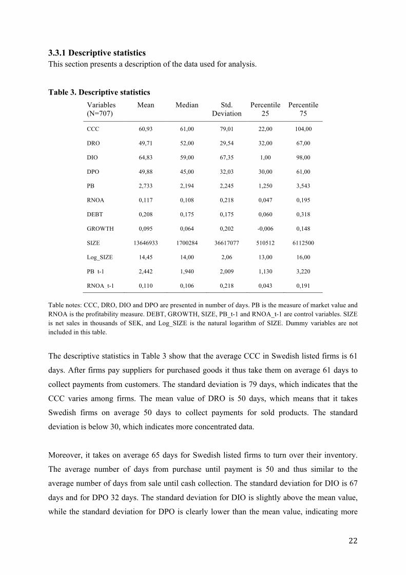
3.3.1 Descriptive statistics This section presents a description of the data used for analysis.

Table 3. Descriptive statistics Variables (N=707)

Mean Median Std. Deviation

Percentile 25

Percentile 75

CCC 60,93 61,00 79,01 22,00 104,00

DRO 49,71 52,00 29,54 32,00 67,00

DIO 64,83 59,00 67,35 1,00 98,00

DPO 49,88 45,00 32,03 30,00 61,00

PB 2,733 2,194 2,245 1,250 3,543

RNOA 0,117 0,108 0,218 0,047 0,195

DEBT 0,208 0,175 0,175 0,060 0,318

GROWTH 0,095 0,064 0,202 -0,006 0,148

SIZE 13646933 1700284 36617077 510512 6112500

Log_SIZE 14,45 14,00 2,06 13,00 16,00

PB_t-1 2,442 1,940 2,009 1,130 3,220

RNOA_t-1 0,110 0,106 0,218 0,043 0,191

Table notes: CCC, DRO, DIO and DPO are presented in number of days. PB is the measure of market value and RNOA is the profitability measure. DEBT, GROWTH, SIZE, PB_t-1 and RNOA_t-1 are control variables. SIZE is net sales in thousands of SEK, and Log_SIZE is the natural logarithm of SIZE. Dummy variables are not included in this table.

The descriptive statistics in Table 3 show that the average CCC in Swedish listed firms is 61

days. After firms pay suppliers for purchased goods it thus take them on average 61 days to

collect payments from customers. The standard deviation is 79 days, which indicates that the

CCC varies among firms. The mean value of DRO is 50 days, which means that it takes

Swedish firms on average 50 days to collect payments for sold products. The standard

deviation is below 30, which indicates more concentrated data.

Moreover, it takes on average 65 days for Swedish listed firms to turn over their inventory.

The average number of days from purchase until payment is 50 and thus similar to the

average number of days from sale until cash collection. The standard deviation for DIO is 67

days and for DPO 32 days. The standard deviation for DIO is slightly above the mean value,

while the standard deviation for DPO is clearly lower than the mean value, indicating more

! 23!

concentrated data on DPO than DIO. The median and mean values are similar for all variables

applied in the regressions, which indicates normal distribution of the data.

The average PB ratio is 2,73. The market value of equity is thus on average 2,73 times the

book value of equity. The mean value of RNOA is 0,12, which means that the OI of firms on

average amount to 12 percent of their NOA. The average net sales are 13646933 TSEK. The

average DEBT is 0,208, which means that firms’ debt is on average 20,8 percent of total

assets, while the rest of the assets are financed by equity and other liabilities. The sales

growth is on average 9,5 percent. The mean value of PB_t-1 is 2,44, which is close to the

mean PB. The mean value of RNOA_t-1 is 0,11, which is close to the average RNOA.

The total number of firm year observations is 707. The dummy variables show how many of

these observations are made of firms classified into each industry. Most observations are

based on service (284) and manufacturing (176) firms. After that, most observations are made

of firms in retail/wholesale (88), research & development (77) and real estate management

(60). The fewest number of observations are made of firms classified as construction (12) and

natural resources (10) firms.

3.4 Analytical tools and approaches SPSS (Statistical package for social sciences) is utilized for analyses. First it is used to create

descriptive statistics and a correlation matrix. Then it is used to run OLS multiple regression

analyses, which are used to accept or reject the hypotheses. The five percent significance level

is applied in order to accept or reject the hypotheses.

4. Result and analysis In this section we present our results and analyze the impact of the CCC and its individual

components on firm performance.

4.1 Correlation matrix This correlation discussion contributes by separately comparing the correlations among the

independent variables and by separately comparing the correlations between the dependent

variables. The following correlation matrix illustrates the correlations among the applied

variables except the dummy variables. The correlation matrix does not show cause and effect,

it only shows the relationship between the different variables (Deloof 2003). Correlation

coefficients are always in the interval -1 to +1. A correlation of -1 is a perfectly negative

! 24!

correlation, which means that the variables move in the opposite directions. A value of +1 is a

perfectly positive correlation and thus the variables move in the same direction. A value of

zero means no correlation.

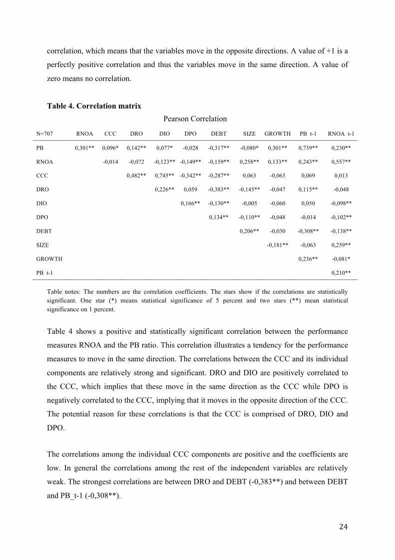
Table 4. Correlation matrix Pearson Correlation

N=707 RNOA CCC DRO DIO DPO DEBT SIZE GROWTH PB_t-1 RNOA_t-1

PB 0,301** 0,096* 0,142** 0,077* -0,028 -0,317** -0,080* 0,301** 0,739** 0,230**

RNOA -0,014 -0,072 -0,123** -0,149** -0,159** 0,258** 0,133** 0,243** 0,557**

CCC 0,482** 0,745** -0,342** -0,287** 0,063 -0,063 0,069 0,013

DRO 0,226** 0,059 -0,383** -0,145** -0,047 0,115** -0,048

DIO 0,166** -0,130** -0,005 -0,060 0,050 -0,098**

DPO 0,134** -0,110** -0,048 -0,014 -0,102**

DEBT 0,206** -0,030 -0,308** -0,138**

SIZE -0,181** -0,063 0,259**

GROWTH 0,236** -0,081*

PB_t-1 0,210**

Table notes: The numbers are the correlation coefficients. The stars show if the correlations are statistically significant. One star (*) means statistical significance of 5 percent and two stars (**) mean statistical significance on 1 percent.

Table 4 shows a positive and statistically significant correlation between the performance

measures RNOA and the PB ratio. This correlation illustrates a tendency for the performance

measures to move in the same direction. The correlations between the CCC and its individual

components are relatively strong and significant. DRO and DIO are positively correlated to

the CCC, which implies that these move in the same direction as the CCC while DPO is

negatively correlated to the CCC, implying that it moves in the opposite direction of the CCC.

The potential reason for these correlations is that the CCC is comprised of DRO, DIO and

DPO.

The correlations among the individual CCC components are positive and the coefficients are

low. In general the correlations among the rest of the independent variables are relatively

weak. The strongest correlations are between DRO and DEBT (-0,383**) and between DEBT

and PB_t-1 (-0,308**).

! 25!

4.2 Regression results

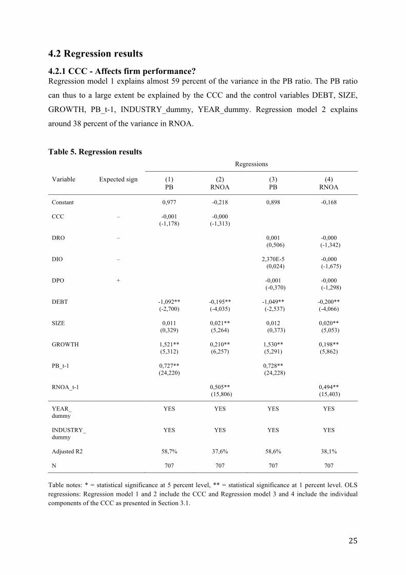
4.2.1 CCC - Affects firm performance? Regression model 1 explains almost 59 percent of the variance in the PB ratio. The PB ratio

can thus to a large extent be explained by the CCC and the control variables DEBT, SIZE,

GROWTH, PB_t-1, INDUSTRY_dummy, YEAR_dummy. Regression model 2 explains

around 38 percent of the variance in RNOA.

Table 5. Regression results Regressions

Variable Expected sign (1) PB

(2) RNOA

(3) PB

(4) RNOA

Constant 0,977 -0,218 0,898 -0,168

CCC – -0,001 (-1,178)

-0,000 (-1,313)

DRO – 0,001 (0,506)

-0,000 (-1,342)

DIO – 2,370E-5 (0,024)

-0,000 (-1,675)

DPO + -0,001 (-0,370)

-0,000 (-1,298)

DEBT -1,092** (-2,700)

-0,195** (-4,035)

-1,049** (-2,537)

-0,200** (-4,066)

SIZE 0,011 (0,329)

0,021** (5,264)

0,012 (0,373)

0,020** (5,053)

GROWTH 1,521** (5,312)

0,210** (6,257)

1,530** (5,291)

0,198** (5,862)

PB_t-1 0,727** (24,220)

0,728** (24,228)

RNOA_t-1 0,505** (15,806)

0,494** (15,403)

YEAR_ dummy

YES YES YES YES

INDUSTRY_dummy

YES YES YES YES

Adjusted R2 58,7% 37,6% 58,6% 38,1%

N 707 707 707 707

Table notes: * = statistical significance at 5 percent level, ** = statistical significance at 1 percent level. OLS regressions: Regression model 1 and 2 include the CCC and Regression model 3 and 4 include the individual components of the CCC as presented in Section 3.1.

! 26!

In the hypotheses formulation in Section 2.4, the present study expects a lower CCC to create

a higher market value and profitability. In line with these predictions, Regression model 1

shows that the CCC has a negative impact on the PB ratio after the effects of the control

variables are controlled for. This impact is however statistically insignificant. Regression

model 2 likewise shows that the CCC has a negative impact on RNOA above and beyond the

impact of the control variables. This impact is also statistically insignificant. The tendency is

thus that a lower CCC leads to higher firm performance but the results are not significant at

the 5 percent level. Based on the insignificance of our findings:

Hypothesis 1a: A lower CCC leads a to higher market value. - Rejected

Hypothesis 1b: A lower CCC leads to greater profitability. - Rejected

A firm’s CCC is higher when its collection period of accounts receivables is longer, when its

inventory conversion period is longer, and when its accounts payable period is shorter. The

traditional view is that higher CCC hurts profitability (Shin & Soenen 1998) and a higher

CCC is equivalent to a larger investment in operating WC (Deloof 2003), thus tying up capital

in WC (Afrifa 2016). Based on the DCF model (Model 1), we derive in the hypotheses

formulation (Section 2.4) that a lower CCC should lead to less NOA, which consequently

should generate a higher FCF and market value. Moreover, a lower CCC should generate

higher profitability based on the DuPont model (Model 3). A possible reason for the

insignificant results is interdependence between NOA and OI. The DCF model (Model 1) and

the DuPont model (Model 3) are both positively influenced by OI. Several arguments are

presented for why a lower CCC might lead to a lower OI and vice versa: lowering inventories

and receivables might reduce sales (Baños-Caballero et al. 2014; Blinder & Maccini 1991;

Deloof 2003; Enqvist et al. 2014; Jose et al. 1996) and increasing payables could lead to lost

discounts (Deloof 2003; Enqvist et al. 2014; Ng et al. 1999; Wilner 2000). Even though a

lower NOA should drive increased market value and profitability, the total effect on firm

performance is therefore unclear.

It is also possible that Swedish listed firms in the same industries have similar WCM

processes, which could explain the insignificant findings. In that case they all have acceptable

CCC levels and the impact on performance could be insignificant. Deloof (2003) also finds an

insignificant impact of the accumulated CCC on profitability. But this insignificant result

differs from other studies, which often find that a lower CCC improves profitability (e.g.

! 27!

García-Teruel & Martínez‐Solano 2007; Jose et al. 1996; Kieschnick et al. 2013; Yazdanfar

& Öhman 2014; Wang 2002). The different profitability measures used could be one reason

to these different results. Present study applies RNOA, which measures operating

profitability, while most of the other studies apply ROA or GOP. The study by Wang (2002)

finds that a lower CCC leads to higher market value. Wang (2002) uses Tobins Q as a

measure of market value that is similar to the PB ratio. The different result on market value

can thus not be explained by the use of a different performance measure. The use of different

performance measures could partly explain the results of the individual CCC components as

well.

Before we proceed with the discussions about the individual components of the CCC, the

regression results of the control variables are presented. DEBT is negatively related to firm

performance in all regressions. Thus, companies with lower debt ratios tend to have a higher

PB ratio and RNOA. The control variable SIZE illustrates that larger companies have

significantly higher RNOA. Larger firms also tend to have a higher PB ratio but this

relationship is insignificant. It is thus not possible to argue that larger firms have higher

market values in relation to their book values. GROWTH is positively related to both

profitability and market value, and statistically significant. Companies with higher sales

growth thus tend to have a higher PB ratio as well as profitability. Unsurprisingly, this is also

true for the relationship between PB_t-1 and PB as it is between RNOA_t-1 and RNOA.

Hence, the performance one year is strongly related to the performance next year.

4.2.2 DRO & DIO – Lower operating assets To further examine the potential impact of WCM on firm performance, the next phase is to

investigate if the individual CCC components have an impact on profitability and market

value. Regression model 3 illustrates that DRO, DIO and DPO together with the control

variables explain almost 59 percent of the variance in the PB ratio. Regression model 4 shows

that DRO, DIO and DPO together with the control variables explain around 38 percent of the

variance in RNOA.

Present study expects that a lower DRO and DIO lead to a higher market value and

profitability. In Regression model 3, where the market value is the dependent variable, the

findings show that the coefficients for DRO and DIO are positive, which is contrary to the

expectations. This positive impact of the DRO and DIO on market value is however highly

! 28!

insignificant. In Regression model 4 with the dependent variable profitability the coefficients

for DRO and DIO are on the other hand negative. This negative impact is also insignificant.

Based on these findings:

Hypothesis 2a: A lower DRO leads to a higher market value. - Rejected

Hypothesis 2b: A lower DRO leads to greater profitability. - Rejected

Hypothesis 3a: A lower DIO leads to a higher market value. - Rejected

Hypothesis 3b: A lower DIO leads to greater profitability. - Rejected

Contrary to these findings, several studies find that a lower DRO and DIO affect profitability

positively (e.g. Deloof 2003; García-Teruel & Martínez-Solano 2007). No studies in the

literature review (Section 2.2) study the impact of DRO or DIO on market value. The results

on the impact of DRO, DIO and DPO on market value in present study can therefore not be

compared to other studies.

The discussion about the CCC illustrates that the CCC may be interconnected with OI.

Likewise, a lower DRO could generate lower OI and a lower DIO could also generate lower

OI. Several arguments are advanced for why a lower DIO could lead to lower OI. Holding

large inventories enable firms to speculate on price movements and buying large quantities

can prevent interruptions in the production process (Blinder & Maccini 1991). Large

inventory levels also enable firms to smooth production when demand is unstable (Blinder &

Maccini 1991; Schiff & Lieber 1974). These are arguments for why lower inventory levels

might lead to higher operating expenses. However, low inventory levels can lead to stockouts

and thus lower sales (Blinder & Maccini 1991; Deloof 2003; Jose et al. 1996; Wang 2002),

which reduces the operating revenue. Further, larger inventory levels generate availability of

complete products, which could lead to future sales growth (Kieschnick et al. 2013).

Additionally, regarding the interdependence between DRO and OI, Banos-Caballero et al.

(2012) argue that firms can increase sales by extending credit days for payments (Banos-

Caballero et al. 2012). This suggests advantages and disadvantages for firms to have longer or

shorter DRO and DIO periods, which indicates an uncertainty of how DRO and DIO affect

firm performance. Hence, this may be one explanation of the insignificant results.

Although the insignificant results, an interesting observation is that the DRO and DIO

coefficients are negative when the dependent variable is profitability and slightly positive

! 29!

when the dependent variable is market value. The NPV model can provide a possible

explanation for this. From the point of view of shareholders, all investments with a positive

NPV increases the market value and the investments should be made. It is possible that

investments that generate a lower profitability than the total profitability of a firm have

positive NPVs. Such investments could affect profitability negatively but market value

positively. That can also be applied to investments in WC. Another possible explanation is

that operating risk may be affected by the management of receivables and inventories, as a

consequence of the risks of lower receivables and inventory levels. The greater amount of

FCF resulting from a reduction in receivables or inventories is thus met by an increased cost

of equity capital, which lowers the market value. A higher risk level does not affect the

profitability and therefore the lower DRO and DIO might separately increase profitability but

not market value.

4.2.3 DPO - Extend trade credit In contrast to account receivables and inventories, a higher DPO is expected to improve firm

performance. Contrary to this expectation Regression model 3 and 4 show a negative but

insignificant impact of DPO on market value and profitability. Based on the insignificance of

our findings:

Hypothesis 4a: A higher DPO leads to a higher market value. - Rejected

Hypothesis 4b: A higher DPO leads to greater profitability. – Rejected

The predictions suggest that a higher DPO should reduce the cumulative CCC, which is in

line with the main concept that higher DPO generates lower aggregate CCC (Knauer &

Wöhrmann 2013). The result shows a tendency for a negative impact of DPO on both market

value and profitability, however these relationships are insignificant in present study. This

negative relationship is similar to the findings by Deloof (2003), Enqvist et al. (2014), and

Lazaridis and Tryfonidis (2006) who find a statistical significant negative impact of DPO on

profitability. This tendency is often explained by the fact that early payments are related to

discounts (Deloof 2003; Enqvist et al. 2014; Ng et al. 1999; Wilner 2000). The reasoning

behind the positive impact of DPO on firm performance, consider not only one-way

agreements but rather that both parts agree of later payments. If the supplier does not accept

later payments for sold products, penalty charges will likely be the consequence, thus

additional interest costs due to the overdue payment (Gill & Biger 2013).

! 30!

Table 6. Outcome of tested hypotheses Hypothesis Independent

variable Dependent

variable Expected outcome

Actual outcome

Significant Accepted/ Rejected

1a CCC PB - - NO Rejected

1b CCC RNOA - - NO Rejected

2a DRO PB - + NO Rejected

2b DRO RNOA - - NO Rejected

3a DIO PB - + NO Rejected

3b DIO RNOA - - NO Rejected

4a DPO PB + - NO Rejected

4b DPO RNOA + - NO Rejected

Table notes: The column with expected outcome illustrates each hypothesis concerning the expected impact of each independent variable on the dependent variable. Actual outcome illustrates the output from the regressions excluding significance level.

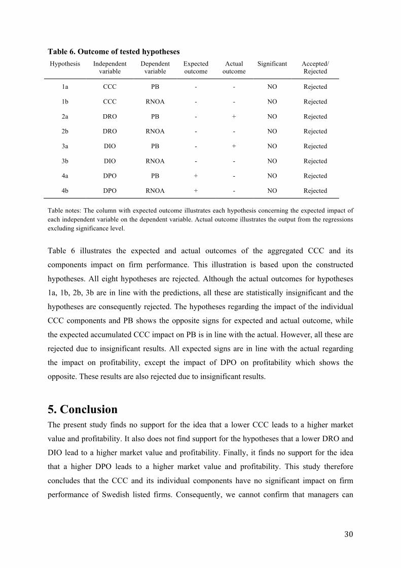
Table 6 illustrates the expected and actual outcomes of the aggregated CCC and its

components impact on firm performance. This illustration is based upon the constructed

hypotheses. All eight hypotheses are rejected. Although the actual outcomes for hypotheses

1a, 1b, 2b, 3b are in line with the predictions, all these are statistically insignificant and the

hypotheses are consequently rejected. The hypotheses regarding the impact of the individual

CCC components and PB shows the opposite signs for expected and actual outcome, while

the expected accumulated CCC impact on PB is in line with the actual. However, all these are

rejected due to insignificant results. All expected signs are in line with the actual regarding

the impact on profitability, except the impact of DPO on profitability which shows the

opposite. These results are also rejected due to insignificant results.

5. Conclusion The present study finds no support for the idea that a lower CCC leads to a higher market

value and profitability. It also does not find support for the hypotheses that a lower DRO and

DIO lead to a higher market value and profitability. Finally, it finds no support for the idea

that a higher DPO leads to a higher market value and profitability. This study therefore

concludes that the CCC and its individual components have no significant impact on firm

performance of Swedish listed firms. Consequently, we cannot confirm that managers can

! 31!

improve firm performance by striving for lower levels of CCC, DIO, DRO or a higher level of

DPO.

A potential reason for the missing impact is that lower levels of CCC, DRO and DIO and

higher levels of DPO might affect OI negatively. The higher market value and profitability

expected from lower levels of NOA could thus be counteracted by a lower OI. The effect on

market value and profitability of having lower levels of NOA is thus uncertain. Another

potential reason for the lack of impact is that Swedish listed firms might have similar

processes for WCM.

6. Future research The present paper has an initial sample of the 258 largest non-financial firms listed in

Sweden. In contrast to most other research in the field of WCM, the present paper is built

upon the DCF model and the DuPont model. Future research could apply these theoretical

models and investigate smaller firms listed in Sweden. A possible reason for the missing

results in this paper is that WCM might be highly standardized in the largest listed firms. It

could therefore be interesting to investigate firms listed on First North, Aktietorget and other

to see if WCM has any impact on their market value and profitability. This potential study

would complement the present study and the study by Yazdanfar and Öhman (2014) in

illustrating the WCM situation in Sweden.

For further investigation it would be interesting with a comparative study between the

Swedish market and one or more markets. This would be interesting since our results are not

in line with the results of studies in other countries.

Most studies about the impact of WCM on firm performance use profitability as a proxy for

firm performance. Our study shows that the impact of WCM on market value might differ

somewhat from that on profitability. It would therefore be of interest for more studies to focus

on the impact of WCM on market value.

7. Acknowledgement We are grateful to our supervisor (Joachim Landström) for the helpful comments, which have

benefited the study.

! 32!

8. References Afrifa, G. A. (2016). Net working capital, cash flow and performance of UK SMEs. Review of Accounting and Finance, 15, 1, pp.21-44.

Aktas, N., Croci, E. & Petmezas, D. (2015). Is working capital management value-enhancing? Evidence from firm performance and investments. Journal of Corporate Finance, 30, pp.98-113.

Baños-Caballero, S., García-Teruel, P. J. & Martínez-Solano, P. (2012). How does working capital management affect the profitability of Spanish SMEs? Small Business Economics, 39, pp.517–529.

Baños-Caballero, S., García-Teruel, P. J., & Martínez-Solano, P. (2014). Working capital management, corporate performance, and financial constraints. Journal of Business Research, 67, 3, pp.332-338.

Bauman, M (2014). Forecasting operating profitability with DuPont analysis: Further evidence. Review of Accounting and Finance, 13, 2, pp.191-205.

Blinder, A. S., & Maccini, L. J. (1991). The resurgence of inventory research: What have

we learned? Journal of Economic Surveys, 5, pp.291–328.

Brealey, R., Myers, S. & Allen, F. (2014). Principles of corporate finance. 11th ed. New York: McGraw-Hill Irwin.

Chiou, J. & Cheng, L. (2006). The determinants of working capital management. Journal of American Academy of Business, 10, pp.149–155.

Deloof, M. (2003). Does Working Capital Management Affect Profitability of Belgian Firms? Journal of Business Finance Accounting, 30, 3-4, pp.573-588.

Enqvist, J., Graham, M. & Nikkinen, J. (2014). The impact of working capital management on firm profitability in different business cycles: Evidence from Finland. Research in International Business and Finance, 32, pp.36-49.

Farris, T. & Hutchison, P. (2002). Cash-to-cash: the new supply chain management metric. International Journal of Physical Distribution & Logistics Management, 32, 4, pp.288-298.

Fernandez, P. (2007). Valuing companies by cash flow discounting: ten methods and nine theories, Managerial Finance, 33, 11, pp.853‐876.

Filbeck, G. & Krueger, T. (2005). An Analysis of Working Capital Management Results Across Industries. American Journal of Business, 20, 2, pp.11-20.

! 33!

García-Teruel, P. J., & Martínez‐Solano, P. (2007). Effects of working capital management on SME profitability. International Journal of Managerial Finance, 3, 2, pp.164-177.

Gill, A., Biger, N. & Mathur, N. (2010). The relationship between working capital management and profitability: evidence from the United States. Business and Economics Journal, 10, 1, pp.1-9.

Gill, A. & Biger, N. (2013). The impact of corporate governance on working capital management efficiency of American manufacturing firms. Managerial Finance, 39, 2, pp.116-132.

Jansen, I., Ramnath, S. & Yohn, T. (2011). A Diagnostic for Earnings Management Using Changes in Asset Turnover and Profit Margin. Contemporary accounting research, 29, 1, pp.221-251.

Jennergren, L. (2008). Continuing value in firm valuation by the discounted cash flow model. European Journal of Operational Research, 185, 3, pp.1548-1563.

Jose, M., Lancaster, C. & Stevens, J.L. (1996). Corporate returns and cash conversion cycles. Journal of Economics and Finance, 20, 1, pp.33-46.

Kieschnick, R., Laplante, M. and Moussawi, R. (2013). Working Capital Management and Shareholders' Wealth. Review of Finance, 17, 5, pp.1827-1852.

Kim, Y. H., & Chung, K. H. (1990). An integrated evaluation of investment in inventory and credit: A cash flow approach. Journal of Business Finance & Accounting, 17, pp.381–390.

Knauer, T. & Wöhrmann, A. (2013). Working capital management and firm profitability. Journal of Management Control, 24, 1, pp.77-78.

Koralun-Bereźnicka, J. (2014). On the relative importance of corporate working capital determinants: findings from the EU countries. Contemporary Economics, 8, 4, pp.415-433.

Lazaridis, I. & Tryfonidis, D. (2006). Relationship between working capital management and profitability of listed companies in the Athens stock exchange. Journal of Financial Management and Analysis, 19, 1, pp.26-35.

Long, M. S., Malitz, I. B., & Ravid, S. A. (1993). Trade credit, quality guarantees, and product marketability. Financial Management, 22, pp.117–127.

Mauboussin, M. J. & Callahan, D. (2014). Capital Allocation: Evidence, Analytical Methods, and Assessment Guidance. Journal of applied corporate finance, 26, 4, pp.48-74.

Myers, S. & Majluf, N. (1984). Corporate financing and investment decisions when firms have information that investors do not have. Journal of Financial Economics, 13, 2, pp.187-221.

! 34!

Nissim, D. & Penman, S. (2001). Ratio Analysis and Equity Valuation: From Research to Practice. Review of Accounting Studies, 6, pp.109-154.

Ng, C., Smith, J. and Smith, R. (1999). Evidence on the Determinants of Credit Terms Used in Interfirm Trade. The Journal of Finance, 54, 3, pp.1109-1129.

Pallant, J (2016). SPSS Survival Manual. 6th ed. Maidenhead: McGraw-Hill Education, 2016.

Penman, S. (2013). Financial statement analysis and security valuation. 5th ed. New York (N.Y.): Mcgraw-Hill.

Plenborg, T. (2002), Firm valuation: comparing the residual income and discounted cash flow approaches. Scandinavian Journal of Management, 18, 3, pp.303‐318.

Sartoris, W. & Hill, N. (1983). A Generalized Cash Flow Approach to Short-Term Financial Decisions. The Journal of Finance, 38, 2, pp.349-360.

Schiff, M. & Lieber, Z. (1974). A model for the integration of credit and inventory management. Journal of Finance, 29, pp.133–140.

Shin, H.H. & Soenen, L. (1998). Efficiency of working capital management and corporate profitability. Financial Practice & Education, 8, 2, pp.39-45.

Soliman, M. (2008). The Use of DuPont Analysis by Market Participants. The Accounting Review, 83, 3, pp.823-853.

Sveriges Riksbank (2016). Den svenska finansmarknaden 2016. Stockholm, August 2016.

http://www.riksbank.se/Documents/Rapporter/Finansmarknaden/2016/rap_finansm_160831_sve.pdf

Tabachnick, B. G. & Fidell, L. S. (2013). Using multivariate statistics (6th edn.). Boston: Pearson Education.

Talonpoika, A. M., Monto, S., Pirttilä, M. & Kärri, T. (2014). Modifying the cash conversion cycle: revealing concealed advance payments. International Journal of Productivity and Performance Management, 63, 3 pp.341-353.

Wang, Y. (2002). Liquidity management, operating performance, and corporate value: evidence from Japan and Taiwan. Journal of Multinational Financial Management, 12, 2, pp.159-169.

Wilner, B. (2000). The Exploitation of Relationships in Financial Distress: The Case of Trade Credit. The Journal of Finance, 55, 1, pp.153-178.

Yazdanfar, D. & Öhman, P. (2014). The impact of cash conversion cycle on firm profitability. International Journal of Managerial Finance, 10, 4, pp.442-452.

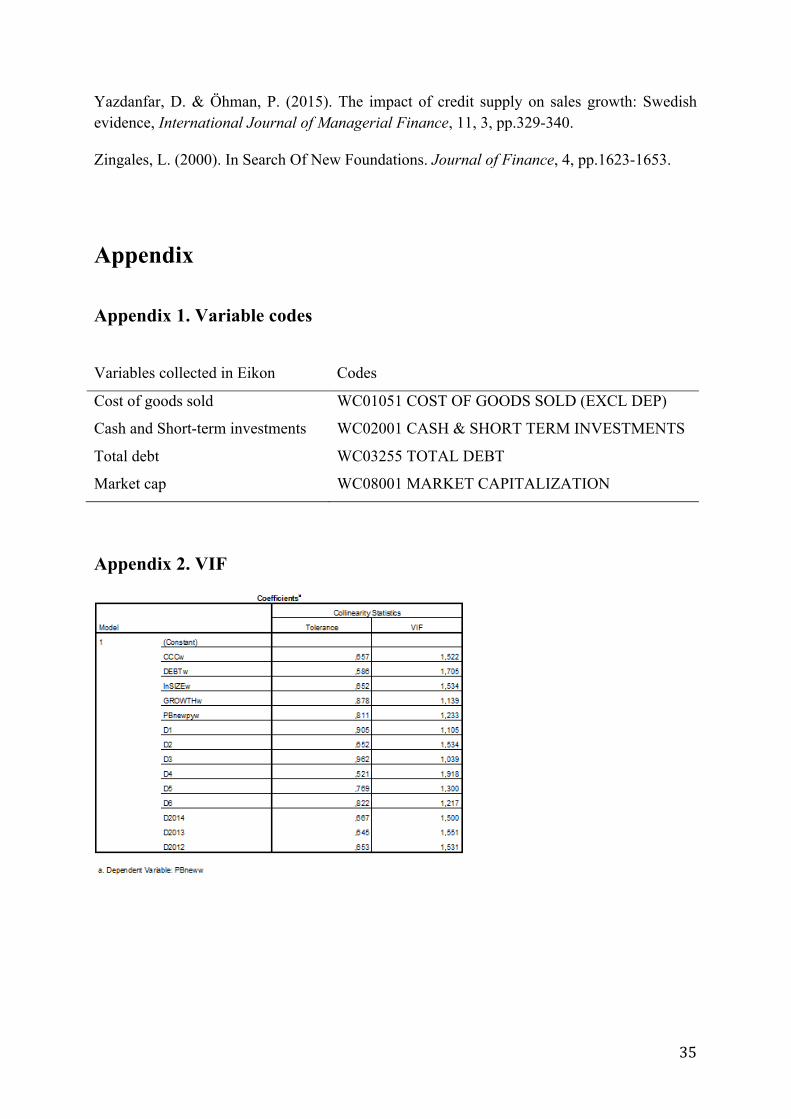
! 35!

Yazdanfar, D. & Öhman, P. (2015). The impact of credit supply on sales growth: Swedish evidence, International Journal of Managerial Finance, 11, 3, pp.329-340.

Zingales, L. (2000). In Search Of New Foundations. Journal of Finance, 4, pp.1623-1653.

Appendix

Appendix 1. Variable codes !!Variables collected in Eikon Codes

Cost of goods sold WC01051 COST OF GOODS SOLD (EXCL DEP)

Cash and Short-term investments WC02001 CASH & SHORT TERM INVESTMENTS

Total debt WC03255 TOTAL DEBT

Market cap WC08001 MARKET CAPITALIZATION

!!

Appendix 2. VIF

! 36!

! 37!

Appendix 3. Scatterplots

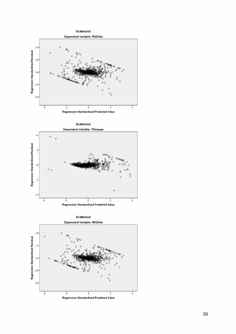
! 38!