Workforce scheduling: A new model incorporating human factors

Journal of Industrial Engineering and Management

JIEM, 2012 – 5(2):259-284 – Online ISSN: 2013-0953 – Print ISSN: 2013-8423

http://dx.doi.org/10.3926/jiem.451

- 259 -

Workforce scheduling: A new model incorporating human factors

Mohammed Othman, Gerard J. Gouw, Nadia Bhuiyan

Concordia University (Canada)

[email protected], [email protected], [email protected]

Received: January 2012 Accepted: September 2012

Abstract:

Purpose: The majority of a company’s improvement comes when the right workers with the

right skills, behaviors and capacities are deployed appropriately throughout a company. This

paper considers a workforce scheduling model including human aspects such as skills, training,

workers’ personalities, workers’ breaks and workers’ fatigue and recovery levels. This model

helps to minimize the hiring, firing, training and overtime costs, minimize the number of fired

workers with high performance, minimize the break time and minimize the average worker’s

fatigue level.

Design/methodology/approach: To achieve this objective, a multi objective mixed integer

programming model is developed to determine the amount of hiring, firing, training and

overtime for each worker type.

Findings: The results indicate that the worker differences should be considered in workforce

scheduling to generate realistic plans with minimum costs. This paper also investigates the

effects of human fatigue and recovery on the performance of the production systems.

Research limitations/implications: In this research, there are some assumptions that might

affect the accuracy of the model such as the assumption of certainty of the demand in each

period, and the linearity function of Fatigue accumulation and recovery curves. These

assumptions can be relaxed in future work.

Originality/value: In this research, a new model for integrating workers’ differences with

workforce scheduling is proposed. To the authors' knowledge, it is the first time to study the

effects of different important human factors such as human personality, skills and fatigue and

recovery in the workforce scheduling process. This research shows that considering both

mailto:[email protected]



www.omniascience.com

www.jiem.org

Journal of Industrial Engineering and Management – http://dx.doi.org/10.3926/jiem.451

- 260 -

technical and human factors together can reduce the costs in manufacturing systems and

ensure the safety of the workers.

Keywords: fatigue; human factors; personality; workforce scheduling

1. Introduction

Effective workforce scheduling is one of the most critical tasks affecting performance of

manufacturing systems. It is important to assign the right job to the right person at the correct

time. Also, it is very important to have a close match between workers’ skills, attitudes and

strength and his/her tasks he/she performs (for simplicity, we will use he/him hereafter). This

needs an effective workforce scheduling system. This system aims to reduce waste in

employing people, lessen uncertainty about current personnel levels and future needs, and

avoid worker and skills shortages or surpluses by hiring the right workers in appropriate

numbers. Traditional workforce scheduling tools are limited and cumbersome. They are

concerned with ‘head count’ rather than ‘head content’, which prevents the resulting schedule

from being flexible enough to follow the growing demand of fast changing business dynamics

(Birch, O’Brien-Pallas, Alksnis, Tomblin Murphy & Thomson, 2003; Castley, 1996; Jensen,

2002). A major problem with existing models is the absence of the most important human

factors inherent in the production system. As one of the main elements in a production

system, human issues cannot be ignored without significantly reducing the benefits of the

production system. Considering human factors in production planning has the potential to

improve both injury risk and production performance (Neumann & Medbo, 2009; Udo &

Ebiefung, 1999). It is important to integrate human factors early in the production planning

phase because early changes to the product and work are less costly and easier to make than

are late changes. Workforce planning is a systematic identification and analysis of what a

company is going to need in terms of the size, type, and quality of workforce to achieve its

strategic objectives. It determines the right number of the right people in the right place at

the right time. In this paper, a new model for workforce scheduling to support production

planning is developed to achieve better production performance while reducing risks to

operator health. The paper is organized as follows: Section 2 presents a literature review of

human factors and their relation to the planning process. Section 3 describes the workforce

scheduling model formulation and the notation used. Next, Section 4 presents the results and

insights generated from the proposed model. Finally, conclusions and suggestions for future

research directions are summarized in Section 5.

2. Literature review

Human Factors (HF), or ergonomics, has been defined as “the theoretical and fundamental

understanding of human behavior and performance in purposeful interacting socio-technical


- 261 -

systems, and the application of that understanding to the design of interactions in the context

of real settings” (Wilson, 2000). During the last decades, ergonomics have been considered

minimally in building production systems. Most business managers have accepted the idea that

ergonomics are working as protectors of workers, rather than creators of systems (Dul &

Neumann, 2009; Perrow, 1983). They generally associate ergonomics with health and safety

issues rather than with the effectiveness of organizations (Jenkins & Rickards, 2001).

Ergonomics is considered too late in the production system development process, making most

managerial decisions hard to change (Helander 1999; Jensen, 2002; Neumann & Medbo,

2009). Perrow (1983) mentioned that the main problem is that human factors specialists have

limited influence and control within the organizational context. Also, they have no control of

strategic resources and a weak network in and outside of the organization. However, it is

shown that ergonomics can contribute to different company strategies and support the

objectives of different business functions in the organization (Dul & Neumann, 2009). On the

other hand, many ergonomics models have been developed without a clear understanding of

how they could be implemented in a specific company (Butler, 2003; Hagg, 2003). Berglund

and Karltun (2007) studied the effects of the human, technology and organizational aspects on

the outcome of the production scheduling processes. Based on their study, schedulers need to

consider uncertainty, their experience, problem solving, workers’ differences, technical system

limitations, the degree of proximity between employees and their informal authority. Jensen

(2002) presents approaches and tools developed in Scandinavian countries. He explained that

the changes in the ergonomics role inside a company require understanding the organizational

prerequisites. He proposed a political agent in order to complement the roles of an expert and

a facilitator. He also suggested developing studies on the management of ergonomics and

organizational development.

There are many reasons for not considering human issues early into production planning.

Helander (1999) discussed seven common reasons for not considering ergonomics early in the

production system development process. Some of the common misconceptions regarding

ergonomics are that many people think that it is for the design of chairs and that it is just

common sense; the research in ergonomics is too abstract to be useful; people are adaptive,

so there is no need for ergonomics; and the technical system should be designed first before

considering ergonomics. Bidanda, Ariyawonggrat, Needy, Norman, and Tharmmaphornphilas

(2005) mentioned that the major reason is that human issues are typically difficult to quantify.

However, none of these are reasons to not consider human factors early in the production

process.

In reality, there is a tremendous variability in individual capabilities. The result is that most

production system designs ignore the effects of the human differences in production system

design. Buzacott (2002) indicates that individual differences can result in substantial loss in

throughput. Worker differences are a fundamental element to consider when assigning workers


- 262 -

to a workstation on the assembly floor. On the other hand, Broberg (2007) has pointed out

that human factors tools to integrate ergonomics into the design process are not known by

engineers. Some tools for handling human factors in planning are creating digital human

models, integrating ergonomics into predetermined motion time systems and integrating

ergonomics into discrete event simulation (DES). However, DES has been considered to be an

appropriate tool that can incorporate human aspects at the earliest planning stage for optimal

performance (Neumann & Medbo, 2009). Some ideas on how to integrate human performance

modeling with DES in assembly lines are suggested (Siebers, 2004; 2006). Due to the

variation in human performance, there is a need for non-deterministic models of worker

performance. Dul and Neumann (2009) provided a conceptual framework to help ergonomists

in research, education and practice to understand how to support the strategic objectives of a

company. This framework helps ergonomics experts to focus on ergonomics from the point of

view of business performance rather than occupational health and safety.

There have been many interesting developments on the technical side of planning and

scheduling processes. Many researchers considered a few human aspects in their quantitative

models. Da Silva, Figueira, Lisboa, and Barman (2006) developed an aggregate production

planning model that includes workers’ training, legal restrictions on workload and workforce

size. Jamalnia and Soukhakian (2009) have developed a fuzzy multi-objective nonlinear

programming model for aggregate production planning problem in a fuzzy environment.

Learning curve effects have been considered in formulating the model. Wirojanagud, Gel,

Fowler, and Cardy (2007) used the general cognitive ability metric to model individual

difference in efficacy of cross-training and worker productivity. Azizi, Zolfaghari and Liang

(2010) considered workers motivation, learning and forgetting factors and workers' skills to

measure employees’ boredom and skill variations during a production horizon. Corominas,

Olivella and Pastor (2010) have taken into account learning curves and workers experience in

modeling a scheduling problem. Also, researchers utilized mathematical models, heuristics and

simulation to study the impact of cross-training on system performance. Stewart, Webster,

Ahmad and Matson (1994) developed four optimization models for different cross-training

scenarios to assist managers in deciding optimum tactical plans for training and assigning a

workforce according to the skills required by a forecasted production schedule. Felan and Fry

(2001) investigated the concept of a multi-level flexibility workforce using simulation. The

results indicate that it is better to have a combination of workers with high flexibility and

workers with no flexibility rather than employing all workers with equal flexibility. Blumberg

and Pringle (1982) developed a model that can link between worker motivation and productive

performance. In their paper, they suggested that expected work performance of individuals is

determined by three factors: Capacity, Opportunity and Willingness. Jaber and Neumann

(2010) developed a mixed-integer linear programming (MILP) model that describes fatigue and

recovery in dual-resource constrained systems. The results obtained from their model suggest

that short rest breaks after each task, short cycle times and faster recovery rates improve the


- 263 -

system’s performance. Fatigue may be defined as a physical and mental weariness existing in

a person and harmfully affecting the ability to perform work. Worker fatigue can greatly impact

system performance in terms of quality (Eklund, 1997). It can significantly affect human

productivity (Oxenburgh, Marlow, & Oxenburgh, 2004). Inordinately long working hours and

poorly planned shift work can result in employee fatigue.

As discussed above, the literature review demonstrated that most of the work on workforce

planning and scheduling assumed that workers are identical. The problem seems to be

systemic and there is an obvious need to integrate ergonomics processes into the organization

early so that underlying principles can be incorporated. Our research will contribute to the

literature by extending existing models of service workforce planning and scheduling beyond

current capabilities. This model will incorporate human issues such as skills, training, worker

personalities, worker recovery and worker fatigue. Four objective functions are considered in

the proposed model. The first one is cost minimization and the second one is top performance

workforce firing minimization, the third one is idle time minimization and the last one is fatigue

rate minimization. In summary, ergonomics must be implemented concurrently with

production planning in order to improve planning process performance. The problem

description, assumptions and formulation are given in the next section.

3. Mathematical modelling of the multiple-objective workforce scheduling problem

In this paper, we analyze the scheduling problem in a job shop environment consisting of

different machines types, which are grouped into several machine levels depending on many

factors such as the complexity and sophistication of the machine, the quantity of the process

plans available and training budget. For example, if we have three machine levels, machine

level one is the less complicated one and machine level three is the most complicated level.

Worker flexibility can be achieved by using overtime and training. Workers are grouped

according to different human skills and personalities and we have made the assumption that

the number of worker skill levels is equal to the number of machine levels. Personality can be

defined as a dynamic and organized set of characteristics possessed by a person that uniquely

influences his or her cognitions, motivations, and behaviors in various situations. We assume

that each worker will have at least one personality level that can be assigned to a certain

machine level depending on his personal traits such as constructive, creative, dynamic,

educated, efficient, etc. They are grouped within the categories of an individual's miscellaneous

attributes and skills. We divided the skill levels and the personality levels into three levels:

level 1 indicates the lowest level, level 2 indicates the middle level, and level 3 indicates the

highest level. In contemporary psychology, the dimensions of personality which are used to

describe human personality are openness, conscientiousness, extraversion, agreeableness, and

neuroticism. Openness includes characteristics such as curiosity, novelty, imagination, insight

and variety. Conscientiousness is a tendency to show self-discipline and being organized, and


- 264 -

achievement-oriented. Extraversion includes characteristics such as sociability, excitability,

assertiveness, and talkativeness. Agreeableness includes characteristics such as morality,

trust, cooperation, kind and sympathy. Finally, Neuroticism is the tendency to experience

emotional instability, anger, anxiety, sadness and depression. In this paper, these traits are

measured based on percentile scores. Level 1 indicates the range from 0 to 33.3th percentile,

level 2 indicates the range from 33.4 to 66.6 percentile, and level 3 indicates the range from

66.7 to 100th percentile. For example, people with high scores on conscientiousness tend to be

responsible, organized and mindful of details, whereas people with low scores on openness

tend to have less curiosity and more traditional interests. However, people with similar

characteristics are grouped into personality levels, which reduce the variability of considering

individual personality profiles. Special questionnaires can be developed and validated for use in

applied research settings to measure the Big Five domains. If, for example, a worker wants to

improve his skills, training can be used. It can also help the person to grow and develop his

personality traits. Layoffs or hiring new workers affect the performance of the present workers

because they need to be trained to the same level as the previous fired workers. Workers have

a certain capacity during work, which is the maximum endurance time, defined as the length of

time that workers can continue to work without becoming fatigued. It is assumed that

endurance time increases as the personality level is increased. When the productive time

increases, the average workload on the worker increases, so that rest breaks have to be given

for the physiological recovery of a worker. Relaxation allowance is used to assist recovery from

fatigue. It is an addition to the basic time intended to provide the worker with the opportunity

to recover from the physiological and psychological effects of carrying out specified work under

specified conditions. The amount of allowance will depend on the nature of the job, personality

attributes and environment. The proposed mathematical programming model is based on the

following assumptions:

All the objective functions and constraints are linear equations.

The demand in each period is deterministic over time.

Fatigue accumulation and recovery curves are linear over time.

The fraction of maximum load capability is applied continuously by the worker when

performing a task for a period equivalent to the task’s duration.

The length of the break between tasks is not long enough to result in full recovery.

The top performers have skill and personal levels greater than or equal to 2.

The length of the shift work of a worker is less than 12 hours including overtime.

The model presented herein is deterministic and in order to satisfy the total demand of each

period, we are interested in determining:

How many workers to assign to each machine level in each period?

How many workers, with which skill levels, to hire or fire in each period?


- 265 -

How many workers to train from lower skill level to higher one in each period?

How many hours a worker with specific skill and personality level can work on overtime

basis?

How long a worker spends on a task in each period?

How long a break time following any task a worker can take?

3.1. Model characteristics

The model developed is a multi-objective integer programming model that allows a number of

different staffing decisions to be made (e.g. hire, train, fire and overtime) in order to minimize

the sum of hiring, firing, training and overtime costs and minimize the top performance

workers fired over all periods, minimize idle (unproductive) time and minimize the physical

load on the workforce.

3.2. Notation and model variables

In presenting the model, the following notations are used:

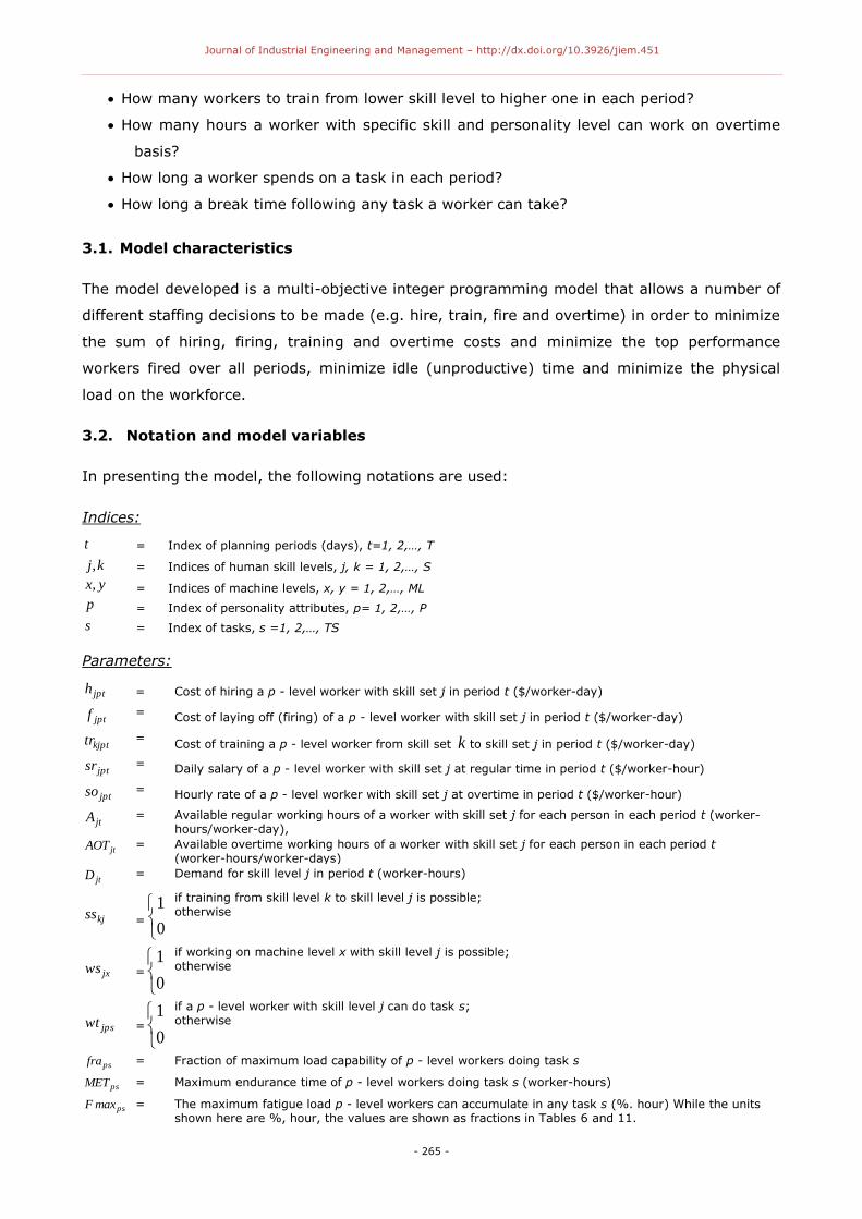
Indices:

t = Index of planning periods (days), t=1, 2,…, T

kj, = Indices of human skill levels, j, k = 1, 2,…, S

yx, = Indices of machine levels, x, y = 1, 2,…, ML

p = Index of personality attributes, p= 1, 2,…, P

s = Index of tasks, s =1, 2,…, TS

Parameters:

jpth = Cost of hiring a p - level worker with skill set j in period t ($/worker-day)

jptf = Cost of laying off (firing) of a p - level worker with skill set j in period t ($/worker-day)

kjpttr

= Cost of training a p - level worker from skill set k to skill set j in period t ($/worker-day)

jptsr = Daily salary of a p - level worker with skill set j at regular time in period t ($/worker-hour)

jptso = Hourly rate of a p - level worker with skill set j at overtime in period t ($/worker-hour)

jtA = Available regular working hours of a worker with skill set j for each person in each period t (worker-hours/worker-day),

jtAOT = Available overtime working hours of a worker with skill set j for each person in each period t

(worker-hours/worker-days)

jtD = Demand for skill level j in period t (worker-hours)

kjss =

0

1

if training from skill level k to skill level j is possible; otherwise

jxws =

0

1

if working on machine level x with skill level j is possible; otherwise

jpswt =

0

1

if a p - level worker with skill level j can do task s;

otherwise

psfra = Fraction of maximum load capability of p - level workers doing task s

psMET = Maximum endurance time of p - level workers doing task s (worker-hours)

psmaxF = The maximum fatigue load p - level workers can accumulate in any task s (%. hour) While the units shown here are %, hour, the values are shown as fractions in Tables 6 and 11.


- 266 -

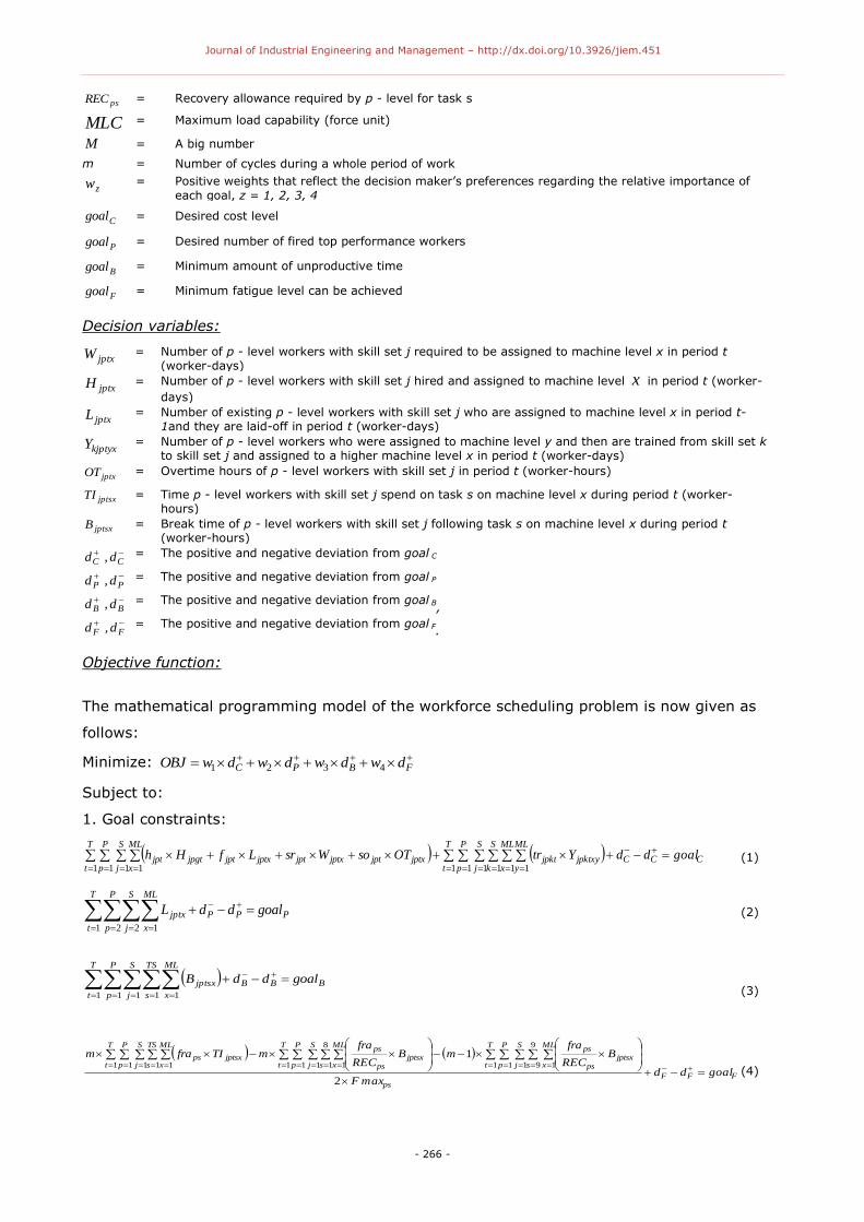
psREC = Recovery allowance required by p - level for task s

MLC

= Maximum load capability (force unit)

M = A big number

m = Number of cycles during a whole period of work

zw = Positive weights that reflect the decision maker’s preferences regarding the relative importance of

each goal, z = 1, 2, 3, 4

Cgoal = Desired cost level

Pgoal = Desired number of fired top performance workers

Bgoal = Minimum amount of unproductive time

Fgoal = Minimum fatigue level can be achieved

Decision variables:

jptxW = Number of p - level workers with skill set j required to be assigned to machine level x in period t (worker-days)

jptxH = Number of p - level workers with skill set j hired and assigned to machine level x in period t (worker-

days)

jptxL = Number of existing p - level workers with skill set j who are assigned to machine level x in period t-1and they are laid-off in period t (worker-days)

kjptyxY

= Number of p - level workers who were assigned to machine level y and then are trained from skill set k to skill set j and assigned to a higher machine level x in period t (worker-days)

jptxOT = Overtime hours of p - level workers with skill set j in period t (worker-hours)

jptsxTI = Time p - level workers with skill set j spend on task s on machine level x during period t (worker-hours)

jptsxB = Break time of p - level workers with skill set j following task s on machine level x during period t

(worker-hours) CC d,d

= The positive and negative deviation from goal C

PP d,d

= The positive and negative deviation from goal P

BB d,d

= The positive and negative deviation from goal B

,

FF d,d

= The positive and negative deviation from goal F

.

Objective function:

The mathematical programming model of the workforce scheduling problem is now given as

follows:

Minimize: FBPC dwdwdwdwOBJ 4321

Subject to:

1. Goal constraints:

T

t

P

p

S

j

S

k

ML

xC

ML

yCCjpktxyjpkt

T

t

P

p

S

j

ML

xjptxjptjptxjptjptxjptjpgtjpt goalddYtrOTsoWsrLfHh

1 1 1 1 1 11 1 1 1

(1)

PPP

T

t

P

p

S

j

ML

x

jptx goalddL

1 2 2 1

(2)

BBB

T

t

P

p

S

j

TS

s

ML

x

jptsx goalddB

1 1 1 1 1

(3)

FFFps

T

t

P

p

S

j s

ML

xjptsx

ps

psT

t

P

p

S

j s

ML

xjptsx

ps

psT

t

P

p

S

j

TS

s

ML

xjptsxps

goalddmaxF

BREC

framB

REC

framTIfram

2

11 1 1

9

9 11 1 1

8

1 11 1 1 1 1

(4)


- 267 -

2. Other constraints:

jt

P

p

P

p

ML

xjptx

TS

sjptsx

ML

xjptxjt DOTBNWA

1 1 111

t,j

(5)

jptx

TS

sjtxjptjptsxjptsx WABNBTIN

19

x,t,p,j (6)

psxjptp

p

s

jptsxps

psTS

s

jptsxps FBREC

framB

REC

framTIfram max1 9

9

98

11

x,t,p,j (7)

j

jjk

k

kjk

y

yxy

jkptxy

x

xxy

kjptyxjptxjptxxjptjptx YYLHWW

21

21

21

21

1 x,t,p,j (8)

jptxjtjptx WAOTOT

x,t,p,j (9)

xtjp

S

jkk

ML

y

jptxjkptxy WLY ,1,

1 1

x,t,p,j (10)

jpxjptx wsML x,t,p,j (11)

jpxjptx wsMH x,t,p,j (12)

kpykjptyx wsMY y,x,t,p,k,j (13)

jpxkjptyx wsMY y,x,t,p,k,j (14)

kjkjptyx ssMY y,x,t,p,k,j (15)

jptx

S

kkjptyx ZMY

1 y,x,t,p,j

(16)

jptxjptx ZML 1

x,t,p,j (17)

jptxjptx UMH

x,t,p,j (18)

jptxjptx UML 1

x,t,p,j (19)

jptxpsjptsx WMETmTI

x,s,t,p,j (20)

jpsjptsx WTMTI

x,s,t,p,j (21)

jptsxpsjptsx TIRECB

x,s,t,p,j (22)

psfra

ps eMET

s,p

(23)

pspspmax METfraMLCF

s,p

(24)

0,,,,,,,,,,,,,,, ffttppccjptsxjptsxjptxkjptyxjptxjptxjptx ddddddddBTIOTYLHW

y,x,t,p,k,j

(25)

1,0, jptxjptx UZ

x,t,p,j (26)


- 268 -

The objective function aims to minimize: all costs incurred including worker hiring and firing,

training costs and overtime costs; the top performer layoffs; idle (unproductive) time; and the

weighted average fatigue rate. The purpose of optimization is to minimize the deviations from

specific goals based on the importance of each one. Constraints (1), (2), (3) and (4) represent

the cost goal, top performance goal, unproductive time goal and fatigue level goal constraints,

respectively. Constraint (5) shows that the total regular time a worker spends on a task plus

the total overtime hours are equal to the number of hours required for each skill in each

period. Constraint (6) shows that the total regular time a worker spends on a task plus the

total breaks and interruptions during should not be greater than the available labour capacity.

Constraint (7) ensures that the fatigue rate at the end of a period has to be less than the

maximum fatigue load a worker can accumulate in any task. Constraint (8) ensures that the

workforce in any period should equal the workforce in the previous period plus the new hires

and is trained to the upper level minus the layoffs. Constraint (9) ensures the overtime

workforce available should be less than the maximum overtime workforce available in each

period. Constraint (10) ensures that the total number of workers who are assigned to machine

level x in period t-1 and now fired or trained for upper skill levels should not be greater than

the number of workers required in the previous period. Constraint (11) ensures that workers

can be fired if and only if the assignment is possible. Constraint (12) denotes that workers can

be hired if and only if the assignment is possible. Constraint (13) ensures that training for

better skills is possible if and only if the previous assignment is possible. Constraint (14)

ensures that training for better skills is possible if and only if the latter assignment is possible.

Constraint (15) ensures that training for better skills is possible if and only if training to that

skill is possible. Constraints (16) and (17) guarantee the workers who are trained for skill level

j should not be fired in the same period. Constraints (18) and (19) ensure that either hiring or

firing workers occurs but not both. Constraint (20) ensures that the processing time for any

task cannot exceed the maximum endurance time for any individual performing that task.

Constraint (21) states that the worker can perform any task if and only if the worker

assignment to that task is possible. Constraint (22) ensures that the break time following any

task is to be less than or equal to the recommended recovery duration for that task. Constraint

(23) calculates the value of maximum endurance time based on the fraction of the maximum

load capability applied when performing certain task. Constraint (24) calculates the total limit

for maximum fatigue index. Finally, constraints (25) and (26) are the non-negativity

constraints.

Goal programming can be used to solve the multi-objective functions. It provides a way of

striving towards conflicting objectives simultaneously. The basic approach of goal programming

is to establish a specific target for each of the objectives, formulate an objective function for

each objective, and then seek a solution that minimizes the (weighted) sum of deviations of

these objective functions from their targets. There are two methods for solving goal programs:

the non-preemptive method (weights method) and the preemptive method. The weights


- 269 -

methods form a single objective function consisting of the weighted sum of the goals, where all

goals are roughly comparable of importance. On the other hand, the preemptive method

organizes the goals one at a time starting with the highest priority goal and terminating with

the lowest one without degrading the quality of a higher-priority goal (Hillier & Lieberman,

2010). In this paper, the non-preemptive method is used to solve the problem. The decision

maker must determine penalty weights that reflect his preferences regarding the relative

importance of each goal. For example, penalty weights equal to 1 signify that all goals carry

equal weights. The determination of the specific values of these weights is subjective. Different

methods have been developed to estimate the weight values (Tamiz, Jones, & Romero, 1998;

Cohon, 1978). The solution procedure considers one goal at a time, starting with the costs

minimization goal, and terminating with the fatigue minimization goal. The process is carried

out such that the solution obtained from a first goal never degrades the other goals solutions.

However, weighted goal programming considers all goals simultaneously within a composite

objective function comprising the sum of all deviational variables of the goals from their

targets. One of the drawbacks of this method is the use of different units of deviational

variables in an objective function where the sums of unwanted deviational variables are

minimized. This different measurement unit may damage the relative importance of the

objective to the decision maker or cause an unintentional bias towards the objectives with a

larger magnitude (Tamiz et al., 1998). This problem can be solved by the use of a

normalization procedure or simply using same unit for all deviational variables in the objective

function. Different normalization techniques are suggested (De Kluyver, 1979; Jones, 1995;

Masud & Hwang, 1981; Wildhelm, 1981). In this research, the following steps are used to

handle multi-objective functions:

Define LP1 as the first Linear programming model with objective function: minimize

goal c ; LP2 is the second linear programming model with objective function: minimize

goal P ; LP3 is the third linear programming model with objective function: minimize

goal B ; LP4 is the fourth linear programming model with objective function: minimize

goal F .

Identify the goal values of each model in step 1, and add these values to the right hand

side of each constraint (1), (2), (3) and (4), respectively, to ensure the goals are

satisfied.

Add penalty weights to reflect the decision maker's preferences regarding the relative

importance of each goal; for example: in order to minimize total costs (goal C), its

penalty weight should be multiplied by the amount over the costs target determined in

step 2. Also, in order to minimize total number of top performers fired (goal P), its


- 270 -

penalty costs should be multiplied by the amount under the desired number that can be

achieved, and so on.

Solve the combined objective function that minimizes the deviational variables which

represents all goals.

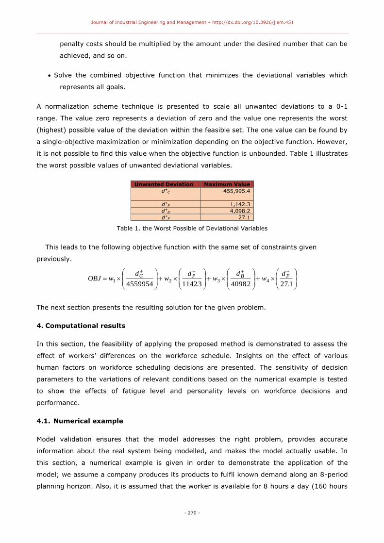
A normalization scheme technique is presented to scale all unwanted deviations to a 0-1

range. The value zero represents a deviation of zero and the value one represents the worst

(highest) possible value of the deviation within the feasible set. The one value can be found by

a single-objective maximization or minimization depending on the objective function. However,

it is not possible to find this value when the objective function is unbounded. Table 1 illustrates

the worst possible values of unwanted deviational variables.

Unwanted Deviation Maximum Value

d+C 455,995.4

d+P 1,142.3

d+B 4,098.2

d+F 27.1

Table 1. the Worst Possible of Deviational Variables

This leads to the following objective function with the same set of constraints given

previously.

127240983114244559954321

.

dw

.

dw

.

dw

.

dwOBJ FBPC

The next section presents the resulting solution for the given problem.

4. Computational results

In this section, the feasibility of applying the proposed method is demonstrated to assess the

effect of workers’ differences on the workforce schedule. Insights on the effect of various

human factors on workforce scheduling decisions are presented. The sensitivity of decision

parameters to the variations of relevant conditions based on the numerical example is tested

to show the effects of fatigue level and personality levels on workforce decisions and

performance.

4.1. Numerical example

Model validation ensures that the model addresses the right problem, provides accurate

information about the real system being modelled, and makes the model actually usable. In

this section, a numerical example is given in order to demonstrate the application of the

model; we assume a company produces its products to fulfil known demand along an 8-period

planning horizon. Also, it is assumed that the worker is available for 8 hours a day (160 hours


- 271 -

per month) at regular time and for 2 hours a day (80 hours per month) at overtime. However,

it is assumed that a worker is not productive during daily breaks and interruptions. Also, the

maximum fatigue load a worker can accumulate in any task depends on the personality level.

Many jobs require human effort, and some recovery allowance must be made from fatigue for

relaxation. We assume that a worker with a high personality level and in top physical condition

requires a smaller allowance to recover from fatigue than a low personality level worker.

However, other factors such as the factors related to the nature of the work itself and the

environment might affect the amount of relaxation allowances needed. Moreover, input data is

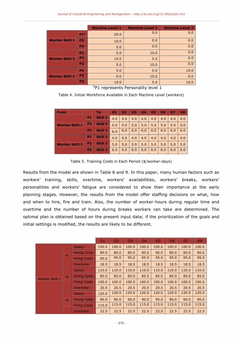
shown in Tables 2 to 7. The known demand of worker skills in worker-hours in each period is

summarized in Table 2. Table 3 shows workers’ availabilities. Table 4 shows the available

workforce at period zero. Next, Table 5 shows the cost of training from skill level to another

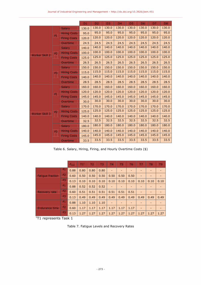
skill level in each period. Workers daily salary, hiring costs, lay-off costs, overtime costs and

workers’ capacities are shown in Table 6. Finally, Table 7 shows the values of the maximum

endurance time, fatigue fractions and the recovery rates for different workers. These values

are estimated based on the formulas, which are adapted from Jaber and Neumann (2010).

Using the input data presented, the model consists of 7,364 variables and 12,929 constraints

and the optimal solution for the problem can be easily obtained using LINGO 13.0 software in

less than a minute of program running.

D1a D2 D3 D4 D5 D6 D7 D8

Worker Skill 1 320.0 160.0 320.0 320.0 320.0 320.0 320.0 320.0

Worker Skill 2 400.0 320.0 320.0 320.0 400.0 160.0 320.0 480.0

Worker Skill 3 400.0 480.0 480.0 480.0 320.0 160.0 320.0 320.0

aD1 represents Day 1

Table 2. Demand of Worker Skills in Each Week (worker-hours)

D1 D2 D3 D4 D5 D6 D7 D8

Worker Skill 1 Availability (regular time) 8.0 8.0 8.0 8.0 8.0 8.0 8.0 8.0

Availability (overtime) 2.0 2.0 2.0 2.0 2.0 2.0 2.0 2.0





Table 3. Workers’ Availabilities (worker-hours)


- 272 -

Machine Level 1 Machine Level 2 Machine Level 3

Worker Skill 1

P1b 20.0 0.0 0.0

P2

10.0 0.0 0.0

P3

5.0 0.0 0.0

Worker Skill 2

P1 5.0 10.0 0.0

P2

10.0 5.0 0.0

P3

5.0 10.0 0.0

Worker Skill 3

P1 5.0 0.0 10.0

P2

0.0 10.0 0.0

P3

10.0 5.0 10.0 bP1 represents Personality level 1

Table 4. Initial Workforce Available in Each Machine Level (workers)

From To D1 D2 D3 D4 D5 D6 D7 D8

Worker Skill 1

P1 Skill 2 4.0 4.0 4.0 4.0 4.0 4.0 4.0 4.0

P2 Skill 2 5.0 5.0 5.0 5.0 5.0 5.0 5.0 5.0

P3 Skill 2 6.0 6.0 6.0 6.0 6.0 6.0 6.0 6.0

Worker Skill 2

P1 Skill 3 4.0 4.0 4.0 4.0 4.0 4.0 4.0 4.0

P2 Skill 3 5.0 5.0 5.0 5.0 5.0 5.0 5.0 5.0

P3 Skill 3 6.0 6.0 6.0 6.0 6.0 6.0 6.0 6.0

Table 5. Training Costs in Each Period ($/worker-days)

Results from the model are shown in Table 8 and 9. In this paper, many human factors such as

workers’ training, skills, overtime, workers’ availabilities, workers’ breaks, workers’

personalities and workers’ fatigue are considered to show their importance at the early

planning stages. However, the results from the model offer staffing decisions on what, how

and when to hire, fire and train. Also, the number of worker-hours during regular time and

overtime and the number of hours during breaks workers can take are determined. The

optimal plan is obtained based on the present input data; if the prioritization of the goals and

initial settings is modified, the results are likely to be different.

D1 D2 D3 D4 D5 D6 D7 D8

Worker Skill 1

P1

Salary 100.0 100.0 100.0 100.0 100.0 100.0 100.0 100.0

Hiring Costs 80.0 80.0 80.0 80.0 80.0 80.0 80.0 80.0

Firing Costs 95.0 95.0 95.0 95.0 95.0 95.0 95.0 95.0

Overtime 18.5 18.5 18.5 18.5 18.5 18.5 18.5 18.5

P2

Salary 110.0 110.0 110.0 110.0 110.0 110.0 110.0 110.0

Hiring Costs 85.0 85.0 85.0 85.0 85.0 85.0 85.0 85.0

Firing Costs 100.0 100.0 100.0 100.0 100.0 100.0 100.0 100.0

Overtime 20.5 20.5 20.5 20.5 20.5 20.5 20.5 20.5

P3

Salary 120.0 120.0 120.0 120.0 120.0 120.0 120.0 120.0

Hiring Costs 90.0 90.0 90.0 90.0 90.0 90.0 90.0 90.0

Firing Costs 115.0 115.0 115.0 115.0 115.0 115.0 115.0 115.0

Overtime 22.5 22.5 22.5 22.5 22.5 22.5 22.5 22.5


- 273 -

D1 D2 D3 D4 D5 D6 D7 D8

Worker Skill 2

P1

Salary 130.0 130.0 130.0 130.0 130.0 130.0 130.0 130.0

Hiring Costs 95.0 95.0 95.0 95.0 95.0 95.0 95.0 95.0

Firing Costs 120.0 120.0 120.0 120.0 120.0 120.0 120.0 120.0

Overtime 24.5 24.5 24.5 24.5 24.5 24.5 24.5 24.5

P2

Salary 140.0 140.0 140.0 140.0 140.0 140.0 140.0 140.0

Hiring Costs 100.0 100.0 100.0 100.0 100.0 100.0 100.0 100.0

Firing Costs 125.0 125.0 125.0 125.0 125.0 125.0 125.0 125.0

Overtime 26.5 26.5 26.5 26.5 26.5 26.5 26.5 26.5

P3

Salary 150.0 150.0 150.0 150.0 150.0 150.0 150.0 150.0

Hiring Costs 115.0 115.0 115.0 115.0 115.0 115.0 115.0 115.0

Firing Costs 140.0 140.0 140.0 140.0 140.0 140.0 140.0 140.0

Overtime 28.5 28.5 28.5 28.5 28.5 28.5 28.5 28.5

Worker Skill 3

P1

Salary 160.0 160.0 160.0 160.0 160.0 160.0 160.0 160.0

Hiring Costs 120.0 120.0 120.0 120.0 120.0 120.0 120.0 120.0

Firing Costs 145.0 145.0 145.0 145.0 145.0 145.0 145.0 145.0

Overtime 30.0 30.0 30.0 30.0 30.0 30.0 30.0 30.0

P2

Salary 170.0 170.0 170.0 170.0 170.0 170.0 170.0 170.0

Hiring Costs 125.0 125.0 125.0 125.0 125.0 125.0 125.0 125.0

Firing Costs 140.0 140.0 140.0 140.0 140.0 140.0 140.0 140.0

Overtime 32.5 32.5 32.5 32.5 32.5 32.5 32.5 32.5

P3

Salary 180.0 180.0 180.0 180.0 180.0 180.0 180.0 180.0

Hiring Costs 140.0 140.0 140.0 140.0 140.0 140.0 140.0 140.0

Firing Costs 145.0 145.0 145.0 145.0 145.0 145.0 145.0 145.0

Overtime 33.5 33.5 33.5 33.5 33.5 33.5 33.5 33.5

Table 6. Salary, Hiring, Firing, and Hourly Overtime Costs ($)

Fmax T1c T2 T3 T4 T5 T6 T7 T8 T9

Fatigue fraction

P1 0.88 0.80 0.80 0.80 - - - - - -

P2 0.60 0.50 0.50 0.50 0.50 0.50 0.50 - - -

P3 0.13 0.10 0.10 0.10 0.10 0.10 0.10 0.10 0.10 0.10

Recovery rate

P1 0.88 0.52 0.52 0.52 - - - - - -

P2 0.60 0.51 0.51 0.51 0.51 0.51 0.51 - - -

P3 0.13 0.49 0.49 0.49 0.49 0.49 0.49 0.49 0.49 0.49

Endurance time

P1 0.88 1.10 1.10 1.10 - - - - - -

P2 0.60 1.17 1.17 1.17 1.17 1.17 1.17 - - -

P3 0.13 1.27 1.27 1.27 1.27 1.27 1.27 1.27 1.27 1.27

cT1 represents Task 1

Table 7. Fatigue Levels and Recovery Rates


- 274 -

D1 D2 D3 D4 D5 D6 D7 D8

Demand (workers) 40.0 20.0 40.0 40.0 40.0 40.0 40.0 40.0

Worker Skill 1

P1

Workers used on level 1 29.1 22.1 44.2 44.2 44.2 44.2 44.2 44.2

Workers hired on level 1 23.9 0.0 22.1 0.0 11.1 0.0 27.7 22.1

Workers fired from level 1 0.0 7.0 0.0 0.0 0.0 0.0 0.0 0.0

Workers trained to Level 2 14.8 0.0 0.0 0.0 11.1 0.0 27.7 22.1

P2





P3





Demand (workers) 50.0 40.0 40.0 40.0 50.0 20.0 40.0 60.0

Worker Skill 2

P1



Workers hired on level 1&2 0.0 0.0 0.0 0.0 0.0 0.0 0.0 0.0

Workers fired from level 1&2 0.0 0.0 0.0 0.0 0.0 0.0 25.0 0.0


P2






P3






Demand (workers) 50.0 60.0 60.0 60.0 40.0 20.0 40.0 40.0

Worker Skill 3

P1



Workers used on level 3 14.8

25.9 25.9 25.9 8.8 0.0 0.0 0.0

Workers hired on level 1,2&3 0.0 0.0 0.0 0.0 0.0 0.0 0.0 0.0

Workers fired from level 1&2&3 0.0 0.0 0.0 0.0 17.1 13.8 0.0 0.0

P2



Workers used on level 3 0.0 0.0 0.0 0.0 0.0 0 3.6 3.6



P3






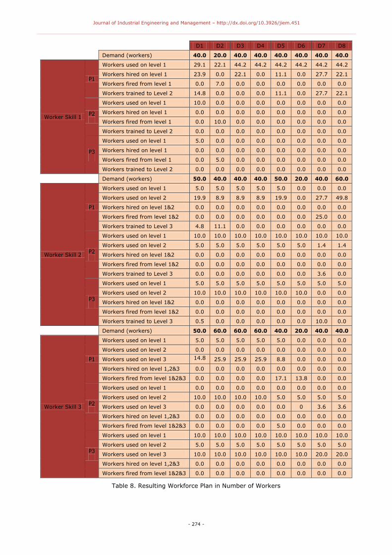
Table 8. Resulting Workforce Plan in Number of Workers


- 275 -

D1 D2 D3 D4 D5 D6 D7 D8

Demand (hours) 320.0 160.0 320.0 320.0 320.0 320.0 320.0 320.0

Worker Skill 1

P1

Regular time on level 1 152.3 115.8 231.6 231.5 231.5 231.5 231.5 231.5

Breaks 1 80.3 61.0 122.0 122.0 122.0 122.0 122.0 120.0

Overtime Hours 58.1 44.2 88.4 88.4 88.4 88.4 88.4 88.4

P2


Breaks 1 27.0 0.0 0.0 0.0 0.0 0.0 0.0 0.0

Overtime Hours 20.0 0.0 0.0 0.0 0.0 0.0 0.0 0.0

P3


Breaks 1 13.3 0.0 0.0 0.0 0.0 0.0 0.0 0.0

Overtime Hours 10.0 0.0 0.0 0.0 0.0 0.0 0.0 0.0

Demand (hours) 400.0 320.0 320.0 320.0 400.0 160.0 320.0 480.0

Worker Skill 2

P1



Breaks 1&2 68.9 38.4 38.4 38.4 68.9 0.0 76.5 137.5

Overtime Hours 49.8 27.8 27.8 27.8 49.8 0.0 55.4 99.6

P2



Breaks 1&2 40.7 40.7 40.7 40.7 40.7 40.7 30.8 30.8

Overtime Hours 30.0 30.0 30.0 30.0 30.0 0.6 22.7 22.7

P3



Breaks 1&2 39.8 39.8 39.8 39.8 39.8 39.8 13.3 13.3

Overtime Hours 30.0 30.0 30.0 30.0 30.0 0.0 10.0 10.0

Demand (hours) 400.0 480.0 480.0 480.0 320.0 160.0 320.0 320.0

Worker Skill 3

P1




Breaks 1&2&3 54.8 85.3 85.3 85.3 38.1 0.0 0.0 0.0

Overtime Hours 39.6 61.7 61.7 61.7 27.6 0.0 0.0 0.0

P2




Breaks 1&2&3 27.2 27.2 27.2 27.2 13.6 13.6 23.5 23.5

Overtime Hours 20.0 20.0 20.0 20.0 10.0 0.0 17.3 17.3

P3




Breaks 1&2&3 66.4 66.4 66.4 66.4 66.4 66.4 128.9 86.9

Overtime Hours 50.0 50.0 50.0 50.0 50.0 0.0 70.0 70.0

Table 9. Resulting Workforce Plan in Worker-hours

This research shows that workers’ differences can be used to predict hiring, firing and training

workers and total break time. Table 8 shows the number of workers hired, fired and trained in

each period for different personality levels. Also, Table 9 shows the time workers spend on all

the tasks to satisfy the demand and the amount of break they take due to the fatigue level for

each worker. From Tables 8 and 9, it can be seen that the workers who are not working during

regular time have no breaks. Also, we can notice from running the model with different

objectives that a worker at higher personality level required less amount of break to recover

than a worker with low personality level. Moreover, the most of the workers hired and trained

have low personality level, which represents the normal scenario in practice since it is assumed


- 276 -

the lower personality levels workers costs less than workers with high personality levels.

However, these results will be different if the input data are changed or when the company

goals are changed, as shown in Table 10. For example, if we considered different productivities

for different workers personality levels, the model will prefer to hire and use workers with

higher personality levels because of their high performance.

4.2. Model implementation and results analysis

All workers have the right to take breaks. The actual amount of break a worker receives is

usually set out in his contract of employment. Although there are some kinds of jobs that do

not allow workers to take breaks such as air or sea transport and working part time during

busy peak periods, not taking a break can result in overloaded, stressed, and unproductive

workers. Rest breaks are one of break types that workers can take under special rules written

in the employment contact. This model can help to estimate the amount of break a worker can

take during a working day in order to minimize the risk caused by worker fatigue. In the

previous section, a simple numerical example is given to illustrate the performance of the

model. In this section, we will study the effects of fatigue level and worker differences on

workforce decisions. Table 10 shows a comparison between the two cases with different goals.

Also, it shows a comparison between two cases; the first one represents the case where

fatigue level is different and the second one represents the case where the fatigue level is the

same. However, considering human differences that exist between workers results in more

accurate workforce decisions. In Table 10, it is assumed that the fractions of maximum

workers’ capability are set to be the average values. This fraction can be used to determine the

values of maximum endurance time, recovery rate and maximum fatigue. Also, it is assumed

that we decision maker is looking to achieve three goals; costs minimization, the number of

top performers fired minimization and idle time minimization.

Total Goal 1 Goal 2 Goal 3 Goal 4 Equal weights

(Different fatigue)

Equal weights

(Same fatigue)

Objective Value 223,618.2 1.9 2846.6 0.0 0.05 0.03

Demand (Wd.days) 8,080.0 8,080.0 8,080.0 8,080.0 8,080.0 8,080.0

Regular Time (hrs) 6,270.8 7,883.5 5,894.5 8,080 5,967.5 5,962.3

Overtime (hrs) 1,810.223 206.0 2,185.3 0.0 2,112.5 2,117.6

Breaks (W.hrs) 3,295.5 3,957.5 2,846.5 4,021 2,955.2 2,984.1

Workers (W.days) 1,195.7 1,478.9 1092.7 1,512.6 1,115.3 1,118.3

Training (W.days) 77.2 21.8 82.9 54.9 101.4 115.9

Hiring (W.days) 70.4 265.5 249.5 344.8 104.9 105.8

Firing (W.days) 46.9 186.6 227.9 264.7 82.5 82.6

Fatigue (%.hr) 68.4 45.3 76.3 0.0 72.9 83.9

Costs ($) 223,618.2 273,341.2 286,859.8 304,191.0 229,798.0 230,056.5 d W represents Worker

Table 10. Comparisons Between the Different Goals


- 277 -

This table shows the comparisons between the two cases regarding the importance of

considering fatigue level differences between workers to generate a better solution. The total

cost when fatigue level is same for all workers is $230,056.5, but when we consider different

fatigue level between workers, the total cost is $229,798.0. The results show that by

considering worker differences in the model the costs differences are not significant. Also, the

present study found that fatigue is not significantly important for scheduling day workers from

the economics perspective, but it help to determine the amount of the break workers can take

depending on his personality, and salaries profiles. Further research should be done on the

effects of the fatigue on worker scheduling with different shifts. Moreover, if the initial number

of workers is changed, the number of hired, fired or trained workers is changed which will

change the total costs. Also, in Table 9, we can notice that the company can use this model in

planning process by selecting the specific goals based on its policy and budget. For example,

we can assign a target value for each goal so that we can determine the number of workers

needed in each period to satisfy the demand without exceeding the predefined goals.

4.3. Sensitivity Analysis

Realistic mixed integer programming models require large amounts of data. Accurate data are

expensive to collect, so we will generally be forced to use data in which we have less than

complete confidence. This section discusses the actual implementation of the proposed model

by manipulating different alternatives and analyzing the sensitivity of decision parameters to

the variation of relevant conditions, based on the preceding numerical example.

4.3.1 Implications Regarding Different Model Goals

A user of a model should be concerned with how the recommendations of the model are

altered by changes in the input data. Table 11 illustrates the comparisons between different

scenario problems and the effects of changing the weights of the company goals on the total

costs and utilization of the work. In this Table, we implement 10 scenarios to compare

between the final results in terms of workers’ utilization, workers’ fatigue, and the total costs.

The worker utilization is calculated by dividing the total productive time for all the workers by

the total available hours. Worker break percentages represent the amount of break workers

can take in average during a working day. Also, workers' fatigue represents the total physical

load on the workforce during a working day. We change each scenario by changing the weights

of the unwanted deviational variables in the objective function to show its effects on the final

objective value. For example, in scenario 1, all goals have the same importance in the

objective function.

In the weighted goal programming method, we can use a set of preference weights assigned to

the penalisation of unwanted deviations to provide solutions that are of practical use to the

problem owner. In this weight space analysis, it is assumed that all weighting vectors have

been normalized and hence sum to one. Note that in practice the weight of an unwanted


- 278 -

deviational variable has to be greater than zero to avoid the possibility of generating Pareto-

inefficient solutions. Tamiz and Jones (1996) defined Pareto inefficiency as an objective that

can be improved without worsening the value of any other objective. Therefore, a small weight

(e.g. 0.005) is suggested to replace a zero weight. Heuristic method and sensitivity analysis

are developed to find the weight values in the weighting space (Jones & Tamiz, 2010). By

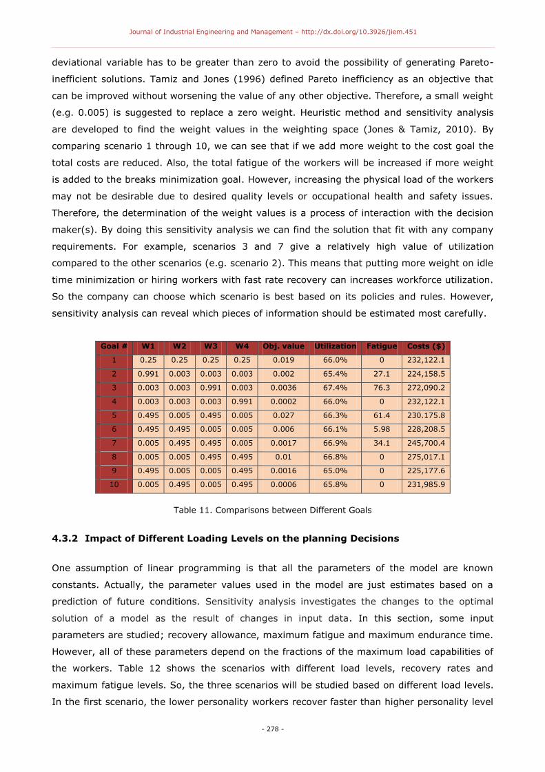
comparing scenario 1 through 10, we can see that if we add more weight to the cost goal the

total costs are reduced. Also, the total fatigue of the workers will be increased if more weight

is added to the breaks minimization goal. However, increasing the physical load of the workers

may not be desirable due to desired quality levels or occupational health and safety issues.

Therefore, the determination of the weight values is a process of interaction with the decision

maker(s). By doing this sensitivity analysis we can find the solution that fit with any company

requirements. For example, scenarios 3 and 7 give a relatively high value of utilization

compared to the other scenarios (e.g. scenario 2). This means that putting more weight on idle

time minimization or hiring workers with fast rate recovery can increases workforce utilization.

So the company can choose which scenario is best based on its policies and rules. However,

sensitivity analysis can reveal which pieces of information should be estimated most carefully.

Goal # W1 W2 W3 W4 Obj. value Utilization Fatigue Costs ($)

1 0.25 0.25 0.25 0.25 0.019 66.0% 0 232,122.1

2 0.991 0.003 0.003 0.003 0.002 65.4% 27.1 224,158.5

3 0.003 0.003 0.991 0.003 0.0036 67.4% 76.3 272,090.2

4 0.003 0.003 0.003 0.991 0.0002 66.0% 0 232,122.1

5 0.495 0.005 0.495 0.005 0.027 66.3% 61.4 230.175.8

6 0.495 0.495 0.005 0.005 0.006 66.1% 5.98 228,208.5

7 0.005 0.495 0.495 0.005 0.0017 66.9% 34.1 245,700.4

8 0.005 0.005 0.495 0.495 0.01 66.8% 0 275,017.1

9 0.495 0.005 0.005 0.495 0.0016 65.0% 0 225,177.6

10 0.005 0.495 0.005 0.495 0.0006 65.8% 0 231,985.9

Table 11. Comparisons between Different Goals

4.3.2 Impact of Different Loading Levels on the planning Decisions

One assumption of linear programming is that all the parameters of the model are known

constants. Actually, the parameter values used in the model are just estimates based on a

prediction of future conditions. Sensitivity analysis investigates the changes to the optimal

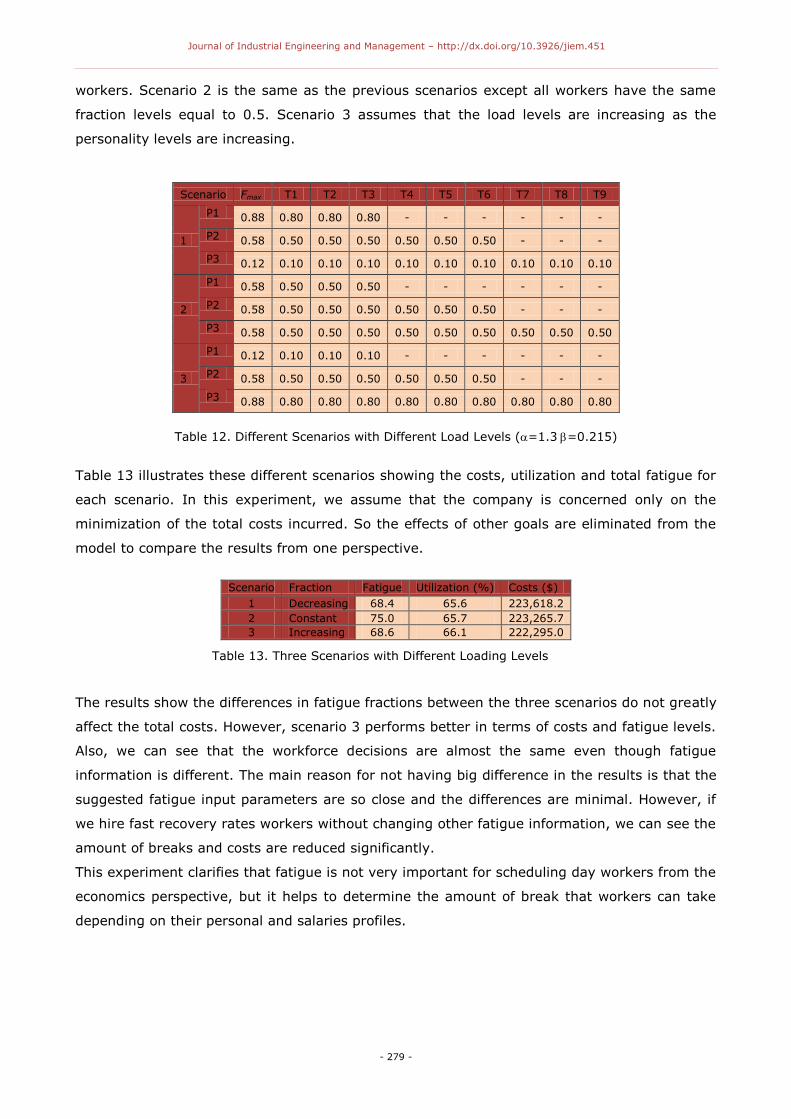
solution of a model as the result of changes in input data. In this section, some input

parameters are studied; recovery allowance, maximum fatigue and maximum endurance time.

However, all of these parameters depend on the fractions of the maximum load capabilities of

the workers. Table 12 shows the scenarios with different load levels, recovery rates and

maximum fatigue levels. So, the three scenarios will be studied based on different load levels.

In the first scenario, the lower personality workers recover faster than higher personality level


- 279 -

workers. Scenario 2 is the same as the previous scenarios except all workers have the same

fraction levels equal to 0.5. Scenario 3 assumes that the load levels are increasing as the

personality levels are increasing.

Scenario Fmax

T1 T2 T3 T4 T5 T6 T7 T8 T9

1

P1 0.88 0.80 0.80 0.80 - - - - - -

P2 0.58 0.50 0.50 0.50 0.50 0.50 0.50 - - -

P3 0.12 0.10 0.10 0.10 0.10 0.10 0.10 0.10 0.10 0.10

2

P1 0.58 0.50 0.50 0.50 - - - - - -

P2 0.58 0.50 0.50 0.50 0.50 0.50 0.50 - - -

P3 0.58 0.50 0.50 0.50 0.50 0.50 0.50 0.50 0.50 0.50

3

P1 0.12 0.10 0.10 0.10 - - - - - -

P2 0.58 0.50 0.50 0.50 0.50 0.50 0.50 - - -

P3 0.88 0.80 0.80 0.80 0.80 0.80 0.80 0.80 0.80 0.80

Table 12. Different Scenarios with Different Load Levels (=1.3=0.215)

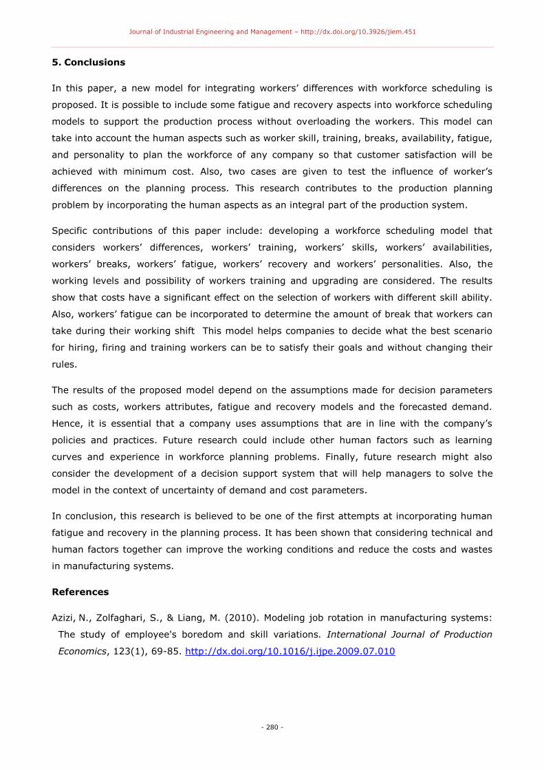
Table 13 illustrates these different scenarios showing the costs, utilization and total fatigue for

each scenario. In this experiment, we assume that the company is concerned only on the

minimization of the total costs incurred. So the effects of other goals are eliminated from the

model to compare the results from one perspective.

Scenario Fraction Fatigue Utilization (%) Costs ($)

1 Decreasing 68.4 65.6 223,618.2

2 Constant 75.0 65.7 223,265.7

3 Increasing 68.6 66.1 222,295.0

Table 13. Three Scenarios with Different Loading Levels

The results show the differences in fatigue fractions between the three scenarios do not greatly

affect the total costs. However, scenario 3 performs better in terms of costs and fatigue levels.

Also, we can see that the workforce decisions are almost the same even though fatigue

information is different. The main reason for not having big difference in the results is that the

suggested fatigue input parameters are so close and the differences are minimal. However, if

we hire fast recovery rates workers without changing other fatigue information, we can see the

amount of breaks and costs are reduced significantly.

This experiment clarifies that fatigue is not very important for scheduling day workers from the

economics perspective, but it helps to determine the amount of break that workers can take

depending on their personal and salaries profiles.


- 280 -

5. Conclusions

In this paper, a new model for integrating workers’ differences with workforce scheduling is

proposed. It is possible to include some fatigue and recovery aspects into workforce scheduling

models to support the production process without overloading the workers. This model can

take into account the human aspects such as worker skill, training, breaks, availability, fatigue,

and personality to plan the workforce of any company so that customer satisfaction will be

achieved with minimum cost. Also, two cases are given to test the influence of worker’s

differences on the planning process. This research contributes to the production planning

problem by incorporating the human aspects as an integral part of the production system.

Specific contributions of this paper include: developing a workforce scheduling model that

considers workers’ differences, workers’ training, workers’ skills, workers’ availabilities,

workers’ breaks, workers’ fatigue, workers’ recovery and workers’ personalities. Also, the

working levels and possibility of workers training and upgrading are considered. The results

show that costs have a significant effect on the selection of workers with different skill ability.

Also, workers’ fatigue can be incorporated to determine the amount of break that workers can

take during their working shift This model helps companies to decide what the best scenario

for hiring, firing and training workers can be to satisfy their goals and without changing their

rules.

The results of the proposed model depend on the assumptions made for decision parameters

such as costs, workers attributes, fatigue and recovery models and the forecasted demand.

Hence, it is essential that a company uses assumptions that are in line with the company’s

policies and practices. Future research could include other human factors such as learning

curves and experience in workforce planning problems. Finally, future research might also

consider the development of a decision support system that will help managers to solve the

model in the context of uncertainty of demand and cost parameters.

In conclusion, this research is believed to be one of the first attempts at incorporating human

fatigue and recovery in the planning process. It has been shown that considering technical and

human factors together can improve the working conditions and reduce the costs and wastes

in manufacturing systems.

References

Azizi, N., Zolfaghari, S., & Liang, M. (2010). Modeling job rotation in manufacturing systems:

The study of employee's boredom and skill variations. International Journal of Production

Economics, 123(1), 69-85. http://dx.doi.org/10.1016/j.ijpe.2009.07.010

http://dx.doi.org/10.1016/j.ijpe.2009.07.010


- 281 -

Berglund, M., & Karltun, J. (2007). Human, technological and organizational aspects

influencing the production scheduling process. International Journal of Production Economics,

110(1-2), 160–174. http://dx.doi.org/10.1016/j.ijpe.2007.02.024

Bidanda, B., Ariyawonggrat, P., Needy, K.L., Norman, B.A., & Tharmmaphornphilas, W.

(2005). Human related issues in manufacturing cell design, implementation, and operation: a

review and survey. Computers & Industrial Engineering, 48(3), 507–523.

http://dx.doi.org/10.1016/j.cie.2003.03.002

Birch, S., O’Brien-Pallas, L., Alksnis, C., Tomblin Murphy, G., & Thomson D. (2003). Beyond

demographic change in human resources planning: an extended framework and application

to nursing. Journal of Health Services Research and Policy, 8(4), 225-229.

http://dx.doi.org/10.1258/135581903322403290

Blumberg, M., & Pringle, C.D. (1982). The missing opportunity in organizational research:

some implications for a theory of work performance. Academy of Management Review, 7(4),

560–569.

Butler, M.P. (2003). Corporate ergonomics programme at Scottish & Newcastle. Applied

Ergonomics, 34(1), 35–38. http://dx.doi.org/10.1016/S0003-6870(02)00082-0

Buzacott, J.A. (2002). The impact of worker differences on production system output.

International Journal of Production Economics, 78(1), 37–44.

http://dx.doi.org/10.1016/S0925-5273(00)00086-4

Castley, R.J. (1996). Policy-focused approach to manpower planning. International Journal of

Manpower, 17(3), 15-24. http://dx.doi.org/10.1108/01437729610119487

Cohon, J.L. (1978). Multiobjective programming and planning, New York: Academic Press

Corominas, A, Olivella, J., & Pastor, R. (2010). A model for assignment of a set of tasks when

work performance depends on experience of all tasks involved. International Journal of

Production Economics, 126(2), 335–340. http://dx.doi.org/10.1016/j.ijpe.2010.04.012

Da Silva, C.G, Figueira, J., Lisboa, J., & Barman, S. (2006). An interactive decision support

system for an aggregate production planning model based on multiple criteria mixed integer

linear programming. The International Journal of Management Science, 34(2), 167–177.

http://dx.doi.org/10.1016/j.omega.2004.08.007

De Kluyver, C.A. (1979). An exploration of various goal programming formulations-with

application to advertising media scheduling. Journal of the Operational Research Society,

30(2),167-171

http://0-www.sciencedirect.com.mercury.concordia.ca/science?_ob=ArticleURL&_udi=B6V1W-4TCGM6F-1&_user=1069146&_coverDate=07%2F31%2F2009&_alid=1106316825&_rdoc=1&_fmt=full&_orig=search&_cdi=5685&_st=12&_docanchor=&view=c&_ct=5&_acct=C000051262&_version=1&_urlVersion=0&_userid=1069146&md5=0347c43756ea5e5c4b8727f757bbcd27#bbib39



http://dx.doi.org/10.1258/135581903322403290

http://dx.doi.org/10.1016/S0003-6870(02)00082-0

http://dx.doi.org/10.1016/S0925-5273(00)00086-4

http://dx.doi.org/10.1108/01437729610119487


http://dx.doi.org/10.1016/j.omega.2004.08.007


- 282 -

Dul, J., & Neumann, W.P. (2009). Ergonomics contributions to company strategies. Applied

Ergonomics, 40(4), 745-752. http://dx.doi.org/10.1016/j.apergo.2008.07.001

Eklund, J. (1997). Ergonomics, quality and continuous improvement – conceptual and

empirical relationships in an industrial context. Ergonomics, 40(10), 982-1001.

Felan, J.T., & Fry, T.D. (2001). Multi-level heterogeneous worker flexibility in a Dual Resource

Constrained (DRC) job-shop. International Journal of Production Research, 39(14), 3041-

3059. http://dx.doi.org/10.1080/00207540110047702

Hägg, G.M., (2003). Corporate initiatives in ergonomics – an introduction. Applied Ergonomics,

34(1), 3–15. http://dx.doi.org/10.1016/S0003-6870(02)00078-9

Helander, M. (1999). Seven common reasons to not implement ergonomics. International

Journal of Industrial Ergonomics, 25(1), 97–101. http://dx.doi.org/10.1016/S0169-

8141(98)00097-3

Hillier, F.S., & Lieberman, G.J. (2010). Introduction to Operations Research, 9th ed., Burr

Ridge, IL: Irwin/McGraw-Hill.

Jaber, M.Y., & Neumann, W.P. (2010). Modeling worker fatigue and recovery in dual-resource

constrained systems. Computers & Industrial Engineering, 59(1), 75-84.


Jamalnia, A., & Soukhakian, M.A. (2009). A hybrid fuzzy goal programming approach with

different goal priorities to aggregate production planning. Computers & Industrial

Engineering, 56(4), 1474-1486. http://dx.doi.org/10.1016/j.cie.2008.09.010

Jenkins, S., & Rickards, J. (2001). The economics of ergonomics: Three workplace design case

studies. In: D.C. Alexander & R. Rabourn (Eds.), Applied ergonomics (pp.238-243), London:

Taylor & Francis.

Jensen P.L. (2002). Human factors and ergonomics in the planning of production. International

Journal of Industrial Ergonomics, 29(3), 121–131. http://dx.doi.org/10.1016/S0169-

8141(01)00056-7

Jones, D., & Tamiz, M. (2010). Practical goal programming. (1st ed.). New York, London:

Springer

Jones, D.F. (1995). The design and development of an intelligent goal programming system.

PhD. Thesis. University of Portsmouth, UK.

Masud, A.S., & Hwang, C.L. (1981). Interactive sequential goal programming. Journal of the

Operational Research Society, 32(5), 391-400.

http://dx.doi.org/10.1016/j.apergo.2008.07.001

http://dx.doi.org/10.1080/00207540110047702

http://dx.doi.org/10.1016/S0003-6870(02)00078-9

http://dx.doi.org/10.1016/S0169-8141(98)00097-3

http://dx.doi.org/10.1016/S0169-8141(98)00097-3



http://0-www.sciencedirect.com.mercury.concordia.ca/science?_ob=ArticleURL&_udi=B6V27-4TG9HPV-1&_user=1069146&_coverDate=05%2F31%2F2009&_alid=1222286503&_rdoc=3&_fmt=high&_orig=search&_cdi=5695&_sort=r&_docanchor=&view=c&_ct=39304&_acct=C000051262&_version=1&_urlVersion=0&_userid=1069146&md5=fe09daeac6fe1f397d0f4af26aed412b#hit3


http://dx.doi.org/10.1016/S0169-8141(01)00056-7

http://dx.doi.org/10.1016/S0169-8141(01)00056-7


- 283 -

Neumann, W.P., & Medbo, P. (2009). Integrating human factors into discrete event simulations

of parallel flow strategies. Production Planning and Control, 20(1), 3-16.

http://dx.doi.org/10.1080/09537280802601444

Oxenburgh, M., Marlow, P., & Oxenburgh, A. (2004). Increasing productivity and profit through

health and safety: The financial returns from a safe working environment (2nd Ed.). Boca

Raton, Florida: CRC Press.

Perrow, C. (1983). The organizational context of human factor engineering. Administrative

Science Quarterly, 28(4), 521–541.

Siebers, P.O. (2004). The impact of human performance variation on the accuracy of

manufacturing system simulation models, PhD thesis, Cranfield University, School of

Industrial and Manufacturing Science, UK.

Siebers, P.O. (2006). Worker performance modeling in manufacturing systems simulation. In

Rennard, J.-P., (Ed.). Handbook of research on nature inspired computing for economy and

management (pp. 661-678). Pennsylvania: Idea Group Publishing.

Stewart, B.D., Webster, D.B., Ahmad, S., & Matson J.O. (1994). Mathematical models for

developing a flexible workforce. International Journal of Production Economics, 36(3), 243-

254. http://dx.doi.org/10.1016/0925-5273(94)00033-6

Tamiz, M., & Jones, D.F. (1996). Goal programming and Pareto efficiency. Journal of

Information and Optimization Sciences , 17(2), 291-3Tamiz, M., Jones, D., & Romero, C.

(1998). Goal programming for decision making: An overview of current state-of-the-art.

European Journal of Operational Research, 111(3), 569-581

Torabi S.A., Ebadian M., & Tanha R. (2010). Fuzzy hierarchical production planning (with a

case study). Fuzzy Sets and Systems, 161(11), 1511–1529.

http://dx.doi.org/10.1016/j.fss.2009.11.006

Udo, G.G., & Ebiefung, A.A. (1999). Human factors affecting the success of advanced

manufacturing systems. Computers & Industrial Engineering, 37(1-2), 297–300.

http://dx.doi.org/10.1016/S0360-8352(99)00078-9

Widhelm, W.B. (1981). Extensions of goal programming models. The International Journal of

Management Science, 9(2), 212-214

Wilson, J.R. (2000). Fundamentals of ergonomics in theory and practice. Applied Ergonomics,

31(6), 557-567. http://dx.doi.org/10.1016/S0003-6870(00)00034-X

http://dx.doi.org/10.1080/09537280802601444

http://www.sciencedirect.com/science?_ob=ArticleURL&_udi=B6V31-444233M-1&_user=1069146&_coverDate=03%2F31%2F2002&_alid=1162278350&_rdoc=1&_fmt=high&_orig=search&_cdi=5717&_sort=r&_st=4&_docanchor=&_ct=67592&_acct=C000051262&_version=1&_urlVersion=0&_userid=1069146&md5=c9723243c952d0d97c86faa30d1272d0#bbib30

http://dx.doi.org/10.1016/0925-5273(94)00033-6

http://dx.doi.org/10.1016/j.fss.2009.11.006

http://dx.doi.org/10.1016/S0360-8352(99)00078-9

http://dx.doi.org/10.1016/S0003-6870(00)00034-X


- 284 -

Wirojanagud, P., Gel, E.S., Fowler, J.W., & Cardy, R. (2007). Modeling inherent worker

differences for workforce planning. International Journal of Production Research, 45(3), 525–

553. http://dx.doi.org/10.1080/00207540600792242

Journal of Industrial Engineering and Management, 2012 (www.jiem.org)

El artículo está con Reconocimiento-NoComercial 3.0 de Creative Commons. Puede copiarlo, distribuirlo y comunicarlo públicamente

siempre que cite a su autor y a Intangible Capital. No lo utilice para fines comerciales. La licencia completa se puede consultar en

http://creativecommons.org/licenses/by-nc/3.0/es/

http://dx.doi.org/10.1080/00207540600792242

http://www.intangiblecapital.org/





Workforce scheduling: A new model incorporating human factors

Documents

Transcript of Workforce scheduling: A new model incorporating human factors