Workforce Investment Act (WIA) Net Impact Estimates and Rates of Return

Kevin Hollenbeck

November 7, 2009

W.E. Upjohn Institute for Employment Research 300 S. Westnedge Ave. Kalamazoo, MI 49007

hollenbeck@upjohninstitute.org

Paper to be presented at the European Commission-sponsored meeting titled, “What the European Social Fund Can Learn from the WIA Experience” in Washington, DC. This paper builds on work that was done under contract to the Workforce Education and Training Board of the State of Washington, the Senior Advisor’s Office of the Commonwealth of Virginia, and the Indiana Chamber of Commerce Foundation. The contractual support of and provision of administrative data by these three states as well as the resources and support of the Upjohn Institute are gratefully acknowledged. Wei-Jang Huang provided invaluable research assistance. The usual caveat applies.

ABSTRACT The net impacts and private and social benefits and costs of workforce development

programs were estimated in four separate studies; two of them examining programs in Washington, one in Virginia, and one in Indiana. The programs included the public job training system, programs at community and technical colleges, adult basic education, private career schools, high school career and technical education, and vocational rehabilitation for disabled individuals and for blind or visually impaired individuals. This paper will focus on the programs offered by the public job training system (administered and funded by the Workforce Investment Act (WIA) and its predecessor act, the Job Training Partnership Act (JTPA)).

The net impact analyses were conducted using a nonexperimental methodology. Individuals who had encountered the workforce development programs were statistically matched to individuals who had not. Administrative data with information from the universe of program participants and Labor Exchange data for registrants (who served as the comparison group pool) were used for the analyses. These data included several years of pre-program and outcome information including demographics, employment and earnings information from the Unemployment Insurance wage record system, and transfer income information such as Food Stamps and Temporary Assistance for Needy Families (TANF) recipiency and benefits.

This paper presents the results from the studies and extends them in three directions. First, it compares and contrasts the results across the four studies. Second, two studies present a decomposition of the net impacts into employment, wage, and hours impacts. Third, it displays rates of return for individuals served by the programs, for state taxpayers, and for society as a whole. In general, we find positive net impacts and returns on investment for virtually all of the programs.

The policy implications of this work are several in number. First, the studies add to the

inventory of work that demonstrates that useful evaluations of workforce development education and training programs can be done with administrative data. Second, the decomposition of net earnings impacts into employment, hours, and wage rates adds rich understanding to the impacts of these programs. The rate of return analyses demonstrate that the public (i.e., taxpayers) and society as a whole can benefit financially from public training investments, although the payoffs generally take more than 10 quarters to offset the costs.

Finally, the results for individual programs are illuminating. The estimates presented

here suggest that the Workforce Investment Act services for adults seem to have a significant positive impact on employment, wage rates, and earnings. Not surprisingly, the analyses point out the large foregone earnings that are borne by dislocated workers during their training that dampen the financial payoff to training. Policy makers may wish to consider stronger support mechanisms for these workers such as stipends during training.

1

INTRODUCTION

This paper contrasts and compares the net impacts of workforce development programs

estimated in four independent studies done in three states. These estimates were computed using

a nonexperimental methodology in which individuals who had been served by the workforce

system in the state were statistically matched to individuals who had encountered the

Employment Service. The impetus for these studies was a commitment on the part of these

states to public accountability and data-driven performance monitoring and management.

In three of the studies from which the net impacts that are reported here emanate, rates of

return have been calculated for the workforce development programs that include a full

accounting of the opportunity costs of participants’ training investments, tax liabilities incurred

due to increased earnings, as well as changes in earnings-conditioned transfers such as

unemployment compensation, TANF benefits, food stamps, and Medicaid. Furthermore these

two studies estimate the net impacts on earnings as well as the components of earnings:

employment, hours, and wage rates.

The contributions of this paper are fourfold: 1) to compare and contrast the net impacts

on employment and earnings across the three independent studies; 2) to show the decomposition

of the net impacts into employment rates, hours, and wage rates; 3) to present rates of return to

individuals, states, and society, and 4) to point out policy implications of the work.

The next section of the paper will provide detail about the programs that were examined

in these studies, the specific outcomes for which net impact estimates were generated, and the

analysis periods. All four studies used administrative data from multiple workforce development

programs, but this paper will focus on the programs offered by the public job training system

(administered and funded by the Workforce Investment Act (WIA) and its predecessor act, the

2

Job Training Partnership Act (JTPA)). The succeeding section of the paper will present the

results of the studies for those programs -- net impacts and rates of return. Next, we discuss

briefly how the net impact and rates of return estimates compare to other studies in the literature.

The final section presents some policy implications of the work.

PROGRAMS, OUTCOMES, AND TIME PERIODS

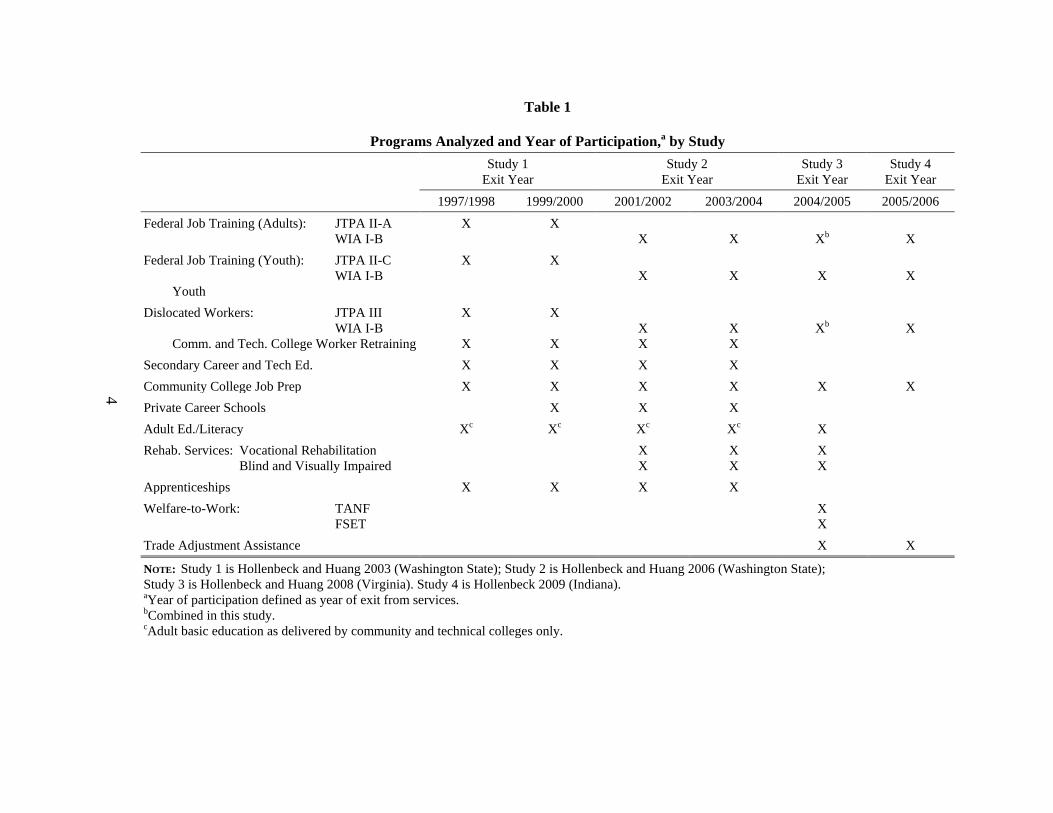
This paper draws from four studies. Each study examined a slightly different set of

workforce development programs covering different time periods. Table 1 displays the various

programs and time periods. The first two studies, done in Washington, focused on

approximately the same programs: federal job training for adults, dislocated workers, and youth;

a state-supported program for dislocated workers; apprenticeships; and four types of educational

programs: adult basic education, high school career and technical education, community college

job prep, and private career schools. In the second study in Washington, rehabilitative services

programs were added to the scope of work. The programs analyzed for the study done in

Virginia overlapped these programs somewhat: they included the federal job training programs

for adults, dislocated workers, and youth; community college career and technical education;

adult education; and rehabilitative services. In addition, this study included trade adjustment

assistance, welfare-to-work, and Food Stamps Employment and Training (FSET). In Indiana,

we estimated the net impacts of the federal job training programs for adults, dislocated workers,

and youth; community college career and technical education; and trade adjustment assistance.

As noted in table 1, the time periods in which the participants were in the programs

varied across the studies. The studies defined participation year by when the individual exited

from the program. All of the studies used the entire universe of program exiters: in 1997/98 and

1999/00 for the first Washington study; in 2001/02 and 2003/04 for the second Washington

3

study; 2004/05 for the Virginia study; and 2005/06 for Indiana. To be clear, someone who

participated in a program for three years and who exited sometime during 1997/98 is considered

to be a 1997/98 participant, as is someone who both entered and exited in 1997/98.1

In all studies, the net impacts of participation in the workforce development programs on

employment and earnings were estimated. The data came from the quarterly wage record data

generated from the Unemployment Insurance (UI) system, and thus are measured over a calendar

quarter. In Washington, the wage record data include hours worked in a quarter, so for the

studies undertaken for that state, we estimated the net impacts on hours worked per quarter and

hourly wages. Virginia had an interest in the extent to which participants earned credentials

either during program participation or within a year of exit, so that outcome was analyzed in the

Virginia study.

2

The Washington studies also examined the net impact of program participation on the

receipt of unemployment compensation benefits, public assistance benefits (TANF and Food

Stamps), and Medicaid enrollment. These data were supplied by the state agencies that

administer those programs. Table 2 summarizes the outcomes that were examined in the studies.

As table 2 notes, all of the studies focused on two outcome time periods: a short-term outcome

and a longer-term outcome. In Washington, these were three full quarters after exit and 8-11 full

The Indiana study focused on employment and earnings as well as post-training

unemployment compensation benefits.

1 In the terminology of Imbens and Angrist (1994), the estimates that we have produced are local average

treatment effects (LATE). If we had used entry date to define participation (and matched on it rather than exit date), then we would be estimating the average treatment effect (ATE). In general, the former are larger than the latter.

2The Virginia study also used the wage record data to develop an outcome variable that was used to measure employer satisfaction.

4

Table 1

Programs Analyzed and Year of Participation,a by Study

Study 1 Exit Year

Study 2 Exit Year

Study 3 Exit Year

Study 4 Exit Year

1997/1998 1999/2000 2001/2002 2003/2004 2004/2005 2005/2006

Federal Job Training (Adults): JTPA II-A WIA I-B

X X X

X

Xb

X

Federal Job Training (Youth): JTPA II-C WIA I-B Youth

X X X

X

X

X

Dislocated Workers: JTPA III WIA I-B Comm. and Tech. College Worker Retraining

X

X

X

X

X X

X X

Xb

X

Secondary Career and Tech Ed. X X X X Community College Job Prep X X X X X X Private Career Schools X X X Adult Ed./Literacy Xc Xc Xc Xc X Rehab. Services: Vocational Rehabilitation

Blind and Visually Impaired X

X X X

X X

Apprenticeships X X X X Welfare-to-Work: TANF

FSET X

X

Trade Adjustment Assistance X X

NOTE: Study 1 is Hollenbeck and Huang 2003 (Washington State); Study 2 is Hollenbeck and Huang 2006 (Washington State); Study 3 is Hollenbeck and Huang 2008 (Virginia). Study 4 is Hollenbeck 2009 (Indiana). aYear of participation defined as year of exit from services. bCombined in this study. cAdult basic education as delivered by community and technical colleges only.

5

Table 2

Outcomes Examined and Time Periods, by Study Outcomes Study 1 and Study 2 Study 3 Study 4

Employment Defined as > $100 in a quarter Defined as > $50 in a quarter or enrolled in school if < 18

Defined as > $100 in a quarter; > $50 in a quarter (youth)

Earnings Quarterly earnings totaled across all employers

Quarterly earnings totaled across all employers

Quarterly earnings totaled across all employers

Hours Worked per Quarter Hours totaled across all employers Not available Not available Hourly wages Earnings divided by hours worked Not available Not available Credential completion Not available Credential earned while in program or

within 12 months of exit Not available

Unemployment compensation

Benefits of at least $1 in quarter Not available Benefits of at least $1 in quarter

TANF/Food Stamp benefits Benefits received by assistance unit that included participant of at least $1 in quarter

Not available Not available

Medicaid eligibility State Medicaid administrative data indicated participant was “enrollee” during at least one day in quarter

Not available Not available

Time Periods: Short term Long term

3 full quarters after exit 8–11 full quarters after exit in study 1;

9—12 full quarters after exit in study 2

2 full quarters after exit 4 full quarters after exit

3 full quarters after exit 7 full quarters after exit

NOTE: Study 1 is Hollenbeck and Huang 2003 (Washington State); Study 2 is Hollenbeck and Huang 2006 (Washington State); Study 3 is Hollenbeck and Huang 2008 (Virginia); Study 4 is Hollenbeck 2009 (Indiana).

6

quarters after exit in the first study (9-12 full quarters in the second study). In Virginia, these

were two and four full quarters after exit, respectively, and in Indiana, they were three and seven

full quarters after exit.

SUMMARY OF RESULTS

Net impacts. Table 3 provides a summary of the short-term net impacts of the programs

on employment rates, quarterly hours of employment, average wage rates, and quarterly average

earnings. All of the results in the table for studies 1, 2, and 4 are regression-adjusted, and all of

the outcomes,except for quarterly hours, include zero values.3

Table 3

For the study 3 results, the

employment rates are differences in means and the quarterly earnings results are differences in

Short-Term Net Impact Estimates for WIA (or JTPA)

Program Study

Outcome Employment

Rate Quarterly

Hours Wage Rateb

Quarterly Earningsb

Federal Job Training (Adults) JTPA II-A WIA I-B WIA I-B WIA I-B

1 2 3 4

0.109*** 0.097*** 0.034*** 0.148***

23.0** 52.2***

—a —a

$0.77 $1.49***

—a —a

$349*** $711*** $146*** $549***

Federal Job Training (Youth) JTPA II-C WIA I-B Youth WIA I-B Youth WIA I-B Youth

1 2 3 4

0.061*** 0.042**

−0.039** 0.034

−15.3 4.7

—a —a

−$0.47 $0.20

—a —a

−$175** $66 $62 $24

Dislocated Workers JTPA III WIA I-B WIA I-B

1 2 4

0.075*** 0.087*** 0.170***

19.6*** 58.4***

—a

−$0.55 $1.04***

—a

$278*** $784*** $410***

NOTES: Study 1 is Hollenbeck and Huang 2003 (Washington State); Study 2 is Hollenbeck and Huang 2006 (Washington State); Study 3 is Hollenbeck and Huang 2008 (Virginia); Study 4 is Hollenbeck 2009 (Indiana). *** represents statistical significance at the 0.01 level; ** represents statistical significance at the 0.05 level; * represents statistical significance at the 0.10 level. a Virginia and Indiana wage record data do not include hours so no results for quarterly hours or wage rate. b In $2005/2006.

3 The tables in this paper present results for the entire population. In studies 3 and 4, we have estimated the

net impacts separately by gender as well as for the whole population.

7

non-zero medians between the program participants and matched comparison groups. The wage

rate and earnings impacts are in 2005$. Note that these results include all participants—those

individuals who completed their education or training and those who left without completing.

In examining the first column of data, one can easily discern that most of the programs

have statistically significant positive net impacts on short-term (3 or 4 quarters after exit)

employment rates.4

Table 4 displays the results for longer-term outcomes. These results reflect the extent to

which the short-term impacts are retained. The results are not substantially different from those

in table 3. This suggests that for the most part, the programs’ outcomes do not depreciate during

the first few years after exit. The programs result in a statistically significant positive

employment net impact, and all of them save federal job training for youth, have statistically

significant and positive earnings impacts.

The levels of the impacts are generally in the five to 15 percentage point

range. WIA seems to be generally successful at getting participants employed. The farthest

right column of results shows the net impacts on quarterly earnings (for individuals with

earnings). Whereas the estimates are generally positive, there is more variability in the levels

and statistical significance of the earnings impacts than for employment. For example, the youth

program has earnings impacts that are essentially zero, despite reasonably robust employment

rate impacts.

4 The results for Youth are mixed. The two studies in Washington state show positive and significant

employment gain; but neither the Virginia nor Indiana studies have this result. In fact, the Virginia employment impact for Youth is negative and significant.

8

Table 4

Long-Term Net Impact Estimates of WIA (or JTPA)

Program Study

Outcome Employment

Rate Quarterly

Hours Wage Ratea

Quarterly Earningsa

Federal Job Training (Adults) JTPA II-A WIA I-B WIA I-B

1 2 4

0.074*** 0.066*** 0.137***

23.9*** 35.7***

—b

$0.68** $0.67**

—b

$658*** $455*** $463***

Federal Job Training (Youth) JTPA II-C WIA I-B Youth WIA I-B Youth

1 2 4

0.053** 0.103*** 0.023

2.3

31.1*** —b

−$0.71

$0.77*** —b

$117 $325*** $47

Dislocated Workers JTPA III WIA I-B WIA I-B

1 2 4

0.073*** 0.064*** 0.165***

26.6*** 48.8***

—b

−$0.10

$0.97*** —b

$1,009*** $771*** $310***

NOTES: Study 1 is Hollenbeck and Huang 2003 (Washington State); Study 2 is Hollenbeck and Huang 2006 (Washington State); Study 4 is Hollenbeck (2009). *** represents statistical significance at the 0.01 level; ** represents statistical significance at the 0.05 level; * represents statistical significance at the 0.10 level. a In $2005/2006. b Data not available.

Rates of return. In addition to the net impact analyses, we conducted benefit-cost

analyses for the workforce development programs in the two Washington and in the Indiana

studies. The benefits that were calculated included the following:

• Increased lifetime earnings (discounted) • Fringe benefits associated with those earnings • Taxes on earnings (negative benefit to participants; benefit to society) • Reductions in UI benefits (negative benefit to participants; benefit to society) • Reductions in TANF benefits (negative benefit to participants; benefit to society) • Reductions in Food Stamp benefits (negative benefit to participants; benefit to

society) • Reductions in Medicaid benefits (negative benefit to participants; benefit to

society) The costs included the following:

• Foregone earnings (reduced earnings during the period of training)

9

• Tuition payments • Program costs

Most of these costs and benefits were derived from the net impact estimates. The details about

how these costs and benefits were estimated or calculated are in the appendix.

Table 5 displays the estimated benefits and costs for the JTPA and WIA programs

analyzed in the two Washington studies and for WIA in the Indiana study for the first 10 quarters

after program exit and for the average working lifetime. The table entries represent financial

gains (positive benefits or negative costs) or costs (negative benefits or positive costs) for the

average participant. The costs and benefits are shown from three perspectives: for the

individual, for the public (taxpayers), and for society as a whole. The latter is the sum of the first

two. The dollar figures are in constant $2005/2006 and have been discounted at 3 percent.

The top panel shows that the discounted (net) benefits to the participants over the first 10

quarters after exit are generally in the range of $3,500 to $5,000. The costs to participants are

fairly negligible for the Adults and Youth programs, but they are quite large (in the form of

foregone earnings) for dislocated workers. Concomitantly, the short-term returns on investment

for disadvantaged adult and youth participants in this time period are quite substantial—they are

either positive or incalculable because the costs were non-positive;5

For the public, benefits are generally in the $2,000 to $6,000 range and are typically less

than the public costs of providing services. For almost none of the programs is the rate of return

whereas the return for

dislocated workers is negative in all of the studies.

5 The exception to this is JTPA II-C (Youth). The net impact estimate of loss of TANF benefits is quite

large for this population in Study 1, and this result “drives” the negative benefits

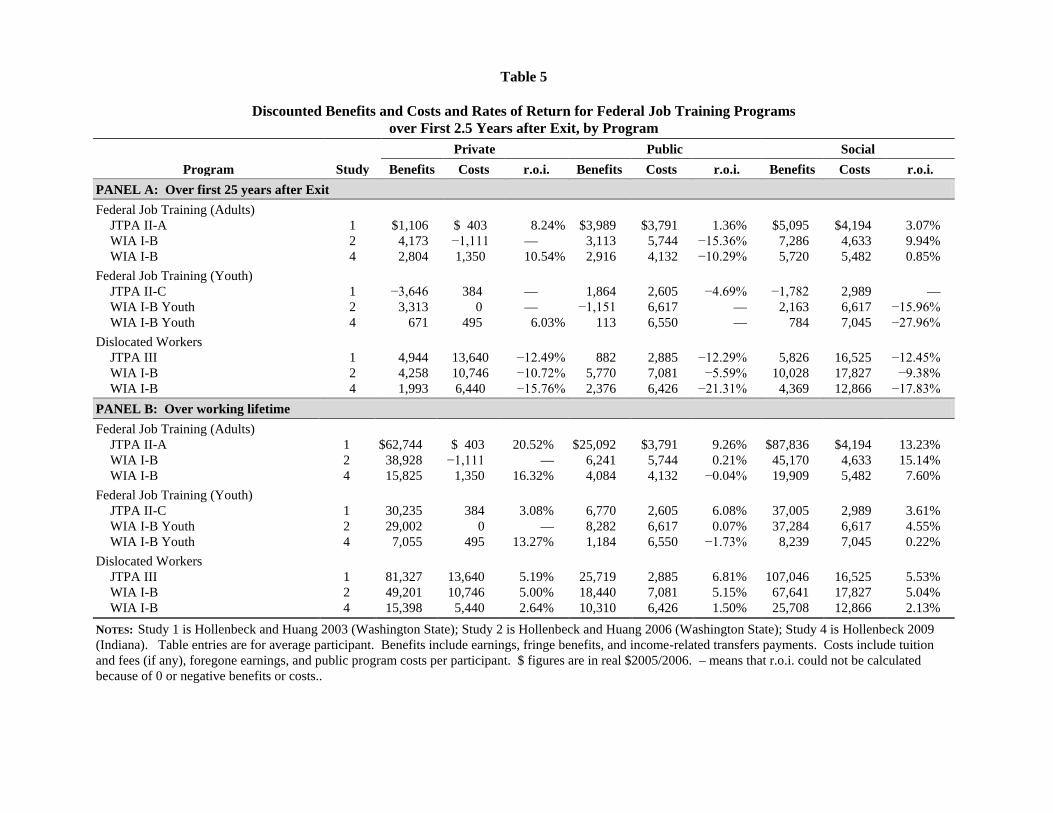
Table 5

Discounted Benefits and Costs and Rates of Return for Federal Job Training Programs over First 2.5 Years after Exit, by Program

Program Study Private Public Social

Benefits Costs r.o.i. Benefits Costs r.o.i. Benefits Costs r.o.i. PANEL A: Over first 25 years after Exit Federal Job Training (Adults) JTPA II-A WIA I-B WIA I-B

1 2 4

$1,106

4,173 2,804

$ 403 −1,111 1,350

8.24%

— 10.54%

$3,989

3,113 2,916

$3,791

5,744 4,132

1.36%

−15.36% −10.29%

$5,095

7,286 5,720

$4,194

4,633 5,482

3.07% 9.94% 0.85%

Federal Job Training (Youth) JTPA II-C WIA I-B Youth WIA I-B Youth

1 2 4

−3,646

3,313 671

384

0 495

— — 6.03%

1,864

−1,151 113

2,605 6,617 6,550

−4.69%

— —

−1,782

2,163 784

2,989 6,617 7,045

—

−15.96% −27.96%

Dislocated Workers JTPA III WIA I-B WIA I-B

1 2 4

4,944 4,258 1,993

13,640 10,746 6,440

−12.49% −10.72% −15.76%

882

5,770 2,376

2,885 7,081 6,426

−12.29%

−5.59% −21.31%

5,826

10,028 4,369

16,525 17,827 12,866

−12.45%

−9.38% −17.83%

PANEL B: Over working lifetime Federal Job Training (Adults) JTPA II-A WIA I-B WIA I-B

1 2 4

$62,744

38,928 15,825

$ 403

−1,111 1,350

20.52%

— 16.32%

$25,092

6,241 4,084

$3,791

5,744 4,132

9.26% 0.21%

−0.04%

$87,836

45,170 19,909

$4,194

4,633 5,482

13.23% 15.14%

7.60% Federal Job Training (Youth) JTPA II-C WIA I-B Youth WIA I-B Youth

1 2 4

30,235 29,002

7,055

384

0 495

3.08%

— 13.27%

6,770 8,282 1,184

2,605 6,617 6,550

6.08% 0.07%

−1.73%

37,005 37,284

8,239

2,989 6,617 7,045

3.61% 4.55% 0.22%

Dislocated Workers JTPA III WIA I-B WIA I-B

1 2 4

81,327 49,201 15,398

13,640 10,746

5,440

5.19% 5.00% 2.64%

25,719 18,440 10,310

2,885 7,081 6,426

6.81% 5.15% 1.50%

107,046

67,641 25,708

16,525 17,827 12,866

5.53% 5.04% 2.13%

NOTES: Study 1 is Hollenbeck and Huang 2003 (Washington State); Study 2 is Hollenbeck and Huang 2006 (Washington State); Study 4 is Hollenbeck 2009 (Indiana). Table entries are for average participant. Benefits include earnings, fringe benefits, and income-related transfers payments. Costs include tuition and fees (if any), foregone earnings, and public program costs per participant. $ figures are in real $2005/2006. – means that r.o.i. could not be calculated because of 0 or negative benefits or costs..

11

for the public positive in the first 10 quarters. This suggests that these programs do not fully

payoff within the first 10 quarters after a participant exits.

Taxes and income-conditioned transfers are transfers between participants and the public,

so they offset each other in the calculation of benefits and costs to society as a whole. Thus the

benefits to society in the cost-benefit analysis are simply the earnings and fringe benefits of

participants, and the costs are the participants’ foregone earnings and the financial cost of

providing the program services. In the first ten quarters, the societal benefits exceed the costs for

the WIA Adult program, but not for Youth or dislocated workers.

The lower panel of the table displays estimated benefits, costs, and return on investments

of the average individual served by a program through their working lifetime. Here we

extrapolated benefits from the average age of exiters until age 65. For individuals, the

discounted (net) lifetime benefits tend to be substantial, especially in the two Washington State

studies. The costs (identical to the costs given in table 5) are much less than these benefits, so

the participants’ returns on investment range from about 2.5% (quarterly) to over 20%

(quarterly).6

Validity. The net impacts and rates of return presented here are, in general, quite

substantial. Are they believable? Does participation in the Workforce Investment Act endow

The benefits accruing to the public over the average worker’s lifetime are

dominated by tax payments on increased earnings. Given that those earnings tend to be quite

substantial, it is not surprising that the public benefits tend to exceed the public costs, and there

tend to be positive returns to the public for the programs. For society, the story is quite similar.

The benefits far exceed the costs, and the returns are therefore quite handsome.

6 Again, two of the returns are not calculable because costs are negative or zero.

12

clients with these sorts of returns? One question that might be raised is the extent to which the

methodological approach is responsible for the positive findings. While it is generally agreed

that a random assignment approach is methodologically superior to the matching estimators used

in the above mentioned studies, it should be noted that the National JTPA Study (NJS) that used

a random assignment process resulted in a 13 percent earnings impact for adult men and a 15

percent earnings impact for adult women according to the U.S. General Accounting Office

(1996). The comparable estimate in table 4--an earnings impact of $658 (2005/2006 $) is about

a 22 percent impact (mean quarterly earnings are $2,946 for this group.) The Washington State

results reported here are larger than the NJS, but both studies imply quite large returns.

Another issue that might be raised is that the author of this paper is also an author of all

of the WIA impact studies cited above. The U.S. Department of Labor funded a quasi-

experimental evaluation of WIA whose results are reported in Heinrich, Mueser, and Troske

(2008). For the WIA adult program, these authors report a significant quarterly earnings impact

of about $600 for women and $450 for men (2005:1 $). The comparable result reported in table

4 is about $450 for the total population. For the WIA dislocated worker program, these authors

report a significant quarterly earnings impact of about $380 for women and $220 for men7

7 Heinrich, Mueser, and Troske (2008) indicate that a difference-in-difference estimate for dislocated

workers attenuates these impacts toward zero.

. The

comparable results reported in table 4 are $771 in Washington State and $310 in Indiana for the

total population. Note that Mueser, Troske, and Gorislavsky (2007) use several quasi-

experimental approaches to estimate the impact of JTPA in the state of Missouri, and their

preferred specification results in an earnings impact of about 14 percent for men and 23 percent

for women. All in all, it seems like the estimates presented here “fit” within the literature.

13

CONCLUSIONS

The contribution of this paper has been to extend in two directions the net impact

estimates that have been generated through nonexperimental methods with administrative data.

In two studies, the net earnings impacts were decomposed into employment, hours of work, and

wage rate impacts. Secondly, the earnings impacts were combined with estimates of impacts on

fringe benefits, tax payments, and income-conditioned transfers to conduct a benefit cost

analysis of workforce programs.

The policy implications of this work are several in number. First, the studies add to the

inventory of work that demonstrates that useful evaluations of the federal job training programs

can be done with administrative data. Second, the decomposition of net earnings impacts into

employment, hours, and wage rates adds rich understanding to the variation in these impacts

across programs. The rate of return analyses demonstrate that the public (i.e., taxpayers) and

society as a whole can benefit financially from education and training investments, although the

payoffs generally take more than 10 quarters to offset the costs.

Finally, the results for individual programs are illuminating. The Workforce Investment

Act (WIA) services for adults seem to have a significant positive impact on employment, wage

rates, and earnings. However, the analyses point out the large foregone earnings of dislocated

workers that dampen their financial payoff to training. Policy makers may wish to consider

stronger support mechanisms for these workers such as stipends during training.

14

APPENDIX

METHODOLOGY FOR NET IMPACT ESTIMATION AND COST-BENEFIT ANALYSES

The net impact evaluation problem may be stated as follows: Individual i, who has

characteristics Xit, at time t, will be observed to have outcome(s) Yit(1) if he or she receives a “treatment,” such as participating in the workforce development system and will be observed to have outcome(s) Yit(0) if he or she doesn’t participate. The net impact of the treatment for individual i is Yit(1) − Yit(0). But of course, this difference is never observed because an individual cannot simultaneously receive and not receive the treatment.

The time subscript is dropped in the following discussion to simplify the notation without

loss of generality. Let Wi = 1 if individual i receives the treatment, and Wi = 0 if i does not receive the treatment. Let T represent the data set with observations about individuals who receive the treatment for whom we have data, and let nT represent the number of individuals with data in T. Let U represent the data set with observations about individuals who may be similar to individuals who received the treatment for whom we have data, and let nU be its sample size. Let C be a subset of U that contains observations that “match” those in T, and let nC be its sample size. Names that may be used for these three data sets are Treatment sample (T), Comparison sample universe (U), and Matched Comparison sample (C).

Receiving the treatment is assumed to be a random event—individuals happened to be in

the right place at the right time to learn about the program, or the individuals may have experienced randomly the eligibility criteria for the program—so Wi is a stochastic outcome that can be represented as follows:

(1) Wi = g(Xi, ei), where

ei is a random variable that includes unobserved or unobservable characteristics about individual i as well as a purely random component.

An assumption made about g() is that 0 < prob(Wi = 1|Xi) < 1. This is referred to as the “support” or “overlap” condition, and is necessary so that the outcome functions described below are defined for all X.8

In general, outcomes are also assumed to be stochastically generated. As individuals in the treatment group encounter the treatment, they gain certain skills and knowledge and encounter certain networks of individuals. Outcomes are assumed to be generated by the following mapping:

(2) Yi(1) = f1(Xi) + e1i Individuals not in the treatment group progress through time and also achieve certain outcomes

8 Note that Imbens (2004) shows that this condition can be slightly weakened to Pr(Wi = 1|Xi) < 1.

15

according to another stochastic process, as follows: (3) Yi(0) = f0(Xi) + e0i Let fk(Xi) = E(Yi(k)|Xi), so eki are deviations from expected values that reflect unobserved or unobservable characteristics, for k = 0,1.

As mentioned, the problem is that Yi(1) and Yi(0) are never observed simultaneously. What is observed is the following:

(4) Yi = (1 − Wi)Yi(0) + WiYi(1) The expected value for the net impact of the treatment on the sample of individuals treated: (5) E[Yi(1) − Yi(0)|X, Wi = 1] = E (ΔY | X, W = 1) = E[Y(1)|X, W = 1] − E[Y(0)|X, W = 0] + E[Y(0)|X, W = 0] − E[Y(0)|X, W = 1] = 1f (X) − 0f (X) + BIAS, where

(X), k = 1, 0, are the outcome means for the treatment and comparison group samples, respectively, and

BIAS represents the expected difference in the Y(0) outcome between the comparison group (actually observed) and the treatment group (the counterfactual.)

The BIAS term may be called selection bias.

A key assumption that allows estimation of equation (5) is that Y(0) ⊥ W|X. This orthogonality assumption states that given X, the outcome (absent the treatment), Y(0), is random whether or not the individual is a participant. This is equivalent to the assumption that participation in the treatment can be explained by X up to a random error term. The assumption is called “unconfoundedness,” “conditional independence,” or “selection on observables.” If the assumption holds, then the net impact is identified because BIAS goes to 0, or

(6) E[Δ Y|X, W = 1] = 1f (X) − 0f (X) In random assignment, the X and W are uncorrelated through experimental control, so the conditional independence assumption holds by design. In any other design, the conditional independence is an empirical question. Whether or not the data come from a random assignment experiment, however, because the orthogonality assumption holds only asymptotically (or for very large samples), in practice, it makes sense to regression-adjust equation (6).

Various estimation techniques have been suggested in the literature, but they may be boiled down to two possibilities: 1) use all of the U set or 2) try to find observations in U that

kf

16

closely match observations in T. Note that identification of the treatment effect requires that none of the covariates X in the data sets are perfectly correlated with being in T or U. That is, given any observation Xi, the probability of being in T or in U is between 0 and 1. Techniques that use all of U are called full sample techniques.9

Techniques that try to find matching observations will be called matching techniques. The studies reported here used the latter, although Hollenbeck (2004) tests the robustness of net impact estimates to a number of matching techniques.

The studies that are discussed here use a nearest-neighbor algorithm using propensity scores as the distance metric (see Dehejia and Wahba 1995). Treatment observations are matched to observations in the comparison sample universe with the closest propensity scores. The matching is done with replacement and on a one-to-one basis. Matching with replacement reduces the “distance” between the treatment and comparison group cases, but it may result in the use of multiple repetitions of observations, which may artificially dampen the standard error of the net impact estimator. Finally, a caliper is employed to ensure that the distance between the observations that are paired be less than some criterion distance.

For most of the programs analyzed (and identified in table 1), we used the public labor

exchange data (known as Job Service, Employment Service, or Wagner-Peyser data) as the Matched Sample universe (i.e., set U). This is tantamount to the assumption that were these workforce development programs unavailable, then the individuals who were served would have gone to the public labor exchange for services10

.

The net impacts for the outcomes listed in tables were estimated by regression-adjusting levels or difference-in-differences. We generally relied on the difference-in-difference estimators except where stark changes in labor market experiences were likely to have occurred—for youth and for dislocated workers. The base period for difference-in-difference estimators was for quarters −6 to −3 before program registration. The timeline in Figure 1 is intended to help explain the analyses periods. The timeline shows the registration and exit dates for a hypothetical individual of adult age who registered for WIA Title I-B in April 2000 (Quarter 2 of 2000) and exited from services in November, 2001(Quarter 4 of 2001). The earnings profile shows that this person had average quarterly earnings of $2,500 (real) in the base period (1998:Q4 to 1999:Q3), $2,700 in the 3rd quarter after exit (2002:Q3); and $3,100 average quarterly earnings in the 9th–12th post-exit quarters, which were 2004:Q1 to 2004:Q4. So in the regression adjustment of earnings levels, the dependent variables would have been

9 Some of these techniques trim or delete a few outlier observations from U but will still be referred to as

full sample techniques. 10 For some of the programs other than the public job training programs focused on here, the public labor

exchange was not an appropriate counterfactual and alternative administrative data sources were used. These programs included secondary career and technical education, vocational rehabilitation, and blind and visually impaired services. For high school career and technical education, the matched comparison universe was all high school graduates in the state. For the other two programs, the matched comparison universe was composed of non-served applicants.

17

$2,700 and $3,100 for the short-term and longer-term outcomes. In the regression adjustment of difference-in-differences, the dependent variables would have been $200 and $600, respectively. Figure 1 Timeline and Earnings Profile for a Hypothetical WIA Title I-B Adult Client

Earnings Profile Calendar Quarter 98:Q1 98:Q2 98:Q3 98:Q4 99:Q1 99:Q2 99:Q3 99:Q4 00:Q1 00:Q2 00:Q3 00:Q4 Analysis Quarter –9 –8 –7 –6 –5 –4 –3 –2 –1 Training Real Earnings $2,300 $1,500 $0 $1,000 $2,800 $3,000 $3,200 $3,200 $1,600 $0 $0 $1,200 Calendar Quarter 01:Q1 01:Q2 01:Q3 01:Q4 02:Q1 02:Q2 02:Q3 02:Q4 03:Q1 03:Q2 03:Q3 03:Q4 Analysis Quarter Training +1 +2 +3 +4 +5 +6 +7 +8 Real Earnings $2,000 $0 $0 $1,500 $2,500 $2,700 $2,700 $2,700 $2,900 $0 $1,600 $2,900 Calendar Quarter 04:Q1 04:Q2 04:Q3 04:Q4 Outcome Variables

Earnings (+3) $2,700 Ave. Earnings (9–12) $3,100 Base Period Earnings (–6 through –3) $2,500

Analysis Quarter +9 +10 +11 +12 Real Earnings $3,000 $3,100 $3,100 $3,200

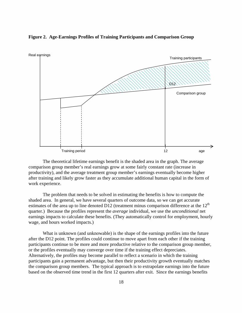
Cost-Benefit Analyses11

Earnings. Benefits and costs are projected for the “average” participant. Figure 2 shows the earnings profiles for the average individual in the treatment group and in the comparison group. The hypothesis used to construct these profiles is that encountering a workforce development program enhances an individual’s skills and productivity (thus increasing wage rates) and increases the likelihood of employment. Thus, after the training period, the treatment earnings profile is above the comparison earnings profile (both hourly wage and employment net impacts are positive.) During the training period, the treatment earnings will be below the comparison earnings, on average. These are the foregone costs of training in the form of wages that are given up by the participant while he or she is receiving training.

11 This discussion will present general methodological issues. Readers can find the specific parameters or

estimates that were used in the source reports.

- 6 - 5 - 4 - 3 - 2 - 1

registration

1999

200 200 2002

200 2004

exi+ + + + +5

+ +7

+ + +1 +1 +1

analysis period

18

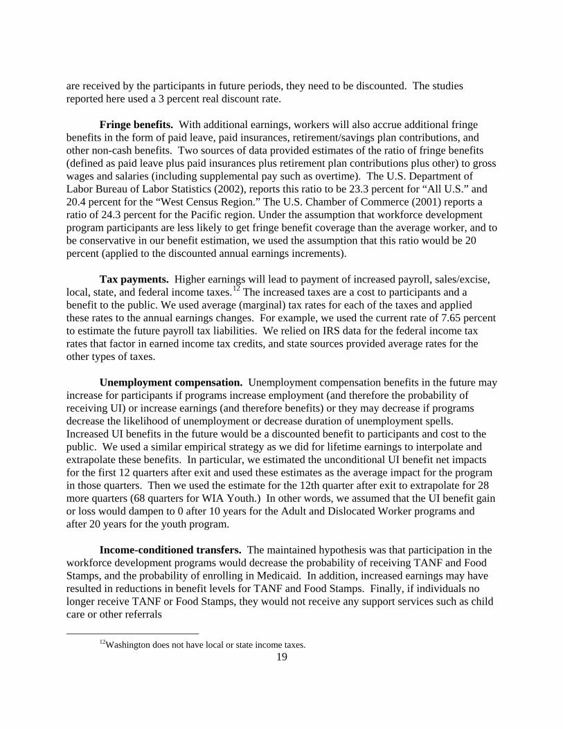
The theoretical lifetime earnings benefit is the shaded area in the graph. The average

comparison group member’s real earnings grow at some fairly constant rate (increase in productivity), and the average treatment group member’s earnings eventually become higher after training and likely grow faster as they accumulate additional human capital in the form of work experience.

The problem that needs to be solved in estimating the benefits is how to compute the

shaded area. In general, we have several quarters of outcome data, so we can get accurate estimates of the area up to line denoted D12 (treatment minus comparison difference at the 12th quarter.) Because the profiles represent the average individual, we use the unconditional net earnings impacts to calculate these benefits. (They automatically control for employment, hourly wage, and hours worked impacts.)

What is unknown (and unknowable) is the shape of the earnings profiles into the future

after the D12 point. The profiles could continue to move apart from each other if the training participants continue to be more and more productive relative to the comparison group member, or the profiles eventually may converge over time if the training effect depreciates. Alternatively, the profiles may become parallel to reflect a scenario in which the training participants gain a permanent advantage, but then their productivity growth eventually matches the comparison group members. The typical approach is to extrapolate earnings into the future based on the observed time trend in the first 12 quarters after exit. Since the earnings benefits

Real earnings

Training period

D

D12

12

Comparison group

Training participants

age

Figure 2. Age-Earnings Profiles of Training Participants and Comparison Group

19

are received by the participants in future periods, they need to be discounted. The studies reported here used a 3 percent real discount rate.

Fringe benefits. With additional earnings, workers will also accrue additional fringe

benefits in the form of paid leave, paid insurances, retirement/savings plan contributions, and other non-cash benefits. Two sources of data provided estimates of the ratio of fringe benefits (defined as paid leave plus paid insurances plus retirement plan contributions plus other) to gross wages and salaries (including supplemental pay such as overtime). The U.S. Department of Labor Bureau of Labor Statistics (2002), reports this ratio to be 23.3 percent for “All U.S.” and 20.4 percent for the “West Census Region.” The U.S. Chamber of Commerce (2001) reports a ratio of 24.3 percent for the Pacific region. Under the assumption that workforce development program participants are less likely to get fringe benefit coverage than the average worker, and to be conservative in our benefit estimation, we used the assumption that this ratio would be 20 percent (applied to the discounted annual earnings increments).

Tax payments. Higher earnings will lead to payment of increased payroll, sales/excise,

local, state, and federal income taxes.12

The increased taxes are a cost to participants and a benefit to the public. We used average (marginal) tax rates for each of the taxes and applied these rates to the annual earnings changes. For example, we used the current rate of 7.65 percent to estimate the future payroll tax liabilities. We relied on IRS data for the federal income tax rates that factor in earned income tax credits, and state sources provided average rates for the other types of taxes.

Unemployment compensation. Unemployment compensation benefits in the future may increase for participants if programs increase employment (and therefore the probability of receiving UI) or increase earnings (and therefore benefits) or they may decrease if programs decrease the likelihood of unemployment or decrease duration of unemployment spells. Increased UI benefits in the future would be a discounted benefit to participants and cost to the public. We used a similar empirical strategy as we did for lifetime earnings to interpolate and extrapolate these benefits. In particular, we estimated the unconditional UI benefit net impacts for the first 12 quarters after exit and used these estimates as the average impact for the program in those quarters. Then we used the estimate for the 12th quarter after exit to extrapolate for 28 more quarters (68 quarters for WIA Youth.) In other words, we assumed that the UI benefit gain or loss would dampen to 0 after 10 years for the Adult and Dislocated Worker programs and after 20 years for the youth program.

Income-conditioned transfers. The maintained hypothesis was that participation in the

workforce development programs would decrease the probability of receiving TANF and Food Stamps, and the probability of enrolling in Medicaid. In addition, increased earnings may have resulted in reductions in benefit levels for TANF and Food Stamps. Finally, if individuals no longer receive TANF or Food Stamps, they would not receive any support services such as child care or other referrals

12Washington does not have local or state income taxes.

20

For TANF/Food Stamps, we followed the same empirical strategy as we did for

unemployment compensation. We estimated net impacts for unconditional TANF benefits and Food Stamp benefits for the twelve quarters after program exit cohort and extrapolated beyond that period using the estimate from quarter +12. We again assumed that on average, the program participants may receive these benefits (or lose these benefits) for up to 40 quarters (or 80 quarters for the youth program) even though TANF is time limited to 20 quarters. The reason for going beyond 20 quarters is that these are averages for the entire program group, and the dynamics of recipiency will be assumed to continue for up to 10 years.

The typical pattern for the workforce development programs is that in the short term,

TANF benefits are decreased for participants who exit because, for the most part, employment rates increase—at least, some individuals leave the rolls. However, as time progresses, some workers begin to lose employment, or become single and have dependent children, and the group’s TANF net impact benefits become positive, although of relatively small magnitude.

We followed a similar empirical strategy for Food Stamps as we did for TANF. We

estimated net impacts for unconditional benefits for the twelve quarters after program exit and extrapolated beyond that period using the estimate from quarter +12. We again assumed that on average, the program participants may receive these benefits (or lose these benefits) for up to 40 quarters (or 80 quarters for the youth program).

The states did not make actual benefit/usage information for Medicaid available, so we

estimated net impacts of actually being enrolled in Medicaid. Our hypothesis was that training participants will tend to decrease their enrollment rates as they become better attached to the labor force over time and will thus lose eligibility. We converted Medicaid enrollment into financial terms by multiplying the average state share of Medicaid expenditures per quarter times the average number of household members per case. As with TANF and Food Stamps, this is a benefit to the participant and a cost to the public. To interpolate/extrapolate the net impact of a program on Medicaid eligibility, we either averaged or fit a linear equation time series of estimated enrollment net impacts.

Costs. Two types of costs were estimated for each of the programs. The first was

foregone earnings, which would be reduced earnings while the participants were actually engaged in the training programs. The second type of cost was the actual direct costs of the training.

Foregone earnings represent the difference between what workforce development

program participants would have earned if they had not participated in a program (which is unobservable) and what they earned while they did participate. The natural estimate for the former is the earnings of the matched comparison group members during the length of training. Specifically, we used (7) to estimate mechanistically the foregone earnings. Note that we did not discount foregone earnings, but did calculate them in real $.

21

(7) ( )1 1 0ˆ0.5

i i ii iForegone E E E d− − = × + − × ,

where, 1 0,E E− = avg. quarterly earnings (uncond.) for treatment group in quarter –1 and during training period, respectively.

1E = avg. quarterly earnings in 1st post-exit period for matched comparison group d = avg. training duration

i = indexes program

For the most part, the costs of providing services were supplied to us by the states. Staff members of the state agencies calculated these costs from administrative data on days in the program and daily cost information.

22

REFERENCES

Dehejia, Rajeev H., and Sadek Wahba. 1995. “Causal Effects in Non-Experimental Studies: Re-Evaluating the Evaluation of Training Programs. Working paper. Cambridge, MA: Harvard University.

Heinrich, Carolyn J., Peter R. Mueser, and Kenneth R. Troske. 2008. “Workforce Investment

Act Non-Experimental Net Impact Evaluation.” Report to U.S. Department of Labor. Columbia, MD: IMPAQ International.

Hollenbeck, Kevin. 2004. On the Use of Administrative Data for Workforce Development

Program Evaluation. Paper presented at the U.S. Department of Labor, Employment and Training Administration’s “2004 National Workforce Investment Research Colloquium” held in Arlington, VA, May 24.

———. 2009. Return on Investment Analyses of a Selected Set of Workforce System Programs

in Indiana. Kalamazoo, MI: W.E. Upjohn Institute for Employment Research. Hollenbeck, Kevin M., and Wei-Jang Huang. 2003. Net Impact and Benefit-Cost Estimates of

the Workforce Development System in Washington State. Technical Report No. TR03-018. Kalamazoo, MI: W.E. Upjohn Institute for Employment Research.

———. 2006. Net Impact and Benefit-Cost Estimates of the Workforce Development System in

Washington, State. Technical Report No. TR06-020. Kalamazoo, MI: W.E. Upjohn Institute for Employment Research.

———. 2008. Workforce Program Performance Indicators for The Commonwealth of Virginia.

Technical Report No. 08-024. Kalamazoo, MI: W.E. Upjohn Institute for Employment Research.

Imbens, Guido W. 2004. “Nonparametric Estimation of Average Treatment Effects Under

Exogeneity: A Review.” The Review of Economics and Statistics, 86(1): 4–29. Imbens, Guido W., and Joshua D. Angrist. 1994. “Identification and Estimation of Local

Average Treatment Effects.” Econometrica 62(2): 467–475. Mueser, Peter, Kenneth Troske, and Alexey Gorislavsky. 2007. “Using State Administrative

Data to Measure Program Performance.” Review of Economics and Statistics 89(4): 761–783.

U.S. Chamber of Commerce. 2001. The 2001 Employment Benefits Study. Washington, DC:

U.S. Chamber of Commerce.

23

U.S. General Accounting Office. 1996. Job Training Partnership Act: Long-Term Earnings and Employment Outcomes. Report HEHS-96-40. Washington, DC: U.S. Government Printing Office.

U. S. Department of Labor, Bureau of Labor Statistics. 2002. “Employer Costs for Employee

Compensation – March 2002.” News 02-346: entire issue.