worker profiling and reemployment services - ETA Advisories
431
WORKER PROFILING AND REEMPLOYMENT SERVICES EVALUATION OF STATE WORKER PROFILING MODELS FINAL REPORT MARCH 2007 Prepared for: U.S. Department of Labor Employment and Training Administration Office of Workforce Security Prepared by: Coffey Communications, LLC Bethesda, Maryland Authors: William F. Sullivan, Jr., Project Manager Lester Coffey Lisa Kolovich, Ph.D. (ABD) Charles W. McGlew Douglas Sanford, Ph.D. Richard Sullivan This project has been funded, either wholly or in part, with Federal funds from the Department of Labor, Employment and Training Administration under Contract Number AF-12985-000-03-30, Task Order 19. The contents of this publication do not necessarily reflect the views or policies of the Department of Labor, nor does mention of trade names, commercial products, or organizations imply endorsement of same by the U.S. Government.
Transcript of worker profiling and reemployment services - ETA Advisories
WORKER PROFILING AND REEMPLOYMENT SERVICES EVALUATION OF STATE WORKER PROFILING MODELS
FINAL REPORT
MARCH 2007
Prepared for:
U.S. Department of Labor Employment and Training Administration
Office of Workforce Security
Prepared by:
Coffey Communications, LLC Bethesda, Maryland
Authors:
William F. Sullivan, Jr., Project Manager
Lester Coffey Lisa Kolovich, Ph.D. (ABD)
Charles W. McGlew Douglas Sanford, Ph.D.
Richard Sullivan
This project has been funded, either wholly or in part, with Federal funds from the Department of Labor, Employment and Training Administration under Contract Number AF-12985-000-03-30, Task Order 19. The contents of this publication do not necessarily reflect the views or policies of the Department of Labor, nor does mention of trade names, commercial products, or organizations imply endorsement of same by the U.S. Government.

ACKNOWLEDGEMENTS
The contributors to this report were many. From the Office of Workforce Security, Ron Wilus
and Michael Miller provided overall direction and perspective that helped to bound and focus the
study. We are especially grateful to Scott Gibbons for his invaluable assistance and guidance
throughout the project. He was also most helpful in providing feedback on the various
approaches that were considered, helping to acquire needed data, and managing the OWS review
process. The reviewers included Wayne Gordon, Jonathan Simonetta, Stephen Wandner and
Diane Wood.
We are grateful to the State Workforce Agencies for their promptness in completing the surveys
and providing data needed to conduct the study. Without the information and data they
provided, the analyses and resulting product could not have been achieved.
Amy Coffey served as the managing editor and was assisted by Bernie Ankowiak and Carol
Johnson.

TABLE OF CONTENTS
EXECUTIVE SUMMARY .................................................................................................. 4
INTRODUCTION ............................................................................................................ 14
LITERATURE REVIEW .................................................................................................. 19
WPRS EVALUATION STUDY........................................................................................ 33
EXTENDED DATA ANALYSIS ...................................................................................... 41
CONCLUSION................................................................................................................ 83
REFERENCES ............................................................................................................... 85
APPENDICES................................................................................................................. 90
APPENDIX A – Survey Instrument................................................................... 91
APPENDIX B – Comparison Table of SWA WPRS Models ............................ 97
APPENDIX C – Reports for 53 SWAs and Decile Tables for 28 SWAs....... 111
APPENDIX D – Expanded Analyses for 9 SWAs .......................................... 271

Worker Profiling and Reemployment Services Evaluation of State Worker Profiling Models Final Report – March 2007
Coffey Communications, LLC Page 4
EXECUTIVE SUMMARY
The Worker Profiling and Reemployment Services (WPRS) system, mandated by Public Law
103-152 of the Unemployment Compensation Amendments of 1993, is designed to identify and
rank or score unemployment insurance (UI) claimants by their potential for exhausting their
benefits for referral to appropriate reemployment services. The goals of this report are to 1)
describe ways that state workforce agencies (SWAs) have implemented the worker profiling and
reemployment services system (WPRS), 2) describe the methodology used to evaluate SWA
worker profiling model accuracy, 3) determine the effectiveness of SWA models in profiling
unemployment insurance (UI) claimants most likely to exhaust their benefits, and 4) prepare a
summary of “best practices” (models) for SWAs to use in improving their WPRS systems.
With Department of Labor administrative support, we collected survey data for 53 SWAs (50
states, the District of Columbia, Puerto Rico and the Virgin Islands) regarding their WPRS
operations. The diversity of their operations is described in tabular form in Appendix B.
Individual reports for each SWA and territory are in Appendix C.
The survey responses demonstrated the variety of approaches SWAs use in the WPRS systems.
The following describes some highlights.
Summary of WPRS System Differences
• Seven SWAs use the Characteristic Screen Model.
• Forty-six SWAs use a Statistical Model. Of these, 38 use logistic regression (logit) as the functional form,
five use linear multiple regression, one uses neural network, one uses Tobit and one uses discriminant
analysis.
• One SWA does not use any variables. Instead, it provides an electronic file based on the characteristics of
all claimants who are eligible for WPRS services to the One-Stop Centers, and they determine the number
and type of claimants to be called in for service.
• Seventeen SWAs have never updated their models since they were put into use.
• The major reason for updates has been to convert the occupational classification system from DOT to SOC
or O*Net and industry classification system from SICs to NAICS.
• Twenty-nine SWAs have never revised their models since they were put into use.

Worker Profiling and Reemployment Services Evaluation of State Worker Profiling Models Final Report – March 2007
Coffey Communications, LLC Page 5
• Of those SWAs that have revised their models, five were completed and put into use in 2005.
• Forty-two SWAs run the model weekly. The remaining 11 run the model daily.
• Forty-nine SWAs run the model against the claimant first payment file. The remaining four run it against
the initial claim file.
• The list of eligible candidates is produced when the model is run for 47 SWAs and when a service provider
requests referrals for SWAs. In two SWAs, the list is produced weekly even though the model is run daily.
• Thirty SWAs use occupation as a variable in their model. Twelve SWAs use DOT codes as their
occupational classification system; 11 SWAs use the O*NET system (some directly and some based on
feedback from the One-Stop; the remaining SWAs use the SOC classification system).
• Thirty-nine SWAs use industry as a variable. The most common method to verify employment and
industry classification is a cross-match against the UI wage record files. Even if the industry classification
is not used in the model, it is collected for other purposes. Forty-eight SWAs use the cross-match method,
and the remaining five base the industry classification on the initial claim interview.
• Ineligibility for selection/referral to WPRS varies considerably. The most common reasons are:
o Obtain employment through a union hiring hall
o Interstate claimant
o Temporary layoff
o Will be recalled to previous employment
o First payment occurred five weeks or more from the date of filing the initial claim
Eligible candidates:
• In 50 SWAs, lists of candidates are either mailed or sent electronically to the reemployment services
provider. In most SWAs, the lists go directly to workshop/orientation staff, while in a few they go to local
management personnel. In three SWAs, the lists are sent to administrative staff for review before being
sent to the local service provider.
• The two most important determinants of the number of candidates to be served are staff availability and
space. Most of the decisions on the number to be served are made locally. However, in six SWAs the
number of claimants to be selected and referred is determined by central office personnel and/or a
negotiation between central and local office personnel.
• In all SWAs (with the exception of the one SWA that does not calculate a score) that use the statistical
model, candidates are sorted by their probability of exhaustion. In those SWAs that use characteristic
screens, all candidates who are eligible for WPRS services are listed.
Variables:
• Fifty SWAs use benefit exhaustion as the dependent variable in the WPRS model equation. Other
dependent variables used are:
o Specific benefit duration – one SWA
o Proportion of total benefits paid – one SWA
o Exhaustion of benefits and long-term unemployed

Worker Profiling and Reemployment Services Evaluation of State Worker Profiling Models Final Report – March 2007
Coffey Communications, LLC Page 6
Independent variables used in statistical models vary widely. The majority of SWAs still use the variables
recommended by ETA when WPRS became law. These are:
• Industry (39 SWAs)
• Occupation (30 SWAs)
• Education (39 SWAs)
• Job tenure (40 SWAs)
• Local unemployment rate (24 SWAs)
We note that the above variables are entered into the models directly. Other SWAs may collect these variables and
not use them in their models, or use these variables to create other variables that are in the models, such as industry
unemployment rate.
Regarding our analysis of SWA profiling models, we had sufficient data to fully analyze nine
SWA profiling models, which are included in Appendix D. For all SWAs, we attempted to
replicate the existing SWA profiling score, develop a measure for UI benefit exhaustion for each
individual, develop a control for endogeneity1 (if possible), demonstrate the original model’s
effectiveness using a decile table and a comparison metric, develop an “updated” model and
demonstrate its effectiveness, develop a “revised” model and demonstrate its effectiveness,
develop a Tobit model and demonstrate its effectiveness, and analyze the effectiveness of
specific variables for discriminating between exhaustees and non-exhaustees for individuals with
the highest profiling scores, or Type I errors. Type I errors are individuals with high profiling
scores and therefore predicted to exhaust benefits but who actually do not exhaust them.
Our analysis includes two innovations that we think significantly improve the analysis of WPRS
models. First is the development of a metric that demonstrates the effectiveness of various
profiling scores. Second is the control for endogeneity. Because profiling and referral affect
1 Endogeneity refers to the problem that the profiling scores determine the individuals who get referred to reemployment services, and that these services may affect the probability of exhaustion. Therefore, observed exhaustion of profiled individuals would be a biased outcome measure. As described below, we developed a method for measuring and controlling for endogeneity.

Worker Profiling and Reemployment Services Evaluation of State Worker Profiling Models Final Report – March 2007
Coffey Communications, LLC Page 7
observed benefit exhaustion, it is necessary to control for the effect of reemployment services
when developing new profiling models.
Our metric is a statistic that demonstrates the effectiveness of a profiling score. Normally, the
metric ranges from 0 to 1. If a profiling score is as effective as a random number generator, then
the metric will be insignificantly different from 0. If a metric is a perfect predictor of UI benefit
exhaustion, then it will take a value of 1. A metric of 0.100, means that, for individuals with
high scores, the profiling score selects exhaustees 10 percent better than a random number. For
the metric, we also calculate a standard error. For SWAs, the standard error allows comparison
of multiple profiling models for statistically significant improvements. Details on how we
calculated the metric are included below.
Profiling data from SWAs were analyzed using the respective models of the SWAs. We used
those data submissions from SWAs which were complete and ran their models (without any
changes) to rank individuals by their profiling scores. This ranking was then used to select
individuals likely to exhaust benefits. For example, Arkansas had a calculated average
exhaustion rate of 49.9 percent or 26,273 claimants who exhausted their benefits. After ranking
individuals by profiling score, we selected the top 26,273 claimants with the highest profiling
scores. This ranked group would have an exhaustion percentage that was either better or worse
than the actual exhaustion rate experienced by Arkansas. We then revised the SWA’s model,
including changing some variables, and ran it to compare results.
Using data for Arkansas to gauge the predictive improvement of the SWA’s profiling over its
average exhaustion rate, we developed a metric that subtracts from 1.0 the ratio of the probability
of claimants not expected to exhaust over the share (% divided by 100) of claimants not

Worker Profiling and Reemployment Services Evaluation of State Worker Profiling Models Final Report – March 2007
Coffey Communications, LLC Page 8
exhausting benefits. The metric will be referred to as the profiling score effectiveness metric,
because it shows the extent that the SWA’s profiling model beat its average exhaustion rate.
Algebraically, the metric improvement for the data that Arkansas submitted is as follows:
Metric = 1 – (100 – Pr[Exh]) / {100 – Exhaustion}
= 1 – [Pr{non-exhaustion} / (Percent not exhausted)] = 1 – (100 – 54.64) / (100 – 49.9) = 1 – (45.36 / 50.1) = 1 – 0.905 = 0.095 = 9.5%.
The 9.5 percent is the percentage of additional exhaustees selected by the profiling score over a
score that is a random number. This percentage is the metric score.
We revised the profiling model for Arkansas. This new score was better than the original score.
For the top 49.9 percent of this new profiling score, or 26,273 claimants, the exhaustion rate was
57.62 percent; in the above formula, this number would be the new Pr[Exh]. For this revised
score, the metric was 15.4 percent. The 15.4 percent is the percentage of additional exhaustees
selected by the profiling score over a score that is a random number.
In all cases where the metric could be computed for a state, the SWA’s profiling model predicted
exhaustion in excess of the state average. Were the two values equal, the profiling model would
not be better, on average, than the random selection of individuals for likely exhaustion.
Arkansas’ profiling model predicted that 54.62 percent of the claimants would exhaust, more
than the 49.9 percent experienced by the state that included claimants with some low profiling
scores.

Worker Profiling and Reemployment Services Evaluation of State Worker Profiling Models Final Report – March 2007
Coffey Communications, LLC Page 9
If the profiling score were perfect, then the exhaustion rate of those selected would be 100
percent. If the profiling score were a random number, or not at all related to exhaustion, then we
would expect the exhaustion rate of those selected to be the same as for the sample as a whole, or
49.9 percent.
To summarize, for Arkansas, the exhaustion rate for the top 49.9 percent of the sample (26,273
individuals) was 54.64 percent, which suggests that the profiling score is better than a random
selection (54.64 percent is greater than 49.9 percent). Hence, the model beats the average by
about 4.7 percentage points. Our revised metric score beats the average by about 7.7 percentage
points. This information is displayed in Figure 1 below.
Figure 1
Illustration of Profiling Score Effectiveness Metric
Profiling score,In percentile
Exha
ustio
n ra
te
50.1%Top 49.9% of profiling score
49.9%
Box of interest
Arkansas’ original scorePr[exhaust] = 54.64%
Arkansas’ revised scorePr[exhaust] = 57.62%
0%
100%
0% 100%

Worker Profiling and Reemployment Services Evaluation of State Worker Profiling Models Final Report – March 2007
Coffey Communications, LLC Page 10
The metric ranges from 0.0, for a score that is no better than a random number, to 1.0 for a score
that predicts exhaustion perfectly. Graphically, the metric is illustrated by the figure above.
The figure is a rough illustration that contrasts the profiling score on the X axis, with individuals
ranked from lowest to highest score. On the Y axis is the exhaustion rate of individuals. With
higher profiling scores, we expect the exhaustion rate to increase.
The Box of Interest is the upper right rectangle defined by individuals with percentile profiling
scores above (1.0 minus the state exhaustion rate) and an exhaustion rate above 49.9 percent.
This area represents the set of non-exhaustees expected for a random profiling score.
If the profiling score were a random number, then the metric would be 0. The 49.9 percent of the
sample with the highest profiling score, or 26,273 individuals, would have an exhaustion rate of
49.9 percent. This rate is the same as the state overall. For the sample with the highest profiling
score, 26,273 individuals, 49.9 percent of them would exhaust, or 13,110 individuals. Non-
exhaustees would be 50.1 percent of the 26,273, or 13,163 individuals. This group of 13,163
individuals represents the box of interest. The extent that a profiling score selects these 13,163
as exhaustees determines the value of the metric. For a score that selects all 13,163 as
exhaustees, the metric will have a value of 1.0.
For Arkansas, the original score has a value of 54.64 percent, which is better than the state
exhaustion rate of 49.9 percent. The area under this line, as a percentage of the area of the entire
Box of Interest, is 9.5 percent. This area is shown in Figure 1 in black.
The revised score has a metric of 0.154, which implies that the area under this line, shown in the
Figure above the line for the original score is 15.4 percent of the area in the entire Box of

Worker Profiling and Reemployment Services Evaluation of State Worker Profiling Models Final Report – March 2007
Coffey Communications, LLC Page 11
Interest. The area corresponding to this revised score is shown in the figure as the sum of the
black and gray areas.
From our experience working with these profiling models, we recommend the following:
• Use a logistic regression model
• Include at least the following independent variables:
o Maximum benefit amount
o Wage replacement rate
o Education level
o Delay in filing for UI benefits
o Benefit exhaustion rate for the applicant’s industry
o Unemployment rate
o County/metro area of residence
o Industry and occupation codes
• Include continuous variables
• Include second-order variables
• Include interaction variables for models with more than one continuous variable
We note that exhaustion of UI benefits is the result of a very complex process that involves the
interaction of individual characteristics and environmental characteristics. None of the models
included enough information to explain a large percentage of exhaustion. However, our
development of a metric allows SWAs to compare the effectiveness of different versions of their
models.
The following table contains our metrics for assessing the effectiveness of profiling model scores
in 28 SWAs. Each row of the table contains the SWA name, a description of the type of
profiling score used, an indicator of whether the score has been corrected for endogeneity, the
exhaustion rate for the sample of individuals provided by the SWA, the number of individuals
with the highest profiling score (if the score were a perfect measure for exhaustion, then only

Worker Profiling and Reemployment Services Evaluation of State Worker Profiling Models Final Report – March 2007
Coffey Communications, LLC Page 12
these number of individuals would exhaust benefits), the rate of UI benefit exhaustion for the
individuals with high profiling scores, the metric, the variance of the metric, and the standard
error of the metric. For nine SWAs, Arkansas, District of Columbia, Georgia, Hawaii, Idaho,
New Jersey, Pennsylvania, Texas and West Virginia, we were provided all data to replicate the
original profiling score and were able to calculate an improved profiling score using the data
provided. We include these other scores on our table for comparison purposes.
Metric for Assessing the Effectiveness of SWA Profiling Scores SWA Profiling
score Control for
endogeneity? Exhaustion rate for the
state
Number of individuals
with the highest profiling score
Exhaustion rate for
individuals with high profiling scores
Metric Variance of the Metric
Standard Error of
the metric
Arizona original score Y 37.9 21,502 42.8 0.079 1.153 0.007
Arkansas original score N 49.9 26,273 54.6 0.095 1.804 0.008
Arkansas revised score N 49.9 26,273 57.6 0.154 1.686 0.008
Delaware estimated score* N** 39.0 4,207 42.4 0.055 1.227 0.017
District of Columbia
original score N** 56.0 5,385 60.3 0.097 2.277 0.021
District of Columbia
revised score N** 56.0 5,385 63.8 0.176 2.057 0.020
Georgia original score Y 35.7 75,994 44.0 0.129 1.017 0.004
Georgia revised score Y 35.7 75,994 47.3 0.181 0.976 0.004
Hawaii original score Y 39.7 3,526 43.9 0.069 1.248 0.019
Hawaii revised score Y 39.7 3,526 44.8 0.085 1.232 0.019
Idaho estimated score* Y 45.9 15,605 56.1 0.189 1.400 0.009
Idaho revised score Y 45.9 15,605 59.3 0.247 1.306 0.009
Iowa original score Y 15.4 2,456 16.2 0.010 0.368 0.012
Louisiana original score Y 42.6 22,825 51.9 0.161 1.282 0.007

Worker Profiling and Reemployment Services Evaluation of State Worker Profiling Models Final Report – March 2007
Coffey Communications, LLC Page 13
Maine original score Y 37.3 7,346 42.6 0.084 1.121 0.012
Maryland original score N** 50.4 18,974 54.1 0.075 1.877 0.010
Michigan original score Y 52.7 60,128 55.2 0.052 2.110 0.006
Minnesota original score Y 33.6 37,395 43.5 0.150 0.922 0.005
Mississippi original score N 45.5 8,208 47.3 0.033 1.620 0.014
Missouri original score Y 50.6 18,727 58.3 0.156 1.726 0.010
Montana original score Y 53.4 1,678 58.0 0.100 2.051 0.035
Nebraska original score N*** 95.2 44,098 95.5 0.054 36.698 0.029
New Jersey original score Y 62.4 67,030 66.0 0.096 2.947 0.007
New Jersey revised score Y 62.4 67,030 67.6 0.137 2.789 0.006
New York original score Y 40.4 205,729 55.5 0.253 1.073 0.002
Pennsylvania original score Y 46.1 103,172 51.2 0.095 1.564 0.004
Pennsylvania revised score Y 46.1 103,172 52.5 0.118 1.527 0.004
South Dakota original score N** 18.5 1,107 25.6 0.087 0.475 0.021
Tennessee original score Y 49.7 26,299 53.5 0.075 1.830 0.008
Texas original score Y 48.0 190,270 56.6 0.165 1.555 0.003
Texas revised score Y 48.0 190,270 56.9 0.170 1.545 0.003
Vermont original score N** 28.3 359 37.9 0.133 0.756 0.046
Virginia original score Y 23.3 21,186 27.7 0.057 0.611 0.005
West Virginia original score Y 41.0 12,209 50.7 0.164 1.205 0.010
West Virginia updated score Y 41.0 12,209 55.4 0.243 1.109 0.010
Wisconsin original score N 44.2 8,991 46.2 0.036 1.533 0.013
Wyoming original score N** 43.9 47 46.8 0.051 1.497 0.178
* SWA used a characteristic screen. We calculated a profiling score that used the same variables as the screen. ** SWA provided data indicating individuals who were referred, but the effect was insignificant. *** Nebraska had possible data problems, with 95% of the sample having more benefits paid than mba(maximum benefit allowance)

Worker Profiling and Reemployment Services Evaluation of State Worker Profiling Models Final Report – March 2007
Coffey Communications, LLC Page 14
INTRODUCTION
In 1993, Congress passed Public Law (P.L.) 103-152, an amendment to Section 303 of the Social
Security Act, which required state employment security agencies to establish and utilize a system
for profiling new Unemployment Insurance (UI) claimants. This legislation charged states with
developing a profiling system that:
• “identifies which claimants will be likely to exhaust regular compensation and will need
job search assistance services to make a successful transition to new employment;”
• “refers claimants identified pursuant to subparagraph (A) [first paragraph above] to
reemployment services, such as job search assistance services, available under State or
Federal law;”
• “collects follow-up information relating to the services received by such claimants and
the employment outcomes for such claimants subsequent to receiving such services and
utilizing such information in making identifications pursuant to subparagraph (A) [first
paragraph above];” and
• “meets such other requirements as the Secretary of Labor determines appropriate.”
This legislation also provided that as “a condition of eligibility for regular compensation for any
week, any claimant who has been referred to reemployment services pursuant to the profiling
system…participate in such services or in similar services unless the State agency charged with
the administration of the State law determines – (A) such claimant has completed such services;
or (B) there is a justifiable cause for such claimant’s failure to participate in such services.”
In effect, P.L. 103-152, required state workforce agencies (SWAs) to develop a profiling system
which met the above criteria and to place additional conditions of eligibility on claimants who
had been referred to reemployment services pursuant to the implemented profiling system as a
condition for receiving administrative grants.
Guidance in Implementing Worker Profiling Models Department of Labor (“DOL”) Field Memorandum No. 35-94 was published as a guide to state
administrators on the implementation of a system of profiling Unemployment Insurance
claimants and the provision of reemployment services to those claimants. DOL states that the

Worker Profiling and Reemployment Services Evaluation of State Worker Profiling Models Final Report – March 2007
Coffey Communications, LLC Page 15
primary objective of the Worker Profiling and Reemployment Services (WPRS) system is to
efficiently identify and match dislocated UI claimants with needed services by coordinating and
balancing the flow of referrals with available reemployment services, with matching being done
at an early stage in the claimant’s unemployment period in order to foster a rapid return to
productive employment in a manner that is cost effective.
The basic components of profiling are outlined in the memorandum as: (1) Identification - the
proper identification of claimants most likely to exhaust using either a statistical model or a non-
statistical claimant characteristic screen; (2) Selection and Referral – the process of selecting
and referring those UI claimants identified as dislocated workers to appropriate reemployment
service providers by no later than the end of the fifth week from each identified claimant’s UI
initial claim date; (3) Reemployment Services – the provision of appropriate reemployment
services to referred claimants, accomplished most effectively through a coordination of effort
between the UI system and service providers; and (4) Feedback – the establishment of an
information system between the UI system and service providers that will provide information
on the services provided to referred claimants and/or the claimant’s failure to report or to
complete such services in order to make determination on continuing UI eligibility as well as for
evaluation of the effectiveness of profiling and reemployment service systems.
In an examination of dislocation factors, DOL found the worker and economic characteristics or
“data elements” discussed below to be significantly associated with long-term employment. The
memorandum recommends that states incorporate as many of these data elements as they can
into their WPRS systems. The recommended data elements or factors are:
• Recall Status – identifies claimants who are permanently separated from their jobs
versus those with a definite date(s) of recall to work or who expect to be called back to
work but do not have a definite recall date(s). Claimants with recall date(s) are
considered much less likely to exhaust their UI benefits during their present spell of
unemployment. The memo recommends that this data element be used as part of an
initial or “first level” screen in order to include only permanently separated claimants in
the WPRS system and exclude those claimants with job attachment.

Worker Profiling and Reemployment Services Evaluation of State Worker Profiling Models Final Report – March 2007
Coffey Communications, LLC Page 16
• Union Hiring Hall Agreement – suggests that union-sponsored job search resources are
available that obviate the need for reemployment services traditionally needed by other
workers. This data element is also recommended to be used as part of a “first level”
screen to exclude claimants who use union hiring halls because they do not need
assistance given through the referral to a reemployment service provider.
• Education (level) – is closely associated with dislocation and that generally claimants
with less education are more likely to exhaust benefits than claimants with higher levels
of education.
• Job Tenure – is the measure of the length of time that a worker was employed in a
specific job. Tenure on the previous job is positively related to reemployment difficulty
because it measures knowledge and skills that are specific to the worker's previous job.
DOL cites studies that show the longer a worker is attached to a specific job, the more
difficulty the person has in finding an equivalent job elsewhere.
• Previous Industry – affects a claimant’s search for employment. This is due to the fact
that claimants who worked in industries that are declining relative to other industries in a
state experience greater difficulty in obtaining new employment than claimants who
worked in industries that are experiencing growth. DOL notes that obtaining data
concerning a claimant's former industry would be done by most states at the initial claims
process and that these data would then be matched with labor market information
regarding growing and declining industries within the state or sub-state areas.
• Previous Occupation – workers who are in low demand occupations can expect to
experience greater dislocation and greater reemployment difficulty than workers who are
in high-demand occupations. Occupational data will enable states to more effectively
identify those UI claimants in need of reemployment services and recommend that
occupation could be collected at the time of initial claim filing or via work registration.
Occupation could then be matched with labor market information regarding expanding
and contracting occupations in the state in order to determine which occupations are
high-demand and low-demand.
• Total Unemployment Rate – in sub-state areas with high unemployment, this variable
suggests unemployed workers will have greater difficulty becoming reemployed than
those workers in areas with low unemployment, all other conditions being equal. DOL

Worker Profiling and Reemployment Services Evaluation of State Worker Profiling Models Final Report – March 2007
Coffey Communications, LLC Page 17
recommends that states which are able to utilize unemployment data for sub-state regions
or areas use this information to enhance the accuracy of their profiling model.
The field memorandum also recognizes that, in most states, data about individual claimant
characteristics must be collected during the initial claims process, while in other states this
information may be available through other sources. Data elements that are most likely to be
collected through the initial claims process include the claimant’s recall status, union hiring hall
agreements, education level, years of tenure on the pre-UI job, and the industry and occupation
codes for their pre-UI jobs.
Evaluation Objectives and Design This report provides the Department of Labor with an examination of the states’ models while
controlling for selection and referral using data provided by the states. To the extent that
reemployment services affected subsequent exhaustion, the observed exhaustion rate would be
an invalid dependent variable for evaluating state models. The primary objective of this study
was to improve state worker profiling models by 1) establishing an approach for evaluation of
the accuracy of worker profiling models, 2) applying this approach to current state models to
determine how effective they were at predicting UI benefit exhaustion, and 3) based on the
results, developing guidance on best practices in operating and maintaining worker profiling
models.
The specific goals of this report are to:
• Describe the worker profiling and reemployment services system states have
implemented.
• Describe the methodology used to evaluate state worker profiling model accuracy.
• Determine the effectiveness of state models in profiling UI claimants most likely to
exhaust their benefits.
• Prepare a summary of “best practices” (models) for states to use in improving their
WPRS systems.

Worker Profiling and Reemployment Services Evaluation of State Worker Profiling Models Final Report – March 2007
Coffey Communications, LLC Page 18
Research Methods for this Report The primary source of data for this report is a survey that was sent to state administrators in
January 2006 that requested information and data on the operational and structural aspects of
their worker profiling models. Appendix A contains the survey instrument. The operational
section of the survey included a description of the state WPRS system operations, such as: how
often the model is run, how much control the area offices have over the number who are referred
for reemployment services, how often the model is updated, and who maintains and monitors
model performance. Structural aspects describe how the model predicts the likelihood of
claimants exhausting their benefits; including the data elements used, and how they are
categorized or transformed, how the state defines exhaustion, the functional form of the model,
and the model coefficients. Some states determined that the most efficient and effective way to
provide the highly technical structural information requested was to simply attach technical
reports or computer print-outs containing the pertinent information.
Secondary sources for the report include scholarly, legislative, governmental and professional
reports on the WPRS system, as well as previous evaluations of the system (see bibliography and
literature review). It is important to note that even though P.L. 103-152 was enacted in 1993,
limited research has been conducted to determine how effective states are at targeting those most
likely to exhaust benefits.

Worker Profiling and Reemployment Services Evaluation of State Worker Profiling Models Final Report – March 2007
Coffey Communications, LLC Page 19
LITERATURE REVIEW I. WPRS: Program Initiation and Research Support Enacted on March 4, 1993, P.L. 103-6 required the Secretary of Labor to establish a worker
profiling system within the Unemployment Insurance (UI) program nationwide. State
participation in this new program was voluntary at first. However, P.L. 103-152, enacted on
November 24, 1993, required the States to profile all new claimants for regular UI benefits (U. S.
Department of Labor, Employment and Training Administration 1994). The new law required
States to operate a system that “(A) identifies which claimants will be likely to exhaust regular
compensation and will need job search assistance services to make a successful transition to new
employment; (B) refers claimants identified pursuant to subparagraph (A) to reemployment
services, such as job search assistance services, available under any State or Federal law; (C)
collects follow-up information relating to the services received by such claimants and the
employment outcomes for such claimants subsequent to receiving such services and utilizes such
information in making identifications pursuant to subparagraph (A); and (D) meets such other
requirements as the Secretary of Labor determines are appropriate” (P.L. 103-152, Sec. 4.
Worker Profiling). Participation in the reemployment services program was required of everyone
claiming state UI benefits unless the claimant had recently completed a similar program or had
‘justifiable cause’ for not doing so.
The combination of worker profiling and reemployment services had its foundation in
demonstration projects that took place in the 1980s. Using characteristic screens to identify
those most likely to exhaust, the New Jersey Unemployment Insurance Reemployment
Demonstration Project (NJUIRDP) enrolled 8,675 claimants. Workers were assigned to one of

Worker Profiling and Reemployment Services Evaluation of State Worker Profiling Models Final Report – March 2007
Coffey Communications, LLC Page 20
three treatment groups: 1) Job Search Assistance (JSA) only; 2) JSA plus training/relocation
assistance; 3) JSA plus a cash bonus for early reemployment. An evaluation of the project
showed that all three treatment groups had increased employment and earnings and reduced
collection of benefits (Corson and Haimson 1996). These results were persuasive to
policymakers: “Based in part on the design and the initial findings from the NJUIRDP, the
Unemployment Compensation Amendments of 1993 mandated that states identify workers likely
to exhaust UI and refer them to reemployment services” (Corson and Haimson 1996, p.55).
Other UI reemployment experiments used random assignment of claimants to treatment groups.
Meyer (1995) looked at bonus experiments in Illinois, New Jersey, Pennsylvania and
Washington State, and he looked at five job search experiments (Charleston, New Jersey,
Washington, Nevada and Wisconsin), including some where the state increased enforcement of
the job search. In the bonus states, the results were positive: “First, the bonus experiments show
that economic incentives do affect the speed with which people leave the unemployment
insurance rolls….This is shown by the declines in weeks of UI receipt found for all the bonus
treatments, several of which are statistically significant” (Meyer 1995, p.124). Structured job
search appeared effective as well: “The job search experiments test several alternative reforms
which appear promising. The five experiments try several different combinations of services to
improve job search and increase enforcement of work search rules. Nearly all these
combinations reduce UI receipt and (when available) increase earnings” (Meyer 1995, p.128).
The Department of Labor defined the new Worker Profiling and Reemployment Services
(WPRS) system as “an early intervention approach for providing dislocated workers with

Worker Profiling and Reemployment Services Evaluation of State Worker Profiling Models Final Report – March 2007
Coffey Communications, LLC Page 21
reemployment services to help speed their return to productive employment. It consists of two
components: a profiling mechanism and a set of reemployment services” (U. S. Department of
Labor, Employment and Training Administration 1994, p.3). The profiling mechanism had one
purpose: to determine which claimants are likely to collect all of the benefits to which they are
entitled. The scope of the new profiling system was extensive: “Profiling will select those UI
claimants who are likely to be dislocated workers out of the broad population of UI claimants
and refer them to re-employment services early in their unemployment spell. Over the next
several years, the result will be to select about two million dislocated workers from eight to nine
million UI initial claimants” (U. S. Department of Labor, Employment and Training
Administration 1994, p.3).
The Department of Labor requirements were clear: Each state had to establish a profiling system
that identifies new claimants who were unlikely to return to their previous occupation or industry
and refers those workers to reemployment services that could reduce the duration of their
unemployment (U. S. Department of Labor, Employment and Training Administration, 1994).
While the other components of WPRS posed challenges for the states (e.g., UI staff had to
negotiate with local employment services program managers to ensure the delivery of job search
services that claimants needed), the method for selecting claimants who were likely to exhaust
was of prime importance. Although many states had traditionally identified permanently
separated claimants and considered many to be dislocated workers, there was no established
system nationwide for targeting these individuals or prioritizing reemployment services.

Worker Profiling and Reemployment Services Evaluation of State Worker Profiling Models Final Report – March 2007
Coffey Communications, LLC Page 22
The model provided to states by the Department of Labor was designed to accomplish several
objectives. It had to be sensitive to state economic conditions and understandable to UI staff in
the states. Unemployment Insurance policymakers had to be able to set thresholds for referral of
claimants in need of services. The result had to be selection of a target group of likely
exhaustees that could actually be provided services under existing staffing constraints (Worden
1993). A two-step method was created. First, in order to avoid interfering with workers’
connections to existing employers, claimants with a recall date were excluded. Workers whose
job search focused solely on union hiring halls were excluded as well, since they were unlikely
to profit from the job search services being offered. Second, five variables (education,
occupation, industry, job tenure, and the state unemployment rate) were used to identify and rank
by probability of exhaustion the group to be referred for services. An evaluation of the model
indicated that it would effectively select a target population that needed services: “Historic data
indicate that the model would target a group of claimants equal to 30 percent of the total UI
population, while including 53 to 60 percent of all UI recipients with serious reemployment
difficulties” (Worden 1993, p.126).
Although the Department outlined two approaches to developing a profiling method (i.e.,
statistical models and characteristics screening), it recommended that states use the statistical
model approach because the model predicted a probability of benefit exhaustion for each
claimant. However, the Department cautioned states that chose to use the model that adoption of
the national model was only the first step: “This profiling model is not meant to be standardized
for all States or to be constant over time. Rather, it is subject to modification by individual
States to meet their particular needs. The coefficients used in this profiling model should

Worker Profiling and Reemployment Services Evaluation of State Worker Profiling Models Final Report – March 2007
Coffey Communications, LLC Page 23
optimally be re-estimated based on State (and possibly sub-state) historical data for each
variable, in order to derive State-specific coefficients for the model. Additional variables can be
added to the model, in order to pick up factors specific to the state. The definitions of the
variables can be altered, if necessary, to reflect particular circumstances that are unique to the
State (U. S. Department of Labor, Employment and Training Administration, 1994, p.11).
II. WPRS: The First Four Years
A comprehensive review and evaluation of the first few years of WPRS implementation found
that states were, for the most part, following the directions provided by the Department of Labor
(Hawkins, Kreutzer, Dickinson, Decker, and Corson 1996). Focusing on data from the five
states that were initially funded to develop a program, as well as a survey of state program
managers, the research team found all states excluded workers with recall dates and attachments
to union hiring halls. Each state was able to develop and implement a method for identifying the
target group of likely exhaustees, although some states required expertise provided by area
universities and others. Most states used statistical models and adopted the same approach as the
original Department of Labor model: “Four of the five states that used statistical models
specified a binary indicator of UI benefit exhaustion as the dependent variable. These four states
all estimated the models of benefit exhaustion using logit regression analysis, which was also
used by DOL to estimate the prototype” (Hawkins et al 1996, p.III-6).
The State of Kentucky took a different approach. Based on a model developed by the Center for
Economic and Business Research, Kentucky specified the dependent variable as the proportion
of benefits collected. “Researchers at the Center adopted this dependent variable because they

Worker Profiling and Reemployment Services Evaluation of State Worker Profiling Models Final Report – March 2007
Coffey Communications, LLC Page 24
felt it provided greater information than the simpler binary exhaustion indicator. After
experimenting with several estimation methods, the researchers at the Center decided to estimate
the model using Tobit regression methods because they felt it provided the most accurate
predictions” (Hawkins et al 1996, p.III-6).
Generally, in building their models, States used the explanatory variables recommended by the
Department of Labor. Again, Kentucky was an exception: “the (Kentucky) model contained a
large number of explanatory variables, including those related to a claimant’s previous wage, UI
benefit parameters, reservation wage, pensions, assistance receipt, prior UI receipt, industry
growth, occupation growth, job tenure, work experience, reason for separation, county
unemployment rate, and county employment growth” (Hawkins et al 1996, p.III-7 & III-8).
The models were considered to be effective: “The models clearly identified claimants who were
most likely to exhaust their benefits” (Hawkins et al 1996, p.III-10). However, looking to the
future, the research team expressed concern that states might soon begin re-estimating their
models using samples that included WPRS participants.
The 1997 Report to Congress on the effectiveness of WPRS supported the evaluation findings
contained in the interim report. The research team concluded that claimants likely to exhaust
were being identified and referred for services early in their benefit year. Claimants who did not
need services were being excluded. Most states were using statistical models to identify and
rank WPRS participants. These participants were receiving more services than claimants who
were not referred (Dickinson, Decker, and Kreutzer 1997). There was also preliminary evidence

Worker Profiling and Reemployment Services Evaluation of State Worker Profiling Models Final Report – March 2007
Coffey Communications, LLC Page 25
that WPRS participants had favorable outcomes: “Estimates based on the early implementation
states provide reasonably strong evidence that WPRS, as it was implemented in these states,
significantly reduced UI receipt: For two of the three states that appeared to have the most
accurate data (Kentucky and New Jersey), the WPRS reduced benefit receipt by slightly more
than half a week per claimant, which translates into a UI savings of about $100 per claimant”
(Dickinson et al 1997, p.IV-4). Nevertheless, the research team recommended that the
Department of Labor and the states monitor WPRS more closely to make certain that the
claimants most likely to exhaust are being selected and referred for reemployment services.
At a conference in 1999, the same research team presented several conclusions based on their
investigations of state profiling methods: 1) states that were using characteristics screens were
not accurately identifying those claimants most likely to exhaust because they did not
differentiate among those who passed the screens; 2) the states that were using national
coefficients provided by the Department of Labor were not as successful as those that had
developed state-specific models; and 3) states need to continually update their models to reflect
recent changes in the economy, e.g., growth or decline of occupations and industries (Dickinson,
Decker, and Kreutzer 2002).
III. WPRS: Following the Report to Congress
In 1998, the Department of Labor closely reviewed the specifications used in the profiling
models of thirteen states. The results (Kelso 1999) indicated that the states not only had to
develop alternative specifications, but also had to introduce new data elements and variables in
order to achieve the purpose of profiling, i.e., identify the individuals most likely to exhaust

Worker Profiling and Reemployment Services Evaluation of State Worker Profiling Models Final Report – March 2007
Coffey Communications, LLC Page 26
benefits. For the most part, however, states were using benefit exhaustion for the dependent
variable and focused on the amount each claimant was paid during the benefit year. This
approach follows the national model, which envisioned a binary outcome: “Thus, the dependent
variable in the DOL model was coded as ‘1’ for exhaustees and ‘0’ for non-exhaustees. The
output of the model is a predicted probability between zero and one that each claimant will
exhaust benefits. Both the national and Maryland2 versions of the DOL model used logistic
regression, the preferred statistical technique that accounts for the complexities introduced by a
binary dependent variable…. A binary dependent variable is a special constrained case which
usually cannot be modeled using simple ordinary least squares (OLS) regression analysis…”
(Kelso 1999, p. 20).
Some states modified the DOL model, which coded as exhaustees only those who had collected
100 percent of their benefits. These states have used a lesser standard to determine exhaustion
(e.g., the claimant collected 90 percent of entitlement), set a minimum amount of weeks to
prevent identifying claimants whose benefit entitlement consisted of only a few weeks, or simply
coded all workers receiving federal extended benefits as exhaustees.
Other states decided to explore alternatives to a binary dependent variable (e.g., the number of
weeks claimed). The ratio of benefits drawn to potential benefit entitlement was also tested,
using ordinary least squares (OLS) regression. However, this alternative was not considered by
the reviewer to be more effective: “Experimentation with this dependent variable concluded that
using it in a WPRS model incurred significantly more estimation difficulties and gained little
with respect to predictive capability. Ultimately, this method was abandoned in favor of logistic 2 The State of Maryland was the test site for the DOL profiling model.

Worker Profiling and Reemployment Services Evaluation of State Worker Profiling Models Final Report – March 2007
Coffey Communications, LLC Page 27
regression using a binary dependent variable.…In general, since logistic regression is more
straightforward and well-supported in economic literature, and since it focuses on the
characteristics of claimants who exhaust benefits, it is the preferred method for targeting
claimants for WPRS” (Kelso 1999, p. 21).
States were also exploring the use of a wide variety of independent variables. Some states were
using continuous variables (can take on a range of values) instead of categorical indicators (can
take on a binary or restricted set of values) for the variables that had been determined to be good
predictors, e.g., education and job tenure. Industry of the claimant’s last job was found to be a
valuable predictor and states were able to include industry change rates. The impact of the
claimant’s occupation on exhaustion rates was less clear. Lack of consistency in assigning
occupational codes to claimants and the use of different occupational coding schemes in
determining rates of growth or decline created problems. More work was needed: “Few states at
this point have been able to incorporate meaningful occupational effects into their WPRS
systems. Since occupation would seem to have a great deal of intuitive value in forecasting
long-term unemployment, the challenge for the future is in developing reliable methods for
coding claimants’ occupations and collecting data that accurately measure the relative labor-
market demand for them” (Kelso 1999, p. 26).
States experimented with several other data elements: weekly benefit amount; wage replacement
rate; base year wage; potential duration; the time delay in filing for UI benefits following a
separation; the ratio of high quarter wage to base year wage; number of base period employers;
and benefits drawn on a seasonal basis.

Worker Profiling and Reemployment Services Evaluation of State Worker Profiling Models Final Report – March 2007
Coffey Communications, LLC Page 28
The evaluation of the 13 state models concluded with a reminder that further evaluation,
redesign, and updating of state models is critical to achieving the objectives of WPRS and that
new challenges will emerge: “The estimation of profiling equations will need to evolve over
time to avoid the omitted variable bias that could be otherwise introduced by the impact of re-
employment services on exhaustion outcomes. This is likely to require controls for both the
receipt of reemployment services and for the types of services completed” (Kelso 1999, p.33).
During 1998, workforce development professionals from both state and federal government
reviewed the first four years of WPRS and made several recommendations to improve the
system. The first recommendation dealt with the use of models: “Within State resource
constraints, States should update and revise their profiling models regularly, as well as add new
variables and revise model specifications, as appropriate. DOL should provide technical
assistance to the States in model development and collect and disseminate best practices from the
States” (Wandner and Messenger, eds. 1999, p.16). More specifically, the WPRS Workgroup
encouraged states to update the weights assigned to different variables in their models,
investigate the potential value of research done by other states, change model specifications
every few years and include a variable related to the claimant’s main occupation. DOL was
encouraged to assist states in testing new variables and making changes in model specifications.
Olsen, Kelso, Decker, and Klepinger (2002) investigated the effectiveness of profiling models in
predicting exhaustion of benefits. Using data from the Florida Job Search Assistance
Demonstration of 1995-1996 and the New Jersey UI Reemployment Demonstration Project, they

Worker Profiling and Reemployment Services Evaluation of State Worker Profiling Models Final Report – March 2007
Coffey Communications, LLC Page 29
compared the effects of both the initial screen for “recall” and the predicted probability of
exhaustion for both treatment and control groups. The models did identify claimants who were
likely to exhaust and both steps were important. “However, the targeting power of the model is
modest….Exhaustion seems to be very difficult to predict accurately with available demographic
and labor market data” (Olsen et al 2002, p.53).
The authors also investigated whether the implementation of the WPRS program itself will
seriously contaminate new estimates of the profiling models. Concerned that states would use
data that include claimants who received WPRS services to predict the behavior of new
claimants, they used data from the Florida Job Search Assistance Demonstration to construct
“contaminated” and “uncontaminated” profiling models and investigate whether the models were
equally accurate in identifying likely exhaustees. They concluded that there is little difference in
the groups identified by each model, thereby suggesting that contamination from mandatory
services under WPRS is not a serious issue as states re-estimate their models: “This conclusion
is consistent with previous research that measures fairly modest effects of WPRS on UI receipt,
because the contaminating effect of WPRS on exhaustion should only be large if WPRS
generates large reductions in UI receipt” (Olsen et al 2002, p.52).

Worker Profiling and Reemployment Services Evaluation of State Worker Profiling Models Final Report – March 2007
Coffey Communications, LLC Page 30
IV. Recent Evaluations and Modeling Improvements
Black, Smith, Berger, and Noel (2003) set out to determine the effects of being profiled on
claimant behavior. Using data from Kentucky and an experimental design that randomly
assigned claimants with the same profiling score into treatment and control groups, the research
team found that the profiling program was very cost-effective: mean weeks of unemployment
benefits were reduced by 2.2 weeks, the amount collected was reduced by $143, and the mean
gain in earnings from employment was about $1,000. The impacts of WPRS were substantial:
“The WPRS impacts reported here also tend to be larger than those reported from experimental
evaluations of job search assistance programs for UI claimants summarized by Meyer (1995)”
(Black et al 2003, p.1320).
Analysis of these data led to two other major findings: 1) most of the impact is due to claimants’
voluntarily leaving the unemployment rolls soon after being profiled and referred to
reemployment services, and 2) there was no significant relationship between the estimated
impact of treatment and the profiling score. The findings reinforce the value of further research
on the effectiveness of profiling models: “the underlying assumption of the WPRS program is
that those with the longest expected UI spell duration would benefit the most from the
requirement that they participate in reemployment services in order to continue to receive their
UI benefits. It is also assumed that treating these claimants will result in the largest budgetary
savings for the state UI systems. Our results provide little justification for either assumption, as
we do not find a monotone relationship between the profiling score and the impact of treatment”
(Black et al 2003, p.1325).

Worker Profiling and Reemployment Services Evaluation of State Worker Profiling Models Final Report – March 2007
Coffey Communications, LLC Page 31
Black, Smith, Plesca, and Shannon (2003) investigated alternative profiling models using UI
administrative data from Kentucky for fiscal years 1989-1995 and offered several
recommendations to states that could both simplify their existing models and improve their
predictive power. Since these years included very different economic conditions, the research
team expressed confidence that other states could rely on both their methodology and their
conclusions. Analysis of different approaches to estimating profiling models led to “six
substantive guidelines for the specification of UI Profiling models,” including: 1) a preference
for ordinary least squares estimation of linear models; 2) selection of a continuous measure as
the dependent variable; 3) elimination of variables describing local employment conditions; 4)
introduction of several additional variables that will increase the predictive power of the model
without increasing its complexity; 5) omission of regional economic variables; and 6)
acknowledgment that the business cycle does affect the predictive power of the model (Black,
Smith, Plesca, and Shannon 2003, pp.35-36).
Eberts and O’Leary (2003) redesigned the profiling model that the state of Michigan used since
1995 to meet the federal requirement for a WPRS system. After considering the
recommendations contained in the study by Black, Smith, Plesca, and Shannon (2003) and
exploring an alternate specification that predicts the “fraction of benefits drawn during the
benefit year,” Eberts and O’Leary recommended that the model be re-estimated retaining
exhaustion of benefits as the dependent variable: “This model performed slightly better and it is
easier to interpret” (Eberts and O’Leary 2003, p. 16). However, Eberts and O’Leary
recommended to the Michigan UI policymakers that the claimants profiled using the new model
be divided into 20 percentile groups, following Kentucky’s approach, and that Michigan UI refer

Worker Profiling and Reemployment Services Evaluation of State Worker Profiling Models Final Report – March 2007
Coffey Communications, LLC Page 32
groups with the highest scores to reemployment services first. Recognizing that wage record
data are now available to Michigan UI staff, the state was also encouraged to update the model
periodically with new variables.
V. Conclusion
In April, 2003, Christopher J. O’Leary, Senior Economist at the W.E. Upjohn Institute for
Employment Research, summarized for the U.S. Congress the impact of the WPRS system that
resulted from the passage of P.L. 103-152 in 1993. He pointed out to Congress that WPRS was a
unique approach to actually allocating services to people in need and that independent
evaluations of WPRS had documented the ability of profiling models to identify those most
likely to exhaust. Noting that about 85 percent of the states now use statistical models, O’Leary
testified that states need to improve their ability to accurately identify likely exhaustees: “At the
heart of WPRS is a statistical model that predicts the probability that a UI beneficiary will
exhaust his or her benefits… In order to ensure that the predictions are as accurate as possible,
states must be diligent in updating their statistical models on a regular basis” (O’Leary 2003).
He also recognized the need for some states to rely on universities and other professional groups
to redesign and test changes to their models.
Subsequently, O’Leary summarized the impact that program evaluations have had on the UI
system: “Research has guided the development of at least three aspects of the UI system:
programs for dislocated workers, targeted job search assistance and institutions for the
coordination of services. These in turn have led to the establishment of the WPRS system, one-
stop career centers, and State Eligibility Review Programs as part of the work test that is
administered by UI and one-stop career center staff” (O’Leary 2006, p.31).

Worker Profiling and Reemployment Services Evaluation of State Worker Profiling Models Final Report – March 2007
Coffey Communications, LLC Page 33
WPRS MODEL EVALUATION STUDY
As noted earlier, even though WPRS became law in 1993 and was implemented by the states
shortly thereafter, research on the effectiveness of the model to accomplish its goals has been
limited. Twenty-nine state workforce agencies (SWAs) have never revised the model, and of
those, 17 have never updated it. Major changes have taken place in the way initial UI claims are
taken. In-person filing occurs in only a few states. Many SWAs have moved to allowing
individuals to file using the telephone, and more recently, states are taking initial claims by the
Internet. The delivery of reemployment services has been decentralized, with local Workforce
Investment Boards (WIBs) determining the individuals to target for services, and in many cases,
who should provide the services. These factors contributed to a decision by DOL to undertake a
thorough examination of the effectiveness of WPRS models used by the SWAs.
This study has two major components: data collection and evaluation of the data and
information collected.
• Qualitative information and data regarding WPRS activities were collected by survey
from agencies (generally UI) responsible for profiling UI claimants and referring them to
reemployment services. The survey asked SWAs to supply narrative responses and 12
months of data in order for the contractor to analyze the effectiveness of their profiling
models. The survey consisted of two sections:
o An operational section that included an outline of the logistics of the model,
including model monitoring, frequency of the runs, controls on the flow of
candidates, business practices, etc.
o A structural section to gain insight into the model composition, the process used
to capture and validate data, and other associated practices. The information

Worker Profiling and Reemployment Services Evaluation of State Worker Profiling Models Final Report – March 2007
Coffey Communications, LLC Page 34
provided by the SWAs was utilized to replicate the screening of characteristics
and claims data of individual claimants.
• Twelve months of profiling data was used to replicate the WPRS models used by the
SWAs. The data included:
o Administrative data records used for profiling a claimant such as the initial claim,
continued claims, claimant characteristics and monetary determination(s).
o Data for any other explanatory independent (right-hand side) variables included in
the prediction equation such as local unemployment rate.
o Predicted values of the dependent (left-hand side) variable of the exhaustion
equation associated with profiling a claimant.
Our research was guided by three questions. First, how do the WPRS models and processes
operate and how accurate are the models currently in use? Second, what strategies or tactics
could be used to improve existing models? Third, based on our analyses, findings, and
conclusions, what are some potential best practices and models that state policymakers should
consider for improving their current WPRS systems?
To begin answering these questions, the Worker Profiling and Reemployment Services survey in
Appendix A was submitted for SWAs to complete. As noted above, the survey was divided into
two sections: Operational and Structural. Operational elements cover the attributes that are
found in the operating environment such as who is responsible for operating the WPRS system,
when the model is run, how the model is updated (run with new data to generate new statistical
parameters), how claims and other data are used, etc. Structural elements included the type
(characteristic screen or statistical) of model, the functional form (eg. logit, probit, tobit, linear,
or characteristic screen), and variables used to predict exhaustion. Together, the two sections
were designed to gain insight into the following:
• How frequently a SWA’s model is updated

Worker Profiling and Reemployment Services Evaluation of State Worker Profiling Models Final Report – March 2007
Coffey Communications, LLC Page 35
• How often the SWA’s model has been revised
• Whether or not there were model revisions planned
• How the SWA goes about determining and implementing revisions
• How initial claims are filed and what characteristics are captured at that time
• How frequently the model is run
• When a list of candidates is produced
• What file the model is run against (first pay records, other)
• Who determines occupation codes
• Who determines industry codes
• Who is not eligible for referral to WPRS services
• How many candidates are referred to reemployment services on a periodic ongoing basis
such as weekly
• What type of WPRS model and functional form is used for profiling claimants
• What the model’s dependent and independent variables and associated coefficients
consist of
• How the SWA defines exhaustion of UI benefits
With support from the U.S. Department of Labor, we collected survey responses from the 50
SWAs and the District of Columbia, Puerto Rico, and Virgin Islands. We also received datasets
from Arizona, Arkansas, Connecticut, Delaware, the District of Columbia, Florida, Georgia,
Hawaii, Idaho, Iowa, Louisiana, Maine, Maryland, Michigan, Minnesota, Mississippi, Missouri,
Montana, Nebraska, New Jersey, New York, North Dakota, Pennsylvania, South Carolina, South
Dakota, Tennessee, Texas, Vermont, Virginia, West Virginia, Wisconsin, and Wyoming. These
datasets, combined with the surveys, allowed us to analyze the models used by the SWAs to
identify claimants that were likely to exhaust their UI benefits and who will likely be referred to
reemployment service providers.

Worker Profiling and Reemployment Services Evaluation of State Worker Profiling Models Final Report – March 2007
Coffey Communications, LLC Page 36
We would have liked to use the data provided to also study the difference in SWA model
effectiveness during pre- and post-recessionary time periods. However, after examining the
models and datasets, we determined that this comparison would be invalid. First, SWAs had
markedly different models and data collection procedures. So using just 2003 data and
comparing the models of SWAs that were pre-recession with models of SWAs that were post-
recession would be invalid. We would not be able to separate the differences due to model type
and data quality from differences in general economic conditions. Second, within SWAs, we
considered comparing 1999 data with 2003 data, but several SWAs had revised their models
between 1999 and 2003. Therefore, we could not separate differences in model performance due
to differences in the model and differences in general economic conditions. Third, comparison
of 1999 and 2003 data within states also was due to differences in data quality for the two
periods. We could not separate differences in model performance due to data quality from
differences due to general economic conditions. Fourth, we did not develop a way to measure
whether states were in pre- or post- recessionary economies in 1999 and in 2003. It is not likely
that state business cycles would aligh with national ones. Therefore, we concluded that these
problems were intractable, and decided not to conduct an analysis on the differences in model
effectiveness for pre- and post- recessionary economies.
What was found from the WPRS SWA Submitted Surveys and Data
Outlined in our spreadsheet matrix in Appendix B are the individual SWA responses to the
WPRS survey that were transmitted to the SWAs in UIPL No. 9-06 on January 6, 2006. The
SWAs include the District of Columbia, Puerto Rico and the Virgin Islands. Fifty-three SWAs
submitted responses to the survey. Highlights of the survey responses are described below:
Worker Profiling and Reemployment Services Evaluation of State Worker Profiling Models Final Report – March 2007
Coffey Communications, LLC Page 37
• Seven SWAs utilize a Characteristic Screening Model.
• Forty-six SWAs utilize a Statistical Model. Of these, 38 use logistic regression (logit) as
the functional form (one of these does not use the variables - rather they electronically
transmit a file based on characteristics), five use linear multiple regression, one uses
neural network, one uses Tobit and one uses discriminant analysis.
• Seventeen SWAs have never updated their models since they were put into use.
• The principal reason for updates has been to convert the occupational (from DOT to SOC
and/or O*Net) and industry (from SICs to NAICS) classification systems.
• Twenty-nine SWAs have never revised their models since they were put into use. Of
those SWAs who have revised their models, five were completed and put into use in
2005.
• A trend in initial claims filing has been to encourage workers to file using the Internet.
Forty SWAs reported that initial claims are filed online. In one SWA, 95 percent of the
initial claims are filed using this method. When claims are filed using this method,
individuals select their occupational code from a “drop down” menu.
• Forty SWAs take claims over the telephone. Nationwide, the highest volume of initial
claims are filed via the phone.
• Four SWAs continue to take 100 percent of their initial claims in-person.
• Forty-two SWAs run the model weekly. The remaining 11 run the model daily.
• Forty-nine SWAs run the model against the claimant first payment file. The remaining
four run it against the initial claim file.
• The list of eligible candidates is produced when the model is run for 47 SWAs; when a
service provider requests referrals for four SWAs; weekly for two SWAs (even though
the model is run daily).
• Twelve SWAs use DOT codes as their occupational classification system; 11 SWAs use
the O*NET system (some directly and some based on feedback from the one-stop); and
the remaining SWAs use the SOC classification system.
• The most common method of verifying employment is a cross-match against the UI wage
record files. Forty-eight SWAs use this method, and the remaining five base the industry
classification on the initial claim interview.

Worker Profiling and Reemployment Services Evaluation of State Worker Profiling Models Final Report – March 2007
Coffey Communications, LLC Page 38
• Ineligibility for selection and referral to WPRS varies considerably. The most common
reasons for claimants to be ineligible for referral to WPRS services are:
o Obtain employment through a union hiring hall
o Interstate claimants
o In temporary layoff status
o Will be recalled to previous employment
o Received first payments five or more weeks from the date of filing the intitial
claim
Eligible candidates:
• In 50 SWAs, lists of candidates are either mailed or sent electronically to the
reemployment services provider. In most SWAs, the lists go directly to
workshop/orientation staff, while in a few they go to local management personnel. In
three SWAs, the lists are sent to central office staff to review the list and send it to the
local service provider.
• The two most important determinants of the number of candidates to be served are
staff availability and space. Most of the decisions on the number to be served are
made locally. However, in six SWAs the number of claimants to be selected and
referred is determined by central office personnel directly or after consultation and
negotiation with local staff.
• In all SWAs that use a statistical model, candidates are ranked by their probability of
exhaustion with those most likely to exhaust having the highest scores. Maryland
was an exception, ranking in reverse order.
Seven SWAs (Delaware, Idaho, Massachusetts, New York, Ohio, Puerto Rico, and the Virgin
Islands) used characteristic screens to separate claimants into those who would be eligible for
referral to WPRS services and those who would not.
The majority of the SWAs used logistic regression to estimate the probability of exhaustion for
UI benefit recipients. These SWAs often used threshold scores that determine who is likely to
exhaust UI benefits. Individuals with predicted probability scores at or above a “cut off” point

Worker Profiling and Reemployment Services Evaluation of State Worker Profiling Models Final Report – March 2007
Coffey Communications, LLC Page 39
are identified as potential benefit exhaustees. These individuals are then pooled and ranked in
descending order by predicted probability score for referral to reemployment services.
Dependent variables used in profiling models:
• Fifty SWAs use benefit exhaustion as the dependent variable in the WPRS model
equation. Other dependent variables used are:
o Specific benefit duration – one SWA
o Proportion of total benefits paid – one SWA
o Exhaustion of benefits and long-term unemployed
Independent variables used in WPRS models to predict likely exhaustees vary widely. The
majority of SWAs still utilize the variables recommended by ETA when WPRS became law.
They are:
• Industry (39 SWAs)
• Occupation (30 SWAs)
• Education (39 SWAs)
• Job tenure (40 SWAs)
• Local unemployment rate (24 SWAs)
Additional variables beyond those used in the original prototype model:
• Wage replacement rate (15 SWAs)
• Time from employment separation to the date the claim is filed, known as delay in filing
(15 SWAs)
• Number of employers in the base period (8 SWAs)
• Potential duration (7 SWAs)
Evaluation of Characteristic Screen and Statistical Models
The characteristic screen approach to estimating the predicted probability of benefit exhaustion is
simple. Individuals are profiled based on their characteristics – such as industry of employment,

Worker Profiling and Reemployment Services Evaluation of State Worker Profiling Models Final Report – March 2007
Coffey Communications, LLC Page 40
county of residence, occupational title, and/or number of years tenure at their most recent
employer. Individuals who fit the model’s characteristics are considered likely to exhaust and
potentially referred to reemployment services. All other individuals are not referred. The
characteristic screen model only divides individuals into two classes – those who are likely to
exhaust and those who are not. In contrast, the statistical model usually calculates for each
individual a probability of exhaustion that can take many values.
From the SWA surveys and data, we found there were seven SWAs that used characteristic
screens. The characteristic screen has both strengths and weaknesses. It can be tailored to
various subsets of applicants and can be revised quickly as economic conditions change. That is,
individuals within an industry, such as manufacturing, are selected very differently from
individuals from the retail trade industry. However, characteristic screens may also leave out
many individuals who are likely to exhaust and/or select individuals who are not likely to
exhaust. For example, individuals from the mining industry might not be selected on the basis of
any variable except duration and county of residence, depending on the structure of the
characteristic screen. It is possible that SWAs will exclude individuals who are potential benefit
exhaustees due to one characteristic. The characteristic screens do not allow for multiple
characteristics to be considered simultaneously, and do not weight characteristics. The result of
the characteristic screen is binary, while the statistical models generate probabilities that allow
reemployment services to prioritize individuals according to their likelihood of exhausting
benefits.

Worker Profiling and Reemployment Services Evaluation of State Worker Profiling Models Final Report – March 2007
Coffey Communications, LLC Page 41
EXTENDED DATA ANALYSIS
We conducted an extended data analysis on the data from nine SWAs: Arkansas, the District of
Columbia, Georgia, Hawaii, Idaho, New Jersey, Pennsylvania, Texas, and West Virginia. We
attempted to conduct the extended analysis for each SWA, but data problems limited the number
to nine. We only conducted the extended analysis for SWAs where we could replicate the state
profiling score, which implied that we had all the variables and coefficients used in the model.
In addition, we needed data on the state exhaustion rate to analyze the profiling score
effectiveness. One SWA, Wyoming, gave us all the necessary data and we were able to replicate
the profiling score. However, Wyoming’s sample size was only 107, which was not sufficiently
large to conduct a reliable extended analysis. For each state, we describe the variables,
coefficients, or exhaustion rate problem in Appendix C.
For each SWA, we attempted to perform the following eight-step analysis.
1. Understand and replicate the profiling model
2. Test for endogeneity in the model
3. Demonstrate the effectiveness of the original profiling score, corrected for endogeneity
4. Update the model using current data
5. Revise the model by refining the variables and adding second order and interaction terms
6. Apply a TOBIT model
7. Use metrics to evaluate model effectiveness
8. Analyze the variables that appear to best reduce Type I errors or improve the
performance of the model for individuals with high profiling scores
A detailed presentation of our analyses for each SWA is in Appendix D. In the sections below,
we describe the statistical procedures used in each step. At the end of this section, we offer
conclusions regarding which SWAs have the best models in terms of predicting benefit

Worker Profiling and Reemployment Services Evaluation of State Worker Profiling Models Final Report – March 2007
Coffey Communications, LLC Page 42
exhaustion. For purposes of this section, the term “endogeneity” refers to situations in which the
independent variables used for predicting the probability of benefit exhaustion are also
influenced by the referral to reemployment services, and therefore, influenced the derivation of
the probability of benefit exhaustion.
Step 1 - Understand and Replicate the Profiling Model
Replication of the SWA-provided probability of exhaustion scores was paramount to our analysis
of the profiling models currently used by SWAs. By successfully replicating their profiling
scores, we were able to develop a baseline from which we could gauge improvements in our
model revisions. Using those profiling scores in conjunction with the model specifications and
provided datasets, we are able to provide each SWA with an overall analysis of how well its
current model performs, and we can provide ways in which their current model can be adjusted
to increase predictive performance.
While every effort was made to analyze all data submitted, we were unable to replicate the
predicted probability scores and/or profiling model for a number of datasets for a number of
SWAs. However, for those SWAs that provided profiling scores and data that allowed us to
replicate the profiling scores, we found results that should be useful and applicable to other
SWAs seeking to improve their profiling models.
We analyzed the data for each individual in the dataset. First, we categorized or transformed the
data as needed to replicate the structure used in the profiling model. For example, there could be
a variable for “delay in filing” measured in days, but the profiling model categorized this
continuous variable into five possible SWAs: 1) lag of 0 to 1 day, 2) lag of 2 to 5 days, 3) lag of

Worker Profiling and Reemployment Services Evaluation of State Worker Profiling Models Final Report – March 2007
Coffey Communications, LLC Page 43
6 to 10 days, 4) lag of 11 to 20 days, and 5) lag of 21 or more days. To replicate the model, all
of these possible categories would need to be computed from the SWA-supplied data.
Second, for each individual, we replicated the profiling score by multiplying the variables by the
SWA-supplied coefficients and doing any other needed transformations. One common
transformation was the logistic transformation. If the sum of the variables times the coefficients
were S, the logistic transformation would be eS/(eS+1). This transformation has the desirable
property of always taking a value between 0.0 and 1.
Third, we compared our computed probability of exhaustion with the SWA-supplied profiling
score. We analyzed any discrepancies in order to check for errors in our calculations or data
problems. This exercise helped us understand how a SWA calculated its profiling score.
The analysis of SWA datasets that used characteristic screens involved an extra step. For these
SWAs, we first estimated a proxy profiling score (continuous variable) that used the same
information as the characteristic screen. We conducted a logit analysis using exhaustion as the
dependent variable and the variables used by the SWA in its screen as independent variables.
Then we saved the model’s predicted probability as a proxy profiling score.
Step 2 - Test for Endogeneity in the Model
An essential part of our analysis was to determine how successful profiling models were at
classifying potential benefit exhaustees and at determining which variables are important in
explaining the differences between exhaustees and non-exhaustees. Based on datasets provided

Worker Profiling and Reemployment Services Evaluation of State Worker Profiling Models Final Report – March 2007
Coffey Communications, LLC Page 44
by the SWA, we found that the majority included a binary variable indicating whether or not
individuals had been referred to reemployment services.
Each SWA has its own process for determining the number of claimants to refer to services, how
they would be notified to report to a service provider, and what services they could receive. As
mentioned earlier, no data were collected on what reemployment services each SWA provided or
made available to referred individuals. For the purposes of our analysis, we were primarily
interested in determining whether or not the referral to reemployment services had an effect on
benefit exhaustion.
If referral to reemployment services did have an effect on benefit exhaustion, then we have a
problem of endogeneity that will require a correction. By endogeneity, we mean that the
independent variables used for predicting the probability of benefit exhaustion are also
influenced by the referral to reemployment services and affected benefit exhaustion.
The problem of endogeneity can be described using two points in time. At time 0, individuals
who apply for UI benefits are profiled. Their individual characteristics are used in a statistical
model to predict the probability that they will exhaust benefits. The model then generates a
score that is used by the UI system to refer individuals for reemployment services.
At time 1, or over the next year, some individuals will exhaust their UI benefits. Our task is to
assess the effectiveness of a SWA’s profiling model for predicting benefit exhaustion.
If we simply use the variables in the statistical model, or in aggregation as the profiling score, as
independent variables in a logistic regression model with observed exhaustion as a dependent

Worker Profiling and Reemployment Services Evaluation of State Worker Profiling Models Final Report – March 2007
Coffey Communications, LLC Page 45
variable, we have a possible endogeneity problem. Observed exhaustion is likely to be affected
by the services that individuals receive through the referral system. So there is a functional
relationship between the independent variables and observed exhaustion, which violates the
assumption of non-stochastic X3 in the statistical model.
For example, suppose the profiling score is a perfect predictor of the likelihood of exhaustion.
All individuals over a percentile score of 0.5 would exhaust UI benefits over their benefit year.
Also suppose that reemployment services are very effective, and that 75 percent of individuals
who receive these services get jobs before their UI benefits expire. Also, assume that individuals
with the top 20 percent of profiling scores receive reemployment services.
Given the above example, we will observe a profiling score with certain specific characteristics.
For individuals with percentile scores of 0.0 to 0.5, nobody will exhaust. For individuals with
percentile scores of 0.5 to 0.8, all will exhaust. But for individuals with percentile scores of 0.8
to 1, only 25 percent will exhaust because they were referred to reemployment services. When
we analyze the model, we will find that the model would not predict exhaustion very well, even
though in actuality it is perfect. Our other analyses would also be affected, because the variables
we use in our revised and updated models to predict exhaustion would not explain true
exhaustion; it would only explain the biased observed exhaustion.
Endogeneity will not be a problem if there is no effect of referral on subsequent exhaustion.
Thus, the test for endogeneity will first determine if there is an effect of referral to employment
services on exhaustion. And, second, the model will estimate a correction for endogeneity. 3 The non-stochastic X assumption refers to the assumption that the model is using independent variables (“X” variables) to explain variation in a dependent variable (“Y” variable). If the X variables have values that are in part determined by the dependent variable or by factors that also affect the dependent variable, then the assumption of independence between the X variables and the disturbance term will be violated. The model will not generate unbiased and valid estimates of the coefficients.

Worker Profiling and Reemployment Services Evaluation of State Worker Profiling Models Final Report – March 2007
Coffey Communications, LLC Page 46
In technical terms, the endogeneity problem can be described as follows. Endogeneity implies
that the cross product of e, the disturbance term, and B(hat)X, will not be zero. This violates a
fundamental assumption for unbiasedness for regression models of least squares, logit, logistic,
and TOBIT forms. The standard algorithm for estimating parameters breaks down. The solution
we propose is to first diagnose if there is an endogeneity problem.
To illustrate, the standard ordinary least squares regression equation takes the form:
Y = βX + ε
Y is the dependent variable, β is an array of coefficients, X is a matrix of independent variables
that begins with a column of “1”s, so that the first β is the coefficient for the constant term, and ε
is the disturbance term. Statistical analysis generates estimates for each β, called B(hat), and an
associated standard error, which is necessary to determine the parameter’s significance. In the
estimated model, there is an error term which is an estimate of ε, called e. So the result of the
analysis is a set of B(hat)s and associated standard errors.
Y = B(hat)X + e
In order to solve the original equation, statisticians normally make a number of assumptions,
including that on average, e = 0, and that the product of B(hat)X and e sums to zero across all
individuals. For the non-stochastic X problem, this assumption does not hold.
The solution we propose is to first diagnose if there is an endogeneity problem, or that referral
affects the probability of exhaustion, and then to make an adjustment to the model that corrects
for the “referral effect.”

Worker Profiling and Reemployment Services Evaluation of State Worker Profiling Models Final Report – March 2007
Coffey Communications, LLC Page 47
To diagnose the problem, we borrow from the literature on DIF, or differential item functioning,
which is used to assess whether test items generate different response patterns for different
groups of people (Camilli & Shepard, 1994). For example, it has been shown that certain SAT
(Scholastic Assessment Tests) questions are answered more correctly by young men than young
women, especially if the question refers to sports or outdoors concepts.
With respect to our problem, we test whether the response pattern of UI benefit exhaustion for
referred individuals differs from that of non-referred individuals. The variables used for this are
the probability of exhaustion (Pr[exh]), the profiling score (score), and a binary variable for
referral (refer). Consider Figure 2.
Figure 2
Item Characteristic Curve
Pr[exh]
Score (varies from low to high predicted probability of exhaustion)
0
1
Low High
Figure 2 shows the typical shape of the relationship between profiling score and Pr[exh]. Higher
scores correspond to higher Pr[exh], and lower scores to lower Pr[exh]. The “S” shape of the

Worker Profiling and Reemployment Services Evaluation of State Worker Profiling Models Final Report – March 2007
Coffey Communications, LLC Page 48
curve is typical for logistic relationships. If the curve for the referred and non-referred
individuals is similar, then we can say that referral has no effect on the probability of exhaustion.
However, if there is an effect, it can be of two types. Consider Figure 3.
Figure 3
Uniform, or Signed, DIF
Pr[exh]
Score (varies from low to high predicted probability of exhaustion)
0
1
Low HighNon-referred individuals
referred individuals
Figure 3 shows different line curves for the referred and non-referred individuals. In this case,
for any value of score, the referred individuals have lower Pr[exh] than the non-referred. In
other words, referring means that on the average there is a benefit to referral that helps
individuals prevent exhaustion. This type of bias is called uniform or signed bias. There is also
unsigned or non-uniform bias as shown in Figure 4.
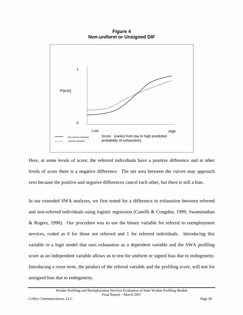
Worker Profiling and Reemployment Services Evaluation of State Worker Profiling Models Final Report – March 2007
Coffey Communications, LLC Page 49
Figure 4 Non-uniform or Unsigned DIF
Pr[exh]
Score (varies from low to high predicted probability of exhaustion)
0
1
Low HighNon-referred individuals
referred individuals
Here, at some levels of score, the referred individuals have a positive difference and at other
levels of score there is a negative difference. The net area between the curves may approach
zero because the positive and negative differences cancel each other, but there is still a bias.
In our extended SWA analyses, we first tested for a difference in exhaustion between referred
and non-referred individuals using logistic regression (Camilli & Congdon, 1999; Swaminathan
& Rogers, 1990). Our procedure was to use the binary variable for referral to reemployment
services, coded as 0 for those not referred and 1 for referred individuals. Introducing this
variable in a logit model that uses exhaustion as a dependent variable and the SWA profiling
score as an independent variable allows us to test for uniform or signed bias due to endogeneity.
Introducing a cross term, the product of the referral variable and the profiling score, will test for
unsigned bias due to endogeneity.

Worker Profiling and Reemployment Services Evaluation of State Worker Profiling Models Final Report – March 2007
Coffey Communications, LLC Page 50
The tests mirror the graphs shown above. According to the relevant literature, the tests are
conducted in the form of nested models. Introduction of each variable – the referral variable and
the cross term – requires estimation of a new logit model. We use a chi-squared test of (-2 times
the difference in model log likelihood) statistic to determine whether endogeneity is a significant
influence.
We then propose a remedy. It was to calculate and introduce a variable in the logistic regression
model that corrects for the referral effect. The new variable will have a fixed coefficient of 1,
and it is intended to bring the curve for referred individuals in line with the curve for non-
referred individuals. In the STATA statistical package, this variable is called an offset variable.
The exact calculation of the offset variable is described in the extended analyses. A typical
logistic regression that diagnoses endogeneity takes the following form:
Exhaustion = α + β1(profiling score) + β2(refer to services binary variable) + β3(cross term of
refer X score) + ε
Provided that β2 and β3 are significant, the correction for endogeneity is β2 X (refer to services
binary variable) + β3 X (cross term of refer X score). This variable will normally be a different
value for most individuals in the sample. The offset variable must be included in the model
without an estimated coefficient, or else the endogeneity problem will not be addressed. If a
software package that does not allow for offset variables, then a new algorithm should be
constructed using an appropriate statistical package.

Worker Profiling and Reemployment Services Evaluation of State Worker Profiling Models Final Report – March 2007
Coffey Communications, LLC Page 51
Step 3 - Demonstrate the Effectiveness of the Original Profiling Score Corrected for
Endogeneity
The next step was to recalculate the profiling score with a correction for endogeneity. The
example that follows shows our procedure. Some of the statistics presented will be described in
more detail later. The result of this procedure is a score that has correction for the bias due to
endogeneity and represents a more valid basis for determining the effectiveness of the profiling
model.
We will use data from Pennsylvania to illustrate the approach and to demonstrate how we correct
the original profiling score. First, we calculated the logistic regression model where only score
(along with a constant) is used to predict benefit exhaustion Pr[exh]. This example is slightly
complicated because there were two special classes of individuals, referred individuals and
exempt individuals. The analysis corrects for both signed and unsigned bias due to endogeneity
for both classes.
Logistic Regression Model with Score Only Logistic regression Number of
observations = 223906
LR chi2(1) = 1317.60 Prob > chi2 = 0.0000 Log likelihood = -153875.72 Pseudo R2 = 0.0043 exhaust Coefficient Std. Err. Z P>z
[95% Conf.
score 2.592343 .0717106 36.15 0.000 2.451793 2.732894 _cons -1.133801 .0274493 -41.31 0.000 -1.187601 -1.080001

Worker Profiling and Reemployment Services Evaluation of State Worker Profiling Models Final Report – March 2007
Coffey Communications, LLC Page 52
Next, we add the variables for referral and exempt to see if the addition of these variables
increases explanatory power. The test is a chi-squared test of the difference in the (-2 X log
likelihood) statistic for the nested models.
Logistic Regression Model with Score, Referral, and Exempt Logistic regression Number of
observations = 223906
LR chi2(3) = 3314.48 Prob > chi2 = 0.0000 Log likelihood = -152877.28
Pseudo R2 = 0.0107
exhaust Coefficient Standard
error z P>z [95% Conf. Interval]
score 2.835601 .0806119 35.18 0.000 2.677605 2.993598 referred individuals
.1078473 .0117285 9.20 0.000 .0848599 .1308348
exempt -.7580491 .0192067 -39.47 0.000 -.7956935 -.7204046 _cons -1.201052 .0296161 -40.55 0.000 -1.259098 -1.143005 The addition of the variables for referred and exempt individuals improves the log likelihood
from -153,875.72 to -152,877.28. This represents a significant difference, showing signed or
uniform bias from endogeneity. Now, we add two interaction terms (referral-not-exempt X
score, and exempt X score) to test for non-uniform or unsigned DIF.
Logistic Regression Model with Score, Referral-not-exempt, Exempt and Their Interactions Logistic regression Number of observations = 223906 LR chi2(5) = 3357.87 Prob > chi2 = 0.0000 Log likelihood = -152855.59 Pseudo R2 = 0.0109 exhaust Coefficient Standard
error z P>z [95% Conf. Interval]
score 3.126434 .0948357 32.97 0.000 2.940559 3.312308 referred individuals
.4218879 .0828933 5.09 0.000 .25942 .5843558

Worker Profiling and Reemployment Services Evaluation of State Worker Profiling Models Final Report – March 2007
Coffey Communications, LLC Page 53
exempt individuals
.0027421 .1330698 0.02 0.984 -.2580698 .263554
refer X score
-.784345 .2004544 -3.91 0.000 -1.177228 -.3914616
exempt X score
-1.857989 .3193107 -5.82 0.000 -2.483827 -1.232152
_cons -1.306397 .0347128 -37.63 0.000 -1.374433 -1.238361 Again, the addition of the interaction terms changed the log likelihood from -152,877.28 to -
152,855.59. This represents a significant difference, showing unsigned or non-uniform bias from
endogeneity. The coefficients suggest that the difference between the referred and non-referred
individuals is similar to that shown in Figure 4 above. For the referred and exempt individuals,
when score is 0 their logit is .4218879 X refer + .0027421 X exempt, which for both types of
individuals is a positive number. Therefore when score is 0, the referred and exempted
individuals will have estimated probabilities of exhaustion greater than other individuals. When
score is 1, referred individuals have logits of (.4218879-.784345) X refer, which is a negative
number below that of non-referred individuals. Similarly, for exempt individuals when score is
1, their logits are (.0027421-1.857989) X exempt, which is negative. So, similar to the pattern
shown in Figure 4, referred and exempt individuals (as the dotted line) will be above the curve
for low scores, and below the curve for high scores.
Our proposed remedy is to include a variable in the model with a fixed coefficient that controls
for the referral and exempt effect. This variable, called an offset variable, or offset, will account
for the deviation from the “score minus Pr[exhaust]” curve for individuals who are referred or
exempted. The value of this variable is derived from the coefficients of the above regression as:
.4218879*refnex+.0027421*exempt-.784345*xexrfnesco-1.857989*xexsco

Worker Profiling and Reemployment Services Evaluation of State Worker Profiling Models Final Report – March 2007
Coffey Communications, LLC Page 54
This value represents the difference between the Pr[exh] for referred and non-referred, and
exempt and non-exempt individuals. Adding this variable to the logistic regression as a fixed
coefficient variable should adjust referred and exempted individuals to the Pr[exh] that they
would have had if they were not referred or exempted.
By adjusting the original scores with this control for endogeneity, we can estimate the true
exhaustion rate for the original score. We calculate the model as follows. The logistic
regression has exhaustion as a dependent variable, with score as the independent variable and the
offset, named endogeneity control, to control for endogeneity. We saved the predicted values of
this model as a profiling score corrected for endogeneity.
Logistic regression Number of
observations = 223906
Wald chi2(1) = 1871.93 Log likelihood = -152855.59
Prob > chi2 = 0.0000
exhaust Coefficient Standard
error z P>z [95% Conf. Interval]
score 3.126434 .0722611 43.27 0.000 2.984804 3.268063 _cons -1.306397 .0276347 -47.27 0.000 -1.36056 -1.252234 endogeneity control
(offset)
To create tables that show the association between profiling score and subsequent benefit
exhaustion, we first ordered the resulting profiling scores in ascending order and then divided
them into deciles. We then looked at the mean exhaustion rate for each decile. Ideally, what we
would expect is for the lower deciles to have lower exhaustion rates and the higher deciles to
have higher exhaustion rates. This decile table is one way we can demonstrate the effectiveness
of each model.
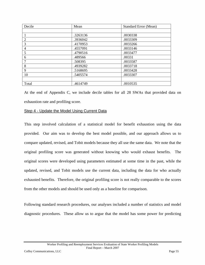
Worker Profiling and Reemployment Services Evaluation of State Worker Profiling Models Final Report – March 2007
Coffey Communications, LLC Page 55
Decile Mean Standard Error (Mean) 1 .3263136 .0030338 2 .3936042 .0033309 3 .4170953 .0033266 4 .4557091 .0033146 5 .4790516 .0033477 6 .489566 .00331 7 .508395 .0033587 8 .4939282 .0033718 9 .5168695 .0033428 10 .5405574 .0033307 Total .4614749 .0010535 At the end of Appendix C, we include decile tables for all 28 SWAs that provided data on
exhaustion rate and profiling score.
Step 4 - Update the Model Using Current Data
This step involved calculation of a statistical model for benefit exhaustion using the data
provided. Our aim was to develop the best model possible, and our approach allows us to
compare updated, revised, and Tobit models because they all use the same data. We note that the
original profiling score was generated without knowing who would exhaust benefits. The
original scores were developed using parameters estimated at some time in the past, while the
updated, revised, and Tobit models use the current data, including the data for who actually
exhausted benefits. Therefore, the original profiling score is not really comparable to the scores
from the other models and should be used only as a baseline for comparison.
Following standard research procedures, our analyses included a number of statistics and model
diagnostic procedures. These allow us to argue that the model has some power for predicting

Worker Profiling and Reemployment Services Evaluation of State Worker Profiling Models Final Report – March 2007
Coffey Communications, LLC Page 56
exhaustion and it conforms relatively well to the assumptions of a valid statistical analysis.
Using the example below4, we describe our procedures.
In our analysis of the SWA provided data, we used the statistical software package STATA to
perform our logistic regression analysis. In the made-up example that follows, we created a
dataset containing the following variables:
• Maximum Benefit Amount (MBA)
• Level of Education
• Wage Replacement Rate (WRR)
• NAICS Industry Code
For this example, much like with our analysis in Appendix D, we applied a logistical regression
to estimate the probability of UI benefit exhaustion. Using the data in our example, we used a
logistic regression to estimate the probability of UI benefit exhaustion:
Logistic regression Number of
observations = 52913
Wald chi2(26) = 713.03 Log likelihood = -36385.239 Prob > chi2 = 0.0000 Exhaust Coefficient Standard Error Z-Score P>z [95% Conf. Interval] MBA 0.00000986 0.00000828 1.19 0.235 -6.40e-06 .0000261 Education -.0427225 .0046309 -9.23 0.000 -.051799 -.0336461 WRR .7504832 .082631 9.08 0.000 .5885294 .912437 NAICS 0 -.3378624 .1024779 -3.30 0.001 -.5387155 -.1370093 NAICS 1 -.1215718 .1670119 -0.73 0.467 -.4489091 .2057655 NAICS 2 -.1938156 .0436113 -4.44 0.000 -.2792922 -.108339 NAICS 3 .1391356 .0343293 4.05 0.000 .0718515 .2064197 NAICS 4 -.0863585 .0329422 -2.62 0.009 -.1509241 -.0217929 NAICS 5 -.0528057 .0317214 -1.66 0.096 -.1149785 .0093671 NAICS 7 -.2384586 .0428455 -5.57 0.000 -.3224343 -.1544829 NAICS 8 .0991142 .0551996 1.80 0.073 -.0090751 .2073034 NAICS 9 .1364398 .0523579 2.61 0.009 .0338202 .2390593
4 We use a mix of data to illustrate our methods. Our objective is to provide simplicity of understanding and authenticity. Both contribute to a clear and useful illustration of our methods.

Worker Profiling and Reemployment Services Evaluation of State Worker Profiling Models Final Report – March 2007
Coffey Communications, LLC Page 57
Constant .2107467 .1084804 1.94 0.052 -.0018709 .4233643 These results show the variable coefficients, the standard errors of the variable coefficients, the
Z-score used to determine variable significance, the P-value for our Z-score, and the upper and
lower limits of the 95 percent confidence interval.
The variable coefficient from our regression represents the value to be applied to a variable
which, in our model, is used to predict the probability of benefit exhaustion. The value of this
coefficient falls between the lower limit and the upper limit of the confidence interval. For
example, for the maximum benefit amount we are 95 percent confident that its marginal impact
on benfit exhaustion, given the other variables in the regression, is between -0.0000064 and
0.0000261. This confidence interval is created by adding and subtracting approximately two
times the standard error of the coefficient.
From our results, we see that the Z-score for the MBA coefficient is 1.19, and it is calculated by
dividing the variable coefficient by its standard error as detailed below:
Z-score = Error Standard Variable
t Coefficien Variable
Z-score = ≈0.000008280.00000986
1.19 This Z-score is used to determine whether or not our coefficients are significantly different from
zero. This Z-score value is used to determine what the area under the standard normal curve is
that corresponds to this value. If our Z-score corresponds to an area of 95 percent or less we
cannot be confident that the true value for our coefficient is different than zero. For our analysis,
we are concerned only with P-values of 0.05 or smaller, which correspond to our being 95
percent confident that the true value of the coefficient is different from zero. Our Z-score of 1.19

Worker Profiling and Reemployment Services Evaluation of State Worker Profiling Models Final Report – March 2007
Coffey Communications, LLC Page 58
means that we are only about 76.5 percent sure that the variable is above 0. Therefore, we
conclude that MBA is not a significant factor in explaining exhaustion in our ficticious sample.
From the above STATA output we applied the corresponding coefficients to the corresponding
values for each variable. In doing so, we determined what the value of X based on the
coefficients and corresponding variables through the following equation:
X = MBA*(0.00000986) + Education*(-0.0427225) + WRR*(0.7504832)
+ NAICS 0*(-0.3378624) + NAICS 1*(-0.1215718) + NAICS 2*(-0.1938156)
+ NAICS 3*(0.1391356) + NAICS 4*(-0.0863585) + NAICS 5*(-0.0528057)
+ NAICS 7*(-0.2384586) + NAICS 8*(0.0991142) + NAICS 9*(0.1364398)
+ Constant
In the logistic transformation, the “X” calculated above will be implanted into the following
transformation:
eX/(eX+1)
e is a special number in statistics. It has a value of about 2.7.
The transformation yields a value between 0 and 1. The model will estimate all the parameters
such that the squared difference between the above transformed expression and the dependent
variable (ex., exhaustion - eX/(eX+1) is minimized.
We use classification tables to indicate how many benefit recipients were correctly classified as
likely to exhaust (defined as having a predicted probability score of 0.50 or higher). Sensitivity
is defined as the probability of a benefit recipient being properly classified as a benefit

Worker Profiling and Reemployment Services Evaluation of State Worker Profiling Models Final Report – March 2007
Coffey Communications, LLC Page 59
exhaustee. From the example set and profiling model we created, we found that from our sample
of 150,000 benefit recipients, 42,000 recipients were given profiling scores of 0.50 or higher and
exhausted benefits. Sensitivity here measures the probability that a benefit exhaustee is correctly
classified as an exhaustee. The equation used to determine sensitivity is defined as follows:
Pr( + D) = ExhausteesBenefit Number Total
ExhausteesBenefit IdentifiedCorrectly ofNumber
Pr( + D) = 6.070,00042,000
=
-------- True -------- Classified D ~D Total + 42000 10000 52000 - 28000 70000 98000 Total 70000 80000 150000 Classified + if predicted Pr(D) >= .50True D defined as exhaust != 0 Sensitivity Pr( + D) 60% Specificity Pr( -~D) 87.5% Positive predictive value Pr( D +) 80.76% Negative predictive value Pr(~D -) 71.43% False + rate for true ~D Pr( +~D) 12.5% False - rate for true D Pr( - D) 40% False + rate for classified + Pr(~D +) 19.23% False - rate for classified - Pr( D -) 28.57% Correctly classified 74.66% Specificity is defined as the probability of a benefit recipient being properly classified as a non-
benefit exhaustee. Here specificity is a metric that measures the probability that a non-exhaustee
is correctly classified as non-exhaustee. From our profiling model, 70,000 recipients were
identified as non-benefit exhaustees out of 80,000 benefit recipients that did not exhaust benefits.
The equation used to determine specificity is defined as follows:

Worker Profiling and Reemployment Services Evaluation of State Worker Profiling Models Final Report – March 2007
Coffey Communications, LLC Page 60
Pr( -~D) = ExhausteesBenefit -Non ofNumber Total
ExhausteesBenefit -Non IdentifiedCorrectly ofNumber
Pr( -~D) = 875.0000,80000,70
=
Positive predictive value (PPV) is a ratio of the number of correctly classified benefit exhaustees
to the total number of benefit recipients identified as benefit exhaustees. From our profiling
model, 42,000 recipients were correctly identified as benefit exhaustees out of 52,000 benefit
recipients that were identified as benefit exhaustees. The equation used to determine the positive
predictive value is defined as follows:
PPV = ExhausteesBenefit -Non as Identified RecipientsBenefit Total Exhaustees Benefit-Non True ofNumber
PPV = 8076.0000,52000,42
≈
Negative predictive value (NPV) is a ratio of the number of correctly classified non-exhaustees
to the total number of benefit recipients identified as non-exhaustees. From our profiling model,
70,000 recipients were correctly identified as non-exhaustees out of 98,000 benefit recipients that
were identified as non-benefit exhaustees. The equation used to determine the negative
predictive value is defined as follows:
NPV = ExhausteesBenefit -Non as Identified RecipientsBenefit Total Exhaustees Benefit-Non True ofNumber
NPV = 7143.0000,98000,70
≈
The additional metrics included in the classification table are measurements of false positives
and negatives. For examples, “False + rate for true ~D” measures how many benefit recipients
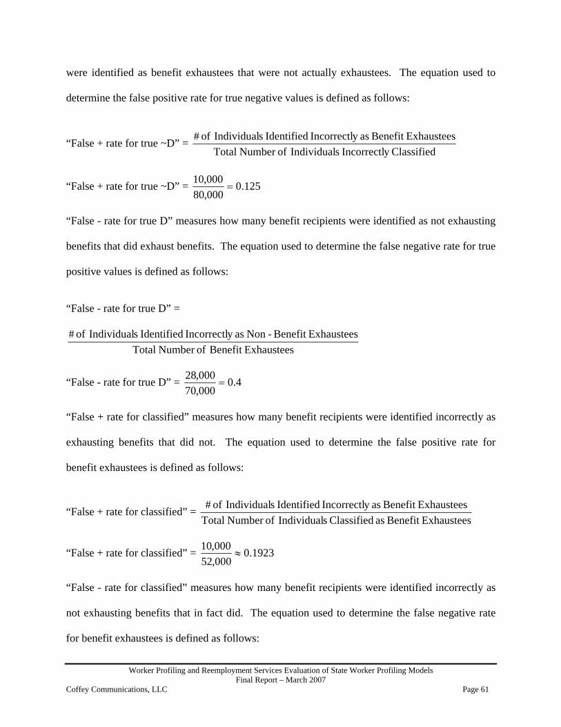
Worker Profiling and Reemployment Services Evaluation of State Worker Profiling Models Final Report – March 2007
Coffey Communications, LLC Page 61
were identified as benefit exhaustees that were not actually exhaustees. The equation used to
determine the false positive rate for true negative values is defined as follows:
“False + rate for true ~D” = Classifiedy Incorrectl sIndividual ofNumber Total
Exhaustees Benefit asy Incorrectl Identified sIndividual of #
“False + rate for true ~D” = 125.0000,80000,10
=
“False - rate for true D” measures how many benefit recipients were identified as not exhausting
benefits that did exhaust benefits. The equation used to determine the false negative rate for true
positive values is defined as follows:
“False - rate for true D” =
ExhausteesBenefit ofNumber TotalExhaustees Benefit-Non asy Incorrectl Identified sIndividual of #
“False - rate for true D” = 4.0000,70000,28
=
“False + rate for classified” measures how many benefit recipients were identified incorrectly as
exhausting benefits that did not. The equation used to determine the false positive rate for
benefit exhaustees is defined as follows:
“False + rate for classified” = ExhausteesBenefit asClassifiedsIndividualofNumber Total
Exhaustees Benefit asy Incorrectl Identified sIndividual of #
“False + rate for classified” = 1923.0000,52000,10
≈
“False - rate for classified” measures how many benefit recipients were identified incorrectly as
not exhausting benefits that in fact did. The equation used to determine the false negative rate
for benefit exhaustees is defined as follows:

Worker Profiling and Reemployment Services Evaluation of State Worker Profiling Models Final Report – March 2007
Coffey Communications, LLC Page 62
“False - rate for classified” = ExhausteesBenefit -NonasClassifiedsIndividualofNumber Total
Exhaustees Benefit-Non asy Incorrectl Identified sIndividual of #
“False - rate for classified” = 2857.0000,98000,28
≈
In addition to classification tables, we examined all logistic models for multicollinearity through
the examination of variance inflation factors and nonspherical disturbances through the analysis
of residuals and variable distributions. The models we include in this report all conform to
statistical assumptions.
From the above analysis, we see that in determining the effectiveness of a profiling model, we
must pay close attention to how the model classifies potential benefit exhaustees. In our example
above, we see that this particular model, using a profiling “cut off” score of 0.5, correctly
classifies approximately 75 percent of benefit exhaustees. Ideally, we would want to see high
values for sensitivity and specificity similar to the values in our analysis above.
With reference to our constructed dataset above, we estimate a new profiling score using the
updated model for an individual with a maximum benefit amount of $3,000, 12 years of
education, a wage replacement rate of 0.523871, and most recent employment in NAICS
industry 9, we apply the following variables values in the above equation:
Maximum Benefit Amount = 3,000 NAICS 0 = 0* NAICS 4 = 0*Education = 12 NAICS 1 = 0* NAICS 5 = 0*Wage Replacement Rate = 0.523871 NAICS 2 = 0* NAICS 7 = 0*Constant = 0.2107467 NAICS 3 = 0* NAICS 8 = 0* NAICS 9 = 1*
• Note: NAICS industry code variables are binary. In our example the claimant was last
employed in an industry corresponding to the one-digit NAICS code 9
X = (3,000)*(0.00000986) + (12)*(-0.0427225) + (0.523871)*(0.7504832)

Worker Profiling and Reemployment Services Evaluation of State Worker Profiling Models Final Report – March 2007
Coffey Communications, LLC Page 63
+ (0)*(-0.3378624) + (0)*(-0.1215718) + (0)*(-0.1938156) + (0)*(0.1391356) + (0)*(-0.0863585) + (0)*(-0.0528057) + (0)*(-0.2384586) + (0)*(0.0991142) + (1)*(0.1364398) + 0.2107467 X = 0.02958 – 0.51267 + 0.393156384 + 0 + 0 + 0 + 0 + 0 + 0 +0 + 0 + 0.1364398 + 0.2107467 X = 0.257252884
Next, we use this value, X, in the following logistic regression transformation to determine the
predicted probability of benefit exhaustion.
Pr[exh] = 1+X
X
ee
Pr[exh] = 140.25725288
40.25725288
+ee
Pr[exh] = 92.2933721591.29337215
Pr[exh] ≈0.56396
From the STATA provided coefficients, we find that our predicted probability of benefit
exhaustion for this individual is approximately 56 percent. It is important to note that by using a
logistic regression, the predicted probability of benefit exhaustion can range from only 0 percent
(very low probability of exhaustion) to 100 percent (very high probability of exhaustion). These
predicted probability of benefit exhaustion scores are used by some SWAs to determine who is
referred to reemployment services. For most SWAs, there is a “cut off” score that is used to
determine which eligible benefit recipients are referred to reemployment services.
After computing scores for all claimants, we can construct a decile gradient like the one below.
In this decile gradient, we see that for seven of our deciles the mean exhaustion rate hovers
around 0.25 or 25 percent. Ideally, we would expect to see a lower mean benefit exhaustion rate

Worker Profiling and Reemployment Services Evaluation of State Worker Profiling Models Final Report – March 2007
Coffey Communications, LLC Page 64
for the first decile and increasingly higher exhaustion rates for each decile there after. In
updating and revising the current profiling models used by SWAs, we hope to steepen the decile
gradient range, starting with lower exhaustion rates and having consistently higher exhaustion
rates for each decile. By improving the decile gradient range we are proving the proper
classification of benefit exhaustees.
Decile Mean Standard Error (Mean) 1 .25 .0047 2 .27 .0045 3 .26 .0046 4 .26 .0045 5 .23 .0045 6 .25 .0046 7 .26 .0047 8 .31 .0045 9 .34 .0047 10 .36 .0049 Total .28 .0046
Step 5 - Revise the Model by Refining the Variables and Adding Second Order and
Interaction Terms
The revised model is the same as the updated model except that variables are added to account
for nonlinear and second order interaction effects. For nonlinear effects, we generally make
more variables for all continuous variables. We calculate second order variables by subtracting
the mean value and squaring the variable. This allows us to limit the potential for
multicollinearity common with second-order terms. We also include variables for interaction
terms. To calculate these, we first subtracted the mean value from each variable and then
multiplied them.

Worker Profiling and Reemployment Services Evaluation of State Worker Profiling Models Final Report – March 2007
Coffey Communications, LLC Page 65
We included all continuous variables and all interaction terms if possible. We did conduct some
diagnostics of the variable sets where possible. If a variable had characteristics such as only
taking a few values, or was skewed, or was otherwise not suitable for use in the model, we
discarded it. In addition, we conducted tests for multicollinearity and removed variables that
significantly contributed to this problem. Details of our methods are included in the expanded
analyses in Appendix D.
To illustrate our approach to revised models, we include the model for Pennsylvania. The
updated model included continuous variables for a) 10-year historical exhaustion rate of primary
base year employer’s industry, and b) 12-month moving average for the labor market area. The
model below includes these variables, named “indexh” and “tur.” In addition, there are second
order variables for each named “xi2” and “xt2,” and an interaction term “xit.” Included below
are the classification table and decile table for this analysis.
Logistic regression Number of
observations = 223906
Wald chi2(15) = 4102.60 Log likelihood = -151684.36
Prob > chi2 = 0.0000
exhaust Coefficient Standard
error z P>z [95% Conf. Interval]
tenind -.1868556 .0088761 -21.05 0.000 -.2042524 -.1694588 eduind1 -.0968022 .0135224 -7.16 0.000 -.1233056 -.0702987 eduind2 .0675245 .0125174 5.39 0.000 .0429909 .0920581 decind -.0815156 .0383682 -2.12 0.034 -.156716 -.0063152 lowrr -.0599267 .0163153 -3.67 0.000 -.0919041 -.0279493 hibrr -.0258075 .078488 -0.33 0.742 -.1796411 .1280261 indexh 5.015172 .1268003 39.55 0.000 4.766648 5.263696 tur -.0423947 .0069549 -6.10 0.000 -.0560259 -.0287634 xit -.2096412 .0774124 -2.71 0.007 -.3613667 -.0579157 xid -3.772136 .5402018 -6.98 0.000 -4.830912 -2.71336 xtd .0116573 .0223247 0.52 0.602 -.0320982 .0554129 xiten -1.996344 .1574447 -12.68 0.000 -2.30493 -1.687758 xtten .0253426 .0089136 2.84 0.004 .0078723 .042813 xi2 -15.11698 1.167127 -12.95 0.000 -17.4045 -12.82945

Worker Profiling and Reemployment Services Evaluation of State Worker Profiling Models Final Report – March 2007
Coffey Communications, LLC Page 66
xt2 -.0209703 .0017147 -12.23 0.000 -.024331 -.0176096 _cons -1.873164 .0681795 -27.47 0.000 -2.006793 -1.739535 endogeneity control
(offset)
Classification Table -------- True -------- Classified D ~D Total + 73578 71064 144642 - 29749 49515 79264 Total 103327 120579 223906 Classified + if predicted Pr(D) >= .46 True D defined as exhaust != 0 Sensitivity Pr( + D) 71.21% Specificity Pr( -~D) 41.06% Positive predictive value
Pr( D +) 50.87%
Negative predictive value
Pr(~D -) 62.47%
False + rate for true ~D
Pr( +~D) 58.94%
False - rate for true D
Pr( - D) 28.79%
False + rate for classified
+ Pr(~D +) 49.13%
False - rate for classified
- Pr( D -) 37.53%
Correctly classified
54.98%
The decile table for the revised model is as follows. Decile Mean Standard Error (Mean) 1 .2835068 .003012 2 .3783363 .0032347 3 .4261983 .0032915 4 .4586336 .003244 5 .4701638 .0034389 6 .4902339 .003346 7 .4876519 .0033224 8 .5153135 .0031217

Worker Profiling and Reemployment Services Evaluation of State Worker Profiling Models Final Report – March 2007
Coffey Communications, LLC Page 67
9 .5333196 .0035789 10 .577338 .0033472 Total .4614749 .0010535
Step 6 - Apply a Tobit Model The Tobit model is similar to the logistic regression models except that it uses information about
non-exhaustees, assuming that non-exhaustees who are closer to exhaustion are more similar to
exhaustees than those who are further from exhaustion. As discussed by Tobin (1958),
Amemiya (1973), Maddala (1983) and Davidson and MacKinnon (1993), we applied a
regression model containing a censored dependent variable to describe the relationship between
our dependent variable and our independent variables.
For our analysis, we defined this dependent variable as the percentage of Unemployment
Insurance (UI) benefits that individuals eligible for WPRS services had remaining. The equation
used to calculate our dependent variable is defined below:
Percentage of Remaining Benefits = AmountBenefit Maximum
Paid Benefits -Amount Benefit Maximum100×
For example, if an individual received a maximum benefit allowance of $7,950 and received
$1,430 in UI benefit payments, we would arrive at the following score:
Percentage of Remaining Benefits = 82.01258$7,950
$1,430-$7,950100 ≈×
Individuals that exhausted their UI benefits or received benefits in excess of their maximum
benefit allowance were assigned a value of 0 for this variable. In assigning these benefit
exhaustees a score of 0 for the dependent variable, we are, in essence, censoring and placing a
lower limit for this variable. If we were to use a standard ordinary least squares regression with

Worker Profiling and Reemployment Services Evaluation of State Worker Profiling Models Final Report – March 2007
Coffey Communications, LLC Page 68
the censored data, our results would be inconsistent. Therefore, due to the censoring of our
dependent variable, we use a Tobit model to estimate the following:
⎪⎩
⎪⎨⎧
≤
>=
0 if 0
0 if
y*
y*y*y
y* is our latent, unobservable variable defined as:
y* = βx + u, u ~ N(0, σ2)
where β’ represents the vector of coefficients, x is the vector of independent variables, and u is
the normally distributed error term that represents the random influences our independent
variables have on the dependent variable.
If y*, our latent, unobserved dependent variable, is greater than zero, then the observable
variable y is equal to y*. Otherwise, y is 0.
After calculating the dependent variable for each of the claimants in our sample, we then used
the statistical software package STATA to calculate the predicted percentage of remaining
benefits for benefit recipients. For our analysis, we used the coefficient estimates from our Tobit
regression model (detailed in the below STATA output) to calculate the predicted percentage of
remaining benefits.
% of remaining UI Benefits
Coefficient Standard Error
Z-Score
P>Z-score
[95% Conf.
Interval]
Job Tenure .2384517 .0258301 9.23 0.000 .1878248 .2890785Education -1.668245 .0406602 -41.03 0.000 -1.747938 -1.58855 MBA .00101 .0000691 14.63 0.000 .0008746 .0011454NAICS0 -13.09871 .7170144 -18.27 0.000 -14.50405 -11.6934 NAICS1 -4.662368 2.704195 -1.72 0.085 -9.962565 .6378284NAICS2 2.707084 .5935808 4.56 0.000 1.543672 3.870497NAICS3 11.07219 .4986012 22.21 0.000 10.09493 12.04944

Worker Profiling and Reemployment Services Evaluation of State Worker Profiling Models Final Report – March 2007
Coffey Communications, LLC Page 69
NAICS4 1.801049 .524212 3.44 0.001 .7735985 2.828499NAICS6 .0147146 .6974458 0.02 0.983 -1.352272 1.381702NAICS7 1.731505 .706849 2.45 0.014 .346088 3.116922NAICS8 -5.59905 1.066334 -5.25 0.000 -7.689054 -3.50904 NAICS9 .5823798 1.368488 0.43 0.670 -2.099844 3.264604Constant 58.69107 .6801786 86.29 0.000 57.35793 60.02422 /sigma 46.45215 .1334193 46.19065 46.71365 In calculating the predicted percentage of remaining UI benefits, we applied the variable
coefficients to our variables and estimated the equation below:
tt uxy +′= β β ′ is a vector of coefficients to be applied to our independent variables
For a non-benefit exhaustee with job tenure of seven years, who is a high school graduate, with a
maximum benefit allowance of $6,000, and employed in the one-digit NAICS code 4 industry
we use the above STATA output and model equation to estimate his/her predicted percentage of
remaining UI benefits. Our results are as follows:
y = Job Tenure*(0.2384517) + Education*(-1.668245) + MBA*(0.00101) + NAICS0*(-13.09871) + NAICS1*(-4.662368) + NAICS2*(2.707084) + NAICS3*(11.07219) + NAICS4*(1.801049) + NAICS6*(0.0147146) + NAICS7*(1.731505) + NAICS8*(-5.59905) + NAICS9*(0.5823798) + Constant y = (7)*(0.2384517) + (12)*(-1.668245) + (6000)*(0.00101) + (0)*(-13.09871) + (0)*(-4.662368) + (0)*(2.707084) + (0)*(11.07219) + (1)*(1.801049) + (0)*(0.0147146) + (0)*(1.731505) + (0)*(-5.59905) + (0)*(0.5823798) + 58.69107 Predicted Percentage of remaining UI Benefits = 48.2023409 or 48.2%
That is, our Tobit model predicted that this particular benefit recipient will have approximately
48.2 percent of his benefits remaining. In order to compare our Tobit model to the original, the
updated, and the revised models, we used these predicted values to create a decile table. We first

Worker Profiling and Reemployment Services Evaluation of State Worker Profiling Models Final Report – March 2007
Coffey Communications, LLC Page 70
multiplied these predicted values by a negative one and then ordered them from smallest to
largest.
For our example above, this claimant would now have a score of -48.2023409, whereas a
claimant with a score of -38.2145 would now have a score of 38.2145. We then ordered these
scores from smallest to largest, divided them into deciles, and then calculated the exhaustion rate
for each. Ideally, what we would like to see from this decile is low benefit exhaustion rates at
the lower deciles and higher exhaustion rates at the higher deciles. The decile gradient from our
example above is shown below:
Decile Mean Standard Error (Mean) 1 .0600801 .0025067 2 .2025738 .0042335 3 .225954 .0044179 4 .2118616 .0043107 5 .2473298 .0045513 6 .2599046 .0046205 7 .2743195 .0047127 8 .2524196 .004582 9 .2741738 .0047059 10 .3231334 .0049335 Total .2331631 .0014105
From this table, we see that those individuals with predicted scores falling in the first decile had
a mean exhaustion rate of approximately 0.06, or 6 percent. This means that the majority of
persons we profiled that received scores falling in the first decile range did not exhaust benefits.
On the other hand, those individuals with scores falling in the tenth decile had a mean exhaustion
rate of approximately 0.323, or 32.3 percent. With the overall exhaustion rate for this example
being approximately 0.233 or 23.3 percent; this difference is significant.

Worker Profiling and Reemployment Services Evaluation of State Worker Profiling Models Final Report – March 2007
Coffey Communications, LLC Page 71
Step 7 - Use Metrics to Determine Which Model Performed Significantly Better both
Within and Across SWAs
To compare models across SWAs, we developed a metric to gauge classification improvements
between our models and the original model. This metric involved two variables, “Exhaustion”
and “Pr[Exh].”
Profiling data from SWAs were analyzed using the respective models of the SWAs. We used
those data submissions from SWAs which were complete and ran their models (without any
changes) to rank individuals by their profiling scores. This ranking was then used to select
individuals likely to exhaust benefits. For example, Arkansas had a calculated average
exhaustion rate of 49.9 percent or 26,273 claimants who exhausted their benefits. After ranking
individuals by profiling score, we selected the top 26,273 claimants with the highest profiling
scores. This ranked group would have an exhaustion percentage that was either better or worse
than the actual exhaustion rate experienced by Arkansas. We then revised the SWA’s model,
including changing some variables, and ran it to compare results.
Using data for Arkansas, to gauge the predictive improvement of the SWA’s profiling over its
average exhaustion rate, we developed a metric that subtracts from 1.0 the ratio of the probability
of claimants not expected to exhaust over the share (% divided by 100) of claimants not
exhausting benefits. The metric will be referred to as the profiling score effectiveness metric,
because it shows the extent that the SWA’s profiling model beat its average exhaustion rate.
Algebraically, the metric improvement for the data that Arkansas submitted is as follows:
Metric = 1 – (100 – Pr[Exh]) / {100 – Exhaustion}
= 1 – [Pr{non-exhaustion} / (Percent not exhausted)] = 1 – (100 – 54.64) / (100 – 49.9)

Worker Profiling and Reemployment Services Evaluation of State Worker Profiling Models Final Report – March 2007
Coffey Communications, LLC Page 72
= 1 – (45.36 / 50.1) = 1 – 0.905 = 0.095 = 9.5%.
The 9.5 percent is the percentage of additional exhaustees selected by the profiling score over a
score that is a random number. This percentage is the metric score.
We revised the profiling model for Arkansas. This new score was better than the original score.
For the top 49.9 percent of this new profiling score, or 26,273 claimants, the exhaustion rate was
57.62 percent; in the above formula, this number would be the new Pr[Exh]. For this revised
score, the metric was 15.4 percent. The 15.4 percent is the percentage of additional exhaustees
selected by the profiling score over a score that is a random number.
In all cases where the metric could be computed for a state, the SWA’s profiling model predicted
exhaustion in excess of the state average. Were the two values equal, the profiling model would
not be better, on average, than the random selection of individuals for likely exhaustion.
Arkansas’ profiling model predicted that 54.62 percent of the claimants would exhaust, more
than the 49.9 percent experienced by the state that included claimants with some low profiling
scores.
If the profiling score were perfect, then the exhaustion rate of those selected would be 100
percent. If the profiling score were a random number, or not at all related to exhaustion, then we
would expect the exhaustion rate of those selected to be the same as for the sample as a whole, or
49.9 percent.
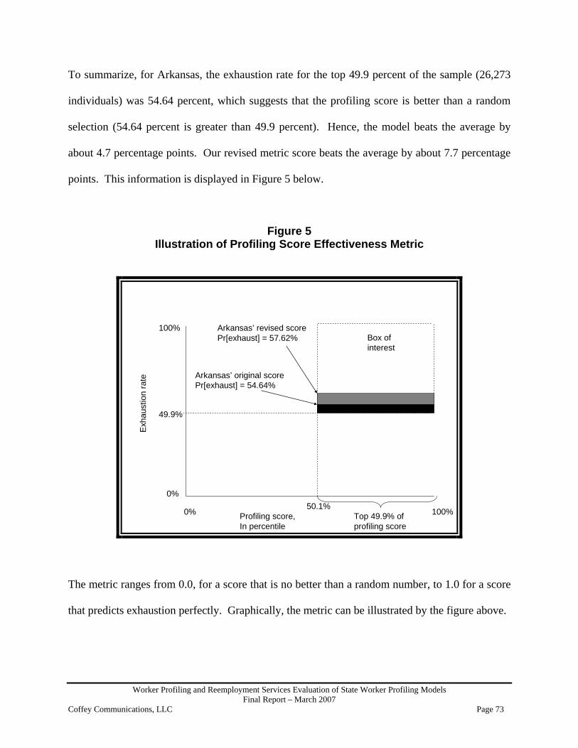
Worker Profiling and Reemployment Services Evaluation of State Worker Profiling Models Final Report – March 2007
Coffey Communications, LLC Page 73
To summarize, for Arkansas, the exhaustion rate for the top 49.9 percent of the sample (26,273
individuals) was 54.64 percent, which suggests that the profiling score is better than a random
selection (54.64 percent is greater than 49.9 percent). Hence, the model beats the average by
about 4.7 percentage points. Our revised metric score beats the average by about 7.7 percentage
points. This information is displayed in Figure 5 below.
Figure 5 Illustration of Profiling Score Effectiveness Metric
Profiling score,In percentile
Exha
ustio
n ra
te
50.1%Top 49.9% of profiling score
49.9%
Box of interest
Arkansas’ original scorePr[exhaust] = 54.64%
Arkansas’ revised scorePr[exhaust] = 57.62%
0%
100%
0% 100%
The metric ranges from 0.0, for a score that is no better than a random number, to 1.0 for a score
that predicts exhaustion perfectly. Graphically, the metric can be illustrated by the figure above.

Worker Profiling and Reemployment Services Evaluation of State Worker Profiling Models Final Report – March 2007
Coffey Communications, LLC Page 74
The figure is a rough illustration that contrasts the profiling score on the X axis, with individuals
ranked from lowest to highest score. On the Y axis is the exhaustion rate of individuals. With
higher profiling scores, we expect the exhaustion rate to increase.
The Box of Interest is the upper right rectangle defined by individuals with percentile profiling
scores above (1.0 minus the state exhaustion rate) and an exhaustion rate above 49.9 percent.
This area represents the set of non-exhaustees expected for a random profiling score.
If the profiling score were a random number, then the metric would be 0. The 49.9 percent of the
sample with the highest profiling score, or 26,273 individuals, would have an exhaustion rate of
49.9 percent. This rate is the same as the state overall. For the sample with the highest profiling
score, 26,273 individuals, 49.9 percent of them would exhaust, or 13,110 individuals. Non-
exhaustees would be 50.1 percent of the 26,273, or 13,163 individuals. This group of 13,163
individuals represents the box of interest. The extent that a profiling score selects these 13,163
as exhaustees determines the value of the metric. For a score that selects all 13,163 as
exhaustees, the metric will have a value of 1.0.
For Arkansas, the original score has a value of 54.64 percent, which is better than the state
exhaustion rate of 49.9 percent. The area under this line, as a percentage of the area of the entire
Box of Interest, is 9.5 percent. This area is shown in the Figure in black.
The revised score has a metric of 0.154, which implies that the area under this line, shown in
Figure 5 above the line for the original score is 15.4 percent of the area in the entire Box of
Interest. The area corresponding to this revised score is shown in the figure as the sum of the
black and gray areas.

Worker Profiling and Reemployment Services Evaluation of State Worker Profiling Models Final Report – March 2007
Coffey Communications, LLC Page 75
For SWAs with hypothetically perfect models, this metric will have a value of 1, and for SWAs
with models that predict no better than random, the metric will take a value of 0. For SWAs to
improve this metric, they would have to develop models that better explain benefit exhaustion,
which is a desirable outcome. This outcome differs from standard measures of goodness of fit
because these focus on explaining non-exhaustion as well as exhaustion. Because this metric
focuses on exhaustion, we think that SWAs will be better able to identify individuals who will
require reemployment services.
In addition to this metric, we also applied the equation below, derived by Silverman, Strange,
and Lipscombe (2004), for calculating the variance ( 2zσ ) of a quotient (p. 1069). This equation
allowed us to calculate the variance for our metric, Z = X/Y, which is the quotient of two random
variables: X (100 - “Pr[Exh]”) and Y (100 - “Exhaustion”). In the equation below, 2Xσ is the
variance of 100 - “Pr[Exh]”, 2Yσ is the variance of 100 - “Exhaustion,” )(XE is the mean for
(100 - “Pr[Exh]”), and )(YE is the mean for (100- “Exhaustion”). By dividing the variance of
the quotient of the two random variables (here 100 - “Exhaustion” and 100 - “Pr[Exh]”) by the
square root of our observations, we were able to determine the standard error of the metric.
Variance of Metric: 4
22
2
22
)()(
)( YEXE
YEYX
zσσ
σ +≈
[X = ( ]Pr[100 Exh− ), Y = ( Exhaustion−100 )]
Standard error of the metric: N
Z2σ
The standard error of our metric is important because it defines the value range for it. For
instance, if our standard error for this dataset was 0.0041, this would imply that the true value for
our metric ranges from a low score of 0.3959 to a high score of 0.4041 with a mean of 0.40.
Larger standard errors indicate more variation in our data and less confidence in our estimates.

Worker Profiling and Reemployment Services Evaluation of State Worker Profiling Models Final Report – March 2007
Coffey Communications, LLC Page 76
The standard error is an important aspect of our analysis because it enables us to compare SWAs
and determine if specific SWAs have models that are significantly better than others. The
standard error enables us to determine significant versus non-significant differences in model
performance.
Applying this metric analysis to the 28 SWAs for which we had data for both profiling score and
exhaustion results in the following table.
Metric for Assessing the Effectiveness of SWA Profiling Scores
SWA Profiling score
Control for endogeneity?
Exhaustion rate for the
state
Number of individuals
with the highest profiling score
Exhaustion rate for
individuals with high profiling scores
Metric Variance of the Metric
Standard Error of
the metric
Arizona original score Y 37.9 21,502 42.8 0.079 1.153 0.007
Arkansas original score N 49.9 26,273 54.6 0.095 1.804 0.008
Arkansas revised score N 49.9 26,273 57.6 0.154 1.686 0.008
Delaware estimated score* N** 39.0 4,207 42.4 0.055 1.227 0.017
District of Columbia
original score N** 56.0 5,385 60.3 0.097 2.277 0.021
District of Columbia
revised score N** 56.0 5,385 63.8 0.176 2.057 0.020
Georgia original score Y 35.7 75,994 44.0 0.129 1.017 0.004
Georgia revised score Y 35.7 75,994 47.3 0.181 0.976 0.004
Hawaii original score Y 39.7 3,526 43.9 0.069 1.248 0.019
Hawaii revised score Y 39.7 3,526 44.8 0.085 1.232 0.019
Idaho estimated score* Y 45.9 15,605 56.1 0.189 1.400 0.009
Idaho revised score Y 45.9 15,605 59.3 0.247 1.306 0.009
Iowa original score Y 15.4 2,456 16.2 0.010 0.368 0.012

Worker Profiling and Reemployment Services Evaluation of State Worker Profiling Models Final Report – March 2007
Coffey Communications, LLC Page 77
Louisiana original score Y 42.6 22,825 51.9 0.161 1.282 0.007
Maine original score Y 37.3 7,346 42.6 0.084 1.121 0.012
Maryland original score N** 50.4 18,974 54.1 0.075 1.877 0.010
Michigan original score Y 52.7 60,128 55.2 0.052 2.110 0.006
Minnesota original score Y 33.6 37,395 43.5 0.150 0.922 0.005
Mississippi original score N 45.5 8,208 47.3 0.033 1.620 0.014
Missouri original score Y 50.6 18,727 58.3 0.156 1.726 0.010
Montana original score Y 53.4 1,678 58.0 0.100 2.051 0.035
Nebraska original score N*** 95.2 44,098 95.5 0.054 36.698 0.029
New Jersey original score Y 62.4 67,030 66.0 0.096 2.947 0.007
New Jersey revised score Y 62.4 67,030 67.6 0.137 2.789 0.006
New York original score Y 40.4 205,729 55.5 0.253 1.073 0.002
Pennsylvania original score Y 46.1 103,172 51.2 0.095 1.564 0.004
Pennsylvania revised score Y 46.1 103,172 52.5 0.118 1.527 0.004
South Dakota original score N** 18.5 1,107 25.6 0.087 0.475 0.021
Tennessee original score Y 49.7 26,299 53.5 0.075 1.830 0.008
Texas original score Y 48.0 190,270 56.6 0.165 1.555 0.003
Texas revised score Y 48.0 190,270 56.9 0.170 1.545 0.003
Vermont original score N** 28.3 359 37.9 0.133 0.756 0.046
Virginia original score Y 23.3 21,186 27.7 0.057 0.611 0.005
West Virginia original score Y 41.0 12,209 50.7 0.164 1.205 0.010
West Virginia updated score Y 41.0 12,209 55.4 0.243 1.109 0.010
Wisconsin original score N 44.2 8,991 46.2 0.036 1.533 0.013
Wyoming original score N** 43.9 47 46.8 0.051 1.497 0.178

Worker Profiling and Reemployment Services Evaluation of State Worker Profiling Models Final Report – March 2007
Coffey Communications, LLC Page 78
* SWA used a characteristic screen. We calculated a profiling score that used the same variables as the screen. ** SWA provided data indicating individuals who were referred, but the effect was insignificant. *** Nebraska had possible data problems, with 95% of the sample having more benefits paid than mba(maximum benefit allowance)
We note that exhaustion of UI benefits is the result of a very complex process that involves the
interaction of individual characteristics and environmental characteristics. None of the models
included enough information to explain a large percentage of exhaustion. The highest value was
.253 for NewYork, a model that only explains 25 percent of exhaustion. However, our
development of a metric allows SWAs to compare the effectiveness of different versions of their
models.
Step 8 - Analyze the Variables that Appear to Best Reduce Type I Errors or Improve the
Performance of the Model for Individuals with High Profiling Scores
Thus far, we have discussed the models we used in our analysis of the SWA-provided data. This
discussion has included how well, on average, the original models performed, how introducing
additional information from the dataset can possibly improve the proper classification of
potential benefit exhaustees, and how we gauged improvements between the original model used
by the SWA and the models we created for the data provided. There is, however, one important
piece missing from this discussion – how we determine which variables are important in
explaining the differences between benefit exhaustees and non-exhaustees.
Below is STATA output from an example dataset we created to explain the difference between
benefit exhaustees and non-exhaustees using job tenure. We found that for this example dataset,
there is a difference in the means of job tenure between benefit exhaustees and non-exhaustees.
As detailed below, there were 655 benefit recipients who did not exhaust benefits, and 1,023 that
did. Here we found that non-exhaustees had a mean of approximately 5.096 years at their

Worker Profiling and Reemployment Services Evaluation of State Worker Profiling Models Final Report – March 2007
Coffey Communications, LLC Page 79
previous employer. For exhaustees the mean for job tenure was approximately 5.957 years, a
difference of approximately 0.861 years. We apply the following equation, as detailed in our
STATA output, to determine the difference between the two means:
Difference = mean(non-exhaustees) – mean(exhaustees)
Group Observations Mean Standard
Error Standard Deviation
[95% Conf. Interval]
Non-Exhaustees
655 5.096183 .3163604 8.096601 4.474979 5.717388
Exhaustees 1023 5.957967 .2839745 9.082746 5.400727 6.515206 Combined 1678 5.621573 .2128432 8.718779 5.204107 6.03904 Difference -.8617836 .4359302 -1.716809 -.0067586
Difference = mean(non-exhaustees) – mean(exhaustees) Z-score = -1.9769 Ho: difference = 0 degrees of freedom = 1676 Ha: difference < 0 Ha: difference != 0 Ha: difference > 0 Pr(T < t) = 0.0241 Pr(T > t) = 0.0482 Pr(T > t) = 0.9759 As detailed in our STATA output, our null hypothesis here is that there is no difference between
the two groups of benefit recipients. However, as shown in our STATA output, we reject this
null hypothesis and accept that the alternative hypothesis (that the means for the two groups are
not same) is true. We determine this by looking at the associated P-values for our null
hypotheses. As we can see from our STATA output, the difference between the two means is
not zero and has a corresponding P-value of 0.0482. This implies that we are at least 95 percent
confident that the difference between the two means is not zero.
We do not include the above table for each variable t-test we performed; however, we include
the corresponding P-value, the means for each group, and the Z-score used to determine the
significance level (or P- value ) for each variable. By testing for differences in means for the two

Worker Profiling and Reemployment Services Evaluation of State Worker Profiling Models Final Report – March 2007
Coffey Communications, LLC Page 80
groups, we hope to provide a way for SWAs to determine variables (whether they be categorical
or continuous) that are important for explaining the difference between exhaustees and non-
exhaustees.
An In-Depth Analysis of the Wage Replacement Rate Variable
Based on the analyses in Appendix D, one of the more powerful variables currently used in
WPRS profiling models is the wage replacement rate. However, it is important to note that
currently only 15 SWAs use this as a variable. The wage replacement rate measures the
proportion of a claimant’s wages that are replaced by unemployment insurance (UI) payments.
For example, if a claimant received $400 per week prior to filing a UI claim and the claimant
receives $240 per week in UI payments, the wage replacement rate is 0.60. For a number of
reasons the wage replacement rate is an interesting variable. Chief among them is that it is
significant in predicting the probability of exhaustion (Pr[exh]) both as a categorical variable and
as a continuous variable.
In our analysis for Arizona, we defined the wage replacement rate for claimants by multiplying
the ratio of the weekly benefit amount to base period wages by 52 (the number of weeks in a
year) as detailed below.
52 WagesPeriod Base
AmountBenefit Weekly Ratet Replacemen Wage ×=
In doing so we found a range of values for the wage replacement rate: from 0.0019202 to
1.978378 (we ignored all wage replacement rates above 2.0). As detailed in our analysis on the
2003 Arizona data, we first used the wage replacement rate in our updated model as a categorical
variable. From our analysis, we found that wage replacement rate was significant, particularly
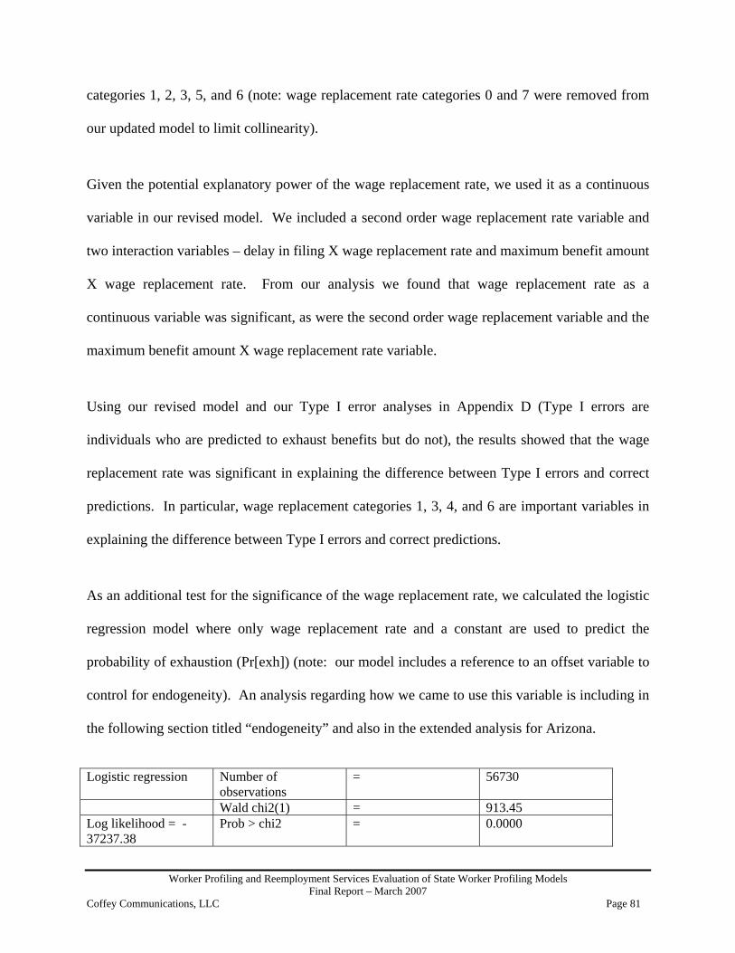
Worker Profiling and Reemployment Services Evaluation of State Worker Profiling Models Final Report – March 2007
Coffey Communications, LLC Page 81
categories 1, 2, 3, 5, and 6 (note: wage replacement rate categories 0 and 7 were removed from
our updated model to limit collinearity).
Given the potential explanatory power of the wage replacement rate, we used it as a continuous
variable in our revised model. We included a second order wage replacement rate variable and
two interaction variables – delay in filing X wage replacement rate and maximum benefit amount
X wage replacement rate. From our analysis we found that wage replacement rate as a
continuous variable was significant, as were the second order wage replacement variable and the
maximum benefit amount X wage replacement rate variable.
Using our revised model and our Type I error analyses in Appendix D (Type I errors are
individuals who are predicted to exhaust benefits but do not), the results showed that the wage
replacement rate was significant in explaining the difference between Type I errors and correct
predictions. In particular, wage replacement categories 1, 3, 4, and 6 are important variables in
explaining the difference between Type I errors and correct predictions.
As an additional test for the significance of the wage replacement rate, we calculated the logistic
regression model where only wage replacement rate and a constant are used to predict the
probability of exhaustion (Pr[exh]) (note: our model includes a reference to an offset variable to
control for endogeneity). An analysis regarding how we came to use this variable is including in
the following section titled “endogeneity” and also in the extended analysis for Arizona.
Logistic regression Number of
observations = 56730
Wald chi2(1) = 913.45 Log likelihood = -37237.38
Prob > chi2 = 0.0000

Worker Profiling and Reemployment Services Evaluation of State Worker Profiling Models Final Report – March 2007
Coffey Communications, LLC Page 82
exhaust Coefficient Standard error
z P>z [95% Conf. Interval]
wrr .8756011 .028971 30.22 0.000 .818819 .9323832 _cons -.9980725 .0193361 -51.62 0.000 -1.03597 -.9601745 endogeneity control
(offset)
As we can see from the associated low P-value, wage replacement rate does have a significant
impact on predicting the probability of benefit exhaustion. For a comparison we will look at the
predicted probability score that Arizona provided us and the corresponding wage replacement
rate for that claimant. Using the coefficients from the above calculations we will first calculate
the score using the wage replacement rate, the corresponding coefficient, and the constant.
Z = wrr*(0.8756011) – 0.9980725 Z = (0.6155989)*(0.8756011) – 0.9980725 Z = -0.45905342600121
Next, we use this value, Z, in the following logistic regression transformation to determine the
predicted probability of benefit exhaustion.
Pr[exh] = 1+Z
Z
ee = 0.38721
The probability score provided by Arizona for the claimant with a wage replacement rate of
0.6155989 was 0.13552. From our detailed analysis for the 2003 Arizona data, our predicted
probability score for this claimant was 0.3842769. This score was calculated using only the
score provided by Arizona along with a constant (we included the offset variable in our model to
control for endogeneity). The predicted probability score for this claimant for our updated model
was 0.4769786 and 0.4805083 for our revised model.
Worker Profiling and Reemployment Services Evaluation of State Worker Profiling Models Final Report – March 2007
Coffey Communications, LLC Page 83
CONCLUSION: BEST PRACTICES IN WPRS MODELS
FOR PREDICTING EXHAUSTION OF UI BENEFITS
For this study, we collected information that describes how SWAs operate their models for
predicting exhaustion of UI benefits and refer individuals for reemployment services, and we
analyzed the models used by SWAs to predict exhaustion. The descriptions of SWA operations
are contained in Part 3 above and Appendices B and C, and demonstrate the variety of
approaches used by SWAs for profiling. In terms of best practices, our analyses suggest that
SWAs can improve their models by including more information, including introducing more
variables and including second-order effects.
The profiling models currently operate in terms of their ability to properly classify benefit
exhaustees. As a part of our task, we have performed updates and revisions to the provided
profiling models and analyzed the results to determine if there are ways to improve the profiling
power of the models. We think that there are methods and variables that SWAs can incorporate
into their current profiling models to improve performance. A more effective model also will
reduce staff effort and help ensure the effective application of valuable reemployment services.
Depending on the SWA and dataset, incorporating continuous variables, such as job tenure and
education and second order variables (i.e., variables that are centered and squared) improved the
predictions of the profiling models. Furthermore, introducing cross-term variables, i.e., variables
that are the product of two centered continuous variables, also led to an improvement.

Worker Profiling and Reemployment Services Evaluation of State Worker Profiling Models Final Report – March 2007
Coffey Communications, LLC Page 84
From our analyses of the profiling models and datasets for nine SWAs (Arkansas, the District of
Columbia, Georgia, Hawaii, Idaho, New Jersey, Pennsylvania, Texas, and West Virginia), we
found that the following features generally helped to properly classify potential benefit
exhaustees:
• Using a logistic regression model
• Including the following independent variables:
o Maximum Benefit Amount
o Wage Replacement Rate
o Potential Duration of Benefits
o Education Level
o Delay in Filing for UI Benefits
o Benefit Exhaustion Rate for Prior Industry
o County Unemployment Rate
o County/Metro Area of Residence
o Industry and Occupation Codes
• Including continuous variables
• Including second-order and cross-term variables if more than one continuous variable is
included in the model
Including the wage replacement rate of claimants is significant in explaining the differences
between exhaustees and non-exhaustees; moreover, wage replacement rate also has the
distinction of being significant as both a categorical variable and as a continuous variable. The
same is true of the maximum benefit amount and job tenure, though the significance of each is
determined by how their categories are defined.

Worker Profiling and Reemployment Services Evaluation of State Worker Profiling Models Final Report – March 2007
Coffey Communications, LLC Page 85
REFERENCES Amemiya (1973). Regression analysis when the dependent variable is truncated normal. Econometrica, 41: 997-1016. Anderson, P., Corson, W., & Decker, P. (1991). The New Jersey Unemployment Insurance Reemployment Demonstration Project: Follow-Up Report. UI Occasional Paper 91-1. Washington, DC: U.S. Department of Labor. Balducci, David E., Randall W. Eberts, Christopher J. O’Leary, eds. 2004. Labor Exchange Policy in the United States. Kalamazoo, MI: W.E. Upjohn Institute for Employment Research. Benus, Jacob M., Terry R. Johnson, Michelle Wood, Neelima Grover, and Theodore Shen. 1994. Self-Employment Programs: A New Reemployment Strategy. Final Impact Analysis of the Washington and Massachusetts Self-Employment Demonstrations. Washington, DC: Department of Labor, Employment and Training Administration. Berger, Mark C., Dan A. Black, Amitabh Chandra, and Steven N. Allen. 1997. “Profiling Workers for Unemployment Insurance in Kentucky.” The Kentucky Journal of Business and Economics 16: 1-18. Black, Dan A., Jeffrey A, Smith, Miana Plesca, and Suzanne Plourde. 2002. Estimating the Duration of Unemployment Insurance Benefit Recipiency. Final Technical Report. Contract Number UI-10909-00-60. Washington, DC: Department of Labor, Employment and Training Administration. Black, Dan A., Jeffrey A. Smith, Mark C. Berger, Brett J. Noel. 2003. “Is the Threat of Reemployment Services More Effective than the Services Themselves? Evidence from Random Assignment in the UI System.” The American Economic Review 93(4): 1317-1327. Black, Dan A., Jeffrey A. Smith, Miana Plesca, and Suzanne Shannon. 2003. Profiling UI Claimants to Allocate Reemployment Services: Evidence and Recommendations for States. Final Report. Washington, DC: Department of Labor, Employment and Training Administration. Camilli, G. & Congdon, P. (1999). Application of a method of estimating DIF for polytomous test items. Journal of Educational and Behavioral Statistics, 24 (4): 323-341. Camilli, G. & Shepard, L. A. (1994). Methods for Identifying Biased Test Items. Newbury Park, CA: Sage Publications. Corson, Walter, Paul T. Decker, Shari Miller Dunstan, and Anne R. Gordon, 1989. The New Jersey Unemployment Insurance Reemployment Demonstration Project. Unemployment Insurance Occasional Paper 89-3. Washington, DC: Department of Labor, Employment and Training Administration.

Worker Profiling and Reemployment Services Evaluation of State Worker Profiling Models Final Report – March 2007
Coffey Communications, LLC Page 86
Corson, Walter and Joshua Haimson. 1996. The New Jersey Unemployment Insurance Reemployment Demonstration Project: Six-year Follow-up and Summary Report, Unemployment Insurance Occasional Paper 96-2. Washington, DC: Department of Labor, Employment and Training Administration. Corson, Walter and Paul T. Decker. 1996. “Using the Unemployment Insurance System to Target Services to Dislocated Workers,” in Advisory Council on Unemployment Compensation, Background Papers, Volume III. Washington, DC: U. S. Department of Labor. Davidson, R. and MacKinnon, J. (1993). Estimation and Inference in Econometrics. New York: Oxford University Press. Decker, Paul T., Robert B. Olsen, Lance Freeman and Daniel H. Klepinger. 2000. Assisting Unemployment Insurance Claimants: The Long Term Impacts of the Job Search Assistance Demonstration. Mathematica Policy Research, Inc. Contract Number M-4361-00-97-30. Washington, DC: U. S. Department of Labor, Employment and Training Administration. Dickinson, Katherine P., Paul T. Decker, and Suzanne D. Kreutzer. 1997. Evaluation of Worker Profiling and Reemployment Services Systems: Report to Congress. Washington, DC: Office of Policy and Research, U.S. Department of Labor, Employment and Training Administration. Dickinson, Katherine P., Paul T. Decker, Suzanne D. Kreutzer, and Richard W. West. 1999. Evaluation of Worker Profiling and Reemployment Services: Final Report. Research and Evaluation Report Series 99-D. Washington, DC: Office of Policy and Research, U.S. Department of Labor, Employment and Training Administration. Dickinson, Katherine P., Paul T. Decker, Suzanne D. Kreutzer. 2002. “Evaluation of WPRS Systems,” in Randall W. Eberts, Christopher J. O’Leary, Stephen A. Wandner, eds. Targeting Employment Services. Kalamazoo, MI: W.E. Upjohn Institute for Employment Research. Eberts, Randall W. and Christopher J. O’Leary. 2003. A New WPRS Profiling Model for Michigan. Prepared for the Michigan Bureau of Workers’ and Unemployment Compensation. Upjohn Institute Staff Working Paper No. 04-102. Kalamazoo, MI: W.E. Upjohn Institute for Employment Research. Eberts, Randall W. (2002). Design, Implementation, and Evaluation of the Work First Profiling Pilot Project. UI Occasional Paper 2002-07. Washington, DC: U.S. Department of Labor. Eberts, Randall W. and Christopher J. O’Leary. 2004. “Personal Reemployment Accounts.” Employment Research (January). Eberts, Randall W. and Christopher J. O’Leary. 1997. “Profiling and Referral to Services of the Long-Term Unemployed: Experiences and Lessons Learned from Several Countries.” Employment Observatory: Policies (inforMISEP), 60, Berlin: Institute for Applied Socio-Economics (Winter).

Worker Profiling and Reemployment Services Evaluation of State Worker Profiling Models Final Report – March 2007
Coffey Communications, LLC Page 87
Eberts, Randall W. and Christopher J. O’Leary. 1996. “Profiling Unemployment Insurance Beneficiaries.” Employment Research (October). Eberts, Randall W., Christopher J. O’Leary, Stephen A. Wandner. 1999. “Targeting Employment Services Conference.” Employment Research (April). French, A. W. & Miller, T. R. (1996). Logistic regression and its use in detecting differential item functioning in polytomous items. Journal of Educational Measurement, 33 (3): 315-332. Hawkins, Evelyn K., Suzanne D. Kreutzer, Katherine P. Dickinson, Paul T. Decker, and Walter S. Corson. 1996. Evaluation of Worker Profiling and Reemployment Systems: Interim Report. UI Occasional Paper 96-1. Washington, DC: U.S. Department of Labor, Employment and Training Administration, Unemployment Insurance Service. Johnson, Terry R. 1996. “Reemployment Service Strategies for Dislocated Workers: Lessons Learned from Research,” Worker Profiling and Reemployment Services (WPRS) System: National WPRS Colloquium: Selected Papers and Materials. Washington, DC: U.S. Department of Labor, Employment and Training Administration. Kelso, Marisa L. 1998. “Worker Profiling and Reemployment Services Profiling Methods: Lessons Learned.” UI Research Exchange. UI Occasional Paper 99-5. Washington, DC: U.S. Department of Labor, Employment and Training Administration, Unemployment Insurance Service, Division of Research and Policy. Kosanovich, William T., Heather Fleck, Berwood Yost, Wendy Armon, Sandra Siliezar. 2001. Comprehensive Assessment of Self-Employment Assistance Programs: Final Report. Contract Number F-6829-8-00-80-30. Washington, DC: Department of Labor, Employment and Training Administration. Maddala, G. S. (1983). Limited-Dependent and Qualitative Variables in Econometrics. Cambridge: Cambridge University Press. Messenger, Jon C., Carolyn Peterson Vaccaro, and Wayne Vroman. 1999. “Profiling in Self-Employment Assistance Programs.” Targeting Employment Services Conference Paper. Kalamazoo, MI. Meyer, Bruce D. 1995. “Lessons from the U.S. Unemployment Insurance Experiments.” Journal of Economic Literature, 33 (March): 91-131. Needels, Karen, Walter Corson, Walter Nicholson. 2001. Left Out of the Boom Economy: UI Recipients in the Late 1990s. Mathematica Policy Research, Inc. Contract Number M-7042-8-00-97-30. Washington, DC: U. S. Department of Labor, Employment and Training Administration. Needels, Karen, Walter Corson, Michelle Van Noy. 2002. Evaluation of the Significant Improvement Demonstration Grants for the Provision of Reemployment Services for UI

Worker Profiling and Reemployment Services Evaluation of State Worker Profiling Models Final Report – March 2007
Coffey Communications, LLC Page 88
Claimants: Final Report. Mathematica Policy Research, Inc. Contract Number F-6828-8-80-30(06). Washington, DC: U. S. Department of Labor, Employment and Training Administration. O’Leary, Christopher J., Paul Decker, and Stephen A. Wandner. 1997. Reemployment Bonuses and Profiling. Upjohn Institute Staff Working Paper No. 98-51. Kalamazoo, MI: W.E. Upjohn Institute for Employment Research. O’Leary, Christopher J., Stephen A. Wandner, eds. 1997. Unemployment Insurance in the United States. Kalamazoo, MI: W.E. Upjohn Institute for Employment Research. O’Leary, Christopher J. 2006. “State UI Job Search Rules and Reemployment Services.” Monthly Labor Review, 129(6). O’Leary, Christopher J. 2004. “Evaluating the Effectiveness of Labor Exchange Services,” in David E. Balducchi, Randall W. Eberts and Christopher J. O’Leary, eds. Labor Exchange Policy in the United States. Kalamazoo, MI: W.E. Upjohn Institute for Employment Research. O’Leary, Christopher J. 1998. “Profiling for Reemployment Bonus Offers.” Employment Research (April.) O’Leary, Christopher J. 2003. Testimony before the Subcommittee on Income Security and Family Support of the House Committee on Ways and Means (April). Olsen, Robert B., Marisa Kelso, Paul T. Decker, Daniel H. Klepinger. 2002. “Predicting the Exhaustion of Unemployment Compensation,” in Randall W. Eberts, Christopher J. O’Leary, Stephen A. Wandner, eds. Targeting Employment Services. Kalamazoo, MI: W.E. Upjohn Institute for Employment Research. Organisation for Economic Co-operation and Development (OECD). 1998. Early Identification of Job Seekers at Risk of Long-Term Unemployment: The Role of Profiling. Paris: Organisation for Economic Co-operation and Development. Silverman, M. P., Strange, W. & Lipscombe, T.C. (2004). The distribution of composite measurements: How to be certain of the uncertainties in what we measure. American Journal of Physics, 72(8), 1068-1081. Swaminathan, H. & Rogers, H. J. (1990). Detecting differential item functioning using logistic regression procedures. Journal of Educational Measurement, 27 (4): 361-370. Tobin, J. (1958). Estimation of relationships for limited dependent variables. Econometrica, 26: 601-8. Unemployment Compensation Amendments of 1993 (1993). Pub. L. No. 103-152, 107 Stat. 1516.

Worker Profiling and Reemployment Services Evaluation of State Worker Profiling Models Final Report – March 2007
Coffey Communications, LLC Page 89
U.S. Department of Labor, Employment and Training Administration. 1994. The Worker Profiling and Reemployment Services System: Legislation, Implementation Process, and Research Findings, Unemployment Insurance Occasional Paper 94-4. Washington, D.C. U.S. Department of Labor. (1995). What’s Working (and what’s not): A Summary of Research of the Economic Impacts of Employment and Training Program. Washington, DC: Office of the Chief Economist. Wandner, Stephen A. 2002. “Targeting Employment Services under the Workforce Investment Act,” in Randall W. Eberts, Christopher J. O’Leary, Stephen A. Wandner, eds. Targeting Employment Services. Kalamazoo, MI: W.E. Upjohn Institute for Employment Research. Wandner, Stephen A., and Jon C. Messenger, eds. 1999. Worker Profiling and Reemployment Services Policy Workgroup: Final Report and Recommendations. Washington, DC: U. S. Department of Labor, Employment and Training Administration. Wisconsin Department of Workforce Development. (2006). UI Reemployment Services. Retrieved October 16, 2006 from http://www.dwd.state.wi.us/dws/bjs/Reemployment.htm. Woodbury, Stephen A. 2000. “New Directions in Reemployment Policy.” Employment Research (October). Worden, Kelleen. 1993. “Profiling Dislocated Workers for Early Referral to Reemployment Services,” UIS Information Bulletin No. 4-91, in U. S. Department of Labor, Employment and Training Administration. 1994. The Worker Profiling and Reemployment Services System: Legislation, Implementation Process, and Research Findings, Unemployment Insurance Occasional Paper 94-4. Washington D.C.

Worker Profiling and Reemployment Services Evaluation of State Worker Profiling Models Final Report – March 2007
Coffey Communications, LLC Page 90
APPENDICES

Worker Profiling and Reemployment Services Evaluation of State Worker Profiling Models Final Report – March 2007
Coffey Communications, LLC Page 91
APPENDIX A
SURVEY INSTRUMENT

Worker Profiling and Reemployment Services Evaluation of State Worker Profiling Models Final Report – March 2007
Coffey Communications, LLC Page 92
Worker Profiling Reemployment Services (WPRS) Survey
(Operational Section) Please enter the name of your State: 1. Please provide the name, title, e-mail address, and phone number of the individual(s) completing
this survey including which survey questions they completed: 2. Please provide the name, title, e-mail address, and phone numbers of the individuals within UI, ES
(Workforce Development), LMI, and IT who provide daily control and oversight of the WPRS process and model (if different from above).
3. How frequently is the model updated (run to generate new statistical parameters)?
Yearly ___________ 2-3 Years ___________ More than 3 Years ___________ Other ___________
3a. Date of Last Update: _________________________ 4. Has the model been revised (i.e., other than update, has the model been revised in any way, such
as a change in the variables used, the variable definitions, or functional form) since implementation?
Yes _______ No _______
4a. If Yes, please provide date of last revision and brief description of revisions made: 4b. Do you have policy guidance to revise your model and if so, how often? Is there a decision maker
within your agency who determines that the model will be revised? 5. By which method(s) is your initial claim process performed? (check all that apply and estimate
percentages)
In-Person ________ By Telephone ________ By Mail ________ Internet ________ Other:(specify) ____________________________________________________ ____________________________________________________
6. Are all of the claimant “characteristics” data needed for profiling purposes captured at the time of
the initial claim?
Yes ________ No ________

Worker Profiling and Reemployment Services Evaluation of State Worker Profiling Models Final Report – March 2007
Coffey Communications, LLC Page 93
6a. If you answered “No” above, please describe how, and when, the data are captured or generated: 6b. Are there any checks on the accuracy of claimant provided information?
Yes ________ (If Yes, Please describe below) No ________
7. How frequently is the WPRS model run?
Daily ___________ Weekly ___________ Other (please describe) _________________________________________________ ____________________________________________________________________
7a. Is the listing of profiling candidates produced at the same time the model is run?
Yes ________ No ________
If “No,” please describe when the listing is produced: ________________________________________________________________________ ________________________________________________________________________
8. Is the model run against the first pay records?
Yes ________ No ________
8a. If you answered “No” to question 8, please describe against what UI or other data the model is run.
________________________________________________________________________________________________________________________________________________________________________________________________
9. Who determines and assigns the claimant’s occupational code?
Initial Claims Taker __________ Workforce Dev. Worker __________ Other (please describe) _____________________________________________ ____________________________________________________________________
9a. Which occupational coding system is used (DOT, SOC or, if any other classification system is
used, please identify)? 9b. How is the occupational code derived for the claimant? (please describe, if not a standard
classification system) 10. How is the claimant’s primary employer (for assigning NAICS/SIC code) determined?
Review of work history with claimant _________

Worker Profiling and Reemployment Services Evaluation of State Worker Profiling Models Final Report – March 2007
Coffey Communications, LLC Page 94
Review of wage records ________ Other (please describe) ____________________________________________________ _________________________________________________________________________
11. Who is exempt from profiling in your State? 12. To whom is the list of profiling candidates sent, and using what medium? (describe) 13. Who determines the number of profiled candidates to be served and how is the number
determined? 14. How do the probability scores, or rankings, influence selection of candidates from the pool? 15. Under what conditions can the local area skip down ranks in selecting candidates for services? 16. Are there feedback loops in place between local area operations and the WPRS model builders?
Yes ________ No ________
17. The original parameters for WPRS suggested individuals who had received more than 5 weeks of
benefits prior to selection be excluded from the pool (e.g. if payment delays have deferred first payments for more than five weeks). Is this parameter in place in your system?
Yes ________ No ________ If No, please provide the number you use
18. Has the accuracy of data needed for the Characteristic Screens been measured or tested to compare
it to the predictive equation approach or has the existence of missing or inaccurate data been investigated?
Yes ________ (If Yes, please describe results below) No ________
19. Has your agency conducted any studies to evaluate the accuracy of the profiling model in
predicting who will exhaust benefits? Yes ________ (If Yes, please describe below) No ________
(Structural Section)
SOME STATES MAY FIND IT ADVANTAGEOUS TO SIMPLY ATTACH TECHNICAL REPORTS OR COMPUTER PRINT-OUTS TO REPLY TO THE HIGHLY TECHNICAL STRUCTURAL QUESTIONS (especially 24, 25, 26, & 31). PLEASE BE SURE TO ATTACH THE REPORTS AND EXPLAIN WHERE IN THE REPORT OR PRINTOUT THE PERTINENT MATERIAL MAY BE FOUND.
Please note all questions that follow apply to the model that was primarily in use during the period _____________ to ___________.
20. Which type of WPRS Model does your state currently use? Enter “Yes” in appropriate block.
Characteristic Screen __________

Worker Profiling and Reemployment Services Evaluation of State Worker Profiling Models Final Report – March 2007
Coffey Communications, LLC Page 95
Statistical Model __________ 20a. What is your model’s functional form? (example: logit, probit, tobit, linear, characteristic screen,
other). 21. Which individuals are included in the data when the model was first estimated, or when it was
updated or revised?
All initial claim filers _______ Only benefit recipients ________ Union member _______ Others not profiled (describe) ____________________________________________ ____________________________________________________________________
21a. What is the sample size in the model’s latest update and what was the original sample size when
the model was first estimated? 22. What is your model’s dependent (left-hand side) variable?
Exhaustion ________Duration of Benefits________ Both ________ Other (describe) _______________________________________________________ ____________________________________________________________________
23. For the purpose of updating your model, how do you define exhaustion of benefits? (check all
options which apply)
Maximum benefits paid __________ Received 26 weekly payments ________ Benefit payments denied but under appeal ________ Other(describe) ____________________________________________________________________ ____________________________________________________________________
24. What are your model’s independent (right-hand side) variables and how are they defined? Please
include and explain how to calculate the variables and explain what data are used to create the variable. (examples: maximum duration = maximum benefit amount divided by weekly benefit amount; example 2: industry = the first digit of the NAICS hierarchical code). If you use a characteristic screen, what characteristics do you use?
_______________________________________________________________________ _______________________________________________________________________
25. What determined the selection of the independent (right-hand side) variables used in the predictive
equation? Were any other variables examined?
_______________________________________________________________________ _______________________________________________________________________

Worker Profiling and Reemployment Services Evaluation of State Worker Profiling Models Final Report – March 2007
Coffey Communications, LLC Page 96
25a. What are the numerical values of the estimated coefficients for the independent (right-hand side) variables and if this information is readily available, what was the standard error for each? (This information should be found on the original statistical output for the original estimation technique.)
_______________________________________________________________________ _______________________________________________________________________
26. What techniques are followed to prepare a claims data record for profiling using the equation?
(e.g., are there checks for missing values, are union member claims profiled, are there data quality checks, etc.)
________________________________________________________________ _______________________________________________________________________
27. How are claimants with incomplete records, or records with missing variables, processed? (check
all that apply)
_____ a. variable kept blank and a binary variable used to track the missing variable _____ b. another version of the profiling model used _____ c. value of missing data estimated by some other procedure _____ d. missing value replaced by average value for the individuals in the run or
some other average value _____ e. Other method? (please describe)
28. Were the exclusion rules (see question 11) applied to the data records used during the estimation of
the predictive equation? That is, were records excluded from the estimation database, and what percentage of claimants is excluded from profiling? _______________________________________________________________________
_______________________________________________________________________ 29. Were the data quality procedures that were used for the data in the estimation of the predictive
equation different from those used now for profiling? If so, how? In your view, does the elimination of claim records as a result of data quality procedures have an effect (either negative or positive) on the performance of the equation?
_______________________________________________________________________
_______________________________________________________________________ 30. Are the predicted values of the dependent (left-hand side) variables retained in electronic storage
archives? Yes _______ No _______
31. What are the ranges of permissible (or expected) values of the data for the independent (right-hand
side) variables (minimum and maximum)? Please describe below.

Worker Profiling and Reemployment Services Evaluation of State Worker Profiling Models Final Report – March 2007
Coffey Communications, LLC Page 97
APPENDIX B
COMPARISON TABLE OF SWA WPRS MODELS

Worker Profiling and Reemployment Services Evaluation of State Worker Profiling Models Final Report – March 2007
Coffey Communications, LLC Page 98
Structural/Operational Methods of Initial Filing
(percentage, if available) Model Run Information Model Use Information
SWA
Mod
el T
ype
Func
tiona
l For
m
Freq
uenc
y of
Upd
ate
Dat
e of
Las
t Upd
ate
Mod
el R
evis
ion
In P
erso
n
Tel
epho
ne
Mai
l
Inte
rnet
Freq
uenc
y of
Mod
el
Run
Mod
el R
un A
gain
st?
Whe
n C
andi
date
Lis
t Pr
oduc
ed?
Occ
upat
iona
l Cod
ing
Syst
em
Prim
ary
Em
ploy
er
Ass
ignm
ent
To
Who
m C
andi
date
L
ist S
ent
# to
be
Serv
ed
Det
erm
ined
By
Dis
cret
ion
in S
elec
t. Pa
rtic
ipan
ts
Alabama 1 statistical logit 2-3 yrs none 2000 X weekly
first pay
records time of run SOC wage
records
career centers using the
Alabama Job Link Sys.
career centers based on their
capacity No
Alaska statistical logit yearly 01/06 01/05 92% 8% weekly
first pay
records time of run DOT/SOC
work history/wage
records
employment services provider
employment services unit No
Arizona statistical INA 2-3yrs 07/03 07/03 X X X daily
first pay
records
when requested
by orientation provider INA
last employer
orientation provider
program manager No
Arkansas statistical
linear (multiple
regression) >3 yrs never none X X weekly
first pay
records time of run DOT wage
records
Job Search Workshop
Coordinators
workshop coordinators
based on capacity
No, unless an higher ranked
candidate cannot be contacted
California statistical logit >3 yrs 12/01 none 60% 5% 35% weekly
first pay
records time of run DOT/SOC
work history/wage
records
Employment Service
Scheduling System
Field Office Manager or
IAW Workshop
Leader No
Colorado statistical logit never never never 80% 20% weekly
first pay
records time of run SOC wage
records workforce
center workforce
center Yes
Connecticut statistical neural
network never never never 91.1% 8.9% weekly
first pay
records time of run ONET/SOC none
State Department of
Labor Staff
State Department of
Labor Job Center
Directors
Yes, if the claimant has
returned to work or moved out of
state
Delaware characteristic screen NA >3 yrs never never X X weekly
at first pay
record time of run ONET/SOC work history
Division of Employment and Training
Division of Employment and Training No
District of Columbia 2 statistical logit 2-3 yrs 01/04 10/04 20% 80% weekly
at first pay
records time of run ONET wage
records
One Stop Management
Staff
One Stop Management
Staff No
Florida
no scoring - regional boards decided those most likely to exhaust INA INA none 01/02 45% 5% 50% weekly
at first pay
records time of run ONET work history
One Stop Management
Staff
One Stop Management
Staff Yes
Georgia statistical logit >3yrs 01/98 never X daily
at intake
process time of run DOT
work history/wage
records Employment
Services Career Center
Managers
Yes, for non- mandatory participants
Hawaii statistical logit >3yrs 01/95 01/02 10% 90% weekly
at first pay
record time of run SOC work history UI/WDD/R&S
Workforce Development
Division Yes, only for rescheduling
Idaho characteristic screen characteristic yearly 05/05 05/05 5% 6% 89% weekly
at first pay
record time of run SOC wage
records local
consultants
Office management
staff Yes

Worker Profiling and Reemployment Services Evaluation of State Worker Profiling Models Final Report – March 2007
Coffey Communications, LLC Page 99
Structural/Operational Methods of Initial Filing (percentage, if available) Model Run Information Model Use Information
SWA
Mod
el T
ype
Func
tiona
l For
m
Freq
uenc
y of
Upd
ate
Dat
e of
Las
t Upd
ate
Mod
el R
evis
ion
In P
erso
n
Tel
epho
ne
Mai
l
Inte
rnet
Freq
uenc
y of
Mod
el
Run
Mod
el R
un A
gain
st?
Whe
n C
andi
date
Lis
t Pr
oduc
ed?
Occ
upat
iona
l Cod
ing
Syst
em
Prim
ary
Em
ploy
er
Ass
ignm
ent
To
Who
m C
andi
date
L
ist S
ent
# to
be
Serv
ed
Det
erm
ined
By
Dis
cret
ion
in S
elec
t. Pa
rtic
ipan
ts
determine yearly target
number
Illinois statistical logit other 1997 none 80% 20% weekly
first pay
records time of run DOT wage
records
Local Workforce Investment
Area
Local Workforce Investment
Area No
Indiana statistical linear
regression never never none X X weekly
at first pay
record time of run DOT work history local office
staff local office managers No
Iowa statistical logit never never none 46% 31% 19% weekly
first pay
records
at orientation selection SOC/DOT
last employer
local profiling coordinators
UI/Workforce Development administration No
Kansas statistical logit never never none 75% 25% daily
first pay
records time of run SOC work history
local workforce
development offices
workforce development
staff determined by
workload No
Kentucky statistical tobit >3yrs 01/97 none X X X weekly
first pay
records time of run OES wage
recodes local office
staff
Director of the Division for Workforce
and Employment
Svcs. No
Louisiana statistical logit 3-5 yrs 06/03 06/03 5% 95% weekly
first pay
records time of run ONET/SOC work history
Wagner/Peyser and WIA staff via mainframe
local office staff based on
capacity Yes, at will
Maine statistical logit >3yrs 9/04 01/00 X X X weekly
first pay
records time of run DOT wage
records
Employment Services and
then to Career Centers
Career center determined by
capacity No
Maryland statistical logit >3yrs 01/00 none X X weekly
first pay
records time of run DOT wage
records
WPRS workshop facilitators
WPRS workshop facilitators
determined by space
available No
Massachusetts characteristic screens characteristic other never 05/05 X weekly
first pay
records
following screening
of first payments
claimant determines
last employer
ES system for tracking WIA service and outcomes INA INA
Michigan statistical linear
regression >3yrs 6/03 6/03 X X X weekly
first pay
records time of run SOC wage
records
Workforce Development Board (WDB) Coordinator
Each WDB determined by resources and
staffing
Yes, but only for candidates below
the mandatory rank
Minnesota statistical logit 2-3yrs 05/05 05/05 55% 5% 40% daily
first claim data time of run DOT/SOC work history
Resource Area Coordinators
Resource Area Coordinators Yes
Mississippi statistical INA never never none 100% weekly first the day SOC work history workforce workforce INA

Worker Profiling and Reemployment Services Evaluation of State Worker Profiling Models Final Report – March 2007
Coffey Communications, LLC Page 100
Structural/Operational Methods of Initial Filing (percentage, if available) Model Run Information Model Use Information
SWA
Mod
el T
ype
Func
tiona
l For
m
Freq
uenc
y of
Upd
ate
Dat
e of
Las
t Upd
ate
Mod
el R
evis
ion
In P
erso
n
Tel
epho
ne
Mai
l
Inte
rnet
Freq
uenc
y of
Mod
el
Run
Mod
el R
un A
gain
st?
Whe
n C
andi
date
Lis
t Pr
oduc
ed?
Occ
upat
iona
l Cod
ing
Syst
em
Prim
ary
Em
ploy
er
Ass
ignm
ent
To
Who
m C
andi
date
L
ist S
ent
# to
be
Serv
ed
Det
erm
ined
By
Dis
cret
ion
in S
elec
t. Pa
rtic
ipan
ts
pay records
after the model is
run
development worker
development worker
Missouri statistical logit >3yrs 12/04 12/04 84% 16% weekly
first pay
records time of run DOT
work history/wage
records
Dept. of Economic
Development
local agencies based on service
capabilities No
Montana statistical logit never never none 75% 25% weekly
first pay
records time of run SOC
work history/wage
records Workforce Services
Workforce Services Division
management No
Nebraska statistical logit >3 yrs 2000 2000 80% 20% daily
first pay
records time of run SOC wage
records
Labor Reemployment
Services
Office of Workforce
Services staff
Yes, if no claimants meet the selection
criteria
Nevada statistical logit never never none 84% 16% weekly
first pay
records time of run INA wage
records JobConnect
Office
State policy sets minimum
for JobConnect No
New Hampshire statistical logit other 4/05 none X weekly
first pay
records time of run ONET last
employer local office managers
local office manager
based on staff workload
No, only veterans programs are
allowed to pick their veterans
New Jersey statistical logit 2-3 yrs 01/04 01/04 5% 70% 25% daily
first pay
records time of run OES/DOT
employer with most
base wks in the base yr
Workforce New Jersey
(WNJ) local WNJ manager No
New Mexico statistical logit other 01/04 none X X weekly
first pay
records time of run SOC work history OWS/One
Stop
OWS/One Stop
determined by capacity
Yes, if candidates are seasonal
workers
New York characteristic screen characteristic 2-3yrs 06/05 01/03 1% 58% 41% weekly
first pay
records time of run DOT
work history/wage
records
All ES/WIA partner staff accessing the
One Stop Operating Sys.
local Division of
Employment Svcs. No
North Carolina statistical logit never never none X X X daily
first pay
records time of run DOT work history local office local office managers No
North Dakota statistical logit yearly 9/05 01/03 80% 20% daily
first pay
records time of run SOC work history local One Stop
centers local One
Stop Centers No
Ohio characteristic screen characteristic other 01/00 none 75% 25% weekly
first pay
records time of run SOC/ONET work history State Merit
Staff
district coordinators based on One
Stop's capacity
No, unless returned to work or an exemption
applies
Oklahoma statistical linear
regression never 08/06 none 46% 51% weeklyfirst pay
by local offices at SOC work history local offices
Profiling Coordinator in No

Worker Profiling and Reemployment Services Evaluation of State Worker Profiling Models Final Report – March 2007
Coffey Communications, LLC Page 101
Structural/Operational Methods of Initial Filing (percentage, if available) Model Run Information Model Use Information
SWA
Mod
el T
ype
Func
tiona
l For
m
Freq
uenc
y of
Upd
ate
Dat
e of
Las
t Upd
ate
Mod
el R
evis
ion
In P
erso
n
Tel
epho
ne
Mai
l
Inte
rnet
Freq
uenc
y of
Mod
el
Run
Mod
el R
un A
gain
st?
Whe
n C
andi
date
Lis
t Pr
oduc
ed?
Occ
upat
iona
l Cod
ing
Syst
em
Prim
ary
Em
ploy
er
Ass
ignm
ent
To
Who
m C
andi
date
L
ist S
ent
# to
be
Serv
ed
Det
erm
ined
By
Dis
cret
ion
in S
elec
t. Pa
rtic
ipan
ts
records time of scheduling
each local office
Oregon statistical logit >3yrs 07/03 none X X X weekly
first pay
records INA SOC work history
Local business and
employment services offices
Local business and employment
services offices
If number of mandatory
candidates does not fill capacity,
others can be served
Pennsylvania statistical logit >3yrs 01/05 01/03 69% 1% 30% weekly
first pay
records time of run none wage
records
local CareerLink
offices
local workforce
development offices
No, unless a candidate has been exempt
Puerto Rico characteristic screen characteristic never never none 100% weekly
first pay
records time of run DOT/ONETclaimant interview local offices
local office managers based on personnel available INA
Rhode Island statistical linear >3yrs 01/00 none 65% 35% daily
first pay
records
on a weekly basis ONET work history
One Stop offices which
profile
local office managers and staff based on
capacity
Yes, if seasonal workers or wages
are not comparable with
existing job openings
South Carolina statistical logit yearly 03/05 none X X X daily
first pay
records time of run SOC work history local offices INA No
South Dakota statistical logit never never none X X weekly
first pay
records time of run SOC wage
records
workforce development
worker local office No
Tennessee statistical logit 2-3 yrs 08/03 none X X X X weekly
first pay
records time of run DOT/SOC wage
records local office Job
Service
coordinated between Job Service and
Field operations based on capacity No
Texas statistical logit other 09/03 07/03 X X X weekly
first pay
records time of run SOC work history
Local Workforce
Development Boards
each Board based on Capacity No
Utah statistical logit 2-3 yrs never none X X weekly
first pay
records time of run SOC wage
records
workforce development
worker UI director No
Vermont statistical logit other 03/05 03/05 X weekly
first pay
records time of run SOC wage
records Job Service
Offices Job Service
District office No
Virgin Islands characteristic screen characteristic never never none X weekly
first pay
records
claimants added to a
pool of SOC work historyReemployment
Services UI director
Yes, for candidates with
unresolved issues

Worker Profiling and Reemployment Services Evaluation of State Worker Profiling Models Final Report – March 2007
Coffey Communications, LLC Page 102
Structural/Operational Methods of Initial Filing (percentage, if available) Model Run Information Model Use Information
SWA
Mod
el T
ype
Func
tiona
l For
m
Freq
uenc
y of
Upd
ate
Dat
e of
Las
t Upd
ate
Mod
el R
evis
ion
In P
erso
n
Tel
epho
ne
Mai
l
Inte
rnet
Freq
uenc
y of
Mod
el
Run
Mod
el R
un A
gain
st?
Whe
n C
andi
date
Lis
t Pr
oduc
ed?
Occ
upat
iona
l Cod
ing
Syst
em
Prim
ary
Em
ploy
er
Ass
ignm
ent
To
Who
m C
andi
date
L
ist S
ent
# to
be
Serv
ed
Det
erm
ined
By
Dis
cret
ion
in S
elec
t. Pa
rtic
ipan
ts
potential profiling
candidates on a daily
basis
Virginia statistical logit never never none X X X weekly
first pay
records time of run DOT
claimant provided
SIC
local and central offices via mainframe
local office based on capacity
Yes, for candidates that
will drop off the list if not selected
Washington statistical logit other never 07/04 X X X X weekly
first pay
records time of run DOT/ONET INA WorkSource
Offices WorkSource
office Yes, for similar or
same service
West Virginia statistical logit >3 yrs 08/01 08/01 X weekly
first pay
records time of run SOC
wage records and work history INA
Job Service local office
staff No
Wisconsin statistical logit other 1994 none X X weekly
first pay
records time of run SOC wage
records none
local office based on capacity No
Wyoming statistical discriminant
analysis 2-3 yrs 07/05 05/04 >1% 82% >1% 18% weekly
all initial claims time of run SOC
wage records and work history
profiling coordinator at
the state claims center
profiling coordinator No
1 - Individuals who are exempt from work search requirements are not eligible for referral to WPRS services 2 - Claimants with delayed payments or earnings during the first week of benefits are not eligible for referral to WPRS services INA - Information Not Available

Worker Profiling and Reemployment Services Evaluation of State Worker Profiling Models Final Report – March 2007
Coffey Communications, LLC Page 103
Appendix B, Part 2
Model Use Information Dependent Variable Independent Variables
SWA T
o W
hom
C
andi
date
Lis
t Se
nt
# to
be
Serv
ed
Det
erm
ined
By
Dis
cret
ion
in
Sele
ct.
Part
icip
ants
Dep
ende
nt
Var
iabl
e
(if a
pplic
able
)
Job
Ten
ure
Edu
catio
n
Occ
upat
ion
Cod
eIn
dust
ry C
ode
Lag
Wee
ks S
ince
C
laim
File
d M
ax B
enef
it A
mou
ntW
eekl
y B
enef
it A
mou
ntL
ocal
U
nem
ploy
men
tPo
tent
ial
Dur
atio
nW
age
Rep
lace
men
t R
Num
ber
of
Em
ploy
ers
Alabama 1
career centers using the
Alabama Job Link Sys.
career centers based on their
capacity No benefit
exhaustion X X X X X
Alaska employment
services provider employment services unit No
benefit exhaustion X X X X X X X X
Arizona orientation provider
program manager No INA X X X X
Arkansas
Job Search Workshop
Coordinators
workshop coordinators
based on capacity
No, unless an higher ranked
candidate cannot be contacted
Estimated probability
of exhaustion score,
ranging from zero to one. X X X X X
California
Employment Service
Scheduling System
Field Office Manager or
IAW Workshop
Leader No
exhaustion of benefits and long-term
unemployed X X X X X
Colorado workforce center workforce
center Yes benefit
duration

Worker Profiling and Reemployment Services Evaluation of State Worker Profiling Models Final Report – March 2007
Coffey Communications, LLC Page 104
Model Use Information Dependent Variable Independent Variables
SWA
To
Who
m
Can
dida
te L
ist
Sent
# to
be
Serv
ed
Det
erm
ined
By
Dis
cret
ion
in
Sele
ct.
Part
icip
ants
Dep
ende
nt
Var
iabl
e
(if a
pplic
able
)
Job
Ten
ure
Edu
catio
n
Occ
upat
ion
Cod
eIn
dust
ry C
ode
Lag
Wee
ks S
ince
C
laim
File
d M
ax B
enef
it A
mou
ntW
eekl
y B
enef
it A
mou
ntL
ocal
U
nem
ploy
men
tPo
tent
ial
Dur
atio
nW
age
Rep
lace
men
t R
Num
ber
of
Em
ploy
ers
Connecticut
State Department of
Labor Staff
State Department of
Labor Job Center
Directors
Yes, if the claimant has returned to
work or moved out of
state
proportion of total eligible benefits paid X X X X X X
Delaware
Division of Employment and
Training
Division of Employment and Training No INA X X X
District of Columbia 2
One-Stop Management
Staff
One-Stop Management
Staff No exhaustion of
benefits X X X X X X
Florida
One-Stop Management
Staff
One-Stop Management
Staff Yes INA X X X X X
Georgia Employment
Services Career Center
Managers
Yes, for non- mandatory participants INA
Hawaii UI/WDD/R&S
Workforce Development
Division Yes, only for rescheduling
exhaustion of benefits X X X X X X
Idaho local consultants
Office management
staff determine yearly target
number Yes exhaustion of
benefits X X X X X X
Illinois Local Workforce Investment Area
Local Workforce Investment No
exhaustion of benefits X X X

Worker Profiling and Reemployment Services Evaluation of State Worker Profiling Models Final Report – March 2007
Coffey Communications, LLC Page 105
Model Use Information Dependent Variable Independent Variables
SWA
To
Who
m
Can
dida
te L
ist
Sent
# to
be
Serv
ed
Det
erm
ined
By
Dis
cret
ion
in
Sele
ct.
Part
icip
ants
Dep
ende
nt
Var
iabl
e
(if a
pplic
able
)
Job
Ten
ure
Edu
catio
n
Occ
upat
ion
Cod
eIn
dust
ry C
ode
Lag
Wee
ks S
ince
C
laim
File
d M
ax B
enef
it A
mou
ntW
eekl
y B
enef
it A
mou
ntL
ocal
U
nem
ploy
men
tPo
tent
ial
Dur
atio
nW
age
Rep
lace
men
t R
Num
ber
of
Em
ploy
ers
Area
Indiana local office staff local office managers No
exhaustion of benefits X X X X X
Iowa local profiling coordinators
UI/Workforce Development administration No
exhaustion of benefits X X X X
Kansas
local workforce development
offices
workforce development
staff determined by
workload No exhaustion of
benefits X X X X
Kentucky local office staff
Director of the Division for
Workforce and Employment
Svcs. No exhaustion of
benefits X X X
Louisiana
Wagner/Peyser and WIA staff via mainframe
local office staff based on
capacity Yes, at will exhaustion of
benefits X X X X X X X X
Maine
Employment Services and
then to Career Centers
Career center determined by
capacity No exhaustion of
benefits X X X X X X
Maryland
WPRS workshop facilitators
WPRS workshop facilitators
determined by space available No
exhaustion of benefits X X X X
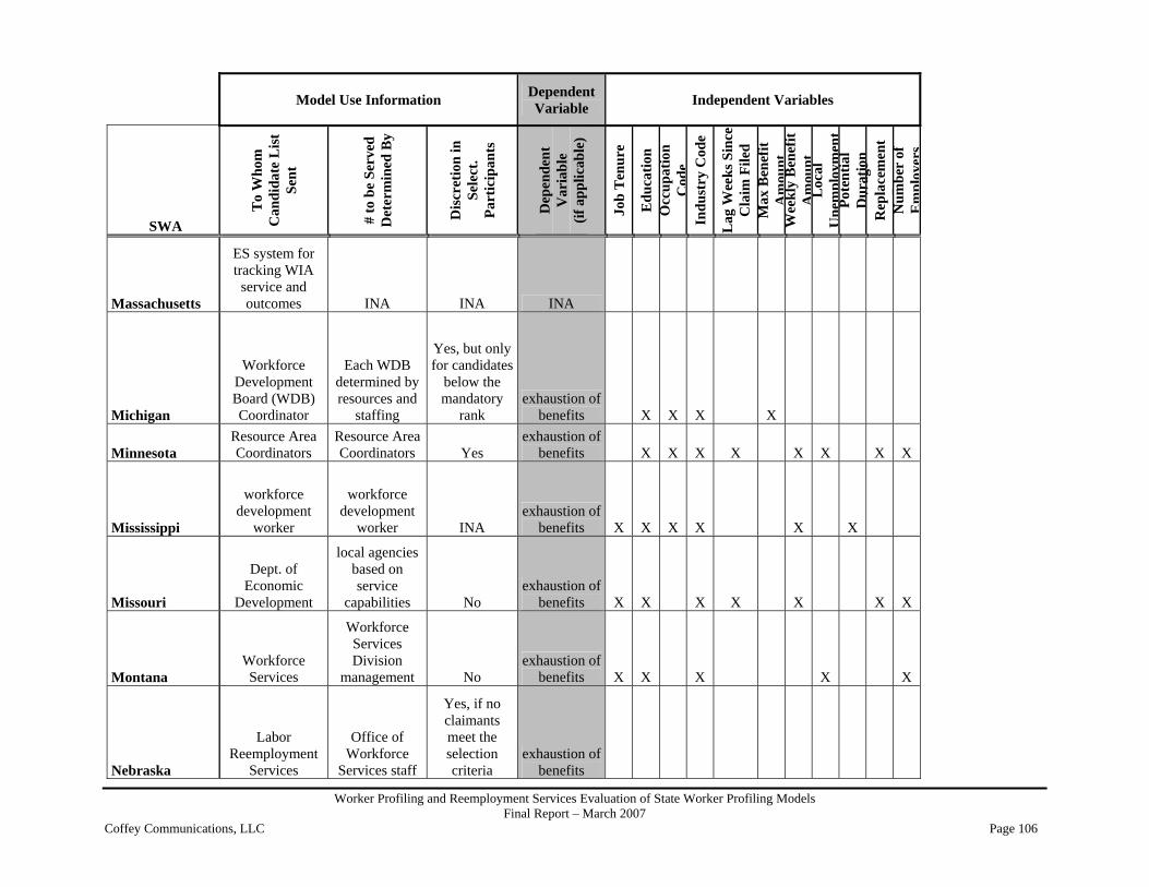
Worker Profiling and Reemployment Services Evaluation of State Worker Profiling Models Final Report – March 2007
Coffey Communications, LLC Page 106
Model Use Information Dependent Variable Independent Variables
SWA
To
Who
m
Can
dida
te L
ist
Sent
# to
be
Serv
ed
Det
erm
ined
By
Dis
cret
ion
in
Sele
ct.
Part
icip
ants
Dep
ende
nt
Var
iabl
e
(if a
pplic
able
)
Job
Ten
ure
Edu
catio
n
Occ
upat
ion
Cod
eIn
dust
ry C
ode
Lag
Wee
ks S
ince
C
laim
File
d M
ax B
enef
it A
mou
ntW
eekl
y B
enef
it A
mou
ntL
ocal
U
nem
ploy
men
tPo
tent
ial
Dur
atio
nW
age
Rep
lace
men
t R
Num
ber
of
Em
ploy
ers
Massachusetts
ES system for tracking WIA
service and outcomes INA INA INA
Michigan
Workforce Development Board (WDB) Coordinator
Each WDB determined by resources and
staffing
Yes, but only for candidates
below the mandatory
rank exhaustion of
benefits X X X X
Minnesota Resource Area Coordinators
Resource Area Coordinators Yes
exhaustion of benefits X X X X X X X X
Mississippi
workforce development
worker
workforce development
worker INA exhaustion of
benefits X X X X X X
Missouri
Dept. of Economic
Development
local agencies based on service
capabilities No exhaustion of
benefits X X X X X X X
Montana Workforce Services
Workforce Services Division
management No exhaustion of
benefits X X X X X
Nebraska
Labor Reemployment
Services
Office of Workforce
Services staff
Yes, if no claimants meet the selection criteria
exhaustion of benefits

Worker Profiling and Reemployment Services Evaluation of State Worker Profiling Models Final Report – March 2007
Coffey Communications, LLC Page 107
Model Use Information Dependent Variable Independent Variables
SWA
To
Who
m
Can
dida
te L
ist
Sent
# to
be
Serv
ed
Det
erm
ined
By
Dis
cret
ion
in
Sele
ct.
Part
icip
ants
Dep
ende
nt
Var
iabl
e
(if a
pplic
able
)
Job
Ten
ure
Edu
catio
n
Occ
upat
ion
Cod
eIn
dust
ry C
ode
Lag
Wee
ks S
ince
C
laim
File
d M
ax B
enef
it A
mou
ntW
eekl
y B
enef
it A
mou
ntL
ocal
U
nem
ploy
men
tPo
tent
ial
Dur
atio
nW
age
Rep
lace
men
t R
Num
ber
of
Em
ploy
ers
Nevada JobConnect
Office
State policy sets minimum
for JobConnect No exhaustion of
benefits x X X X X
New Hampshire local office managers
local office manager based
on staff workload
No, only veterans
programs are allowed to pick their veterans
exhaustion of benefits X X X
New Jersey Workforce New Jersey (WNJ)
local WNJ manager No
exhaustion of benefits X X X
New Mexico OWS/One-Stop
OWS/One- Stop
determined by capacity
Yes, if candidates
are seasonal workers
exhaustion/ duration of
benefits X X X
New York
All ES/WIA partner staff accessing the
One-Stop Operating Sys.
local Division of
Employment Svcs. No
exhaustion/ duration of
benefits X X X X
North Carolina local office local office managers No
exhaustion of benefits X X X X
North Dakota local One-Stop
centers local One-Stop
Centers No exhaustion of
benefits X X X

Worker Profiling and Reemployment Services Evaluation of State Worker Profiling Models Final Report – March 2007
Coffey Communications, LLC Page 108
Model Use Information Dependent Variable Independent Variables
SWA
To
Who
m
Can
dida
te L
ist
Sent
# to
be
Serv
ed
Det
erm
ined
By
Dis
cret
ion
in
Sele
ct.
Part
icip
ants
Dep
ende
nt
Var
iabl
e
(if a
pplic
able
)
Job
Ten
ure
Edu
catio
n
Occ
upat
ion
Cod
eIn
dust
ry C
ode
Lag
Wee
ks S
ince
C
laim
File
d M
ax B
enef
it A
mou
ntW
eekl
y B
enef
it A
mou
ntL
ocal
U
nem
ploy
men
tPo
tent
ial
Dur
atio
nW
age
Rep
lace
men
t R
Num
ber
of
Em
ploy
ers
Ohio State Merit Staff
district coordinators
based on One- Stop's capacity
No, unless returned to work or an exemption
applies INA
Oklahoma local offices
Profiling Coordinator in
each local office No
exhaustion of benefits
Oregon
Local business and employment services offices
Local business and
employment services offices
If number of mandatory candidates
does not fill capacity,
others can be served
exhaustion of benefits X X X X X
Pennsylvania local CareerLink
offices
local workforce
development offices
No, unless a candidate has been exempt
exhaustion of benefits X X X X X
Puerto Rico local offices
local office managers based on personnel available INA
duration of benefits

Worker Profiling and Reemployment Services Evaluation of State Worker Profiling Models Final Report – March 2007
Coffey Communications, LLC Page 109
Model Use Information Dependent Variable Independent Variables
SWA
To
Who
m
Can
dida
te L
ist
Sent
# to
be
Serv
ed
Det
erm
ined
By
Dis
cret
ion
in
Sele
ct.
Part
icip
ants
Dep
ende
nt
Var
iabl
e
(if a
pplic
able
)
Job
Ten
ure
Edu
catio
n
Occ
upat
ion
Cod
eIn
dust
ry C
ode
Lag
Wee
ks S
ince
C
laim
File
d M
ax B
enef
it A
mou
ntW
eekl
y B
enef
it A
mou
ntL
ocal
U
nem
ploy
men
tPo
tent
ial
Dur
atio
nW
age
Rep
lace
men
t R
Num
ber
of
Em
ploy
ers
Rhode Island
One- Stop offices which
profile
local office managers and staff based on
capacity
Yes, if seasonal
workers or wages are not comparable
with existing job openings
exhaustion of benefits
South Carolina local offices INA No exhaustion of
benefits X X X X X X X
South Dakota
workforce development
worker local office No exhaustion of
benefits X X X X X X X X
Tennessee local office Job
Service
coordinated between Job Service and
Field operations based on capacity No
exhaustion of benefits X X X X X
Texas
Local Workforce Development
Boards
each Board based on Capacity No
exhaustion of benefits X X X X X X X X
Utah
workforce development
worker UI director No exhaustion of
benefits X X X X X
Vermont Job Service
Offices Job Service
District office No exhaustion of
benefits X X X X X X X

Worker Profiling and Reemployment Services Evaluation of State Worker Profiling Models Final Report – March 2007
Coffey Communications, LLC Page 110
Model Use Information Dependent Variable Independent Variables
SWA
To
Who
m
Can
dida
te L
ist
Sent
# to
be
Serv
ed
Det
erm
ined
By
Dis
cret
ion
in
Sele
ct.
Part
icip
ants
Dep
ende
nt
Var
iabl
e
(if a
pplic
able
)
Job
Ten
ure
Edu
catio
n
Occ
upat
ion
Cod
eIn
dust
ry C
ode
Lag
Wee
ks S
ince
C
laim
File
d M
ax B
enef
it A
mou
ntW
eekl
y B
enef
it A
mou
ntL
ocal
U
nem
ploy
men
tPo
tent
ial
Dur
atio
nW
age
Rep
lace
men
t R
Num
ber
of
Em
ploy
ers
Virgin Islands Reemployment
Services UI director
Yes, for candidates
with unresolved
issues
exhaustion of benefits and duration of
benefits X X X X
Virginia
local and central offices via mainframe
local office based on capacity
Yes, for candidates
that will drop off the list if not selected
exhaustion of benefits X X X X X
Washington WorkSource
Offices WorkSource
office
Yes, for similar or
same service exhaustion of
benefits
West Virginia INA
Job Service local office
staff No exhaustion of
benefits X X X X X X
Wisconsin none
local office based on capacity No
exhaustion of benefits X X X X X
Wyoming
profiling coordinator at
the state claims center
profiling coordinator No
exhaustion of benefits X X X X X X X
1 - Individuals who are exempt from work search requirements are not eligible for referral to WPRS services 2 - Claimants with delayed payments or earnings during the first week of benefits are not eligible for referral to WPRS services
INA - Information Not Available

Worker Profiling and Reemployment Services Evaluation of State Worker Profiling Models Final Report – March 2007
Coffey Communications, LLC Page 111
APPENDIX C
REPORTS FOR 53 SWAS AND
DECILE TABLES FOR 28 SWAS

Worker Profiling and Reemployment Services Evaluation of State Worker Profiling Models Final Report – March 2007
Coffey Communications, LLC Page 112
ANALYSIS OF ALABAMA PROFILING MODEL
Introduction:
Alabama uses a statistical model, of which the functional form is logistic, to determine a claimant’s
Worker Profiling and Reemployment Services (WPRS) profiling score. This model is run weekly against
the claimant first payment file and the list of eligible candidates, ranked by probability of exhaustion, is
produced at that time and sent to career centers via the Alabama Job Link System. The number of
candidates to be selected to receive services is based on the size of the career center with claimants to be
served being prioritized by their probability of exhaustion. The career centers have no discretion in the
selection of candidates and must service each succeeding candidate starting with those claimants with the
highest probability of exhaustion.
The model is revised approximately every three years with a substantial revision being undertaken
approximately six years ago. During this revision, a continuous variable was incorporated into the model
which is reflected in all future model revisions. Prior to revising the current model, its accuracy is
evaluated to ascertain what modifications are needed. Those claimants who are required to perform work
search are included in the sample for profiling with the most recent sample consisting of 23,561
claimants. The original model had 20,000 claimants in the sample but was reduced to 7,000 due to
computer capacity.
Data Collection Process:
Initial claims are filed by telephone only. The occupational code is determined by the initial claims taker
using the Standard Occupational Classification (SOC) system, and no verification is performed to
ascertain the accuracy of the information provided by the claimant. The primary employer classification
is determined by a review of the claimant’s wage records. Individuals who are exempt from work search
requirements in Alabama are not eligible for referral to WPRS services.

Worker Profiling and Reemployment Services Evaluation of State Worker Profiling Models Final Report – March 2007
Coffey Communications, LLC Page 113
Selection/Referral Process:
Candidates selected to be referred to services are based on running the weekly WPRS model against the
first payment file. The list of candidates is produced at that time and is sent to Career Centers using the
Alabama Job Link System. The number to be selected for service is based on the size of the Career
Center. Claimants are listed by probability of exhaustion and they cannot be skipped. Career Center staff
members have no control over the listing.
Profiling Model Structure:
The dependent variable used in the WPRS model is benefit exhaustion, defined as maximum benefits
paid, receiving 26 weekly benefit payments, or zero dollars of benefit entitlement remaining. The
selected independent variables were based on a study of variable options by the Employment and
Training Administration national and regional staff. The result of this study was a list of variables which
were determined to have a reasonable probability of statistical significance. Alabama’s variables were
selected from those recommended, and include the following:
• Tenure
• Weekly Benefit Amount
• Education
• Industry
• Occupation
Note, there are four occupation variables used in Alabama’s profiling model – high rate of exhaustion
(OCC4), moderately high rate of exhaustion (OCC3), low rate of exhaustion (OCC2), and midrange rate
of exhaustion (OCC1). Occupation codes are determined after exhaustion rates for each occupation are
calculated and listed in descending order by exhaustion rate. This list is then divided into the four
categories with those benefit recipients in occupations with high rates of exhaustion being assigned to
OCC4 with a coefficient of 0.5657.

Worker Profiling and Reemployment Services Evaluation of State Worker Profiling Models Final Report – March 2007
Coffey Communications, LLC Page 114
Alabama’s model has at least one continuous variable (either Weekly Benefit Amount or Tenure) to
prevent a large number of ties. Claimants with missing data are assigned the mid-range value for
categorical variables such as OCC1 for missing occupation data. Alabama does not eliminate missing
and/or incomplete records since elimination of the records would, in theory, reduce the accuracy of their
model.
Profiling Model Performance:
Alabama did not provide a dataset for data analysis and/or model revision; therefore, we were unable to
gauge the performance of its current model.

Worker Profiling and Reemployment Services Evaluation of State Worker Profiling Models Final Report – March 2007
Coffey Communications, LLC Page 115
ANALYSIS OF ALASKA PROFILING MODEL
Introduction:
Alaska uses a statistical model, of which the functional form is logistic regression, to determine a
claimant’s Worker Profiling and Reemployment Services (WPRS) profiling score. The model is run
weekly against the claimant first payment file, and a listing of those determined eligible is displayed in
the Unemployment Insurance (UI) mainframe system (DB2). The ES recently converted to a new on-line
system and negotiations are currently underway with the service provider to determine the referral to
reemployment services process. This list ranks candidates in order from highest probability of exhaustion
to lowest.
The model is reviewed annually to ascertain if it should be updated and/or revised. It was most recently
updated in January 2006, and revised in January 2005. During the January 2005 revision, the variable
comparing the date of first payment with day the claim began was added to the model and the variable for
the exhaustion rate for the local offices was eliminated. Over 107,000 benefit recipients were used as the
sample in the most recent revision.
Data Collection Process:
Initial claims are filed by telephone (92%) and internet (8%). Claimant characteristics necessary to
determine an individual’s eligibility for WPRS are obtained during the initial filing process. The
accuracy of data is checked during random audits conducted as part of the Benefit Accuracy
Measurement (BAM) Program. In claims filed telephonically, the claimant’s occupational code is
assigned by the initial claims taker. In claims filed on the Internet, the occupational code is self-selected
by the claimant using a drop-down menu. The UI database uses a crosswalk to the Job Service system to
convert the occupational code from Dictionary of Occupational Titles (DOT) system classification to
Standard Occupational Classification (SOC) system classification. However, it is important to note that
the occupational code is not used in the WPRS model. The industry code is assigned based on the
claimant’s last employer and is verified through a review of the UI wage record system. The following
individuals are not eligible for WPRS services:
• Claimants who received orientation services in the previous year
• Claimants who reside outside of Alaska; or who reside in rural Alaskan areas not serviced by a
Job Service office

Worker Profiling and Reemployment Services Evaluation of State Worker Profiling Models Final Report – March 2007
Coffey Communications, LLC Page 116
• Claimants who have separated from their last employment for reasons other than a lack of work
• Claimants who are not required to be fully registered for work with the Alaska Labor Exchange
Service
Selection/Referral Process:
The WPRS model is run against the claimant first payment file, and a listing of eligible candidates is
produced at that time. The list is arrayed with those individuals most likely to exhaust listed first with the
least likely last; it is then displayed in the UI mainframe system (DB2). At the current time, negotiations
are ongoing to determine the referral process to be used for selected individuals to receive services. The
Employment Service unit of the Agency determines the number of candidates to be served based upon
staff and facility capacity. Selection for services begins with those with the greatest likelihood of
exhausting benefits and the highest probability score and continues in descending order until the
limitations of the service provider have been met.
Profiling Model Structure:
The WPRS profiling model employed by Alaska utilizes a statistical model, of which the functional form
is logistic, to estimate benefit exhaustion. The dependent variable used in the model equation is benefit
exhaustion, which is defined as the receipt of the maximum benefit amount. Alaska uses a wide array of
independent variables, which are as follows:
• Quarter of claim beginning
• Education
• Number of employers in the base period with wage
• Number of dependents times eligible weeks of the claim divided by weekly benefits
• Hiring index based on the industry and geographic region of the state
• Minimum unemployment weighted index based on the geographic region of the state and three
years of history
• Weekly benefits divided by the average base period wages
• Reason for separation from employment
• Difference in days between the first pay date and the claim begin date
• History of prior years UI claims
• Duration of claim

Worker Profiling and Reemployment Services Evaluation of State Worker Profiling Models Final Report – March 2007
Coffey Communications, LLC Page 117
• Experience measured by the number of days worked for the previous employer
Profiling Model Performance: Alaska did not provide a dataset for data analysis and/or model revision; therefore, we were unable to
gauge the performance of its current model.
Worker Profiling and Reemployment Services Evaluation of State Worker Profiling Models Final Report – March 2007
Coffey Communications, LLC Page 118
ANALYSIS OF ARIZONA PROFILING MODEL
Introduction:
Arizona uses a statistical model, of which the functional form is logistic, to determine a claimant’s
Worker Profiling and Reemployment Services (WPRS) profiling score. The model is run daily against the
claimant first payment file; however, the list of eligible candidates is not run until an orientation roster
request is submitted by an orientation provider. Selection for participation in orientation is automated by
a ranking score with those most likely to exhaust Unemployment Insurance (UI) benefits being ranked
higher.
Currently, the model is updated every two to three years with the last update occurring in July 2003. At
that time, the original model was replaced with a WPRS intranet application developed by Scott Gibbons
of the U. S. Department of Labor. The original model had not been updated since its inception in 1994.
Currently, there is no policy in place for Arizona that addresses the frequency of model revisions.
However, the Research Administration of the Arizona Department of Economic Security and the
Employment Administration MIS section will be working together in the future to establish regular
reviews of the ability of the model to predict exhaustion.
Data Collection Process:
Initial claims are filed in-person, by telephone and via the Internet. Claimant characteristics necessary to
determine an individual’s eligibility for WPRS services are captured at the time of the initial claim filing.
The claimant’s social security number is verified for accuracy. The occupational code is not captured or
used in the model. North American Industry Classification System (NAICS) codes are used as the
industry classification system and are assigned based on the applicant’s last employer. Individuals not
eligible for referral to WPRS services include:
• Union members on the out-of-work list
• Claimants who reside more than 25 miles from available services
• Seasonal workers
• Workers who are attached to their last employer

Worker Profiling and Reemployment Services Evaluation of State Worker Profiling Models Final Report – March 2007
Coffey Communications, LLC Page 119
Selection/Referral Process:
Selection for participation in WPRS services is automated using a ranking score. Selection from the pool
is made when an orientation provider enters a request for a roster of candidates. Program Managers
determine the number of claimants to be scheduled for each of the four service districts based on the
availability of staff to provide services. Local areas cannot select candidates. Selection is based upon the
number requested and the number available in the pool for the orientation provider.
Profiling Model Structure: The WPRS profiling model employed by Arizona utilizes a statistical model, of which the functional
form is logistic, to estimate benefit exhaustion. The dependent variable used in the equation is benefit
exhaustion, defined as the payment of the maximum benefit amount. The independent variables used in
the model for Arizona include:
• Job Tenure
• Delay in Filing
• County of Residence
• Education
• NAICS Classification
• Month in Which the Initial Claim is Filed
• Wage Replacement Rate
• Maximum Benefit Amount
Profiling Model Performance: Arizona provided the model structure and dataset for data analysis but did not provide useable data for
education; therefore, we did not conduct an extended analysis for Arizona. We did calculate a decile
table for Arizona with a correction for endogeneity. It is shown below.
prorigdec mean se(mean)
1 0.350 0.0062 0.330 0.0063 0.348 0.0064 0.346 0.006

Worker Profiling and Reemployment Services Evaluation of State Worker Profiling Models Final Report – March 2007
Coffey Communications, LLC Page 120
5 0.341 0.0066 0.375 0.0067 0.373 0.0068 0.400 0.0069 0.418 0.007
10 0.508 0.007 Total 0.379 0.002
We also calculated the metric that shows the effectiveness of Arizona’s profiling score. It is shown
below.
SWA Profiling score
Control for endogeneity?
Exhaustion rate for the
state
Number of individuals
with the highest profiling score
Exhaustion rate for
individuals with high profiling scores
Metric Variance of the Metric
Standard Error of
the metric
Arizona original score Y 37.9 21,502 42.8 0.079 1.153 0.007
The metric has a value of 0.079 and a standard error of 0.007. The metric is useful because it is
significantly greater than 0 and provides a basis for comparison with other profiling models.

Worker Profiling and Reemployment Services Evaluation of State Worker Profiling Models Final Report – March 2007
Coffey Communications, LLC Page 121
ANALYSIS OF ARKANSAS PROFILING MODEL
Introduction:
Arkansas uses a statistical model, of which the functional form is linear (multiple regression), to
determine a claimant’s Worker Profiling and Reemployment Services (WPRS) profiling score. The model
is run weekly against the claimant first payment records, and the list of WPRS eligible claimants is sent
electronically to the Local Office Job Search Workshop Coordinators. This list ranks candidates in order
from highest probability of exhaustion to lowest, and those with higher rankings are to receive services
first. The Coordinators determine the number of eligible candidates to be served and cannot skip down
the list. The model has not been revised and/or updated since its implementation.
Prior to implementation, a study was conducted on a sample of 10 percent of 1994 fiscal-year benefit
recipients. The model predicted 2,180 claimants would exhaust out of a total sample of 5,154. In reality,
50.9 percent (1,110) did actually exhaust their benefits. The model also predicted that 2,974 would not
exhaust, and in reality, 2,134 actually did not exhaust. Therefore, the model predicted about 63 percent of
the claimants’ exhaustion/non-exhaustion experience correctly.
Arkansas is contemplating an update of the model which would allow occupational codes to be obtained
from ES O*Net codes and then translated to Standard Occupational Classification (SOC) system codes.
This update would also allow employment change factors to be used and would switch to the North
American Industry Classification System (NAICS) instead of Standard Industrial Classification (SIC)
Codes.
Data Collection Process:
Initial claims are filed in-person, by mail, and through self-service computers in the local offices. In order
to determine an individual’s eligibility for WPRS, initial claims are processed using a combination of
automated records and information obtained from the claimants themselves. Wages, industrial code,

Worker Profiling and Reemployment Services Evaluation of State Worker Profiling Models Final Report – March 2007
Coffey Communications, LLC Page 122
benefit rate and benefit duration are obtained from the agency’s automated records. The occupational
classification is assigned by the initial claims taker. There are no further checks on the accuracy of
information provided by the claimant. Individuals not eligible for referral to services through WPRS
include:
1 Interstate claimants
2 Shared work claimants
3 Claimants who are work-search exempt because they are still job attached (working part-time for
the employer) or expect to be recalled within 10 weeks
4 Claimants who have a union attachment with an expectation of recall
5 Claimants in training
Selection/Referral Process:
Claimants eligible for services through WPRS are selected when they receive their first payment. They
are ranked in order by workforce area, and claimants with the highest probabilities of exhausting benefits
are ranked first, second, etc. The list is sent electronically each week to the Local Office Workshop
Coordinators. Simultaneously, claimants who are selected are sent a notice informing them that they have
been profiled. The number of clients who attend Job Search Workshops and the primary service provided
to profiled candidates are determined by the availability of Job Search Workshop Coordinators and of
workshop seating space in the various communities throughout the state. The Coordinators select from
the list on a top-down basis. Individuals are removed from the list after seven weeks.
Profiling Model Structure:
The WPRS profiling model employed by Arkansas uses a statistical model, of which the functional form
is linear (multiple regression), to estimate the probability of exhaustion. The dependent variable used in
the model is the estimated probability of exhaustion score limited to a range between zero and one.
Independent variables used in the model are:

Worker Profiling and Reemployment Services Evaluation of State Worker Profiling Models Final Report – March 2007
Coffey Communications, LLC Page 123
• Potential Duration
• Ratio of Claimant’s WBA to the State Allowable MBA
• Industry
• Occupation
• Education
• Job Preparation/Appropriateness
• Residence in Specific Workforce Areas
In selecting the variables listed above, a maximum likelihood estimator was used to evaluate each
available variable, and from this, a multiple regression equation was derived using the appropriate
variables.
Profiling Model Performance:
Our first step was to try to replicate the given score using the data and coefficients provided. From the
given data, we identified the variables used in the model, including potential duration of receipt of
unemployment benefits, ratio of weekly benefit allowance to maximum benefit allowance, workforce
delivery area code, industry code, actual change and percentage change in the industry, occupation code,
level of education, and a binary variable for the claim taker’s indication of insufficient job preparation.
No check for endogeneity was possible because there was no record of referral to reemployment services.
To show the performance of the original profiling score, we ordered individuals into deciles and
calculated the exhaustion rate for each decile along with the standard error. This decile table is how we
demonstrate the effectiveness of each model. The decile means are calculated by dividing the percentage
of recipients that exhaust benefits for a given decile by 100. For example, in the first decile our mean is
0.378, which indicates that approximately 38 percent of benefit recipients in this decile exhausted
benefits.

Worker Profiling and Reemployment Services Evaluation of State Worker Profiling Models Final Report – March 2007
Coffey Communications, LLC Page 124
Decile Mean Standard Error (Mean) 1 .378 .0066832 .462 .00685143 .466 .00689264 .483 .00688915 .471 .00687146 .49 .00689947 .495 .00689458 .522 .00688349 .576 .006809610 .646 .00659 Total .499 .0021791
Using the provided dataset, we continued our analysis of the Arkansas profiling model by creating three
models – an updated, a revised, and a Tobit model. For each of the models, new profiling scores were
created, ranked, and divided into deciles. The table below shows the decile gradient for each of our
models (detailing the mean for each decile) and includes the decile gradient for the original model for
reference. From the table, we see that there was an improvement between the original and updated
models and further improvement in the decile gradient between the updated and revised models.
Decile Original score Updated score Revised score Tobit score 1 .378 .345 .326 .338 2 .462 .421 .413 .415 3 .466 .455 .425 .422 4 .483 .474 .47 .458 5 .471 .486 .476 .483 6 .49 .491 .503 .509 7 .495 .502 .534 .524 8 .522 .535 .551 .543 9 .576 .588 .606 .606 10 .646 .694 .685 .691 Total .499 .499 .499 .499
While there was improvement between the original and updated and revised models, there was no
significant improvement between the revised and the Tobit models. As such, the revised model appears

Worker Profiling and Reemployment Services Evaluation of State Worker Profiling Models Final Report – March 2007
Coffey Communications, LLC Page 125
to be the best model using the data available (see Appendix D for information on revised model).
Additionally, we tested the performance of each model using the metric described below:
Percent exhausted of the top 49.9% of individuals in the score.
We used 49.9 percent because the exhaustion rate for benefit recipients in the dataset provided by
Arkansas was 49.9 percent. This metric will vary from about 49.9 percent, for a score that is a random
draw, to 100 percent for a score that is a perfect predictor of exhaustion. The scores for the four models
are as follows:
Score % exhausted of those with the top 49.9% of score Standard error of the score Original 54.64 0.30716 Updated 56.24 0.30606 Revised 57.62 0.30486 Tobit 57.51 0.30497 In the below metric, “Exhaustion” is the percentage of all benefit recipients in our sample that exhaust
benefits. Here we use 49.9 percent for “Exhaustion” because the exhaustion rate for all benefit recipients
for Arkansas was 49.9 percent. “Pr[Exh]” in our metric is determined by the model with the highest
percentage of benefit exhaustees with profiling scores falling in the top X percent of the sample, where X
percent is determined by the exhaustion rate for all benefit recipients in the sample. For Arkansas,
“Pr[Exh]” is represented by the revised model with a score of 57.62 percent for benefit recipients that
exhaust benefits with scores falling in the top 49.9 percent.
100 – Pr[Exh] Metric: 1 – 100 – Exhaustion
We used the numbers above to calculate a score of 0.095 for the original score and 0.154 for the revised
model score.
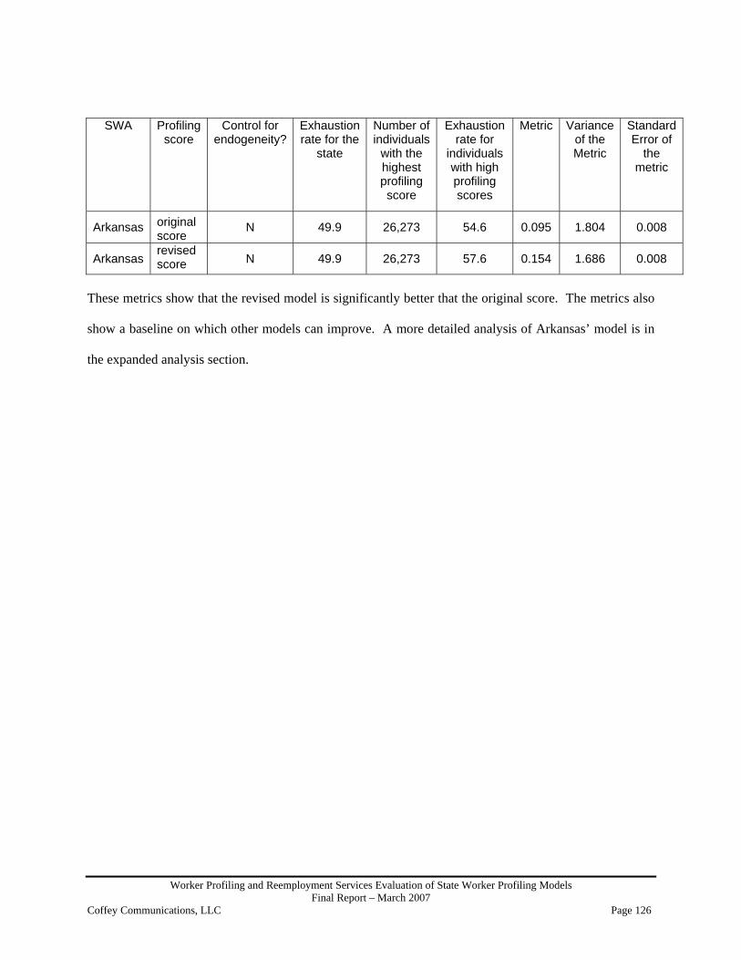
Worker Profiling and Reemployment Services Evaluation of State Worker Profiling Models Final Report – March 2007
Coffey Communications, LLC Page 126
SWA Profiling score
Control for endogeneity?
Exhaustion rate for the
state
Number of individuals
with the highest profiling score
Exhaustion rate for
individuals with high profiling scores
Metric Variance of the Metric
Standard Error of
the metric
Arkansas original score
N 49.9 26,273 54.6 0.095 1.804 0.008
Arkansas revised score N 49.9 26,273 57.6 0.154 1.686 0.008
These metrics show that the revised model is significantly better that the original score. The metrics also
show a baseline on which other models can improve. A more detailed analysis of Arkansas’ model is in
the expanded analysis section.

Worker Profiling and Reemployment Services Evaluation of State Worker Profiling Models Final Report – March 2007
Coffey Communications, LLC Page 127
ANALYSIS OF CALIFORNIA PROFILING MODEL
Introduction:
California uses both a characteristic screen and a statistical model, of which the functional form is
logistic, to determine a claimant’s Worker Profiling and Reemployment Services (WPRS) profiling score.
The model is run weekly against the claimant first payment records with a list of WPRS eligible claimants
being sent electronically to the Employment Service Scheduling System. This list ranks candidates in
order from highest probability of exhaustion to lowest with those with higher rankings scheduled to
receive services first.
The Field Office Manager or Initial Assistance Workshop (IAW) Leader determines the number of
claimants to be served based on available staffing and office accommodations. The IAW is less than a
day and consists of a discussion of why claimants are selected, Unemployment Insurance eligibility, labor
market information, and orientation to other reemployment services. Local offices cannot “skip down the
rank” in selecting candidates for services. The candidates must be served in order of their probability of
exhaustion.
Currently, there is no system in place to determine when the model is to be updated. The model was last
updated on December 31, 2001 and has never been revised.
Data Collection Process: Initial claims are filed by telephone (60 pecent), by mail (5 percent), and via the internet (35 percent).
Characteristic data for claimants is captured at the time initial claims are filed; currently there is no check
for accuracy of data. If the claim is taken by telephone, the initial claims taker assigns the claimant’s
occupational code. If the claim is filed by mail, the occupation code is self-reported. For those filing via
the Internet, there is currently a drop down menu in place for occupation code selection. The
occupational code is determined jointly using the Dictionary of Occupational Titles (DOT) system and the
Standard Occupational Classification (SOC) System. The claimant’s primary employer is determined by
a review of the claimant’s wage history and UI Wage records. Individuals not eligible for referral to
WPRS services include seasonal workers and active union members.

Worker Profiling and Reemployment Services Evaluation of State Worker Profiling Models Final Report – March 2007
Coffey Communications, LLC Page 128
Selection/Referral Process: A listing ranks the candidates in order from the highest probability of exhaustion to the lowest, and those
with higher rankings are scheduled to receive services first. The Field Office Manager or IAW Workshop
Leader determines the number of claimants to be served based on available staffing and office
accommodations. Local offices cannot “skip down the rank” in selecting candidates for services. The
candidates must be served in order of their probability of exhaustion.
Profiling Model Structure:
The WPRS profiling model employed by California utilizes both a characteristic screen and statistical
model, of which the functional form is logistic, to estimate benefit exhaustion and likelihood of long-term
unemployment. The characteristic screen is used to determine whether or not a claimant will be recalled
to employment or if the claimant is a union member.
The dependent variables used in the model are exhaustion of benefits and long-term unemployment,
defined, respectively, as the payment of the maximum benefit amount and 24 weeks or more of benefits
paid within 12 months after filing. The independent variables used are:
• Education
• Industry
• Occupation
• Job Tenure
• County and/or Workforce Area
As mentioned, California pre-screens applicants to determine whether or not they will be recalled prior to
first benefit payment and whether or not they are a union member. This pre-screen takes place via the
characteristic screen.
Profiling Model Performance: California did not provide a dataset for data analysis and/or model revision; therefore, we were unable to
gauge the performance of its current model.

Worker Profiling and Reemployment Services Evaluation of State Worker Profiling Models Final Report – March 2007
Coffey Communications, LLC Page 129
ANALYSIS OF COLORADO PROFILING MODEL
Introduction: Colorado uses a statistical model, of which the functional form is logistic, to determine a claimant’s
Worker Profiling and Reemployment Services (WPRS) profiling score. The model is run weekly against
the claimant first payment file, and a list of eligible candidates is generated at that time. This list, ordered
from highest probability score to lowest, is then sent by file transfer to workforce centers who determine
how many profiled candidates will be served. A center may exempt a candidate for various reasons, such
as the candidate being a previous client of the center. It has been more than three years since the model
was revised, and it has not been updated since implementation. The original sample size, when the model
was first estimated, was approximately 40,000.
Data Collection Process:
Initial claims are filed by telephone (80 percent) and Internet (20 percent). All claimant characteristic
data necessary to determine WPRS services eligibility are captured during the initial telephone or Internet
filing. If a filing is done telephonically, the initial claims taker will determine and assign the claimant’s
occupational code. If done via internet, the occupational code is self-selected by the claimant. Both filing
methods use the Standard Occupational Classification (SOC) system. A review of wage records is used
to determine the appropriate industry code. Persons who are job attached, whose first payments are more
that five weeks from filing of the initial claim, and those who are hired through union halls are not
eligible for referral to WPRS services.
Selection/referral Process:
The model is run weekly against the claimant first payment file, and a list of eligible candidates is
generated at that time. The list, ordered from highest probability of exhaustion score to the lowest, is then
sent by file transfer to workforce centers who determine how many candidates will be served. A center
may exempt a candidate for various rerasons, i.e. the candidate was a previous client of the center.
Profiling Model Structure: The WPRS profiling model employed by Colorado utilizes a statistical model, of which the functional
form is logistic, to estimate benefit exhaustion. The dependent variable used in the model equation is

Worker Profiling and Reemployment Services Evaluation of State Worker Profiling Models Final Report – March 2007
Coffey Communications, LLC Page 130
benefit duration defined as maximum benefits paid. Colorado did not provide any information on the
independent variables used in their model.
Profiling Model Performance:
Colorado did not provide a dataset for data analysis and/or model revision; therefore, we were unable to
gauge the performance of Colorado’s current model.

Worker Profiling and Reemployment Services Evaluation of State Worker Profiling Models Final Report – March 2007
Coffey Communications, LLC Page 131
ANALYSIS OF CONNECTICUT PROFILING MODEL
Introduction:
Connecticut uses a statistical neural network model to determine a claimant’s eligibility for referral to
Worker Profiling and Reemployment Services (WPRS). The model is run weekly against the claimant
first payment records, and a listing of WPRS eligible claimants is sent to the Connecticut Department of
Labor (DOL) staff via computer network. The model was last revised in July 2004. The latest revision
converted the model form to that of a neural networking model.
Data Collection Process:
Initial claims are filed by telephone (91.1 percent) and Internet (8.9 percent). Claimant characteristics are
captured at the time the initial claim is filed, and there are no further checks for accuracy. When a claim
is taken by telephone, the initial claims taker assigns the claimant’s occupational code using the O*NET
classification system and when done online, the occupational code is self-selected by the claimant. The
NAICS of the claimant’s primary employer is assigned from wage records even though industry is not
used as a variable in the model. The following claimants are not eligible for referral to WPRS services:
• Union workers who get employment through hiring halls
• Job attached workers
Selection/Referral Process: The list of profiled candidates is produced at the same time the weekly WPRS model is run, and the list is
then sent to Connecticut DOL Staff via computer network. Claimants with the highest probability of
exhaustion are selected first for services and the Connecticut DOL Job Center Directors determine how
many profiling candidates will be served per office with some input from central office staff.
Profiling Model Structure: The Connecticut WPRS profiling model utilizes a neural network model to estimate benefit exhaustion.
The dependent variable in the model equation is benefit exhaustion. The independent variables are as
follows:
• Education

Worker Profiling and Reemployment Services Evaluation of State Worker Profiling Models Final Report – March 2007
Coffey Communications, LLC Page 132
• Tenure
• Occupation
• Effective Date of Claim
• Workforce Area
• Veteran Status
• Weekly Benefit Rate
• Prior Claims
• Prior Exhaustion
Profiling Model Performance:
With their survey, Connecticut provided a dataset and the model structure. However, the data did not
indicate whether individuals exhausted benefits. Therefore, we were not able to calculate a metric or
conduct an expanded analysis of the model.

Worker Profiling and Reemployment Services Evaluation of State Worker Profiling Models Final Report – March 2007
Coffey Communications, LLC Page 133
ANALYSIS OF DELAWARE PROFILING MODEL
Introduction: Delaware uses a characteristic screen to determine a claimant’s eligibility for Worker Profiling and
Reemployment Services (WPRS). The model is run weekly against the claimant first payment records
with a list of WPRS eligible claimants being sent to the Division of Employment and Training. All
individuals who meet WPRS selection criteria are listed, notified, and required to participate in the WPRS
program.
The model has never been updated and/or revised since the inception of WPRS. Delaware evaluated the
variables used for WPRS against the actual claims filed to determine the need for possible modification.
The SWA examined the characteristics of claimants that actually filed over a period of time and examined
what participation would be if the current variables were modified.
Data Collection Process:
Initial claims are filed by mail and in-person. Internet claim filing is currently in development. With the
exception of the occupational code, information necessary to make a profiling referral is captured at the
time the initial claim is filed. The occupational code will be selected by the claimant from a drop-down
box when a claimant completes reemployment registration information online. There is no further check
on the accuracy of the claimant’s selection. The last employer is also selected from the reemployment
application, and that employer’s North American Industry Classification System (NAICS) code is
captured from the UI employer file. Individuals not eligible for referral to WPRS services include:
• Claimants with a return-to-work date
• Claimants who belong to a union and obtain their work through a union hiring hall
• Claimants who have received more than five weeks of benefit payments
Selection/Referral Process:
All claimants eligible for WPRS are listed and sent to the Division of Employment administrative staff.
Subsequently, all claimants are notified and required to participate in WPRS. There are no feedback
loops in place.
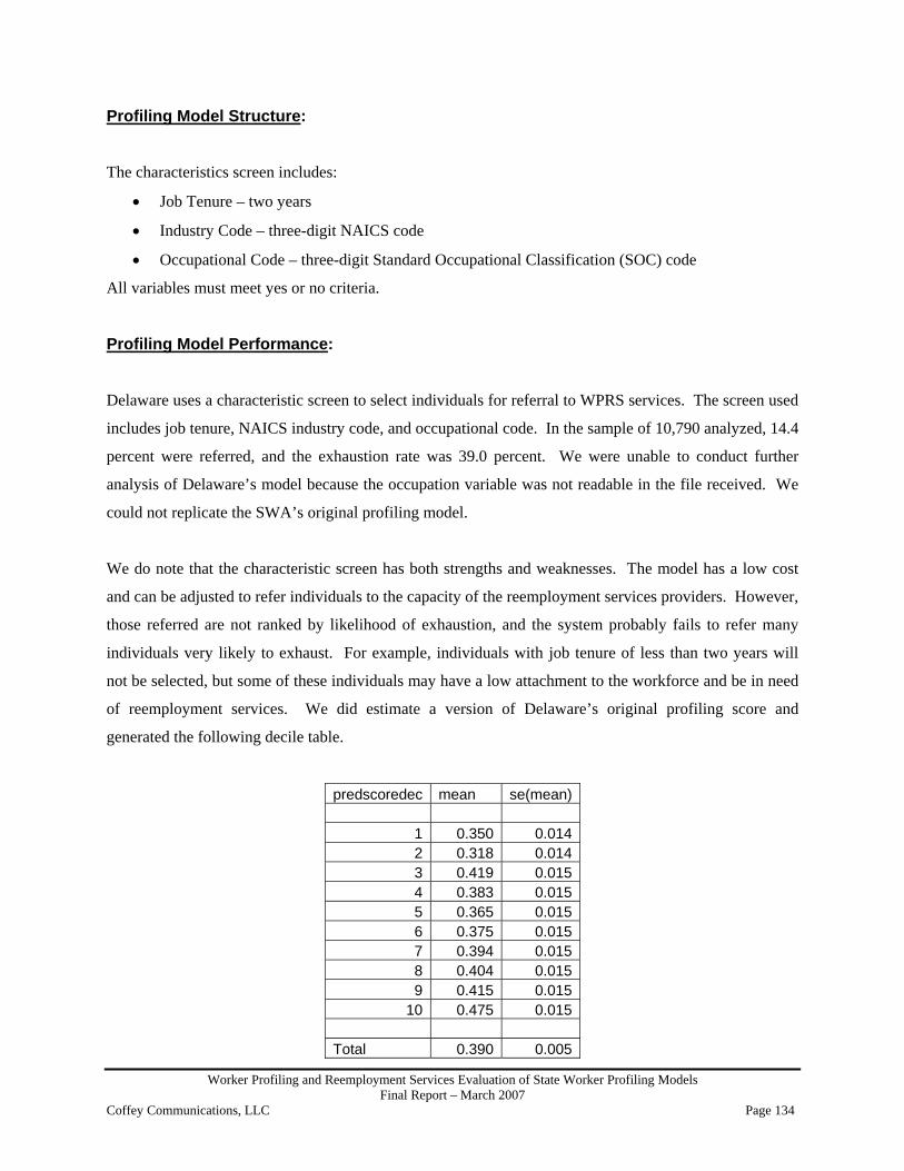
Worker Profiling and Reemployment Services Evaluation of State Worker Profiling Models Final Report – March 2007
Coffey Communications, LLC Page 134
Profiling Model Structure:
The characteristics screen includes:
• Job Tenure – two years
• Industry Code – three-digit NAICS code
• Occupational Code – three-digit Standard Occupational Classification (SOC) code
All variables must meet yes or no criteria.
Profiling Model Performance: Delaware uses a characteristic screen to select individuals for referral to WPRS services. The screen used
includes job tenure, NAICS industry code, and occupational code. In the sample of 10,790 analyzed, 14.4
percent were referred, and the exhaustion rate was 39.0 percent. We were unable to conduct further
analysis of Delaware’s model because the occupation variable was not readable in the file received. We
could not replicate the SWA’s original profiling model.
We do note that the characteristic screen has both strengths and weaknesses. The model has a low cost
and can be adjusted to refer individuals to the capacity of the reemployment services providers. However,
those referred are not ranked by likelihood of exhaustion, and the system probably fails to refer many
individuals very likely to exhaust. For example, individuals with job tenure of less than two years will
not be selected, but some of these individuals may have a low attachment to the workforce and be in need
of reemployment services. We did estimate a version of Delaware’s original profiling score and
generated the following decile table.
predscoredec mean se(mean)
1 0.350 0.0142 0.318 0.0143 0.419 0.0154 0.383 0.0155 0.365 0.0156 0.375 0.0157 0.394 0.0158 0.404 0.0159 0.415 0.015
10 0.475 0.015 Total 0.390 0.005

Worker Profiling and Reemployment Services Evaluation of State Worker Profiling Models Final Report – March 2007
Coffey Communications, LLC Page 135
In addition, we calculated the metric associated with this estimated score. It is shown below.
SWA Profiling score
Control for endogeneity?
Exhaustion rate for the
state
Number of individuals
with the highest profiling score
Exhaustion rate for
individuals with high profiling scores
Metric Variance of the Metric
Standard Error of
the metric
Delaware estimated score* N** 39.0 4,207 42.4 0.055 1.227 0.017
The metric has a value of 0.055 and a standard error of 0.017. The metric is useful because it is
significantly greater than 0, and provides a basis for comparison with other profiling models.

Worker Profiling and Reemployment Services Evaluation of State Worker Profiling Models Final Report – March 2007
Coffey Communications, LLC Page 136
ANALYSIS OF THE DISTRICT OF COLUMBIA PROFILING MODEL
Introduction:
The District of Columbia uses a statistical model, of which the functional form is logistic, to determine a
claimant’s Worker Profiling and Reemployment Services (WPRS) profiling score. The model is run
weekly against the claimant first payment records with a list of WPRS eligible claimants being sent
electronically via an intranet to the management staff of the One-Stops. This list ranks candidates in
order from highest probability of exhaustion to lowest, with those with higher rankings scheduled to
receive services first. One-Stop staff then determines the number of eligible claimants to be called in to
receive services. The model was updated in January 2004, and is updated every two or three years.
In October 2003, the model was revised by adding the “Filing Delay” and “Number of Employers”
variables. The coefficients were calculated using 5,000 benefit recipients. The previous model was
estimated using 4,000 recipients. During the 2003 revision, the occupational coding was changed from
Dictionary of Occupational Titles (DOT) to O*Net.
Data Collection Process:
Eighty percent of the initial claims are filed over the Internet, and the remaining 20 percent are filed in-
person. Characteristic data are captured when the initial claim is filed and the correct North American
Industry Classification System (NAICS) code is determined based on a review of wage records. When
claims are filed via the Internet, occupation codes are automatically generated based on information
provided by the claimant using O*Net criteria. When claims are filed in-person, the initial claims taker
assigns the appropriate codes. Currently, there are no checks on the accuracy of the information provided
by the claimant. Individuals not eligible for referral to services through WPRS include:
• Interstate claimants
• Transitional claimants
• Claimants involved in a labor dispute
• Claimants on temporary furlough
• Members of a union with a hiring hall
• Prior WPRS participants
• Claimants with earnings during the first week of benefits

Worker Profiling and Reemployment Services Evaluation of State Worker Profiling Models Final Report – March 2007
Coffey Communications, LLC Page 137
• Claimants with delayed payments
Profiling Model Structure:
The WPRS profiling model employed by the District of Columbia utilizes a statistical model, of which
the functional form is logistic, to estimate benefit exhaustion. The dependent variable is benefit
exhaustion, defined as the payment of the maximum benefit amount. The independent variables include:
• Unemployment Rate
• Job Tenure
• Level of Education
• Occupation Code
• Industry Code
• Base Period Earnings
Note that the variables for job tenure, level of education, and base period earnings are all categorical
variables. For job tenure there are six categories:
• 0.00 to 0.25 year
• 0.25 to 0.50 year
• 0.50 to 1.00 year
• 1.00 to 2.00 years
• 2.00 to 5.00 years
• 5.00 and more years
For level of education there are seven categories:
• Low education (maximum of 8 years)
• No high school diploma (over 8 years)
• High school diploma recipient
• Some college
• Bachelor’s degree
• Some graduate education
• Master’s or Ph.D. degree
There is also a binary variable indicating missing education level.

Worker Profiling and Reemployment Services Evaluation of State Worker Profiling Models Final Report – March 2007
Coffey Communications, LLC Page 138
For base period wages (BPW), there were six categories that are delineated in $7,000 increments, starting
with BPW1 (BPW is equal to or greater than zero and less than $7,000) and ending with BPW6 (BPW
greater than $35,000). BPW2 is defined as BPW greater than $7,000 but less than $14,000.
Profiling Model Performance:
The District of Columbia provided its survey, a dataset and the model structure. Included in the dataset
was a binary variable indicating whether or not benefit recipients were referred to reemployment services.
This binary variable allows us to test for endogeneity within our data and answer the question - does
referral to reemployment services have an effect on the exhaustion of benefits?
Our first step was to try to replicate the given score using the data provided and the coefficients for the
variables given. From the given data, we were able to derive all variables and categories used by DC in
its model. We were able to replicate the SWA’s profiling score. Our replicated score correlated with the
provided score at .998.
We used the profiling scores provided to produce a decile table as shown below. The decile means are
calculated by dividing the percentage of recipients that exhaust benefits for a given decile by 100. For
example, in the first decile, our mean is 0.4163223, or approximately 41.6 percent, which indicates that
approximately 42 percent of benefit recipients in this decile exhausted benefits.
Original score deciles mean se(mean) 1 .4163223 .01585212 .5010438 .01616273 .5333333 .01610994 .5426516 .01597915 .5977249 .015777 6 .5405128 .01596847 .5820106 .01605328 .5964361 .01589259 .643595 .015401610 .6494192 .0155135 Total .5600624 .0050625
After testing for endogeneity, we found that referral to reemployment services did not have a significant
impact on benefit exhaustion. There was no need to correct for endogeneity.

Worker Profiling and Reemployment Services Evaluation of State Worker Profiling Models Final Report – March 2007
Coffey Communications, LLC Page 139
Using the dataset, we created three models – an updated, a revised, and a Tobit model – with new
profiling scores which were ranked and divided into deciles. The table below shows the decile gradient
for each of our models (detailing the mean for each decile) and includes the decile gradient for the
original model for reference. From the table, we see that there was considerable improvement between
the original and updated models and considerable improvement in the decile gradient between the updated
and revised models.
Decile Original
score Updated score Revised score Tobit score
1 .4163223 .3711019 .3409563 .3482328 2 .5010438 .4657676 .4693028 .4745057 3 .5333333 .4973931 .491684 .489605 4 .5426516 .5098855 .5109261 .5421436 5 .5977249 .5316719 .5602911 .539501 6 .5405128 .56639 .6024974 .5712799 7 .5820106 .6388309 .6070686 .6205821 8 .5964361 .635514 .628512 .6253902 9 .643595 .6690947 .6580042 .6632017 10 .6494192 .715625 .7315297 .7263267 Total .5600624 .5600624 .5600624 .5600624
While there was considerable improvement between the original and updated and revised models. There
was no significant improvement between the revised and the Tobit models. As such, the revised model
appears to be the best model using the data available (see detail on revised model in Appendix D).
Additionally, we tested the performance of each model using the following metric:
Percent exhausted of the top 56 percent of individuals in the score.
We used 56 percent because the exhaustion rate for benefit recipients in the District of Columbia dataset
was 56 percent. This metric will vary from about 56 percent, for a score that is a random draw, to 100
percent for a score that is a perfect predictor of exhaustion. The scores for the four models are as follows:
Score % exhausted of those with the top 56% of score Standard error of the score
Original 60.25213 .66639 Updated 63.55366 .65585 Revised 63.76973 .65507
Tobit 62.93408 .65823

Worker Profiling and Reemployment Services Evaluation of State Worker Profiling Models Final Report – March 2007
Coffey Communications, LLC Page 140
In the metric below, “Exhaustion” is the percentage of all benefit recipients in our sample that exhaust
benefits. For the District of Columbia, “Exhaustion” is 56 percent since the exhaustion rate for all benefit
recipients in the provided dataset was 56 percent. “Pr[Exh]” in our metric is determined by the model
with the highest percentage of benefit exhaustees with profiling scores falling in the top X percent of the
sample, where X percent is determined by the exhaustion rate for all benefit recipients in the sample. For
the District of Columbia “Pr[Exh]” is represented by the revised model with a score of 63.77 for benefit
recipients who exhaust benefits with scores falling in the top 56 percent.
100 – Pr[Exh] Metric: 1 – 100 – Exhaustion
We used the numbers above to calculate a metric of 0.097 for the original profiling score and 0.176 for
the revised score.
SWA Profiling
score Control for
endogeneity? Exhaustion rate for the
state
Number of individuals
with the highest profiling score
Exhaustion rate for
individuals with high profiling scores
Metric Variance of the Metric
Standard Error of
the metric
District of Columbia
original score
N** 56.0 5,385 60.3 0.097 2.277 0.021
District of Columbia
revised score
N** 56.0 5,385 63.8 0.176 2.057 0.020
These metrics show that the revised model is significantly better that the original score. The metrics also
show a baseline on which other models can improve. Further analysis of the District of Columbia’s
model is in the expanded analysis section.

Worker Profiling and Reemployment Services Evaluation of State Worker Profiling Models Final Report – March 2007
Coffey Communications, LLC Page 141
ANALYSIS OF FLORIDA PROFILING MODEL
Introduction:
In 2002, Florida removed probability scoring from the model, and the Regional Workforce Boards were
authorized to determine who was most likely to exhaust benefits and need additional services. The
Worker Profiling Reemployment Services (WPRS) model is run weekly against the claimant first
payment records, and the results are sent from the mainframe legacy system to the One-Stop Management
Information System (OSMIS) via File Transfer Protocol (FTP).
Data Collection Process: Initial claims are filed by Iinternet (50 percent), by telephone (45 percent), and by mail (5 percent).
O*Net is used as the occupational classification system, and the claimant’s O*Net code is assigned by the
initial claims taker. The industry code (NAICS) is also determined by the initial claims taker based on a
review of the work history with the claimant. It is important to note that the occupational and industry
codes of those individuals who are selected for profiling are reviewed by One-Stop intake staff and may
be changed if inaccuracies are detected. Individuals not eligible for referral through WPRS include:
• Claimants whose program identification is other than intrastate UC, CWC, UCFE and UCX
• Claimants on recall status
• Interstate claimants
• Transitional claimants
• Seasonally unemployed claimants
• Partially unemployed claimants (claimants with earnings)
• Claimants with a first payment issued more than 42 days after the Benefit Year Beginning
date (BYB)
One-Stop personnel may also exempt claimants from participation if, during the WPRS Orientation, they
become aware that an individual has a return-to-work date or is in Workforce Investment Act (WIA)
training.

Worker Profiling and Reemployment Services Evaluation of State Worker Profiling Models Final Report – March 2007
Coffey Communications, LLC Page 142
Model Revisions:
The model was revised in 2002. The probability scoring was removed and a decision was made to allow
the Regional Workforce Boards to determine who was most likely to exhaust benefits and need additional
services.
Variables:
No variables are utilized in the Florida model. The pool consists of all individuals eligible for WPRS
services.
Selection/Referral Process:
Individuals who are eligible for WPRS services are randomly assigned to a pool by the One-Stop area that
serves the claimant’s geographic area. The One-Stops determine the number to serve based on service
capacity. These claimants are instructed to come into the One-Stop to participate in an orientation at
which time available services, program requirements. etc., are described. During the orientation,
additional claimant characteristics are evaluated and staff members determine which individuals should
be referred to additional mandatory services. These additional characteristics include:
• Tenure at most recent employment
• Education level
• Total Unemployment Rate (TUR) in the local labor market
• Whether claimant’s last occupation was in a declining industry (O*Net)
Profiling Model Performance: Florida provided the model structure and dataset for data analysis but did not provide useable data for
profiling score, tenure, education, unemployment rate, industry and occupation. We were not able to
conduct any further analysis of the model.

Worker Profiling and Reemployment Services Evaluation of State Worker Profiling Models Final Report – March 2007
Coffey Communications, LLC Page 143
ANALYSIS OF GEORGIA PROFILING MODEL
Introduction: At the time the Georgia survey was completed, the state was in the process of programming and
implementing a new linear probability profiling model estimated by ordinary least squares. The new
model is being developed by the W.E. Upjohn Institute. The commentary below describes the model
being replaced.
Georgia uses a statistical model, of which the functional form is logistic, to determine a claimant’s
Worker Profiling and Reemployment Services (WPRS) profiling score. The model is run at the time the
initial claim is filed and, if found to be eligible for services, the candidate is informed of the requirement
to participate if he/she receives a first payment. A list of profiled candidates is produced daily and sent to
local Career Centers. Each Career Center Manager sets the cutoff score for candidates to be served based
on the capacity of the center. All profiled candidates are referred to the Employment Service (ES) for
registration and the ES staff can access the profiling list to determine who requires WPRS services.
Candidates are served on a highest to lowest score basis, and all who score at or above the cutoff score are
served.
This model was last revised in 1998. The first model was estimated in 1995 with a sample size of 10,000.
It was last estimated (applied) in 1998 with a sample size of 77,000. The Upjohn review of the existing
model determined it accurately predicted exhaustion at the upper and lower levels but was not as accurate
in the mid-range
Data Collection Process:
Initial claims are filed in person. The claimant has the option of self-completing a computerized claim at
the local center or being assisted by a claims taker. All claimant characteristic data are captured as part of
the initial claim process. Wages and work history are reviewed for accuracy, and staff procedures
detailing the profiling process are routinely reviewed for consistency. The claimant’s occupational code
is determined by the claims taker, or if the claim is filed electronically, is self-selected by the claimant
from a drop-down list. The North American Industry Classification System (NAICS) code is determined
by a review of wage records or work history depending on the manner of claims taking.

Worker Profiling and Reemployment Services Evaluation of State Worker Profiling Models Final Report – March 2007
Coffey Communications, LLC Page 144
As the data are entered at claimant intake, the model is automatically run. The system excludes from
referral to services the following categories of individuals:
• Those with union membership
• Claimants in training
• Those with a recall date
Profiling Model Structure:
The WPRS profiling model employed by Georgia utilizes a statistical model, of which the functional
form is logistic, to estimate benefit exhaustion. The dependent variable is benefit exhaustion, defined as
the payment of the maximum benefit amount. The independent variables used in the model are as
follows:
• Education
• Job Tenure
• Local Unemployment
• Occupation
• Industry
Georgia currently uses 11 regional models corresponding to the original 11 Title III districts. The new
model will utilize one statewide model.
Profiling Model Performance:
Georgia provided their model structure and a dataset for data analysis and possible model revision. From
the given data, we were able to derive variables and categories for education, job tenure, county of
residence unemployment rate, occupation code, and industry code. We were able to successfully replicate
the provided profiling scores. We then ranked these profiling scores in ascending order, divided them
into deciles and produce the decile table shown below. The decile means in this table are calculated by
dividing the percentage of recipients that exhaust benefits for a given decile by 100. For example, in the
first decile our mean is 0.2840939, or approximately 28.4 percent, which indicates that approximately 28
percent of benefit recipients in this decile exhausted benefits.
Decile Mean Standard Error (Mean)1 .284 .00297312 .331 .00324923 .338 .0033743

Worker Profiling and Reemployment Services Evaluation of State Worker Profiling Models Final Report – March 2007
Coffey Communications, LLC Page 145
4 .343 .0031265 .347 .00335786 .366 .00350247 .387 .00378628 .394 .00391529 .405 .003460910 .403 .0037612 Total .356 .0010847
Using the provided dataset and the offset variable to account for endogeneity, we continued our analysis
of Georgia’s profiling model by creating three models – updated, revised, and Tobit. For each of the
models, new profiling scores were created, ranked, and divided into deciles. The table below shows the
decile gradient for each of the models (detailing the mean for each decile), and it includes the decile
gradient for the original model for reference. From the table, it is clear there was an improvement
between the original and updated models and further improvement in the decile gradient between the
updated and revised models.
Decile Original
Score Adjusted Original score
Updated score Revised score Tobit score
1 .284 .269 .176 .174 .172 .331 .319 .231 .232 .2343 .338 .312 .275 .275 .2734 .343 .294 .317 .309 .3095 .347 .285 .341 .344 .3496 .366 .335 .376 .374 .3797 .387 .336 .398 .401 .3998 .394 .404 .436 .438 .4379 .405 .486 .497 .499 .50510 .403 .525 .518 .518 .509 Total .356 .356 .356 .356 .356 While there were improvements between the adjusted original decile scores and all other models, the
revised model appears to be the best model using the data available. Additionally, we tested the
performance of each model using the following metric:
Percent exhausted of the top 35.7 percent of individuals in the score.
We used 35.7 percent because the exhaustion rate for benefit recipients in the dataset provided by Georgia
was 35.7 percent. This metric value will vary from about 35.7 percent, for a score that is a random draw,

Worker Profiling and Reemployment Services Evaluation of State Worker Profiling Models Final Report – March 2007
Coffey Communications, LLC Page 146
up to 100 percent for a score that is a perfect predictor of exhaustion. The scores for the four models are
as follows:
Score % exhausted of those with the top 35.7% of score Standard error of the score Original 39.83 0.0018598 Updated 47.12 0.0018926 Revised 47.32 0.0018919 Tobit 47.14 0.0018925
In the metric below, “Exhaustion” is the percentage of all benefit recipients in the sample that exhaust
benefits. We use 35.7 percent for “Exhaustion” because the exhaustion rate for all benefit recipients for
Georgia was 35.7 percent. “Pr[Exh]” in our metric is determined by the model with the highest
percentage of benefit exhaustees with profiling scores falling in the top X percent of the sample, where X
percent is determined by the exhaustion rate for all benefit recipients in the sample. For Georgia,
“Pr[Exh]” is represented by the revised model with a score of 47.32 percent for benefit recipients that
exhaust benefits with scores falling in the top 35.7 percent.
100 – Pr[Exh] Metric: 1 – 100 – Exhaustion
We used the numbers above to calculate a score of 0.129 for the original score (corrected for endogeneity)
and 0.181 for the revised model score.
SWA Profiling
score Control for
endogeneity? Exhaustion rate for the
state
Number of individuals
with the highest profiling score
Exhaustion rate for
individuals with high profiling scores
Metric Variance of the Metric
Standard Error of
the metric
Georgia original score
Y 35.7 75,994 44.0 0.129 1.017 0.004
Georgia revised score
Y 35.7 75,994 47.3 0.181 0.976 0.004
These metrics show that the revised model is significantly better that the original score. The metrics also
show a baseline on which other models can improve. Further analysis of Georgia’s model is in the
expanded analysis section.
.
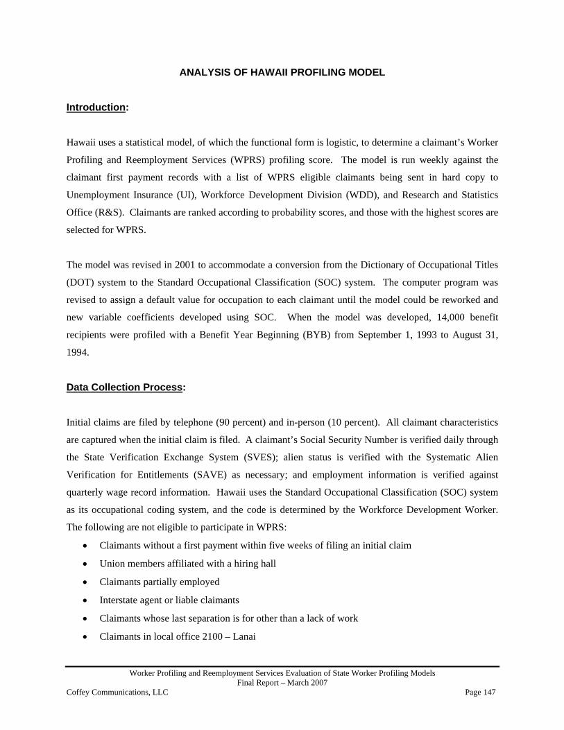
Worker Profiling and Reemployment Services Evaluation of State Worker Profiling Models Final Report – March 2007
Coffey Communications, LLC Page 147
ANALYSIS OF HAWAII PROFILING MODEL
Introduction: Hawaii uses a statistical model, of which the functional form is logistic, to determine a claimant’s Worker
Profiling and Reemployment Services (WPRS) profiling score. The model is run weekly against the
claimant first payment records with a list of WPRS eligible claimants being sent in hard copy to
Unemployment Insurance (UI), Workforce Development Division (WDD), and Research and Statistics
Office (R&S). Claimants are ranked according to probability scores, and those with the highest scores are
selected for WPRS.
The model was revised in 2001 to accommodate a conversion from the Dictionary of Occupational Titles
(DOT) system to the Standard Occupational Classification (SOC) system. The computer program was
revised to assign a default value for occupation to each claimant until the model could be reworked and
new variable coefficients developed using SOC. When the model was developed, 14,000 benefit
recipients were profiled with a Benefit Year Beginning (BYB) from September 1, 1993 to August 31,
1994.
Data Collection Process: Initial claims are filed by telephone (90 percent) and in-person (10 percent). All claimant characteristics
are captured when the initial claim is filed. A claimant’s Social Security Number is verified daily through
the State Verification Exchange System (SVES); alien status is verified with the Systematic Alien
Verification for Entitlements (SAVE) as necessary; and employment information is verified against
quarterly wage record information. Hawaii uses the Standard Occupational Classification (SOC) system
as its occupational coding system, and the code is determined by the Workforce Development Worker.
The following are not eligible to participate in WPRS:
• Claimants without a first payment within five weeks of filing an initial claim
• Union members affiliated with a hiring hall
• Claimants partially employed
• Interstate agent or liable claimants
• Claimants whose last separation is for other than a lack of work
• Claimants in local office 2100 – Lanai

Worker Profiling and Reemployment Services Evaluation of State Worker Profiling Models Final Report – March 2007
Coffey Communications, LLC Page 148
Selection/Referral Process:
Individuals selected for WPRS are referred by hard copy listings. The number of individuals to be served
is determined by the center based on available resources. Claimants are ranked according to probability
scores with the highest scores being selected first. Workforce center staff can also manually select
claimants from the list if openings exist.
Profiling Model Structure:
The WPRS profiling model employed by Hawaii utilizes a statistical model, of which the functional form
is logistic, to estimate benefit exhaustion. The dependent variable is benefit exhaustion defined as the
payment of the maximum benefit amount. The independent variables are as follows:
• Education
• Job Tenure
• Industry
• Occupation
• Local Unemployment Rate
Profiling Model Performance:
Hawaii provided their survey, a dataset and the model structure. Included in the dataset was a binary
variable indicating whether or not benefit recipients were referred to reemployment services. This binary
variable allows us to test for endogeneity within our data and answer the question - does referral to
reemployment services have an effect on the exhaustion of benefits?
Our first step was to try to replicate the given score using the data provided and the coefficients for the
variables given. From the given data, we were able to replicate the original score, creating a score that
correlated with the provided score at 0.86. However, to do so we had to delete four cases with erroneous
values for the profiling score.
We used the profiling scores provided to produce a decile table as shown below. The decile means are
calculated by dividing the percentage of recipients that exhaust benefits for a given decile by 100. For
example, in the first decile, our mean is 0.327, or approximately 33 percent, which indicates that
approximately 33 percent of benefit recipients in this decile exhausted benefits.
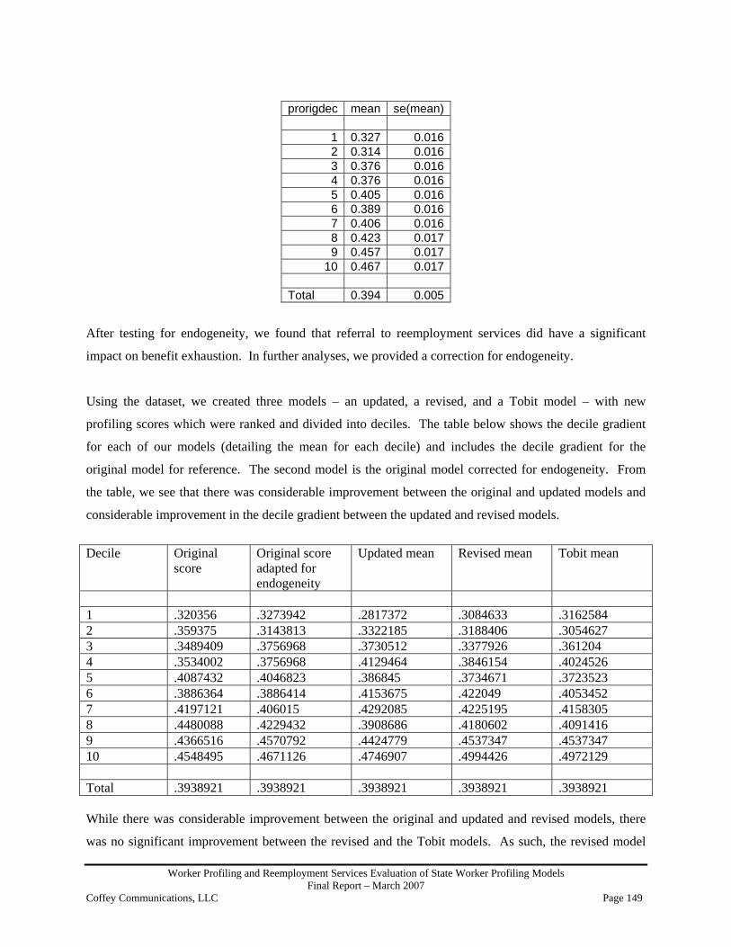
Worker Profiling and Reemployment Services Evaluation of State Worker Profiling Models Final Report – March 2007
Coffey Communications, LLC Page 149
prorigdec mean se(mean)
1 0.327 0.0162 0.314 0.0163 0.376 0.0164 0.376 0.0165 0.405 0.0166 0.389 0.0167 0.406 0.0168 0.423 0.0179 0.457 0.017
10 0.467 0.017 Total 0.394 0.005
After testing for endogeneity, we found that referral to reemployment services did have a significant
impact on benefit exhaustion. In further analyses, we provided a correction for endogeneity.
Using the dataset, we created three models – an updated, a revised, and a Tobit model – with new
profiling scores which were ranked and divided into deciles. The table below shows the decile gradient
for each of our models (detailing the mean for each decile) and includes the decile gradient for the
original model for reference. The second model is the original model corrected for endogeneity. From
the table, we see that there was considerable improvement between the original and updated models and
considerable improvement in the decile gradient between the updated and revised models.
Decile Original
score Original score adapted for endogeneity
Updated mean Revised mean Tobit mean
1 .320356 .3273942 .2817372 .3084633 .3162584 2 .359375 .3143813 .3322185 .3188406 .3054627 3 .3489409 .3756968 .3730512 .3377926 .361204 4 .3534002 .3756968 .4129464 .3846154 .4024526 5 .4087432 .4046823 .386845 .3734671 .3723523 6 .3886364 .3886414 .4153675 .422049 .4053452 7 .4197121 .406015 .4292085 .4225195 .4158305 8 .4480088 .4229432 .3908686 .4180602 .4091416 9 .4366516 .4570792 .4424779 .4537347 .4537347 10 .4548495 .4671126 .4746907 .4994426 .4972129 Total .3938921 .3938921 .3938921 .3938921 .3938921 While there was considerable improvement between the original and updated and revised models, there
was no significant improvement between the revised and the Tobit models. As such, the revised model

Worker Profiling and Reemployment Services Evaluation of State Worker Profiling Models Final Report – March 2007
Coffey Communications, LLC Page 150
appears to be the best model using the data available (see detail on revised model in Appendix D). We
tested the performance of each model using the following metric:
Percent exhausted of the top 39.4% of individuals in the score.
We used 39.4 percent because the exhaustion rate for benefit recipients in the Hawaii dataset was 39.4
percent. This metric will vary from about 39.4 percent, for a score that is a random draw, to 100 percent
for a score that is a perfect predictor of exhaustion. The scores for the four models are as follows:
Score % exhausted of those with the top 39.3% of score Standard error of the scoreOriginal 43.87408 .83581 Adapted 43.87408 .83581 Updated 43.2785 .83451 Revised 44.81293 .83737 TOBIT 44.36281 .83524
In the metric below, “Exhaustion” is the percentage of all benefit recipients in our sample that exhaust
benefits. For Hawaii, “Exhaustion” is 39.4 percent since the exhaustion rate for all benefit recipients in
the provided dataset was 39.4 percent. “Pr[Exh]” in our metric is determined by the model with the
highest percentage of benefit exhaustees with profiling scores falling in the top X percent of the sample,
where X percent is determined by the exhaustion rate for all benefit recipients in the sample. For Hawaii,
“Pr[Exh]” is represented by the revised model with a score of 44.81 percent for benefit recipients who
exhaust benefits with scores falling in the top 39.4 percent.
100 – Pr[Exh] Metric: 1 – 100 – Exhaustion
We used the numbers above to calculate a score of 0.069 for the original profiling score (corrected for
endogeneity) and a score of 0.085 for the revised score.
SWA Profiling
score Control for
endogeneity? Exhaustion rate for the
state
Number of individuals
with the highest profiling score
Exhaustion rate for
individuals with high profiling scores
Metric Variance of the Metric
Standard Error of
the metric
Hawaii original score
Y 39.7 3,526 43.9 0.069 1.248 0.019
Hawaii revised score
Y 39.7 3,526 44.8 0.085 1.232 0.019

Worker Profiling and Reemployment Services Evaluation of State Worker Profiling Models Final Report – March 2007
Coffey Communications, LLC Page 151
These metrics show that the revised model is significantly better that the original score. The metrics also
show a baseline on which other models can improve. Further analysis of Hawaii’s model is in the
expanded analysis section.

Worker Profiling and Reemployment Services Evaluation of State Worker Profiling Models Final Report – March 2007
Coffey Communications, LLC Page 152
ANALYSIS OF IDAHO PROFILING MODEL
Introduction:
Idaho uses a characteristic screen to determine a claimant’s eligibility for selection and referral to Worker
Profiling and Reemployment Services (WPRS). The model is run weekly against the claimant first
payment records with a list of WPRS eligible claimants sent to consultants in the 24 local offices. The
consultants use the list to contact potential candidates and make a decision on how best to serve each
candidate.
The model is updated annually, and a major revision was implemented in June, 2005 when independent
variable relationships were analyzed and revised as necessary.
Data Collection Process:
Initial claims are filed in-person (5 percent), by telephone (6 percent) and Internet (89 percent). Claimant
characteristics that determine an individual’s eligibility for WPRS are captured at the same time the initial
claim is taken. Claimants self-select the occupational code using the SOC classification system. UI wage
records are checked to determine the claimant’s industry code. Individuals not eligible for selection and
referral to WPRS include:
• Claimants who are empoloyer attached
• Claimants who are union hiring hall attached
• Claimants who are on a short-term layoff of 16 weeks or less
Selection/Referral Process:
The profiling candidate list is available for viewing online by staff in the 24 local centers. Claimants with
a probability of exhaustion score of 50 percent or above are selected for services. Local offices have
discretion on selection of the candidates within the 50 – 100 percent rankings. Each office’s management
staff, in conjunction with area managers and their chain of command, determines a target number of
claimants to serve at the start of the year. That number is periodically reviewed and revised to ensure
target groups and individuals are properly identified for referral to services.

Worker Profiling and Reemployment Services Evaluation of State Worker Profiling Models Final Report – March 2007
Coffey Communications, LLC Page 153
Profiling Model Structure:
The WPRS profiling model employed by Idaho to estimate benefit exhaustion is a characteristic screen
model called a “decision tree.” The model’s dependent variable is benefit exhaustion, defined as
maximum benefits paid (i.e., when a claimant’s remaining benefit balance is $40), and the independent
variables examined in the screen are as follows:
• Potential Duration of Benefit Receipt
• NAICS (21 separate industries at the sector level are used)
• County of Residence/Local Office Federal Information Processing Standards (FIPS) Code
• Marital Status
• Job Tenure
• WBA
• Ratio of Total Wage to High Quarter Wage
• Number of Employers
• Education (years completed)
• Month of Filing
Records with missing values are kept and processed as missing, thus assuring that no qualifying records
are excluded from the modeling process.
Profiling Model Performance:
Idaho provided both a dataset for data analysis and their model structure for revision. The Idaho model
used 31 combinations of their independent variables to define groups of individuals to be selected for
referral to reemployment services. For example, the first group was defined as individuals having a
duration greater than 16; a principal industry of 1 (a NAICS of 0, or no reported industry); a county of
residence of FIPS code 1, 19, 27, 35, 69, 75, or 79; and a ratio of total wage to high quarter wage of
between 2.34 and 2.68. Individuals who belonged to any one of the 31 groups were selected for
reemployment services. In the sample given, 73 percent of the individuals were selected.
This approach has both strengths and weaknesses. The model can be tailored to various subsets of
applicants. That is, individuals with a principal industry of 2 are selected very differently from
individuals with a principal industry of 7. However, the model also could leave out many individuals
who are likely to exhaust and/or select individuals who are not likely to exhaust. For example,

Worker Profiling and Reemployment Services Evaluation of State Worker Profiling Models Final Report – March 2007
Coffey Communications, LLC Page 154
individuals with a principal industry of 1 are not selected on the basis of any variable except duration and
county of residence. Inclusion of other variables in the selection process for individuals with a principal
industry of 1 would probably improve the model.
The first step of our analysis is to calculate a new selection variable. The current selection variable takes
a value of zero or one. We used the same variables in the decision tree to calculate a continuous selection
variable. The higher values of this new selection variable would correspond to the “ones” of the original
selection variable; lower values of this new selection variable would correspond to the “zeros” of the
original selection variable.
Our method is to run a logistic regression model with the variables listed above as independent variables
and the original selection variable as dependent variable. Due to collinearity problems, we eliminated
principal industry 1, FIPS 1 (county 1), month 1, Duration (correlated at 0.9789 with RATIO), Weekly
Benefit Amount (WBA) [correlated at 0.8572 with Total Benefit Amount (TBA)]. By taking the
predictions of this model, ordering them and dividing them into deciles, and then for each decile, showing
the actual exhaustion rate along with its standard error, we obtain the following table.
Decile Mean Standard Error (Mean) 1 .411 .00844162 .393 .00837953 .365 .00825774 .359 .00823345 .35 .00818126 .362 .00824347 .438 .00851338 .55 .00853279 .65 .008181210 .709 .0077873 Total .459 .0027027 Note: the results above are adjusted for endogeneity. A thorough explanation of our methods for testing
and adjusting for endogeneity is included in the expanded analysis included in our technical report.
This decile table is the basis for demonstrating the effectiveness of each model. The decile means are
calculated by dividing the percentage of recipients that exhaust benefits for a given decile by 100. For
example, in the first decile our mean is 0.411, which indicates that approximately 41 percent of benefit
recipients in this decile exhausted benefits.

Worker Profiling and Reemployment Services Evaluation of State Worker Profiling Models Final Report – March 2007
Coffey Communications, LLC Page 155
Using the Idaho dataset, we continued our analysis of the SWA’s profiling model by creating three
models – an updated, a revised, and a Tobit model. For each of the models, new profiling scores were
created, ranked, and divided into deciles. The table below shows the decile gradient for each model
(detailing the mean for each decile) and includes the decile gradient for the original model for reference.
From the table, there was an improvement between the original and updated models and further
improvement in the decile gradient between the updated and revised models.
Decile Original score Updated score Revised score Tobit score 1 .411 .219 .216 .2272 .393 .304 .297 .3193 .365 .353 .359 .3534 .359 .389 .391 .3935 .35 .435 .424 .4186 .362 .444 .459 .4467 .438 .504 .50 .5028 .55 .566 .565 .5529 .65 .643 .642 .63410 .709 .729 .734 .741 Total .459 .459 .459 .459 While there was improvement between the original and updated and revised models, there was no
apparent improvement between the revised and the Tobit models. The revised model appears to be the
best model using the data available (see Appendix D for information on revised model). Additionally, we
tested the performance of each model using the following metric:
Percent exhausted of the top 45.9% of individuals in the score.
We used 45.9 percent because the exhaustion rate for benefit recipients in the dataset provided by Idaho
was 45.9 percent. This metric will vary from about 45.9 percent, for a score that is a random draw, up to
100 percent for a score that is a perfect predictor of exhaustion. The scores for the four models are as
follows:
Score % exhausted of those with the top 45.9% of score Standard error of the score Original 56.1 0.39729 Updated 59.03 0.39367 Revised 59.26 0.39335 Tobit 58.82 0.39399

Worker Profiling and Reemployment Services Evaluation of State Worker Profiling Models Final Report – March 2007
Coffey Communications, LLC Page 156
We note that the revised model performed better than the updated and Tobit models. The original model
performed worst, and the Tobit model performed slightly worse than the updated model.
In the metric below, “Exhaustion” is the percentage of all benefit recipients in the sample that exhaust
benefits. For Idaho, “Exhaustion” is 45.9 percent since the exhaustion rate for all benefit recipients in the
provided dataset is 45.9 percent. “Pr[Exh]” in our metric is determined by the model with the highest
percentage of benefit exhaustees with profiling scores falling in the top X percent of the sample, where X
percent is determined by the exhaustion rate for all benefit recipients in the sample. For Idaho, “Pr[Exh]”
is represented by the revised model with a score of 59.26 percent for benefit recipients that exhaust
benefits with scores falling in the top 45.9 percent.
100 – Pr[Exh] Metric: 1 – 100 – Exhaustion
We used the numbers above to calculate a metric of 0.189 for the estimated original profiling score
(corrected for endogeneity) and a score of 0.247 for the revised score.
SWA Profiling
score Control for
endogeneity? Exhaustion rate for the
state
Number of individuals
with the highest profiling score
Exhaustion rate for
individuals with high profiling scores
Metric Variance of the Metric
Standard Error of
the metric
Idaho estimated score* Y 45.9 15,605 56.1 0.189 1.400 0.009
Idaho revised score
Y 45.9 15,605 59.3 0.247 1.306 0.009
These metrics show that the revised model is significantly better that the estimated original score. The
metrics also show a baseline on which other models can improve. Further analysis of Idaho’s model is in
the expanded analysis section below.

Worker Profiling and Reemployment Services Evaluation of State Worker Profiling Models Final Report – March 2007
Coffey Communications, LLC Page 157
ANALYSIS OF ILLINOIS PROFILING MODEL
Introduction: Illinois uses a statistical model, of which the functional form is logistic, to determine a claimant’s Worker
Profiling and Reemployment Services (WPRS) profiling score. The model is run weekly against the
claimant first payment records, and a listing of WPRS eligible claimants is sent electronically or by fax to
Local Workforce Investment Areas (LWIA). This list ranks the candidates in order from the highest
probability of exhaustion to the lowest, and the LWIAs determine the number of profiling candidates to
be served based on resources currently available. The model was updated in 1997 but has never been
revised.
Data Collection Process: Initial claims are filed in person (80 percent) and through the Internet (20 percent). Claimant
characteristics data are captured at the time the initial claim is filed, and there are no further checks for
accuracy. The initial claims taker assigns the claimant’s occupational code using the Dictionary of
Occupational Titles (DOT) system. The claimant’s primary employer, used in assigning the industry
code, is determined by a review of the claimant’s wage records. The following claimants are not eligible
for WPRS services:
• Claimants who do not receive a first payment
• Claimants registered with a union hiring hall
• Claimants with a return to work date
• Claimants who leave work voluntarily
• Claimants involved in a labor dispute
Selection/Referral Process: A listing of WPRS eligible claimants is sent to LWIAs electronically or by fax. This list ranks the
candidates in order from the highest probability of exhaustion to the lowest, and the LWIAs determine the
number of profiling candidates to be served based on the resources available. LWIAs cannot “skip down
the rank” in selecting candidates for services. The candidates must be served in order of their probability
of exhaustion.

Worker Profiling and Reemployment Services Evaluation of State Worker Profiling Models Final Report – March 2007
Coffey Communications, LLC Page 158
Profiling Model Structure:
The WPRS profiling model utilizes a statistical model, of which the functional form is logistic, to
estimate benefit exhaustion. The dependent variable is exhaustion of benefits, defined as the payment of
the maximum benefit amount. The independent variables are as follows:
• Reason for Unemployment
• Tenure
• Occupation
• Filing Lag
Profiling Model Performance: Illinois did not provide a dataset for data analysis and/or model revision; therefore, we were unable to
gauge the performance of its current model.

Worker Profiling and Reemployment Services Evaluation of State Worker Profiling Models Final Report – March 2007
Coffey Communications, LLC Page 159
ANALYSIS OF INDIANA PROFILING MODEL
Introduction: Indiana uses a statistical model, of which the functional form is logistic, to determine a claimant’s Worker
Profiling and Reemployment Services (WPRS) profiling score. The model is run weekly against the
claimant first payment records, and a listing of WPRS-eligible claimants is produced at that time and
electronically distributed to local office staff. Local office managers determine the number of eligible
claimants to be served based on staffing resources. The listing ranks claimants in order from the highest
to the lowest probability of exhaustion, and the local office cannot deviate from the listing. The model
has never been updated or revised.
Data Collection Process: Initial claims are filed in-person and by Internet. Claimant characteristics are captured at the time the
initial claim is filed. Only the claimant’s social security number is verified for accuracy. Both the
occupational and industry codes are assigned based on the claimant’s work history, and the following
claimants are not eligible for WPRS services:
• Job Attached
• Union Members
• Claimants Filing Trade Adjustment Assistance Claims
Selection/Referral Process: Claimants selected for WPRS are ranked from those with the highest probability of exhaustion to the
lowest. A listing is produced that is distributed electronically to the local offices. Local office managers
determine the number of WPRS candidates to be called in and served based on staff resources available.
Claimants with the highest probability of exhaustion must be called in first.
Profiling Model Structure: The WPRS profiling model employed by Indiana utilizes a statistical model, of which the functional form
is logistic, to estimate benefit exhaustion. The dependent variable is benefit exhaustion, defined as the
payment of the maximum benefit amount. The independent variables are as follows:

Worker Profiling and Reemployment Services Evaluation of State Worker Profiling Models Final Report – March 2007
Coffey Communications, LLC Page 160
• Education
• Maximum Benefits
• Occupation
• Annualized County Unemployment Rate
• Months of Tenure
Extensive testing of several variables, including those listed above, occurred prior to model
implementation. The variables found not to impact benefit exhaustion were industry, county growth rate,
projected Standard Industrial Classification (SIC) growth rate, weekly benefit amount, claim balance
remaining, and variations of occupational classification such as the projected Dictionary of Occupational
Titles (DOT) growth rate.
Profiling Model Performance: Indiana did not provide a dataset for data analysis and/or model revision; therefore, we were unable to
gauge the performance of its current model.

Worker Profiling and Reemployment Services Evaluation of State Worker Profiling Models Final Report – March 2007
Coffey Communications, LLC Page 161
ANALYSIS OF IOWA PROFILING MODEL
Introduction: Iowa uses a statistical model, of which the functional form is logistic, to determine a claimant’s Worker
Profiling and Reemployment Services (WPRS) profiling score. The model is run weekly against the
claimant first payment records. A listing of all profiled claimants is produced when claimants are
selected for orientation to reemployment services. The number of individuals to be called in for services
is determined by workforce center administrators based on staff resources and facility availability. Local
regions have flexibility in this regard but are assigned an annual goal for the number of individuals to be
served. This goal is set by Unemployment Insurance (UI) and Workforce Development administrators.
The model has never been updated or revised.
Data Collection Process:
Initial claims are filed in-person (46 percent), by telephone (31 percent), through employer filed mass
claims (4 percent) and via Internet (20 percent). Internet claims include those filed by claimants using
local office resource room computers. Claimant characteristic data are collected at the time the initial
claim is taken, and there are no checks on the accuracy of the information supplied by the claimant.
Dictionary of Occupational Titles (DOT) system codes are assigned to claimants and are subsequently
converted to Standard Occupational Classification (SOC) system codes that use a crosswalk when the
model is run. The industry code is based on the claimant’s last employer as indicated on the initial claim.
Claimants ineligible for referral to services through profiling include:
• Claimants who are job attached (likely to return to last employer)
• Claimants on temporary layoff
• Claimants who refused to bump less senior employees
• Claimants who obtain work through a union hiring hall
• Work-share claimants
• Claimants with an out-of-state address
Workforce center staff may exempt claimants from participation in reemployment services if they:
• were referred in error (obtained work through a union hiring hall, definite date of recall with
former employer)
• are currently participating in a similar service
• have completed reemployment services or a job training program in the last six months

Worker Profiling and Reemployment Services Evaluation of State Worker Profiling Models Final Report – March 2007
Coffey Communications, LLC Page 162
• are currently attending training under a department approved training program
Selection/Referral Process:
A file of claimants eligible for WPRS services is generated at the time of first payment; however, a list of
eligible claimants is not created until they are selected for a reemployment services orientation session.
When there is a need to refer individuals to the workforce centers, a notice to appear is generated from the
central office and a listing of notified individuals is sent to the local profiling coordinators. A statewide
goal of the number of profiled candidates to be served is determined by UI and Workforce Development
administrators. The goal is to distribute candidates to local regions based on their historic share of
claimants who are not job attached. Local regions have flexibility in determining the size and frequency
of candidate selection and their orientation sessions. These determinations are based on staff resources
and facility availability.
Profiling Model Structure:
The WPRS profiling model utilizes a statistical model, of which the functional form is logistic, to
estimate benefit exhaustion. The dependent variable is benefit exhaustion defined by payment of the
maximum benefit amount. The independent variables are as follows:
• Education
• Job Tenure
• Twelve-month Statewide Industry Growth (based on published NAICS or SIC sectors)
• Growing/Declining Occupation (national one digit SOC)
• Local Region Unemployment Rate
Profiling Model Performance: Iowa provided the model structure and dataset for data analysis but did not provide useable data for state
industry growth, decreasing and increasing occupation factors, and regional unemployment rate.
Therefore, we did not conduct an extended analysis for Iowa. We did calculate a decile table for Iowa
with a correction for endogeneity. It is shown below.

Worker Profiling and Reemployment Services Evaluation of State Worker Profiling Models Final Report – March 2007
Coffey Communications, LLC Page 163
prorigdec mean se(mean)
1 0.145 0.0082 0.152 0.0048 0.162 0.0109 0.156 0.010
10 0.170 0.010 Total 0.154 0.003
Note that, due to large numbers of individuals with the same score, we were not able to separate the
sample into 10 parts. We also calculated the metric that shows the effectiveness of Iowa’s profiling score.
It is shown below.
SWA Profiling score
Control for endogeneity?
Exhaustion rate for the
state
Number of individuals
with the highest profiling score
Exhaustion rate for
individuals with high profiling scores
Metric Variance of the Metric
Standard Error of
the metric
Iowa original score
Y 15.4 2,456 16.2 0.010 0.368 0.012
The metric has a value of 0.010 and a standard error of 0.012. The metric is not really useful because it is
not significantly greater than 0. However, further analysis may result in a better model. The metric
provides a basis for comparison with other profiling models.

Worker Profiling and Reemployment Services Evaluation of State Worker Profiling Models Final Report – March 2007
Coffey Communications, LLC Page 164
ANALYSIS OF KANSAS PROFILING MODEL
Introduction: Kansas uses a statistical model, of which the functional form is logistic, to determine a claimant’s Worker
Profiling and Reemployment Services (WPRS) profiling score. The model is run daily against the
claimant first payment records, and a listing of WPRS eligible claimants is mailed to local centers and
provided on the Job Link website. This list ranks candidates in order from highest probability of
exhaustion to lowest. There has been no update or revision to the model since its creation in 1995.
Data Collection Process:
Initial claims are filed by telephone (75 percent) and Internet (25 percent) with claimant characteristics
captured at the time initial claims are filed. A Workforce Development worker assigns the occupation
code using the Standard Occupational Classification (SOC) system derived from the O*Net classification
system. For purposes of assigning North American Industrial Classification System (NAICS)/Standard
Industrial Classification (SIC) system codes, the primary employer is determined by a review of the
claimant’s work history. Individuals not eligible for referral to services through WPRS include:
• Union Workers
• Claimants Awaiting Job Recall
• Claimants in Approved Training
Note: currently there are no checks on the accuracy of the information provided by the claimant and all
incomplete records are ignored.
Selection/Referral Process:
The list of WPRS eligible candidates is produced at the same time that the profiling model is run. The list
is mailed to the local centers and provided on the Job Link website. Workforce Development staff
determine the number of candidates to call in based on their workload. Individuals are ranked from high
to low probabilities of exhaustion and the ranked listings are provided to Workforce Development staff.
Under no conditions does the local area skip candidates.

Worker Profiling and Reemployment Services Evaluation of State Worker Profiling Models Final Report – March 2007
Coffey Communications, LLC Page 165
Profiling Model Structure:
The WPRS profiling model utilizes a statistical model, of which the functional form is logistic, to
estimate benefit exhaustion. The dependent variable is benefit exhaustion defined as full payment of the
maximum benefit amount. The independent variables include:
• Years of Experience
• County Total Unemployment Rate
• Wage Replacement Rate
• Metropolitan Statistical Area or Non-Metro Area
• One-digit SIC Code
The variables for years of experience, county total unemployment rate, and wage replacement amount are
all categorical variables. They are:
• Four categories for years of experience: less than three years, three to four years, five to seven
years, and eight or more years of experience
• Three categories for county total unemployment rate: 0 to 5 percent, 5.1 to 8 percent, and 8.1
percent or above
• Five categories for wage replacement rates: 0.0 to 0.0100, 0.0101 to 0.015, 0.0151 to 0.02, 0.0201
to 0.025, and 0.0251 and above
Profiling Model Performance: Kansas did not provide a dataset for data analysis and/or model revision; therefore, we were unable to
gauge the performance of its current model.

Worker Profiling and Reemployment Services Evaluation of State Worker Profiling Models Final Report – March 2007
Coffey Communications, LLC Page 166
ANALYSIS OF KENTUCKY PROFILING MODEL
Introduction: Kentucky uses a statistical model, of which the functional form is Tobit, to determine a claimant’s
eligibility for selection and referral to Worker Profiling and Reemployment Services (WPRS). In June,
1994, Kentucky was selected by the Employment and Training Administration to be a prototype state for
the development of a system for profiling Unemployment Insurance (UI) claimants. The Center for
Business and Economic Research (CBER) at the University of Kentucky developed a profiling system for
the Department for Employment Services (DES). This system generated a single score for each claimant
to measure the probability of a claimant exhausting his or her benefits. The model was updated in 1997
and has never been revised. It is run weekly against the claimant first payment file, and the resulting list
of profiled claimants sent via an encrypted e-mail list to the local offices.
Data Collection Process: Initial claims are filed by telephone and by Internet. Claimant characteristic data are captured at the time
the claim is filed and is confirmed by Social Security Number through the State Verification and
Exchange System (SVES). Employers and addresses are verified by mail, and the reason of separation is
verified with the employer.
Selection/Referral Process:
The list of claimants eligible for WPRS is produced when the weekly WPRS model is run and is
distributed to the Kentucky DES local offices via an encrypted e-mail. Eligible claimants are listed by
office, and those claimants having the highest probability of exhaustion are at the top of the list.
Claimants must be selected in descending order as there are no provisions for choosing claimants out of
order. The Director of the Division for Workforce and Employment Services determines the number of
eligible candidates to be called in weekly based on the service capacity of the office (i.e., after
considering available space and staffing levels).

Worker Profiling and Reemployment Services Evaluation of State Worker Profiling Models Final Report – March 2007
Coffey Communications, LLC Page 167
Profiling Model Structure: The WPRS profiling model utilizes a Tobit functional form to estimate benefit exhaustion. The dependent
variable is benefit exhaustion, defined as maximum benefits paid. The independent variables were
created using five years of claimant data obtained from the UI computer mainframe database. Variables
from the Enhanced National Data System (ENDS), the U.S. Bureau of Economic Analysis’ Regional
Economic Information System (REIS), the 1990 U.S. Census and the ES-202 database were also included
in the analysis. Those ultimately selected include:
• Monetary Variables (annual wage, benefit amount, reservation wage)
• Demographic Variables (Does the worker have a phone? Is the worker economically disadvantaged?
Is the worker on welfare? Does the worker hold a driver’s license?)
• Industry Code (SIC codes)
• Education Variables (level of education)
• Occupation Variables (accessed from the ENDS database)
• Characteristics of Job Variables (tenure – also derived from the ENDS database)
• Prior UI Receipt Variables
• Variables to Capture Regional Economic Differences
Profiling Model Performance: Kentucky did not provide a dataset for data analysis and/or model revision; therefore, we were unable to
gauge the performance of its current model.

Worker Profiling and Reemployment Services Evaluation of State Worker Profiling Models Final Report – March 2007
Coffey Communications, LLC Page 168
ANALYSIS OF LOUISIANA PROFILING MODEL
Introduction: Louisiana uses a statistical model, of which the functional form is logistic, to determine a claimant’s
eligibility for referral to Worker Profiling and Reemployment Services (WPRS). The model is run
weekly against the claimant first payment records with a list of WPRS eligible claimants made available
to both Wagner-Peyser and Workforce Investment Act (WIA) staff by Job Center and Local Workforce
Investment Area (LWIA). Claimants remain in the selection pool for four weeks before they are deleted.
Louisiana undertook a major revision of its profiling model in June, 2003. This revision included the
following:
• Updating for changes in economic conditions since 1999
• Change from Dictionary of Occupational Titles (DOT) system to Standard Occupational
Classification (SOC) system
• Change from the Standard Industrial Classification (SIC) to the North American Industry
Classification System (NAICS) industry coding
• Change to a logit model, addition of new variables, and allowing for nonlinear relationships.
The revised model was developed by the Division of Economic Development and Forecasting at
Louisiana State University. The model was developed based on a sample of 85,284 benefit recipients.
Data Collection Process:
Initial claims are filed in-person (5 percent) and by Internet (95 percent). Claimant characteristic data are
captured at the time the claim is filed, and there are no further checks on the accuracy of the information.
When the claim is filed by Internet, the claimant self-selects the occupational (SOC) and industrial codes
[North American Industry Classification System (NAICS)]. When filing in-person, the claims taker
assigns the occupational and industrial codes. O*Net occupational coding is used in the WIA One-Stops.
The following individuals are not eligible for referral to WPRS:
• Union members
• Work attached claimants
• Interstate claimants
• Claimants in approved training

Worker Profiling and Reemployment Services Evaluation of State Worker Profiling Models Final Report – March 2007
Coffey Communications, LLC Page 169
• Claimants who completed or are participating in similar services
• Claimants with justifiable cause
• Claimants who have received more than five weeks of benefits.
Selection/Referral Process: The list is available on the mainframe through screens for Wagner-Peyser and WIA staff. Local staff
determines the number of candidates to be served based on the type of services needed, available space
and staff capacity. The listing is sorted in the order of those having the highest probability of exhaustion
to lowest. Generally, the profiled claimants with the highest probabilities are called in and served first.
Local staff persons have discretion to select at will, and may select claimants whom they determine need
additional services even though the claimants have been seen previously. This occurs most frequently
with claimants who are in the pool and their four week limitation is about to expire. The WIA One-Stops
use O*Net occupational coding.
Profiling Model Structure: The WPRS profiling model employed by Louisiana utilizes a logistic regression model to estimate benefit
exhaustion. The dependent variable is benefit exhaustion, defined as maximum benefits paid. The
independent variables are as follows:
• Occupation
• Industry
• Regional labor market unemployment rate
• Education
• Number of days between the separation from work date and the initial claim filing date
• Exhaustion of benefits on a prior claim
• Average unemployment compensation received
• Replacement ratio (ratio of benefits paid to average wage)
• Number of employers in the base period.
As noted above, four possible models were considered for adoption.

Worker Profiling and Reemployment Services Evaluation of State Worker Profiling Models Final Report – March 2007
Coffey Communications, LLC Page 170
Profiling Model Performance:
Louisiana provided the model structure and dataset for data analysis but did not provide useable data for
occupation, regional labor market unemployment rate, number of days between the separation from work
date and the initial claim filing date, and number of employers in the base period. Therefore, we did not
conduct an extended analysis for Louisiana. We did calculate a decile table with a correction for
endogeneity. It is shown below.
prorigdec mean se(mean)
1 0.325 0.0062 0.322 0.0063 0.341 0.0064 0.383 0.0075 0.407 0.0076 0.383 0.0077 0.477 0.0078 0.500 0.0079 0.505 0.007
10 0.621 0.007 Total 0.426 0.002
We also calculated the metric that shows the effectiveness of Louisiana’s profiling score. It is shown
below.
SWA Profiling score
Control for endogeneity?
Exhaustion rate for the
state
Number of individuals
with the highest profiling score
Exhaustion rate for
individuals with high profiling scores
Metric Variance of the Metric
Standard Error of
the metric
Louisiana original score
Y 42.6 22,825 51.9 0.161 1.282 0.007
The metric has a value of 0.161 and a standard error of 0.007. The metric is useful because it is
significantly greater than 0. The metric provides a basis for comparison with other profiling models.

Worker Profiling and Reemployment Services Evaluation of State Worker Profiling Models Final Report – March 2007
Coffey Communications, LLC Page 171
ANALYSIS OF MAINE PROFILING MODEL
Introduction: Maine uses a statistical model, of which the functional form is logistic, to determine a claimant’s profiling
score for identification and referral to Worker Profiling and Reemployment Services (WPRS). The model
is run weekly against the claimant first payment records, and with a list of WPRS eligible claimants is
sent in hard copy to the Bureau of Employment Services for distribution to the One-Stop Centers. This
list ranks candidates in order from highest probability of exhaustion to lowest. The One-Stops determine
who is called in based on capacity and claimants with the highest likelihood of exhaustion.
The model was revised in 2000 and 2004. The first revision to the model was implemented on January 1,
2000. During this revision, the “Education,” “Reason Unemployed,” and “Ratio of High Quarter Wages
to Base Period Wages” variables were eliminated, and the “Job Tenure” variable was added.
The second revision to the model was implemented on September 1, 2004. The changes were extensive
and included:
• Change from Standard Industrial Classification (SIC) to North American Industry
Classification System (NAICS) (industry change at 3-digit NAICS level by County)
• Binary Industry Variable at Super Sector Level
• Addition of an “Effective Quarter of Claim” variable
• Addition of a “Number of Base Period Employers” variable
• Addition of a “Separation Reason” variable
• Addition of a “Ratio of High Quarter Wages to Base Period Wages” variable
• Addition of an “Education” variable
• Removal of occupation variables
Data Collection Process: Initial claims are filed by telephone, mail and Internet. Automated and manual records are used to assist
in classifying individuals for WPRS, with claims takers determining the occupational codes of individuals
filing telephonically and by mail; these codes are self-selected by claimants when filings are made via the
Internet. The DOT code system is used to classify the occupational codes. The NAICS code is obtained
from each claimant’s wage record and is determined by their last employer. There are no further checks

Worker Profiling and Reemployment Services Evaluation of State Worker Profiling Models Final Report – March 2007
Coffey Communications, LLC Page 172
on the accuracy of information provided by the claimant. Individuals not eligible for referral to services
through WPRS include:
• Interstate Claimants
• Claimants with a recall date; or those expecting to be recalled
• Claimants who obtain employment through a union hiring hall
• Claimants without a first payment
Selection/Referral Process: Claimants eligible for services through WPRS are selected when they receive their first payment. They
are then ranked with claimants with the highest probability of exhausting benefits appearing first. The list
of eligible claimants is sent to the Bureau of Employment Services for distribution to the Career Centers
(One-Stops) by interoffice mail. Each Career Center determines the number of profiled claimants that it
can serve for a specified period of time. Those with the next highest exhaustion probability scores are
selected until all of available slots are filled for each Center. The Centers are not given the option of who
to serve; they must adhere to the ranking on the list. There are no feedback loops in place.
Profiling Model Structure: The dependent variable is benefit exhaustion, defined as the payment of the maximum benefit amount.
The revision of January 1, 2000 utilized a sample of 14,969 benefit recipients to determine the needed
changes. The revision of September 1, 2004 utilized a sample of 17,537 benefit recipients to determine
the needed changes. Prior to implementation, the original model was based on a sample of approximately
9,000 benefit recipients. The independent variables are as follows:
• NAICS Code (industry change at 3-digit NAICS level by county)
• Binary Industry Variable at Super Sector Level
• Effective Quarter of Claim
• Number of Base Period Employers
• Separation Reason
• Ratio of High Quarter Wages to Base Period Wages
• Years of Education
In order to select the independent variables when WPRS was initially implemented, a Statistical Analysis
System (SAS) or National Council for Social Studies (NCSS) software package was used to evaluate the

Worker Profiling and Reemployment Services Evaluation of State Worker Profiling Models Final Report – March 2007
Coffey Communications, LLC Page 173
predictive factor of each variable. The variables analyzed and selected were based on the minimum
requirements of the U. S. Department of Labor, ease of generating the variables when initial claims are
filed, reliability of the data source, and overall fit in the equation. It is important to note that the
occupation variables were removed from the current profiling model because of data quality limitations.
Claimants determined exempt from profiling were also excluded from the model estimation. Between 40
and 70 percent of the claimants were excluded during the initial model estimation. During the most
recent revision, approximately 43 percent of the claimants were excluded - mostly due to recall status.
Maine is currently collecting data on the characteristics of claimants who exhaust benefits and plans to
compare these data to the profiling data when time and resources become available.
Profiling Model Performance: Maine provided the model structure and dataset for data analysis but did not provide useable data for
county of residence, industry, effective date of claim, number of employers, and industry percent change.
Therefore, we did not conduct an extended analysis for Maine. We did calculate a decile table with a
correction for endogeneity. It is shown below.
prorigdec mean se(mean)
1 0.275 0.0102 0.319 0.0103 0.342 0.0114 0.353 0.0115 0.368 0.0116 0.390 0.0117 0.387 0.0118 0.382 0.0119 0.416 0.011
10 0.503 0.011 Total 0.373 0.003
We also calculated the metric that shows the effectiveness of Maine’s profiling score. It is shown below.

Worker Profiling and Reemployment Services Evaluation of State Worker Profiling Models Final Report – March 2007
Coffey Communications, LLC Page 174
SWA Profiling score
Control for endogeneity?
Exhaustion rate for the
state
Number of individuals
with the highest profiling score
Exhaustion rate for
individuals with high profiling scores
Metric Variance of the Metric
Standard Error of
the metric
Maine original score
Y 37.3 7,346 42.6 0.084 1.121 0.012
The metric has a value of 0.084 and a standard error of 0.012. The metric is useful because it is
significantly greater than 0. The metric provides a basis for comparison with other profiling models.

Worker Profiling and Reemployment Services Evaluation of State Worker Profiling Models Final Report – March 2007
Coffey Communications, LLC Page 175
ANALYSIS OF MARYLAND PROFILING MODEL
Introduction:
Maryland uses a statistical model, of which the functional form is logistic, to determine a claimant’s
Worker Profiling and Reemployment Services (WPRS) profiling score. The model is run weekly against
claimant first payment records, and a listing of eligible claimants is provided electronically to WPRS
workshop facilitators. The facilitators determine the number of claimants that can be called in for
services, and their determination is based on the availability of space as well as performance standards set
at the state level. This list ranks candidates in order from highest probability of exhaustion to lowest.
Maryland gives priority to candidates with scores of 0.40 and above an invitation to attend an orientation
workshop. The goal is to serve all with scores 0.40 or higher first and then fill the workshops with
individuals who have probability scores below 0.40.
The model was updated in 2000. In this update, 100 percent of the benefit recipients in 1998 were
studied. In 2001, a subsequent study was conducted and only records with complete data from both UI
and the Job Service were used. This subset represented approximately 20 percent of the total records
available. Based on sampled comparisons, the analysis concluded that the estimation data were
representative of the claimant population. The characteristics of those who exhausted did not change, so
the current model was retained. In both 2003 and 2004, a complete review of claimants who exhausted
benefits was undertaken and characteristics had not changed, and the model was not revised.
Data Collection Process: Initial claims are filed by telephone and via the Internet. Claimant characteristics are captured at the time
the claim is filed. Except for a review of the wage records to determine the industry code and name(s) of
employers, no check on the accuracy of information is performed. The Standard Industrial Classification
(SIC) is used as the industry code. The Dictionary of Occupational Titles (DOT) system coding is used to
assign the occupational classification. The following individuals are not eligible for WPRS:
• Claimants who have a verified return-to-work date of 10 weeks or less
• Claimants attached to union hiring halls
• Interstate Claimants

Worker Profiling and Reemployment Services Evaluation of State Worker Profiling Models Final Report – March 2007
Coffey Communications, LLC Page 176
Selection/Referral Process: The listing of WPRS candidates is produced at the same time as the model is run, and the list is then sent
electronically to the WPRS workshop facilitators. The listing is ranked with individuals with the highest
probability of exhaustion first; Maryland does not skip down the listing. The facilitators determine the
number of profiled claimants to be served based on the availability of space as well as performance
standards (goals) that are set at the state level.
Profiling Model Structure:
The WPRS profiling model employed by Maryland utilizes both a characteristic screen and a logistic
regression model to estimate benefit exhaustion. The dependent variable is benefit exhaustion, defined as
receiving 26 weekly payments.
The model uses a mix of characteristic and data elements. The process is as follows:
1) Characteristic screens are applied.
Characteristic screens are:
Claimant had not received an initial UI payment
Claimant had a specific recall date
Claimant had a union hiring hall agreement
Claimant filed an interstate claim
2) Data elements are validated and converted to profiling categories.
The independent variables are:
Education
Job tenure
Industry
Occupation
Workforce Investment Act (WIA) area unemployment rate (converted from FIPS
code).
3) Default values are applied for missing data.

Worker Profiling and Reemployment Services Evaluation of State Worker Profiling Models Final Report – March 2007
Coffey Communications, LLC Page 177
Profiling Model Performance: Maryland provided the model structure and dataset for data analysis but did not provide useable data for
education, occupation, and job tenure. In addition, Maryland did not provide coefficients needed to
replicate their profiling score. We did calculate a decile table. Although Maryland provided a variable
that indicated whether individuals were referred to reemployment services, its effect was not significant.
No correction for endogeneity was needed. The decile table is shown below.
prorigdec mean se(mean)
1 0.527 0.0072 0.546 0.0047 0.441 0.0118 0.424 0.0109 0.435 0.009
10 0.410 0.012 Total 0.504 0.003
Note that due to many individuals having the same score, we were not able to separate the sample into 10
parts. We also calculated the metric that shows the effectiveness of Maryland’s profiling score. It is
shown below.
SWA Profiling score
Control for endogeneity?
Exhaustion rate for the
state
Number of individuals
with the highest profiling score
Exhaustion rate for
individuals with high profiling scores
Metric Variance of the Metric
Standard Error of
the metric
Maryland original score
N** 50.4 18,974 54.1 0.075 1.877 0.010
The metric has a value of 0.075 and a standard error of 0.010. The metric is useful because it is
significantly greater than 0. The metric provides a basis for comparison with other profiling models.

Worker Profiling and Reemployment Services Evaluation of State Worker Profiling Models Final Report – March 2007
Coffey Communications, LLC Page 178
ANALYSIS OF MASSACHUSETTS PROFILING MODEL
Introduction: Massachusetts uses a characteristic screen model to determine a claimant’s Worker Profiling and
Reemployment Services (WPRS) eligibility. By utilizing the characteristic model, Massachusetts uses
screens which are based on current information. The model is run weekly against the first payment
records, and the listing of profiled candidates is provided following screening of first payments. The file
of WPRS eligible claimants is sent to the Employment Service (ES) system for tracking Workforce
Investment Act (WIA) services and outcomes. Currently, all selected candidates are required to be served
and to attend a seminar that provides information on connecting claimants to the workforce.
The latest revision to the WPRS model occurred in May 2005. Prior to that time, the screens included
declining industries which identified those three digit Standard Industrial Classification (SIC) codes in
which employment statewide had declined in the two most recent quarters over the same quarters the year
before. The list of industries was updated each quarter from the latest Bureau of Labor Statistics
Quarterly Census of Employment and Wages (QCEW) files. The model is able to be updated frequently
using screens which are based on current conditions.
Data Collection Process: Initial claims are taken principally by telephone with a small share taken in-person by staff at the Career
Centers. Interstate liable claims have not yet been converted to telephone claims. Some claimant
information is collected at the time the new initial claim is filed. Screening for WPRS is done at the time
of first payment and includes information from employers submitted after the initial claim is taken. The
initial claims taker currently codes only a 2 digit Standard Occupational Classification (SOC) system.
Massachusetts will implement Autocoder later this year, and this will enable them to move to a 6 digit
SOC. The coding is based on information provided by the claimant on his/her primary occupation. The
North American Industry Classification System (NAICS) code of the most recent separating employer is
used to determine the industry, and it is obtained from the Unemployment Insurance (UI) tax system. The
following claimants are not eligible for WPRS services:
• Claimants who exclusively use a union hiring hall to register for work
• Claimants who have a definite return to-work-date
• Claimants who have received a written notice from the employer with a return to work date

Worker Profiling and Reemployment Services Evaluation of State Worker Profiling Models Final Report – March 2007
Coffey Communications, LLC Page 179
• Claimants separated from an industry with a temporary or seasonal layoff
• Claimants separated from a temporary or seasonal occupation
• An employer has provided the claimant with a definite return to work date
• Interstate Claimants
• Claimants enrolled in a work sharing program
• Claimants approved to attend training during the claim
• Claimants who have a first payment more than 10 weeks into the claim (usually appeal
reversals)
• Claimants with partial earnings deducted from the first compensable week (those not in total
employment)
Selection/Referral Process: The weekly listing of WPRS candidates is sent to the ES system for use in their system for tracking WIA
services and outcomes. Currently, all WPRS eligible claimants are required to be served and to attend a
seminar that provides information on connecting claimants to the workforce.
Profiling Model Structure:
The WPRS profiling model employed by Massachusetts utilizes a characteristic screen model to estimate
benefit exhaustion. This characteristic screen eliminates all claimants that are ineligible for referral to
reemployment services as detailed above. Accordingly, there are no true variables used in the profiling
model employed by Massachusetts.
Profiling Model Performance: Massachusetts did not provide a dataset for data analysis and/or model revision; therefore, we were
unable to gauge the performance of its current model.

Worker Profiling and Reemployment Services Evaluation of State Worker Profiling Models Final Report – March 2007
Coffey Communications, LLC Page 180
ANALYSIS OF MICHIGAN PROFILING MODEL
Introduction: Michigan uses a statistical model, of which the functional form is linear regression, to determine a
claimant’s Worker Profiling and Reemployment Services (WPRS) profiling score. The model is run
weekly against the claimant first payment records, and a list of WPRS eligible claimants is sent
electronically to a Profiling Coordinator in each Workforce Development Area. This list ranks candidates
in order from highest probability of exhaustion to lowest. Each Workforce Development Board
determines the number of individuals to be called in for service based on resources and staffing.
Candidates must be taken in order of their scores with those with a score of 0.40 or higher having
mandatory attendance. If the Workforce Development Center has the capacity to service more claimants
than those required to attend, other WPRS eligible individuals can be chosen to participate and are
selected in any order.
The model is updated when needed. It was revised in June 2003 based on all claimants from October
2000 through December 2001. The following changes were made:
• Occupational coding was changed from the Dictionary of Occupational Titles (DOT) to the
Standard Occupational Classification (SOC) system
• Industry coding was changed from the Standard Industrial Classification (SIC) to (NAICS)
system
• Service Delivery Areas were replaced by Workforce Development Centers
• The Education Variable was changed from 3 to 5 levels
Data Collection Process: Initial claims are filed by telephone, mail, Internet, and mass layoff notifications by employers. Claimant
characteristics are captured at the time of the initial claim. Verification is performed using computer data
and independent employer verification. The SOC system code is determined by the automated system,
and it is based on the claimant’s occupational title selected from a drop-down list. The NAICS is
obtained from a review of Unemployment Insurance (UI) wage records. Individuals not eligible for
referral to services through WPRS include:
• Claimants who are job attached
• Claimants on short-term layoff

Worker Profiling and Reemployment Services Evaluation of State Worker Profiling Models Final Report – March 2007
Coffey Communications, LLC Page 181
• Interstate Claimants
Selection/Referral Process: Claimants are selected to participate in WPRS when the model is run at the first payment. Mandatory
ranks are established from highest to lowest probability of exhaustion. Candidates must be taken in order
of their scores for those with those with scores of 0.40 or higher. If the Workforce Development Center
has the capacity to service more than claimants in the mandatory category, these WPRS eligible
individuals can be chosen to participate in any order. Each Workforce Development Center determines
the number to be served based on their resources and staffing.
Profiling Model Structure:
The WPRS profiling model employed by Michigan utilizes a linear regression model to estimate benefit
exhaustion. The dependent variable is benefit exhaustion, defined as receiving 26 weekly payments or a
payment balance of zero if entitlement is less than 26 weeks. The independent variables are as follows:
• Occupational Code (SOC)
• Industry Code (NAICS)
• Workforce Development Center
• Education Level
• Base Period Wages
• Benefit Exhaustion Indicator on a Prior Claim
• Reason for Separation
During the initial claim application, these variables are entered (required fields). At this time, job
attached waivers are assigned, but the claims are not included. Additionally, Interstate and Combined
Wage Claims are not included.
Profiling Model Performance: Michigan provided the model structure and dataset for data analysis but did not provide useable data for
separation reason and SOC code. We did calculate a decile table corrected for endogeneity. It is shown
below.

Worker Profiling and Reemployment Services Evaluation of State Worker Profiling Models Final Report – March 2007
Coffey Communications, LLC Page 182
prorigdec mean se(mean)
1 0.536 0.0052 0.559 0.0053 0.525 0.0054 0.433 0.0055 0.434 0.0056 0.476 0.0057 0.500 0.0058 0.541 0.0059 0.580 0.005
10 0.690 0.004 Total 0.527 0.001
We also calculated the metric that shows the effectiveness of Michigan’s profiling score. It is shown
below.
SWA Profiling score
Control for endogeneity?
Exhaustion rate for the
state
Number of individuals
with the highest profiling score
Exhaustion rate for
individuals with high profiling scores
Metric Variance of the Metric
Standard Error of
the metric
Michigan original score
Y 52.7 60,128 55.2 0.052 2.110 0.006
The metric has a value of 0.052 and a standard error of 0.006. The metric is useful because it is
significantly greater than 0. The metric provides a basis for comparison with other profiling models.

Worker Profiling and Reemployment Services Evaluation of State Worker Profiling Models Final Report – March 2007
Coffey Communications, LLC Page 183
ANALYSIS OF MINNESOTA PROFILING MODEL
Introduction: Minnesota uses a statistical model, of which the functional form is logistic, to determine a claimant’s
Worker Profiling and Reemployment Services (WPRS) profiling score. The model is run daily against
the claimant initial claim file. Eligible candidates are separated by ZIP code and assigned to area offices
to be called in for services. Letters are sent informing claimants of the necessity for them to report. The
top one-third of those most likely to exhaust benefits must be called in within the first two weeks of filing
their claims. They are called in by designated Unemployment Insurance (UI) staff called Resource Area
Coordinators (RAC) who access the database and schedule them for service. Staff may skip any person
at any time.
The number of claimants to be served is affected by the number of individuals in the pool at any given
time. Claimants will remain in the pool for six weeks and every attempt is made to call them in and
provide them with services in a timely manner. Claimants who draw benefits for 12 weeks or more are
also more likely to exhaust benefits, so they are added to the pool of claimants to be called in for services.
For identification purposes, these individuals are classified with a “V” (voluntary) and are generally in the
bottom two-thirds of candidates.
The latest revision of the WPRS model was undertaken in May 2005 when the coefficients were re-
estimated using more recent data on claimants. The data used was for CY2004. Minnesota has used five
different models since 1995 with revisions occurring in 1999, 2000, 2002, and 2004. The whole
population of claimants was used in the 2004 revision.
Data Collection Process: Initial claims are filed by telephone (55 percent), Internet (40 percent) and mail (5 percent). All of the
claimant characteristics necessary to profile claimants are captured during the initial claim process.
Social security numbers are verified through the Social Security Administration, and employment
information is verified through wage detail. Claimants are assigned occupational codes through an
automated process using the Standard Occupational Classification (SOC) system which has been in place
since 2001. The claimant’s primary employer is determined based on a review of work history with the

Worker Profiling and Reemployment Services Evaluation of State Worker Profiling Models Final Report – March 2007
Coffey Communications, LLC Page 184
claimant; or, in the case of internet applications, a review of the information in the application. The
following individuals are not eligible for WPRS services:
• Claimants that may be determined to not be eligible based on their occupation and labor market
conditions are coded “LM.”
• Claimants who are temporarily deferred from employment (TD code; seasonal worker or
temporary plant shutdown) and will be called back to their position.
• Claimants who are members of a union with an exclusive hiring hall and cannot look for work
outside of that hall (coded UN).
Selection/Referral Process: The model to generate a listing of profiled candidates is produced daily and is run against the initial claim
records. Profiling candidates are identified according to their quotient from the model. Those that are
highly likely to exhaust (generally the top one third of the scores) are immediately added to the pool
through the mainframe data base and are to be called in within two weeks of filing their claims (these
claimants are identified as M – Mandatory). Claimants selected for WPRS services are divided into sub-
groups based on their ZIP codes and allocate to area offices. UI Resource Area Coordinators (RACs)
then schedule them for profiling services. The number of claimants to be served is affected by the
number of individuals in the pool at any given time. Claimants will remain in the pool for six weeks and
every attempt is made to call them in and provide services in a timely manner. Claimants who draw
benefits for 12 weeks or more are also likely to exhaust benefits. They are generally in the bottom two
thirds of candidates. At 12 weeks, they are added to the pool of claimants to be called in for services. For
identification purposes, these individuals are classified with a “V” (voluntary). Staff may skip any person
at any time.
Profiling Model Structure: The WPRS profiling model employed by Minnesota utilizes a logistic regression model to estimate
benefit exhaustion. The dependent variable is benefit exhaustion, defined as maximum benefits paid.
The independent variables are as follows:
• Education Level
• Occupational Code
• Industry Code
• Geographical Region

Worker Profiling and Reemployment Services Evaluation of State Worker Profiling Models Final Report – March 2007
Coffey Communications, LLC Page 185
• Area Office Location
• County Unemployment Rate
• County Unemployment Rate Change
• Occupational Employment Projections
• Perceived Separation
• Wait Period to File
• Month Claim Filed
• Number of Employers
• Weekly Benefit Amount
• Replacement Wage
• Past Claim History
Profiling Model Performance: Minnesota provided the model structure and dataset for data analysis but did not provide useable data for
industry, wait period and geographic region. We did calculate a decile table corrected for endogeneity. It
is shown below.
prorg2dec mean se(mean)
1 0.152 0.0032 0.227 0.0043 0.262 0.0044 0.307 0.0045 0.353 0.0046 0.366 0.0047 0.385 0.0058 0.398 0.0049 0.439 0.005
10 0.492 0.005 Total 0.336 0.001
We also calculated the metric that shows the effectiveness of Minnesota’s profiling score. It is shown
below.

Worker Profiling and Reemployment Services Evaluation of State Worker Profiling Models Final Report – March 2007
Coffey Communications, LLC Page 186
SWA Profiling score
Control for endogeneity?
Exhaustion rate for the
state
Number of individuals
with the highest profiling score
Exhaustion rate for
individuals with high profiling scores
Metric Variance of the Metric
Standard Error of
the metric
Minnesota original score
Y 33.6 37,395 43.5 0.150 0.922 0.005
The metric has a value of 0.150 and a standard error of 0.005. The metric is useful because it is
significantly greater than 0. The metric provides a basis for comparison with other profiling models.

Worker Profiling and Reemployment Services Evaluation of State Worker Profiling Models Final Report – March 2007
Coffey Communications, LLC Page 187
ANALYSIS OF MISSISSIPPI PROFILING MODEL
Introduction: Mississippi uses a statistical model, of which the functional form is logistic, to operate its WPRS
Program. The model is run weekly against claimant first payment records. The listing of candidates is
produced the next day from a nightly batch process, and the list is sent to a Workforce Development Staff
Person in the Central Office. This individual determines the number of claimants to be selected and
referred for services depending on local office staffing and workload. The model has never been updated
or revised. The list is ranked in descending order and begins with the claimants with the highest
probability of exhaustion. There are no provisions to skip down the list.
Data Collection Process: Claims are filed by telephone, Internet, and in-person. Claimant characteristics are captured during the
initial claims filing interview and from agency files during nightly batch processing. Employment
verification is conducted by reviewing the base period information provided by the claimant with
information in the wage record system. Occupational classification is determined based on the type of
work the individual performed and/or desires using the Standard Occupational Classification (SOC)
system. The following individuals are not eligible for WPRS services:
• Claimants that are job attached
• Claimants that have seasonal claims
• Interstate Claimants
Selection/Referral Process: The listing of WPRS-eligible candidates is based on the claimant first payment file; it is run as a batch job
overnight and available the next day. The list is transmitted to a Workforce Development Worker in the
central office through an online Customer Information Control System (CICS) transaction and then to the
local WINS Job Centers through a subsequent online transaction. The staff person determines the number
of individuals to be selected and referred based on local office staffing and workload. The list is ranked
with those with the highest probability of exhaustion to the lowest. Candidates with the highest score are
selected first, and there are no provisions to select individuals out-of-order on the list.

Worker Profiling and Reemployment Services Evaluation of State Worker Profiling Models Final Report – March 2007
Coffey Communications, LLC Page 188
Profiling Model Structure: The dependent variable used in the WPRS equation is benefit exhaustion. The independent variables are
based on Mathematica’s Statistical Model Requirements and include:
• Maximum duration = maximum benefit amount divided by weekly benefit amount
• Industry
• Occupation
• Education
• Potential duration = 26 weeks
• Job experience = number of months to a maximum of 99 months
• Last day worked = valid date
• WBA = actual monetary amount allowed
The selection of the independent variables was based on information available and probability of
exhaustion.
Profiling Model Performance:
Mississippi provided the model structure and dataset for data analysis but did not provide enough
information on variable definition and model construction for us to replicate the profiling score.
Mississippi did not provide a variable indicating referral for reemployment services. We did calculate a
decile table that was not corrected for endogeneity. It is shown below.
prorigdec mean se(mean)
1 0.457 0.0122 0.431 0.0123 0.443 0.0124 0.436 0.0125 0.429 0.0126 0.451 0.0127 0.455 0.0128 0.489 0.0129 0.481 0.012
10 0.478 0.012 Total 0.455 0.004

Worker Profiling and Reemployment Services Evaluation of State Worker Profiling Models Final Report – March 2007
Coffey Communications, LLC Page 189
We also calculated the metric that shows the effectiveness of Mississippi’s profiling score. It is shown
below.
SWA Profiling score
Control for endogeneity?
Exhaustion rate for the
state
Number of individuals
with the highest profiling score
Exhaustion rate for
individuals with high profiling scores
Metric Variance of the Metric
Standard Error of
the metric
Mississippi original score
N 45.5 8,208 47.3 0.033 1.620 0.014
The metric has a value of 0.033 and a standard error of 0.014. The metric is useful because it is
significantly greater than 0. The metric provides a basis for comparison with other profiling models.

Worker Profiling and Reemployment Services Evaluation of State Worker Profiling Models Final Report – March 2007
Coffey Communications, LLC Page 190
ANALYSIS OF MISSOURI PROFILING MODEL
Introduction: Missouri uses a statistical model, of which the functional form is logistic, to determine a claimant’s
Worker Profiling and Reemployment Services (WPRS) profiling score. The WPRS model is run daily
against the claimant first payment records, and a listing of eligible candidates is produced and sent via
mainframe disk dataset and hardcopy to the Department of Economic Development. This list ranks
candidates in order from highest probability of exhaustion to lowest and local areas cannot skip down the
list. Local agencies then request candidates to attend orientation sessions and referral to services based
upon resource availability.
A major revision of the model was implemented in December 2004. The revision included a new mix of
variables, and the types of variables used were different. Initial model analysis was performed on
samples taken from the pool of eligible claimants. The final model run in each case was performed on all
eligible claimants, currently approximately 35,000. The sample size in determining the latest model was
11,000, but the original model was built on all eligible claimants. Data for both were built on claimants
who actually received a week of benefits. Union members and claimants with a recall date were not
included in the estimation database.
Data Collection Process: Initial claims are filed by telephone (84 percent) and Internet (16 percent). Claimant characteristics are
captured at the time the initial claim is filed. Claimant wage information is verified with the employer.
The initial claims taker assigns the occupational code for claims taken by telephone. A claimant chooses
the occupational codes from a drop down list if filed by internet. The Dictionary of Occupational Titles
(DOT) is currently used to classify a claimant’s occupation. Programming to create an O*Net / Standard
Occupational Classification (SOC) Autocoder is to begin soon. A claimant’s primary employer is
determined by a review of work history with the individual and a review of wage records. The following
individuals are not eligible for WPRS:
• Union Members
• Claimants With a Recall Date

Worker Profiling and Reemployment Services Evaluation of State Worker Profiling Models Final Report – March 2007
Coffey Communications, LLC Page 191
Selection/Referral Process:
The listing of individuals selected for WPRS is produced at the same time the model is run against the
first payment file. The list is sent to staff in the Department of Economic Development via mainframe
disk dataset and paper printout. Local agencies request candidates based upon their service capability.
The list is sorted by those with the highest probability of exhaustion to the lowest, and local areas cannot
skip down the list. Those with the highest probability of exhaustion must be served first.
Profiling Model Structure: The dependent variable used in the WPRS model equation is benefit exhaustion. Missouri uses a
different definition of benefit exhaustion than most states. The 2004 model uses 21 weeks of benefits as
the basis for benefit exhaustion. The original model used the more traditional definition of exhaustion of
the maximum benefit amount. The independent variables are as follows:
• Education Level
• Wage Replacement Rate
• Average Weekly Wage
• Rate Effect
• Tenure Category
• Industry
• Reason for Leaving
• Weekly Benefit Amount
• Number of Employers
• Filing Delay
• Ratio of the High Quarter to Total Base Period Wages.
Profiling Model Performance: Missouri provided the model structure and dataset for data analysis but did not provide useable variables
for education, industry, total unemployment rate, number of employers, delay in filing, ratio of high
quarter to base period wages, and a binary variable for lack of work. We did calculate a decile table that
was corrected for endogeneity. It is shown below.

Worker Profiling and Reemployment Services Evaluation of State Worker Profiling Models Final Report – March 2007
Coffey Communications, LLC Page 192
prorigdec Mean se(mean)
1 0.364 0.0082 0.410 0.0073 0.448 0.0084 0.472 0.0085 0.483 0.0086 0.512 0.0087 0.542 0.0088 0.557 0.0089 0.611 0.008
10 0.694 0.008 Total 0.506 0.003
We also calculated the metric that shows the effectiveness of Missouri’s profiling score. It is shown
below.
SWA Profiling score
Control for endogeneity?
Exhaustion rate for the
state
Number of individuals
with the highest profiling score
Exhaustion rate for
individuals with high profiling scores
Metric Variance of the Metric
Standard Error of
the metric
Missouri original score
Y 50.6 18,727 58.3 0.156 1.726 0.010
The metric has a value of 0.156 and a standard error of 0.010. The metric is useful because it is
significantly greater than 0, and it provides a basis for comparison with other profiling models.

Worker Profiling and Reemployment Services Evaluation of State Worker Profiling Models Final Report – March 2007
Coffey Communications, LLC Page 193
ANALYSIS OF MONTANA PROFILING MODEL
Introduction: Montana uses a statistical model, of which the functional form is logistic, to determine a claimant’s
Worker Profiling and Reemployment Services (WPRS) profiling score. The model is run weekly against
the claimant first payment records, and a list of WPRS eligible claimants is produced and sent
electronically to the Workforce Services system. This list ranks candidates in order from highest
probability of exhaustion to lowest, and those with higher rankings are scheduled to receive services first.
Workforce Services Division management determines the number of appointments for each local office
based upon each office’s budget and staff levels. Claimant ranking has limited influence on selections
during the summer and fall when 75 percent of the 23 local job service offices have two or fewer
claimants in their profiling pool. The model has never been updated or revised. When the model was
designed, it was based on all benefit recipients residing in Montana.
Data Collection Process: Initial claims are filed by telephone (75 percent) and via the Internet (25 percent). Claimant
characteristics are captured at the time the initial claim is taken. The social security number is verified
online with the Social Security Administration, and employment dates are verified with employers.
Otherwise, Montana relies on the claimant to provide appropriate information. The Standard
Occupational Classification (SOC) system is used as the occupational coding system; the system will be
converted to Autocoder in 2007. The code is based on work history or last employment. Some
exceptions are permitted in assigning an occupational code for individuals needing an occupational
change. The claimant’s primary employer is based on a review of work history with the claimant and a
check of wage records. The following claimants are not eligible for WPRS services:
• Claimants who are job attached
• Union members who obtain employment through a union hiring hall
• Out-of-state claimants
• Monetarily ineligible claimants
• Disqualified claimants
• Seasonally employed claimants (i.e., Forest Service and National Park employees who do not
wish to change their occupation)

Worker Profiling and Reemployment Services Evaluation of State Worker Profiling Models Final Report – March 2007
Coffey Communications, LLC Page 194
Selection/Referral Process: The list of eligible candidates is produced at the same time as the profiling model is run against claimant
first payment records. As a result, a list of appointments is electronically transferred from the UI
computer system to the Workforce Services computer system. Workforce Services Division management
determines the number of appointments for each local office based upon each office’s budget and staff
levels, and Workforce Services staff can access their appointment lists. Local offices cannot skip down
the ranking to bypass claimants and select other individuals for service because the UI system
automatically schedules the clients based on probability of exhaustion. Rankings have limited influence
on selections during summer and fall when approximately 75 percent of the 23 local Job Service offices
have two or fewer claimants in their profiling pool. This results in an “automatic” selection to fill a
profiling appointment.
Profiling Model Structure: Montana uses a statistical model, of which the functional form is logistic, to operate its WPRS Program.
The dependent variable is benefit exhaustion, defined as maximum benefits paid. The independent
variables:
• Weeks of Benefit Eligibility
• Number of Employers
• Job Tenure
• County Unemployment Rate
• Industry Growth
• Educational Attainment
• Month in Which Initial Claim is Filed
The variables were selected using the National Prototype Model.
Profiling Model Performance: Montana provided the model structure and dataset for data analysis but did not provide a coefficient for
the variable industry growth. Therefore, we were not able to replicate the profiling score. We did
calculate a decile table that was corrected for endogeneity. It is shown below.

Worker Profiling and Reemployment Services Evaluation of State Worker Profiling Models Final Report – March 2007
Coffey Communications, LLC Page 195
prorigdec Mean se(mean)
1 0.419 0.0282 0.479 0.0283 0.463 0.0284 0.508 0.0285 0.527 0.0286 0.505 0.0287 0.567 0.0288 0.570 0.0289 0.624 0.027
10 0.678 0.026 Total 0.534 0.009
We also calculated the metric that shows the effectiveness of Montana’s profiling score. It is shown
below.
SWA Profiling score
Control for endogeneity?
Exhaustion rate for the
state
Number of individuals
with the highest profiling score
Exhaustion rate for
individuals with high profiling scores
Metric Variance of the Metric
Standard Error of
the metric
Montana original score
Y 53.4 1,678 58.0 0.100 2.051 0.035
The metric has a value of 0.100 and a standard error of 0.035. The metric is useful because it is
significantly greater than 0 and provides a basis for comparison with other profiling models.

Worker Profiling and Reemployment Services Evaluation of State Worker Profiling Models Final Report – March 2007
Coffey Communications, LLC Page 196
ANALYSIS OF NEBRASKA PROFILING MODEL
Introduction: Nebraska uses a statistical model, of which the functional form is logistic, to determine a claimant’s
Worker Profiling and Reemployment Services (WPRS) profiling score. It is run daily against the
claimant first payment file, and a list of selected candidates is produced and sent electronically to the
Labor Reemployment System (LRS) where it is automatically uploaded. The list is sorted so that
claimants having the highest probabilities of exhaustion are listed first, and those with lowest probabilities
are listed last.
The model was “remodeled” in 2000 when it changed from one statewide model to three - separate
models for Lincoln, Omaha and Greater Nebraska. This undertaking was a joint effort between Sandy
Wegner, Lead Program Analyst in Nebraska and Scott Gibbons of ETA. Many variables were analyzed
and many statistical regression analyses were run on data used to develop the models. It is important to
note that Nebraska has not experienced any problems with the Office of Workforce Security (OWS)/LRS
coordinated program that actually offers services for WPRS selected individuals.
Data Collection Process: Initial claims are filed by telephone (80 percent) and Internet (20 percent). All of the characteristics
necessary to determine eligibility for WPRS are captured at the time of the initial claim. The initial
claims taker determines and assigns the claimant’s occupational code using the SOC (Standard
Occupational Classification) coding system. The primary employer of the claimant is determined through
a review of wage records. The following claimants are not eligible for WPRS services:
• Trade Readjustment Act (TRA) Claimants
• Disaster Unemployment Assistance (DUA) Claimants
• Union Attached Claimants
• Claimants With a Job Recall
• Interstate Claimants
• Ex-service Members (UCX) Claimants
• Ex-Federal Employee (FE) Claimants

Worker Profiling and Reemployment Services Evaluation of State Worker Profiling Models Final Report – March 2007
Coffey Communications, LLC Page 197
Selection/Referral Process: The list of WPRS eligible candidates is produced at the same time that the model is run against the first
payment file. It is sent electronically to the Labor Reemployment System (LRS) where it is automatically
uploaded. The OWS staff determines the number of profiled candidates to be served. The decision is
based on daily output printouts, available funding, and staff resources. The model ranks in descending
order individuals with the highest probabilities of exhaustion to the lowest. Claimants are selected on
sampling criteria and are not pre-selected by names or Social Security Number. The local offices can
choose claimants out-of-order when there are no claimants in the pool that fit the selection characteristics
of the model. The model can be adjusted to meet the needs of those out-of order claimants, and the local
office has staff and money to provide services to additional claimants.
Profiling Model Structure: Nebraska uses a statistical model, of which the functional form is logistic, to operate its WPRS Program.
The dependent variable is benefit exhaustion, defined as 90 percent of a claimant’s benefit credit
exhausted. The independent variables equation:
• FIPS Code (determines if claimant is from Omaha, Lincoln, or elsewhere)
• NAICS Industry Code
• Number of Employers
• Education
• Base Period Wages
• Job Tenure
• Delay in Filing
• Weekly Benefit Amount
• Maximum Benefit Amount
The analysis included a review of the characteristic screens used in the predictive equations. The 2000
model used a sample of 2,813 benefit recipients in the Omaha area, 1,102 in the Lincoln area, and 5,704
in Greater Nebraska. During the building of the 2000 model, many statistical regression analyses were
run to refine the datasets and develop the data ranges for the model. Data were screened prior to building
the models. Categorical variables were used for missing data to ensure accurate model building.
Nebraska has confidence that its WPRS model is working properly because of the internal controls and
data range checks it put in place. As a result, they have not experienced any problems with the

Worker Profiling and Reemployment Services Evaluation of State Worker Profiling Models Final Report – March 2007
Coffey Communications, LLC Page 198
OWS/LRS coordinated program that actually offers services for the claimants selected for WPRS
services.
Profiling Model Performance: Nebraska provided the model structure and dataset for data analysis but did not provide coefficients for
the variables in the model. Therefore, we were not able to replicate the profiling score. We also note that
in the sample provided, 95 percent of the individuals had exhausted benefits, or had drawn more UI
benefits than their maximum benefit allowance. We did calculate a decile table that was not corrected for
endogeneity. It is shown below.
prorigdec Mean se(mean)
1 0.915 0.0042 0.933 0.0043 0.934 0.0044 0.932 0.0045 0.952 0.0036 0.963 0.0037 0.966 0.0038 0.970 0.0039 0.974 0.002
10 0.984 0.002 Total 0.952 0.001
We also calculated the metric that shows the effectiveness of Nebraska’s profiling score. It is shown
below.
SWA Profiling score
Control for endogeneity?
Exhaustion rate for the
state
Number of individuals
with the highest profiling score
Exhaustion rate for
individuals with high profiling scores
Metric Variance of the Metric
Standard Error of
the metric
Nebraska original score
N*** 95.2 44,098 95.5 0.054 36.698 0.029
*** Nebraska had possible data problems, with 95 percent of the sample having more benefits paid than mba(maximum benefit allowance).

Worker Profiling and Reemployment Services Evaluation of State Worker Profiling Models Final Report – March 2007
Coffey Communications, LLC Page 199
The metric has a value of 0.054 and a standard error of 0.029. The metric is useful because it is
significantly greater than 0. The metric provides a basis for comparison with other profiling models;
however, the comparability of this sample may be limited due to possible data problems.

Worker Profiling and Reemployment Services Evaluation of State Worker Profiling Models Final Report – March 2007
Coffey Communications, LLC Page 200
ANALYSIS OF NEVADA PROFILING MODEL
Introduction: Nevada uses a statistical model, of which the functional form is logistic, to determine a claimant’s Worker
Profiling and Reemployment Services (WPRS) profiling score. It is run weekly against the claimant first
payment file, and a list is developed that ranks candidates in order from highest probabilities of
exhaustion to lowest. The SWA has a policy that 10 WPRS candidates will be selected to be served in
each JobConnect Office every other week. All claimants with 22 or less lag weeks are included in the
profiling pool. A letter inviting those selected is generated centrally and JobConnect offices cannot
deviate from the order on the listing. When the initial model was built, it was based on a sample of
12,000 benefit recipients. The model has never been updated or revised.
Data Collection Process: Initial claims are filed by telephone (84 percent) and Internet (16 percent). Claimant characteristics
necessary to determine an individual’s eligibility to receive WPRS services are obtained when the initial
claim is filed. The occupational classification is not included in the model. The industry code is obtained
through a review of the UI wage records. The following claimants are not eligible for referral:
• Union members who obtain work through a hiring hall
• Temporarily laid-off workers
• Interstate Claimants
Selection/Referral Process: The SWA has a policy that 10 WPRS candidates will be selected to be served in each JobConnect Office
every other week. Candidates are selected based on the probabilities of exhausting their benefits, and
those with the highest probabilities are ranked first. The list generated is also sorted by ZIP code, and the
local offices cannot skip down the list. Selected individuals are notified via letter generated centrally at
the time of first payment.

Worker Profiling and Reemployment Services Evaluation of State Worker Profiling Models Final Report – March 2007
Coffey Communications, LLC Page 201
Profiling Model Structure: The WPRS profiling model employed by Nevada utilizes a logistic regression model to estimate benefit
exhaustion. The dependent variable is benefit exhaustion, defined as receipt of 95 percent of the
maximum benefit amount. The independent variables are as follows:
• Local Area Unemployment Rate
• Education
• Annual Changes in Industrial Employment
• Number of Quarters Worked in the Last Seven Quarters
• Job Tenure
• Maximum Benefit Amount
Profiling Model Performance:
Nevada did not provide a dataset for data analysis and/or model revision; therefore, we were unable to
gauge the performance of its current model.

Worker Profiling and Reemployment Services Evaluation of State Worker Profiling Models Final Report – March 2007
Coffey Communications, LLC Page 202
ANALYSIS OF NEW HAMPSHIRE PROFILING MODEL
Introduction: New Hampshire uses a statistical model, of which the functional form is logistic, to determine a
claimant’s Worker Profiling and Reemployment Services (WPRS) profiling score. The model is run
weekly against the database of continued claims for benefits for the first time in a benefit year, and a list
is produced and sent electronically to the 13 local offices. The list ranks candidates in order from highest
probability of exhaustion to lowest. Claimants are selected when they claim their first week in the benefit
year. The local office cannot skip individuals on the list with the exception of veterans who are served by
the Local Veterans Employment Representative (LVER) and/or Disabled Veterans Outreach Person
(DVOP).
The model has never been revised but has been updated with the most recent update taking place effective
April 4, 2005. In updating the model, the SWA compared the predicted exhaustion rate versus the actual
exhaustion rate in the old model and to the updated model. Regular and transitional benefit recipients
whose first payment were for a week of total unemployment were included in the data extract. Episodic
and claimants who filed special program claims were not included in the extract. A total of 20,405
benefit recipients were include in the most recent sample
Data Collection Process: All initial claims are filed on the internet. Claimant characteristics necessary to determine an individual’s
eligibility for WPRS services are obtained at the time a first payment is claimed. Claimants are selected
at the time they claim their first week of benefits. Accuracy of the data provided by the claimant is
verified daily by claims certifying officers. O*Net is used as the occupational classification system, and
the claimant self-selects his/her code from a listing of skills sets. The North American Industry
Classification System (NAICS) is used as the industry classification system, and coding is assigned based
on the last employer. If the claimant separated from two employers simultaneously, the classification
would be assigned based on the employer that the employee worked on for the greatest period of time.
The following individuals are not eligible to receive WPRS services:
• Claimants who obtain employment through a union hiring hall
• Claimants who expect to be recalled to their previous employers
• Claimants who voluntary quit their last jobs

Worker Profiling and Reemployment Services Evaluation of State Worker Profiling Models Final Report – March 2007
Coffey Communications, LLC Page 203
Selection/Referral Process: Claimants are selected for participation in the WPRS program when they claim their first week of the
benefit year. A listing of candidates is produced and is distributed to the 13 local offices. The listing is
arrayed by probability of exhaustion with those most likely to exhaust listed first. The local office cannot
skip individuals on the list, except for veterans who are served by the Local Veterans Employment
Representative (LVER) and/or Disabled Veterans Outreach Person (DVOP). Local office managers
determine the number and frequency of eligible individuals to be served based on staff availability and
workloads.
Profiling Model Structure: The WPRS profiling model employed by New Hampshire utilizes a logistic regression model to estimate
benefit exhaustion. The dependent variable is benefit exhaustion, defined as maximum benefits available
in a benefit year. The independent variables include:
• Long Delay - defined as a delay in filing an initial claim for benefits over 90 days from the date
of separation from employment
• Education
• Wage Replacement Rate
• Industry
• Total Wages in the Base Period
• Reason for Separation
Profiling Model Performance: New Hampshire did not provide a dataset for data analysis and/or model revision; therefore, we were
unable to gauge the performance of its current model.

Worker Profiling and Reemployment Services Evaluation of State Worker Profiling Models Final Report – March 2007
Coffey Communications, LLC Page 204
ANALYSIS OF NEW JERSEY PROFILING MODEL
Introduction: New Jersey uses a statistical model, of which the functional form is logistic, to determine a claimant’s
Worker Profiling and Reemployment Services (WPRS) profiling score. The model is run daily against
the claimant first payment records with a batch program feeding the data to a mainframe system which
can be accessed by Workforce New Jersey (WNJ) staff. Claimants are listed by highest probability of
exhaustion to lowest. For each One-Stop Center, the WNJ Manager determines a standard number of
WPRS eligible candidates to be served weekly.
The model was last revised effective January 1, 2004, when three changes were made. An administrative
directive requires the model to be updated at least every three years. It may be updated more frequently if
circumstances such as accuracy indicate that an update is needed. The updates include updated
coefficients and may involve changes in the form of the model if warranted by the statistical analysis. In
the most recent revision, three changes were made to the model, including:
• New categorical industry variables were added based on the North American Industry
Classification System (NAICS) coding system. Prior to that, industry was temporarily dropped
from the model during the transition from the Standard Industrial Classification (SIC)
classification system to NAICS.
• The dummy variable “some college” was added (in addition to “college graduate”) because it had
become statistically significant.
• The variable “recall” was dropped from the model because it had become insignificant. This
variable represented claimants who expected to be recalled by their former employers, but the
recall was not definite so claimants were not screened out of profiling.
The sample size for this update was 12,404 benefit recipients. It is estimated that the sample size was less
than 1,500 benefit recipients when the model was first estimated in 1994.
Data Collection Process: Initial claims for benefits are filed by telephone (70 percent), internet (25 percent) and in-person (5
percent). All claimant characteristics are captured at the time the initial claim is taken. The social

Worker Profiling and Reemployment Services Evaluation of State Worker Profiling Models Final Report – March 2007
Coffey Communications, LLC Page 205
security number is verified through a batch process (Veris). The initial claims taker determines the
claimant’s occupational code using OES (Occupational Employment Statistics). Later, the DOT code is
used for claimants receiving services at One-Stop Centers. This is part of the One-Stop Operating System
(OSOS) database and is added to the UI (unemployment insurance) database (replacing the OES code)
through an interface. The claimant’s primary employer is assigned based on the employer for whom the
claimant worked the most weeks in the base year. The following individuals are not eligible for referral
to WPRS services:
• Claimants with partial first payments
• Claimants with first payments more than 35 days after they filed their claims
• Claimants using approved union hiring halls
• Claimants in “definite recall” status (have a definite recall date, or their employer, industry or
occupation have an established historical pattern of recall)
• Interstate Claimants
Selection/Referral Process: The daily listing of WPRS eligible individuals is produced at the same time the model is run. A batch job
feeds the data to a mainframe system which can be assessed by WNJ staff. For each One-Stop Center the
WNJ Manager determines a standard number of claimants to be selected weekly based on office space
and staff resources. Candidates are ranked from highest to lowest in probabilities of exhaustion, and
those with the highest scores are selected for referral by the automated system. This prevents the Centers
from skipping individuals on the listing because candidates are automatically selected and notified that
they have been selected for WPRS.
Profiling Model Structure: The WPRS profiling model employed by New Jersey utilizes a logistical regression model to estimate
benefit exhaustion. The dependent variable is defined as exhaustion of the maximum benefit amount.
The independent variables are as follows:
• College Graduate
• Job Tenure
• Temporary Layoff
• Log of Base Year Earnings
• Potential Duration of Benefits

Worker Profiling and Reemployment Services Evaluation of State Worker Profiling Models Final Report – March 2007
Coffey Communications, LLC Page 206
• County Unemployment Rate
• Claimant Selected for Reemployment Services
• Occupational Group
• Industry Group
The selection of variables was determined by:
• Variables available at the time of first payment
• Statistical significance
• Improvement in overall model diagnostics
• Reasonableness (expected to be related to reemployment difficulty and have the expected sign)
Variables other than those selected were also examined and different functional forms were also tested
(e.g., continuous vs. categorical groupings). Different versions of similar variables were also tested.
Profiling scores are computed using data from the UI database which are then passed to the profiling
database after processing. Edit checks are done on UI data when they are entered into the UI database to
prevent certain invalid data and to ensure that required data are entered. Some additional checks are done
by the profiling program to identify invalid data and check for missing values.
There are three differences between the data quality procedures used in estimating the model and running
it. In estimating the model:
1. Some additional records are deleted because they have data values considered invalid that remain
in the data. One example is claimants who did not receive any benefits. This generally would
occur because the claimants were later found to be ineligible and their payments were voided in
the data. (UI data on the profiling database are refreshed weekly by current data from the UI
database.)
2. Additional range checks are done to eliminate extreme values that might unduly affect the
coefficients. Specified ranges are set to exclude outliers, and out-of-range values are set to the
limits of these ranges.
3. Because of a formatting error on the profiling database, there are substantially more invalid
occupational codes when the model is estimated than in the regular profiling of UI claims.

Worker Profiling and Reemployment Services Evaluation of State Worker Profiling Models Final Report – March 2007
Coffey Communications, LLC Page 207
Profiling Model Performance: New Jersey provided its survey, a dataset and the model structure. Included in the dataset was a binary
variable indicating whether or not benefit recipients were referred to reemployment services. This binary
variable allows us to test for endogeneity within our data and answer the question - does referral to
reemployment services have an effect on the exhaustion of benefits?
Our first step was to try to replicate the given score using the data provided and the coefficients for the
variables given. From the given data, we were able to replicate the original score, creating a score that
correlated with the provided score at 0.956.
We used the profiling scores provided to produce a decile table as shown below. The decile means are
calculated by dividing the percentage of recipients that exhaust benefits for a given decile by 100. For
example, in the first decile, our mean is 0.499, or approximately 50 percent, which indicates that
approximately 50 percent of benefit recipients in this decile exhausted benefits.
prorigdec mean se(mean)
1 .4994117 .0037426 2 .5670739 .0037091 3 .5924552 .0036845 4 .6079857 .0036509 5 .6290051 .0036219 6 .6438648 .0035828 7 .6527864 .0035666 8 .6694806 .003529 9 .6911517 .0034598
10 .6901045 .0034657 Total .6242945 .0011471
After testing for endogeneity, we found that referral to reemployment services did have a significant
impact on benefit exhaustion. In further analyses, we provided a correction for endogeneity.
Using the dataset, we created three models – an updated, a revised, and a Tobit model – with new
profiling scores which were ranked and divided into deciles. The table below shows the decile gradient
for each of our models (detailing the mean for each decile) and includes the decile gradient for the
original model for reference. The second model is the original model corrected for endogeneity. From

Worker Profiling and Reemployment Services Evaluation of State Worker Profiling Models Final Report – March 2007
Coffey Communications, LLC Page 208
the table, we see that there was considerable improvement between the original and updated models and
considerable improvement in the decile gradient between the updated and revised models.
Decile Original
score Original score adapted for endogeneity
Updated mean Revised mean Tobit mean
1 .4994117 .4994117 .4900629 .480631 .4800696 2 .5670739 .5670739 .5616754 .5402279 .5432036 3 .5924552 .5924552 .5835719 .5652125 .5648756 4 .6079857 .6079857 .5846059 .5819672 .5875814 5 .6290051 .6290051 .6087811 .6119252 .6106339 6 .6438648 .6438648 .6176173 .6307338 .6306777 7 .6527864 .6527864 .6467352 .6434988 .6491691 8 .6694806 .6694806 .6689125 .6756499 .6667228 9 .6911517 .6911517 .7070911 .7161866 .7088316 10 .6901045 .6901045 .7740161 .7970355 .8013026 Total .6242945 .6242945 .6243059 .6243059 .6243059 While there was considerable improvement between the original and updated and revised models, there
was only marginal improvement between the revised and the Tobit models. We tested the performance of
each model using the following metric:
Percent exhausted of the top 62.4 percent of individuals in the score.
We used 62.4 percent because the exhaustion rate for benefit recipients in the New Jersey dataset was
62.4 percent. This metric will vary from about 62.4 percent, for a score that is a random draw, to 100
percent for a score that is a perfect predictor of exhaustion. The scores for the four models are as follows:
Score % exhausted of those with the top 62.4% of score Standard error of the scoreOriginal 66.07 .14% Adapted 66.04 .14% Updated 66.04 .14% Revised 67.58 .14% TOBIT 67.46 .14%
In the metric below, “Exhaustion” is the percentage of all benefit recipients in our sample that exhaust
benefits. For New Jersey, “Exhaustion” is 62.4 percent since the exhaustion rate for all benefit recipients
in the provided dataset was 62.4 percent. In our metric, “Pr[Exh]” is determined by the model with the
highest percentage of benefit exhaustees with profiling scores falling in the top X percent of the sample,

Worker Profiling and Reemployment Services Evaluation of State Worker Profiling Models Final Report – March 2007
Coffey Communications, LLC Page 209
where X percent is determined by the exhaustion rate for all benefit recipients in the sample. For New
Jersey, “Pr[Exh]” is represented by the revised model with a score of 67.58 percent for benefit recipients
who exhaust benefits with scores falling in the top 62.4 percent.
100 – Pr[Exh] Metric: 1 – 100 – Exhaustion
We used the numbers above to calculate a score of 0.096 for the original profiling score (corrected for
endogeneity) and a score of 0.137 for the revised score.
SWA Profiling
score Control for
endogeneity? Exhaustion rate for the
state
Number of individuals
with the highest profiling score
Exhaustion rate for
individuals with high profiling scores
Metric Variance of the Metric
Standard Error of
the metric
New Jersey
original score
Y 62.4 67,030 66.0 0.096 2.947 0.007
New Jersey
revised score
Y 62.4 67,030 67.6 0.137 2.789 0.006
These metrics show that the revised model is significantly better that the original score. The metrics also
show a baseline on which other models can improve. Further analysis of New Jersey’s model is in the
expanded analysis section.

Worker Profiling and Reemployment Services Evaluation of State Worker Profiling Models Final Report – March 2007
Coffey Communications, LLC Page 210
ANALYSIS OF NEW MEXICO PROFILING MODEL
Introduction: New Mexico uses a statistical model, of which the functional form is logistic, to determine a claimant’s
Worker Profiling and Reemployment Services (WPRS) profiling score. It is run weekly against the
claimant first payment file, and a file of eligible candidates is produced and sent to Office of Workforce
Security (OWS) One-Stop Offices to be invited into the office. The listing is sorted with those having the
highest probabilities of exhaustion listed first. The One-Stop initiates the process of selecting profiled
claimants to attend workshops. The number of profiled candidates served depends on the availability of
staff and meeting room size. Local staff can skip down the list as candidates are exempted.
The model was updated in 2004. At that time, it was determined that the updated model correctly predicts
about 70 percent of claimants likely to exhaust benefits. The model is currently being tested in the new
system, and instances of inaccurate data are being investigated.
Data Collection Process: Initial claims are filed by telephone and via the Internet. Claimant characteristics necessary to profile the
claimant are obtained during the initial claims filing process by the claims taker. The Dictionary of
Occupational Titles (DOT) system is used to assign the occupational code, and it is based on an interview
with the claimant and a review of wage records. Social Security validations are performed to guarantee
that Date of Birth and Social Security Number belong to the claimant. Employers are contacted by mail
to validate separation issues.
Profiling Model Structure: The WPRS profiling model employed by New Mexico utilizes a statistical model, of which the functional
form is logistic, to estimate benefit exhaustion. The dependent variable is either exhaustion of benefits or
receipt of 26 weeks of benefits. The independent variables are as follows:
• Industry
• Occupational Code
• Claim Month
• Education

Worker Profiling and Reemployment Services Evaluation of State Worker Profiling Models Final Report – March 2007
Coffey Communications, LLC Page 211
• Weekly Benefit Amount
• Replacement Ratio
• Months in Last Job
• County Code
• Local Unemployment Rate
Profiling Model Performance: New Mexico has not yet put its model into production. The SWA did not provide a dataset for data
analysis and/or model revision; therefore, we were unable to gauge the performance of its current model.

Worker Profiling and Reemployment Services Evaluation of State Worker Profiling Models Final Report – March 2007
Coffey Communications, LLC Page 212
ANALYSIS OF NEW YORK PROFILING MODEL
Introduction: New York uses a characteristic screen that utilizes a contingency table to estimate claimants’ likelihood
of benefit exhaustion. The model is run weekly against the claimant first payment file; however, the list
of eligible candidates is not run until an orientation roster request is submitted by an orientation provider.
Selection for participation in orientation is automated and claimants are ranked providing scores with
those most likely to exhaust UI benefits being higher ranked.
The model is updated every two to three years with the most recent revision occurring in June 2003 when
the North American Industry Classification System (NAICS) replaced the Standard Industrial
Classification (SIC) system. Revision to the model are decided jointly by the Unemployment Insurance
Division, the Division of Employment Services (DOES), the Division of Planning and Technology
(P&T), and the Division of Research and Statistics (R&S).
Data Collection Process: Initial claims are filed in-person, by telephone, by mail, and via the Internet. Claimant characteristics
necessary to determine an individual’s eligibility for WPRS services are captured at the time of the initial
claim filing. Checks for accuracy are performed through the rescoring process and informally by DOES
staff members.
New York uses the Dictionary of Occupational Titles (DOT) system occupation coding, and the coding is
determined by claimant if filing by phone, mail, or internet, or it is determined by a claims taker if filed
in-person. Industry classification, for purposes of assigning NAICS codes, is based on the claimant’s
work history and wage records. Individuals not eligible for referral to WPRS services include:
• Union members who receive jobs through a hiring hall
• Temporary layoffs
• Out-of-state residents

Worker Profiling and Reemployment Services Evaluation of State Worker Profiling Models Final Report – March 2007
Coffey Communications, LLC Page 213
Profiling Model Structure: The WPRS profiling model employed by New York uses a characteristic screen along with a contingency
table to estimate the likelihood of a claimant exhausting benefits. This approach has both strengths and
weaknesses and can be tailored to various subsets of applicants. For example, individuals with a NAICS
code of 221, which corresponds with employment in the utilities industry, are selected differently from
individuals with a NAICS code of 516 (Internet Publishing and Broadcasting). However, the model also
probably leaves out many individuals who are likely to exhaust and/or selects individuals who are not
likely to exhaust.
The dependent variable is benefit exhaustion, defined as the total number of days receiving benefits. For
New York, there is a maximum allowance of 26 weeks for receipt of benefits. Four working days
correspond to one week, resulting in a total of 104 days for the maximum allowance of 26 weeks of
benefits.
The independent variables are:
• Mass Layoff – a binary variable indicating whether claimant was part of a mass layoff from
previous employer
• Education – defined by numbers of years of education completed
• Job Tenure – defined by numbers of years with previous employer
• Industry – 3 digit NAICS code of last employer
• Occupation – 1 digit DOT code of last employer
Profiling Model Performance: New York did not provide sufficient details of its contingency table methodology to enable us to replicate
its profiling scores. We did have sufficient data to calculate a decile table that was corrected for
endogeneity. It is shown below.
prorigdec Mean se(mean)
1 0.143 0.0022 0.223 0.0023 0.283 0.0024 0.353 0.0025 0.397 0.0026 0.434 0.002

Worker Profiling and Reemployment Services Evaluation of State Worker Profiling Models Final Report – March 2007
Coffey Communications, LLC Page 214
7 0.492 0.0028 0.531 0.0029 0.570 0.002
10 0.639 0.002 Total 0.404 0.001
We also calculated the metric that shows the effectiveness of New York’s profiling score. It is shown
below.
SWA Profiling score
Control for endogeneity?
Exhaustion rate for the
state
Number of individuals
with the highest profiling score
Exhaustion rate for
individuals with high profiling scores
Metric Variance of the Metric
Standard Error of
the metric
New York original score
Y 40.4 205,729 55.5 0.253 1.073 0.002
The metric has a value of 0.253 and a standard error of 0.002. The metric is useful because it is
significantly greater than 0, and it provides a basis for comparison with other profiling models.

Worker Profiling and Reemployment Services Evaluation of State Worker Profiling Models Final Report – March 2007
Coffey Communications, LLC Page 215
ANALYSIS OF NORTH CAROLINA PROFILING MODEL
Introduction:
North Carolina uses a statistical model, of which the functional form is logistic, to determine a claimant’s
Worker Profiling and Reemployment Services (WPRS) profiling score. The model is run daily against
the claimant first payment file, and a list of eligible candidates is produced and available to all staff via
the mainframe system. The list ranks all candidates in order from highest probability of exhaustion to
lowest with those with higher rankings scheduled to receive services first.
Local Office Managers determine the number of individuals to be served based on available staffing;
claimants with probability scores exceeding 50 percent are selected for reemployment services. In
selecting candidates for reemployment services, local offices cannot skip individuals on the list. The
model has never been updated or revised.
Data Collection Process: Initial claims are filed in-person, by telephone, and via the Internet. All claimant characteristics necessary
to determine eligibility for WPRS services are obtained during the initial claims filing with no check for
accuracy of data provided. In cases where the claim is filed in-person or by the telephone, the claims
taker assigns the occupational code using the Dictionary of Occupational Titles (DOT) system. When
filing by Internet, the claimant self-selects the occupational code. For purposes of assigning North
American Industrial Classification System (NAICS)/Standard Industrial Classification (SIC) system
codes, the primary employer is based on a review of work history with the claimant. Individuals not
eligible for referral to services through WPRS include:
• Job Attached Claimants
• Interstate Claimants
• Claimants receiving first payments five weeks or later after benefit year beginning date
• Longshoremen
Individuals who received more than five weeks of benefits prior to selection for reemployment services
are excluded from the sample for future profiling. Additionally, missing values are assigned default
values as determined through a statistical process as defined by North Carolina.

Worker Profiling and Reemployment Services Evaluation of State Worker Profiling Models Final Report – March 2007
Coffey Communications, LLC Page 216
Selection/Referral Process: Claimants are selected for WPRS services when the model is run against the first payment file. The file is
available for all staff via the mainframe. Candidates with the highest probability of exhaustion are listed
first and those with lowest last. Local Office Managers determine the number of individuals to be served
based on staffing. Candidates with a probability of exhaustion in excess of 50 percent are expected to be
served. Local offices cannot skip individuals on the list.
Profiling Model Structure: The WPRS profiling model employed by North Carolina utilizes a statistical model, of which the
functional form is logistic, to estimate benefit exhaustion, defined as full payment of the maximum
benefit amount. The independent variables are as follows:
• Industry Code
• DOT Occupation Code
• Job Tenure
• Level of Education
• Local Office
Profiling Model Performance: North Carolina did not provide a dataset for data analysis and/or model revision; therefore, we were
unable to gauge the performance of its current model.

Worker Profiling and Reemployment Services Evaluation of State Worker Profiling Models Final Report – March 2007
Coffey Communications, LLC Page 217
ANALYSIS OF NORTH DAKOTA PROFILING MODEL
Introduction: North Dakota uses a statistical model, of which the functional form is logistic, to determine a claimant’s
Worker Profiling and Reemployment Services (WPRS) profiling score. The model is run daily against
the initial claims data to produce a referral list. The list is stratified by individuals most likely to least
likely to exhaust, and it is sent electronically to the local workforce offices who determine the number to
be served and called in for possible referral to reemployment services. The center staff cannot skip down
the list; the candidates must be served in a high to low probability order.
The model is updated yearly with the last update occurring in September 2005. The last revisions to the
model took place in 2002/2003; it included moving from use of Dictionary of Occupational Titles (DOT)
and Standard Industrial Classification (SIC) codes to Standard Occupational Classification (SOC) and
North American Industry Classification System (NAICS).
Data Collection Process: Initial claims are filed by telephone (80 percent) and internet (20 percent). All claimant characteristic data
are captured during the initial claim process. Identity is verified but other data are not routinely validated.
The occupation code is assigned by the claims taker for telephonic initial claims and is self-selected by
the claimant for internet claims. The industry code is determined by the claims taker. Individuals not
eligible for referral for services through WPRS include:
• Job Attached Claimants
• Students
• Interstate Claimants
• Disaster Unemployment Assistance (DUA) and Trade Readjustment (TRA) Claimants
• Combined Wage Claimants
The exclusions result in 86 percent of all claimants being excluded from referral for services. In North
Dakota, nearly two thirds of all claimants are considered job attached.

Worker Profiling and Reemployment Services Evaluation of State Worker Profiling Models Final Report – March 2007
Coffey Communications, LLC Page 218
Selection/Referral Process: The listing of WPRS candidates is produced at the same time the model is run and sent electronically to
local One-Stop Career Centers. The listing is ranked with individuals with the highest probability of
exhaustion first to the lowest, with exemptions made on a case-by-case basis. The local One-Stop Centers
decide the number of profiled claimants that will be served.
Profiling Model Structure: While other independent variables (education, weekly benefit amount, BYE date) were considered the
percentage of amount paid for NAICS, SOC, and County of residence were determined to be most
representative. The dependent variable is benefit exhaustion and the independent variables are as follows:
• Ratio of high quarter wages to base period wages
• NAICS average percentage: the sum of the amount paid/maximum benefit amount of all
claimants with the same NAICS code divided by the number of claimants with that NAICS
code.
• SOC average percentage: the sum of the amount paid/maximum benefit amount of all
claimants with the same SOC divided by the number of claimants with that SOC.
• County average percentage: the sum of the amount paid/maximum benefit amount of all
claimants with the same county (residence) code divided by the number of all claimants
with that county code.
The numerical values for the estimated coefficients and the standard error rates were readily available and
included in the survey response. Records with missing data are assigned numeric averages.
Profiling Model Performance: North Dakota provided a dataset and the model structure used for analysis of its current profiling model
but did not provide a profiling score. Therefore, we were not able to calculate decile tables or a model
metric.

Worker Profiling and Reemployment Services Evaluation of State Worker Profiling Models Final Report – March 2007
Coffey Communications, LLC Page 219
ANALYSIS OF OHIO PROFILING MODEL
Introduction: Ohio uses characteristic screen models to operate its Worker Profiling and Reemployment Services
(WPRS) Program. The model is run weekly against the claimant first payment file with a list of WPRS
candidates produced at that time by the Unemployment Insurance (UI) software system. This list of
WPRS candidates is then made available to State Merit Staff by county within the UI software system.
The number of profiled candidates to be served is determined by district coordinators and local staff based
on staff availability and One-Stop room capacity. Only in cases where a staff member knows of a return
to work date or other exemption prior to claimant selection, may a claimant be skipped in the profiling
pool.
The characteristic screen models were last updated in 2000 and have never been revised. Any revision
would be based on a declining industry update through the Bureau of Labor Market Information.
Currently, because of a lack of funding, Ohio has not been able to evaluate the accuracy of their profiling
model in properly predicting benefit exhaustion of claimants.
Data Collection Process: Initial claims are filed by telephone (75 percent) and Internet (25 percent) with claimant characteristics
necessary to determine an individual’s eligibility for WPRS services being obtained at that time.
Accuracy of information is checked through the wage record system and confirmed with the employer.
The occupational code is selected by the claimant when applying for benefits on the Internet, or by the
initial claims taker and/or workforce development when applying by telephone. Standard Occupational
Classification (SOC) system and O*Net codes are used to classify the occupation of individuals filing
claim. For purposes of assigning North American Industrial Classification System (NAICS)/Standard
Industrial Classification (SIC) system codes, a review of work history with the claimant is used to
determine his/her primary industry. Individuals not eligible for referral to services through WPRS
include:
• Claimants who are work attached
• Claimants who have a justifiable cause that would last longer than four weeks
• Claimants who have received the same or similar service within the past 12 months

Worker Profiling and Reemployment Services Evaluation of State Worker Profiling Models Final Report – March 2007
Coffey Communications, LLC Page 220
Note, currently there is no procedure for Ohio for dealing with claimants with incomplete records or
records with missing variables.
Selection/Referral Process:
The WPRS model is run weekly against the claimant first payment file, and candidates are selected for
participation in WPRS at that time. The list is produced in the UI software system and made available to
State Merit Staff by County. The only time someone may be skipped within the profiling pool is if the
staff member knows of a return to work date or exemption that applies PRIOR to selection of the
candidate. District coordinators and local staff decide the number of profiled claimants to service based
on staff availability and room capacity in the One-Stop.
Profiling Model Structure: The WPRS profiling model employed by Ohio utilizes a characteristic screen model to estimate benefit
exhaustion, defined as full payment of the maximum benefit amount. The characteristic screens used in
the model are as follows:
• Claimant received a first payment
• Claimant is receiving benefits under the regular Ohio UI Program, Unemployment Compensation
for Federal Employees (UCFE), Unemployment Compensation System (UCS), or Combined
Wage Claim (CWC) claims under Ohio law
• Claimant is an Ohio resident filing for benefits through an Ohio local office or Telephone
Registration Center
• Claimant is totally unemployed (no income or earnings for the first UI week paid)
• Claimant is not job attached and has no hiring hall (i.e., “Required” work search assignment)
• Claimant was last employed in a declining industry
Profiling Model Performance: Ohio did not provide a dataset for data analysis and/or model revision; therefore, we were unable to gauge
the performance of its current model.

Worker Profiling and Reemployment Services Evaluation of State Worker Profiling Models Final Report – March 2007
Coffey Communications, LLC Page 221
ANALYSIS OF OKLAHOMA PROFILING MODEL
Introduction: Oklahoma uses a statistical model, of which the functional form is linear, to determine a claimant’s
Worker Profiling and Reemployment Services (WPRS) profiling score. The model is run weekly against
the claimant first payment records, but a listing of WPRS candidates is not produced at that time. The list
is compiled electronically in each local office which conducts profiling screening when individuals are
scheduled to receive services. This list ranks candidates in order from highest probability of exhaustion
to lowest. The local office cannot skip down the listing, except to waive claimants who have returned to
work. The model has never been updated or revised.
Data Collection Process: Initial claims are filed by Internet (51 percent), telephone (46 percent) and employer filed mass and/or
partial claims (3 percent). All of the characteristics necessary to profile claimants are obtained at the time
the initial claim is taken. The O*Net SOC (Standard Occupational Classification) system is used and the
initial claims taker assigns the code which is based on the claimant’s past work history. The primary
employer is determined during the same interview. Claimants not eligible for referral to WPRS services
include:
• Claimants who have a definite return-to-work date
• Claimants who are union members
Profiling Model Structure: The dependent variable used in the WPRS model equation is benefit exhaustion. Independent variables
were not identified.
Profiling Model Performance:
Oklahoma did not provide a dataset for data analysis and/or model revision; therefore, we were unable to
gauge the performance of its current model.

Worker Profiling and Reemployment Services Evaluation of State Worker Profiling Models Final Report – March 2007
Coffey Communications, LLC Page 222
ANALYSIS OF OREGON PROFILING MODEL
Introduction: Oregon uses a statistical model, of which the functional form is logistic, to determine a claimant’s Worker
Profiling and Reemployment Services (WPRS) profiling score. The model is run weekly against the
claimant first payment records, and with a list of WPRS eligible claimants, is produced and sent
electronically to local Business and Employment Services offices. The profiling scores determine which
claimants will receive enhanced service. Those claimants with a score of 44 or higher are deemed likely
to exhaust benefits and given priority. Local Business and Employment Services offices then determine
the number of claimants that can be served based on capacity. If the number of candidates meeting the
threshold score is not great enough to meet the local capacity, those with lower scores can be served.
On July 3, 2003, the model was last updated; it has never been revised. It is tested for accuracy on a
continuous basis, and, if the accuracy of the model declines, it is reviewed and revised.
Data Collection Process: Initial claims are filed by telephone, by mail, and via the Internet. All characteristic data are captured at
the time of initial claim with a quality control procedure in place within the Unemployment Insurance
(UI) operation that systematically monitors the data being entered. The North American Industry
Classification System (NAICS) code is assigned based on the information provided at the initial claim.
Claims with the following indicators are screened out of the dataset prior to the analysis and computation
of the profiling scores:
• Claimants who were never issued a first payment
• Claimants who are employer attached
• Denied Claimants
• Claimants who have specific separation reasons
o Leave of Absence
o Labor Dispute
o Other
o Still Working
o 00
o FR

Worker Profiling and Reemployment Services Evaluation of State Worker Profiling Models Final Report – March 2007
Coffey Communications, LLC Page 223
• Claimants who have dislocated worker codes
o Union Attached
o Employment Services Offered by Another Organization
o SEA Program Referral
• Claimants who have a maximum benefit amount less than 20 times the weekly benefit amount
Profiling Model Structure: The WPRS profiling model employed by Oregon utilizes a statistical model, of which the functional form
is logistic, to estimate benefit exhaustion. The dependent variable is benefit exhaustion, defined as
maximum benefits paid. The independent variables include the following:
• Education
• Occupation Code
• Industry Code
• Reason for Separation
• Log of Base Year Wages
• County Code
• Previous Experience
• Prior Benefits Exhaustion
Variables were selected based on previous studies, federal recommendations, and UI data availability in
Oregon’s UI data system.
Profiling Model Performance: Oregon did not provide a dataset for data analysis and/or model revision; therefore, we were unable to
gauge the performance of its current model.

Worker Profiling and Reemployment Services Evaluation of State Worker Profiling Models Final Report – March 2007
Coffey Communications, LLC Page 224
ANALYSIS OF PENNSYLVANIA PROFILING MODEL
Introduction: Pennsylvania uses a statistical model, of which the functional form is logistic, to determine a claimant’s
Worker Profiling and Reemployment Services (WPRS) profiling score. The model is run weekly against
the claimant first payment records, and a list of WPRS eligible claimants is produced and sent
electronically to the local workforce office which determines the number to be served and called them in
for interviews. This list ranks candidates in order from highest probabilities of exhaustion to lowest. A
revised model was developed in 2004, but it has not been implemented. The revision will be incorporated
in the Unemployment Insurance (UI) Modernization Project, which is in its early phases.
Pennsylvania uses a characteristic screen to determine whether or not individuals are eligible for referral
for services through WPRS. In 2003, one of four questions was changed on the initial characteristic
screen with the modified screen requesting a yes/no response to whether the claimant received a definite
date of recall from any of his/her past employers. The prior version was too restrictive because it required
the claimant to provide an actual date of recall. This is the model upon which we conducted the data
analysis.
Data Collection Process: Initial claims are filed by telephone (69 percent), Internet (30 percent) and mail (1 percent). Initial claims
questions capture the characteristic information necessary to make profiling decisions. The occupation
code is not used as a variable within the WPRS model due to unreliability of the data. The employer code
is obtained from the UI wage records. Individuals not eligible for referral for services through WPRS
include:
• Claimants separated from employment as a result of direct involvement in a labor dispute
• Claimants who expect to be recalled by a past employer
• Claimants who obtain employment through a union hiring hall
• Claimants who are employed in some capacity
• Claimants who reside out-of-state
Claimants eligible for services through profiling are selected when they receive their first payment. They
are ranked in order by workforce area with the claimants with the highest probabilities of exhaustion

Worker Profiling and Reemployment Services Evaluation of State Worker Profiling Models Final Report – March 2007
Coffey Communications, LLC Page 225
(highest scores) listed first on the list that is generated when they are profiled. If a claimant has passed
five weeks after the filing of a claim, he/she is also not eligible for referral to WPRS. The automated list
is sent via electronic link to the CareerLink system where staff in the local CareerLink office accesses the
lists. The determination of the number of profiled candidates to select for services is determined by local
office personnel based on the capacity to provide services. Staff cannot skip down the list in selecting
claimants to be called in for service with the exception of those on the list that are exempted from
mandatory participation. These include:
• Claimants who are currently enrolled in approved training [WIA, TAA/NAFTA (North
American Free Trade Agreement), or any other UC Training]
• Claimants receiving or who have completed similar reemployment services
• Inappropriately profiled –used when union hiring, work stoppage/labor dispute, or filing
partials were missed during the initial claims filing process
• Claimants moved and are now filing on an interstate basis
• Claimants received a return-to-work date or working part-time prior to PREP call-in
• Claimants returned to work after WPRS program call-in or participation
• Claimants had other justifiable causes
There are feedback systems in place for the local workforce office to provide information to the UI
Service. Fifty-two percent of the claimants are determined not eligible for referral or subsequently
exempted from WPRS.
Selection/Referral Process: Claimants eligible for services through profiling are selected when they receive their first payment. They
are ranked in order by workforce area with the claimants with the highest probabilities of exhaustion
(highest scores) listed first on the list that is generated when they are profiled. If a claimant has passed
five weeks after the filing of a claim, he/she is not eligible for referral to WPRS. The automated list is
sent via electronic link to the CareerLink system, where local CareerLink office staff members can access
the list. The determination of the number of profiled candidates to select for services is determined by the
local office personnel based on the capacity to provide services. Fifty-two percent of the claimants are
determined as not eligible for referral or subsequently exempted from WPRS.

Worker Profiling and Reemployment Services Evaluation of State Worker Profiling Models Final Report – March 2007
Coffey Communications, LLC Page 226
Profiling Model Structure:
The WPRS profiling model employed by Pennsylvania utilizes a statistical model, of which the functional
form is logistic, to estimate benefit exhaustion. The dependent variable in the WPRS model is benefit
exhaustion, defined as maximum benefits paid. The independent variables are as follows:
• Job tenure with the most recent employer is less than three years
• Education is less than 12 years
• Education is 16 years or more
• Primary base period employer’s industry employment is projected to decline in the state
by 19 percent or more over the next 10 years
• Benefit replacement rate is less than or equal to 35 percent average weekly wage in high
quarter
• Benefit replacement rate is greater than or equal to 55 percent average weekly wage in
high quarter
• Ten-year historical exhaustion rate of primary base year employer’s industry
• Total unemployment rate 12-month moving average for the labor market area
Profiling Model Performance: A revised statistical model concept was developed in 2004 that included the modification of some
variables (education, job tenure, industry, wage replacement), the elimination of one (unemployment
rate), and the addition of another (previous UI experience). The revised model has not been implemented
due to constraints in altering the SWA’s WPRS that limit the ability to include North American Industry
Classification System (NAICS) codes, occupational codes, and previous UI experience. These changes
will occur as part of the UI Modernization Project, which is in its early stages.
Pennsylvania provided the model structure and a dataset for analysis. The original model used by
Pennsylvania for predicting the exhaustibility scores was a logistic regression model that produced a
range of scores from 0.1665 to 0.5974. Included in the dataset was a binary variable indicating whether
or not benefit recipients were referred to reemployment services. This binary variable allows us to test for
endogeneity within the data and answer the question - does referral to reemployment services have an
effect on the exhaustion of benefits?

Worker Profiling and Reemployment Services Evaluation of State Worker Profiling Models Final Report – March 2007
Coffey Communications, LLC Page 227
After testing for endogeneity, we found that referral to reemployment services did have a significant
impact on benefit exhaustion. To correct for this endogeneity, we generated an offset variable to account
for the impact. Using this offset variable and the original scores provided by Pennsylvania, we generated
the predicted profiling scores (i.e., probabilities of benefit exhaustion). After generating these predicted
profiling scores, we then divided them into deciles (including means and standard errors) as detailed in
the table below:
Original Score Mean Standard Error (Mean) 1 .326 .0032 .393 .00333 .417 .00334 .455 .00335 .479 .00336 .489 .00337 .508 .00338 .493 .00339 .516 .003310 .540 .0033 Total .461 .0011
Using the dataset and the offset variable to account for endogeneity, we continued our analysis of
Pennsylvania’s profiling model by creating three models – an updated, revised, and a Tobit model. For
each of the models, new profiling scores were created, ranked, and divided into deciles. The table below
shows the decile gradient for each of our models (detailing the mean for each decile) and includes the
decile gradient for the original model for reference. From the table, we see that there was considerable
improvement between the original and updated models and considerable improvement in the decile
gradient between the updated and revised models.
Decile Original
score Original score corrected for
endogeneity Updated
score Revised
score Tobit score
1 .326 0.326 .312 .283 .282 2 .393 0.394 .362 .378 .385 3 .417 0.417 .429 .426 .425 4 .455 0.456 .45 .458 .449 5 .479 0.479 .476 .47 .479 6 .489 0.490 .484 .49 .482 7 .508 0.508 .489 .487 .503 8 .493 0.494 .521 .515 .508 9 .516 0.517 .528 .533 .527 10 .540 0.541 .567 .577 .578 Total .461 0.461 .461 .461 .461

Worker Profiling and Reemployment Services Evaluation of State Worker Profiling Models Final Report – March 2007
Coffey Communications, LLC Page 228
There was improvement over the original models with the updated and revised, or models, especially past
the 7th decile. The Tobit model allows only marginal improvement over the revised model. Thus, the
revised model appears to be the best model for the available data (see Appendix D for information on the
revised model). Additionally, we tested the performance of each model using the following metric.
Percent exhausted of the top 46.1 percent of individuals in the score.
We used 46.1 percent because the exhaustion rate for benefit recipients in the dataset provided by
Pennsylvania was 46.1 percent. This metric value will vary from about 46.1 percent, for a score that is a
random draw, up to 100 percent for a score that is a perfect predictor of exhaustion. The scores for the
four models are as follows:
Score % exhausted of those with the top 46.1% of score Standard error of the score Original 49.33 0.15727 Updated 52.29 0.15493 Revised 52.48 0.15547 TOBIT 52.39 0.15542 In the metric below, “Exhaustion” is the percentage of all benefit recipients in the sample that exhaust
benefits. For Pennsylvania, “Exhaustion” is 46.1 percent since the exhaustion rate for all benefit
recipients in the provided dataset was 46.1 percent. In our metric, “Pr[Exh]” is determined by the model
with the highest percentage of benefit exhaustees with profiling scores falling in the top X percent of the
sample, where X percent is determined by the exhaustion rate for all benefit recipients in the sample. For
Pennsylvania, “Pr[Exh]” is represented by the revised model with a score of 52.48 percent for benefit
recipients that exhaust benefits with scores falling in the top 46.1 percent.
100 – Pr[Exh] Metric: 1 – 100 – Exhaustion We used the numbers above to calculate a score of 0.095 for the original profiling score (corrected for
endogeneity) and a score of 0.118 for the revised score.
Pennsylvania original score
Y 46.1 103,172 51.2 0.095 1.564 0.004
Pennsylvania revised score
Y 46.1 103,172 52.5 0.118 1.527 0.004
These metrics show that the revised model is significantly better that the original score. The metrics also

Worker Profiling and Reemployment Services Evaluation of State Worker Profiling Models Final Report – March 2007
Coffey Communications, LLC Page 229
show a baseline on which other models can improve. Further analysis of Pennsylvania’s model is in the
expanded analysis section below.

Worker Profiling and Reemployment Services Evaluation of State Worker Profiling Models Final Report – March 2007
Coffey Communications, LLC Page 230
ANALYSIS OF PUERTO RICO PROFILING MODEL
Introduction: Puerto Rico uses a characteristic screen to determine a claimant’s Worker Profiling and Reemployment
Services (WPRS) profiling score. The model is run weekly against the claimant first payment records,
and a list of WPRS eligible claimants is produced and sent via their Interempleo System to the local
offices. This list ranks candidates in order from highest probabilities of exhaustion to lowest with those
with higher rankings scheduled to receive services first. Local Office Managers determine the number of
candidates to be served based upon the personnel available to perform the WPRS tasks. Unlike most
SWAs, if delays have deferred payments for two weeks, claimants are not selected for WPRS. The model
has never been updated or revised.
Data Collection Process: All initial claims are taken in-person. All characteristics necessary to include an individual in the
profiling model are captured during the initial claims taking process. The occupational code is
determined jointly using the Dictionary of Occupational Titles (DOT) system and O*Net. The claimant’s
primary employer is determined in a review of work history with the claimant. The following individuals
are not eligible for referral to WPRS:
• Claimant who have returned, or are returning to work
• Claimants who are receiving outside similar services or received similar services in the past
• Claimants who are in training
• Claimants referred to existing job openings
• Claimant who have a hardship
• Claimants who have a delay in first payment for two or more weeks
Selection/Referral Process: WPRS candidates are selected when the model is run against the claimant first payment records.
Candidates are selected for services based on their probabilities of exhaustion score, with individuals with
the highest probabilities of exhaustion selected first. The list is sent to the local offices by means of the
Interempleo System. Local Office Managers determine the number of candidates to be served based upon
the personnel available to perform the WPRS tasks.

Worker Profiling and Reemployment Services Evaluation of State Worker Profiling Models Final Report – March 2007
Coffey Communications, LLC Page 231
Profiling Model Structure: The WPRS profiling model employed by Puerto Rico utilizes a characteristic screen model to estimate
benefit exhaustion. The model’s dependent variable is duration of benefits, defined as full payment of the
maximum benefits amount. However, as indicated on their WPRS survey, Puerto Rico was not able to
provide the independent variables used in their characteristic screen model.
Profiling Model Performance: Puerto Rico did not provide a dataset for data analysis and/or model revision; therefore, we were unable
to gauge the performance of its current model.

Worker Profiling and Reemployment Services Evaluation of State Worker Profiling Models Final Report – March 2007
Coffey Communications, LLC Page 232
ANALYSIS OF RHODE ISLAND PROFILING MODEL
Introduction: Rhode Island (RI) uses a statistical method with a linear functional form to determine a claimant’s
Worker Profiling and Reemployment Services (WPRS) profiling score. The model is run daily against
the claimant first payment file; however, the list of eligible candidates, which is run weekly, is posted on
a web server for staff access in three RI One-Stop offices that do profiling. The other three One-Stop
offices are participating in the Reemployment Eligibility and Assessment (REA) Program. The model
was last updated in 2000; however, it has never been revised.
Data Collection Process: Initial claims are filed by telephone (65 percent) and Internet (35 percent). Claimant characteristics are
captured at the time the initial claim is filed. The North American Industry Classification System
(NAICS) is used as the industry classification and is assigned by the agency based on the claimant’s last
base period employer. This is the only characteristic assigned and verified by the agency. O*NET is
used as the occupational classification system. Codes are assigned by staff when the claim is filed by
telephone, and when a claimant uses the Internet to file a claim, the codes are self-selected using the
O*NET auto coder. The claimant’s occupational code is considered to be the occupation in which the
claimant is qualified and seeking employment, which is not necessarily the occupational classification of
the last job held. The following individuals are not eligible for selection and referral to WPRS:
• Claimants with a definite return-to-work date within 12 weeks of the last day of work
• Claimants collecting partial benefits
• Claimants affiliated with a union hiring hall
Selection/Referral Process: The list of profiling candidates is placed weekly on a web server and can be accessed by staff at the three
RI One-Stop offices that conduct profiling. Local office managers and staff determine the number of
candidates to be served. This number is determined by the maximum number of individuals who can be
accommodated for an orientation to WPRS. The list is arrayed in rank order with those claimants having
the highest likelihood of exhausting benefits at the top of the list. The rankings influence the selection of
individuals since these individuals are most likely to need intensive reemployment services to shorten

Worker Profiling and Reemployment Services Evaluation of State Worker Profiling Models Final Report – March 2007
Coffey Communications, LLC Page 233
their duration of unemployment. Employment counselors usually select the candidates according to the
ranking system. They may skip down the list if they find individuals are “seasonal” (returning to work
with the same employer for at least three years).
Profiling Model Structure: The model’s dependent variable is benefit exhaustion, defined as receipt of maximum benefits paid.
Independent variables were not identified.
Profiling Model Performance: Rhode Island did not provide a dataset for data analysis and/or model revision; therefore, we were unable
to gauge the performance of its current model.

Worker Profiling and Reemployment Services Evaluation of State Worker Profiling Models Final Report – March 2007
Coffey Communications, LLC Page 234
ANALYSIS OF SOUTH CAROLINA PROFILING MODEL
Introduction: South Carolina uses a statistical model, of which the functional form is logistic, to determine a claimant’s
Worker Profiling and Reemployment Services (WPRS) profiling score. The model is run daily against
the initial claims file, and a list of WPRS-eligible claimants is produced and sent to the local offices. The
probabilities of exhaustion are computed daily, but the list of candidates, which is sorted by probability of
exhaustion, is sent to the local offices weekly. Eligible individuals with a score of 0.40 or higher are also
sorted by separation status (e.g., lack of work, voluntary quit, and discharge). Selection listings are
arranged in descending order by probabilities of exhaustion; individuals can only be selected or exempted
according to their ranking (to be exempted, they must have received similar services in the last 12
months). The model is updated yearly with the last update occurring in March, 2005. The 2006 update is
in progress.
The model has never been revised; however, it is updated annually. A 20 percent sample has been
consistently used in updating the model. South Carolina has also consistently used exhaustion in its
updates, which is defined as maximum benefits paid (i.e., no money remaining in a claimant’s benefit
year).
Data Collection Process: Initial claims are filed in-person, by telephone and by Internet. Claimant characteristics data needed for
profiling purposes are captured at the time the initial claim is taken. The initial claims taker also assigns
the occupational code using the SOC (Standard Occupational Classification) system. The occupational
code is based on the broadest work history of the claimant, not necessarily the most recent job. The
primary employer is determined through a review of work history with the claimant. The following
individuals are not eligible for referral to WPRS services:
• Unemployment Compensation Ex-service Members (UCX) Claimants
• Unemployment Compensation for Federal Employees (UCFE) Claimants
• Claimants who are Job Attached

Worker Profiling and Reemployment Services Evaluation of State Worker Profiling Models Final Report – March 2007
Coffey Communications, LLC Page 235
Selection/Referral Process: The model is run daily against the claimant initial claim file. Profiling scores are calculated, and they are
sent to the local offices weekly (the Monday following the week in which the initial claim is filed).
Claimants are sorted by probabilities of exhaustion and reason for separation (lack of work, voluntary
quit, and discharge). Candidates for WPRS services can only be selected or exempted (to be exempted,
they must have received similar services in the last 12 months) based on their ranking; and they cannot be
skipped.
Profiling Model Structure: The WPRS profiling model employed by South Carolina utilizes a statistical model, of which the
functional form is logistic, to estimate benefit exhaustion. The dependent variable is benefit exhaustion,
defined as the payment of the maximum benefit amount. The independent variables are as follows:
• Weekly Benefit Amount
• Job Tenure
• Delay in Filing
• Wage Replacement Rate
• Potential Duration of Benefits
• County Unemployment Rate
• Education
• Industry Code
• Occupation Code
Profiling Model Performance: South Carolina provided the model structure and dataset for data analysis but did not provide
useable variables for county unemployment rate and did not provide data that would enable us to
calculate exhaustion of benefits. Therefore, we were not able to construct decile tables or model
metrics.

Worker Profiling and Reemployment Services Evaluation of State Worker Profiling Models Final Report – March 2007
Coffey Communications, LLC Page 236
ANALYSIS OF SOUTH DAKOTA PROFILING MODEL
Introduction: South Dakota uses a statistical model, of which the functional form is logistic, to determine a claimant’s
Worker Profiling and Reemployment Services (WPRS) profiling score. The model is run weekly against
the first payment records, and a list of WPRS eligible claimants is created at that time. This list ranks
candidates in order from highest probabilities of exhaustion to lowest; local areas cannot skip down the
list. All claimants who receive a first payment, regardless of the lag time since filing the initial claim, are
included in the model. The list is sent to a Management Analyst in the Administrative Office for
distribution to the local offices. The model has never been updated or revised.
Data Collection Process: Initial claims are filed by telephone and Internet with WPRS eligibility characteristics being captured at
that time, except for education and months of work experience. They are retrieved later from
Employment Service records. The claimant’s occupational code is determined using the Standard
Occupational Classification (SOC) system, and the primary employer is determined through a review of
Unemployment Insurance (UI) wage records. Individuals not eligible for referral to WPRS services
include:
• Claimants who are job attached
• Union members
Selection/Referral Process:
Candidates for the WPRS Program are selected weekly when the model is run against the claimant first
payment file. A computer printout is sent to a Management Analyst in the Administrative Office who
then distributes it to the appropriate local offices. The list is arrayed by probability of exhaustion. Each
local office determines the number of candidates it can serve. The local offices cannot skip individuals on
the list.

Worker Profiling and Reemployment Services Evaluation of State Worker Profiling Models Final Report – March 2007
Coffey Communications, LLC Page 237
Profiling Model Structure: The WPRS profiling model employed by South Dakota utilizes a statistical model, of which the
functional form is logistic, to estimate benefit exhaustion. The dependent variable is benefit exhaustion,
defined as the payment of the maximum benefit allowance. The independent variables include the
following:
• Local Office (coefficient determined by model table)
• County Code (coefficient determined by model table is multiplied by -0.7274)
• County Unemployment Rate and Local Office Cross-term
• Delay in Filing
• O*Net Code
• O*Net and County Code Cross-term
• Standard Industrial Classification (SIC) Code (coefficient is multiplied by 0.25)
• Level of Education
• Years of Experience
• County Unemployment Rate and SIC Cross-term (multiplied by -0.0074)
Profiling Model Performance: South Dakota provided the model structure and dataset for data analysis but did not provide useable
variables for years of experience and local office. South Dakota did provide a variable for referral to
reemployment services, but it was not significant, so we did not correct for endogeneity. We calculated a
decile table, shown below.
prorigdec Mean se(mean)
1 0.130 0.0142 0.165 0.0153 0.174 0.0164 0.180 0.0145 0.168 0.0166 0.191 0.0207 0.166 0.0158 0.174 0.0169 0.220 0.018
10 0.288 0.019 Total 0.185 0.005

Worker Profiling and Reemployment Services Evaluation of State Worker Profiling Models Final Report – March 2007
Coffey Communications, LLC Page 238
We also calculated the metric that shows the effectiveness of South Dakota’s profiling score. It is shown
below.
SWA Profiling score
Control for endogeneity?
Exhaustion rate for the
state
Number of individuals
with the highest profiling score
Exhaustion rate for
individuals with high profiling scores
Metric Variance of the Metric
Standard Error of
the metric
South Dakota
original score
N** 18.5 1,107 25.6 0.087 0.475 0.021
** SWA provided data indicating individuals who were referred, but the effect was insignificant.
The metric has a value of 0.087 and a standard error of 0.021. The metric is useful because it is
significantly greater than 0. The metric provides a basis for comparison with other profiling models.

Worker Profiling and Reemployment Services Evaluation of State Worker Profiling Models Final Report – March 2007
Coffey Communications, LLC Page 239
ANALYSIS OF TENNESSEE PROFILING MODEL
Introduction: Tennessee uses a statistical model, of which the functional form is logistic, to determine a claimant’s
Worker Profiling and Reemployment Services (WPRS) profiling score. The model is run weekly against
first claimant payment files, and a report of eligible claimants is produced and sent to local job center
offices, both electronically and in paper form. The number of candidates to be called in is coordinated
between the Job Service and Field Operations staff based upon staffing resources and the number of
candidates identified. The score and rank of the individuals are used to determine order of service,
without deviation. The model is updated every two or three years; the last update took place in October
2003. The model has not been revised since its implementation.
Data Collection Process:
Initial claims are filed in-person, by telephone, by Internet, or by mail. The survey response did not
provide estimates of percentages for each method of filing; however, a review of their website suggests
that telephone and in-person filings are the two most significant filing methods. All claimant
characteristics required for the WPRS process are captured as part of the initial claim process. There are
no checks on the accuracy of the data.
The occupational code is determined by the initial claims taker or a workforce development worker and,
if assigned by the UI claims taker, will be a 3-digit Dictionary of Occupational Title (DOT) code. If
assigned by a workforce development worker, the entire DOT code will be assigned. The assigned DOT
code is matched to a Standard Occupational Classification (SOC) code during the overnight batch
process. The occupational code is not used as a variable by the profiling model. A review of UI wage
records is performed to determine the industry classification. The following claimants are not eligible for
participation in WPRS services:
• Job attached
• Interstate claimants
• Transitional new claims
• Claimants not receiving a first payment

Worker Profiling and Reemployment Services Evaluation of State Worker Profiling Models Final Report – March 2007
Coffey Communications, LLC Page 240
The number of individuals to be called in is determined by the Field Operations staff in conjunction with
Job Service staff. The number to be called depends upon (1) the number of candidates on the listing and
(2) the number of field staff available at each location. The order of service is determined by the score
and rank of the individuals, and it is strictly observed.
Selection/Referral Process: The WPRS model is run weekly against claimant first payment records. Claimants whose first payments
are more than five weeks from the initial claim date are not considered. The listing produced is arrayed
with individuals ranked from most likely to least likely to exhaust. The list is sent in paper form to the
local job center offices; it is also available in electronic format to both the central and local centers. The
number of individuals to be called in is determined by the Field Operations staff in conjunction with Job
Service staff. The number to be called in is dependent upon (1) the number of candidates on the listing
and (2) the number of field staff available at each location. The order of service is determined by the score
and rank of the individuals, without deviation.
Profiling Model Structure: The WPRS profiling model employed by Tennessee utilizes a statistical model, of which the functional
form is logistic, to estimate benefit exhaustion. The dependent variable is benefit exhaustion, defined as
maximum benefits paid. The independent variables are as follows:
• Job Tenure
• Month of Claim Initiation
• Category (not defined, assume type of claim)
• Wage Replacement Rate
• Enrollment Period (not defined)
• Vehicle Availability
• Method of Transportation
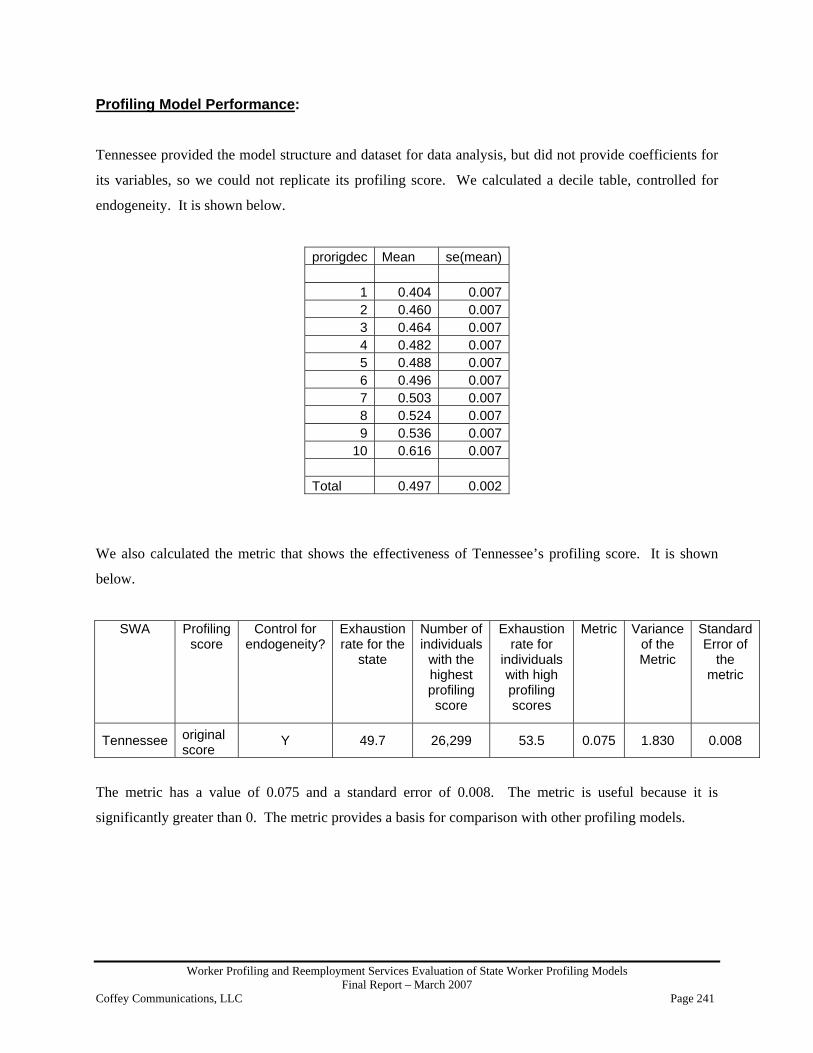
Worker Profiling and Reemployment Services Evaluation of State Worker Profiling Models Final Report – March 2007
Coffey Communications, LLC Page 241
Profiling Model Performance:
Tennessee provided the model structure and dataset for data analysis, but did not provide coefficients for
its variables, so we could not replicate its profiling score. We calculated a decile table, controlled for
endogeneity. It is shown below.
prorigdec Mean se(mean)
1 0.404 0.0072 0.460 0.0073 0.464 0.0074 0.482 0.0075 0.488 0.0076 0.496 0.0077 0.503 0.0078 0.524 0.0079 0.536 0.007
10 0.616 0.007 Total 0.497 0.002
We also calculated the metric that shows the effectiveness of Tennessee’s profiling score. It is shown
below.
SWA Profiling score
Control for endogeneity?
Exhaustion rate for the
state
Number of individuals
with the highest profiling score
Exhaustion rate for
individuals with high profiling scores
Metric Variance of the Metric
Standard Error of
the metric
Tennessee original score
Y 49.7 26,299 53.5 0.075 1.830 0.008
The metric has a value of 0.075 and a standard error of 0.008. The metric is useful because it is
significantly greater than 0. The metric provides a basis for comparison with other profiling models.

Worker Profiling and Reemployment Services Evaluation of State Worker Profiling Models Final Report – March 2007
Coffey Communications, LLC Page 242
ANALYSIS OF TEXAS PROFILING MODEL
Introduction: Texas uses a statistical model, of which the functional form is logistic, to operate its WPRS Program.
The model is run weekly against the claimant first-payment file. The list of eligible candidates is
produced at that time and is refreshed automatically at the state level and made available to the Local
Workforce Development Boards (Boards) via the Rapid Reemployment Services (RRES) computer
system. The Boards may access their lists of candidates through a secure access system. The model was
both updated and revised in 2003 in coordination with RRES.
Data Collection Process: Initial claims are filed principally by telephone and Internet. They may also be filed by mail, but that
method is rarely used. All of the characteristics necessary to determine eligibility for WPRS are captured
at the time of the initial claim. The initial claims taker determines and assigns the claimant’s occupational
code using the SOC (Standard Occupational Classification) coding system. The primary employer of the
claimant is determined through a review of the tax database, and it is determined by whomever the
claimant names as the last employer (LEU) in the claim. There are a number of checks that verify the
accuracy of information that claimants provide when filing an initial claim, including:
• All claimants must provide their name, date of birth, sex and Social Security account number
when filing an Unemployment Insurance (UI) claim. This information is automatically cross-
matched with the Social Security Administration (SSA) records to verify that the information
provided by the claimant matches the SSA records. If a discrepancy is discovered through the
cross-match, an investigation will be initiated to determine the validity of the claim. A claimant
will not be paid benefits until the SSA verifies the accuracy of the information provided by the
claimant or the Texas Workforce Commission (TWC), or the claimant corrects errors in the
record.
• All claimants are asked to provide their Texas Driver’s License (TDL) or Texas Identification
(TID) number when filing an initial claim. The information is not required to file a claim, but if it
is provided, the name, date of birth and TDL or TID number are automatically cross-matched
with the Texas Department of Public Safety (DPS) records to verify the accuracy and authenticity
of the information provided by the claimant. TWC will initiate an investigation to determine the
validity of the identity of the claimant when the DPS cross-match indicates a discrepancy.

Worker Profiling and Reemployment Services Evaluation of State Worker Profiling Models Final Report – March 2007
Coffey Communications, LLC Page 243
• All individuals filing claims are asked if they are citizens of the United States (US). Individuals
who are not citizens are required to submit documentation from the Immigration and
Naturalization Service (INS) that they have entered the US legally for the purposes of
employment. The INS registration number provided by the non-citizen claimant is cross-matched
with INS records to verify its authenticity and the claimants’ legal status to work in the US. Any
discrepancies in the INS registration number and/or records will initiate an investigation into the
accuracy of the information provided by the claimant and the validity of the claim.
• Claimants are required to provide a mailing address when filing an initial claim. The address
information is verified through a cross-match with the United States Postal Service (USPS)
records. The cross-match verifies that the address is a standardized or valid address according to
USPS records.
• Claimants list the name of the person or entity that they last worked for prior to filing the initial
claim. A notice of application for benefits is mailed to the LEU named by the claimant. The
notice to the employer includes the dates that the claimant worked and the reason for separation.
The employer has an opportunity to either confirm or dispute any employment information
provided by the claimant.
The following individuals are not eligible for WPRS services:
• Claimants who are not required to perform work search
• Claimants have union hall status
• Claimants have a definite return-to-work date
Selection/Referral Process: The list of WPRS eligible candidates is produced at the same time that the model is run against the first
payment file. The list is refreshed automatically at the state level and made available to the Local
Workforce Development Boards (Boards) via the RRES computer system. Boards have access to it
through a secure network. Each Board chooses the number of profiled candidates to be served based on
the capacity of the workforce centers. The model ranks individuals beginning with the highest to lowest
probabilities of exhaustion. Boards must select candidates with the highest score and work down the list
in descending order.

Worker Profiling and Reemployment Services Evaluation of State Worker Profiling Models Final Report – March 2007
Coffey Communications, LLC Page 244
Profiling Model Structure: Texas uses a statistical model, of which the functional form is logistic, to operate its WPRS Program.
The dependent variable is benefit exhaustion, defined as maximum benefits paid. The independent
variables are:
• Potential Duration of Benefits
• Job Tenure
• Delay in Filing
• Metroplex Economic Region
• Log of Weekly Benefit Amount
• Log of Average Weekly Wage
• COG-level Unemployment Rate
• Need for Public Transportation
• Industry Code
• Occupation Code
Profiling Model Performance:
Texas provided the model structure and dataset for data analysis. Our first step in analyzing both the
model used and the data was to order the provided profiling scores into a decile table as shown below.
The decile means (the average for each group representing 10 percent) in this table are calculated by
dividing the percentage of recipients that exhaust UI benefits for a given decile by 100. For example, in
the first decile our mean is 0.3120462, which indicates that approximately 31 percent of benefit recipients
in this decile exhausted benefits.
Decile Mean Standard Error (Mean) 1 .312 .00232652 .379 .00240183 .415 .00248954 .426 .00249065 .461 .00251326 .478 .00247867 .511 .00254928 .547 .00248349 .596 .002475310 .678 .0023531Total .480 .0007935

Worker Profiling and Reemployment Services Evaluation of State Worker Profiling Models Final Report – March 2007
Coffey Communications, LLC Page 245
After creating this decile table, we attempted to replicate these scores using the data and coefficients for
the variables given in the document “Rapid Reemployment Model.” We were able to identify all
variables from the dataset provided. However, there were two factors that limited our ability to replicate
the given profiling score. First, there was no constant provided with the model. To address this, through
trial and error of picking constant values, we estimated a constant for the model to be 0.2775. This
enabled us to replicate the profiling scores for most cases. Second, there were 433 cases, out of a sample
of 396,447, for which data were missing. Therefore, our analysis will be based on the 396,014 cases for
which we have complete information.
Even for the cases with complete information, our replication of the SWA profiling score was
significantly different from that which the SWA provided; there may be two reasons for this difference.
First, the given coefficients were rounded off to two or three significant digits. For a model with 19
variables, this rounding could, in some cases, make a large difference in the estimated profiling score.
However, there remained some cases with large differences. Second, there may be cases for which data
were not accurate. Therefore, we assume that some individuals may have inaccurate information for at
least one variable.
Texas included a binary variable indicating whether or not benefit recipients were referred to
reemployment services; therefore, we were able to test for endogeneity within the data regarding whether
referral to reemployment services had an effect on the exhaustion of benefits. We proceed with the
assumption that the given profiling score is what Texas used in its WPRS referral system for 2003.
By adjusting our original scores with a control variable for endogeneity, we estimated the true exhaustion
rate for the original score. Taking the predictions of the model, ordering them and dividing into deciles,
and then for each decile, showing the actual exhaustion rate, with its standard error, we obtain the
following table. This decile table demonstrates the effectiveness of each model.
Decile Mean Standard Error (Mean) 1 .312 .00232352 .378 .00242863 .416 .00245534 .426 .00251165 .461 .00250316 .479 .00249437 .51 .0025307

Worker Profiling and Reemployment Services Evaluation of State Worker Profiling Models Final Report – March 2007
Coffey Communications, LLC Page 246
8 .546 .00249189 .597 .002468310 .677 .0023529 Total .48 .0007935 The decile means are calculated by dividing the percentage of recipients that exhaust benefits for a given
decile by 100. For example, in the first decile our mean is 0.312, which indicates that approximately 31
percent of benefit recipients in this decile exhausted benefits.
Using the dataset provided, we continued our analysis of Texas’ profiling model by creating three models
– an updated, a revised, and a Tobit model. For each of the models, new profiling scores were created,
ranked, and divided into deciles. The table below shows the decile gradient for each of our models
(detailing the mean for each decile) and includes the decile gradient for the original model for reference.
From the table, we see that there was no improvement between the original and updated models in terms
of decile gradient changes.
Decile Original
Score Original score (Adjusted for Endogeneity)
Updated score Revised score Tobit score
1 .312 .312 .316 .308 .3122 .379 .378 .374 .367 .373 .415 .416 .406 .404 .4054 .426 .426 .435 .434 .4345 .461 .461 .456 .463 .4636 .478 .479 .482 .486 .4847 .511 .51 .513 .513 .5098 .547 .546 .543 .542 .5429 .596 .597 .597 .598 .59510 .678 .677 .676 .682 .685 Total .48 .48 .48 .48 .48 In addition, we tested the performance of each model using the following metric:
Percent exhausted of the top 48 percent of individuals in the score.
We used 48 percent because the exhaustion rate for benefit recipients in the dataset provided by Texas
was 48 percent. This metric value will vary from about 48 percent, for a score that is a random draw, up

Worker Profiling and Reemployment Services Evaluation of State Worker Profiling Models Final Report – March 2007
Coffey Communications, LLC Page 247
to 100 percent for a score that is a perfect predictor of exhaustion. The scores for the four models are as
follows:
Score % exhausted of those with the top 48% of score Standard error of the score Original 56.57 0.0011353 Updated 56.65 0.001136 Revised 56.87 0.0011353 TOBIT 56.73 0.0011357 In the metric below, “Exhaustion” is the percentage of all benefit recipients in our sample that exhaust
benefits. For Texas, “Exhaustion” is 48 percent since the exhaustion rate for all benefit recipients in the
dataset was 48 percent. In our metric, “Pr[Exh]” is determined by the model with the highest percentage
of benefit exhaustees with profiling scores falling in the top X percent of the sample, where X percent is
determined by the exhaustion rate for all benefit recipients in the sample. For Texas, “Pr[Exh]” is
represented by the revised model with a score of 56.87 percent for benefit recipients that exhaust benefits
with scores falling in the top 48 percent.
100 – Pr[Exh] Metric: 1 – 100 – Exhaustion We used the numbers above to calculate a score of 0.165 for the original profiling score (corrected for
endogeneity) and a score of 0.170 for the revised score.
SWA Profiling
score Control for
endogeneity? Exhaustion rate for the
state
Number of individuals
with the highest profiling score
Exhaustion rate for
individuals with high profiling scores
Metric Variance of the Metric
Standard Error of
the metric
Texas original score
Y 48.0 190,270 56.6 0.165 1.555 0.003
Texas revised score
Y 48.0 190,270 56.9 0.170 1.545 0.003
These metrics show that the revised model is significantly better that the original score. The metrics also
show a baseline on which other models can improve. Further analysis of Texas’ model is in the expanded
analysis section.

Worker Profiling and Reemployment Services Evaluation of State Worker Profiling Models Final Report – March 2007
Coffey Communications, LLC Page 248
ANALYSIS OF UTAH PROFILING MODEL
Introduction: Utah uses a statistical model, of which the functional form is logistic, to determine a claimant’s Worker
Profiling and Reemployment Services (WPRS) profiling score. The model is run weekly against the
claimant first payment records, and a list of WPRS eligible claimants is produced and sent to a UI
Specialist in the Administrative Office through the web-based reporting tool called “Actuate.” This list
ranks candidates in order from highest probabilities of exhaustion to lowest, and claimants are selected for
services by their probability score compared to other claimants in the same geographical region. The
number of candidates selected to be served is determined by the Unemployment Insurance (UI) Director
based on the number of Employment Counselors in the local office so that they each receive six per year.
A revised model was implemented in April 2004. It has not been updated since then. It replaced an
“antiquated” method of referring claimants for UI profiling services. The number of claimants included
in the sample for the latest revision is not available. When the model was first estimated, 46,644 benefit
recipients were included in the sample. Senior staff in Utah worked with Scott Gibbons in the ETA
National Office to develop a logistic regression model that calculates an exhaustion formula based on
several customer characteristics. The data warehouse sorts claimants within the program to identify 40
claimants most likely to exhaust benefits.
Data Collection Process:
Initial claims are filed by telephone and via the Internet. All of the claimant characteristics essential to
determine an individual’s eligibility for WPRS services are captured at the time of the initial claim. The
UI automated system checks the accuracy of the claimant’s name, date of birth, Social Security account
number and wages. The occupational code is assigned by the initial claims taker using the Standard
Occupational Classification (SOC) classification system. The industry code is based on a review of wage
records. Individuals not eligible for WPRS services include:
• Claimants who have a potential duration of less than 20 weeks
• Claimants who are union attached
• Claimants who are in recall status
• Claimants who are non-Utah residents
• Claimants who have filed additional or reopened claims

Worker Profiling and Reemployment Services Evaluation of State Worker Profiling Models Final Report – March 2007
Coffey Communications, LLC Page 249
Profiling Model Structure: The WPRS profiling model employed by the Utah utilizes a statistical model, of which the functional
form is logistic, to estimate benefit exhaustion. The dependent variable is exhaustion of benefits, defined
as claimants who have received their maximum benefits. Independent variables were selected based
principally on statistical significance. There were several possible variables that were examined that
proved less significant to the model, and they were dropped from consideration. Variables that were
selected include:
• Education
• Job Tenure
• Wage Replacement Rate
• High Quarter Earnings Rate
• Claim Filing Time Lapse (delay)
• Industry
• Severance Status
• Month of Filing
Profiling Model Performance: Utah did not provide a dataset for data analysis and/or model revision; therefore, we were unable to gauge
the performance of Utah’s current model.

Worker Profiling and Reemployment Services Evaluation of State Worker Profiling Models Final Report – March 2007
Coffey Communications, LLC Page 250
ANALYSIS OF VERMONT PROFILING MODEL
Introduction: Vermont uses a statistical model, of which the functional form is logistic, to determine a claimant’s
Worker Profiling and Reemployment Services (WPRS) profiling score. The model is run weekly against
the claimant first payment file, and the list of eligible candidates is distributed to the Job Service Offices
in hard copy. This list ranks candidates in order from highest to lowest probabilities of exhaustion. The
Job Service District Office determines the number to be served, and it cannot skip individuals with higher
scores to service those with lower scores.
The model was last revised in March 2005. At that time, the occupational classification system in use
was changed to the Standard Occupational Classification (SOC) system and the Weekly Benefit Amount
(WBA) was removed as a variable. Initial claimants totaling 27,087 were used as the sample in the
revision. In the revision of the model in 2001, 11,291 initial claims filers were included in the sample.
Data Collection Process:
All initial claims are filed by telephone. Claimant characteristics necessary to determine an individual’s
eligibility for WPRS services are obtained by the initial claims taker who also determines and assigns the
occupational code using the SOC classification system. The industry code is obtained from the tax data
base. Claimants with a return to work date are not eligible for referral to WPRS services.
Selection/Referral Process:
The WPRS model is run against the claimant first payment file and a list of eligible candidates is
produced at that time. Claimants are listed by probability of exhaustion. The list is distributed in hard
copy to the Job Service Offices. The Job Service District Office determines the number to be served.
Local Office Staff cannot skip individuals with higher scores to service those with lower ones.

Worker Profiling and Reemployment Services Evaluation of State Worker Profiling Models Final Report – March 2007
Coffey Communications, LLC Page 251
Profiling Model Structure:
The WPRS profiling model employed by Vermont utilizes a statistical model, of which the functional
form is logistic, to estimate benefit exhaustion. The dependent variable is exhaustion of benefits, defined
as maximum benefits paid. The independent variables are as follows:
• Claimant Previously Profiled
• Number of Lag Weeks Since Filing of Initial Claim
• Job Tenure
• Education
• SOC Classification
• Industry Code
• High Quarter Wages
Profiling Model Performance:
Vermont provided the model structure and dataset for data analysis but did not provide coefficients for the
variables in its profiling model, so we could not replicate its profiling score. Vermont provided data on
referral to reemployment services, but its effect was not significant. We did not control for endogeneity.
We calculated a decile table for the original score. It is shown below.
prorigdec Mean se(mean)
1 0.219 0.0372 0.172 0.0333 0.277 0.0394 0.252 0.0385 0.258 0.0396 0.228 0.0377 0.326 0.0418 0.258 0.0399 0.392 0.044
10 0.457 0.044 Total 0.283 0.013
We also calculated the metric that shows the effectiveness of Vermont’s profiling score. It is shown
below.
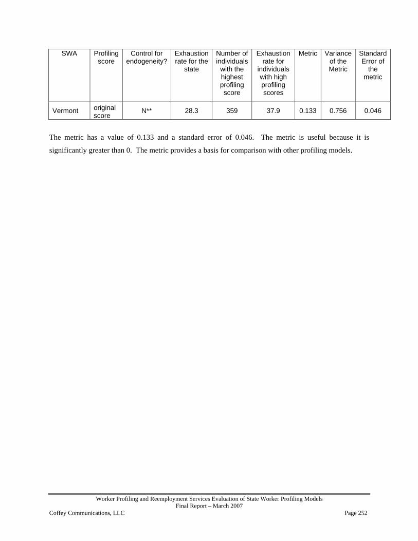
Worker Profiling and Reemployment Services Evaluation of State Worker Profiling Models Final Report – March 2007
Coffey Communications, LLC Page 252
SWA Profiling score
Control for endogeneity?
Exhaustion rate for the
state
Number of individuals
with the highest profiling score
Exhaustion rate for
individuals with high profiling scores
Metric Variance of the Metric
Standard Error of
the metric
Vermont original score
N** 28.3 359 37.9 0.133 0.756 0.046
The metric has a value of 0.133 and a standard error of 0.046. The metric is useful because it is
significantly greater than 0. The metric provides a basis for comparison with other profiling models.

Worker Profiling and Reemployment Services Evaluation of State Worker Profiling Models Final Report – March 2007
Coffey Communications, LLC Page 253
ANALYSIS OF VIRGINIA PROFILING MODEL
Introduction: Virginia uses a statistical model, of which the functional form is logistic, to determine a claimant’s
Worker Profiling and Reemployment Services (WPRS) profiling score. The model is run weekly against
the claimant first payment records, and a list of WPRS eligible claimants is sent to local offices via
mainframe screens. This list ranks candidates in order from highest probabilities of exhaustion to lowest.
All claimants, regardless of probabilities of exhaustion, are shown on the list along with their rankings.
In certain cases, local office staff may select candidates with lower rankings who have been posted in the
pool for four weeks (they will drop off the list if they are not selected for services). These candidates may
be selected before candidates with higher rankings who have just entered the pool and will likely remain
in the pool long enough to be called in for services.
The model is currently undergoing its first revision since its inception. It has not been updated to
generate new statistical parameters. However, tables containing the explanatory variables of
unemployment rate by Service Delivery Area (SDA) and industry growth or decline are updated as
Virginia’s Economic Information System deems appropriate.
Data Collection Process:
Initial claims are filed in-person, by telephone and by Internet. The initial claims taker assigns the
claimant’s occupational code using the DOT (Dictionary of Occupational Titles) classification system
unless the claim is filed on the Internet. In that case, the claimant self-selects his/her occupational code
based on a pop-up list of codes. The industry code is also assigned by claims takers using the SIC
(Standard Industrial Classification) system. Previous job position, length of time employed salary, etc.,
are verified with the employer by use of a “separation statement.” Individuals not eligible for referral to
WPRS services include:
• Claimants with specific recall dates
• Claimants with union hiring agreements
• Claimants not residing in Virginia

Worker Profiling and Reemployment Services Evaluation of State Worker Profiling Models Final Report – March 2007
Coffey Communications, LLC Page 254
Selection/Referral Process:
The WPRS model is run weekly against the claimant first payment file, and a list of eligible candidates is
produced at that time. The list is organized by local office and made available via mainframe screen to all
local offices and the central office. Each local office determines the number of claimants that can be
served in that office with the gateway service of RSO. While each office strives to serve all eligible
candidates, the number of candidates notified depends on the availability of staff and facility resources.
Regional coordinators review this activity monthly and quarterly. Claimants with the highest rankings
(most likely to exhaust benefits) are selected first. Those with rankings beneath the minimum selection
threshold are shown on the list along with their rankings, but they are not part of the pool and thus are not
selected for WPRS services. In certain cases, local office staff may select candidates with lower rankings
who have been posted in the pool for four weeks and will drop off the list if they are not selected for
RSO.
Profiling Model Structure: The WPRS profiling model employed by Virginia utilizes a statistical model, of which the functional
form is logistic, to estimate benefit exhaustion. The dependent variable is benefit exhaustion, defined as
maximum benefits paid. The independent variables are as follows:
• Job Tenure (continuous)
• Education
• Occupation
• Unemployment Rate in Local Area
• Industry Growth at the Division Level in the Local Area
Profiling Model Performance:
Virginia provided the model structure and dataset for data analysis but did not provide variables for local
unemployment rate and local industry growth, so we could not replicate its profiling score. We calculated
a decile table for the original score, controlled for endogeneity. It is shown below.

Worker Profiling and Reemployment Services Evaluation of State Worker Profiling Models Final Report – March 2007
Coffey Communications, LLC Page 255
prorigdec Mean se(mean)
1 0.146 0.0042 0.180 0.0043 0.243 0.0054 0.242 0.0055 0.240 0.0046 0.236 0.0047 0.243 0.0058 0.249 0.0059 0.217 0.004
10 0.340 0.005 Total 0.233 0.001
We also calculated the metric that shows the effectiveness of Virginia’s profiling score. It is shown
below.
SWA Profiling score
Control for endogeneity?
Exhaustion rate for the
state
Number of individuals
with the highest profiling score
Exhaustion rate for
individuals with high profiling scores
Metric Variance of the Metric
Standard Error of
the metric
Virginia original score
Y 23.3 21,186 27.7 0.057 0.611 0.005
The metric has a value of 0.057 and a standard error of 0.005. The metric is useful because it is
significantly greater than 0. The metric provides a basis for comparison with other profiling models.

Worker Profiling and Reemployment Services Evaluation of State Worker Profiling Models Final Report – March 2007
Coffey Communications, LLC Page 256
ANALYSIS OF THE VIRGIN ISLANDS PROFILING MODEL
Introduction:
The Virgin Islands uses characteristic screening to determine a claimant’s eligibility for referral to
Worker Profiling and Reemployment Services (WPRS). The model is run weekly against the claimant
first payment file. First payment claimants are added to a pool of potential profiling candidates on a daily
basis. Claimants with the highest probability of exhaustion of benefits are selected for services first. The
model has never been updated or revised.
Data Collection Process:
All initial claims are filed in-person. Claimant characteristics essential to determine an individual’s
eligibility to participate in WPRS services is captured at the initial claim. Individuals must produce
suitable identification. A separation notice is obtained from the employer, and the initial claim is checked
for accuracy to verify the information provided by the claimant. The occupational code using the
Standard Occupational Classification (SOC) system is assigned by a Workforce Development Worker.
The claimant’s primary employer is assigned based on a review of the claimant’s work history. The
following individuals are not eligible for participation in WPRS services:
• Job Attached Claimant
• Interstate Claimants
• Claimants on Definite Recall
Selection/Referral Process:
Claimants are selected for participation in the WPRS program when the weekly first payment file is
matched with eligible claimants who are added to the pool daily. Claimants with the highest probability
of exhaustion must be selected for participation first. The only exception occurs in cases where there may
be unresolved non-monetary issues. The UI Service determines the number of candidates to be served by
the Reemployment Service based on a Memorandum of Understanding (MOU) between the two services.

Worker Profiling and Reemployment Services Evaluation of State Worker Profiling Models Final Report – March 2007
Coffey Communications, LLC Page 257
Profiling Model Structure:
The WPRS profiling model employed by the Virgin Islands utilizes a characteristic screen model to
estimate benefit exhaustion. This characteristic screen eliminates all claimants that are ineligible for
referral to reemployment services. The characteristics used to select candidates include:
• Education
• Job Tenure
• Occupation or Industry
Profiling Model Performance:
The Virgin Islands did not provide a dataset for data analysis and/or model revision; therefore, we were
unable to gauge the performance of The Virgin Islands’ current model.

Worker Profiling and Reemployment Services Evaluation of State Worker Profiling Models Final Report – March 2007
Coffey Communications, LLC Page 258
ANALYSIS OF WASHINGTON PROFILING MODEL
Introduction: Washington State uses a statistical model, of which the functional form is logistic, to determine a
claimant’s Worker Profiling and Reemployment Services (WPRS) profiling score. The model is run
weekly against the claimant first payment records, and a list of WPRS-eligible claimants is produced and
sent to the WorkSource One-Stop Offices using an electronic transfer from GUIDE (General
Unemployment Insurance Development Effort) to SKIES (Services, Knowledge and Information
Exchange System), which is Washington’s One-Stop case management system. This list ranks candidates
in order from highest to lowest probabilities of exhaustion, and each WorkSource office determines the
number of candidates to be selected. Claimants who have received and/or are participating in the same or
similar services are exempt from participation, as are those who have returned to work date or expectation
of recall.
The model was last revised in July, 2004. The SWA would like to revise the model annually; however,
resources may not always be available to make the revisions. All initial claims filers were included in the
most recent model revision sample. This was equal to 321,925 (80 percent) of the initial claims.
Data Collection Process:
Initial claims are filed in-person, by mail, by telephone and via the Internet. Claimant characteristics
essential to determine a claimant’s eligibility for WPRS are captured at the time the initial claim is filed.
Most of the characteristics are obtained from the GUIDE system, thus ensuring greater accuracy of the
data. The Dictionary of Occupational Titles (DOT) system, with a crosswalk to O*Net, is used as the
occupational classification system. The initial claims taker assigns the occupational code. The following
individuals are not eligible to participate in the WPRS Program:
• Claimants who are partially unemployed
• Claimants who are participating in the Shared Work Program
• Claimants on standby
• Claimants who are on full referral to jobs through a union
• Claimants participating in Commissioner Approved Training (CAT)
• Claimants who are on Total Temporary Disability

Worker Profiling and Reemployment Services Evaluation of State Worker Profiling Models Final Report – March 2007
Coffey Communications, LLC Page 259
Profiling Model Structure:
The WPRS profiling model employed by Washington utilizes a statistical model, of which the functional
form is logistic, to estimate benefit exhaustion. The dependent variable is benefit exhaustion, defined as
maximum benefits paid. Independent variables were not identified.
Profiling Model Performance: Washington State did not provide a dataset for data analysis and/or model revision; therefore, we were
unable to gauge the performance of Washington’s current model.

Worker Profiling and Reemployment Services Evaluation of State Worker Profiling Models Final Report – March 2007
Coffey Communications, LLC Page 260
ANALYSIS OF WEST VIRGINIA PROFILING MODEL
Introduction:
West Virginia uses a statistical model, of which the functional form is logistic, to determine a claimant’s
Worker Profiling and Reemployment Services (WPRS) profiling score. The model is run weekly against
the claimant first payment file and candidates are selected and placed on a list for participation at that
time. The list is sent to staff in the Administrative Office who have oversight responsibility for the
WPRS Program and Local Office staff who receive a paper report listing the claimants selected for
participation, including the date of their scheduled interview, etc.
During the third quarter of 2001, a new profiling model was implemented. The prior model used six
independent variables but consisted of several individual models. The model now in use has 10
predictive variables that have been condensed into one model. In this revision, a sample of 69,612 benefit
recipients was used. Two-thirds of the benefit recipients were used to build the model and the other one-
third was used to test and verify the outcomes. In conducting the revision, in addition to analyzing
historical independent variables, other potential ones, including Workforce Investment Act (WIA) regions
and wage replacement rates, were also reviewed and analyzed.
Data Collection Process:
Initial claims are taken in-person. Claimant characteristics necessary to determine an individual’s
eligibility for WPRS services are obtained during the initial claims taking process. Several of the
characteristics provided by the claimant are able to be checked for accuracy, including:
• Social Security numbers (SSN) through a crossmatch with the Social Security Administration
• North American Industry Classification System (NAICS) code through a check with the UI Wage
Record System
• Also, several of the characteristics must be entered in order for the claim to be posted to the UI
System.
The initial claims taker assigns the individual’s occupational code using the Standard Occupational
Classification (SOC) system classification system. The NAICS classification system is used to determine
the claimant’s proper industry, and it is based on an interview with the individual and a review of the UI
Wage Records. The following individuals are not eligible for referral to WPRS services:
• Claimants who obtain work through a union hiring hall.

Worker Profiling and Reemployment Services Evaluation of State Worker Profiling Models Final Report – March 2007
Coffey Communications, LLC Page 261
• Claimants who have a definite recall date
• Claimants who have been selected and offered a Personal Reemployment Account (PRA)
• Claimants who have a partial claim
• Claimants who have been profiled within the last 270 days
Selection/Referral Process:
At the same time that the WPRS model was being revised, it was decided that Job Service offices will use
the Resource Allocation method when scheduling claimants for profiling services. This serves a two-fold
purpose. First, the 50 percent exhaustion probability threshold has been eliminated which allows
everyone scored to be placed in the pool. Secondly, this requires each office to specify the number of
candidates to be served each week.
The profiled list is provided on a paper report showing the claimants who were selected along with their
interview date, etc. These reports are usually printed automatically in each local office, but if necessary,
they can be printed in the central office. Claimants are ranked by probability of exhaustion, and they are
selected in that order automatically – staff cannot bypass individuals on the list. Job Service Offices
determine the number of candidates to be called-in each week, based on workload and capacity and input
the number into the automated system.
Profiling Model Structure:
West Virginia uses a statistical model, of which the functional form is logistic, to estimate benefit
exhaustion. The dependent variable is benefit exhaustion, defined as maximum benefits paid. The
independent variables include:
• Weekly benefit amount
• Wage base*
• Tenure
• Reopens*
• SOC – 3 digit (formerly occupation with former employer)
• NAICS – 3 digit (formerly industry of former employer)
• Education
• Benefit Year Begin Month (old model had only January seasonal factor)

Worker Profiling and Reemployment Services Evaluation of State Worker Profiling Models Final Report – March 2007
Coffey Communications, LLC Page 262
• File lag*
• Other income*
* - New variables in the 2001 model
Profiling Model Performance:
West Virginia provided the model structure and dataset for data analysis. Our first step in analyzing both
the model used and the data was to order the provided profiling scores into a decile table as shown below.
The decile means (the average for each group representing 10 percent) in this table are calculated by
dividing the percentage of recipients that exhaust UI benefits for a given decile by 100. For example, in
the first decile our mean is 0.2116, which indicates that approximately 21 percent of benefit recipients in
this decile exhausted benefits.
Decile Mean Standard Error (Mean) 1 .2116266 .0069132 2 .2552277 .0073801 3 .3091898 .0078209 4 .3562428 .0081051 5 .37611 .0081997 6 .4039508 .0083036 7 .4428531 .0084082 8 .4696101 .0084516 9 .4801031 .0084545 10 .5611923 .0084024 Total .3865895 .0026062
After creating this decile table, we replicated the original profiling scores. We were able to identify all
variables from the dataset provided. Our replicated SWA profiling score was correlated with the original
score at 0.9277.
West Virginia included a binary variable indicating whether or not benefit recipients were referred to
reemployment services; therefore, we were able to test for endogeneity within the data regarding whether
referral to reemployment services had an effect on the exhaustion of benefits.
By adjusting our original scores with a control variable for endogeneity, we estimated the true exhaustion
rate for the original score. Taking the predictions of the model, ordering them and dividing into deciles,

Worker Profiling and Reemployment Services Evaluation of State Worker Profiling Models Final Report – March 2007
Coffey Communications, LLC Page 263
and then for each decile, showing the actual exhaustion rate, with its standard error, we obtain the
following table. This decile table demonstrates the effectiveness of each model.
Decile, original score corrected for endogeneity
Mean Standard Error (Mean)
1 .2124857 .0069234 2 .25666 .0073937 3 .3070979 .007805 4 .3553009 .0081026 5 .382235 .0082267 6 .3981667 .0082862 7 .4372852 .0083956 8 .4743626 .0084525 9 .4800917 .0084569 10 .5623031 .0083977 Total .3865895 .0026062 We continued our analysis of West Virginia’s profiling model by creating two models – an updated and a
revised model. We could not create a Tobit model because there was no way to calculate the proportion
of benefits remaining in individuals’ UI benefit accounts. For each of the models, new profiling scores
were created, ranked, and divided into deciles. The table below shows the decile gradient for each of our
models (detailing the mean for each decile) and includes the decile gradient for the original model for
reference. From the table, we see that there was significant improvement between the original and
updated models but no improvement for the revised model.
Decile Original
Score Original score (Adjusted for Endogeneity)
Updated score Revised score
1 .2160804 .2135395 .175957 .1796508 2 .2632411 .2686275 .2437878 .259906 3 .3236351 .3225689 .2971793 .3270651 4 .3774373 .3756047 .3399395 .3557272 5 .3924802 .3968833 .3895232 .3841504 6 .4150641 .4106452 .4308261 .4378778 7 .4629278 .4558684 .4662412 .4685925 8 .4799627 .4879032 .5238415 .5063801 9 .4918478 .4909475 .5815984 .5503694 10 .5734245 .5737608 .6536782 .6328519 Total .4102495 .4102495 .4102495 .4102495

Worker Profiling and Reemployment Services Evaluation of State Worker Profiling Models Final Report – March 2007
Coffey Communications, LLC Page 264
In addition, we tested the performance of each model using the following metric:
Percent exhausted of the top 41 percent of individuals in the score. We used 41 percent because the exhaustion rate for benefit recipients in the dataset provided by West
Virginia was 41 percent. This metric value will vary from about 41 percent, for a score that is a random
draw, up to 100 percent for a score that is a perfect predictor of exhaustion. The scores for the four
models are as follows:
Score % exhausted of those with the top 41% of score Standard error of the score
Original .50692 .0045245 Adapted .5070042 .0045252 Updated .5536899 .0044991 Revised .5373904 .0045126 In the metric below, “Exhaustion” is the percentage of all benefit recipients in our sample that exhaust
benefits. For West Virginia, “Exhaustion” is 41 percent since the exhaustion rate for all benefit recipients
in the dataset was 41 percent. In our metric, “Pr[Exh]” is determined by the model with the highest
percentage of benefit exhaustees with profiling scores falling in the top X percent of the sample, where X
pecent is determined by the exhaustion rate for all benefit recipients in the sample. For West Virginia,
“Pr[Exh]” is represented by the updated model with a score of 55.37 percent for benefit recipients that
exhaust benefits with scores falling in the top 41 percent.
100 – Pr[Exh] Metric: 1 – 100 – Exhaustion We used the numbers above to calculate a score of 0.164 for the original profiling score (corrected for
endogeneity) and a score of 0.243 for the updated score.
SWA Profiling
score Control for
endogeneity? Exhaustion rate for the
state
Number of individuals
with the highest profiling score
Exhaustion rate for
individuals with high profiling scores
Metric Variance of the Metric
Standard Error of
the metric
West Virginia
original score
Y 41.0 12,209 50.7 0.164 1.205 0.010
West Virginia
updated score
Y 41.0 12,209 55.4 0.243 1.109 0.010
These metrics show that the updated model is significantly better that the original score. The metrics also
show a baseline on which other models can improve. Further analysis of West Virginia’s model is in the
expanded analysis section.

Worker Profiling and Reemployment Services Evaluation of State Worker Profiling Models Final Report – March 2007
Coffey Communications, LLC Page 265
ANALYSIS OF WISCONSIN PROFILING MODEL
Introduction:
Wisconsin uses a statistical model, of which the functional form is logistic, to determine a claimant’s
Worker Profiling and Reemployment Services (WPRS) profiling score. The model is run weekly against
the claimant first payment file with selection for participation made centrally when requested by local
centers. The resulting list ranks candidates in order from highest to lowest probabilities of exhaustion and
local areas have no input or influence in the selection. The model has never been updated or revised. It
has been in use since 1994, when WPRS was initiated.
Data Collection Process:
Initial claims are filed by telephone and Internet. Claimant characteristics necessary to determine an
individual’s eligibility for WPRS services are obtained during the initial claims taking process. Student
status, union hiring hall (in good standing), and early recall with an employer are verified. The initial
claims taker determines the occupational code using the Standard Occupational Classification (SOC)
system. A review of UI wage records is performed to determine the industry classification. The
following individuals are not eligible for participation in WPRS services:
• Union hiring hall
• Student status
• Partially employed
• Recall pending
Selection/Referral Process:
Individuals are determined eligible for WPRS services when the model is run weekly against the claimant
first payment file. Selection is made centrally by profiling score in the One-Stop site ZIP code area. The
only decision local staff can make is the number and frequency of group sessions that can be
accommodated. This is principally determined by staff and facility availability.

Worker Profiling and Reemployment Services Evaluation of State Worker Profiling Models Final Report – March 2007
Coffey Communications, LLC Page 266
Profiling Model Structure:
The WPRS profiling model employed by Wisconsin utilizes a statistical model, of which the functional
form is logistic, to estimate benefit exhaustion. The dependent variable is benefit exhaustion, defined as
maximum benefits paid. The independent variables are as follows:
• Tenure with Primary Employer
• Total Unemployment Rate in County
• Occupation
• Education
• Industry
Profiling Model Performance:
Wisconsin provided the model structure and dataset for data analysis but did not provide coefficients for
the variables used in their model, so we could not replicate its profiling score. Wisconsin did not provide
a variable for referral to reemployment services, so we could not control for endogeneity. We calculated
a decile table for the original score. It is shown below.
prorigdec Mean se(mean)
1 0.375 0.0112 0.422 0.0113 0.433 0.0114 0.437 0.0115 0.457 0.0116 0.446 0.0117 0.473 0.0118 0.508 0.0119 0.434 0.008
Total 0.442 0.003
Note that there were some individuals with the same profiling score, so we were not able to generate 10
separate categories. We also calculated the metric that shows the effectiveness of Wisconsin’s profiling
score. It is shown below.

Worker Profiling and Reemployment Services Evaluation of State Worker Profiling Models Final Report – March 2007
Coffey Communications, LLC Page 267
SWA Profiling score
Control for endogeneity?
Exhaustion rate for the
state
Number of individuals
with the highest profiling score
Exhaustion rate for
individuals with high profiling scores
Metric Variance of the Metric
Standard Error of
the metric
Wisconsin original score
N 44.2 8,991 46.2 0.036 1.533 0.013
The metric has a value of 0.036 and a standard error of 0.013. The metric is useful because it is
significantly greater than 0. The metric provides a basis for comparison with other profiling models.

Worker Profiling and Reemployment Services Evaluation of State Worker Profiling Models Final Report – March 2007
Coffey Communications, LLC Page 268
ANALYSIS OF WYOMING PROFILING MODEL
Summary:
Wyoming uses a statistical model with a discriminant analysis functional form to select individuals for
participation in the WPRS Program. The model is run weekly against the initial claim file, and a list of
eligible candidates is produced at that time. The list is then sent to the profiling coordinator in the SWA
claims center for review and distribution to the local offices. The model is revised every two or three
years. As part of the 2001 revision, the logistic regression previously used was changed to a discriminant
analysis statistical model. In July, 2005, the most recent update occurred when the coefficients were
updated with more current database information to reflect current economic conditions.
Data Collection Process:
Initial claims are filed in-person, by telephone, by mail, and by Internet. The most prevalent method is
telephone filing with 82 percent of the claimants using it. Claimant characteristics are captured at the
time the initial claim is taken. The initial claims taker assigns the occupational code using the SOC
classification system. The primary employer is determined based on information provided by the
claimant and then verified through the wage record system. Additional checks on the accuracy of
information provided by the claimant are done through a crossmatch with the Social Security
Administration. Following a notification to the employer that a former employee has filed a claim,
Benefit Accuracy Measurement (BAM) reviews, and benefit payment control crossmatch. The following
individuals are not eligible for referral to WPRS services:
• The claimant is a member of a union or hiring hall or is job attached
• The claimant is filing an interstate claim which is not Wyoming liable
• The claimant worked for his/her last employer for less than 52 weeks
• The claimant is filing a continued or additional claim
• The claimant with any of the variables requested by the model equals zero
Selection/Referral Process:
Candidates for referral to WPRS services are selected weekly when the model is run against the initial
claims payment file. A list of individual candidates is provided to the profiling coordinator in the SWA
claims center who reviews it prior to distributing it to local offices. In the review, the coordinator may

Worker Profiling and Reemployment Services Evaluation of State Worker Profiling Models Final Report – March 2007
Coffey Communications, LLC Page 269
exclude and delete from the list, the following claimants:
• Individuals who have received similar services
• Individuals who have returned to work
• Individuals who have moved out of state
• Individuals who are monetarily not eligible or not likely to become eligible
The list is arrayed by probability of exhaustion ranked from highest to lowest. Claimants are included in
the pool when their probability of exhaustion equals or exceeds 60 percent.
Profiling Model Structure:
The WPRS profiling model employed by Wyoming utilizes a statistical model with a discriminant
analysis functional form to estimate benefit exhaustion. The dependent variable is benefit exhaustion,
which is determined by a final payment indicator flag that is set for the initial claimant. The independent
variables are as follows:
• Natural Log of Job Tenure
• Natural Log of Delay in Filing
• Number of Employers
• Weeks Eligible for Benefits
• Unemployment Rate for Industry
• Whether Claimant was Employed in a Declining Industry
• Month Claim is Filed
• NAICS Industry Code
• Total Unemployment Rate in County
Profiling Model Performance:
Wyoming provided the model structure and dataset for data analysis. We were able to replicate the
original profiling score, but the sample size was too small (N=107) to merit further analysis. Wyoming
did provide a variable for referral to reemployment services, but its effect was insignificant. There was
no need to control for endogeneity. We calculated a decile table for the original score. It is shown below.

Worker Profiling and Reemployment Services Evaluation of State Worker Profiling Models Final Report – March 2007
Coffey Communications, LLC Page 270
prorigdec N mean se(mean) 1 8 0.500 0.189 2 12 0.333 0.142 3 10 0.300 0.153 4 10 0.500 0.167 5 14 0.500 0.139 6 8 0.375 0.183 7 12 0.500 0.151 8 9 0.667 0.167 9 11 0.273 0.141
10 13 0.462 0.144
Total 107 0.439 0.048
We also calculated the metric that shows the effectiveness of Wyoming’s profiling score. It is shown
below.
SWA Profiling score
Control for endogeneity?
Exhaustion rate for the
state
Number of individuals
with the highest profiling score
Exhaustion rate for
individuals with high profiling scores
Metric Variance of the Metric
Standard Error of
the metric
Wyoming original score
N** 43.9 47 46.8 0.051 1.497 0.178
** SWA provided data indicating individuals who were referred, but the effect was insignificant.
The metric has a value of 0.051 and a standard error of 0.178. The metric is not useful because it is not
significantly greater than 0. The metric provides a basis for comparison with other profiling models. A
better model would generate a higher metric.

Worker Profiling and Reemployment Services Evaluation of State Worker Profiling Models Final Report – March 2007
Coffey Communications, LLC Page 271
APPENDIX D: EXPANDED ANALYSES FOR 9 SWAS

Worker Profiling and Reemployment Services Evaluation of State Worker Profiling Models Final Report – March 2007
Coffey Communications, LLC Page 272
In this section, we provide detailed analysis that includes all the elements described above in the
Chapter on extended data analysis. These analyses represent our best attempt to improve upon
the methodology for generating effective profiling scores.
We include here extended analyses for all SWAs for which we could replicate the given profiling
score and exhaustion status. That means the SWA provided data for all variables used in its
profiling score and all coefficients for variables, and that SWAs provided data on whether the
individuals exhausted benefits. There is one exception to this rule: Wyoming. Because
Wyoming only had 107 individuals with full information, there were not enough degrees of
freedom to conduct a useful analysis.
Included here are extended analyses for:
• Arkansas • District of Columbia • Georgia • Hawaii • Idaho • New Jersey • Pennsylvania • Texas • West Virginia
The analyses and statistics are described above. Our analyses minimize the text. They are very
table-intensive.

Worker Profiling and Reemployment Services Evaluation of State Worker Profiling Models Final Report – March 2007
Coffey Communications, LLC Page 273
Decile Tables for 28 SWAs
The Table below contains decile tables for 28 SWAs. The tables were formed by first ranking all
individuals in the sample by profiling score and then dividing the sample into 10 equal groups.
For each group, we calculated the mean rate of exhaustion of UI benefits for the group. The
tables include the standard error of each exhaustion rate. For most SWAs, the table includes
only the original score, and if possible, the score was corrected for endogeneity. For nine states
for which we conducted expanded analyses, we include two decile tables: one for the original
score and one for the best other score that we calculated – usually the revised model score.
Arizona prorigdec mean se(mean)
1 0.350 0.006 2 0.330 0.006 3 0.348 0.006 4 0.346 0.006 5 0.341 0.006 6 0.375 0.006 7 0.373 0.006 8 0.400 0.006 9 0.418 0.007
10 0.508 0.007 Total 0.379 0.002 Arkansas Original score Revised score scoredec mean se(mean) prrevdec mean se(mean)
1 0.379 0.007 1 0.326 0.006 2 0.462 0.007 2 0.414 0.007 3 0.467 0.007 3 0.426 0.007 4 0.484 0.007 4 0.471 0.007 5 0.472 0.007 5 0.477 0.007 6 0.491 0.007 6 0.503 0.007 7 0.496 0.007 7 0.535 0.007 8 0.522 0.007 8 0.552 0.007 9 0.577 0.007 9 0.606 0.007

Worker Profiling and Reemployment Services Evaluation of State Worker Profiling Models Final Report – March 2007
Coffey Communications, LLC Page 274
10 0.647 0.007 10 0.685 0.006 Total 0.499 0.002 Total 0.499 0.002 Delaware Estimated score predscoredec mean se(mean)
1 0.350 0.014 2 0.318 0.014 3 0.419 0.015 4 0.383 0.015 5 0.365 0.015 6 0.375 0.015 7 0.394 0.015 8 0.404 0.015 9 0.415 0.015
10 0.475 0.015 Total 0.390 0.005 District of Columbia Original score Revised score scoredec mean se(mean) prrevdec mean se(mean)
1 0.416 0.016 1.000 0.341 0.015
2 0.501 0.016 2.000 0.469 0.016
3 0.533 0.016 3.000 0.492 0.016
4 0.543 0.016 4.000 0.511 0.016
5 0.598 0.016 5.000 0.560 0.016
6 0.541 0.016 6.000 0.602 0.016
7 0.582 0.016 7.000 0.607 0.016
8 0.596 0.016 8.000 0.629 0.016
9 0.644 0.015 9.000 0.658 0.015
10 0.649 0.016 10.000 0.732 0.014
Total 0.560 0.005 Total 0.560 0.005

Worker Profiling and Reemployment Services Evaluation of State Worker Profiling Models Final Report – March 2007
Coffey Communications, LLC Page 275
Georgia Original score Revised score prorigdec mean se(mean) prrevdec mean se(mean)
1 0.269 0.003 1 0.175 0.003 2 0.319 0.003 2 0.233 0.003 3 0.313 0.003 3 0.276 0.003 4 0.294 0.004 4 0.309 0.003 5 0.286 0.003 5 0.345 0.003 6 0.336 0.003 6 0.374 0.003 7 0.336 0.003 7 0.402 0.003 8 0.404 0.004 8 0.438 0.004 9 0.487 0.004 9 0.499 0.004
10 0.526 0.004 10 0.518 0.004 Total 0.357 0.001 Total 0.357 0.001 Hawaii Original score Revised score prorigdec mean se(mean) prrevdec mean se(mean)
1 0.327 0.016 1 0.308 0.015 2 0.314 0.016 2 0.319 0.016 3 0.376 0.016 3 0.338 0.016 4 0.376 0.016 4 0.385 0.016 5 0.405 0.016 5 0.373 0.016 6 0.389 0.016 6 0.422 0.016 7 0.406 0.016 7 0.423 0.017 8 0.423 0.017 8 0.418 0.016 9 0.457 0.017 9 0.454 0.017
10 0.467 0.017 10 0.499 0.017 Total 0.394 0.005 Total 0.394 0.005 Idaho Estimated score Revised score prorigdec mean se(mean) prrevdec mean se(mean)
1 0.412 0.008 1 0.216 0.007 2 0.394 0.008 2 0.297 0.008 3 0.365 0.008 3 0.359 0.008

Worker Profiling and Reemployment Services Evaluation of State Worker Profiling Models Final Report – March 2007
Coffey Communications, LLC Page 276
4 0.360 0.008 4 0.392 0.008 5 0.350 0.008 5 0.425 0.008 6 0.362 0.008 6 0.459 0.009 7 0.439 0.009 7 0.500 0.009 8 0.550 0.009 8 0.566 0.009 9 0.650 0.008 9 0.642 0.008
10 0.710 0.008 10 0.734 0.008 Total 0.459 0.003 Total 0.459 0.003 Iowa prorigdec mean se(mean)
1 0.145 0.008 2 0.152 0.004 8 0.162 0.010 9 0.156 0.010
10 0.170 0.010 Total 0.154 0.003 Louisiana prorigdec mean se(mean)
1 0.325 0.006 2 0.322 0.006 3 0.341 0.006 4 0.383 0.007 5 0.407 0.007 6 0.383 0.007 7 0.477 0.007 8 0.500 0.007 9 0.505 0.007
10 0.621 0.007 Total 0.426 0.002 Maine prorigdec mean se(mean)
1 0.275 0.010 2 0.319 0.010 3 0.342 0.011

Worker Profiling and Reemployment Services Evaluation of State Worker Profiling Models Final Report – March 2007
Coffey Communications, LLC Page 277
4 0.353 0.011 5 0.368 0.011 6 0.390 0.011 7 0.387 0.011 8 0.382 0.011 9 0.416 0.011
10 0.503 0.011 Total 0.373 0.003 Maryland prorigdec mean se(mean)
1 0.527 0.007 2 0.546 0.004 7 0.441 0.011 8 0.424 0.010 9 0.435 0.009
10 0.410 0.012 Total 0.504 0.003 Michigan prorigdec mean se(mean)
1 0.536 0.005 2 0.559 0.005 3 0.525 0.005 4 0.433 0.005 5 0.434 0.005 6 0.476 0.005 7 0.500 0.005 8 0.541 0.005 9 0.580 0.005
10 0.690 0.004 Total 0.527 0.001 Minnesota prorg2dec mean se(mean)
1 0.152 0.003 2 0.227 0.004

Worker Profiling and Reemployment Services Evaluation of State Worker Profiling Models Final Report – March 2007
Coffey Communications, LLC Page 278
3 0.262 0.004 4 0.307 0.004 5 0.353 0.004 6 0.366 0.004 7 0.385 0.005 8 0.398 0.004 9 0.439 0.005
10 0.492 0.005 Total 0.336 0.001 Mississippi prorigdec mean se(mean)
1 0.457 0.012 2 0.431 0.012 3 0.443 0.012 4 0.436 0.012 5 0.429 0.012 6 0.451 0.012 7 0.455 0.012 8 0.489 0.012 9 0.481 0.012
10 0.478 0.012 Total 0.455 0.004 Missouri prorigdec mean se(mean)
1 0.364 0.008 2 0.410 0.007 3 0.448 0.008 4 0.472 0.008 5 0.483 0.008 6 0.512 0.008 7 0.542 0.008 8 0.557 0.008 9 0.611 0.008
10 0.694 0.008 Total 0.506 0.003

Worker Profiling and Reemployment Services Evaluation of State Worker Profiling Models Final Report – March 2007
Coffey Communications, LLC Page 279
Montana prorg2dec mean se(mean)
1 0.419 0.028 2 0.479 0.028 3 0.463 0.028 4 0.508 0.028 5 0.527 0.028 6 0.505 0.028 7 0.567 0.028 8 0.570 0.028 9 0.624 0.027
10 0.678 0.026 Total 0.534 0.009 Nebraska prorigdec mean se(mean)
1 0.915 0.004 2 0.933 0.004 3 0.934 0.004 4 0.932 0.004 5 0.952 0.003 6 0.963 0.003 7 0.966 0.003 8 0.970 0.003 9 0.974 0.002
10 0.984 0.002 Total 0.952 0.001 New Jersey Original score Revised score Decile Mean se(mean) Decile Mean se(mean)
1 0.499 0.004 1 0.481 0.004 2 0.567 0.004 2 0.540 0.004 3 0.592 0.004 3 0.565 0.004 4 0.608 0.004 4 0.582 0.004 5 0.629 0.004 5 0.612 0.004 6 0.644 0.004 6 0.631 0.004 7 0.653 0.004 7 0.643 0.004

Worker Profiling and Reemployment Services Evaluation of State Worker Profiling Models Final Report – March 2007
Coffey Communications, LLC Page 280
8 0.669 0.004 8 0.676 0.004 9 0.691 0.003 9 0.716 0.003
10 0.690 0.003 10 0.797 0.003 Total 0.624 0.001 Total 0.624 0.001 New York prorigdec mean se(mean)
1 0.143 0.002 2 0.223 0.002 3 0.283 0.002 4 0.353 0.002 5 0.397 0.002 6 0.434 0.002 7 0.492 0.002 8 0.531 0.002 9 0.570 0.002
10 0.639 0.002 Total 0.404 0.001 Pennsylvania Original score Revised score prorigdec mean se(mean) prrevdec mean se(mean)
1 0.326 0.003 1 0.284 0.003 2 0.394 0.003 2 0.378 0.003 3 0.417 0.003 3 0.426 0.003 4 0.456 0.003 4 0.459 0.003 5 0.479 0.003 5 0.470 0.003 6 0.490 0.003 6 0.490 0.003 7 0.508 0.003 7 0.488 0.003 8 0.494 0.003 8 0.515 0.003 9 0.517 0.003 9 0.533 0.004
10 0.541 0.003 10 0.577 0.003 Total 0.461 0.001 Total 0.461 0.001 South Dakota prorigdec mean se(mean)
1 0.130 0.014

Worker Profiling and Reemployment Services Evaluation of State Worker Profiling Models Final Report – March 2007
Coffey Communications, LLC Page 281
2 0.165 0.015 3 0.174 0.016 4 0.180 0.014 5 0.168 0.016 6 0.191 0.020 7 0.166 0.015 8 0.174 0.016 9 0.220 0.018
10 0.288 0.019 Total 0.185 0.005 Tennessee prorigdec mean se(mean)
1 0.404 0.007 2 0.460 0.007 3 0.464 0.007 4 0.482 0.007 5 0.488 0.007 6 0.496 0.007 7 0.503 0.007 8 0.524 0.007 9 0.536 0.007
10 0.616 0.007 Total 0.497 0.002 Texas Original score Revised score prorigdec mean se(mean) prrevdec mean se(mean)
1 0.313 0.002 1 0.309 0.002 2 0.378 0.002 2 0.368 0.002 3 0.416 0.002 3 0.404 0.002 4 0.426 0.003 4 0.434 0.002 5 0.462 0.003 5 0.463 0.003 6 0.479 0.002 6 0.486 0.003 7 0.510 0.003 7 0.514 0.003 8 0.547 0.002 8 0.543 0.003 9 0.597 0.002 9 0.599 0.002
10 0.678 0.002 10 0.683 0.002 Total 0.480 0.001 Total 0.480 0.001

Worker Profiling and Reemployment Services Evaluation of State Worker Profiling Models Final Report – March 2007
Coffey Communications, LLC Page 282
Vermont scoredec mean se(mean)
1 0.219 0.037 2 0.172 0.033 3 0.277 0.039 4 0.252 0.038 5 0.258 0.039 6 0.228 0.037 7 0.326 0.041 8 0.258 0.039 9 0.392 0.044
10 0.457 0.044 Total 0.283 0.013 Virginia prorigdec mean se(mean)
1 0.146 0.004 2 0.180 0.004 3 0.243 0.005 4 0.242 0.005 5 0.240 0.004 6 0.236 0.004 7 0.243 0.005 8 0.249 0.005 9 0.217 0.004
10 0.340 0.005 Total 0.233 0.001 West Virginia Original score Updated score prorigdec mean se(mean) prupdec mean se(mean)
1 0.214 0.008 1 0.176 0.007 2 0.269 0.009 2 0.244 0.008 3 0.323 0.009 3 0.297 0.008 4 0.376 0.009 4 0.340 0.009 5 0.397 0.009 5 0.390 0.009 6 0.411 0.009 6 0.431 0.009 7 0.456 0.009 7 0.466 0.009

Worker Profiling and Reemployment Services Evaluation of State Worker Profiling Models Final Report – March 2007
Coffey Communications, LLC Page 283
8 0.488 0.009 8 0.524 0.009 9 0.491 0.009 9 0.582 0.009
10 0.574 0.009 10 0.654 0.009 Total 0.410 0.003 Total 0.410 0.003 Wisconsin prorigdec mean se(mean)
1 0.375 0.011 2 0.422 0.011 3 0.433 0.011 4 0.437 0.011 5 0.457 0.011 6 0.446 0.011 7 0.473 0.011 8 0.508 0.011 9 0.434 0.008
Total 0.442 0.003 Wyoming prorigdec N mean se(mean)
1 8 0.500 0.189 2 12 0.333 0.142 3 10 0.300 0.153 4 10 0.500 0.167 5 14 0.500 0.139 6 8 0.375 0.183 7 12 0.500 0.151 8 9 0.667 0.167 9 11 0.273 0.141
10 13 0.462 0.144 Total 107 0.439 0.048
Worker Profiling and Reemployment Services Evaluation of State Worker Profiling Models Final Report – March 2007
Coffey Communications, LLC Page 284
Expanded Analyses of Arkansas Profiling Data

Worker Profiling and Reemployment Services Evaluation of State Worker Profiling Models Final Report – March 2007
Coffey Communications, LLC Page 285
ANALYSIS OF ARKANSAS PROFILING DATA
Reported Profiling Model Arkansas uses a linear (multiple regression) statistical model to select individuals for participation in the
WPRS Program. The original model has been updated only for routine system maintenance and for the
year 2000 updating (i.e., Y2K). Only those individuals receiving benefits were included in the original
sample and in the sample provided for our analysis. We used a logistic regression model to predict
exhaustibility instead of the linear multiple regression model.
Our first step was to attempt replicating the given scores using the data and coefficients for the variables
given. From these data, we identified the variables used in the model, including potential duration of
receipt of unemployment benefits, ratio of weekly benefit allowance to maximum benefit allowance,
service delivery area code, industry code, actual change and percentage change in the industry,
occupation code, level of education, and a binary variable for the claim taker’s indication of insufficient
job preparation. No check for endogeneity was possible because there was no record of referral to
reemployment services.
To show the performance of the original profiling score, we ordered individuals into deciles and
calculated the exhaustion rate for each decile along with the standard error. This decile table is how we
demonstrate the effectiveness of each model. The decile means are calculated by dividing the percentage
of recipients that exhaust benefits for a given decile by 100. For example, in the first decile our mean is
0.3785118, which indicates that approximately 38 percent of benefit recipients in this decile exhausted
benefits.
Profiling Means and Standard Error of Means by Decile
Decile Mean Standard Error (Mean) 1 .3785118 .006683 2 .4620468 .0068514 3 .4667939 .0068926 4 .4835645 .0068891 5 .4718697 .0068714 6 .4905732 .0068994 7 .4956274 .0068945 8 .5221189 .0068834 9 .5768281 .0068096 10 .6467123 .00659 Total .4994397 .0021791

Worker Profiling and Reemployment Services Evaluation of State Worker Profiling Models Final Report – March 2007
Coffey Communications, LLC Page 286
Updated Profiling Model The updated model has the same form as the original model that was used to predict the profiling score,
except that the updated coefficients are generated using 2003 data. We include diagnostic statistics to
show how well the model works, including a classification table that looks at the top 49.9 percent of cases
because that was Arkansas’ exhaustion rate.
Updated Model Results
Logistic regression Number of observations = 52651 LR chi2(18) = 1906.66Log likelihood = -35541.532 Prob > chi2 = 0.0000 exhaust Coefficient Standard
error z P>z [95% Conf. Interval]
potential duration
-.0819982 .002063 -39.75 0.000 -.0860417 -.0779548
rtowbo .5388585 .0373369 14.43 0.000 .4656795 .6120376 sda4 -.0255161 .0289362 -0.88 0.378 -.0822301 .0311979 sda5 -.0106963 .0304194 -0.35 0.725 -.0703172 .0489246 sda7 .0617819 .0344517 1.79 0.073 -.0057422 .1293061 ind1 -.0740481 .0677025 -1.09 0.274 -.2067425 .0586462 ind3 .0109159 .0373679 0.29 0.770 -.0623239 .0841556 ind4 .2263391 .027691 8.17 0.000 .1720657 .2806126 ind6 .2826363 .0486872 5.81 0.000 .1872111 .3780615 ind7 .2906381 .0318738 9.12 0.000 .2281666 .3531097 ind9 .2267198 .0350733 6.46 0.000 .1579773 .2954623 Ind. Emp. % change
-.008558 .0012343 -6.93 0.000 -.0109772 -.0061388
ind. emp. actual change
.0000188 2.25e-06 8.37 0.000 .0000144 .0000232
occ2 .3968615 .0481549 8.24 0.000 .3024796 .4912435 occ5 .3283993 .0831143 3.95 0.000 .1654983 .4913003 occ9 .1235428 .0356024 3.47 0.001 .0537634 .1933222 low education -.1394604 .0667148 -2.09 0.037 -.270219 -.0087017 nsuf -.0878458 .1461535 -0.60 0.548 -.3743015 .1986098 _cons 1.407504 .050807 27.70 0.000 1.307924 1.507084 -------- True -------- Classified D ~D Total + 12628 9324 21952 - 13668 17031 30699 Total 26296 26355 52651 Classified + if predicted Pr(D) >= .499True D defined as exhaust != 0

Worker Profiling and Reemployment Services Evaluation of State Worker Profiling Models Final Report – March 2007
Coffey Communications, LLC Page 287
Sensitivity Pr( + D) 48.02% Specificity Pr( -~D) 64.62% Positive predictive value Pr( D +) 57.53% Negative predictive value Pr(~D -) 55.48% False + rate for true ~D Pr( +~D) 35.38% False - rate for true D Pr( - D) 51.98% False + rate for classified + Pr(~D +) 42.47% False - rate for classified - Pr( D -) 44.52% Correctly classified 56.33% number of observations = 52651 area under ROC curve = 0.5977 The decile table for the updated model is as follows: Decile Mean Standard Error (Mean) 1 .3459716 .0065501 2 .4210428 .0067501 3 .4550377 .0069257 4 .474924 .0068835 5 .4869896 .0068891 6 .4913907 .0068774 7 .5020019 .0069045 8 .5352327 .0068743 9 .588604 .0067824 10 .6940171 .0063515 Total .4994397 .0021791 From the original score to the updated model, there was a significant improvement. The decile gradient,
which ranged from a low of 0.38 to a high of 0.65 for the original model, improved to a low of 0.35 to a
high of 0.69 for the updated model.
Revised Model While the revised model is similar to the updated model, it incorporates more of the information in the
dataset. We included additional variables such as benefit quarter in which the claim was filed and a
binary variable indicating whether a claims taker thought the claimant was insufficiently prepared for a
job search. We included second-order terms to capture nonlinear and discontinuous effects and dropped
the variable for actual change in industry employment because it duplicates the information in the

Worker Profiling and Reemployment Services Evaluation of State Worker Profiling Models Final Report – March 2007
Coffey Communications, LLC Page 288
percentage change in industry employment variable. Moreover, the revised model includes the following
variables:
• Categorical variables for benefit quarter, occupation, all one-digit SIC industries, and service
delivery area
• Binary variable indicating whether a claims taker thought claimant was insufficiently prepared for
a job search
• Continuous variables for potential duration of receipt of unemployment benefits, ratio of weekly
benefit allowance to maximum benefit amount, percentage change in industry employment, and
number of years of education
• Second-order variables for potential duration, ratio of WBA to MBA, percent change in industry
employment, and education
• Four interaction variables for all possible interactions between the continuous variables
The second-order terms were created by first centering the variables, then subtracting their mean, and
finally squaring them. The interaction variables were created by centering and multiplying the six
second-order combinations. The means for the four continuous variables are shown below.
Variable Potential Duration Ratio of WBA to MBA Percent Change in Employment EducationMean 23.14558 0.6272432 13.16632 12.29585 The logistic regression model results for the revised model are as follows. Logistic regression Number of observations = 52651 LR chi2(43) = 2337.53 Prob > chi2 = 0.0000 Log likelihood = -35326.096 Pseudo R2 = 0.0320 exhaust Coefficient Standard
error z P>z [95% Conf. Interval]
educ -.0212263 .0041174 -5.16 0.000 -.0292962 -.0131565 potential duration
-.0920423 .0031382 -29.33 0.000 -.0981931 -.0858916
work search .0107519 .0417216 0.26 0.797 -.0710209 .0925247 nsuf -.0181588 .1479111 -0.12 0.902 -.3080592 .2717416 rtowbo .6055528 .038817 15.60 0.000 .529473 .6816327 emppchg -.0033276 .0010766 -3.09 0.002 -.0054378 -.0012175 occ2 .3644747 .0487433 7.48 0.000 .2689395 .4600098 occ5 .2988011 .0837333 3.57 0.000 .134687 .4629153 occ9 .0698414 .0369221 1.89 0.059 -.0025246 .1422074 sda1 .0565677 .0485607 1.16 0.244 -.0386094 .1517448

Worker Profiling and Reemployment Services Evaluation of State Worker Profiling Models Final Report – March 2007
Coffey Communications, LLC Page 289
sda2 .0779338 .0412961 1.89 0.059 -.003005 .1588726 sda3 -.3058025 .0423269 -7.22 0.000 -.3887616 -.2228434 sda4 -.0353287 .0423103 -0.83 0.404 -.1182553 .0475979 sda5 -.0170571 .0428851 -0.40 0.691 -.1011103 .0669961 sda6 -.0406492 .0432466 -0.94 0.347 -.125411 .0441126 sda7 .0376966 .0457744 0.82 0.410 -.0520195 .1274127 sda8 .1065415 .0442773 2.41 0.016 .0197596 .1933234 sda9 .0132839 .0422406 0.31 0.753 -.069506 .0960739 sda10 -.3189803 .0890418 -3.58 0.000 -.4934989 -.1444616 sda11 .0016771 .0512769 0.03 0.974 -.0988239 .102178 sic0 -.0461531 .0720149 -0.64 0.522 -.1872997 .0949935 sic1 .0779938 .0454945 1.71 0.086 -.0111738 .1671615 sic2 .4041304 .0440474 9.17 0.000 .3177991 .4904617 sic3 .2426572 .0415104 5.85 0.000 .1612983 .3240161 sic4 .2602227 .0518174 5.02 0.000 .1586624 .361783 sic5 .422752 .0404492 10.45 0.000 .343473 .5020309 sic6 .42824 .0682609 6.27 0.000 .294451 .5620289 sic7 .3177596 .0519647 6.11 0.000 .2159107 .4196084 sic8 .3742368 .0474426 7.89 0.000 .2812511 .4672225 sic9 .3776745 .0540652 6.99 0.000 .2717086 .4836403 benqtr2 .0077538 .025196 0.31 0.758 -.0416294 .0571369 benqtr3 .1041716 .0258734 4.03 0.000 .0534605 .1548826 benqtr4 -.0776761 .0249488 -3.11 0.002 -.1265748 -.0287775 xpod2 -.0014904 .0003606 -4.13 0.000 -.0021973 -.0007836 xrto2 -1.770277 .166254 -10.65 0.000 -2.096129 -1.444425 xep2 -.0001073 .0000576 -1.86 0.062 -.0002201 5.57e-06 xed .0002508 .0002249 1.12 0.265 -.00019 .0006916 xepped -.0001354 .0003201 -0.42 0.672 -.0007628 .000492 xrtoed .0367328 .0160334 2.29 0.022 .0053079 .0681577 xrtoep .0002115 .0030387 0.07 0.945 -.0057444 .0061673 xpoded -.0034372 .0009657 -3.56 0.000 -.00533 -.0015444 xpodep -.0002956 .0001596 -1.85 0.064 -.0006085 .0000173 xpodrto .0158003 .0087969 1.80 0.072 -.0014414 .033042 _cons 1.911946 .1071802 17.84 0.000 1.701877 2.122015 Classification Table -------- True -------- Classified D ~D Total + 13985 9983 23968 - 12311 16372 28683 Total 26296 26355 52651 Classified + if predicted Pr(D) >= .499 True D defined as exhaust != 0 Sensitivity Pr( + D) 53.18%

Worker Profiling and Reemployment Services Evaluation of State Worker Profiling Models Final Report – March 2007
Coffey Communications, LLC Page 290
Specificity Pr( -~D) 62.12% Positive predictive value
Pr( D +) 58.35%
Negative predictive value
Pr(~D -) 57.08%
False + rate for true ~D
Pr( +~D) 37.88%
False - rate for true D
Pr( - D) 46.82%
False + rate for classified
+ Pr(~D +) 41.65%
False - rate for classified
- Pr( D -) 42.92%
Correctly classified
57.66%
number of observations = 52651 area under ROC curve = 0.6106 The decile table for the revised model is as follows. Decile Mean Standard Error (Mean) 1 .3260539 .0064604 2 .4138651 .0067884 3 .42594 .0068148 4 .4707447 .0068803 5 .4765699 .00688 6 .5033276 .0068953 7 .5348528 .0068747 8 .551567 .0068547 9 .6060779 .0067346 10 .6854701 .0063998 Total .4994397 .0021791 Note that there is a significant improvement from the updated to the revised model in terms of log
likelihood. The decile gradient, which ranged from a low of 0.38 to a high of 0.65 for the original model
and from a low of 0.35 to a high of 0.69 for the updated model, has not improved. For the revised model
the range is from a low of 0.33 to a high of 0.69. The updated and revised models are monotonically
increasing across all deciles.

Worker Profiling and Reemployment Services Evaluation of State Worker Profiling Models Final Report – March 2007
Coffey Communications, LLC Page 291
Tobit Analysis Using the Variables of the Revised Model
The Tobit model is similar to the logit model except that it uses information about non-exhaustees,
assuming that non-exhaustees who are closer to exhaustion are more similar to exhaustees than those
claimants who are farther from exhaustion. First, we created a new dependent variable, “/sigma.”
/sigma = 100 X (maximum benefit amount – benefits paid)/ maximum benefit amount
This variable represents the percent of the allowed benefits left to claimants. Exhaustees have a value of
0. In the data, all negative values were recoded as 0.
Tobit regression Number of observations = 52651 LR chi2(43) = 2070.89 Prob > chi2 = 0.0000 Log likelihood = -163463.23 Pseudo R2 = 0.0063 tobit dependent var.
Coefficient Standard error
t P>t [95% Conf. Interval]
educ .5456151 .1313553 4.15 0.000 .2881576 .8030726 potential duration
2.336738 .0824971 28.33 0.000 2.175043 2.498434
work search -2.728984 1.337716 -2.04 0.041 -5.350919 -.1070497 nsuf 4.404507 4.694977 0.94 0.348 -4.79769 13.6067 rtowbo -20.65493 1.233412 -16.75 0.000 -23.07243 -18.23743 emppchg .1288951 .0343238 3.76 0.000 .06162 .1961701 occ2 -10.15191 1.587987 -6.39 0.000 -13.26438 -7.039441 occ5 -8.539526 2.717822 -3.14 0.002 -13.86648 -3.212569 occ9 -.199315 1.185997 -0.17 0.867 -2.523881 2.125251 sda1 -3.104566 1.567077 -1.98 0.048 -6.17605 -.0330815 sda2 -1.806825 1.331796 -1.36 0.175 -4.417157 .8035082 sda3 11.11162 1.342216 8.28 0.000 8.480863 13.74238 sda4 .9848292 1.359677 0.72 0.469 -1.680149 3.649808 sda5 2.552977 1.376696 1.85 0.064 -.14536 5.251315 sda6 3.295039 1.387493 2.37 0.018 .5755414 6.014537 sda7 .1812638 1.474548 0.12 0.902 -2.708864 3.071391 sda8 -1.954779 1.426505 -1.37 0.171 -4.750742 .841183 sda9 1.481406 1.358296 1.09 0.275 -1.180867 4.143679 sda10 7.08863 2.778236 2.55 0.011 1.643263 12.534 sda11 .572016 1.650337 0.35 0.729 -2.66266 3.806692 sic0 -1.963834 2.25609 -0.87 0.384 -6.38579 2.458122 sic1 -1.34057 1.441084 -0.93 0.352 -4.165107 1.483967 sic2 -8.138994 1.40067 -5.81 0.000 -10.88432 -5.393669 sic3 -3.608254 1.313514 -2.75 0.006 -6.182752 -1.033756

Worker Profiling and Reemployment Services Evaluation of State Worker Profiling Models Final Report – March 2007
Coffey Communications, LLC Page 292
sic4 -5.220962 1.652062 -3.16 0.002 -8.459017 -1.982906 sic5 -10.74288 1.281997 -8.38 0.000 -13.25561 -8.230156 sic6 -11.84774 2.194708 -5.40 0.000 -16.14939 -7.546096 sic7 -8.433851 1.652226 -5.10 0.000 -11.67223 -5.195472 sic8 -9.134555 1.504156 -6.07 0.000 -12.08272 -6.186395 sic9 -9.897013 1.729158 -5.72 0.000 -13.28618 -6.507848 benqtr2 -.1454631 .8072819 -0.18 0.857 -1.727743 1.436817 benqtr3 -3.315498 .8316288 -3.99 0.000 -4.945498 -1.685498 benqtr4 1.635662 .7961139 2.05 0.040 .0752711 3.196052 xpod2 -.0852698 .0067215 -12.69 0.000 -.0984441 -.0720955 xrto2 47.4854 5.178073 9.17 0.000 37.33633 57.63447 xep2 .004745 .0018067 2.63 0.009 .0012039 .0082861 xed -.0068492 .0068872 -0.99 0.320 -.0203482 .0066497 xepped .0043679 .0101264 0.43 0.666 -.0154799 .0242157 xrtoed -1.017589 .4989425 -2.04 0.041 -1.99552 -.0396569 xrtoep .0586051 .0935677 0.63 0.531 -.1247883 .2419986 xpoded .0932688 .0292655 3.19 0.001 .0359082 .1506294 xpodep .0072085 .0048097 1.50 0.134 -.0022185 .0166355 xpodrto .7708927 .2757427 2.80 0.005 .2304345 1.311351 _cons -38.99819 3.103761 -12.56 0.000 -45.08159 -32.91479 /sigma 59.23466 .2914833 58.66335 59.80597 The decile table for the Tobit model is as follows. Decile Mean Standard Error (Mean) 1 .3385872 .0065219 2 .4151947 .0067916 3 .422792 .0068088 4 .4584995 .0068677 5 .48321 .0068837 6 .5097927 .0068941 7 .5242165 .0068834 8 .5435897 .0068652 9 .6066477 .0067329 10 .6919278 .0063635 Total .4994397 .0021791 Note that the Tobit model cannot be compared with the logistic regression models by log likelihood
comparisons. However, from the decile tables, the model does not appear to be better than the revised
model.

Worker Profiling and Reemployment Services Evaluation of State Worker Profiling Models Final Report – March 2007
Coffey Communications, LLC Page 293
We created a summary table of the four decile tables to allow us to compare models. The Tobit model
provides only marginal improvement over the revised model. The revised model appears to be as good as
any of the other models.
Decile Original score Updated score Revised score Tobit score 1 .3785118 .3459716 .3260539 .3385872 2 .4620468 .4210428 .4138651 .4151947 3 .4667939 .4550377 .42594 .422792 4 .4835645 .474924 .4707447 .4584995 5 .4718697 .4869896 .4765699 .48321 6 .4905732 .4913907 .5033276 .5097927 7 .4956274 .5020019 .5348528 .5242165 8 .5221189 .5352327 .551567 .5435897 9 .5768281 .588604 .6060779 .6066477 10 .6467123 .6940171 .6854701 .6919278 Total .4994397 .4994397 .4994397 .4994397

Worker Profiling and Reemployment Services Evaluation of State Worker Profiling Models Final Report – March 2007
Coffey Communications, LLC Page 294
Comparison of the Models for Calculating Profiling Scores
0
0.1
0.2
0.3
0.4
0.5
0.6
0.7
0.8
1 2 3 4 5 6 7 8 9 10
Deciles
Exha
ustio
n R
ate
for e
ach
Dec
ile
Original scoreUpdated scoreRevised scoreTobit score
Correlations of the four profiling scores indicate that all model scores are highly correlated. The original
score is highly positively correlated with the other three scores (updated, revised, Tobit). While these
three scores are all highly correlated, they are not identical, which suggests that there is a significant
difference between the models.
original score updated score revised score tobit score original score 1.0000 updated score 0.6773 1.0000 revised score 0.5999 0.8139 1.0000 tobit score 0.6128 0.7824 0.9753 1.0000 Note that the strongest correlation is between the revised and Tobit models with a correlation score of
almost one. As expected, there is also a strong positive correlation between the updated, revised, and
Tobit models. However, these correlations are not as strong as the relationship between the revised and
the Tobit model.
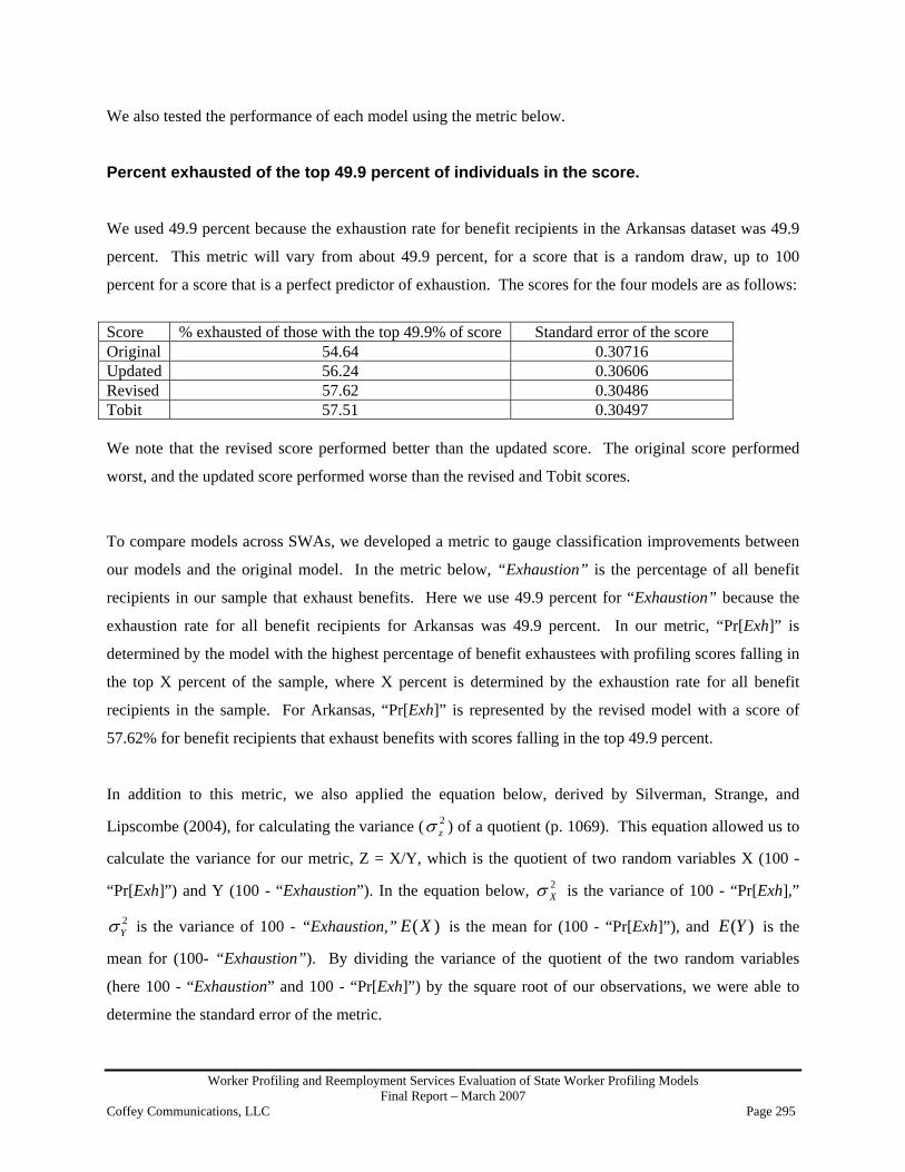
Worker Profiling and Reemployment Services Evaluation of State Worker Profiling Models Final Report – March 2007
Coffey Communications, LLC Page 295
We also tested the performance of each model using the metric below.
Percent exhausted of the top 49.9 percent of individuals in the score.
We used 49.9 percent because the exhaustion rate for benefit recipients in the Arkansas dataset was 49.9
percent. This metric will vary from about 49.9 percent, for a score that is a random draw, up to 100
percent for a score that is a perfect predictor of exhaustion. The scores for the four models are as follows:
Score % exhausted of those with the top 49.9% of score Standard error of the score Original 54.64 0.30716 Updated 56.24 0.30606 Revised 57.62 0.30486 Tobit 57.51 0.30497 We note that the revised score performed better than the updated score. The original score performed
worst, and the updated score performed worse than the revised and Tobit scores.
To compare models across SWAs, we developed a metric to gauge classification improvements between
our models and the original model. In the metric below, “Exhaustion” is the percentage of all benefit
recipients in our sample that exhaust benefits. Here we use 49.9 percent for “Exhaustion” because the
exhaustion rate for all benefit recipients for Arkansas was 49.9 percent. In our metric, “Pr[Exh]” is
determined by the model with the highest percentage of benefit exhaustees with profiling scores falling in
the top X percent of the sample, where X percent is determined by the exhaustion rate for all benefit
recipients in the sample. For Arkansas, “Pr[Exh]” is represented by the revised model with a score of
57.62% for benefit recipients that exhaust benefits with scores falling in the top 49.9 percent.
In addition to this metric, we also applied the equation below, derived by Silverman, Strange, and
Lipscombe (2004), for calculating the variance ( 2zσ ) of a quotient (p. 1069). This equation allowed us to
calculate the variance for our metric, Z = X/Y, which is the quotient of two random variables X (100 -
“Pr[Exh]”) and Y (100 - “Exhaustion”). In the equation below, 2Xσ is the variance of 100 - “Pr[Exh],”
2Yσ is the variance of 100 - “Exhaustion,” )(XE is the mean for (100 - “Pr[Exh]”), and )(YE is the
mean for (100- “Exhaustion”). By dividing the variance of the quotient of the two random variables
(here 100 - “Exhaustion” and 100 - “Pr[Exh]”) by the square root of our observations, we were able to
determine the standard error of the metric.

Worker Profiling and Reemployment Services Evaluation of State Worker Profiling Models Final Report – March 2007
Coffey Communications, LLC Page 296
Metric: 1 – (100 – Pr[Exh]) / (100 – Exhaustion)
Variance of Metric: 4
22
2
22
)()(
)( YEXE
YEYX
zσσ
σ +≈
Standard error of the metric: N
Z2σ
For our metric, “Pr[Exh]” is 57.62 percent and “Exhaustion” is 49.9 percent. We used these to calculate
a score of 0.153495, or roughly 15 percent, with a standard error of 0.00348661. For SWAs with
hypothetically perfect models, this metric will have a value of 1, and for SWAs with models that predict
no better than random, the metric will take a value of 0.
SWA Profiling
score Control for
endogeneity? Exhaustion rate for the
state
Number of individuals
with the highest profiling score
Exhaustion rate for
individuals with high profiling scores
Metric Variance of the Metric
Standard Error of
the metric
Arkansas original score
N 49.9 26,273 54.6 0.095 1.804 0.008
Arkansas revised score N 49.9 26,273 57.6 0.154 1.686 0.008
Analysis of Type I Errors For this analysis, Type I errors occur when individuals who are predicted to exhaust (reject the null
hypothesis), do not exhaust (the null hypothesis is actually true). The analysis is restricted to the top 49.9
percent of individuals who are predicted to exhaust benefits using the revised model.
Variable Mean for
exhausted Mean for non-
exhausted T
statistic P
value N = 15,141 N = 11,133 Potential Duration 20.0119 21.2843 19.0309 0.0000 Ratio of weekly allowance to maximum benefit amount
0.6136 0.6315 5.6053 0.0000
Service Delivery Area 4 0.1137 0.1069 -1.7291 0.0838 Service Delivery Area 5 0.0934 0.0917 -0.4639 0.6427 Service Delivery Area 7 0.0743 0.0817 2.2287 0.0258 Industry 1 0.0141 0.0138 -0.2052 0.8374 Industry 3 0.0828 0.0647 -5.4988 0.0000 Industry 4 0.2316 0.2491 3.2916 0.0010 Industry 7 0.1711 0.1715 0.0879 0.9299 Industry 9 0.2083 0.1983 -1.9834 0.0473

Worker Profiling and Reemployment Services Evaluation of State Worker Profiling Models Final Report – March 2007
Coffey Communications, LLC Page 297
Percentage Change in Industry Employment
12.4168 12.0994 -2.1630 0.0305
Actual Change in Industry Employment 4642.7983 4502.7680 -1.9749 0.0483 Occupation 2 0.0665 0.0585 -2.6466 0.0081 Occupation 5 0.0205 0.0190 -0.8742 0.3820 Occupation 9 0.0821 0.0887 1.8855 0.0594 Low Education Level 0.0230 0.0312 4.0505 0.0001 Insufficient Job Preparation 0.0029 0.0035 0.8522 0.3941 For the above table, 15,141 individuals exhausted benefits and 11,133 did not. The total of these two
types of individuals is 26,274, which is 49.9 percent of the 52,651 individuals in the sample. The Type I
analysis shows that certain variables have more clarifying power than others for explaining the difference
between Type I errors and correct predictions. For example, the variables for occupation 5 and industry 7
are not that important for explaining the difference between exhaustees and non-exhaustees. More
important variables, with low p-values, are potential duration, ratio of weekly allowance to maximum
benefit amount, occupation 2, and industries 3 and 4.

Worker Profiling and Reemployment Services Evaluation of State Worker Profiling Models Final Report – March 2007
Coffey Communications, LLC Page 298
Expanded Analyses of the District of Columbia Profiling
Data

Worker Profiling and Reemployment Services Evaluation of State Worker Profiling Models Final Report – March 2007
Coffey Communications, LLC Page 299
Analysis of District of Columbia Data
Our first step was to replicate the given scores using the data and variable coefficients provided for the
model. From the given data, we identified and replicated variables and categories for unemployment rate,
education level, occupation, industry, base period wages, and job tenure. Our replicated score correlated
with the provided score at .998.
We first developed a decile table for the original score. This table shows for each decile the actual
exhaustion rate, with its standard error and allows us to demonstrate the effectiveness of each model. It
is:
Original score deciles mean se(mean) 1 .4163223 .01585212 .5010438 .01616273 .5333333 .01610994 .5426516 .01597915 .5977249 .015777 6 .5405128 .01596847 .5820106 .01605328 .5964361 .01589259 .643595 .015401610 .6494192 .0155135 Total .5600624 .0050625 We included a binary variable that indicated whether or not benefit recipients were referred to re-
employment services. This binary variable will allow us to test for endogeneity within our data and will
answer the question - does referral to re-employment services have an effect on the exhaustion of
benefits? To test for endogeneity, we first calculated the logit model where only score (and a constant) is
used to predict Pr[exh].
Logit Model with score only Logistic regression Number of obs = 9615 LR chi2(1) = 164.02 Prob > chi2 = 0.0000 Log likelihood = -6513.0601 Pseudo R2 = 0.0124 exhaust Coef. Std. Err. z P>z [95% Conf. Interval] score .002008 .0001587 12.66 0.000 .001697 .0023189 _cons -.81894 .0860793 -9.51 0.000 -.9876522 -.6502277

Worker Profiling and Reemployment Services Evaluation of State Worker Profiling Models Final Report – March 2007
Coffey Communications, LLC Page 300
Adding the variable for referral tests for a uniform referral effect. The test would be a chi-squared test of
difference in the (-2 X log likelihood) statistic for the nested models.
Logit Model with score and referral Logistic regression Number of obs = 9615 LR chi2(2) = 164.92 Prob > chi2 = 0.0000Log likelihood = -6512.6093 Pseudo R2 = 0.0125 exhaust Coef. Std. Err. z P>z [95% Conf. Interval] score .0019831 .0001607 12.34 0.000 .0016681 .0022981 refer -.0667495 .0702656 -0.95 0.342 -.2044675 .0709686 _cons -.7992317 .0884968 -9.03 0.000 -.9726822 -.6257812 The addition of the variable “ref” improved the log likelihood from -6513.0601 to -6512.6093. The
difference in log likelihood was not significant at the .05 level. Our next step was to test for non-uniform
effects. We added an interaction term (referral X score) to test for a non-uniform or unsigned effect.
Logit Model with score, referral and an interaction term Logistic regression Number of obs = 9615 LR chi2(3) = 166.31 Prob > chi2 = 0.0000 Log likelihood = -6511.9149 Pseudo R2 = 0.0126 exhaust Coef. Std. Err. z P>z [95% Conf. Interval] score .0020351 .0001668 12.20 0.000 .0017081 .0023621 refer .2792281 .3011024 0.93 0.354 -.3109217 .869378 scorref -.0007392 .0006251 -1.18 0.237 -.0019644 .0004861 _cons -.8269912 .0916506 -9.02 0.000 -1.006623 -.6473593 The addition of the interaction term changes the log likelihood from -6512.6093 to -6511.9149. The
difference again was not significant. The analysis indicates that there is no need to control for
endogeneity. No offset variable is needed for the further analyses:
Updated Model The updated model for the District of Columbia uses the same variables from the original model to
predict the profiling score, only the coefficients are generated using 2003 data. We include here
diagnostic statistics to show how well the model works, including a classification table that looks at the
top 56 percent of cases (because DC had approximately a 56 percent exhaustion rate for the sample).

Worker Profiling and Reemployment Services Evaluation of State Worker Profiling Models Final Report – March 2007
Coffey Communications, LLC Page 301
Logistic regression Number of obs = 9615 LR chi2(34) = 410.28 Prob > chi2 = 0.0000Log likelihood = -6389.9293 Pseudo R2 = 0.0311 exhaust Coef. Std. Err. z P>z [95% Conf. Interval] tur .0134483 .0020046 6.71 0.000 .0095194 .0173773 edmiss -.1051131 .1687335 -0.62 0.533 -.4358247 .2255985 edlow -.8541375 .1069163 -7.99 0.000 -1.06369 -.6445855 edhsdo -.2015864 .0752988 -2.68 0.007 -.3491694 -.0540033 edcoldo .1127764 .0673605 1.67 0.094 -.0192478 .2448005 edba -.3957758 .0650832 -6.08 0.000 -.5233364 -.2682151 edgraddo -.4033841 .1536708 -2.62 0.009 -.7045734 -.1021949 edmsphd -.5266416 .1107432 -4.76 0.000 -.7436944 -.3095889 occler .1190369 .0743408 1.60 0.109 -.0266683 .2647421 ocserv -.2737408 .0646236 -4.24 0.000 -.4004008 -.1470808 ocaff -.2312374 .3853623 -0.60 0.548 -.9865337 .5240589 ocprocs -.1840963 .3571063 -0.52 0.606 -.8840119 .5158192 octools -.0401533 .3228197 -0.12 0.901 -.6728683 .5925618 ocstruc -.0296399 .1008083 -0.29 0.769 -.2272206 .1679407 ocmiss .2971596 .63288 0.47 0.639 -.9432623 1.537582 ocmisc .3569665 .2220074 1.61 0.108 -.0781601 .792093 indmiss .0360645 .0689763 0.52 0.601 -.0991265 .1712556 oc99 -.3535066 .1117594 -3.16 0.002 -.572551 -.1344622 indcon -.4180692 .1013574 -4.12 0.000 -.616726 -.2194124 indmfg .3583904 .2153035 1.66 0.096 -.0635967 .7803776 indtrn .4711927 .1400267 3.37 0.001 .1967453 .74564 indsal -.2279706 .0713478 -3.20 0.001 -.3678096 -.0881316 indfir .4147907 .1103634 3.76 0.000 .1984824 .631099 indgov -.1533993 .0647095 -2.37 0.018 -.2802277 -.0265709 wg0to7 .3477517 .1087454 3.20 0.001 .1346148 .5608887 wg7to14 .1799942 .083284 2.16 0.031 .0167606 .3432278 wg14to21 .0184585 .0793355 0.23 0.816 -.1370362 .1739531 wg21to28 .0049154 .0823848 0.06 0.952 -.1565559 .1663867 wg35up -.1487703 .0794859 -1.87 0.061 -.3045598 .0070192 jt0to90 -.0380514 .1136005 -0.33 0.738 -.2607042 .1846014 jt91to180 .0185196 .089363 0.21 0.836 -.1566287 .1936679 jt361to720 .1396888 .0661753 2.11 0.035 .0099875 .2693901 jt721to1800 .1504202 .064049 2.35 0.019 .0248865 .2759539 jt1800toup -.103916 .0718191 -1.45 0.148 -.2446788 .0368467 _cons -.4328918 .1465729 -2.95 0.003 -.7201695 -.1456142 -------- True -------- Classified D ~D Total + 3337 1885 5222 - 2048 2345 4393

Worker Profiling and Reemployment Services Evaluation of State Worker Profiling Models Final Report – March 2007
Coffey Communications, LLC Page 302
Total 5385 4230 9615 Sensitivity Pr( + D) 61.97% Specificity Pr( -~D) 55.44% Positive predictive value Pr( D +) 63.90% Negative predictive value Pr(~D -) 53.38% False + rate for true ~D Pr( +~D) 44.56% False - rate for true D Pr( - D) 38.03% False + rate for classified + Pr(~D +) 36.10% False - rate for classified - Pr( D -) 46.62% Correctly classified 59.10% number of observations = 9615 area under ROC curve = 0.6157 The decile table for the updated model is as follows: prupdec mean se(mean) 1 .3711019 .0155839 2 .4657676 .0160745 3 .4973931 .016154 4 .5098855 .0161343 5 .5316719 .0160883 6 .56639 .0159696 7 .6388309 .0155272 8 .635514 .0155173 9 .6690947 .0151866 10 .715625 .0145673 Total .5600624 .0050625 From the original score to the updated model, there was a significant improvement. The decile gradient,
which ranged from .41 to .64 for the original model improved to .37 to .71 for the updated model.
Revised Model The revised model is similar to the updated model, but we incorporated more of the information in the
variable set. We substituted continuous variables for job tenure, education and base period earnings
instead of the categorical versions in the original model. We retained the variable for missing education,
and set those observations to zero in the continuous variable. We also included second order and
interaction terms for the continuous variables to capture nonlinear and discontinuous effects.

Worker Profiling and Reemployment Services Evaluation of State Worker Profiling Models Final Report – March 2007
Coffey Communications, LLC Page 303
We created the second order variables by first centering the variables, by subtracting their mean, and
squaring them. This gave us four variables to measure non-linear effects. We created the interaction
variables by centering and multiplying the four variables, resulting in six additional variables. The means
for the four continuous variables are shown below.
Variable Obs Mean Std. Dev. Min Max Unemployment rate
9615 59.75205 10.69554 21 73
Job tenure 9615 1247.651 1806.014 5 36805 Base period wages
9615 26419.81 23894.42 2031 806357
Education 9461 12.82909 2.678957 1 18 The logit model results for the revised model are as follows. Logistic regression Number of obs = 9615 LR chi2(31) = 449.70 Prob > chi2 = 0.0000Log likelihood = -6370.2206 Pseudo R2 = 0.0341 Exhaust Coef. Std. Err. z P>z [95% Conf. Interval] tur .0142967 .0025944 5.51 0.000 .0092118 .0193816 edmiss -.2664462 .2222356 -1.20 0.231 -.70202 .1691276 edcon -.0249457 .0098782 -2.53 0.012 -.0443067 -.0055847 occler .1263922 .0742144 1.70 0.089 -.0190653 .2718497 ocserv -.2898645 .0646227 -4.49 0.000 -.4165226 -.1632064 ocaff -.2022851 .3834741 -0.53 0.598 -.9538805 .5493102 ocprocs -.2245927 .3573905 -0.63 0.530 -.9250652 .4758797 octools -.0906157 .3225454 -0.28 0.779 -.7227931 .5415617 ocstruc -.0555857 .1012038 -0.55 0.583 -.2539415 .1427701 ocmiss .35076 .6361202 0.55 0.581 -.8960128 1.597533 ocmisc .3759411 .2246645 1.67 0.094 -.0643932 .8162755 indmiss -.0184154 .0680369 -0.27 0.787 -.1517653 .1149345 oc99 -.3676257 .1119282 -3.28 0.001 -.587001 -.1482504 indcon -.4527752 .1023355 -4.42 0.000 -.6533491 -.2522012 indmfg .3852669 .2166544 1.78 0.075 -.0393679 .8099017 indtrn .4424017 .1405375 3.15 0.002 .1669533 .7178501 indsal -.229847 .0712111 -3.23 0.001 -.3694181 -.0902758 indfir .3983932 .1103069 3.61 0.000 .1821955 .6145908 indgov -.1932919 .0645884 -2.99 0.003 -.3198829 -.066701 bpw -7.37e-06 1.56e-06 -4.73 0.000 -.0000104 -4.32e-06 tenure -.0000581 .0000187 -3.10 0.002 -.0000948 -.0000214 xtur2 .000062 .0001562 0.40 0.692 -.0002442 .0003681 xten2 4.56e-09 1.89e-09 2.42 0.016 8.62e-10 8.26e-09 xbpw2 -1.36e-12 9.71e-12 -0.14 0.889 -2.04e-11 1.77e-11

Worker Profiling and Reemployment Services Evaluation of State Worker Profiling Models Final Report – March 2007
Coffey Communications, LLC Page 304
xedu2 -.0163381 .0018357 -8.90 0.000 -.019936 -.0127403 xtute -5.33e-07 1.13e-06 -0.47 0.636 -2.74e-06 1.67e-06 xtubp 5.51e-08 9.75e-08 0.57 0.572 -1.36e-07 2.46e-07 xtued -.0030395 .0008308 -3.66 0.000 -.0046678 -.0014111 xtebp 1.64e-09 5.85e-10 2.81 0.005 4.96e-10 2.79e-09 xteed .0000276 5.66e-06 4.88 0.000 .0000165 .0000387 xbped 6.77e-07 4.74e-07 1.43 0.153 -2.52e-07 1.61e-06 _cons .1419783 .214745 0.66 0.509 -.2789142 .5628709 Classification Table -------- True -------- Classified D ~D Total + 3318 1856 5174 - 2067 2374 4441 Total 5385 4230 9615 Sensitivity Pr( + D) 61.62% Specificity Pr( -~D) 56.12% Positive predictive value Pr( D +) 64.13% Negative predictive value Pr(~D -) 53.46% False + rate for true ~D Pr( +~D) 43.88% False - rate for true D Pr( - D) 38.38% False + rate for classified + Pr(~D +) 35.87% False - rate for classified - Pr( D -) 46.54% Correctly classified 59.20% number of observations = 9615 area under ROC curve = 0.6204 The decile table for the revised model is as follows. prrevdec mean se(mean) 1 .3409563 .0152913 2 .4693028 .016107 3 .491684 .0161268 4 .5109261 .0161336 5 .5602911 .0160113 6 .6024974 .0157947 7 .6070686 .0157549 8 .628512 .0155953 9 .6580042 .0153025 10 .7315297 .014303 Total .5600624 .0050625

Worker Profiling and Reemployment Services Evaluation of State Worker Profiling Models Final Report – March 2007
Coffey Communications, LLC Page 305
This model appears to be an improvement over the updated model. For the updated model, the
exhaustion rate for the deciles ranged from .37 to .71. For the revised model, the deciles range from .34
to .73.
Tobit analysis using the variables of the revised model The following is the procedure we used to generate a Tobit model to predict exhaustion. The Tobit model
is similar to the logit model except that it uses information about non-exhaustees, assuming that non-
exhaustees who are closer to exhaustion are more similar to exhaustees than those who are further from
exhaustion. First, we created a new dependent variable. It is:
100 X (balance of unused UI benefits)/ maximum benefit amount This variable represents the percent of the allowed benefits left to individuals. Exhaustees have a value of 0. Second, we tested for endogeneity using the same procedure as for the logit analyses. Replication is
necessary because of the difference in functional form for the Tobit model. The first model uses only the
score as independent variable.
Tobit regression Number of obs = 9615 LR chi2(1) = 191.27 Prob > chi2 = 0.0000Log likelihood = -7553.2451 Pseudo R2 = 0.0125 tobdep Coef. Std. Err. t P>t [95% Conf. Interval] score -.000758 .000055 -13.78 0.000 -.0008659 -.0006502 _cons .3398938 .0295554 11.50 0.000 .2819589 .3978286 /sigma .633128 .0078806 .6176804 .6485756 The second model uses only score and a binary variable for referred status as independent variables. Tobit regression Number of obs = 9615 LR chi2(2) = 193.26 Prob > chi2 = 0.0000Log likelihood = -7552.2527 Pseudo R2 = 0.0126 tobdep Coef. Std. Err. t P>t [95% Conf. Interval] score -.0007458 .0000557 -13.40 0.000 -.0008549 -.0006366 refer .0345363 .0244905 1.41 0.159 -.0134703 .082543 _cons .3300588 .0303724 10.87 0.000 .2705226 .3895951

Worker Profiling and Reemployment Services Evaluation of State Worker Profiling Models Final Report – March 2007
Coffey Communications, LLC Page 306
/sigma .6330238 .0078792 .617579 .6484686 The addition of the variable “refer” improved the log likelihood from -7553.2451 to -7552.2527. This is
not a significant difference at the 5 percent level. Our next step was to test for non-uniform effects. We
added an interaction term (referral X score) to test for a non-uniform or unsigned effect.
Tobit Model with score, referral and an interaction term Tobit regression Number of obs = 9615 LR chi2(3) = 193.79 Prob > chi2 = 0.0000Log likelihood = -7551.9868 Pseudo R2 = 0.0127 tobdep Coef. Std. Err. t P>t [95% Conf. Interval] score -.0007566 .0000576 -13.13 0.000 -.0008696 -.0006436 refer -.0403752 .1055647 -0.38 0.702 -.2473043 .1665539 scorref .000161 .0002206 0.73 0.466 -.0002714 .0005934 _cons .3358105 .0313733 10.70 0.000 .2743123 .3973088 /sigma .6330194 .0078791 .6175747 .6484641 Here the addition of the interaction term significantly changed the log likelihood from -7552.2527 to -
7551.9868. This difference is again not significant, indicating that there is no significant referral effect.
There is not need to control for endogeneity.
The Tobit model uses the same independent variables as the revised model. The results are as follows. Tobit regression Number of obs = 9615 LR chi2(31) = 428.81 Prob > chi2 = 0.0000 Log likelihood = -7434.4767 Pseudo R2 = 0.0280 tobdep Coef. Std. Err. t P>t [95% Conf. Interval] tur -.0046333 .000895 -5.18 0.000 -.0063877 -.0028789 edmiss .1098075 .0755469 1.45 0.146 -.0382804 .2578954 edcon .0080515 .0033138 2.43 0.015 .0015558 .0145472 occler -.0529211 .0258876 -2.04 0.041 -.1036664 -.0021759 ocserv .1099427 .0221418 4.97 0.000 .0665401 .1533453 ocaff .1094962 .1317675 0.83 0.406 -.1487959 .3677883 ocprocs .1191342 .1216745 0.98 0.328 -.1193735 .357642 octools -.0109415 .1114489 -0.10 0.922 -.2294049 .2075218 ocstruc .0000987 .0345264 0.00 0.998 -.0675804 .0677778 ocmiss -.0869477 .2199987 -0.40 0.693 -.5181917 .3442964

Worker Profiling and Reemployment Services Evaluation of State Worker Profiling Models Final Report – March 2007
Coffey Communications, LLC Page 307
ocmisc -.125542 .0767279 -1.64 0.102 -.2759448 .0248608 indmiss -.0196092 .0236153 -0.83 0.406 -.0659001 .0266818 oc99 .1070987 .0372113 2.88 0.004 .0341566 .1800407 indcon .1381525 .034195 4.04 0.000 .071123 .2051821 indmfg -.1108362 .0749104 -1.48 0.139 -.2576764 .0360039 indtrn -.1850227 .0488638 -3.79 0.000 -.2808061 -.0892392 indsal .0642923 .0243826 2.64 0.008 .0164972 .1120875 indfir -.1519587 .0383993 -3.96 0.000 -.2272295 -.0766879 indgov .0804123 .022207 3.62 0.000 .0368819 .1239428 bpw 2.85e-06 4.75e-07 6.00 0.000 1.92e-06 3.78e-06 tenure .0000239 6.43e-06 3.72 0.000 .0000113 .0000365 xtur2 -.0000197 .0000517 -0.38 0.703 -.0001211 .0000817 xten2 -1.68e-09 6.76e-10 -2.48 0.013 -3.00e-09 -3.53e-10 xbpw2 -1.76e-12 1.46e-12 -1.21 0.227 -4.63e-12 1.10e-12 xedu2 .004419 .0005604 7.89 0.000 .0033205 .0055175 xtute 2.86e-07 3.66e-07 0.78 0.435 -4.31e-07 1.00e-06 xtubp 1.70e-08 3.07e-08 0.55 0.581 -4.32e-08 7.72e-08 xtued .0004772 .0002488 1.92 0.055 -.0000106 .0009649 xtebp -4.67e-10 1.78e-10 -2.62 0.009 -8.16e-10 -1.17e-10 xteed -7.74e-06 1.64e-06 -4.73 0.000 -.0000109 -4.53e-06 xbped -2.74e-07 1.47e-07 -1.87 0.062 -5.62e-07 1.36e-08 _cons -.0325818 .0737347 -0.44 0.659 -.1771173 .1119538 /sigma .624028 .0077549 .6088268 .6392291 The decile table for the Tobit model is as follows. prtobdec mean se(mean) 1 .3482328 .0153681 2 .4745057 .0161164 3 .489605 .0161255 4 .5421436 .01608 5 .539501 .0160786 6 .5712799 .0159726 7 .6205821 .015653 8 .6253902 .0156217 9 .6632017 .0152457 10 .7263267 .0143895 Total .5600624 .0050625 Note that the Tobit model cannot be compared with the logit models by log likelihood comparisons.
However, from the decile tables, the model did not perform substantially better than either the revised
model.
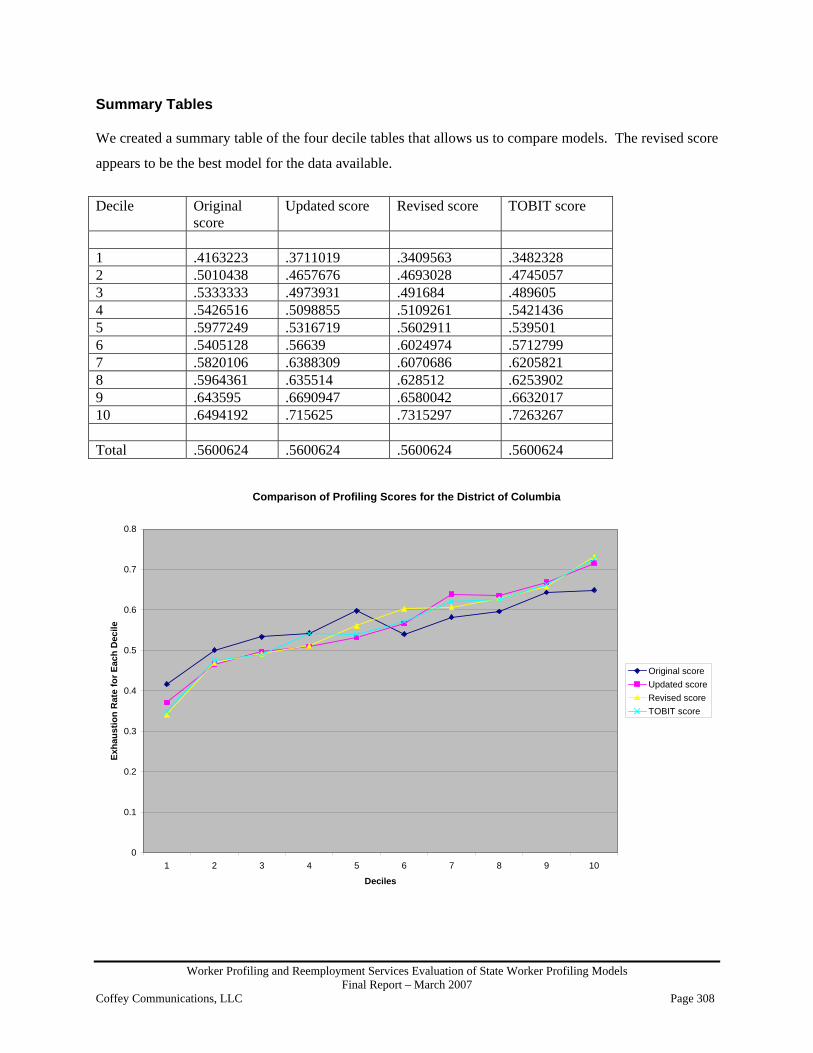
Worker Profiling and Reemployment Services Evaluation of State Worker Profiling Models Final Report – March 2007
Coffey Communications, LLC Page 308
Summary Tables We created a summary table of the four decile tables that allows us to compare models. The revised score
appears to be the best model for the data available.
Decile Original
score Updated score Revised score TOBIT score
1 .4163223 .3711019 .3409563 .3482328 2 .5010438 .4657676 .4693028 .4745057 3 .5333333 .4973931 .491684 .489605 4 .5426516 .5098855 .5109261 .5421436 5 .5977249 .5316719 .5602911 .539501 6 .5405128 .56639 .6024974 .5712799 7 .5820106 .6388309 .6070686 .6205821 8 .5964361 .635514 .628512 .6253902 9 .643595 .6690947 .6580042 .6632017 10 .6494192 .715625 .7315297 .7263267 Total .5600624 .5600624 .5600624 .5600624
Comparison of Profiling Scores for the District of Columbia
0
0.1
0.2
0.3
0.4
0.5
0.6
0.7
0.8
1 2 3 4 5 6 7 8 9 10
Deciles
Exha
ustio
n R
ate
for E
ach
Dec
ile
Original scoreUpdated scoreRevised scoreTOBIT score

Worker Profiling and Reemployment Services Evaluation of State Worker Profiling Models Final Report – March 2007
Coffey Communications, LLC Page 309
Correlations of the four profiling scores indicate that all model scores are positively correlated, as is to be
expected. While the scores are positively correlated, they are not identical, which suggests that there are
differences between the models.
score prup prrev protobn score 1.0000 prup 0.6465 1.0000 prrev 0.5365 0.8392 1.0000 protobn 0.5606 0.8343 0.9776 1.0000 We also tested the performance of each model using the following metric. Percent exhausted of the top 56 percent of individuals in the score. We used 56 percent because that is the exhaustion rate for benefit recipients in the data set provided by
DC. This metric will vary from about 56 percent, for a score that is a random draw, to 100 percent for a
score that is a perfect predictor of exhaustion. The scores for the four models are as follows:
Score % exhausted of those with the top 56% of score Standard error of the score
Original 60.25213 .66639 Updated 63.55366 .65585 Revised 63.76973 .65507 TOBIT 62.93408 .65823 The revised model performs the best, but it is insignificantly better than the updated model. To compare models across SWAs, we developed a metric to gauge classification improvements between
our models and the original model. In the metric below, “Exhaustion” is the percentage of all benefit
recipients in our sample that exhaust benefits. Here we use 56 percent for “Exhaustion” because the
exhaustion rate for all benefit recipients for the District of Columbia was 56 percent. In our metric,
“Pr[Exh]” is determined by the model with the highest percentage of benefit exhaustees with profiling
scores falling in the top X percent of the sample where X percent is determined by the exhaustion rate for
all benefit recipients in the sample. For the District of Columbia, “Pr[Exh]” is represented by the revised
model with a score of 63.77 percent for benefit recipients that exhaust benefits with scores falling in the
top 56 percent.
In addition to this metric, we also applied the equation below, derived by Silverman, Strange, and
Lipscombe (2004), for calculating the variance ( 2zσ ) of a quotient (p. 1069)i. This equation allowed us to
calculate the variance for our metric, Z, which is the quotient of two random variables X and Y where X
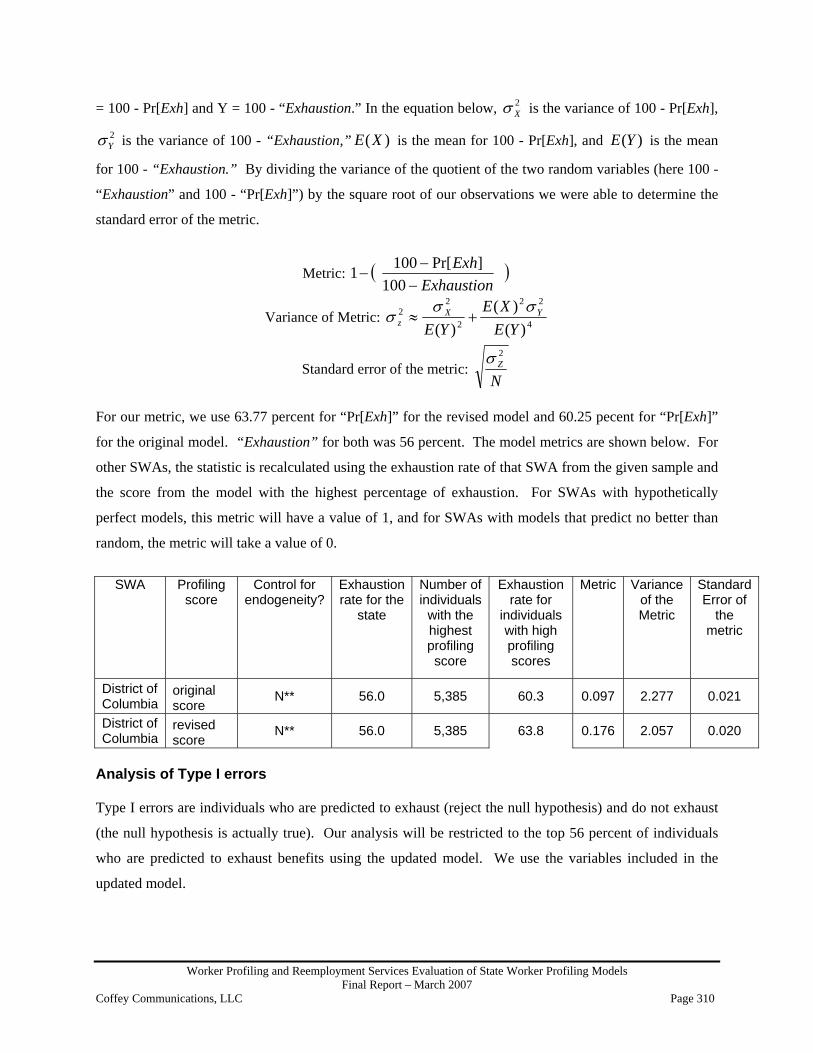
Worker Profiling and Reemployment Services Evaluation of State Worker Profiling Models Final Report – March 2007
Coffey Communications, LLC Page 310
= 100 - Pr[Exh] and Y = 100 - “Exhaustion.” In the equation below, 2Xσ is the variance of 100 - Pr[Exh],
2Yσ is the variance of 100 - “Exhaustion,” )(XE is the mean for 100 - Pr[Exh], and )(YE is the mean
for 100 - “Exhaustion.” By dividing the variance of the quotient of the two random variables (here 100 -
“Exhaustion” and 100 - “Pr[Exh]”) by the square root of our observations we were able to determine the
standard error of the metric.
Metric: ( )Exhaustion
Exh−−
−100
]Pr[1001
Variance of Metric: 4
22
2
22
)()(
)( YEXE
YEYX
zσσ
σ +≈
Standard error of the metric: N
Z2σ
For our metric, we use 63.77 percent for “Pr[Exh]” for the revised model and 60.25 pecent for “Pr[Exh]”
for the original model. “Exhaustion” for both was 56 percent. The model metrics are shown below. For
other SWAs, the statistic is recalculated using the exhaustion rate of that SWA from the given sample and
the score from the model with the highest percentage of exhaustion. For SWAs with hypothetically
perfect models, this metric will have a value of 1, and for SWAs with models that predict no better than
random, the metric will take a value of 0.
SWA Profiling
score Control for
endogeneity? Exhaustion rate for the
state
Number of individuals
with the highest profiling score
Exhaustion rate for
individuals with high profiling scores
Metric Variance of the Metric
Standard Error of
the metric
District of Columbia
original score
N** 56.0 5,385 60.3 0.097 2.277 0.021
District of Columbia
revised score
N** 56.0 5,385 63.8 0.176 2.057 0.020
Analysis of Type I errors Type I errors are individuals who are predicted to exhaust (reject the null hypothesis) and do not exhaust
(the null hypothesis is actually true). Our analysis will be restricted to the top 56 percent of individuals
who are predicted to exhaust benefits using the updated model. We use the variables included in the
updated model.

Worker Profiling and Reemployment Services Evaluation of State Worker Profiling Models Final Report – March 2007
Coffey Communications, LLC Page 311
Variable Mean for exhausted
Mean for non-exhausted
T statistic
P value
N=3,434 N= 1,951 Unemployment rate 63.5300 62.8273 -3.0404 0.0024 Education through 8th grade 0.0116 0.0159 1.3114 0.1898 Education, some high school 0.1040 0.1102 0.7142 0.4751 Education, high school grad 0.5961 0.5664 -2.1284 0.0333 Education, some college 0.1712 0.1589 -1.1672 0.2432 Education, college graduate 0.0612 0.0907 4.0438 0.0001 Education, some graduate school 0.0041 0.0051 0.5552 0.5788 Education, masters or doctorate 0.0058 0.0072 0.6018 0.5473 Education, missing data 0.0154 0.0190 0.9714 0.3314 Occupation, professional and technical
0.2892 0.2932 0.3119 0.7551
Occupation, clerical 0.1514 0.1440 -0.7332 0.4634 Occupation, service 0.1025 0.1005 -0.2383 0.8116 Occupation, agriculture, fish, forest 0.0017 0.0015 -0.1809 0.8564 Occupation, processing 0.0044 0.0031 -0.7315 0.4645 Occupation, machine trades 0.0035 0.0051 0.9019 0.3672 Occupation, benchwork 0.0020 0.0015 -0.4102 0.6817 Occupation, structural 0.0504 0.0436 -1.1248 0.2607 Occupation, miscellaneous 0.0160 0.0118 -1.2480 0.2121 Occupation, missing 0.3789 0.3957 1.2204 0.2224 Industry, construction 0.0160 0.0103 -1.7354 0.0827 Industry, manufacturing 0.0178 0.0149 -0.7977 0.4251 Industry, transportation 0.0475 0.0379 -1.6401 0.1010 Industry, wholesale and retail 0.0964 0.0984 0.2408 0.8097 Industry, finance, insurance and real estate
0.0754 0.0615 -1.9192 0.0550
Industry, government 0.0958 0.1292 3.7969 0.0001 Industry, missing data 0.1570 0.1497 -0.7120 0.4765 Base period wages, $0 to $7,000 0.1174 0.1030 -1.6020 0.1092 Base period wages, $7,000 to $14,000 0.2871 0.2896 0.1921 0.8477 Base period wages, $14,000 to $21,000
0.2504 0.2742 1.9149 0.0556
Base period wages, $21,000 to $28,000
0.1605 0.1486 -1.1477 0.2512
Base period wages, $28,000 to $35,000
0.0874 0.0759 -1.4692 0.1418
Base period wages, $35,000 and above
0.0973 0.1087 1.3321 0.1829
Job tenure, 0 to 90 days 0.0440 0.0528 1.4677 0.1422 Job tenure, 91 to 180 days 0.0981 0.0938 -0.5180 0.6045 Job tenure, 181 to 360 days 0.2545 0.2711 1.3363 0.1815 Job tenure, 361 to 720 days 0.2356 0.2071 -2.4082 0.0161 Job tenure, 721 to 1800 days 0.2598 0.2542 -0.4456 0.6559 Job tenure, more than 1800 days 0.1080 0.1210 1.4417 0.1494

Worker Profiling and Reemployment Services Evaluation of State Worker Profiling Models Final Report – March 2007
Coffey Communications, LLC Page 312
For the table above, note that it includes 3,434 individuals who exhausted benefits and 1,951 who did not.
The total of these two types of individuals is 5,385, which is 56 percent of the 9,615 individuals in the
sample. The Type I analysis shows that certain variables have more explanatory power than others for
explaining the difference between Type I errors and correct predictions. For example, the variables for
unemployment rate and education, college graduate are important for explaining the difference between
exhaustees and non-exhaustees. Less important variables, with low p-values, are occupation, professional
and technical and job tenure, 721 to 1800 days.

Worker Profiling and Reemployment Services Evaluation of State Worker Profiling Models Final Report – March 2007
Coffey Communications, LLC Page 313
Expanded Analyses of Georgia Profiling Data

Worker Profiling and Reemployment Services Evaluation of State Worker Profiling Models Final Report – March 2007
Coffey Communications, LLC Page 314
ANALYSIS OF GEORGIA PROFILING DATA At the time the Georgia survey was completed, the SWA was in the process of programming and
implementing a new linear probability profiling model estimated by ordinary least squares. The new
model is being developed by the W.E. Upjohn Institute. The discussion that follows describes the model
being replaced.
Reported Profiling Model
Currently, Georgia uses a logistical regression model to determine a claimant’s Worker Profiling and
Reemployment Services (WPRS) eligibility. The original model was estimated in 1995 with a sample
size of 10,000. Georgia estimated the existing model in 1998 with a sample size of 77,000 and revised
the model at that time.
Georgia provided their model structure and a dataset for data analysis and possible model revision. From
the given data, we derived variables and categories for education, job tenure, county of residence
unemployment rate, occupation code, and industry code. Further, we successfully replicated the provided
profiling scores. We ranked these profiling scores in ascending order, divided them into deciles, and
produced the decile table shown below. The decile means are calculated by dividing the percentage of
recipients that exhaust benefits for a given decile by 100. For example, in the first decile, our mean is
0.2840939, which indicates that approximately 28 percent of benefit recipients in this decile exhausted
benefits.
Decile Mean Standard Error (Mean) 1 .2840939 .0029731 2 .3311886 .0032492 3 .3382839 .0033743 4 .3436295 .003126 5 .3475689 .0033578 6 .3665276 .0035024 7 .3879867 .0037862 8 .394546 .0039152 9 .405396 .0034609 10 .403749 .0037612 Total .35681 .0010847
For purposes of the analysis, we employed a logistic regression model to ensure that we were able to
properly estimate exhaustibility of benefits using the binary response variables in the original model and

Worker Profiling and Reemployment Services Evaluation of State Worker Profiling Models Final Report – March 2007
Coffey Communications, LLC Page 315
provided in our sample. (Note: we eliminated observations with a value of “0” for maximum benefit
allowance because it is possible that these individuals were erroneously included in the dataset provided.)
Included with the dataset was a binary variable indicating whether or not benefit recipients were referred
to reemployment services. This variable allowed us to test for endogeneity within the data and answer the
question - does referral to reemployment services have an effect on the exhaustion of benefits?
For the analysis, we calculated the logistic regression model where only score (along with a constant) is
used to predict the probability of exhaustion (Pr[exh]).
Logistic Regression Model with Score Only
Logistic regression Number of observations
= 195073
LR chi2(1) = 1133.27 Prob > chi2 = 0.0000 Log likelihood = -126535.26 Pseudo R2 = 0.0045 exh Coefficient Standard
error Z P>z [95% Conf. Interval]
score .022607 .0006742 33.53 0.000 .0212857 .0239283 _cons -1.42629 .0255125 -55.91 0.000 -1.476294 -1.376286 Adding the variable for “referral” tests for a uniform referral effect. The test is a chi-squared test of
difference in the (-2 X log likelihood) statistic for the nested models.
Logistic Regression Model with Score and Referral
Logistic regression Number of observations
= 195073
LR chi2(2) = 5773.78 Prob > chi2 = 0.0000 Log likelihood = -124215 Pseudo R2 = 0.0227 exh Coefficient Standard
error z P>z [95% Conf. Interval]
score .013059 .0006959 18.77 0.000 .011695 .0144229 referred individuals
.7287322 .0106794 68.24 0.000 .707801 .7496633
_cons -1.281733 .0258481 -49.59 0.000 -1.332394 -1.231072

Worker Profiling and Reemployment Services Evaluation of State Worker Profiling Models Final Report – March 2007
Coffey Communications, LLC Page 316
The addition of the variable “referred individuals” improves the log likelihood from -126,535.26 to -
124,215. This represents a significant difference, showing signed or uniform effect. We add an
interaction term (referral X score) to test for a non-uniform or unsigned effect.
Logistic Regression Model with Score, Referral and an Interaction Term
Logistic regression Number of observations = 195073 LR chi2(3) = 5831.32 Prob > chi2 = 0.0000 Log likelihood = -124186.24 Pseudo R2 = 0.0229 exh Coefficient Standard
error z P>z [95% Conf. Interval]
score .0097581 .0008208 11.89 0.000 .0081493 .0113668 referred individuals
.276535 .0606683 4.56 0.000 .1576273 .3954427
referred individuals X score
.0117644 .0015536 7.57 0.000 .0087194 .0148095
_cons -1.162289 .0302252 -38.45 0.000 -1.221529 -1.103048 Again, the addition of the interaction term changes the log likelihood from -124215 to -124186.24. This
represents a significant difference, showing an unsigned or non-uniform effect.
The offset variable is calculated from the referral and interaction variables times their coefficients as:
offset = .276535*referred individuals+ .0117644*cross of referred individuals times score
This value represents the difference between the Pr[exh] for referred and non-referred individuals.
Adding this variable to the logistic regression as a fixed coefficient variable should adjust referred and
exempted individuals to the Pr[exh] that they would have had if they were not referred.
By adjusting the original scores with this control for endogeneity, we can estimate the true exhaustion rate
for the original score. The logistic regression has exhaustion as a dependent variable, score as the
independent variable and the offset, named endogeneity control, to control for endogeneity.
Logistic regression Number of
observations = 195073
Wald chi2(1) = 204.78 Log likelihood = -124186.24
Prob > chi2 = 0.0000

Worker Profiling and Reemployment Services Evaluation of State Worker Profiling Models Final Report – March 2007
Coffey Communications, LLC Page 317
exh Coefficient Standard
error z P>z [95% Conf. Interval]
score .0097581 .0006819 14.31 0.000 .0084216 .0110946 _cons -1.162289 .0257541 -45.13 0.000 -1.212767 -1.111812 endogeneity control
(offset)
By taking the predictions of the model, ordering and dividing them into deciles, and then for each decile
showing the actual exhaustion rate, with its standard error, we obtain the following table that
demonstrates the effectiveness of each model.
Decile Mean Standard Error (Mean) 1 .269121 .0031115 2 .3191817 .0033981 3 .3127325 .0029322 4 .2944923 .0036021 5 .2855699 .0033847 6 .3357326 .0032498 7 .3364993 .0034811 8 .4043413 .0036018 9 .4866126 .0035034 10 .5259009 .0036566 Total .35681 .0010847 By adjusting for endogeneity, our decile gradient improved from a range of a low of 0.28 to a high of 0.40
for the original scores to a low of 0.26 to a high of 0.52.
Updated Profiling Model The updated model has the same form as the original model used to predict score, only the coefficients
are generated using 2003 data. Additionally, the updated model includes the offset to control for
endogeneity. We also include diagnostic statistics to show how well the model works, including a
classification table that looks at the top 36 percent of cases because that is Georgia’s exhaustion rate.
For this model, we are not using a separate model for each geographic (sub-state) area (SSA). Rather, we
are including a binary variable to estimate the variation in exhaustion for each SSA. Unlike in the
original model, this approach does not capture the uniqueness of each region. We are assuming that the
effects for education, tenure, unemployment rate, occupational titles, Standard Industrial Classification
code, and industry change, as measured by their coefficients, will be similar across regions.

Worker Profiling and Reemployment Services Evaluation of State Worker Profiling Models Final Report – March 2007
Coffey Communications, LLC Page 318
The model run showed collinearity between the SSA variables and the industry growth rate, which took
on different values only for each SSA. To correct for this, we used binary variables for only nine of the
eleven SSAs. We dropped the binary variables for SSAs 1 and 2. Similarly, we dropped variables for
edu2 (high school diploma), dot1 (the first type of job title), and sic1 (the first industry classification).
Updated Model Results
Logistic regression Number of observations = 195073 Wald chi2(31) = 3549.15Log likelihood = -122442.98 Prob > chi2 = 0.0000 exh Coefficient Standard
error Z P>z [95% Conf. Interval]
ed1 -.1160946 .0149378 -7.77 0.000 -.1453721 -.086817 ed3 .0771709 .0128641 6.00 0.000 .0519578 .1023841 ed4 .1059333 .0147215 7.20 0.000 .0770797 .1347869 tenure .0324916 .0017111 18.99 0.000 .0291379 .0358453 unemployment rate
.0061226 .0036944 1.66 0.097 -.0011182 .0133634
dot2 .046577 .0132009 3.53 0.000 .0207038 .0724503 dot3 -.1976218 .0187164 -10.56 0.000 -.2343053 -.1609383 dot4 -.1199376 .0599173 -2.00 0.045 -.2373733 -.0025019 dot5 -.2027409 .0447526 -4.53 0.000 -.2904544 -.1150274 dot6 -.1741834 .0244379 -7.13 0.000 -.2220808 -.1262861 dot7 .0625821 .0314 1.99 0.046 .0010392 .1241251 dot8 -.0314562 .0203683 -1.54 0.122 -.0713772 .0084649 dot9 -.0937155 .0177125 -5.29 0.000 -.1284313 -.0589996 sic2 .1716698 .0290238 5.91 0.000 .1147842 .2285555 sic3 .2769711 .032676 8.48 0.000 .2129273 .3410149 sic4 .0746161 .0359445 2.08 0.038 .0041661 .1450661 sic5 .0010642 .0190012 0.06 0.955 -.0361774 .0383057 sic6 .1965589 .0462413 4.25 0.000 .1059277 .2871901 sic7 .3089762 .0214788 14.39 0.000 .2668785 .3510739 sic8 .1053133 .0239066 4.41 0.000 .0584573 .1521694 sic9 .1463108 .0391431 3.74 0.000 .0695917 .2230299 ssa3 .3687098 .0333179 11.07 0.000 .3034079 .4340116 ssa4 -.123113 .0379413 -3.24 0.001 -.1974765 -.0487495 ssa5 .2389732 .0349329 6.84 0.000 .1705059 .3074405 ssa6 -.2439554 .0278371 -8.76 0.000 -.2985151 -.1893956 ssa7 -.2223315 .0306923 -7.24 0.000 -.2824873 -.1621756 ssa8 -.1177148 .0483199 -2.44 0.015 -.2124201 -.0230095 ssa9 -.025174 .0465988 -0.54 0.589 -.116506 .066158 ssa10 -.4014942 .0450889 -8.90 0.000 -.4898669 -.3131216 ssa11 .102602 .035924 2.86 0.004 .0321922 .1730117 industry change
5.656012 3.490768 1.62 0.105 -1.185769 12.49779

Worker Profiling and Reemployment Services Evaluation of State Worker Profiling Models Final Report – March 2007
Coffey Communications, LLC Page 319
_cons -1.101941 .0396315 -27.80 0.000 -1.179618 -1.024265 endogeneity control
(offset)
Classified D ~D Total + 37681 44525 82206 - 31923 80944 112867 Total 69604 125469 195073 Classified + if predicted Pr(D) >= .36 True D defined as exhaust != 0 Sensitivity Pr( + D) 54.14% Specificity Pr( -~D) 64.51% Positive predictive value Pr( D +) 45.84% Negative predictive value Pr(~D -) 71.72% False + rate for true ~D Pr( +~D) 35.49% False - rate for true D Pr( - D) 45.86% False + rate for classified + Pr(~D +) 54.16% False - rate for classified - Pr( D -) 28.28% Correctly classified 60.81% number of observations = 195073 area under ROC curve = 0.6326 The decile table for the updated model is as follows: Decile Mean Standard Error (Mean) 1 .1763198 .0027284 2 .2317355 .0030213 3 .2759027 .0031988 4 .3171106 .0033273 5 .3411982 .0033956 6 .3764332 .0034433 7 .3982042 .003537 8 .4366638 .0035512 9 .49713 .0035795 10 .5180494 .0035781 Total .35681 .0010847 From the change in the log-likelihood, the updated model performed significantly better than the original
model. There is also an improvement in the decile gradient, from a low of 0.27 to a high of 0.53 for the

Worker Profiling and Reemployment Services Evaluation of State Worker Profiling Models Final Report – March 2007
Coffey Communications, LLC Page 320
original model, to a low of 0.18 to a high of 0.52 for the updated model. Also, the updated model shows a
monotonic increase in ability to predict exhaustion.
Revised Model
The revised model is the same as the updated model except that we added 14 more variables to account
for some nonlinear and second-order interaction effects. Two of the variables were second-order versions
of job tenure and unemployment rate. These variables were created by first centering the variables, by
subtracting their mean, and squaring them. A third continuous variable, industry growth rate, was not
included in the second-order effects due to collinearity with the SSA variables. Three interaction terms
were created by centering and multiplying the three second-order combinations (industry growth X job
tenure, industry growth X unemployment rate, and job tenure X unemployment rate). In addition, we
created nine more interaction terms by centering and multiplying job tenure, unemployment rate, and
industrial growth by the three education level binary variables. The means for the variables job tenure,
unemployment rate, and industrial growth are shown below.
Variable Job tenure Unemployment rate Industry growth Mean 4.742332 4.58945 -.0146383 The logistic regression model results for the revised model are as follows. Logistic regression Number of
observations = 195073
Wald chi2(45) = 3707.13 Log likelihood = -122353.66
Prob > chi2 = 0.0000
exh Coefficient Standard
error z P>z [95% Conf. Interval]
ed1 -.1062255 .0156577 -6.78 0.000 -.1369139 -.075537 ed3 .0773488 .0130138 5.94 0.000 .0518422 .1028554 ed4 .1030417 .0157385 6.55 0.000 .0721948 .1338886 tenure .0356726 .002629 13.57 0.000 .0305198 .0408254 unemployment rate
.0295643 .0058729 5.03 0.000 .0180536 .0410751
dot2 .0426767 .0132192 3.23 0.001 .0167676 .0685858 dot3 -.2065151 .018763 -11.01 0.000 -.2432898 -.1697404 dot4 -.1223833 .0599755 -2.04 0.041 -.239933 -.0048336 dot5 -.1961001 .0448341 -4.37 0.000 -.2839733 -.1082269 dot6 -.1746693 .0244739 -7.14 0.000 -.2226372 -.1267014 dot7 .060952 .0314543 1.94 0.053 -.0006973 .1226013

Worker Profiling and Reemployment Services Evaluation of State Worker Profiling Models Final Report – March 2007
Coffey Communications, LLC Page 321
dot8 -.0394995 .020429 -1.93 0.053 -.0795397 .0005406 dot9 -.1013158 .0177572 -5.71 0.000 -.1361192 -.0665123 sic2 .170476 .0290952 5.86 0.000 .1134505 .2275016 sic3 .2762831 .0327473 8.44 0.000 .2120997 .3404665 sic4 .0658167 .0359907 1.83 0.067 -.0047236 .1363571 sic5 -.0031969 .0190607 -0.17 0.867 -.0405553 .0341614 sic6 .1841531 .0462899 3.98 0.000 .0934266 .2748796 sic7 .2999858 .0215617 13.91 0.000 .2577256 .342246 sic8 .0987422 .0239771 4.12 0.000 .0517478 .1457365 sic9 .1427686 .0391897 3.64 0.000 .0659581 .219579 ssa3 .3829197 .0336799 11.37 0.000 .3169082 .4489311 ssa4 -.044004 .0397864 -1.11 0.269 -.1219839 .0339759 ssa5 .1833339 .0359658 5.10 0.000 .1128423 .2538255 ssa6 -.2079831 .0283208 -7.34 0.000 -.2634908 -.1524753 ssa7 -.178459 .0312668 -5.71 0.000 -.2397408 -.1171772 ssa8 -.1984627 .0494136 -4.02 0.000 -.2953115 -.1016138 ssa9 -.0608354 .0470337 -1.29 0.196 -.1530198 .0313491 ssa10 -.4111007 .0452167 -9.09 0.000 -.4997239 -.3224775 ssa11 .1734597 .0376932 4.60 0.000 .0995823 .2473371 industry change
-1.328503 3.712532 -0.36 0.720 -8.604931 5.947925
xt2 .0015943 .0008573 1.86 0.063 -.0000859 .0032745 xu2 -.002237 .000691 -3.24 0.001 -.0035914 -.0008826 xit -.0196541 .3080067 -0.06 0.949 -.6233361 .5840279 xiu -6.78295 .8196579 -8.28 0.000 -8.38945 -5.17645 xtu .0019267 .0009712 1.98 0.047 .0000232 .0038302 xie1 4.17389 2.518685 1.66 0.097 -.7626423 9.110422 xie3 .2940127 2.421071 0.12 0.903 -4.4512 5.039225 xie4 17.17809 2.857317 6.01 0.000 11.57785 22.77832 xte1 .0117554 .0048798 2.41 0.016 .0021911 .0213196 xte3 -.010396 .0043241 -2.40 0.016 -.0188711 -.0019209 xte4 -.0103147 .0048018 -2.15 0.032 -.0197261 -.0009032 xue1 -.0097391 .0077524 -1.26 0.209 -.0249336 .0054553 xue3 -.0081767 .0077511 -1.05 0.291 -.0233686 .0070153 xue4 -.0663594 .0099582 -6.66 0.000 -.0858771 -.0468418 _cons -1.330325 .0491236 -27.08 0.000 -1.426605 -1.234044 endogeneity control
(offset)
Classification Table -------- True -------- Classified D ~D Total + 38391 45387 83778 - 31213 80082 111295 Total 69604 125469 195073

Worker Profiling and Reemployment Services Evaluation of State Worker Profiling Models Final Report – March 2007
Coffey Communications, LLC Page 322
Classified + if predicted Pr(D) >= .36 True D defined as exhaust != 0 Sensitivity Pr( + D) 55.16% Specificity Pr( -~D) 63.83% Positive predictive value
Pr( D +) 45.82%
Negative predictive value
Pr(~D -) 71.95%
False + rate for true ~D
Pr( +~D) 36.17%
False - rate for true D
Pr( - D) 44.84%
False + rate for classified
+ Pr(~D +) 54.18%
False - rate for classified
- Pr( D -) 28.05%
Correctly classified
60.73%
number of observations = 195073 number of covariate patterns = 43883 Pearson chi2(43837) = 43766.92 Prob > chi2 = 0.5927 number of observations = 195073 area under ROC curve = 0.6339 The decile table for the revised model is as follows. Decile Mean Standard Error (Mean) 1 .1748513 .0027196 2 .232582 .003024 3 .2757719 .0032006 4 .3093566 .0033097 5 .3449972 .0034026 6 .3744304 .0034439 7 .4017281 .0034952 8 .4381681 .0035917 9 .4991541 .00358 10 .5182755 .0035776 Total .35681 .0010847 Note that there is a significant improvement from the updated to the revised model in terms of log
likelihood. However, the decile gradient is not much different than the updated model.

Worker Profiling and Reemployment Services Evaluation of State Worker Profiling Models Final Report – March 2007
Coffey Communications, LLC Page 323
Tobit Analysis Using the Variables of the Revised Model Next we analyzed the Georgia data using a Tobit model to predict exhaustion. The Tobit model is similar
to the logistic model except that the Tobit model uses information about non-exhaustees, assuming that
non-exhaustees who are closer to exhaustion are more similar to exhaustees than those claimants who are
further from exhaustion. First, we created a new dependent variable, “/sigma.”
/sigma = 100 X (allowed benefits – benefits paid)/ allowed benefits
This variable represents the percent of the allowed benefits left to individuals. Exhaustees have a value of
0. In the data, all negative values were recoded as 0.
Second, we tested for endogeneity using the same procedure as for the logistic analyses. Replication is
necessary because of the difference in functional form for the Tobit model. The first model uses only the
score as the independent variable.
Tobit regression Number of
observations = 195073
LR chi2(1) = 840.16 Prob > chi2 = 0.0000 Log likelihood = -764544.46 Pseudo R2 = 0.0005 Tobit dependent var.
Coefficient Standard error
t P>t [95% Conf. Interval]
Score -.6311914 .0217849 -28.97 0.000 -.6738892 -.5884935 _cons 59.22275 .8151841 72.65 0.000 57.62501 60.82049 /sigma 64.72412 .1429358 64.44397 65.00427 The second model uses only score and a binary variable for referred status as independent variables. Tobit regression Number of
observations = 195073
LR chi2(2) = 11287.60 Prob > chi2 = 0.0000 Log likelihood = -759320.74 Pseudo R2 = 0.0074 tobit dependent var.
Coefficient Standard error
t P>t [95% Conf. Interval]
score -.1732102 .0215123 -8.05 0.000 -.2153737 -.1310467
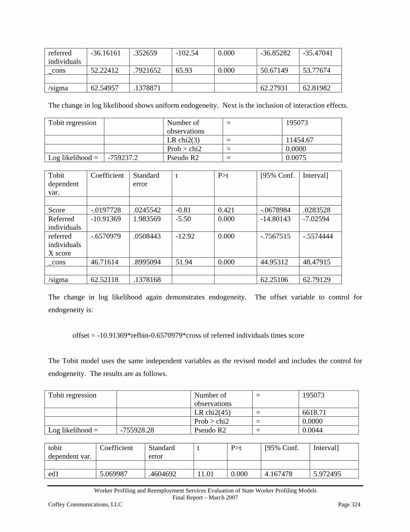
Worker Profiling and Reemployment Services Evaluation of State Worker Profiling Models Final Report – March 2007
Coffey Communications, LLC Page 324
referred individuals
-36.16161 .352659 -102.54 0.000 -36.85282 -35.47041
_cons 52.22412 .7921652 65.93 0.000 50.67149 53.77674 /sigma 62.54957 .1378871 62.27931 62.81982 The change in log likelihood shows uniform endogeneity. Next is the inclusion of interaction effects. Tobit regression Number of
observations = 195073
LR chi2(3) = 11454.67 Prob > chi2 = 0.0000 Log likelihood = -759237.2 Pseudo R2 = 0.0075 Tobit dependent var.
Coefficient Standard error
t P>t [95% Conf. Interval]
Score -.0197728 .0245542 -0.81 0.421 -.0678984 .0283528 Referred individuals
-10.91369 1.983569 -5.50 0.000 -14.80143 -7.02594
referred individuals X score
-.6570979 .0508443 -12.92 0.000 -.7567515 -.5574444
_cons 46.71614 .8995094 51.94 0.000 44.95312 48.47915 /sigma 62.52118 .1378168 62.25106 62.79129 The change in log likelihood again demonstrates endogeneity. The offset variable to control for
endogeneity is:
offset = -10.91369*refbin-0.6570979*cross of referred individuals times score
The Tobit model uses the same independent variables as the revised model and includes the control for
endogeneity. The results are as follows.
Tobit regression Number of
observations = 195073
LR chi2(45) = 6618.71 Prob > chi2 = 0.0000 Log likelihood = -755928.28 Pseudo R2 = 0.0044 tobit dependent var.
Coefficient Standard error
t P>t [95% Conf. Interval]
ed1 5.069987 .4604692 11.01 0.000 4.167478 5.972495

Worker Profiling and Reemployment Services Evaluation of State Worker Profiling Models Final Report – March 2007
Coffey Communications, LLC Page 325
ed3 -3.435752 .3952771 -8.69 0.000 -4.210485 -2.661018 ed4 -8.036164 .4813009 -16.70 0.000 -8.979502 -7.092826 tenure -1.373171 .078728 -17.44 0.000 -1.527476 -1.218866 unemployment rate
-.1843556 .1750566 -1.05 0.292 -.5274624 .1587512
dot2 1.005231 .4092656 2.46 0.014 .2030798 1.807381 dot3 9.884773 .5498551 17.98 0.000 8.807071 10.96248 dot4 6.001274 1.720541 3.49 0.000 2.629054 9.373494 dot5 7.965155 1.266836 6.29 0.000 5.482186 10.44812 dot6 5.950474 .7148331 8.32 0.000 4.549418 7.35153 dot7 -.5867457 .9640386 -0.61 0.543 -2.476238 1.302747 dot8 .0647052 .6091886 0.11 0.915 -1.12929 1.2587 dot9 4.567563 .5292177 8.63 0.000 3.530309 5.604817 sic2 -4.492342 .8568635 -5.24 0.000 -6.171774 -2.81291 sic3 -10.95953 .9934645 -11.03 0.000 -12.9067 -9.012362 sic4 -1.202585 1.069351 -1.12 0.261 -3.298487 .8933164 sic5 1.33033 .5540288 2.40 0.016 .2444472 2.416214 sic6 -5.71412 1.433949 -3.98 0.000 -8.524626 -2.903614 sic7 -10.44492 .6591466 -15.85 0.000 -11.73683 -9.153011 sic8 -2.022165 .7118249 -2.84 0.005 -3.417325 -.6270055 sic9 -3.798288 1.167174 -3.25 0.001 -6.085921 -1.510655 ssa3 -9.767501 .9767781 -10.00 0.000 -11.68196 -7.853039 ssa4 .1852328 1.146887 0.16 0.872 -2.062639 2.433105 ssa5 -5.721148 1.054643 -5.42 0.000 -7.788222 -3.654073 ssa6 8.380592 .8053247 10.41 0.000 6.802175 9.959009 ssa7 5.123843 .8812741 5.81 0.000 3.396567 6.851119 ssa8 8.225395 1.412202 5.82 0.000 5.457513 10.99328 ssa9 4.342947 1.353898 3.21 0.001 1.68934 6.996555 ssa10 15.06619 1.260142 11.96 0.000 12.59634 17.53604 ssa11 -6.950502 1.101365 -6.31 0.000 -9.10915 -4.791854 industry change
133.6846 107.1862 1.25 0.212 -76.3979 343.7671
xt2 -.0601968 .0255331 -2.36 0.018 -.110241 -.0101527 xu2 .0113155 .0209131 0.54 0.588 -.0296737 .0523047 xit 22.9023 9.113746 2.51 0.012 5.039579 40.76503 xiu 233.9308 23.91956 9.78 0.000 187.049 280.8126 xtu .0060012 .0290333 0.21 0.836 -.0509033 .0629057 xie1 -84.06095 72.23 -1.16 0.245 -225.63 57.50813 xie3 37.50738 72.17031 0.52 0.603 -103.9447 178.9595 xie4 -398.8507 87.59991 -4.55 0.000 -570.5444 -227.1569 xte1 -.1988438 .1415403 -1.40 0.160 -.4762594 .0785718 xte3 .2876966 .1313591 2.19 0.029 .0302359 .5451572 xte4 .2370301 .1477318 1.60 0.109 -.0525206 .5265809 xue1 .1671875 .2259057 0.74 0.459 -.2755823 .6099572 xue3 .563227 .2358587 2.39 0.017 .1009495 1.025505 xue4 2.996777 .2981889 10.05 0.000 2.412334 3.58122 _cons 60.20863 1.435741 41.94 0.000 57.39461 63.02265 endogeneity control
(offset)

Worker Profiling and Reemployment Services Evaluation of State Worker Profiling Models Final Report – March 2007
Coffey Communications, LLC Page 326
/sigma 61.20241 .1342908 60.93921 61.46562 The decile table for the Tobit model is as follows. Decile Mean Standard Error (Mean) 1 .1701005 .0026898 2 .2341178 .0030322 3 .2737851 .0031926 4 .3091216 .0033064 5 .3494533 .0034163 6 .3794323 .0034736 7 .3994262 .0035059 8 .4378592 .003554 9 .5052783 .0035792 10 .5096672 .0035801 Total .35681 .0010847 Note that the Tobit model cannot be compared with the logistic regression models by log likelihood
comparisons. However, from the decile tables, the model does not appear to be significantly better than
the revised model.
We created a summary table of the four decile tables that allows us to compare models. The Tobit model
allows only marginal improvement over the revised model. The revised model appears better at
predicting benefit exhaustion than other models.
Decile Original
Score Adjusted Original score
Updated score Revised score Tobit score
1 .2840939 .269121 .1763198 .1748513 .1701005 2 .3311886 .3191817 .2317355 .232582 .2341178 3 .3382839 .3127325 .2759027 .2757719 .2737851 4 .3436295 .2944923 .3171106 .3093566 .3091216 5 .3475689 .2855699 .3411982 .3449972 .3494533 6 .3665276 .3357326 .3764332 .3744304 .3794323 7 .3879867 .3364993 .3982042 .4017281 .3994262 8 .394546 .4043413 .4366638 .4381681 .4378592 9 .405396 .4866126 .49713 .4991541 .5052783 10 .403749 .5259009 .5180494 .5182755 .5096672 Total .35681 .35681 .35681 .35681 .35681

Worker Profiling and Reemployment Services Evaluation of State Worker Profiling Models Final Report – March 2007
Coffey Communications, LLC Page 327
Comparison of the Models for Calculating Profiling Scores
0
0.1
0.2
0.3
0.4
0.5
0.6
1 2 3 4 5 6 7 8 9 10 11
Deciles of score
Exha
ustio
n R
ate
for e
ach
Dec
ile
Original ScoreAdjusted Original scoreUpdated meanRevised meanTobit mean
Correlations of the four profiling scores indicate that the updated, revised, and Tobit scores are highly
correlated. As expected, the original score is positively correlated with the other three scores, though not
at the same magnitude. While the latter three scores are highly correlated, they are not identical, which
suggests that there is a significant difference between the models.
original score updated score revised score tobit score original score 1.0000 updated score 0.3624 1.0000 revised score 0.3827 0.9856 1.0000 tobit score 0.2800 0.9690 0.9754 1.0000 We also tested the performance of each model using the metric below:
Percent exhausted of the top 35.7 percent of individuals in the score.
We used 35.7 percent because the exhaustion rate for benefit recipients in the Georgia dataset was 35.7
percent. This metric will vary from about 35.7 percent, for a score that is a random draw, up to 100
percent for a score that is a perfect predictor of exhaustion. The scores for the four models are as follows:

Worker Profiling and Reemployment Services Evaluation of State Worker Profiling Models Final Report – March 2007
Coffey Communications, LLC Page 328
Score % exhausted of those with the top 35.7% of score Standard error of the score Original 39.83 0.18598 Updated 47.12 0.18926 Revised 47.32 0.18919 Tobit 47.14 0.18925 To compare models across SWAs, we developed a metric to gauge classification improvements between
our models and the original model. In the below metric, “Exhaustion” is the percentage of all benefit
recipients in our sample that exhaust benefits. Here we use 35.7 percent for “Exhaustion” because the
exhaustion rate for all benefit recipients for Georgia was 35.7 percent. In our metric, “Pr[Exh]” is
determined by the model with the highest percentage of benefit exhaustees with profiling scores falling in
the top X percent of the sample, where X percent is determined by the exhaustion rate for all benefit
recipients in the sample. For Georgia, “Pr[Exh]” is represented by the revised model with a score of
47.32 percent for benefit recipients that exhaust benefits with scores falling in the top 35.7 percent.
In addition to this metric, we also applied the equation below, derived by Silverman, Strange, and
Lipscombe (2004), for calculating the variance ( 2zσ ) of a quotient (p. 1069). This equation allowed us to
calculate the variance for our metric, Z = X/Y, which is the quotient of two random variables X (100 -
“Pr[Exh]”) and Y (100 - “Exhaustion”). In the equation below, 2Xσ is the variance of 100 - “Pr[Exh],”
2Yσ is the variance of 100 - “Exhaustion,” )(XE is the mean for (100 - “Pr[Exh]”), and )(YE is the
mean for (100- “Exhaustion”). By dividing the variance of the quotient of the two random variables
(here 100 - “Exhaustion” and 100 - “Pr[Exh]”) by the square root of our observations we were able to
determine the standard error of the metric.
Metric = 1 – (100 - Pr[Exh])/(100 – Exhaustion)
Variance of Metric: 4
22
2
22
)()(
)( YEXE
YEYX
zσσ
σ +≈ where X = ( ]Pr[100 Exh− ), (Y = Exhaustion−100 )
Standard error of the metric: N
Z2σ
For our metric, “Pr[Exh]” is 47.32 percent and “Exhaustion” is 35.7 percent. We used these to calculate
a score of 0.19412879, or roughly 19.4 percent, with a standard error of 0.003648754. For SWAs with
hypothetically perfect models, this metric will have a value of 1, and for SWAs with models that predict
no better than random, the metric will take a value of 0.

Worker Profiling and Reemployment Services Evaluation of State Worker Profiling Models Final Report – March 2007
Coffey Communications, LLC Page 329
SWA Profiling
score Control for
endogeneity? Exhaustion rate for the
state
Number of individuals
with the highest profiling score
Exhaustion rate for
individuals with high profiling scores
Metric Variance of the Metric
Standard Error of
the metric
Georgia original score
Y 35.7 75,994 44.0 0.129 1.017 0.004
Georgia revised score
Y 35.7 75,994 47.3 0.181 0.976 0.004
Analysis of Type I Errors For this analysis, Type I errors occur when individuals who are predicted to exhaust (reject the null
hypothesis) do not exhaust (the null hypothesis is actually true). The analysis is restricted to the top 35.7
percent of individuals who are predicted to exhaust benefits using the revised model.
Variable Mean for exhausted Mean for non-exhausted T statistic P value N=32,953 N=36,692 Education < HS diploma 0.0835 0.0899 -3.0051 0.0027 Education = HS diploma 0.3152 0.3418 -7.4620 0.0000 Education=some college 0.2828 0.2910 -2.4072 0.0161 Education=college grad+ 0.3185 0.2772 11.8840 0.0000 Job tenure 6.0272 5.9909 1.7969 0.0724 Local unemployment rate 4.3973 4.4445 -3.7872 0.0002 Occupation type 1 0.4521 0.4253 7.1061 0.0000 Occupation type 2 0.3136 0.3394 -7.2346 0.0000 Occupation type 3 0.0476 0.0571 -5.6671 0.0000 Occupation type 4 0.0042 0.0036 1.3132 0.1891 Occupation type 5 0.0064 0.0076 -1.7814 0.0748 Occupation type 6 0.0279 0.0252 2.1327 0.0330 Occupation type 7 0.0325 0.0345 -1.4783 0.1393 Occupation type 8 0.0540 0.0469 4.2548 0.0000 Occupation type 9 0.0618 0.0604 0.7489 0.4539 Industry class 0 0.7202 0.7096 3.1101 0.0019 Industry class 1 0.0137 0.0132 0.4840 0.6284 Industry class 2 0.0267 0.0294 -2.1991 0.0279 Industry class 3 0.0283 0.0273 0.8050 0.4208 Industry class 4 0.0152 0.0168 -1.5945 0.1108 Industry class 5 0.0425 0.0507 -5.1513 0.0000 Industry class 6 0.0161 0.0171 -1.0117 0.3117 Industry class 7 0.0782 0.0770 0.5624 0.5738 Industry class 8 0.0438 0.0435 0.1809 0.8565 Industry class 9 0.0153 0.0153 -0.0347 0.9723 Area 1 0.0350 0.0391 -2.8612 0.0042 Area 2 0.0588 0.0596 -0.4558 0.6485

Worker Profiling and Reemployment Services Evaluation of State Worker Profiling Models Final Report – March 2007
Coffey Communications, LLC Page 330
Area 3 0.7188 0.7155 0.9458 0.3442 Area 4 0.0248 0.0228 1.7366 0.0825 Area 5 0.0313 0.0317 -0.2995 0.7645 Area 6 0.0316 0.0334 -1.2929 0.1960 Area 7 0.0196 0.0171 2.4352 0.0149 Area 8 0.0163 0.0173 -1.0847 0.2781 Area 9 0.0311 0.0308 0.2477 0.8043 Area 10 0.0050 0.0049 0.0829 0.9339 Area 11 0.0277 0.0277 0.0089 0.9929 Industry growth rate -0.0161 -0.0162 0.3443 0.7306 For the above table, 32,953 individuals exhausted benefits and 36,692 did not. The total of these two
types of individuals is 69,645, which is 35.7 percent of the 195,073 individuals in the sample. The Type I
analysis shows that certain variables have more explanatory power than others for explaining the
difference between Type I errors and correct predictions. For example, the area variables are not that
important for explaining the difference between exhaustees and non-exhaustees. More important
variables, with low p-values, are education = High School diploma, education = college grad+, local
unemployment rate and occupation types 1, 2, and 3.

Worker Profiling and Reemployment Services Evaluation of State Worker Profiling Models Final Report – March 2007
Coffey Communications, LLC Page 331
Expanded Analyses of Hawaii Profiling Data

Worker Profiling and Reemployment Services Evaluation of State Worker Profiling Models Final Report – March 2007
Coffey Communications, LLC Page 332
Analysis of Hawaii Data
For our analysis, we employed a logit model to predict exhaustibility similar to the logit model used by
Hawaii to calculate the original profiling scores. We did this to ensure that we were able to properly
estimate exhaustibility of benefits using the binary response variables used in the original model and
provided in our sample.
Our first step was to replicate the given scores using the data and variable coefficients provided for the
model. From the given data, we identified and replicated variables and categories for county total
unemployment rate, education level, industry code, occupation code, job tenure, and weekly benefit
amount. We noticed that there were four cases that were outliers, one with no profiling score and three
with scores that were at least ten times that of the other scores. The correlation of our replicated score
with the original profiling score was only .42. The elimination of the four outlier cases reduced the
sample from 8976 to 8972, and we were able to develop a score that correlated with the original score at a
level of .86. Our analysis proceeded with the revised sample.
Another problem with the data is that there was little variation in occupation. Of the 8,972 cases, 8,969
were occupation 1 - professional, technical, managerial. One was occupation 4 - agricultural, fishery,
forestry, and two were occupation 8 - structural work. We suspect that the data are incomplete for the
occupation variable, but the high correlation shows that this omission is not serious. In our analyses
below, we will not include occupation variables.
We first developed a decile table for the original score. This table shows for each decile the actual
exhaustion rate, with its standard error and allows us to demonstrate the effectiveness of each model. It
is:
Original score deciles mean se(mean) 1 .320356 .01557112 .359375 .01603853 .3489409 .01592334 .3534002 .01596975 .4087432 .01626076 .3886364 .016441 7 .4197121 .01643218 .4480088 .01654889 .4366516 .016690710 .4548495 .0166356 Total .3938921 .0051587

Worker Profiling and Reemployment Services Evaluation of State Worker Profiling Models Final Report – March 2007
Coffey Communications, LLC Page 333
Also included was a binary variable that indicated whether or not benefit recipients were referred to re-
employment services. This binary variable will allow us to test for endogeneity within our data and will
answer the question - does referral to re-employment services have an effect on the exhaustion of
benefits? To test for endogeneity, we first calculated the logit model where only score (and a constant) is
used to predict Pr[exh].
Logit Model with score only Logistic regression Number of obs = 8972 LR chi2(1) = 69.82 Prob > chi2 = 0.0000 Log likelihood = -5980.4347 Pseudo R2 = 0.0058 exhaust Coef. Std. Err. z P>z [95% Conf. Interval] scorereal 2.241093 .269989 8.30 0.000 1.711924 2.770261 _cons -1.456022 .1258169 -11.57 0.000 -1.702618 -1.209425 Adding the variable for referral tests for a uniform referral effect. The test would be a chi-squared test of
difference in the (-2 X log likelihood) statistic for the nested models.
Logit Model with score and referral Logistic regression Number of obs = 8972 LR chi2(2) = 73.72 Prob > chi2 = 0.0000 Log likelihood = -5978.484
Pseudo R2 = 0.0061
exhaust Coef. Std. Err. z P>z [95% Conf. Interval] scorereal 2.607491 .3284657 7.94 0.000 1.96371 3.251272 refer -.1039734 .0526927 -1.97 0.048 -.2072491 -.0006977 _cons -1.572106 .1392873 -11.29 0.000 -1.845105 -1.299108 The addition of the variable “refer” improved the log likelihood from -5980.4347 to -5978.484. The
difference in log likelihood was 1.95, which is significant at the .05 level. Our next step was to test for
non-uniform effects. We added an interaction term (referral X score) to test for a non-uniform or
unsigned effect.

Worker Profiling and Reemployment Services Evaluation of State Worker Profiling Models Final Report – March 2007
Coffey Communications, LLC Page 334
Logit Model with score, referral and an interaction term Logistic regression Number of obs = 8972 LR chi2(3) = 73.87 Prob > chi2 = 0.0000 Log likelihood = -5978.4087 Pseudo R2 = 0.0061 exhaust Coef. Std. Err. z P>z [95% Conf. Interval] scorereal 2.474107 .4751427 5.21 0.000 1.542844 3.405369 refer -.2206746 .3053479 -0.72 0.470 -.8191454 .3777963 xrefscore .2553012 .6578512 0.39 0.698 -1.034064 1.544666 _cons -1.516941 .1988522 -7.63 0.000 -1.906685 -1.127198 The addition of the interaction term changes the log likelihood from -5978.484 to -5978.4087. The
difference was not significant. The analysis indicates that there is only a need to control for uniform
endogeneity. The offset variable is as follows:
-.1039734*refer After correcting for endogeneity, we obtain the following decile table. prorigdec mean se(mean) 1 .3273942 .0156682 2 .3143813 .0155101 3 .3756968 .0161794 4 .3756968 .0161794 5 .4046823 .0163975 6 .3886414 .0162752 7 .406015 .0161034 8 .4229432 .0168266 9 .4570792 .0166422 10 .4671126 .0166677 Total .3938921 .0051587 Updated Model The updated model for Hawaii uses the same variables as used in the original model to predict the
profiling score, only the coefficients are generated using 2003 data. We also included diagnostic statistics
to show how well the model works, including a classification table that looks at the top 39.3 percent of
cases (because Hawaii has approximately a 39.3 percent exhaustion rate for the 8,972 cases in our
analysis). As noted above, we did not use the occupation variable because of the lack of variation.

Worker Profiling and Reemployment Services Evaluation of State Worker Profiling Models Final Report – March 2007
Coffey Communications, LLC Page 335
Logistic regression Number of obs = 8972 Wald chi2(8) = 102.90Log likelihood = -5973.5191 Prob > chi2 = 0.0000Logistic regression Number of obs = 8972 exhaust Coef. Std. Err. z P>z [95% Conf. Interval] tur -.0391454 .0146026 -2.68 0.007 -.0677659 -.0105249 edu1 -.0011308 .0817388 -0.01 0.989 -.1613359 .1590743 edu3 .0196977 .0574813 0.34 0.732 -.0929636 .132359 edu4 -.1030133 .0678498 -1.52 0.129 -.2359965 .0299699 edu5 -.5466895 .1615675 -3.38 0.001 -.863356 -.230023 indchg .0081247 .0041752 1.95 0.052 -.0000585 .0163078 tenure .0132191 .0037979 3.48 0.001 .0057754 .0206629 wba .0012269 .0001768 6.94 0.000 .0008804 .0015734 _cons -.5474571 .0814076 -6.72 0.000 -.7070131 -.3879011 offset (offset) -------- True -------- Classified D ~D Total + 1793 2344 4137 - 1741 3094 4835 Total 3534 5438 8972 Classified + if predicted Pr(D) >= .393True D defined as exhaust != 0 Sensitivity Pr( + D) 50.74% Specificity Pr( -~D) 56.90% Positive predictive value Pr( D +) 43.34% Negative predictive value Pr(~D -) 63.99% False + rate for true ~D Pr( +~D) 43.10% False - rate for true D Pr( - D) 49.26% False + rate for classified + Pr(~D +) 56.66% False - rate for classified - Pr( D -) 36.01% Correctly classified 54.47% number of observations = 8972 area under ROC curve = 0.5569 The decile table for the updated model is as follows:

Worker Profiling and Reemployment Services Evaluation of State Worker Profiling Models Final Report – March 2007
Coffey Communications, LLC Page 336
prupdec mean se(mean) 1 .2817372 .0150199 2 .3322185 .0157353 3 .3730512 .0161475 4 .4129464 .0164579 5 .386845 .0162705 6 .4153675 .0164536 7 .4292085 .0165356 8 .3908686 .016292 9 .4424779 .0165285 10 .4746907 .0167574 Total .3938921 .0051587 From the original score to the updated model, there was a significant improvement. The decile gradient,
which ranged from .327 to .467 for the original model (corrected for endogeneity) improved to .282 to
.474 for the updated model.
Revised Model The revised model is similar to the updated model, but we incorporated more of the information in the
variable set. We included second order terms to capture nonlinear and discontinuous effects, which
differs from the original model. The original model used a series of categories to account for these
effects. The revised model consists of the following variables.
• Categorical variables for industry and local office
• Continuous variables for job tenure, weekly benefit amount (wba), education, total county
unemployment rate, and industry employment percentage change (indchg)
• Second order variables for tenure, wba, educ, and indchg
• And interaction variables for tenure X wba, tenure X educ, tenure X indchg, wba X educ, wba X
indchg, and educ X indchg
The revised model basically replaces the categorical variable for education with a continuous variable,
adds variables for office and industry, and includes second order and interaction effects.
We created the second order variable by first centering the variables, by subtracting their mean, and
squaring them. We created the interaction variables by centering and multiplying the three second order
combinations. The means for the three continuous variables are shown below.
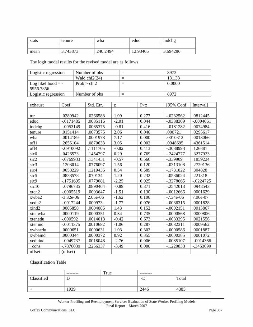
Worker Profiling and Reemployment Services Evaluation of State Worker Profiling Models Final Report – March 2007
Coffey Communications, LLC Page 337
stats tenure wba educ indchg mean 3.743873 240.2494 12.93405 3.694286 The logit model results for the revised model are as follows. Logistic regression Number of obs = 8972 Wald chi2(24) = 131.33 Log likelihood = -5956.7856
Prob > chi2 = 0.0000
Logistic regression Number of obs = 8972 exhaust Coef. Std. Err. z P>z [95% Conf. Interval] tur .0289942 .0266588 1.09 0.277 -.0232562 .0812445 educ -.0171485 .0085116 -2.01 0.044 -.0338309 -.0004661 indchg -.0053149 .0065375 -0.81 0.416 -.0181282 .0074984 tenure .0151414 .0073575 2.06 0.040 .000721 .0295617 wba .0014189 .0001978 7.17 0.000 .0010312 .0018066 off1 .2655104 .0870633 3.05 0.002 .0948695 .4361514 off4 -.0910092 .1111705 -0.82 0.413 -.3088993 .126881 sic0 .0426573 .1454797 0.29 0.769 -.2424777 .3277923 sic2 -.0769933 .1341431 -0.57 0.566 -.339909 .1859224 sic3 .1208014 .0776097 1.56 0.120 -.0313108 .2729136 sic4 .0658229 .1219436 0.54 0.589 -.1731822 .304828 sic5 .0838578 .070134 1.20 0.232 -.0536024 .221318 sic9 -.1751695 .0779081 -2.25 0.025 -.3278665 -.0224725 sic10 -.0796735 .0890464 -0.89 0.371 -.2542013 .0948543 xten2 -.0005519 .0003647 -1.51 0.130 -.0012666 .0001629 xwba2 -3.32e-06 2.05e-06 -1.62 0.106 -7.34e-06 7.06e-07 xedu2 -.0017244 .000973 -1.77 0.076 -.0036315 .0001828 xind2 .0005858 .0004086 1.43 0.152 -.0002151 .0013867 xtenwba .0000119 .0000351 0.34 0.735 -.0000568 .0000806 xtenedu -.000592 .0014018 -0.42 0.673 -.0033395 .0021556 xtenind -.0011375 .0010682 -1.06 0.287 -.0032311 .0009562 xwbaedu .0000651 .0000631 1.03 0.302 -.0000586 .0001887 xwbaind .0000344 .0000372 0.92 0.355 -.0000385 .0001072 xeduind -.0049737 .0018046 -2.76 0.006 -.0085107 -.0014366 _cons -.7876039 .2256337 -3.49 0.000 -1.229838 -.3453699 offset (offset) Classification Table -------- True -------- Classified D ~D Total + 1939 2446 4385

Worker Profiling and Reemployment Services Evaluation of State Worker Profiling Models Final Report – March 2007
Coffey Communications, LLC Page 338
- 1595 2992 4587 Total 3534 5438 8972 Classified + if predicted Pr(D) >= .393True D defined as exhaust != 0 Sensitivity Pr( + D) 54.87% Specificity Pr( -~D) 55.02% Positive predictive value
Pr( D +) 44.22%
Negative predictive value
Pr(~D -) 65.23%
False + rate for true ~D
Pr( +~D) 44.98%
False - rate for true D
Pr( - D) 45.13%
False + rate for classified
+ Pr(~D +) 55.78%
False - rate for classified
- Pr( D -) 34.77%
Correctly classified
54.96%
number of observations = 8972 area under ROC curve = 0.5682 The decile table for the revised model is as follows. prrevdec mean se(mean) 1 .3084633 .015421 2 .3188406 .0155689 3 .3377926 .0158004 4 .3846154 .016253 5 .3734671 .0161601 6 .422049 .0164904 7 .4225195 .0165021 8 .4180602 .016478 9 .4537347 .0166322 10 .4994426 .0167038 Total .3938921 .0051587 This model appears to be similar to the updated model.
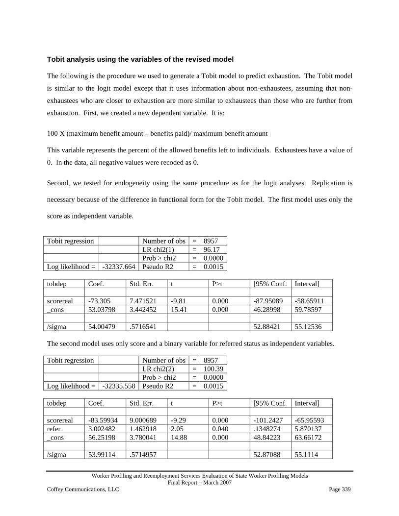
Worker Profiling and Reemployment Services Evaluation of State Worker Profiling Models Final Report – March 2007
Coffey Communications, LLC Page 339
Tobit analysis using the variables of the revised model The following is the procedure we used to generate a Tobit model to predict exhaustion. The Tobit model
is similar to the logit model except that it uses information about non-exhaustees, assuming that non-
exhaustees who are closer to exhaustion are more similar to exhaustees than those who are further from
exhaustion. First, we created a new dependent variable. It is:
100 X (maximum benefit amount – benefits paid)/ maximum benefit amount This variable represents the percent of the allowed benefits left to individuals. Exhaustees have a value of
0. In the data, all negative values were recoded as 0.
Second, we tested for endogeneity using the same procedure as for the logit analyses. Replication is
necessary because of the difference in functional form for the Tobit model. The first model uses only the
score as independent variable.
Tobit regression Number of obs = 8957 LR chi2(1) = 96.17 Prob > chi2 = 0.0000Log likelihood = -32337.664 Pseudo R2 = 0.0015 tobdep Coef. Std. Err. t P>t [95% Conf. Interval] scorereal -73.305 7.471521 -9.81 0.000 -87.95089 -58.65911 _cons 53.03798 3.442452 15.41 0.000 46.28998 59.78597 /sigma 54.00479 .5716541 52.88421 55.12536 The second model uses only score and a binary variable for referred status as independent variables. Tobit regression Number of obs = 8957 LR chi2(2) = 100.39 Prob > chi2 = 0.0000Log likelihood = -32335.558 Pseudo R2 = 0.0015 tobdep Coef. Std. Err. t P>t [95% Conf. Interval] scorereal -83.59934 9.000689 -9.29 0.000 -101.2427 -65.95593 refer 3.002482 1.462918 2.05 0.040 .1348274 5.870137 _cons 56.25198 3.780041 14.88 0.000 48.84223 63.66172 /sigma 53.99114 .5714957 52.87088 55.1114

Worker Profiling and Reemployment Services Evaluation of State Worker Profiling Models Final Report – March 2007
Coffey Communications, LLC Page 340
The addition of the variable “refer” improved the log likelihood from -32,337.664 to -32,335.558. This is
a significant difference. Our next step was to test for non-uniform effects. We added an interaction term
(referral X score) to test for a non-uniform or unsigned effect.
Tobit Model with score, referral and an interaction term Tobit regression Number of obs = 8957 LR chi2(3) = 100.82 Prob > chi2 = 0.0000Log likelihood = -32335.339 Pseudo R2 = 0.0016 tobdep Coef. Std. Err. t P>t [95% Conf. Interval] scorereal -77.37716 13.01251 -5.95 0.000 -102.8847 -51.86966 refer 8.399741 8.285013 1.01 0.311 -7.840782 24.64026 xrefscore -11.91289 17.99937 -0.66 0.508 -47.19578 23.37001 _cons 53.70331 5.396295 9.95 0.000 43.12533 64.28128 /sigma 53.98965 .571478 52.86943 55.10988 Here the addition of the interaction term significantly changed the log likelihood from -32,335.558 to -
32,335.339. This difference is not significant, indicating only a uniform endogeneity. The offset variable
to control for endogeneity is:
3.002482*refer The Tobit model uses the same independent variables as the revised model, and includes the Tobit control
for endogeneity. The results are as follows.
Tobit regression Number of obs = 8957 LR chi2(24) = 192.19 Prob > chi2 = 0.0000 Log likelihood = -32301.934 Pseudo R2 = 0.0030 tobdep Coef. Std. Err. t P>t [95% Conf. Interval] tur -.3451683 .7293353 -0.47 0.636 -1.774833 1.084496 educ .2863111 .2033531 1.41 0.159 -.1123075 .6849298 indchg .1332884 .181889 0.73 0.464 -.2232558 .4898326 tenure -.4894389 .2069076 -2.37 0.018 -.8950253 -.0838526 wba -.0476838 .0054322 -8.78 0.000 -.0583322 -.0370355 off1 -7.545566 2.377297 -3.17 0.002 -12.20561 -2.885519 off4 1.632075 3.019966 0.54 0.589 -4.287751 7.551901 sic0 -3.712503 4.026695 -0.92 0.357 -11.60575 4.180743 sic2 3.638701 3.677433 0.99 0.322 -3.569911 10.84731

Worker Profiling and Reemployment Services Evaluation of State Worker Profiling Models Final Report – March 2007
Coffey Communications, LLC Page 341
sic3 -6.391724 2.205565 -2.90 0.004 -10.71514 -2.068311 sic4 .8271065 3.439165 0.24 0.810 -5.914446 7.568659 sic5 -1.940512 1.959434 -0.99 0.322 -5.781453 1.900428 sic9 7.05395 2.100153 3.36 0.001 2.937167 11.17073 sic10 2.953944 2.450827 1.21 0.228 -1.85024 7.758127 xten2 .0166888 .010239 1.63 0.103 -.003382 .0367595 xwba2 .0001105 .0000554 2.00 0.046 1.95e-06 .0002191 xedu2 .0118038 .0071749 1.65 0.100 -.0022606 .0258682 xind2 -.0148024 .0113823 -1.30 0.193 -.0371144 .0075096 xtenwba -.000074 .0009701 -0.08 0.939 -.0019755 .0018276 xtenedu .0456322 .039288 1.16 0.245 -.0313813 .1226458 xtenind .0217588 .0303875 0.72 0.474 -.0378077 .0813253 xwbaedu -.0006531 .001685 -0.39 0.698 -.003956 .0026498 xwbaind -.0012345 .0010308 -1.20 0.231 -.0032552 .0007862 xeduind .1096415 .0480574 2.28 0.023 .0154378 .2038451 _cons 31.7311 5.910246 5.37 0.000 20.14566 43.31654 tobend (offset) The decile table for the Tobit model is as follows. prtobdec mean se(mean) 1 .3162584 .0155264 2 .3054627 .0153877 3 .361204 .0160474 4 .4024526 .0163829 5 .3723523 .0161503 6 .4053452 .0163926 7 .4158305 .0164655 8 .4091416 .0164257 9 .4537347 .0166322 10 .4972129 .0167036 Total .3938921 .0051587 Note that the Tobit model cannot be compared with the logit models by log likelihood comparisons.
However, from the decile tables, the model did not perform substantially better than either the updated or
revised models.
We created a summary table of the four decile tables that allows us to compare models. While there was
considerable improvement between the updated and revised models, there was no improvement with the
Tobit model. The updated model appears to be the best model for the data available.

Worker Profiling and Reemployment Services Evaluation of State Worker Profiling Models Final Report – March 2007
Coffey Communications, LLC Page 342
Decile Original score
Original score adapted for endogeneity
Updated mean Revised mean Tobit mean
1 .320356 .3273942 .2817372 .3084633 .3162584 2 .359375 .3143813 .3322185 .3188406 .3054627 3 .3489409 .3756968 .3730512 .3377926 .361204 4 .3534002 .3756968 .4129464 .3846154 .4024526 5 .4087432 .4046823 .386845 .3734671 .3723523 6 .3886364 .3886414 .4153675 .422049 .4053452 7 .4197121 .406015 .4292085 .4225195 .4158305 8 .4480088 .4229432 .3908686 .4180602 .4091416 9 .4366516 .4570792 .4424779 .4537347 .4537347 10 .4548495 .4671126 .4746907 .4994426 .4972129 Total .3938921 .3938921 .3938921 .3938921 .3938921
Comparison of Profiling Scores for Hawaii
0
0.1
0.2
0.3
0.4
0.5
0.6
1 2 3 4 5 6 7 8 9 10
Deciles
Prop
ortio
n W
ho E
xhau
sted
Ben
efits
original scoreadapted original scoreupdated scorerevised scoreTOBIT score
Correlations of the five profiling scores indicate that all model scores are positively correlated, as is to be
expected. While the scores are positively correlated, they are not identical, which suggests that there are
differences between the models. Note, the strongest correlation is between the revised and Tobit models
with a correlation of 0.96.

Worker Profiling and Reemployment Services Evaluation of State Worker Profiling Models Final Report – March 2007
Coffey Communications, LLC Page 343
scorereal prorig prup prrev protobnscorereal 1.0000 prorig 0.9742 1.0000 prup 0.7231 0.6816 1.0000 prrev 0.6830 0.6780 0.7227 1.0000 protobn 0.6813 0.6715 0.7274 0.9616 1.0000 We also tested the performance of each model using the following metric. Percent exhausted of the top 39.3 percent of individuals in the score. We used 39.3 percent because the exhaustion rate for benefit recipients in the data set provided by Hawaii
was 39.3 percent. This metric will vary from about 39.3 percent, for a score that is a random draw, to 100
percent for a score that is a perfect predictor of exhaustion. The scores for the four models are as follows:
Score % exhausted of those with the top 39.3% of score Standard error of the score
Original 43.87408 .83581 Adapted 43.87408 .83581 Updated 43.2785 .83451 Revised 44.81293 .83737 TOBIT 44.36281 .83524 To compare models across SWAs, we developed a metric to gauge classification improvements between
our models and the original model. In the below metric, “Exhaustion” is the percentage of all benefit
recipients in our sample that exhaust benefits. Here we use 39.3 percent for “Exhaustion” because the
exhaustion rate for all benefit recipients for Hawaii was 39.3 percent. In our metric, “Pr[Exh]” is
determined by the model with the highest percentage of benefit exhaustees with profiling scores falling in
the top X percent of the sample where X percent is determined by the exhaustion rate for all benefit
recipients in the sample. For Hawaii, “Pr[Exh]” is represented by the revised model with a score of 44.38
percent for benefit recipients that exhaust benefits with scores falling in the top 39.3 percent.
In addition to this metric we also applied the equation below, derived by Silverman, Strange, and
Lipscombe (2004), for calculating the variance ( 2zσ ) of a quotient (p. 1069)ii. This equation allowed us to
calculate the variance for our metric, Z, which is the quotient of two random variables X and Y where X
= 100 - Pr[Exh] and Y = 100 - “Exhaustion.” In the equation below, 2Xσ is the variance of 100 - Pr[Exh],
2Yσ is the variance of 100 - “Exhaustion,” )(XE is the mean for 100 - Pr[Exh], and )(YE is the mean
for 100 - “Exhaustion.” By dividing the variance of the quotient of the two random variables (here 100 -
“Exhaustion” and 100 - “Pr[Exh]”) by the square root of our observations we were able to determine the
standard error of the metric.

Worker Profiling and Reemployment Services Evaluation of State Worker Profiling Models Final Report – March 2007
Coffey Communications, LLC Page 344
Metric: ( )Exhaustion
Exh−−
−100
]Pr[1001
Variance of Metric: 4
22
2
22
)()(
)( YEXE
YEYX
zσσ
σ +≈
Standard error of the metric: N
Z2σ
For our metric, we use 44.81 percent for “Pr[Exh]” and 37.9 percent for “Exhaustion” and arrive at a
score of 0.082398031, or roughly 8.2 percent, with a standard error of 0.018592762. For other SWAs, the
statistic is recalculated using the exhaustion rate of that SWA from the given sample and the score from
the model with the highest percentage of exhaustion. For SWAs with hypothetically perfect models, this
metric will have a value of 1, and for SWAs with models that predict no better than random, the metric
will take a value of 0.
SWA Profiling
score Control for
endogeneity? Exhaustion rate for the
state
Number of individuals
with the highest profiling score
Exhaustion rate for
individuals with high profiling scores
Metric Variance of the Metric
Standard Error of
the metric
Hawaii original score
Y 39.7 3,526 43.9 0.069 1.248 0.019
Hawaii revised score
Y 39.7 3,526 44.8 0.085 1.232 0.019
Analysis of Type I Errors Type I errors are individuals who are predicted to exhaust (reject the null hypothesis) and do not exhaust
(the null hypothesis is actually true). Our analysis will be restricted to the top 39.3 percent of individuals
who are predicted to exhaust benefits using the revised model.
Variable Mean for
exhausted Mean for non-
exhausted T statistic P value
N=1,566 N=1,961 Education 12.5281 12.5984 0.6029 0.5466 Weekly Benefit Amount 326.4700 320.0785 -1.7440 0.0813 Tenure 6.9138 6.2513 -2.5333 0.0113 Total County Unemployment Rate 4.5465 4.4888 -1.2523 0.2105 County Industry Employment Percentage Change 4.3902 4.1807 -0.9086 0.3636 Oahu Local Office 0.7848 0.7992 1.0471 0.2951 Kauai Local Office 0.0166 0.0143 -0.5603 0.5753 SIC Code 0 0.0217 0.0219 0.0414 0.9670

Worker Profiling and Reemployment Services Evaluation of State Worker Profiling Models Final Report – March 2007
Coffey Communications, LLC Page 345
SIC Code 2 0.0211 0.0234 0.4731 0.6362 SIC Code 3 0.2018 0.1850 -1.2555 0.2094 SIC Code 4 0.0536 0.0632 1.1978 0.2311 SIC Code 5 0.1782 0.1860 0.6014 0.5476 SIC Code 9 0.0096 0.0076 -0.6212 0.5345 SIC Code 10 0.0383 0.0612 3.0675 0.0022 Centered and Squared Tenure 73.7313 62.5058 -1.9328 0.0533 Centered and Squared WBA 1.9e+04 1.8e+04 -1.5970 0.1104 Centered and Squared Education 10.8138 12.8790 0.5179 0.6045 Centered and Squared Industry Change 49.1252 44.5841 -1.1491 0.2506 Tenure and WBA Cross Variable 360.3548 270.4654 -2.2497 0.0245 Tenure and Education Cross Variable 0.1073 0.2307 0.1666 0.8677 Tenure and Industry Change Cross Variable -13.7246 -11.1366 2.1007 0.0357 WBA and Education Cross Variable -41.3053 -45.6545 -0.3061 0.7595 WBA and Industry Change Cross Variable 170.5243 139.0871 -0.9917 0.3214 Education and Industry Change Cross Variable -4.1042 -3.5695 0.9447 0.3449 For the table above, note that it includes 1,566 individuals who exhausted benefits and 1,961 who did not.
The total of these two types of individuals is 3,527, which is 39.3 percent of the 8,972 individuals in the
sample. The Type I analysis shows that certain variables have more explanatory power than others for
explaining the difference between Type I errors and correct predictions. For example, the variables for
education, total county unemployment rate, and SIC code 9 are not important for explaining the
difference between exhaustees and non-exhaustees. More important variables, with low p-values, are SIC
code 10, Tenure and WBA cross variable, and Tenure and Industry Change cross variable.

Worker Profiling and Reemployment Services Evaluation of State Worker Profiling Models Final Report – March 2007
Coffey Communications, LLC Page 346
Expanded Analyses of Idaho Profiling Data

Worker Profiling and Reemployment Services Evaluation of State Worker Profiling Models Final Report – March 2007
Coffey Communications, LLC Page 347
ANALYSIS OF IDAHO PROFILING DATA Reported Profiling Model Idaho used a model called a “decision tree.” In it, various expressions were used to define groups of
individuals for selection and referral to WPRS services. The variables used were:
• Duration of Benefit Receipt
• Principal Industry
• County of Residence
• Local Office
• Marital Status
• Job Tenure
• Weekly Benefit Amount (WBA)
• Ratio of Total Wage to High Quarter Wage
• Number of Employers
• Education (years completed)
• Month of Filing
The model used various combinations of these variables to define 31 groups of individuals to be selected.
For example, the first group was defined as individuals having a duration of benefit receipt greater than
16 weeks, a principal industry of 1 (an NAICS of 0, or no reported industry), a county of residence of
FIPS code 1, 19, 27, 35, 69, 75, or 79, and a ratio of total wage to high quarter wage between 2.34 and
2.68. Individuals who belonged to any one of these 31 groups were selected for referral to reemployment
services. In the sample given, 73 percent of the individuals were selected.
This approach has both strengths and weaknesses. The model can be tailored to various subsets of
applicants. That is, individuals with a principal industry of 2 are selected very differently from
individuals with a principal industry of 7. However, the model also probably leaves out many individuals
who are likely to exhaust and/or selects individuals who are not likely to exhaust. For example,
individuals with a principal industry of 1 are not selected on the basis of any variable except duration and
county of residence. Inclusion of other variables in the selection process for individuals with a principal
industry of 1 would probably improve the model.
To analyze the Idaho model, we calculated a new selection variable that takes a value of zero or one. We
used the same variables in the decision tree to calculate a continuous selection variable where the higher

Worker Profiling and Reemployment Services Evaluation of State Worker Profiling Models Final Report – March 2007
Coffey Communications, LLC Page 348
values correspond to the “ones” of the original selection variable and lower values correspond to the
“zeros” of the original selection variable.
Our method is to run a logistic regression model with the variables listed above as the independent
variables and the original selection variable as the dependent variable. Because of collinearity problems,
we eliminated principal industry 1, FIPS 1 (county 1), month 1, Duration (correlated at 0.9789 with
RATIO), WBA (correlated at 0.8572 with Total Benefit Amount). The results of this analysis are as
follows:
Logistic regression Number of observations = 33997 LR chi2(77) = 38496.70 Prob > chi2 = 0.0000 Log likelihood = -570.56032
Pseudo R2 = 0.9712
select Coefficient Standard
error z P>z [95% Conf. Interval]
prin2 .2913942 .3247748 0.90 0.370 -.3451528 .9279412 prin3 .6703753 1.05716 0.63 0.526 -1.401621 2.742372 prin4 .008526 .2530625 0.03 0.973 -.4874673 .5045193 prin5 .0095383 .3921887 0.02 0.981 -.7591374 .7782139 prin6 .2669864 .543831 0.49 0.623 -.7989028 1.332876 prin7 .7556037 .5856881 1.29 0.197 -.3923239 1.903531 prin8 -.0294108 .3622316 -0.08 0.935 -.7393717 .6805501 prin9 .4101936 .3569138 1.15 0.250 -.2893445 1.109732 prin10 .382265 .381861 1.00 0.317 -.3661688 1.130699 prin11 .5724482 .2857807 2.00 0.045 .0123283 1.132568 prin12 .1848765 .5667552 0.33 0.744 -.9259433 1.295696 prin13 .5420419 .4738942 1.14 0.253 -.3867738 1.470857 prin14 .3823535 .2646348 1.44 0.149 -.1363211 .9010281 prin15 .4381956 .3099639 1.41 0.157 -.1693226 1.045714 prin16 .3082899 .2855907 1.08 0.280 -.2514577 .8680375 prin17 .3824933 .4665144 0.82 0.412 -.531858 1.296845 prin18 .228857 .3557414 0.64 0.520 -.4683835 .9260974 fips3 -.5634919 .974501 -0.58 0.563 -2.473479 1.346495 fips5 .212756 .2640425 0.81 0.420 -.3047577 .7302697 fips7 -.1193664 1.441468 -0.08 0.934 -2.944592 2.70586 fips9 -.6021774 .5835209 -1.03 0.302 -1.745857 .5415024 fips11 .2084714 .4548852 0.46 0.647 -.6830873 1.10003 fips13 -.2117326 .4506146 -0.47 0.638 -1.094921 .6714558 fips15 .056985 .6996689 0.08 0.935 -1.314341 1.428311 fips17 -.2071971 .391165 -0.53 0.596 -.9738664 .5594722 fips19 -.1408596 .296682 -0.47 0.635 -.7223456 .4406264 fips21 -.0897109 .5351269 -0.17 0.867 -1.13854 .9591185

Worker Profiling and Reemployment Services Evaluation of State Worker Profiling Models Final Report – March 2007
Coffey Communications, LLC Page 349
fips23 -3.677538 3.645309 -1.01 0.313 -10.82221 3.467137 fips25 -2.316362 3.72914 -0.62 0.534 -9.625343 4.992619 fips27 -.0071411 .2109037 -0.03 0.973 -.4205048 .4062226 fips29 .2380863 .6734649 0.35 0.724 -1.081881 1.558053 fips31 .5686645 .5102885 1.11 0.265 -.4314825 1.568812 fips33 .9575203 17.75946 0.05 0.957 -33.85039 35.76543 fips35 -.5672088 .7229776 -0.78 0.433 -1.984219 .8498013 fips37 .7254465 1.352988 0.54 0.592 -1.926362 3.377255 fips39 -.0699751 .5161653 -0.14 0.892 -1.08164 .9416903 fips41 -.2674027 1.779345 -0.15 0.881 -3.754855 3.22005 fips43 .5199543 .8763534 0.59 0.553 -1.197667 2.237575 fips45 -.2143707 .5629663 -0.38 0.703 -1.317764 .8890229 fips47 .5881011 .7253775 0.81 0.418 -.8336128 2.009815 fips49 -.1439457 .4975444 -0.29 0.772 -1.119115 .8312234 fips51 .1395146 .6251594 0.22 0.823 -1.085775 1.364804 fips53 .1351564 .5237916 0.26 0.796 -.8914563 1.161769 fips55 .0689287 .2219554 0.31 0.756 -.3660959 .5039532 fips57 -.4803646 .6060628 -0.79 0.428 -1.668226 .7074966 fips59 .2953489 .7271588 0.41 0.685 -1.129856 1.720554 fips61 .4032533 2.935851 0.14 0.891 -5.350908 6.157415 fips63 -.6081272 .9346697 -0.65 0.515 -2.440046 1.223792 fips65 .0291386 .7456408 0.04 0.969 -1.432291 1.490568 fips67 .3035178 .4427224 0.69 0.493 -.5642021 1.171238 fips69 -.1543227 .41364 -0.37 0.709 -.9650423 .6563969 fips71 .0164959 1.632236 0.01 0.992 -3.182628 3.21562 fips73 .8712118 1.158895 0.75 0.452 -1.400181 3.142605 fips75 -.3168052 .5482625 -0.58 0.563 -1.39138 .7577695 fips77 .2464611 .7081019 0.35 0.728 -1.141393 1.634315 fips79 -.1823396 .3913379 -0.47 0.641 -.9493479 .5846686 fips81 .1608988 2.044031 0.08 0.937 -3.845328 4.167125 fips83 -.0202751 .3174891 -0.06 0.949 -.6425424 .6019922 fips85 .3338513 .7152708 0.47 0.641 -1.068054 1.735756 fips87 -.3484457 .7467012 -0.47 0.641 -1.811953 1.115062 RATIO 35.41223 1.155051 30.66 0.000 33.14837 37.67608 TBA .0001895 .0000493 3.84 0.000 .0000928 .0002862 TENURE -.0005884 .0012374 -0.48 0.634 -.0030137 .0018368 NO_EMPL .0556614 .0483355 1.15 0.250 -.0390745 .1503973 married .1873134 .125946 1.49 0.137 -.0595363 .434163 month2 -.1039907 .2596084 -0.40 0.689 -.6128139 .4048325 month3 -.0981913 .2725418 -0.36 0.719 -.6323634 .4359809 month4 -.1958204 .255366 -0.77 0.443 -.6963285 .3046877 month5 -.3959846 .3140154 -1.26 0.207 -1.011443 .2194742 month6 -.4067201 .2936349 -1.39 0.166 -.9822339 .1687938 month7 .1284308 .3037512 0.42 0.672 -.4669106 .7237722 month8 -.5123652 .3415608 -1.50 0.134 -1.181812 .1570817 month9 -.420318 .3350149 -1.25 0.210 -1.076935 .2362991 month10 -.4439906 .2645802 -1.68 0.093 -.9625583 .0745771 month11 -.3314632 .2113724 -1.57 0.117 -.7457455 .0828191 month12 -.3703046 .2437445 -1.52 0.129 -.8480352 .1074259

Worker Profiling and Reemployment Services Evaluation of State Worker Profiling Models Final Report – March 2007
Coffey Communications, LLC Page 350
EDUC -.0166222 .0257221 -0.65 0.518 -.0670366 .0337923 _cons -80.16034 2.634111 -30.43 0.000 -85.32311 -74.99758 The following diagnostics demonstrate how well the model corresponds to the original selection variable.
The diagnostic below indicates that the model performs quite well, with 99.79 percent of the cases
correctly classified.
-------- True -------- Classified D ~D Total + 24812 54 24866 - 16 9115 9131 Total 24828 9169 33997 Sensitivity Pr( + D) 99.94% Specificity Pr( -~D) 99.41% Positive predictive value Pr( D +) 99.78% Negative predictive value
Pr(~D -) 99.82%
False + rate for true ~D
Pr( +~D) 0.59%
False - rate for true D
Pr( - D) 0.06%
False + rate for classified
+ Pr(~D +) 0.22%
False - rate for classified
- Pr( D -) 0.18%
Correctly classified
99.79%
area under ROC Curve = 0.9997 We saved the linear fitted values from this model as variable “xb.” (Saving the predicted value resulted
in about 60 percent of the cases having a value of 1.) The variable “xb” is simply the sum of the
coefficients times the variables from the logistic regression model. It increases monotonically with the
predicted value. Next, we tested for endogeneity, or referral effect, based on whether the selected
individuals had different exhaustion rates depending on whether or not they were selected and referred.
The models with exhaustion as dependent variable are as follows:

Worker Profiling and Reemployment Services Evaluation of State Worker Profiling Models Final Report – March 2007
Coffey Communications, LLC Page 351
Logistic Regression Model with XB Only
Logistic regression Number of observations
= 33997
LR chi2(1) = 1605.35 Prob > chi2 = 0.0000 Log likelihood = -22648.376 Pseudo R2 = 0.0342 EXHAUST Coefficient Standard
error z P>z [95% Conf. Interval]
xb -.016323 .000416 -39.24 0.000 -.0171383 -.0155076 _cons .164632 .0138976 11.85 0.000 .1373932 .1918708 Adding the variable for selection, tests for a uniform selection effect. The test is a chi-squared test of
difference in the (-2 X log likelihood) statistic for the nested models.
Logistic Regression Model with XB and Selection.
Logistic regression Number of observations
= 33997 Logistic regression
LR chi2(2) = 1921.78 Prob > chi2 = 0.0000 Log likelihood = -22490.162
Pseudo R2 = 0.0410 Log likelihood = -22490.162
EXHAUST Coefficient Standard
error Z P>z [95% Conf. Interval]
xb -.0058518 .0007197 -8.13 0.000 -.0072624 -.0044412 select -.7793237 .0440501 -17.69 0.000 -.8656603 -.6929871 _cons .5242321 .0248178 21.12 0.000 .4755902 .572874 The addition of the variable “select” improves the log likelihood from -22648.376 to -22490.162. This
represents a significant difference, showing signed or uniform effect. Next we add an interaction term
(select X xb) to test for a non-uniform or unsigned effect.
Logistic Regression Model with XB, Select and an Interaction Term
Logistic regression Number of observations = 33997 LR chi2(3) = 2003.22 Prob > chi2 = 0.0000 Log likelihood = -22449.442 Pseudo R2 = 0.0427 EXHAUST Coefficient Standard
error z P>z [95% Conf. Interval]
xb -.0249757 .002258 -11.06 0.000 -.0294012 -.0205501

Worker Profiling and Reemployment Services Evaluation of State Worker Profiling Models Final Report – March 2007
Coffey Communications, LLC Page 352
select -.5499427 .0506408 -10.86 0.000 -.6491968 -.4506886 xscse .0213465 .0023828 8.96 0.000 .0166764 .0260166 _cons .2197822 .0416125 5.28 0.000 .1382231 .3013413 The addition of the interaction term changes the log likelihood from -22490.162 to -22449.442. This is a
significant difference, showing an unsigned or non-uniform effect.
The offset variable is calculated from the selection variable times its coefficient and the interaction term
times its coefficient, and is:
Offset = -.5499427*select + .0213465*xscse
This value represents the difference between the Pr[exh] for selected and non-selected individuals.
Adding this variable to the logit as a fixed coefficient variable should adjust selected individuals to the
Pr[exh] that they would have had if they were not selected.
By adjusting the original scores with this control for endogeneity, we can estimate the true exhaustion rate
for the original score. The logit regression has exhaustion as a dependent variable, with xb as the
independent variable and the offset, named endogeneity control, to control for endogeneity.
Logistic regression Number of
observations = 33997
Wald chi2(1) = 3528.01 Log likelihood = -22449.442
Prob > chi2 = 0.0000
EXHAUST Coefficient Standard
error z P>z [95% Conf. Interval]
xb -.0249757 .0004205 -59.40 0.000 -.0257998 -.0241515 _cons .219782 .0142846 15.39 0.000 .1917847 .2477793 endogeneity control
(offset)
By taking the predictions of the model, ordering and dividing them into deciles, and then for each decile
showing the actual exhaustion rate, with its standard error, we obtain the following table to demonstrate
the effectiveness of each model.

Worker Profiling and Reemployment Services Evaluation of State Worker Profiling Models Final Report – March 2007
Coffey Communications, LLC Page 353
Decile Mean Standard Error (Mean) 1 .4117647 .0084416 2 .3935294 .0083795 3 .365 .0082577 4 .3598117 .0082334 5 .35 .0081812 6 .3620588 .0082434 7 .4389526 .0085133 8 .5502941 .0085327 9 .65 .0081812 10 .7096205 .0077873 Total .4590993 .0027027 Updated Profiling Model The updated model has the same form as the model used to predict score, only the coefficients are
generated using 2003 data, and the model includes the offset to control for endogeneity. We also include
diagnostic statistics to show how well the model works, including a classification table that looks at the
top 45.9 percent of cases because Idaho has 45.9 percent exhaustion rate. We used the same variables in
the model that we used to replicate the selection variable. This required elimination of some variables as
described above.
Updated Model Results
Logistic regression Number of observations = 33997 Wald chi2(77) = 4271.67Log likelihood = -21917.387 Prob > chi2 = 0.0000 EXHAUST Coefficient Standard
error z P>z [95% Conf. Interval]
prin2 -.0871584 .0733022 -1.19 0.234 -.2308282 .0565113 prin3 -.5217122 .1910295 -2.73 0.006 -.8961232 -.1473012 prin4 -.4532681 .0558793 -8.11 0.000 -.5627895 -.3437467 prin5 .1351207 .0711427 1.90 0.058 -.0043164 .2745578 prin6 -.3264507 .0954781 -3.42 0.001 -.5135843 -.139317 prin7 .4919833 .0770492 6.39 0.000 .3409696 .6429969 prin8 -.1575311 .0666686 -2.36 0.018 -.2881991 -.0268631 prin9 -.1869441 .0784125 -2.38 0.017 -.3406297 -.0332585 prin10 -.0060437 .0715314 -0.08 0.933 -.1462426 .1341552 prin11 -.0562389 .0573267 -0.98 0.327 -.1685971 .0561193 prin12 .3269122 .0949186 3.44 0.001 .1408752 .5129493 prin13 .1267461 .0799936 1.58 0.113 -.0300386 .2835308

Worker Profiling and Reemployment Services Evaluation of State Worker Profiling Models Final Report – March 2007
Coffey Communications, LLC Page 354
prin14 .0525259 .0550288 0.95 0.340 -.0553287 .1603804 prin15 .1426362 .0613677 2.32 0.020 .0223577 .2629146 prin16 -.1951369 .062692 -3.11 0.002 -.3180109 -.0722628 prin17 .0055793 .0837694 0.07 0.947 -.1586057 .1697643 prin18 .1978626 .0831633 2.38 0.017 .0348656 .3608596 fips3 .3913784 .1961292 2.00 0.046 .0069723 .7757846 fips5 -.0335511 .0531296 -0.63 0.528 -.1376831 .070581 fips7 .5105693 .2109314 2.42 0.015 .0971514 .9239872 fips9 -.0220604 .1331248 -0.17 0.868 -.2829802 .2388595 fips11 -.4372962 .0856771 -5.10 0.000 -.6052201 -.2693723 fips13 -.0826895 .0984362 -0.84 0.401 -.275621 .110242 fips15 -.0908697 .1895642 -0.48 0.632 -.4624088 .2806693 fips17 .0447752 .0754199 0.59 0.553 -.1030451 .1925955 fips19 -.3475418 .059212 -5.87 0.000 -.4635951 -.2314885 fips21 .0456084 .1129391 0.40 0.686 -.1757482 .2669649 fips23 .3415776 .2741134 1.25 0.213 -.1956747 .8788299 fips25 -.1272077 .4439599 -0.29 0.774 -.9973532 .7429378 fips27 -.0457996 .0378215 -1.21 0.226 -.1199284 .0283292 fips29 .092796 .1484633 0.63 0.532 -.1981867 .3837787 fips31 .1739642 .0950456 1.83 0.067 -.0123217 .3602501 fips33 .0162309 .5105912 0.03 0.975 -.9845095 1.016971 fips35 -.230618 .1594553 -1.45 0.148 -.5431446 .0819086 fips37 -.1764331 .2533327 -0.70 0.486 -.6729561 .3200898 fips39 -.2828643 .0992408 -2.85 0.004 -.4773727 -.0883559 fips41 -.0897314 .2582951 -0.35 0.728 -.5959805 .4165177 fips43 -.3874357 .1424014 -2.72 0.007 -.6665374 -.108334 fips45 -.2367318 .1133249 -2.09 0.037 -.4588445 -.014619 fips47 -.0381672 .1354021 -0.28 0.778 -.3035505 .2272161 fips49 .0664578 .1168516 0.57 0.570 -.1625671 .2954827 fips51 -.5841914 .1278529 -4.57 0.000 -.8347786 -.3336043 fips53 -.0982958 .1055115 -0.93 0.352 -.3050944 .1085029 fips55 -.0292256 .0417948 -0.70 0.484 -.1111419 .0526907 fips57 -.646518 .1126278 -5.74 0.000 -.8672645 -.4257715 fips59 .2572824 .1739542 1.48 0.139 -.0836616 .5982264 fips61 -.0915619 .4350345 -0.21 0.833 -.9442138 .76109 fips63 -.1699145 .20577 -0.83 0.409 -.5732162 .2333873 fips65 -.9153673 .1667867 -5.49 0.000 -1.242263 -.5884714 fips67 .1146146 .0838778 1.37 0.172 -.0497828 .279012 fips69 .0526658 .0814107 0.65 0.518 -.1068962 .2122277 fips71 -.2868195 .3648958 -0.79 0.432 -1.002002 .4283632 fips73 -.1290711 .321426 -0.40 0.688 -.7590545 .5009123 fips75 -.1280111 .1005455 -1.27 0.203 -.3250767 .0690545 fips77 -.2321563 .1425533 -1.63 0.103 -.5115555 .0472429 fips79 .0369871 .0856664 0.43 0.666 -.130916 .2048902 fips81 -.2710463 .2561771 -1.06 0.290 -.7731442 .2310517 fips83 -.0477285 .0590475 -0.81 0.419 -.1634594 .0680025 fips85 -.5933654 .1540087 -3.85 0.000 -.8952169 -.2915139 fips87 .0041403 .1300233 0.03 0.975 -.2507006 .2589812 RATIO -1.074505 .02289 -46.94 0.000 -1.119368 -1.029641

Worker Profiling and Reemployment Services Evaluation of State Worker Profiling Models Final Report – March 2007
Coffey Communications, LLC Page 355
TBA .000023 7.87e-06 2.92 0.003 7.59e-06 .0000385 TENURE .001679 .0002203 7.62 0.000 .0012473 .0021107 NO_EMPL -.0984897 .0113894 -8.65 0.000 -.1208124 -.0761669 married .0855108 .0235353 3.63 0.000 .0393825 .1316391 month2 -.0917402 .048229 -1.90 0.057 -.1862673 .0027868 month3 -.0386801 .0497359 -0.78 0.437 -.1361607 .0588004 month4 .2610093 .0503856 5.18 0.000 .1622554 .3597632 month5 .1017784 .0575914 1.77 0.077 -.0110987 .2146555 month6 .144582 .0534232 2.71 0.007 .0398745 .2492895 month7 .1041154 .0562348 1.85 0.064 -.0061028 .2143337 month8 .1151279 .0568191 2.03 0.043 .0037646 .2264913 month9 .2486323 .0589906 4.21 0.000 .1330128 .3642519 month10 .2529396 .0530013 4.77 0.000 .149059 .3568203 month11 -.0063013 .0440969 -0.14 0.886 -.0927296 .0801269 month12 -.3864046 .0503919 -7.67 0.000 -.4851709 -.2876382 EDUC -.0133187 .005286 -2.52 0.012 -.023679 -.0029584 _cons 2.94567 .1053423 27.96 0.000 2.739203 3.152137 endogeneity control
(offset)
Classification Table
-------- True -------- Classified D ~D Total + 8338 5321 13659 - 7270 13068 20338 Total 15608 18389 33997 Classified + if predicted Pr(D) >= .36 True D defined as exhaust != 0 Sensitivity Pr( + D) 53.42% Specificity Pr( -~D) 71.06% Positive predictive value Pr( D +) 61.04% Negative predictive value Pr(~D -) 64.25% False + rate for true ~D Pr( +~D) 28.94% False - rate for true D Pr( - D) 46.58% False + rate for classified + Pr(~D +) 38.96% False - rate for classified - Pr( D -) 35.75% Correctly classified 62.96% number of observations = 33997 area under ROC curve = 0.6706

Worker Profiling and Reemployment Services Evaluation of State Worker Profiling Models Final Report – March 2007
Coffey Communications, LLC Page 356
The decile table for the updated model is as follows: Decile Mean Standard Error (Mean) 1 .2194118 .0070985 2 .3047059 .0078949 3 .3535294 .0082 4 .3895263 .0083655 5 .4355882 .0085047 6 .4444118 .008523 7 .504266 .0085771 8 .5664706 .0085001 9 .6438235 .0082137 10 .7293322 .007622 Total .4590993 .0027027 From the change in the log-likelihood, the updated model performed significantly better than the original
model. There is also an improvement in the decile gradient, from a low of 0.41 to a high of 0.71 for the
original model, to a low of 0.22 to a high of 0.73 for the updated model. Also, the updated model shows a
monotonic increase in ability to predict exhaustion.
Revised Model The revised model is the same as the updated model except that 15 additional variables were added to
account for several nonlinear and second-order interaction effects. Five of the variables were second-
order versions of ratio, TBA, job tenure, number of employers, and years of education. These variables
were created by first centering the variables, then subtracting their mean, and finally squaring them. Ten
other variables were created by centering and multiplying all combinations of these five variables. The
means for the variables ratio, TBA, job tenure, number of employers, and years of education are shown
below.
stats Ratio TBA Job Tenure number of
employers years of education
mean 2.815652 4749.994 34.96476 1.809571 12.52578 The logit model results for the revised model are as follows. Logistic regression Number of
observations = 33997
Wald chi2(92) = 4382.77 Log likelihood = -21848.248
Prob > chi2 = 0.0000

Worker Profiling and Reemployment Services Evaluation of State Worker Profiling Models Final Report – March 2007
Coffey Communications, LLC Page 357
EXHAUST Coefficient Standard
error Z P>z [95% Conf. Interval]
prin2 -.1319523 .0751189 -1.76 0.079 -.2791826 .0152781 prin3 -.5246818 .1912165 -2.74 0.006 -.8994592 -.1499043 prin4 -.4642926 .0567095 -8.19 0.000 -.5754413 -.353144 prin5 .1484992 .0722479 2.06 0.040 .006896 .2901025 prin6 -.3137458 .0961478 -3.26 0.001 -.502192 -.1252997 prin7 .4780318 .0782299 6.11 0.000 .3247039 .6313596 prin8 -.1545026 .0673761 -2.29 0.022 -.2865573 -.0224479 prin9 -.1898338 .0790758 -2.40 0.016 -.3448195 -.0348481 prin10 -.0099477 .072339 -0.14 0.891 -.1517295 .1318342 prin11 -.0570958 .0580283 -0.98 0.325 -.1708291 .0566376 prin12 .333755 .095452 3.50 0.000 .1466725 .5208374 prin13 .129068 .0805213 1.60 0.109 -.0287508 .2868868 prin14 .052258 .0557884 0.94 0.349 -.0570851 .1616012 prin15 .1420995 .0620214 2.29 0.022 .0205398 .2636592 prin16 -.1630687 .0636532 -2.56 0.010 -.2878267 -.0383107 prin17 .0176947 .0842967 0.21 0.834 -.1475237 .1829132 prin18 .1947689 .0837779 2.32 0.020 .0305672 .3589706 fips3 .3642846 .1964383 1.85 0.064 -.0207274 .7492965 fips5 -.037045 .053229 -0.70 0.486 -.1413718 .0672819 fips7 .5336973 .2117378 2.52 0.012 .1186989 .9486958 fips9 -.0319252 .1332446 -0.24 0.811 -.2930798 .2292294 fips11 -.4466864 .0858286 -5.20 0.000 -.6149074 -.2784654 fips13 -.0975668 .0988779 -0.99 0.324 -.2913638 .0962303 fips15 -.1017581 .1901382 -0.54 0.593 -.4744222 .270906 fips17 .0445668 .0753232 0.59 0.554 -.1030639 .1921976 fips19 -.3638411 .0593636 -6.13 0.000 -.4801917 -.2474904 fips21 .0294917 .1135715 0.26 0.795 -.1931043 .2520877 fips23 .2969607 .2747248 1.08 0.280 -.2414899 .8354114 fips25 -.1329286 .4426453 -0.30 0.764 -1.000497 .7346403 fips27 -.0514044 .0379607 -1.35 0.176 -.125806 .0229972 fips29 .1113481 .1486131 0.75 0.454 -.1799281 .4026244 fips31 .1861565 .0954505 1.95 0.051 -.000923 .373236 fips33 .039217 .5136435 0.08 0.939 -.9675058 1.04594 fips35 -.2354611 .1593378 -1.48 0.139 -.5477574 .0768352 fips37 -.1898904 .2520208 -0.75 0.451 -.683842 .3040613 fips39 -.2719764 .0993631 -2.74 0.006 -.4667246 -.0772283 fips41 -.0923711 .259122 -0.36 0.721 -.6002409 .4154986 fips43 -.4046357 .142707 -2.84 0.005 -.6843364 -.1249351 fips45 -.2268153 .1137129 -1.99 0.046 -.4496885 -.0039421 fips47 -.0384464 .1362681 -0.28 0.778 -.3055271 .2286342 fips49 .0542295 .1171346 0.46 0.643 -.1753501 .2838091 fips51 -.5973561 .1284012 -4.65 0.000 -.8490179 -.3456944 fips53 -.0836938 .1058643 -0.79 0.429 -.291184 .1237965 fips55 -.0358489 .0419237 -0.86 0.392 -.1180178 .0463201 fips57 -.6384637 .1123122 -5.68 0.000 -.8585916 -.4183357

Worker Profiling and Reemployment Services Evaluation of State Worker Profiling Models Final Report – March 2007
Coffey Communications, LLC Page 358
fips59 .2413275 .1740444 1.39 0.166 -.0997933 .5824483 fips61 -.1043326 .4343525 -0.24 0.810 -.9556479 .7469826 fips63 -.1600048 .2066185 -0.77 0.439 -.5649697 .2449601 fips65 -.9385446 .1671733 -5.61 0.000 -1.266198 -.6108909 fips67 .1140345 .0840987 1.36 0.175 -.0507959 .2788648 fips69 .0502197 .0813377 0.62 0.537 -.1091994 .2096387 fips71 -.2656294 .3660836 -0.73 0.468 -.9831401 .4518813 fips73 -.1533663 .3227679 -0.48 0.635 -.7859798 .4792471 fips75 -.1250243 .1008272 -1.24 0.215 -.322642 .0725935 fips77 -.2507046 .143249 -1.75 0.080 -.5314676 .0300583 fips79 .04042 .0858016 0.47 0.638 -.1277479 .208588 fips81 -.2987142 .25664 -1.16 0.244 -.8017193 .204291 fips83 -.0555661 .0593387 -0.94 0.349 -.1718678 .0607356 fips85 -.5982615 .1538111 -3.89 0.000 -.8997257 -.2967974 fips87 -.0011682 .1303057 -0.01 0.993 -.2565628 .2542263 RATIO -1.125281 .0264617 -42.52 0.000 -1.177145 -1.073417 TBA .0000305 8.64e-06 3.53 0.000 .0000136 .0000475 TENURE .0017405 .0004435 3.92 0.000 .0008712 .0026098 NO_EMPL -.1520831 .0172768 -8.80 0.000 -.1859449 -.1182212 married .0941312 .0236844 3.97 0.000 .0477107 .1405517 month2 -.0913985 .0483269 -1.89 0.059 -.1861175 .0033205 month3 -.0386195 .0498445 -0.77 0.438 -.136313 .0590739 month4 .258235 .0504709 5.12 0.000 .1593138 .3571562 month5 .1008163 .057694 1.75 0.081 -.0122619 .2138946 month6 .1438849 .0535189 2.69 0.007 .0389897 .2487801 month7 .1158304 .056299 2.06 0.040 .0054864 .2261744 month8 .1184386 .0569567 2.08 0.038 .0068056 .2300717 month9 .2641728 .0591415 4.47 0.000 .1482576 .380088 month10 .2568752 .0531231 4.84 0.000 .1527558 .3609945 month11 -.0091682 .0442126 -0.21 0.836 -.0958233 .0774868 month12 -.3863208 .0505361 -7.64 0.000 -.4853697 -.2872718 EDUC -.0098242 .0059999 -1.64 0.102 -.0215838 .0019353 xr2 -.0269528 .0347159 -0.78 0.438 -.0949946 .0410891 xtba2 -1.64e-08 4.46e-09 -3.67 0.000 -2.51e-08 -7.62e-09 xten2 -7.79e-07 1.33e-06 -0.59 0.557 -3.38e-06 1.82e-06 xn2 .0168776 .0058154 2.90 0.004 .0054796 .0282757 xe2 -.0002936 .0008855 -0.33 0.740 -.0020291 .0014419 xrtba -.0000107 .0000183 -0.58 0.559 -.0000467 .0000252 xrten .0022318 .0004326 5.16 0.000 .001384 .0030797 xrn -.0893601 .0218943 -4.08 0.000 -.1322721 -.0464481 xre .0170489 .0098359 1.73 0.083 -.0022291 .036327 xtbaten -4.15e-07 1.44e-07 -2.88 0.004 -6.98e-07 -1.32e-07 xtban 9.55e-06 7.59e-06 1.26 0.208 -5.33e-06 .0000244 xtbae 7.37e-06 3.32e-06 2.22 0.026 8.71e-07 .0000139 xtenn -.0000822 .0003137 -0.26 0.793 -.0006969 .0005326 xtene .0000485 .0000893 0.54 0.587 -.0001266 .0002236 xne -.002605 .0045384 -0.57 0.566 -.0115001 .00629 _cons 3.160844 .1238216 25.53 0.000 2.918158 3.40353 endogeneity (offset)

Worker Profiling and Reemployment Services Evaluation of State Worker Profiling Models Final Report – March 2007
Coffey Communications, LLC Page 359
control Classification Table
-------- True -------- Classified D ~D Total + 8689 5706 14395 - 6919 12683 19602 Total 15608 18389 33997 Classified + if predicted Pr(D) >= .459 True D defined as EXHAUST != 0 Sensitivity Pr( + D) 55.67% Specificity Pr( -~D) 68.97% Positive predictive value Pr( D +) 60.36% Negative predictive value Pr(~D -) 64.70% False + rate for true ~D Pr( +~D) 31.03% False - rate for true D Pr( - D) 44.33% False + rate for classified + Pr(~D +) 39.64% False - rate for classified - Pr( D -) 35.30% Correctly classified 62.86% number of observations = 33997 area under ROC curve = 0.6730 The decile table for the revised model is as follows. Decile Mean Standard Error (Mean) 1 .2164706 .007064 2 .2970588 .007838 3 .3591176 .0082287 4 .39188 .0083745 5 .4247059 .0084784 6 .4594118 .0085479 7 .5001471 .0085775 8 .5658824 .0085014 9 .6423529 .0082213 10 .7340394 .0075798 Total .4590993 .0027027

Worker Profiling and Reemployment Services Evaluation of State Worker Profiling Models Final Report – March 2007
Coffey Communications, LLC Page 360
Note that there is a significant improvement from the updated to the revised model in terms of log
likelihood, from -21917.387 to -21848.248. The decile gradient also shows some improvement over the
updated model.
Tobit Analysis Using the Variables of the Revised Model We next analyzed the Idaho data using a Tobit model to predict exhaustion. The Tobit model is similar to
the logit model except that the Tobit model uses information about non-exhaustees, assuming that non-
exhaustees who are closer to exhaustion are more similar to exhaustees than those claimants who are
further from exhaustion. First, we created a new dependent variable, “/sigma.”
/sigma = 100 X (total benefit amount (TBA) – benefits paid)/ TBA
This variable represents the percent of the allowed benefits left to individuals. Exhaustees have a value of
0. In the data, all negative values were recoded as 0.
Second, we tested for endogeneity using the same procedure as for the logit analyses. Replication is
necessary because of the difference in functional form for the Tobit model. The first model uses only the
variable “xb” as independent variable.
Tobit regression Number of observations = 33997 LR chi2(1) = 1977.99 Prob > chi2 = 0.0000 Log likelihood = -113681.86 Pseudo R2 = 0.0086 exhvrpct Coefficient Standard error t P>t [95% Conf. Interval] xb .5485168 .0124254 44.14 0.000 .5241625 .572871 _cons .5361734 .4594576 1.17 0.243 -.3643791 1.436726 /sigma 55.28924 .316945 54.66802 55.91046 The second model uses only xb and the binary variable (“select”) for selected status as independent variables. Tobit regression Number of observations = 33997 LR chi2(2) = 2230.69 Prob > chi2 = 0.0000 Log likelihood = -113555.51 Pseudo R2 = 0.0097 exhvrpct Coefficient Standard error t P>t [95% Conf. Interval]

Worker Profiling and Reemployment Services Evaluation of State Worker Profiling Models Final Report – March 2007
Coffey Communications, LLC Page 361
xb .2802509 .0208233 13.46 0.000 .2394366 .3210652 select 20.63633 1.300402 15.87 0.000 18.0875 23.18516 _cons -9.151436 .7794142 -11.74 0.000 -10.67911 -7.623757 /sigma 55.14232 .3159478 54.52305 55.76158 The change in log likelihood shows uniform endogeneity. Next is the inclusion of interaction effects. Tobit regression Number of observations = 33997 LR chi2(3) = 2288.67 Prob > chi2 = 0.0000 Log likelihood = -113526.52 Pseudo R2 = 0.0100 exhvrpct Coefficient Standard error t P>t [95% Conf. Interval] xb .7738104 .0682986 11.33 0.000 .6399429 .907678 select 14.55291 1.520236 9.57 0.000 11.5732 17.53262 xscse -.5445413 .0716964 -7.60 0.000 -.6850686 -.404014 _cons -1.316179 1.280303 -1.03 0.304 -3.825617 1.193259 /sigma 55.12647 .315834 54.50742 55.74551 The change in log likelihood again demonstrates endogeneity. The offset variable to control for
endogeneity is:
offset = 14.55291*select-0.5445413*xscse
The Tobit model uses the same independent variables as the revised model and includes the control for
endogeneity. The results are as follows.
Tobit regression Number of
observations = 33997
LR chi2(92) = 5072.11 Prob > chi2 = 0.0000 Log likelihood = -112881.55 Pseudo R2 = 0.0220 exhvrpct Coefficient Standard
error t P>t [95% Conf. Interval]
prin2 1.838698 2.126205 0.86 0.387 -2.328737 6.006132 prin3 14.96192 5.087759 2.94 0.003 4.989742 24.9341 prin4 13.02302 1.572731 8.28 0.000 9.940414 16.10562 prin5 -.5483434 2.041257 -0.27 0.788 -4.549276 3.45259 prin6 15.80152 2.617141 6.04 0.000 10.67184 20.93121 prin7 -11.92104 2.25045 -5.30 0.000 -16.332 -7.510083 prin8 7.4315 1.871636 3.97 0.000 3.763029 11.09997

Worker Profiling and Reemployment Services Evaluation of State Worker Profiling Models Final Report – March 2007
Coffey Communications, LLC Page 362
prin9 5.991955 2.199872 2.72 0.006 1.680132 10.30378 prin10 1.670911 2.031375 0.82 0.411 -2.310653 5.652474 prin11 4.056979 1.626724 2.49 0.013 .8685436 7.245414 prin12 -9.432082 2.752904 -3.43 0.001 -14.82787 -4.036296 prin13 -.614821 2.268693 -0.27 0.786 -5.061536 3.831894 prin14 -.7627646 1.572735 -0.48 0.628 -3.845379 2.31985 prin15 -2.226503 1.754647 -1.27 0.204 -5.665671 1.212664 prin16 6.157917 1.776727 3.47 0.001 2.675472 9.640361 prin17 -1.093589 2.371452 -0.46 0.645 -5.741715 3.554538 prin18 -6.744379 2.405572 -2.80 0.005 -11.45938 -2.029377 fips3 -16.70747 5.73351 -2.91 0.004 -27.94534 -5.469597 fips5 -.7101899 1.493209 -0.48 0.634 -3.63693 2.216551 fips7 -22.73577 6.20903 -3.66 0.000 -34.90568 -10.56586 fips9 -1.385227 3.789074 -0.37 0.715 -8.81194 6.041486 fips11 11.35483 2.304849 4.93 0.000 6.837246 15.87241 fips13 1.740066 2.736735 0.64 0.525 -3.624027 7.10416 fips15 -5.22281 5.430832 -0.96 0.336 -15.86742 5.421805 fips17 -5.904855 2.144049 -2.75 0.006 -10.10726 -1.702446 fips19 8.616267 1.601658 5.38 0.000 5.476963 11.75557 fips21 -8.026541 3.246022 -2.47 0.013 -14.38885 -1.664227 fips23 -7.619202 7.871628 -0.97 0.333 -23.04786 7.809455 fips25 -.2753287 11.97021 -0.02 0.982 -23.73734 23.18668 fips27 1.184743 1.059837 1.12 0.264 -.8925729 3.26206 fips29 -4.164783 4.175929 -1.00 0.319 -12.34975 4.020179 fips31 -5.647749 2.722144 -2.07 0.038 -10.98324 -.3122539 fips33 3.414728 14.76718 0.23 0.817 -25.52944 32.3589 fips35 4.177591 4.456411 0.94 0.349 -4.557127 12.91231 fips37 1.502191 7.086265 0.21 0.832 -12.38713 15.39151 fips39 5.548351 2.731608 2.03 0.042 .1943064 10.9024 fips41 -1.679934 7.075816 -0.24 0.812 -15.54877 12.18891 fips43 6.784629 3.853078 1.76 0.078 -.7675335 14.33679 fips45 2.561862 3.102882 0.83 0.409 -3.519892 8.643616 fips47 2.514067 3.806229 0.66 0.509 -4.946272 9.974406 fips49 -1.072155 3.311681 -0.32 0.746 -7.563163 5.418853 fips51 12.24576 3.28113 3.73 0.000 5.814633 18.67689 fips53 .3558983 2.933066 0.12 0.903 -5.39301 6.104807 fips55 -.8534077 1.17486 -0.73 0.468 -3.156173 1.449357 fips57 15.28134 2.93444 5.21 0.000 9.529737 21.03294 fips59 -15.05113 5.029979 -2.99 0.003 -24.91005 -5.192196 fips61 2.835334 12.37553 0.23 0.819 -21.42112 27.09178 fips63 -1.068317 5.516325 -0.19 0.846 -11.8805 9.743866 fips65 21.58394 3.98348 5.42 0.000 13.77618 29.39169 fips67 -4.28882 2.392833 -1.79 0.073 -8.978854 .4012129 fips69 -2.038007 2.304379 -0.88 0.376 -6.554668 2.478654 fips71 -1.881871 10.00034 -0.19 0.851 -21.48287 17.71913 fips73 9.37145 9.091829 1.03 0.303 -8.448844 27.19174 fips75 .0108188 2.823978 0.00 0.997 -5.524273 5.545911 fips77 6.208158 3.995961 1.55 0.120 -1.624062 14.04038 fips79 -4.222469 2.440605 -1.73 0.084 -9.006139 .5612

Worker Profiling and Reemployment Services Evaluation of State Worker Profiling Models Final Report – March 2007
Coffey Communications, LLC Page 363
fips81 10.80122 7.024927 1.54 0.124 -2.967872 24.57032 fips83 1.530257 1.653753 0.93 0.355 -1.711154 4.771669 fips85 13.79814 4.099532 3.37 0.001 5.762916 21.83336 fips87 -6.601427 3.726771 -1.77 0.077 -13.90602 .7031717 RATIO 33.81319 .7347498 46.02 0.000 32.37306 35.25333 TBA -.0012807 .0002424 -5.28 0.000 -.0017558 -.0008056 TENURE -.0450733 .0126318 -3.57 0.000 -.069832 -.0203145 NO_EMPL 5.097326 .4743556 10.75 0.000 4.167573 6.027079 married -1.954712 .6620932 -2.95 0.003 -3.252437 -.656987 month2 2.758672 1.339939 2.06 0.040 .1323469 5.384998 month3 2.527765 1.380766 1.83 0.067 -.1785822 5.234113 month4 -5.489959 1.429653 -3.84 0.000 -8.292127 -2.68779 month5 -1.306657 1.616511 -0.81 0.419 -4.475073 1.861758 month6 -3.098541 1.503365 -2.06 0.039 -6.045188 -.1518935 month7 .2671022 1.57762 0.17 0.866 -2.825087 3.359291 month8 -2.764899 1.597651 -1.73 0.084 -5.89635 .3665514 month9 -9.924481 1.680614 -5.91 0.000 -13.21854 -6.630421 month10 -6.997265 1.507473 -4.64 0.000 -9.951963 -4.042567 month11 -4.625766 1.23931 -3.73 0.000 -7.054856 -2.196676 month12 8.087613 1.353109 5.98 0.000 5.435473 10.73975 EDUC .1354143 .1689292 0.80 0.423 -.1956927 .4665213 xr2 -.2246871 .9630963 -0.23 0.816 -2.112388 1.663014 xtba2 5.45e-07 1.22e-07 4.47 0.000 3.06e-07 7.83e-07 xten2 -1.28e-06 .0000385 -0.03 0.974 -.0000767 .0000742 xn2 -.4558682 .1577174 -2.89 0.004 -.7649997 -.1467367 xe2 -.0582135 .0249294 -2.34 0.020 -.1070759 -.0093511 xrtba .0005156 .0005048 1.02 0.307 -.0004738 .001505 xrten -.0653217 .0126287 -5.17 0.000 -.0900743 -.0405691 xrn 1.532081 .5851719 2.62 0.009 .3851248 2.679038 xre -.8305795 .2763587 -3.01 0.003 -1.372252 -.2889071 xtbaten .0000157 4.16e-06 3.77 0.000 7.52e-06 .0000238 xtban -.0001006 .000203 -0.50 0.620 -.0004985 .0002973 xtbae -.0000808 .0000918 -0.88 0.379 -.0002608 .0000993 xtenn .0096361 .0092262 1.04 0.296 -.0084476 .0277198 xtene -.0023736 .0025907 -0.92 0.360 -.0074515 .0027044 xne .1603107 .1271347 1.26 0.207 -.0888777 .4094991 _cons -86.66414 3.474893 -24.94 0.000 -93.47505 -79.85324 endogeneity control
(offset)
/sigma 54.00209 .3084014 53.39761 54.60657 The decile table for the Tobit model is as follows. Decile Mean Standard Error (Mean) 1 .2276471 .0071922 2 .3194118 .0079973 3 .3532353 .0081984

Worker Profiling and Reemployment Services Evaluation of State Worker Profiling Models Final Report – March 2007
Coffey Communications, LLC Page 364
4 .393351 .0083801 5 .4182353 .0084607 6 .4467647 .0085274 7 .5027949 .0085773 8 .5529412 .008528 9 .6347059 .0082591 10 .7419829 .007506 Total .4590993 .0027027 Note that the Tobit model cannot be compared with the logit models by log likelihood comparisons.
However, from the decile tables, the model appears to perform approximately as well as the revised
model.
We created a summary table of the four decile tables that allows us to compare models. The Tobit model
shows only marginal improvement over the revised model. The revised model appears to be the best
appropriate model to use to predict between exhaustion.
Decile Original Score Updated score Revised score Tobit score 1 .4117647 .2194118 .2164706 .2276471 2 .3935294 .3047059 .2970588 .3194118 3 .365 .3535294 .3591176 .3532353 4 .3598117 .3895263 .39188 .393351 5 .35 .4355882 .4247059 .4182353 6 .3620588 .4444118 .4594118 .4467647 7 .4389526 .504266 .5001471 .5027949 8 .5502941 .5664706 .5658824 .5529412 9 .65 .6438235 .6423529 .6347059 10 .7096205 .7293322 .7340394 .7419829 Total .4590993 .4590993 .4590993 .4590993

Worker Profiling and Reemployment Services Evaluation of State Worker Profiling Models Final Report – March 2007
Coffey Communications, LLC Page 365
Comparison of the Models for Calculating Profiling Scores
0
0.1
0.2
0.3
0.4
0.5
0.6
0.7
0.8
1 2 3 4 5 6 7 8 9 10
Deciles
Exha
ustio
n R
ate
for e
ach
Dec
ile
Original scoreUpdated scoreRevised scoreTobit score
Correlations of the four profiling scores indicate that the updated, revised, and Tobit scores are highly
correlated. The original score is also highly positively correlated with the other four scores. While the
latter four scores are highly correlated, they are not identical, which suggests that there is a significant
difference between the models. The strongest correlation exists between the updated and revised models
with a correlation of 0.9775.
original score updated score revised score tobit score original score 1.0000 updated score 0.5916 1.0000 revised score 0.5957 0.9775 1.0000 tobit score 0.6662 0.9416 0.9682 1.0000 We also tested the performance of each model using the metric below:
Percent exhausted of the top 45.9 percent of individuals in the score.

Worker Profiling and Reemployment Services Evaluation of State Worker Profiling Models Final Report – March 2007
Coffey Communications, LLC Page 366
We used 45.9 percent because the exhaustion rate for benefit recipients in the Idaho dataset was 45.9
percent. This metric will vary from about 45.9 percent, for a score that is a random draw, up to 100
percent for a score that is a perfect predictor of exhaustion. The scores for the four models are as follows:
Score % exhausted of those with the top 45.9% of score Standard error of the score Original 56.1 0.39729 Updated 59.03 0.39367 Revised 59.26 0.39335 Tobit 58.82 0.39399 We note that the revised score performed better than the updated and Tobit scores. The original score
performed worst, and the Tobit score performed slightly worse than the updated score.
To compare models across SWAs, we developed a metric to gauge classification improvements between
our models and the original model. In the metric below, “Exhaustion” is the percentage of all benefit
recipients in our sample that exhaust benefits. Here we use 45.9 percent for “Exhaustion” because the
exhaustion rate for all benefit recipients for Idaho was 45.9 percent. In our metric, “Pr[Exh]” is
determined by the model with the highest percentage of benefit exhaustees with profiling scores falling in
the top X percent of the sample, where X percent is determined by the exhaustion rate for all benefit
recipients in the sample. For Idaho, “Pr[Exh]” is represented by the revised model with a score of 59.26
percent for benefit recipients that exhaust benefits with scores falling in the top 45.9 percent.
In addition to this metric, we also applied the equation below, derived by Silverman, Strange, and
Lipscombe (2004), for calculating the variance ( 2zσ ) of a quotient (p. 1069). This equation allowed us to
calculate the variance for our metric, Z = X/Y, which is the quotient of two random variables X (100 -
“Pr[Exh]”) and Y (100 - “Exhaustion”). In the equation below, 2Xσ is the variance of 100 - “Pr[Exh],”
2Yσ is the variance of 100 - “Exhaustion,” )(XE is the mean for (100 - “Pr[Exh]”), and )(YE is the
mean for (100- “Exhaustion”). By dividing the variance of the quotient of the two random variables
(here 100 - “Exhaustion” and 100 - “Pr[Exh]”) by the square root of our observations, we were able to
determine the standard error of the metric.
Metric = 1 – (100 – Pr[Exh])/(100 – Exhaustion)
Variance of Metric: 4
22
2
22
)()(
)( YEXE
YEYX
zσσ
σ +≈ where X = ( ]Pr[100 Exh− ), (Y = Exhaustion−100 )
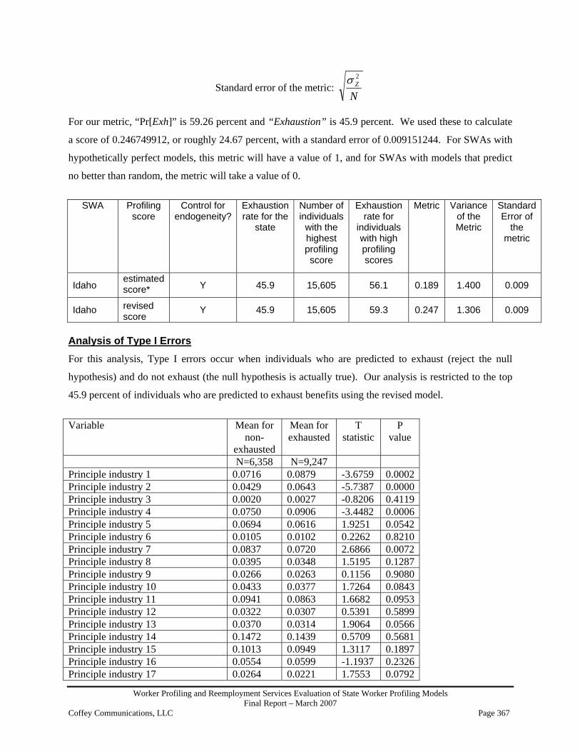
Worker Profiling and Reemployment Services Evaluation of State Worker Profiling Models Final Report – March 2007
Coffey Communications, LLC Page 367
Standard error of the metric: N
Z2σ
For our metric, “Pr[Exh]” is 59.26 percent and “Exhaustion” is 45.9 percent. We used these to calculate
a score of 0.246749912, or roughly 24.67 percent, with a standard error of 0.009151244. For SWAs with
hypothetically perfect models, this metric will have a value of 1, and for SWAs with models that predict
no better than random, the metric will take a value of 0.
SWA Profiling
score Control for
endogeneity? Exhaustion rate for the
state
Number of individuals
with the highest profiling score
Exhaustion rate for
individuals with high profiling scores
Metric Variance of the Metric
Standard Error of
the metric
Idaho estimated score* Y 45.9 15,605 56.1 0.189 1.400 0.009
Idaho revised score
Y 45.9 15,605 59.3 0.247 1.306 0.009
Analysis of Type I Errors For this analysis, Type I errors occur when individuals who are predicted to exhaust (reject the null
hypothesis) and do not exhaust (the null hypothesis is actually true). Our analysis is restricted to the top
45.9 percent of individuals who are predicted to exhaust benefits using the revised model.
Variable Mean for
non- exhausted
Mean for exhausted
T statistic
P value
N=6,358 N=9,247 Principle industry 1 0.0716 0.0879 -3.6759 0.0002 Principle industry 2 0.0429 0.0643 -5.7387 0.0000 Principle industry 3 0.0020 0.0027 -0.8206 0.4119 Principle industry 4 0.0750 0.0906 -3.4482 0.0006 Principle industry 5 0.0694 0.0616 1.9251 0.0542 Principle industry 6 0.0105 0.0102 0.2262 0.8210 Principle industry 7 0.0837 0.0720 2.6866 0.0072 Principle industry 8 0.0395 0.0348 1.5195 0.1287 Principle industry 9 0.0266 0.0263 0.1156 0.9080 Principle industry 10 0.0433 0.0377 1.7264 0.0843 Principle industry 11 0.0941 0.0863 1.6682 0.0953 Principle industry 12 0.0322 0.0307 0.5391 0.5899 Principle industry 13 0.0370 0.0314 1.9064 0.0566 Principle industry 14 0.1472 0.1439 0.5709 0.5681 Principle industry 15 0.1013 0.0949 1.3117 0.1897 Principle industry 16 0.0554 0.0599 -1.1937 0.2326 Principle industry 17 0.0264 0.0221 1.7553 0.0792

Worker Profiling and Reemployment Services Evaluation of State Worker Profiling Models Final Report – March 2007
Coffey Communications, LLC Page 368
Principle industry 18 0.0417 0.0423 -0.1848 0.8534 County 1 0.2888 0.2571 4.3872 0.0000 County 3 0.0060 0.0062 -0.1479 0.8824 County 5 0.0554 0.0587 -0.8865 0.3753 County 7 0.0044 0.0072 -2.2426 0.0249 County 9 0.0077 0.0103 -1.6477 0.0994 County 11 0.0134 0.0109 1.3837 0.1665 County 13 0.0131 0.0125 0.2789 0.7803 County 15 0.0038 0.0037 0.0987 0.9213 County 17 0.0302 0.0316 -0.4884 0.6252 County 19 0.0278 0.0248 1.1853 0.2359 County 21 0.0112 0.0151 -2.1117 0.0347 County 23 0.0028 0.0022 0.8321 0.4053 County 25 0.0005 0.0006 -0.4525 0.6509 County 27 0.1522 0.1506 0.2750 0.7833 County 29 0.0063 0.0064 -0.0689 0.9451 County 31 0.0236 0.0215 0.8600 0.3898 County 33 0.0005 0.0006 -0.4525 0.6509 County 35 0.0041 0.0052 -0.9842 0.3251 County 37 0.0020 0.0023 -0.2979 0.7658 County 39 0.0107 0.0107 -0.0066 0.9948 County 41 0.0013 0.0012 0.1209 0.9038 County 43 0.0047 0.0053 -0.5021 0.6156 County 45 0.0083 0.0084 -0.0667 0.9468 County 47 0.0069 0.0080 -0.7667 0.4432 County 49 0.0126 0.0119 0.3844 0.7007 County 51 0.0038 0.0037 0.0987 0.9213 County 53 0.0099 0.0101 -0.0916 0.9270 County 55 0.0942 0.1012 -1.4448 0.1485 County 57 0.0066 0.0062 0.3414 0.7328 County 59 0.0049 0.0066 -1.3798 0.1677 County 61 0.0008 0.0008 0.0651 0.9481 County 63 0.0014 0.0024 -1.3283 0.1841 County 65 0.0017 0.0015 0.3316 0.7402 County 67 0.0260 0.0293 -1.2497 0.2114 County 69 0.0266 0.0249 0.6641 0.5067 County 71 0.0006 0.0009 -0.5226 0.6013 County 73 0.0013 0.0014 -0.2471 0.8048 County 75 0.0142 0.0156 -0.7157 0.4742 County 77 0.0050 0.0075 -1.8592 0.0630 County 79 0.0190 0.0262 -2.9079 0.0036 County 81 0.0019 0.0017 0.2278 0.8198 County 83 0.0406 0.0430 -0.7531 0.4514 County 85 0.0052 0.0042 0.8810 0.3783 County 87 0.0107 0.0099 0.4545 0.6495 RATIO 2.5162 2.2665 19.7311 0.0000 Total benefit amount 4273.8606 3771.4340 13.8354 0.0000 Job tenure 44.1269 38.4212 4.9044 0.0000 Number of employers 1.7364 1.7698 -1.9374 0.0527

Worker Profiling and Reemployment Services Evaluation of State Worker Profiling Models Final Report – March 2007
Coffey Communications, LLC Page 369
Marital status 0.5340 0.5371 -0.3907 0.6961 January filing 0.1316 0.1466 -2.6491 0.0081 February filing 0.1000 0.0864 2.8947 0.0038 March filing 0.0700 0.0700 0.0053 0.9958 April filing 0.1175 0.1208 -0.6257 0.5315 May filing 0.0595 0.0517 2.0921 0.0364 June filing 0.0827 0.0682 3.3961 0.0007 July filing 0.0643 0.0635 0.2130 0.8313 August filing 0.0590 0.0547 1.1330 0.2572 September filing 0.0728 0.0621 2.6490 0.0081 October filing 0.0931 0.0971 -0.8357 0.4033 November filing 0.1118 0.1351 -4.3073 0.0000 December filing 0.0376 0.0438 -1.9156 0.0554 Number of years of education 12.6711 12.3802 6.6890 0.0000 For the above table, 9,247 individuals exhausted benefits and 6,358 did not. The total of these two types
of individuals is 15,605, which is 45.9 percent of the 33,997 individuals in the sample. The Type I
analysis shows that certain variables have more explanatory power than others for explaining the
difference between Type I errors and correct predictions. For example, industry 1, county 1, ratio, total
benefit amount, job tenure, and number of years of education have different means for exhaustees and
non-exhaustees.

Worker Profiling and Reemployment Services Evaluation of State Worker Profiling Models Final Report – March 2007
Coffey Communications, LLC Page 370
Expanded Analyses of New Jersey Profiling Data

Worker Profiling and Reemployment Services Evaluation of State Worker Profiling Models Final Report – March 2007
Coffey Communications, LLC Page 371
Analysis of New Jersey Profiling Data
Reported Profiling Model New Jersey uses a logistical regression model to determine claimant’s Worker Profiling and
Reemployment Services (WPRS) eligibility. The model was last revised effective January 1, 2004.
Our first step in analyzing both the model used by and the data provided by New Jersey was to use the
profiling scores provided to produce a decile table as shown below. The decile means in this table are
calculated by dividing the percentage of recipients that exhaust benefits for a given decile by 100. For
example, in the first decile our mean is 0.4994117, or approximately 49.9 percent, which indicates that
approximately 50 percent of benefit recipients in this decile exhausted benefits.
Decile Mean Standard Error (Mean) 1 .4994117 .0037426 2 .5670739 .0037091 3 .5924552 .0036845 4 .6079857 .0036509 5 .6290051 .0036219 6 .6438648 .0035828 7 .6527864 .0035666 8 .6694806 .003529 9 .6911517 .0034598 10 .6901045 .0034657 Total .6242945 .0011471
After creating this decile table, we attempted to replicate these scores using the provided data and
coefficients for the variables given. From the given data, we were able to derive variables and categories
for college graduate, job tenure, recall status, weekly benefit rate, benefit year earnings, county
unemployment rate, and binary variables for occupation categories, and a variable indicating missing data
for occupation. We were able to generate a profiling score that correlated with the given score at .956.
New Jersey did include a binary variable indicating whether or not benefit recipients were selected for
reemployment services. This variable will allow us to test for endogeneity within our data and answer the
question - does referral to re-employment services have an effect on the exhaustion of benefits? To test
for endogeneity, we first calculated the logistic regression model where only score (and a constant) is
used to predict exhaustion.

Worker Profiling and Reemployment Services Evaluation of State Worker Profiling Models Final Report – March 2007
Coffey Communications, LLC Page 372
To test for endogeneity, we first calculated the logistic regression model where only score (and a
constant) is used to predict the probability of benefit exhaustion, Pr[exh].
Logistic Regression Model with score only Logistic regression Number of obs = 178246 LR chi2(1) = 2353.13 Prob > chi2 = 0.0000 Log likelihood = -116808.48 Pseudo R2 = 0.0100 exhaust Coef. Std. Err. z P>z [95% Conf. Interval] score 3.084558 .064866 47.55 0.000 2.957423 3.211693 _cons -1.153446 .0351185 -32.84 0.000 -1.222277 -1.084615 Adding the variable for selection tests for a uniform referral effect. Logistic Regression Model with score and referral Logistic regression Number of obs = 178246 LR chi2(2) = 2381.96 Prob > chi2 = 0.0000 Log likelihood = -116794.07
Pseudo R2 = 0.0101
exhaust Coef. Std. Err. z P>z [95% Conf. Interval] score 3.260315 .0727566 44.81 0.000 3.117715 3.402916 select -.0752425 .0139987 -5.37 0.000 -.1026794 -.0478055 _cons -1.233274 .0381789 -32.30 0.000 -1.308103 -1.158444 The addition of the variable “select” improves the log likelihood from -116,808.48to -116,794.07. The
difference in log likelihood is about 14, which is significant. We next add an interaction term (referral X
score) to test for a non-uniform or unsigned effect.
Logistic Regression Model with score, selection and an interaction term Logistic regression Number of obs = 178246 LR chi2(3) = 2462.44 Prob > chi2 = 0.0000 Log likelihood = -116753.83 Pseudo R2 = 0.0104 exhaust Coef. Std. Err. z P>z [95% Conf. Interval] score 3.618609 .0833604 43.41 0.000 3.455225 3.781992 select .8298088 .1014635 8.18 0.000 .630944 1.028674 xrefscore -1.541696 .1710449 -9.01 0.000 -1.876938 -1.206454 _cons -1.419276 .0436068 -32.55 0.000 -1.504744 -1.333808

Worker Profiling and Reemployment Services Evaluation of State Worker Profiling Models Final Report – March 2007
Coffey Communications, LLC Page 373
Again, the addition of the interaction term changes the log likelihood from -116,794.07to -116,753.83.
The difference in log likelihood is about 40, which is also significant. This analysis shows an unsigned or
non-uniform effect.
The offset variable is calculated from the referral and interaction variables times their coefficients as: .8298088*select - 1.541696*xrefscore This value represents the difference between the Pr[exh] for referred and non-referred individuals.
Adding this variable to the logistic regression model as a fixed coefficient variable should adjust referred
and exempted individuals to the Pr[exh] that they would have had if they were not referred.
By adjusting the original scores with this control for endogeneity, we can estimate the true exhaustion rate
for the original score. The logistic regression has exhaustion as a dependent variable, with score as the
independent variable and the offset, named endoofst, to control for endogeneity.
Logistic regression Number of obs = 178246 Wald chi2(1) = 3153.80 Log likelihood = -116753.83
Prob > chi2 = 0.0000
exhaust Coef. Std. Err. z P>z [95% Conf. Interval] score 3.618608 .0644354 56.16 0.000 3.492317 3.744899 _cons -1.419276 .0349129 -40.65 0.000 -1.487704 -1.350848 endoofst (offset) To show the performance of the profiling score, we ordered individuals into deciles and calculated the
exhaustion rate for each decile along with the standard error. This decile table is how we demonstrate the
effectiveness of each model. The decile means are calculated by dividing the percentage of recipients that
exhaust benefits for a given decile by 100. For example, in the first decile our mean is 0.4994117, or
approximately 49.9 percent, which indicates that approximately 50 percent of benefit recipients in this
decile exhausted benefits.
Decile Mean Standard Error (Mean) 1 .4994117 .0037426 2 .5670739 .0037091 3 .5924552 .0036845 4 .6079857 .0036509 5 .6290051 .0036219 6 .6438648 .0035828

Worker Profiling and Reemployment Services Evaluation of State Worker Profiling Models Final Report – March 2007
Coffey Communications, LLC Page 374
7 .6527864 .0035666 8 .6694806 .003529 9 .6911517 .0034598 10 .6901045 .0034657 Total .6242945 .0011471 Updated Profiling Model The updated model has the same form as the model used to predict score, only the coefficients are
generated using 2003 data, and the model includes the offset to control for endogeneity. We also include
diagnostic statistics to show how well the model works, including a classification table that looks at the
top 62.4 percent of cases (because New Jersey has approximately a 62.4 percent exhaustion rate).
We used the same variables we used to replicate the original profiling score. The resulting model is as
follows.
Updated Model Results Logistic regression Number of obs = 178113 Wald chi2(13) = 5225.33Log likelihood = -115528.73 Prob > chi2 = 0.0000 exhaust Coef. Std. Err. z P>z [95% Conf. Interval] colgrad -.2195809 .0139024 -15.79 0.000 -.2468291 -.1923328 tenure .0281326 .0008863 31.74 0.000 .0263955 .0298697 recnum 1.103466 .4861894 2.27 0.023 .1505526 2.05638 wbr .0028689 .0000718 39.94 0.000 .0027281 .0030096 lnbyearn -.5743164 .0118434 -48.49 0.000 -.597529 -.5511037 unemp .0728332 .0041057 17.74 0.000 .0647863 .0808802 mang_adm .102375 .0246968 4.15 0.000 .0539701 .1507799 sales .0670174 .0248367 2.70 0.007 .0183384 .1156965 cler_adm .1609147 .0209298 7.69 0.000 .119893 .2019363 service -.148766 .0235624 -6.31 0.000 -.1949475 -.1025845 agr_for -1.377021 .0405885 -33.93 0.000 -1.456573 -1.297469 cons_prd -.202511 .0169644 -11.94 0.000 -.2357605 -.1692615 ocmisnum .0477212 .0209034 2.28 0.022 .0067513 .0886911 _cons .9018328 .0388581 23.21 0.000 .8256724 .9779932 endoofst (offset) -------- True -------- Classified D ~D Total + 63579 29993 93572 - 47618 36923 84541

Worker Profiling and Reemployment Services Evaluation of State Worker Profiling Models Final Report – March 2007
Coffey Communications, LLC Page 375
Total 111197 66916 178113 Classified + if predicted Pr(D) >= .624True D defined as exhaust != 0 Sensitivity Pr( + D) 57.18% Specificity Pr( -~D) 55.18% Positive predictive value Pr( D +) 67.95% Negative predictive value Pr(~D -) 43.67% False + rate for true ~D Pr( +~D) 44.82% False - rate for true D Pr( - D) 42.82% False + rate for classified + Pr(~D +) 32.05% False - rate for classified - Pr( D -) 56.33% Correctly classified 56.43% number of observations = 178113 area under ROC curve = 0.5913 The decile table for the updated model is as follows: Decile Mean Standard Error (Mean) 1 .4900629 .0037458 2 .5616754 .003718 3 .5835719 .0036939 4 .5846059 .0036925 5 .6087811 .0036569 6 .6176173 .0036414 7 .6467352 .0035816 8 .6689125 .0035263 9 .7070911 .0034101 10 .7740161 .0031339 Total .6243059 .0011475 From the original score to the updated model, there was a significant improvement. The decile gradient,
which ranged from 0.49 to 0.69 for the original model, improved to 0.49 to 0.77 for the updated model.
Revised Model The revised model is similar to the updated model, but we attempted to incorporate more of the
information in the variable set. We include a continuous version of the education variable and second
order terms to capture nonlinear effects. We developed a model with five continuous variables
(education, job tenure, weekly benefit rate, log of base year earnings, and country unemployment rate),

Worker Profiling and Reemployment Services Evaluation of State Worker Profiling Models Final Report – March 2007
Coffey Communications, LLC Page 376
five second order variables, and ten interaction variables (all the interactions between the four continuous
variables). We retained the other variables from the updated model in their original form.
We created the second order variables by first subtracting their mean (centering), and then squaring them.
We created the interaction variables by centering and multiplying the ten second order combinations. The
means for the four continuous variables are shown below.
stats educ tenure wbr lnbyearn unemp mean 12.25601 4.624428 333.1658 3.058695 5.984065 The logistic regression model results for the revised model are as follows. Logistic regression Number of obs = 178113 Wald chi2(28) = 6369.85 Log likelihood = -114755.9
Prob > chi2 = 0.0000
exhaust Coef. Std. Err. z P>z [95% Conf. Interval] educ -.0277699 .0023751 -11.69 0.000 -.0324249 -.0231148 tenure .0235908 .0015362 15.36 0.000 .0205798 .0266017 recnum 1.174978 .4881747 2.41 0.016 .2181727 2.131782 wbr .0019483 .0000817 23.84 0.000 .0017881 .0021085 lnbyearn -.4664727 .0138149 -33.77 0.000 -.4935494 -.4393961 unemp .0903605 .0044758 20.19 0.000 .081588 .099133 mang_adm .0820552 .0248014 3.31 0.001 .0334454 .1306651 sales .0801861 .0249972 3.21 0.001 .0311925 .1291797 cler_adm .1575941 .0211543 7.45 0.000 .1161324 .1990558 service -.126855 .0237714 -5.34 0.000 -.173446 -.0802639 agr_for -1.377801 .0409314 -33.66 0.000 -1.458025 -1.297577 cons_prd -.2016193 .0172503 -11.69 0.000 -.2354292 -.1678094 ocmisnum .0446574 .0211467 2.11 0.035 .0032105 .0861042 xe2 -.0040069 .0002868 -13.97 0.000 -.004569 -.0034448 xt2 -.0001627 .0000741 -2.20 0.028 -.0003078 -.0000175 xw2 -3.94e-06 8.11e-07 -4.86 0.000 -5.53e-06 -2.35e-06 xl2 .3815962 .0181718 21.00 0.000 .3459802 .4172122 xu2 -.0285628 .0030579 -9.34 0.000 -.0345563 -.0225694 xet .0008329 .0002695 3.09 0.002 .0003047 .001361 xew .0000729 .0000233 3.12 0.002 .0000271 .0001186 xel -.0145786 .0035122 -4.15 0.000 -.0214623 -.0076948 xeu .0035905 .0013345 2.69 0.007 .000975 .0062061 xtw -.0000464 .0000142 -3.28 0.001 -.0000741 -.0000186 xtl .0235582 .002272 10.37 0.000 .0191051 .0280113 xtu -.0020638 .0007209 -2.86 0.004 -.0034768 -.0006507 xwl -.0031613 .0002026 -15.61 0.000 -.0035584 -.0027643 xwu .0001053 .00006 1.75 0.079 -.0000123 .0002229 xlu -.0424881 .0100134 -4.24 0.000 -.062114 -.0228622

Worker Profiling and Reemployment Services Evaluation of State Worker Profiling Models Final Report – March 2007
Coffey Communications, LLC Page 377
_cons 1.253384 .0513738 24.40 0.000 1.152694 1.354075 endoofst (offset) Classification Table -------- True -------- Classified D ~D Total + 60669 26747 87416 - 50528 40169 90697 Total 111197 66916 178113 Classified + if predicted Pr(D) >= .624 True D defined as exhaust != 0 Sensitivity Pr( + D) 54.56% Specificity Pr( -~D) 60.03% Positive predictive value
Pr( D +) 69.40%
Negative predictive value
Pr(~D -) 44.29%
False + rate for true ~D
Pr( +~D) 39.97%
False - rate for true D
Pr( - D) 45.44%
False + rate for classified
+ Pr(~D +) 30.60%
False - rate for classified
- Pr( D -) 55.71%
Correctly classified
56.61%
number of observations = 178113 number of covariate patterns = 177834 Pearson chi2(177805) = 178292.65 Prob > chi2 = 0.2066 number of observations = 178113 area under ROC curve = 0.6050 The decile table for the revised model is as follows. Decile Mean Standard Error (Mean) 1 .480631 .0037437 2 .5402279 .0037345
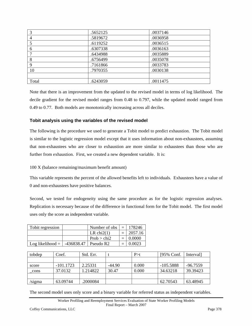
Worker Profiling and Reemployment Services Evaluation of State Worker Profiling Models Final Report – March 2007
Coffey Communications, LLC Page 378
3 .5652125 .0037146 4 .5819672 .0036958 5 .6119252 .0036515 6 .6307338 .0036163 7 .6434988 .0035889 8 .6756499 .0035078 9 .7161866 .0033783 10 .7970355 .0030138 Total .6243059 .0011475 Note that there is an improvement from the updated to the revised model in terms of log likelihood. The
decile gradient for the revised model ranges from 0.48 to 0.797, while the updated model ranged from
0.49 to 0.77. Both models are monotonically increasing across all deciles.
Tobit analysis using the variables of the revised model The following is the procedure we used to generate a Tobit model to predict exhaustion. The Tobit model
is similar to the logistic regression model except that it uses information about non-exhaustees, assuming
that non-exhaustees who are closer to exhaustion are more similar to exhaustees than those who are
further from exhaustion. First, we created a new dependent variable. It is:
100 X (balance remaining/maximum benefit amount) This variable represents the percent of the allowed benefits left to individuals. Exhaustees have a value of
0 and non-exhaustees have positive balances.
Second, we tested for endogeneity using the same procedure as for the logistic regression analyses.
Replication is necessary because of the difference in functional form for the Tobit model. The first model
uses only the score as independent variable.
Tobit regression Number of obs = 178246 LR chi2(1) = 2057.16 Prob > chi2 = 0.0000 Log likelihood = -436838.47 Pseudo R2 = 0.0023 tobdep Coef. Std. Err. t P>t [95% Conf. Interval] score -101.1723 2.25331 -44.90 0.000 -105.5888 -96.7559 _cons 37.0132 1.214822 30.47 0.000 34.63218 39.39423 /sigma 63.09744 .2000084 62.70543 63.48945 The second model uses only score and a binary variable for referred status as independent variables.

Worker Profiling and Reemployment Services Evaluation of State Worker Profiling Models Final Report – March 2007
Coffey Communications, LLC Page 379
Tobit regression Number of obs = 178246 LR chi2(2) = 2085.58 Prob > chi2 = 0.0000 Log likelihood = -436824.26 Pseudo R2 = 0.0024 tobdep Coef. Std. Err. t P>t [95% Conf. Interval] score -107.244 2.527161 -42.44 0.000 -112.1972 -102.2908 select 2.650198 .4968582 5.33 0.000 1.676367 3.624029 _cons 39.76307 1.319853 30.13 0.000 37.17619 42.34995 /sigma 63.09013 .1999825 62.69817 63.48209 The change in log likelihood is about 14, which shows uniform endogeneity. Next is the inclusion of
interaction effects.
Tobit regression Number of obs = 178246 LR chi2(3) = 2160.29 Prob > chi2 = 0.0000 Log likelihood = -436786.9 Pseudo R2 = 0.0025 tobdep Coef. Std. Err. t P>t [95% Conf. Interval] score -119.0531 2.878037 -41.37 0.000 -124.694 -113.4122 select -27.76447 3.54989 -7.82 0.000 -34.72217 -20.80677 xrefscore 51.67789 5.970201 8.66 0.000 39.97643 63.37934 _cons 45.9038 1.499389 30.62 0.000 42.96503 48.84256 /sigma 63.07041 .1999132 62.67859 63.46224 The change in log likelihood is about 38, which again demonstrates endogeneity. The offset variable to
control for endogeneity is:
-27.76447*select + 51.67789*xrefscore The Tobit model uses the same independent variables as the revised model and includes the Tobit control
for endogeneity. The results are as follows.
Tobit regression Number of obs = 178113 LR chi2(28) = 7441.38 Prob > chi2 = 0.0000 Log likelihood = -434168.82 Pseudo R2 = 0.0085 tobdep Coef. Std. Err. t P>t [95% Conf. Interval]
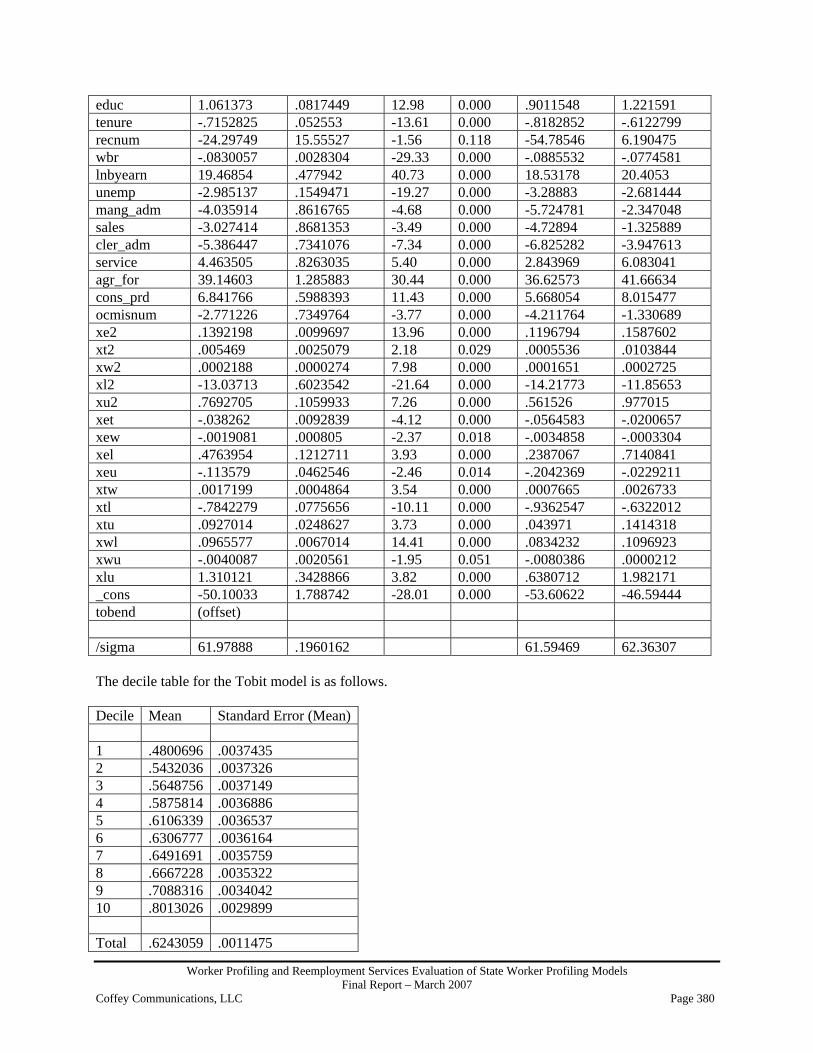
Worker Profiling and Reemployment Services Evaluation of State Worker Profiling Models Final Report – March 2007
Coffey Communications, LLC Page 380
educ 1.061373 .0817449 12.98 0.000 .9011548 1.221591 tenure -.7152825 .052553 -13.61 0.000 -.8182852 -.6122799 recnum -24.29749 15.55527 -1.56 0.118 -54.78546 6.190475 wbr -.0830057 .0028304 -29.33 0.000 -.0885532 -.0774581 lnbyearn 19.46854 .477942 40.73 0.000 18.53178 20.4053 unemp -2.985137 .1549471 -19.27 0.000 -3.28883 -2.681444 mang_adm -4.035914 .8616765 -4.68 0.000 -5.724781 -2.347048 sales -3.027414 .8681353 -3.49 0.000 -4.72894 -1.325889 cler_adm -5.386447 .7341076 -7.34 0.000 -6.825282 -3.947613 service 4.463505 .8263035 5.40 0.000 2.843969 6.083041 agr_for 39.14603 1.285883 30.44 0.000 36.62573 41.66634 cons_prd 6.841766 .5988393 11.43 0.000 5.668054 8.015477 ocmisnum -2.771226 .7349764 -3.77 0.000 -4.211764 -1.330689 xe2 .1392198 .0099697 13.96 0.000 .1196794 .1587602 xt2 .005469 .0025079 2.18 0.029 .0005536 .0103844 xw2 .0002188 .0000274 7.98 0.000 .0001651 .0002725 xl2 -13.03713 .6023542 -21.64 0.000 -14.21773 -11.85653 xu2 .7692705 .1059933 7.26 0.000 .561526 .977015 xet -.038262 .0092839 -4.12 0.000 -.0564583 -.0200657 xew -.0019081 .000805 -2.37 0.018 -.0034858 -.0003304 xel .4763954 .1212711 3.93 0.000 .2387067 .7140841 xeu -.113579 .0462546 -2.46 0.014 -.2042369 -.0229211 xtw .0017199 .0004864 3.54 0.000 .0007665 .0026733 xtl -.7842279 .0775656 -10.11 0.000 -.9362547 -.6322012 xtu .0927014 .0248627 3.73 0.000 .043971 .1414318 xwl .0965577 .0067014 14.41 0.000 .0834232 .1096923 xwu -.0040087 .0020561 -1.95 0.051 -.0080386 .0000212 xlu 1.310121 .3428866 3.82 0.000 .6380712 1.982171 _cons -50.10033 1.788742 -28.01 0.000 -53.60622 -46.59444 tobend (offset) /sigma 61.97888 .1960162 61.59469 62.36307 The decile table for the Tobit model is as follows. Decile Mean Standard Error (Mean) 1 .4800696 .0037435 2 .5432036 .0037326 3 .5648756 .0037149 4 .5875814 .0036886 5 .6106339 .0036537 6 .6306777 .0036164 7 .6491691 .0035759 8 .6667228 .0035322 9 .7088316 .0034042 10 .8013026 .0029899 Total .6243059 .0011475

Worker Profiling and Reemployment Services Evaluation of State Worker Profiling Models Final Report – March 2007
Coffey Communications, LLC Page 381
Note that the Tobit model cannot be compared with the logistic regression models by log likelihood
comparisons. However, from the decile tables, the model appears to be slightly better than the revised
model. It ranges from .48 to .80, while the revised model ranged from .48 to .797
We created a summary table of the four decile tables that allows us to compare models. The Tobit model
allows only marginal improvement over the revised model. The revised model appears to be as good as
any of the other models.
Decile Original
score Adjusted Original score
Updated mean Revised mean Tobit mean
1 .4994117 .4994117 .4900629 .480631 .4800696 2 .5670739 .5670739 .5616754 .5402279 .5432036 3 .5924552 .5924552 .5835719 .5652125 .5648756 4 .6079857 .6079857 .5846059 .5819672 .5875814 5 .6290051 .6290051 .6087811 .6119252 .6106339 6 .6438648 .6438648 .6176173 .6307338 .6306777 7 .6527864 .6527864 .6467352 .6434988 .6491691 8 .6694806 .6694806 .6689125 .6756499 .6667228 9 .6911517 .6911517 .7070911 .7161866 .7088316 10 .6901045 .6901045 .7740161 .7970355 .8013026 Total .6242945 .6242945 .6243059 .6243059 .6243059

Worker Profiling and Reemployment Services Evaluation of State Worker Profiling Models Final Report – March 2007
Coffey Communications, LLC Page 382
New Jersey Profiling Models
0
0.1
0.2
0.3
0.4
0.5
0.6
0.7
0.8
0.9
1 2 3 4 5 6 7 8 9 10
Deciles
Perc
ent o
f ind
ivid
uals
who
exh
aust
ed U
I ben
efits
Original scoreAdjusted original scoreUpdated scoreRevised scoreTobit score
Correlations of the five profiling scores indicate that the updated, revised, and Tobit scores are highly
correlated. The strongest correlation is between the revised and Tobit models with a correlation of .9770.
The original score and adjusted scores are positively correlated with the other three scores, though not at
the same magnitude as the correlation between the other three scores. While the latter three scores are
highly correlated, they are not identical, which suggests that there is a significant difference between the
models.
score prorig prup prrev protobnscore 1.0000 prorig 0.9721 1.0000 prup 0.6670 0.7136 1.0000 prrev 0.5857 0.6293 0.8648 1.0000 protobn 0.5068 0.5478 0.8369 0.9770 1.0000 We also tested the performance of each model using the following metric.
Percent exhausted of the top 62.4 percent of individuals in the score.

Worker Profiling and Reemployment Services Evaluation of State Worker Profiling Models Final Report – March 2007
Coffey Communications, LLC Page 383
We used 62.4 percent because that was the exhaustion rate for benefit recipients in the data set provided
by New Jersey. This metric will vary from about 62.4 percent, for a score that is a random draw, to 100
percent for a score that is a perfect predictor of exhaustion. The scores for the four models are as follows:
Score % exhausted of those with the top 62.4% of score Standard error of the score Original 66.07 .14% Adjusted 66.04 .14% Updated 66.04 .14% Revised 67.58 .14% Tobit 67.46 .14% To compare models across SWAs, we developed a metric to gauge classification improvements between
our models and the original model. In the below metric, “Exhaustion” is the percentage of all benefit
recipients in our sample that exhaust benefits. Here we use 62.4 percent for “Exhaustion” because that
was the exhaustion rate for all benefit recipients for New Jersey. In our metric, “Pr[Exh]” is determined
by the model with the highest percentage of benefit exhaustees with profiling scores falling in the top X
percent of the sample where X percent is determined by the exhaustion rate for all benefit recipients in the
sample. For New Jersey “Pr[Exh]” is represented by the revised model with a score of 71.3 percent for
benefit recipients that exhaust benefits with scores falling in the top 62.4 percent of the score.
In addition to this metric we also applied the equation below, derived by Silverman, Strange, and
Lipscombe (2004), for calculating the variance ( 2zσ ) of a quotient (p. 1069). This equation allowed us to
calculate the variance for our metric, Z = X/Y, which is the quotient of two random variables X (100 -
“Pr[Exh]”) and Y (100 - “Exhaustion”). In the equation below, 2Xσ is the variance of 100 - “Pr[Exh]”,
2Yσ is the variance of 100 - “Exhaustion,” )(XE is the mean for (100 - “Pr[Exh]”), and )(YE is the
mean for (100- “Exhaustion”). By dividing the variance of the quotient of the two random variables
(here 100 - “Exhaustion” and 100 - “Pr[Exh]”) by the square root of our observations we were able to
determine the standard error of the metric.
Metric: Exhaustion
Exh−−
−100
]Pr[1001
Variance of Metric: 4
22
2
22
)()(
)( YEXE
YEYX
zσσ
σ +≈ where X = ( ]Pr[100 Exh− ), (Y = Exhaustion−100 )
Standard error of the metric: N
Z2σ

Worker Profiling and Reemployment Services Evaluation of State Worker Profiling Models Final Report – March 2007
Coffey Communications, LLC Page 384
For our metric we use 67.58 percent for “Pr[Exh]” and 62.4 percent for “Exhaustion” and arrive at a
score of 0.137082369, or roughly 13.7 percent, with a standard error of 0.006008 or 0.65 percent. For
other SWAs, the statistic is recalculated using the exhaustion rate of that SWA from the given sample and
the score from the model with the highest percentage of exhaustion. For SWAs with hypothetically
perfect models, this metric will have a value of 1, and for SWAs with models that predict no better than
random, the metric will take a value of 0.
SWA Profiling
score Control for
endogeneity?Exhaustion rate for the
state
Number of individuals
with the highest profiling score
Exhaustion rate for
individuals with high profiling scores
Metric Variance of the Metric
Standard Error of
the metric
New Jersey
original score
Y 62.4 67,030 66.0 0.096 2.947 0.007
New Jersey
revised score
Y 62.4 67,030 67.6 0.137 2.789 0.006
The above table also shows that the revised score is substantially better than the adjusted score.
Analysis of Type I Errors
Type I errors are individuals who are predicted to exhaust (reject the null hypothesis) and do not exhaust
(the null hypothesis is actually true). Our analysis will be restricted to the top 62.4 percent of individuals
who are predicted to exhaust benefits using the revised model.
Variable Mean for
exhausted Mean for non-
exhausted T
statistic P
value N=75,200 N=36,076 college graduates 0.1014 0.1163 7.5175 0.0000 job tenure 5.4097 5.3742 -0.7663 0.4435 recall status 0.0002 0.0001 -0.9711 0.3315 weekly benefit rate 324.1054 322.8493 -1.6526 0.0984 base year earnings 2.4e+04 2.5e+04 10.8749 0.0000 county unemployment rate 6.2385 6.1882 -6.3755 0.0000 managerial/ administrative 0.0669 0.0671 0.0869 0.9308 sales and related 0.0716 0.0693 -1.4062 0.1597 clerical/administrative support 0.1704 0.1585 -4.9996 0.0000 service occupations 0.0738 0.0754 0.9410 0.3467 agricultural occupations 0.0004 0.0003 -0.2203 0.8256 construction occupations 0.3398 0.3571 5.6879 0.0000 occupation missing 0.1720 0.1697 -0.9467 0.3438

Worker Profiling and Reemployment Services Evaluation of State Worker Profiling Models Final Report – March 2007
Coffey Communications, LLC Page 385
For the table above, note that it includes 75,200 individuals who exhausted benefits and 36,976 who did
not. The total of these two types of individuals is 111,276, which is 62.4 percent of the 178,246
individuals in the sample. The Type I analysis shows that certain variables have more explanatory power
than others for explaining the difference between Type I errors and correct predictions. For example, the
variables for job tenure, recall status, managerial/administrative occupation and agricultural occupation
are not that important for explaining the difference between exhaustees and non-exhaustees. More
important variables, with low p-values, are college graduate, base year earnings, county unemployment
rate, clerical/ administrative support occupation and construction occupation.
References
Silverman, M. P., Strange, W. and Lipscombe, T.C. (2004). The distribution of composite
measurements: How to be certain of the uncertainties in what we measure. American Journal of Physics, 72(8), 1068-1081

Worker Profiling and Reemployment Services Evaluation of State Worker Profiling Models Final Report – March 2007
Coffey Communications, LLC Page 386
Expanded Analyses of Pennsylvania Profiling Data

Worker Profiling and Reemployment Services Evaluation of State Worker Profiling Models Final Report – March 2007
Coffey Communications, LLC Page 387
ANALYSIS OF PENNSYLVANIA PROFILING DATA
Pennsylvania provided its model structure and a dataset for analysis and model revision. Included in this
dataset was a binary variable indicating whether or not benefit recipients were referred to reemployment
services. This binary variable allowed us to test for endogeneity within the data and to answer the
question - does referral to reemployment services have an effect on the exhaustion of benefits?
To test for endogeneity, we first calculated/ran the logistic regression model where only score (and a
constant) was used to predict Pr[exh], their probability of benefit exhaustion.
Logistic Regression Model with score only
Logistic regression Number of observations
= 223906
LR chi2(1) = 1317.60 Prob > chi2 = 0.0000 Log likelihood = -153875.72 Pseudo R2 = 0.0043 exhaust Coefficient Std. Err. Z P>z
[95% Conf.
score 2.592343 .0717106 36.15 0.000 2.451793 2.732894 _cons -1.133801 .0274493 -41.31 0.000 -1.187601 -1.080001 Next, the variables for referral and exempt were added to determine if they increased explanatory power.
The test is a chi-squared test of the difference in the (-2 X log likelihood) statistic for the nested models.
Logistic Regression Model with score, referral, and exempt
Logistic regression Number of observations
= 223906
LR chi2(3) = 3314.48 Prob > chi2 = 0.0000 Log likelihood = -152877.28
Pseudo R2 = 0.0107
exhaust Coefficient Standard
error z P>z [95% Conf. Interval]
score 2.835601 .0806119 35.18 0.000 2.677605 2.993598 refnex .1078473 .0117285 9.20 0.000 .0848599 .1308348 exempt -.7580491 .0192067 -39.47 0.000 -.7956935 -.7204046 _cons -1.201052 .0296161 -40.55 0.000 -1.259098 -1.143005

Worker Profiling and Reemployment Services Evaluation of State Worker Profiling Models Final Report – March 2007
Coffey Communications, LLC Page 388
The addition of the variables “refnex” and “exempt” improves the log likelihood from -153,875.72 to -
152,877.28. This represents a significant difference, showing signed or uniform DIF. Now, we add two
interaction terms (referral-not-exempt X score, and exempt X score) to test for non-uniform or unsigned
DIF.
Logistic Regression Model with score, referral-not-exempt, exempt and their interactions
Logistic regression Number of observations = 223906 LR chi2(5) = 3357.87 Prob > chi2 = 0.0000 Log likelihood = -152855.59 Pseudo R2 = 0.0109 exhaust Coefficient Standard
error z P>z [95% Conf. Interval]
score 3.126434 .0948357 32.97 0.000 2.940559 3.312308 refnex .4218879 .0828933 5.09 0.000 .25942 .5843558 exempt .0027421 .1330698 0.02 0.984 -.2580698 .263554 xexrfnesco -.784345 .2004544 -3.91 0.000 -1.177228 -.3914616 xexsco -1.857989 .3193107 -5.82 0.000 -2.483827 -1.232152 _cons -1.306397 .0347128 -37.63 0.000 -1.374433 -1.238361 Again, the addition of the interaction term changes the log likelihood from -152,877.28 to -152,855.59.
This represents a significant difference, showing unsigned or non-uniform DIF. The coefficients suggest
that the difference between the referred and non-referred individuals is similar to that shown in Figure 3.
For the exempt individuals, the difference is near zero when score is near 0, but with higher levels of
score, exempt individuals have lower-than-expected probability of exhausting UI benefits.
Our proposed remedy is to include a variable in the model with a fixed coefficient that controls for the
referral and exempt effect. This variable, called an offset variable, or offset, will account for the
deviation from the “score - Pr[exhaust]” curve for individuals who are referred or exempted. The value of
this variable is derived from the coefficients of the above regression as:
offset = .4218879*refnex+.0027421*exempt-.784345*xexrfnesco-1.857989*xexsco
This value represents the difference between the Pr[exh] for referred and non-referred, and exempt and
non-exempt individuals. Adding this variable to the logistic regression as a fixed coefficient variable was
done to adjust referred and exempted individuals to the Pr[exh] that they would have had if they were not
referred or exempted.
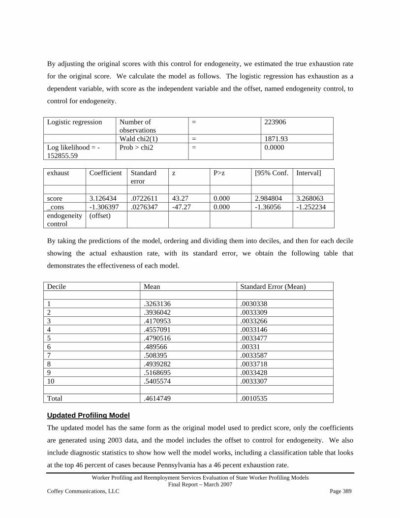
Worker Profiling and Reemployment Services Evaluation of State Worker Profiling Models Final Report – March 2007
Coffey Communications, LLC Page 389
By adjusting the original scores with this control for endogeneity, we estimated the true exhaustion rate
for the original score. We calculate the model as follows. The logistic regression has exhaustion as a
dependent variable, with score as the independent variable and the offset, named endogeneity control, to
control for endogeneity.
Logistic regression Number of
observations = 223906
Wald chi2(1) = 1871.93 Log likelihood = -152855.59
Prob > chi2 = 0.0000
exhaust Coefficient Standard
error z P>z [95% Conf. Interval]
score 3.126434 .0722611 43.27 0.000 2.984804 3.268063 _cons -1.306397 .0276347 -47.27 0.000 -1.36056 -1.252234 endogeneity control
(offset)
By taking the predictions of the model, ordering and dividing them into deciles, and then for each decile
showing the actual exhaustion rate, with its standard error, we obtain the following table that
demonstrates the effectiveness of each model.
Decile Mean Standard Error (Mean) 1 .3263136 .0030338 2 .3936042 .0033309 3 .4170953 .0033266 4 .4557091 .0033146 5 .4790516 .0033477 6 .489566 .00331 7 .508395 .0033587 8 .4939282 .0033718 9 .5168695 .0033428 10 .5405574 .0033307 Total .4614749 .0010535 Updated Profiling Model The updated model has the same form as the original model used to predict score, only the coefficients
are generated using 2003 data, and the model includes the offset to control for endogeneity. We also
include diagnostic statistics to show how well the model works, including a classification table that looks
at the top 46 percent of cases because Pennsylvania has a 46 pecent exhaustion rate.

Worker Profiling and Reemployment Services Evaluation of State Worker Profiling Models Final Report – March 2007
Coffey Communications, LLC Page 390
Updated Model Results
Logistic regression Number of observations = 223906 Wald chi2(8) = 3538.16Log likelihood = -151990.66 Prob > chi2 = 0.0000 exhaust Coefficient Standard error z P>z [95% Conf. Interval] tenind -.1888852 .0088276 -21.40 0.000 -.2061869 -.1715834 eduind1 -.0925952 .013493 -6.86 0.000 -.1190411 -.0661494 eduind2 .0701369 .0124953 5.61 0.000 .0456464 .0946273 decind -.3323059 .0237736 -13.98 0.000 -.3789014 -.2857104 lowrr -.0484037 .016271 -2.97 0.003 -.0802944 -.0165131 hibrr -.0031713 .078394 -0.04 0.968 -.1568208 .1504781 indexh 4.083298 .077704 52.55 0.000 3.931001 4.235595 tur -.0314385 .0043355 -7.25 0.000 -.039936 -.022941 _cons -1.597222 .0422489 -37.81 0.000 -1.680028 -1.514415 endogeneity control (offset) Classification Table
Classified D ~D Total + 63492 60436 123928 - 39835 60143 99978 Total 103327 120579 223906 Classified + if predicted Pr(D) >= .46 True D defined as exhaust != 0 Sensitivity Pr( + D) 61.45% Specificity Pr( -~D) 49.88% Positive predictive value Pr( D +) 51.23% Negative predictive value Pr(~D -) 60.16% False + rate for true ~D Pr( +~D) 50.12% False - rate for true D Pr( - D) 38.55% False + rate for classified + Pr(~D +) 48.77% False - rate for classified - Pr( D -) 39.84% Correctly classified 55.22% Logistic model for exhaust, goodness-of-fit test
number of observations = 223906 number of covariate patterns = 2228 Pearson chi2(2219) = 6861.56 Prob > chi2 = 0.0000

Worker Profiling and Reemployment Services Evaluation of State Worker Profiling Models Final Report – March 2007
Coffey Communications, LLC Page 391
number of observations = 223906 area under ROC curve = 0.5833 The decile table for the updated model is as follows: Decile Mean Standard Error (Mean) 1 .3122766 .0029876 2 .3623209 .0032684 3 .4295011 .0033629 4 .4502674 .0033355 5 .4760161 .0033377 6 .4844848 .0033322 7 .4891484 .003344 8 .5214427 .0033458 9 .528713 .0033358 10 .5674903 .0033117 Total .4614749 .0010535 Revised Model The revised model is the same as the updated model except that seven more variables were added to
account for nonlinear and second order interaction effects.
Logistic regression Number of
observations = 223906
Wald chi2(15) = 4102.60 Log likelihood = -151684.36
Prob > chi2 = 0.0000
exhaust Coefficient Standard
error z P>z [95% Conf. Interval]
tenind -.1868556 .0088761 -21.05 0.000 -.2042524 -.1694588 eduind1 -.0968022 .0135224 -7.16 0.000 -.1233056 -.0702987 eduind2 .0675245 .0125174 5.39 0.000 .0429909 .0920581 decind -.0815156 .0383682 -2.12 0.034 -.156716 -.0063152 lowrr -.0599267 .0163153 -3.67 0.000 -.0919041 -.0279493 hibrr -.0258075 .078488 -0.33 0.742 -.1796411 .1280261 indexh 5.015172 .1268003 39.55 0.000 4.766648 5.263696 tur -.0423947 .0069549 -6.10 0.000 -.0560259 -.0287634 xit -.2096412 .0774124 -2.71 0.007 -.3613667 -.0579157 xid -3.772136 .5402018 -6.98 0.000 -4.830912 -2.71336 xtd .0116573 .0223247 0.52 0.602 -.0320982 .0554129 xiten -1.996344 .1574447 -12.68 0.000 -2.30493 -1.687758 xtten .0253426 .0089136 2.84 0.004 .0078723 .042813 xi2 -15.11698 1.167127 -12.95 0.000 -17.4045 -12.82945 xt2 -.0209703 .0017147 -12.23 0.000 -.024331 -.0176096

Worker Profiling and Reemployment Services Evaluation of State Worker Profiling Models Final Report – March 2007
Coffey Communications, LLC Page 392
_cons -1.873164 .0681795 -27.47 0.000 -2.006793 -1.739535 endogeneity control
(offset)
Classification Table
-------- True -------- Classified D ~D Total + 73578 71064 144642 - 29749 49515 79264 Total 103327 120579 223906 Classified + if predicted Pr(D) >= .46 True D defined as exhaust != 0 Sensitivity Pr( + D) 71.21% Specificity Pr( -~D) 41.06% Positive predictive value
Pr( D +) 50.87%
Negative predictive value
Pr(~D -) 62.47%
False + rate for true ~D
Pr( +~D) 58.94%
False - rate for true D
Pr( - D) 28.79%
False + rate for classified
+ Pr(~D +) 49.13%
False - rate for classified
- Pr( D -) 37.53%
Correctly classified
54.98%
Logistic model for exhaust, goodness-of-fit test number of observations = 223906 number of covariate patterns = 2228 Pearson chi2(2212) = 6360.96 Prob > chi2 = 0.0000 Logistic model for exhaust
number of observations = 223906 area under ROC curve = 0.5879

Worker Profiling and Reemployment Services Evaluation of State Worker Profiling Models Final Report – March 2007
Coffey Communications, LLC Page 393
The decile table for the revised model is as follows. Decile Mean Standard Error (Mean) 1 .2835068 .003012 2 .3783363 .0032347 3 .4261983 .0032915 4 .4586336 .003244 5 .4701638 .0034389 6 .4902339 .003346 7 .4876519 .0033224 8 .5153135 .0031217 9 .5333196 .0035789 10 .577338 .0033472 Total .4614749 .0010535 Tobit Analysis Using the Variables of the Revised Model The procedure that follows was used to generate a Tobit model to predict exhaustion. The Tobit model is
similar to the logit model except that Tobit uses information about non-exhaustees, assuming that non-
exhaustees who are closer to exhaustion are more similar to exhaustees than those claimants who are
further from exhaustion. First, we created a new dependent variable, “/sigma.”
/sigma = 100 X (allowed benefits – benefits paid)/ allowed benefits
This variable represents the percent of the allowed benefits still available to individuals. Exhaustees have
a value of 0. In the data, all negative values were recoded as 0.
Second, we tested for endogeneity using the same procedure as for the logit analyses. Replication is
necessary because of the difference in functional form for the Tobit model. The first model uses only the
score as independent variable.
Tobit regression Number of
observations = 223906
LR chi2(1) = 889.02 Prob > chi2 = 0.0000 Log likelihood = -733011.31 Pseudo R2 = 0.0006 exhvpct Coefficient Standard
error t P>t [95% Conf. Interval]
score -63.35571 2.127225 -29.78 0.000 -67.52502 -59.1864

Worker Profiling and Reemployment Services Evaluation of State Worker Profiling Models Final Report – March 2007
Coffey Communications, LLC Page 394
_cons 32.6816 .8095355 40.37 0.000 31.09494 34.26827 /sigma 55.3712 .1261599 55.12393 55.61847 The second model uses only score, exempt, and referred-not-exempt as independent variables.
Tobit regression Number of
observations = 223906
LR chi2(3) = 3311.91 Prob > chi2 = 0.0000 Log likelihood = -731799.87 Pseudo R2 = 0.0023 exhvpct Coefficient Standard
error t P>t [95% Conf. Interval]
Score -67.55848 2.356731 -28.67 0.000 -72.17761 -62.93935 Refnex -4.896999 .3538844 -13.84 0.000 -5.590604 -4.203395 exempt 22.36194 .5177387 43.19 0.000 21.34718 23.37669 _cons 33.83465 .8611289 39.29 0.000 32.14685 35.52244 /sigma 55.0079 .125249 54.76241 55.25338 The change in log likelihood shows uniform endogeneity. Next is the inclusion of interaction effects.
Tobit regression Number of
observations = 223906
LR chi2(5) = 3395.68 Prob > chi2 = 0.0000 Log likelihood = -731757.98 Pseudo R2 = 0.0023 exhvpct Coefficient Standard
error t P>t [95% Conf. Interval]
Score -76.39179 2.778797 -27.49 0.000 -81.83816 -70.94542 Refnex -9.065158 2.480393 -3.65 0.000 -13.92666 -4.203652 exempt -9.452034 3.524107 -2.68 0.007 -16.35919 -2.544873 xexrfnesco 11.17242 6.005183 1.86 0.063 -.5975842 22.94243 Xexsco 77.79561 8.513585 9.14 0.000 61.1092 94.48201 _cons 37.02261 1.011061 36.62 0.000 35.04096 39.00426 /sigma 54.99493 .1252164 54.74951 55.24035 The change in log likelihood again demonstrates endogeneity. The offset variable to control for
endogeneity is:
offset = -9.065158*ref-9.452034*exempt+11.17242*xexrfnesco+77.79561*xexsco

Worker Profiling and Reemployment Services Evaluation of State Worker Profiling Models Final Report – March 2007
Coffey Communications, LLC Page 395
The Tobit model uses the same independent variables as the revised model and includes the control for
endogeneity.
Tobit regression Number of observations = 223906 LR chi2(15) = 2995.07 Prob > chi2 = 0.0000 Log likelihood = -730963.51 Pseudo R2 = 0.0020 exhvpct Coefficient Standard
error t P>t [95% Conf. Interval]
tenind 4.621223 .2603629 17.75 0.000 4.110919 5.131528 eduind1 3.088008 .3889418 7.94 0.000 2.325692 3.850324 eduind2 -2.403472 .3715285 -6.47 0.000 -3.131658 -1.675285 decind 1.480894 1.11586 1.33 0.184 -.7061634 3.667951 lowrr 1.437 .4829383 2.98 0.003 .4904536 2.383547 hibrr 4.656828 2.261252 2.06 0.039 .2248323 9.088824 indexh -127.455 3.659758 -34.83 0.000 -134.628 -120.282 tur 1.020195 .1998597 5.10 0.000 .6284755 1.411915 xit 13.52186 2.133034 6.34 0.000 9.341166 17.70255 xid 141.3555 15.53334 9.10 0.000 110.9105 171.8004 xtd -1.305497 .6269963 -2.08 0.037 -2.534394 -.0766006 xiten 60.77506 4.471539 13.59 0.000 52.01096 69.53916 xtten -.6976938 .2540387 -2.75 0.006 -1.195603 -.1997845 xi2 266.5333 34.07283 7.82 0.000 199.7514 333.3152 xt2 .5510001 .0475255 11.59 0.000 .4578514 .6441488 _cons 53.83535 1.962353 27.43 0.000 49.98919 57.68151 endogeneity control
(offset)
/sigma 54.75564 .124555 54.51151 54.99976 The decile table for the Tobit model is as follows. Decile Mean Standard Error (Mean) 1 .2820718 .0029993 2 .3851224 .0032586 3 .4253426 .0032817 4 .4496224 .0031531 5 .4794263 .0034658 6 .482314 .003434 7 .5036359 .0031605 8 .5088421 .0034105 9 .5275927 .0034569 10 .5782828 .0033163 Total .4614749 .0010535

Worker Profiling and Reemployment Services Evaluation of State Worker Profiling Models Final Report – March 2007
Coffey Communications, LLC Page 396
We created a summary table of the four decile tables that allows us to compare models. The Tobit model
allows only marginal improvement over the revised model. The revised model is best.
Decile Original score Updated score Revised score Tobit score 1 .3263136 .3122766 .2835068 .28207182 .3936042 .3623209 .3783363 .38512243 .4170953 .4295011 .4261983 .42534264 .4557091 .4502674 .4586336 .44962245 .4790516 .4760161 .4701638 .47942636 .489566 .4844848 .4902339 .4823147 .508395 .4891484 .4876519 .50363598 .4939282 .5214427 .5153135 .50884219 .5168695 .528713 .5333196 .527592710 .5405574 .5674903 .577338 .5782828 Total .4614749 .4614749 .4614749 .4614749
Pennsylvania Comparison of the Models for Calculating Profiling Scores
0
0.1
0.2
0.3
0.4
0.5
0.6
0.7
1 2 3 4 5 6 7 8 9 10
Deciles of Score VAlues
Rat
io fo
Exh
aust
ees
for e
ach
deci
le
original scoresupdated scoresrevised scoresTOBIT scores
Correlations of the four profiling scores indicate that all model scores are positively correlated, as is to be
expected. While the scores are positively correlated, they are not identical, which suggests that there are

Worker Profiling and Reemployment Services Evaluation of State Worker Profiling Models Final Report – March 2007
Coffey Communications, LLC Page 397
differences between the models. Here the strongest correlation exists between the revised and Tobit
models with a correlation of 0.9894.
original score updated score revised score tobit score original score 1.0000 updated score 0.5511 1.0000 revised score 0.5066 0.9463 1.0000 tobit score 0.5080 0.9327 0.9894 1.0000 We also tested the performance of each model using the metric below.
Percent exhausted of the top 46.1 percent of individuals in the score.
We used 46.1 percent because the exhaustion rate for benefit recipients in the Pennsylvania dataset was
46.1 percent. This metric will vary from about 46.1 percent, for a score that is a random draw, up to 100
percent for a score that is a perfect predictor of exhaustion. The scores for the four models are as follows:
Score % exhausted of those with the top 46.1%
of score Standard error of the score
Original 49.33 0.15727 Updated 52.29 0.15493 Revised 52.48 0.15547 Tobit 52.39 0.15542 We note that the revised score performed better than the updated and Tobit scores. The original score
performed worst, and the updated score performed slightly worse than the revised score.
To compare models across SWAs, we developed a metric to gauge classification improvements between
our models and the original model. In the metric below, “Exhaustion” is the percentage of all benefit
recipients in our sample that exhaust benefits. Here we use 46.1 percent for “Exhaustion” because the
exhaustion rate for all benefit recipients for Pennsylvania was 46.1 percent. “Pr[Exh]” in our metric is
determined by the model with the highest percentage of benefit exhaustees with profiling scores falling in
the top X percent, of the sample where X percent is determined by the exhaustion rate for all benefit
recipients in the sample. For Pennsylvania, “Pr[Exh]” is represented by the revised model with a score of
52.48 percent for benefit recipients that exhaust benefits with scores falling in the top 46.1 percent.
In addition to this metric, we also applied the equation below, derived by Silverman, Strange, and
Lipscombe (2004), for calculating the variance ( 2zσ ) of a quotient (p. 1069). This equation allowed us to

Worker Profiling and Reemployment Services Evaluation of State Worker Profiling Models Final Report – March 2007
Coffey Communications, LLC Page 398
calculate the variance for our metric, Z = X/Y, which is the quotient of two random variables X (100 -
“Pr[Exh]”) and Y (100 - “Exhaustion”). In the equation below, 2Xσ is the variance of 100 - “Pr[Exh],”
2Yσ is the variance of 100 - “Exhaustion,” )(XE is the mean for (100 - “Pr[Exh]”), and )(YE is the
mean for (100- “Exhaustion”). By dividing the variance of the quotient of the two random variables
(here 100 - “Exhaustion” and 100 - “Pr[Exh]”) by the square root of our observations we were able to
determine the standard error of the metric.
Metric = 1 – (100 – Pr[Exh])/(100 – Exhaustion)
Variance of Metric: 4
22
2
22
)()(
)( YEXE
YEYX
zσσ
σ +≈ where X = ( ]Pr[100 Exh− ), Y = ( Exhaustion−100 )
Standard error of the metric: N
Z2σ
For our metric, “Pr[Exh]” is 52.48 percent and “Exhaustion” is 46.1 percent. We used these to calculate
a score of 0.1311, or roughly 13.11 percent, with a standard error of 0.004340011. For SWAs with
hypothetically perfect models, this metric will have a value of 1, and for SWAs with models that predict
no better than random, the metric will take a value of 0.
SWA Profiling
score Control for
endogeneity?Exhaustion rate for the
state
Number of individuals
with the highest profiling score
Exhaustion rate for
individuals with high profiling scores
Metric Variance of the Metric
Standard Error of
the metric
Pennsylvania original score
Y 46.1 103,172 51.2 0.095 1.564 0.004
Pennsylvania revised score
Y 46.1 103,172 52.5 0.118 1.527 0.004
Type I Errors Analysis For this analysis, Type I errors occur when individuals who are predicted to exhaust (reject the null
hypothesis), do not exhaust (the null hypothesis is actually true). The analysis is restricted to the top 46.1
percent of individuals who are predicted to exhaust benefits using the revised model.

Worker Profiling and Reemployment Services Evaluation of State Worker Profiling Models Final Report – March 2007
Coffey Communications, LLC Page 399
Variable Mean for exhausted
Mean for non-
exhausted
T statistic
P value
N=54,154 N=49,018 Tenure with most recent employer 0.4471 0.4022 14.5700 0.0000 Education less than 12 years 0.0640 0.0654 -0.8947 0.3710 Education of 16 or more years 0.2503 0.2346 5.8819 0.0000 Declining industry 0.0254 0.0241 1.3262 0.1848 Low benefit replacement rate 0.1071 0.1054 0.9064 0.3647 High benefit replacement rate 0.0020 0.0017 1.2687 0.2045 Industry exhaustion rate 0.4676 0.4693 -8.1571 0.0000 Total unemployment rate of area 5.5065 5.5039 0.5369 0.5913 For the above table, 54,154 individuals exhausted benefits and 49,018 did not. The total of these two
types of individuals is 103,172, which is 46.1 percent of the 223,906 individuals in the sample. The Type
I analysis shows that certain variables have more explanatory power than others for explaining the
difference between Type I errors and correct predictions. For example, the area unemployment rate, low
education level, and low benefit replacement rate variables are not that important for explaining the
difference between exhaustees and non-exhaustees. More important variables, with low p-values, are
tenure with most recent employer, education – college grad+, and industry exhaustion rate.

Worker Profiling and Reemployment Services Evaluation of State Worker Profiling Models Final Report – March 2007
Coffey Communications, LLC Page 400
Expanded Analyses of Texas Profiling Data

Worker Profiling and Reemployment Services Evaluation of State Worker Profiling Models Final Report – March 2007
Coffey Communications, LLC Page 401
ANALYSIS OF TEXAS PROFILING DATA
Reported Profiling Model Texas uses a statistical model whose functional form is a logistic regression to select individuals for
participation in the WPRS Program. The model was last updated in September 2003 with the North
American Industry Classification System (NAICS) replacing the Standard Industrial Classification (SIC)
system and the Standard Occupational Classification (SOC) system replacing the Dictionary of
Occupational Titles (DOT).
The first step in analyzing both the model used and the data was to order the profiling data into a decile
table as shown below. The decile means (the average for each group representing 10 percent) in this table
are calculated by dividing the percentage of recipients that exhaust Unemployment Insurance (UI)
benefits for a given decile by 100. For example, in the first decile our mean is 0.3120462, or 31.2
percent, which indicates that approximately 31 percent of benefit recipients in this decile exhausted
benefits.
Decile Mean Standard Error (Mean) 1 .3120462 .0023265 2 .3797816 .0024018 3 .4156162 .0024895 4 .4265862 .0024906 5 .4619196 .0025132 6 .4787928 .0024786 7 .5114555 .0025492 8 .5475704 .0024834 9 .596076 .0024753 10 .6780035 .0023531 Total .4803744 .0007935
After creating this decile table, we attempted to replicate these scores using the data and coefficients for
the variables given in the document “Rapid Reemployment Model.” While we were able to identify all
variables from the dataset, two factors limited our ability to replicate the profiling scores. First, there was
no constant provided with the model. To address this, through trial and error of picking constant values,
we estimated a constant for the model of 0.2775. This enabled us to replicate the profiling scores for
most cases. Second, there were 433 cases, out of a sample of 396,447, for which data were missing.
Therefore, our analysis will be based on the 396,014 cases for which we had complete information.

Worker Profiling and Reemployment Services Evaluation of State Worker Profiling Models Final Report – March 2007
Coffey Communications, LLC Page 402
Even for the cases with complete information, our replication of the SWA profiling score was
significantly different from that which the SWA provided. There may be two reasons for this difference.
First, the given coefficients were rounded off to 2 or 3 significant digits. For a model with 19 variables,
this rounding could, in some cases, make a large difference in the estimated profiling score. However,
there remained some cases with large differences. Second, there may be cases for which data were not
accurate. Therefore, we assume that some individuals may have inaccurate information for at least one
variable.
The table below shows the characteristics of the difference between our predicted score and the given
score. The second column shows that 1 percent of the difference on the low side is -0.1109866 or less,
and that 10 percent of the difference on the low side is -0.045519 or less. The 50th percentile, or the
median, differs only by .0001864, which is fairly close. On the high side, 10 percent of the cases have a
difference between actual and replicated profiling score of 0.053146 or greater. On the whole, our ability
to replicate the given profiling score was within about .05 for more than 80 percent of the cases. The
third and fourth columns of the table contain other univariate statistics of the difference variable.
Difference between predicted and given profiling scores
Percentiles 1% -.1109866 5% -.0665765 10% -.045519 Observations 396014 25% -.011548 Sum of Weight 396014 50% .0001864 Mean .0017419 Std. Dev. .0428359 75% .0138439 90% .053146 Variance .0018349 95% .0770493 Skewness .2779308 99% .1318981 Kurtosis 9.56145
Texas included a binary variable indicating whether or not benefit recipients were referred to
reemployment services; therefore, we were able to test for endogeneity within the data regarding whether
referral to reemployment services had an effect on the exhaustion of benefits. We proceeded on the
assumption that the given profiling score is what Texas used in its WPRS referral system for 2003.
To test for endogeneity, we first calculated the logistic regression model where only “score” and a
“constant” are used to predict exhaustion.

Worker Profiling and Reemployment Services Evaluation of State Worker Profiling Models Final Report – March 2007
Coffey Communications, LLC Page 403
Logistic Regression Model with score only
Logistic regression Number of observations
= 396447
LR chi2(1) = 17098.79 Prob > chi2 = 0.0000 Log likelihood = -265941.25 Pseudo R2 = 0.0311 Exhaust Coefficient Standard
error z P>z [95% Conf. Interval]
Score 3.853365 .0303001 127.17 0.000 3.793978 3.912752 _cons -1.995095 .0154028 -129.53 0.000 -2.025284 -1.964906 Adding the variable for “referral” tested for a uniform referral effect. The test is a chi-squared test of
difference in the (-2 X log likelihood) statistic for the nested models.
Logistic Regression Model with score and referral
Logistic regression
Number of observations
= 396447 Logistic regression
LR chi2(2) = 17104.72 Prob > chi2 = 0.0000 Log likelihood = -265938.29
Pseudo R2 = 0.0312 Log likelihood = -265938.29
Exhaust Coefficient Standard
error z P>z [95% Conf. Interval]
Score 3.851421 .0303101 127.07 0.000 3.792014 3.910827 Refer -.0183026 .007518 -2.43 0.015 -.0330376 -.0035677 _cons -1.980377 .016542 -119.72 0.000 -2.012799 -1.947955 The addition of the variable “refer” improves the log likelihood from -265,941.25 to -265,938.29. The
difference in log likelihood is 2.94, and the chi-square test for significance is two times this difference
with one degree of freedom. This analysis shows a significant difference, showing signed or uniform
effect. We added an interaction term (referral X score) to test for a non-uniform or unsigned effect.
Logistic Regression Model with score, referral and an interaction term
Logistic regression Number of observations = 396447 LR chi2(3) = 17120.02 Prob > chi2 = 0.0000 Log likelihood = -265930.64 Pseudo R2 = 0.0312

Worker Profiling and Reemployment Services Evaluation of State Worker Profiling Models Final Report – March 2007
Coffey Communications, LLC Page 404
Exhaust Coefficient Standard
error z P>z [95% Conf. Interval]
Score 4.046741 .058563 69.10 0.000 3.93196 4.161523 Refer .1153608 .0350337 3.29 0.001 .0466961 .1840255 Refer X score
-.2673757 .0684468 -3.91 0.000 -.401529 -.1332224
_cons -2.078348 .0300881 -69.08 0.000 -2.13732 -2.019377 Again, the addition of the interaction term changes the log likelihood from -265,938.29 to -265,930.64.
The difference in log likelihood shows an unsigned or non-uniform effect in addition to the signed effect.
The offset variable is calculated from the referral and interaction variables times their coefficients as:
offset = .1153608*refer - .2673757*score
This value represents the difference between the Pr[exh] for referred and non-referred individuals.
Adding this variable to the logit as a fixed coefficient variable adjusts referred and exempted individuals
to the Pr[exh] that they would have had if they were not referred.
By adjusting the original scores with this control for endogeneity, we estimated the true exhaustion rate
for the original score. The logit regression has exhaustion as a dependent variable, with score as the
independent variable and the offset, named endovar, to control for endogeneity.
Logistic regression Number of
observations = 396447
Wald chi2(1) = 17831.05 Log likelihood = -265930.64
Prob > chi2 = 0.0000
exhaust Coefficient Standard
error z P>z [95% Conf. Interval]
score 4.046741 .0303052 133.53 0.000 3.987344 4.106138 _cons -2.078348 .0154047 -134.92 0.000 -2.108541 -2.048156 endovar (offset) By taking the predictions of the model, ordering and dividing them into deciles, and then for each decile
showing the actual exhaustion rate, with its standard error, we obtain the following table that
demonstrates the effectiveness of each model.

Worker Profiling and Reemployment Services Evaluation of State Worker Profiling Models Final Report – March 2007
Coffey Communications, LLC Page 405
Profiling Means and Standard Error of Means by Decile
Decile Mean Standard Error (Mean) 1 .3129018 .0023235 2 .3784102 .0024286 3 .4162552 .0024553 4 .4261504 .0025116 5 .4616296 .0025031 6 .4794217 .0024943 7 .5101999 .0025307 8 .5468143 .0024918 9 .5970523 .0024683 10 .6775371 .0023529 Total .4803744 .0007935 Updated Profiling Model The updated model has the same form as the model used to predict score, only the coefficients are
generated using 2003 data, and the model includes the offset to control for endogeneity. Diagnostic
statistics are included to show how well the model works, including a classification table that looks at the
top 48 percent of cases because that was Texas’ exhaustion rate.
Updated Model Results
Logistic regression Number of observations = 396014 Wald chi2(19) = 17652.32Log likelihood = -265,658.95 Prob > chi2 = 0.0000 exhaust Coefficient Standard
error z P>z [95% Conf. Interval]
eqwksreg -.0852572 .0008736 -97.60 0.000 -.0869694 -.0835451 tenlong .3735053 .0135625 27.54 0.000 .3469233 .4000874 tenshort -.3614415 .0079099 -45.69 0.000 -.3769446 -.3459384 delay1 .097212 .0086662 11.22 0.000 .0802266 .1141974 delay2 .3870738 .0093073 41.59 0.000 .3688318 .4053158 metbea .1029851 .0072996 14.11 0.000 .0886781 .117292 turm2 5.378269 .1791041 30.03 0.000 5.027232 5.729307 pt .1966226 .0382476 5.14 0.000 .1216585 .2715866 lnaww -.2169386 .0077563 -27.97 0.000 -.2321406 -.2017365 logwba2 .4811158 .0124413 38.67 0.000 .4567314 .5055003 info .2604191 .0197951 13.16 0.000 .2216214 .2992167 manufact .1492092 .0111637 13.37 0.000 .1273287 .1710898 oserv .1453133 .0204281 7.11 0.000 .105275 .1853516 transwre .1062135 .0204164 5.20 0.000 .0661981 .1462289
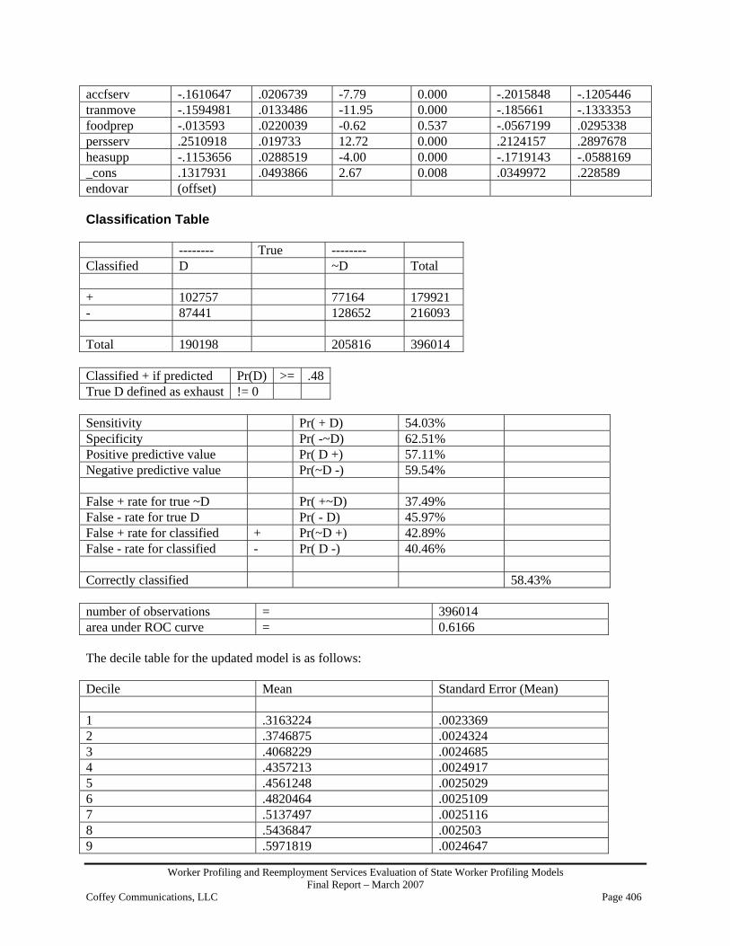
Worker Profiling and Reemployment Services Evaluation of State Worker Profiling Models Final Report – March 2007
Coffey Communications, LLC Page 406
accfserv -.1610647 .0206739 -7.79 0.000 -.2015848 -.1205446 tranmove -.1594981 .0133486 -11.95 0.000 -.185661 -.1333353 foodprep -.013593 .0220039 -0.62 0.537 -.0567199 .0295338 persserv .2510918 .019733 12.72 0.000 .2124157 .2897678 heasupp -.1153656 .0288519 -4.00 0.000 -.1719143 -.0588169 _cons .1317931 .0493866 2.67 0.008 .0349972 .228589 endovar (offset) Classification Table -------- True -------- Classified D ~D Total + 102757 77164 179921 - 87441 128652 216093 Total 190198 205816 396014 Classified + if predicted Pr(D) >= .48True D defined as exhaust != 0 Sensitivity Pr( + D) 54.03% Specificity Pr( -~D) 62.51% Positive predictive value Pr( D +) 57.11% Negative predictive value Pr(~D -) 59.54% False + rate for true ~D Pr( +~D) 37.49% False - rate for true D Pr( - D) 45.97% False + rate for classified + Pr(~D +) 42.89% False - rate for classified - Pr( D -) 40.46% Correctly classified 58.43% number of observations = 396014 area under ROC curve = 0.6166 The decile table for the updated model is as follows: Decile Mean Standard Error (Mean) 1 .3163224 .0023369 2 .3746875 .0024324 3 .4068229 .0024685 4 .4357213 .0024917 5 .4561248 .0025029 6 .4820464 .0025109 7 .5137497 .0025116 8 .5436847 .002503 9 .5971819 .0024647

Worker Profiling and Reemployment Services Evaluation of State Worker Profiling Models Final Report – March 2007
Coffey Communications, LLC Page 407
10 .6764728 .0023509 Total .480281 .0007939 From the original score to the updated model, there was a significant improvement. The decile gradient,
which ranged from a low of 0.31 to a high of 0.68 for the original model, declined slightly to a low of
0.31 to a high of 0.67 for the updated model. Also, the updated model shows a monotonic increase in
ability to predict exhaustion. Thus, decile shows a higher exhaustion rate than the previous one.
Revised Model The revised model is similar to the updated model; it incorporates more of the information in the variable
set. Second-order terms were included to capture nonlinear and discontinuous effects. We made some
changes to limit multicollinearity, thus improving the consistency of the model. The revised model
consists of the following variables.
1) Categorical variables for:
a) Long and short tenure
b) Long and short delay
c) Metroplex region
d) Industry codes indicating employment in information, manufacturing, other services,
transportation and warehousing, or accommodation and food services
e) Occupation codes indicating employment in transportation and moving, food preparation,
personal care and service, and health care support.
2) Binary variable indicating claimant’s need for public transportation
3) Continuous variables for potential duration of benefits, local unemployment rate, natural log of
weekly benefit amount, and a variable for the log of wage replacement rate, which we created
4) Second-order variables for potential duration of benefits and local unemployment rate. Note: The
second-order variables for the natural log of weekly benefit amount and the natural log of wage
replacement rate were collinear and added little new information
5) Five interaction variables for all possible interactions between the continuous variables except for
the interaction between the natural log of weekly benefit amount and wage replacement rate
The second-order was created by first centering the variables, by subtracting their mean, and squaring
them. The interaction variables were created by centering and multiplying the four second-order
combinations. The means for the four continuous variables are shown below.

Worker Profiling and Reemployment Services Evaluation of State Worker Profiling Models Final Report – March 2007
Coffey Communications, LLC Page 408
stats eqwksreg turm2 logwrr logwba2
mean 21.17213 .0659975 -.871123 5.470707
The revised model is as follows:
Logistic regression Number of observations = 396014 Wald chi2(26) = 18380.12Log likelihood = -265,114.54 Prob > chi2 = 0.0000 Exhaust Coefficient Standard
error z P>z [95% Conf. Interval]
eqwksreg -.0709764 .0011989 -59.20 0.000 -.0733263 -.0686265 tenlong .3883972 .013637 28.48 0.000 .3616692 .4151251 tenshort -.3447177 .007934 -43.45 0.000 -.3602681 -.3291674 delay1 .1023993 .0086852 11.79 0.000 .0853766 .1194219 delay2 .3965806 .0093421 42.45 0.000 .3782704 .4148909 metbea .0877413 .0075076 11.69 0.000 .0730268 .1024559 turm2 7.618689 .2540258 29.99 0.000 7.120808 8.11657 pt .182516 .0381749 4.78 0.000 .1076946 .2573374 logwba2 .1762326 .0112668 15.64 0.000 .15415 .1983151 info .2807952 .0198679 14.13 0.000 .2418549 .3197354 manufact .1544734 .0111798 13.82 0.000 .1325614 .1763855 oserv .1311824 .020436 6.42 0.000 .0911287 .1712362 transwre .1032244 .0204489 5.05 0.000 .0631453 .1433036 accfserv -.1608104 .0206414 -7.79 0.000 -.2012668 -.120354 tranmove -.1626694 .0133726 -12.16 0.000 -.1888793 -.1364595 foodprep -.0196018 .0219647 -0.89 0.372 -.0626519 .0234483 persserv .2461699 .0197114 12.49 0.000 .2075363 .2848035 heasupp -.1113396 .0288778 -3.86 0.000 -.167939 -.0547403 eqwks2 .0035772 .0001889 18.94 0.000 .0032069 .0039474 trm2 -75.20079 6.116247 -12.30 0.000 -87.18842 -63.21317 logwrr .2412488 .0085946 28.07 0.000 .2244037 .258094 xeqwrr .0258452 .001211 21.34 0.000 .0234716 .0282188 xeqtrm -.3521697 .0386875 -9.10 0.000 -.4279958 -.2763437 xeqlg -.0326464 .0018581 -17.57 0.000 -.0362883 -.0290045 xtrmlg 3.649509 .4233222 8.62 0.000 2.819813 4.479205 xtrmwrr .29173 .4403165 0.66 0.508 -.5712745 1.154734 _cons .163165 .0582598 2.80 0.005 .0489778 .2773521 endovar (offset) Classification Table
-------- True -------- Classified D ~D Total + 100647 73965 174612

Worker Profiling and Reemployment Services Evaluation of State Worker Profiling Models Final Report – March 2007
Coffey Communications, LLC Page 409
- 89551 131851 221402 Total 190198 205816 396014 Classified + if predicted Pr(D) >= .480 True D defined as exhaust != 0 Sensitivity Pr( + D) 52.92% Specificity Pr( -~D) 64.06% Positive predictive value Pr( D +) 57.64% Negative predictive value Pr(~D -) 59.55% False + rate for true ~D Pr( +~D) 35.94% False - rate for true D Pr( - D) 47.08% False + rate for classified + Pr(~D +) 42.36% False - rate for classified - Pr( D -) 40.45% Correctly classified 58.71% number of observations = 396014 area under ROC curve = 0.6205 The decile table for the revised model is as follows. Decile Mean Standard Error (Mean) 1 .3085955 .0023212 2 .3679107 .0024233 3 .4043585 .0024662 4 .434484 .0024909 5 .4634984 .0025059 6 .4860361 .0025116 7 .5137244 .0025116 8 .5428009 .0025033 9 .5986465 .0024632 10 .6827605 .0023387 Total .480281 .0007939 Note that there is an improvement from the updated to the revised model in terms of log likelihood.
However, the decile gradient for the revised model and the updated model shows only minimal
difference. Both models are monotonically increasing across all deciles.
Tobit analysis using the variables of the revised model The following procedure was used to generate a Tobit model to predict exhaustion. The Tobit model is
similar to the logit model except that it uses information about non-exhaustees, assuming that non-

Worker Profiling and Reemployment Services Evaluation of State Worker Profiling Models Final Report – March 2007
Coffey Communications, LLC Page 410
exhaustees who are closer to exhaustion are more similar to exhaustees than those who are further from
exhaustion. First, we created a new dependent variable, “/sigma.”
/sigma = 100 X (maximum benefit amount – benefits paid)/ maximum benefit amount
This variable represents the percent of the allowed benefits left to individuals. Exhaustees have a value of
0. In the data, all negative values were recoded as 0.
Second, we tested for endogeneity using the same procedure as for the logit analyses. Replication is
necessary because of the difference in functional form for the Tobit model. The first model uses only the
score as independent variable.
Tobit regression Number of observations = 396447 LR chi2(1) = 18351.92 Prob > chi2 = 0.0000 Log likelihood = -1274342.8 Pseudo R2 = 0.0071 tobit dependent var.
Coefficient Standard error
t P>t [95% Conf. Interval]
score -129.5669 .9669814 -133.99 0.000 -131.4622 -127.6716 _cons 72.06959 .4800877 150.12 0.000 71.12864 73.01055 /sigma 59.43342 .1038993 59.22978 59.63706 The second model uses only score and a binary variable for referred status as independent variables.
Tobit regression Number of observations = 396447 LR chi2(2) = 18406.41 Prob > chi2 = 0.0000 Log likelihood = -1274315.5 Pseudo R2 = 0.0072 tobit dependent var.
Coefficient Standard error
t P>t [95% Conf. Interval]
score -129.404 .9671306 -133.80 0.000 -131.2996 -127.5085 refer 1.770434 .2398955 7.38 0.000 1.300246 2.240622 _cons 70.66097 .5164904 136.81 0.000 69.64867 71.67328 /sigma 59.42635 .1038864 59.22273 59.62996 The change in log likelihood shows uniform endogeneity. Next is the inclusion of interaction effects.

Worker Profiling and Reemployment Services Evaluation of State Worker Profiling Models Final Report – March 2007
Coffey Communications, LLC Page 411
Tobit regression Number of observations = 396447 LR chi2(3) = 18418.81 Prob > chi2 = 0.0000 Log likelihood = -1274309.3 Pseudo R2 = 0.0072 tobit dependent var.
Coefficient Standard error
t P>t [95% Conf. Interval]
score -134.9548 1.850961 -72.91 0.000 -138.5827 -131.327 refer -1.966589 1.088124 -1.81 0.071 -4.09928 .166101 score X refer
7.603824 2.159826 3.52 0.000 3.37063 11.83702
_cons 73.39708 .9333018 78.64 0.000 71.56784 75.22633 /sigma 59.42583 .1038852 59.22222 59.62945 The change in log likelihood again demonstrates endogeneity. The offset variable to control for
endogeneity is:
offset = -1.966589*refer + 7.603824*score times refer
The Tobit model uses the same independent variables as the revised model, and includes the Tobit control
for endogeneity. The results are as follows.
Tobit regression Number of
observations = 396014
LR chi2(26) = 20751.32 Prob > chi2 = 0.0000 Log likelihood = -1272661.1 Pseudo R2 = 0.0081 tobit dependent var.
Coefficient Standard error
t P>t [95% Conf. Interval]
eqwksreg 2.405508 .0381114 63.12 0.000 2.330811 2.480205 tenlong -11.99592 .4418282 -27.15 0.000 -12.86189 -11.12995 tenshort 9.246602 .2470913 37.42 0.000 8.76231 9.730894 delay1 -2.797 .2762329 -10.13 0.000 -3.338409 -2.255592 delay2 -12.87464 .3032737 -42.45 0.000 -13.46904 -12.28023 metbea -2.656668 .2392148 -11.11 0.000 -3.125522 -2.187814 turm2 -301.366 7.983454 -37.75 0.000 -317.0133 -285.7186 pt -4.674928 1.243558 -3.76 0.000 -7.112264 -2.237593 logwba2 -8.648269 .3555935 -24.32 0.000 -9.345222 -7.951317 info -9.694697 .6402673 -15.14 0.000 -10.9496 -8.439792 manufact -5.01057 .359218 -13.95 0.000 -5.714626 -4.306513

Worker Profiling and Reemployment Services Evaluation of State Worker Profiling Models Final Report – March 2007
Coffey Communications, LLC Page 412
oserv -4.481407 .6587477 -6.80 0.000 -5.772532 -3.190281 transwre -2.431678 .6551927 -3.71 0.000 -3.715836 -1.14752 accfserv 5.992467 .6511633 9.20 0.000 4.716207 7.268728 tranmove 5.996153 .4232011 14.17 0.000 5.166691 6.825614 foodprep 1.599792 .6980129 2.29 0.022 .2317081 2.967877 persserv -7.556716 .6404074 -11.80 0.000 -8.811895 -6.301537 heasupp 7.073391 .8995265 7.86 0.000 5.310346 8.836437 eqwks2 -.1252639 .0060941 -20.56 0.000 -.137208 -.1133197 trm2 2754.226 195.026 14.12 0.000 2371.981 3136.471 logwrr -5.992173 .2597402 -23.07 0.000 -6.501256 -5.48309 xeqwrr -.6482221 .0378365 -17.13 0.000 -.7223806 -.5740637 xeqtrm 14.74313 1.25252 11.77 0.000 12.28823 17.19803 xeqlg .9918048 .0595822 16.65 0.000 .8750255 1.108584 xtrmlg -136.8592 13.50226 -10.14 0.000 -163.3232 -110.3951 xtrmwrr -16.67146 13.44361 -1.24 0.215 -43.02053 9.67761 _cons 18.69611 1.830804 10.21 0.000 15.10779 22.28443 endogeneity control
(offset)
/sigma 59.36851 .1038132 59.16503 59.57198 The decile table for the Tobit model is as follows.
Decile Mean Standard Error (Mean) 1 .3120549 .0023283 2 .3705621 .0024269 3 .4054191 .0024672 4 .4346607 .002491 5 .4630691 .0025057 6 .48442 .0025113 7 .5099871 .0025121 8 .5421696 .0025036 9 .5953638 .0024665 10 .685109 .0023341 Total .480281 .0007939
Note that the Tobit model cannot be compared with the logit models by log likelihood comparisons.
However, from the decile tables, the model does not appear to be significantly better than the revised
model.
We created a summary table of the four decile tables that allows us to compare models. The Tobit model
allows only marginal improvement over the revised model. The updated or revised model will yield
better results in predicting benefit exhaustion.

Worker Profiling and Reemployment Services Evaluation of State Worker Profiling Models Final Report – March 2007
Coffey Communications, LLC Page 413
Decile Original Score
Original score (Adjusted for Endogeneity)
Updated score Revised score Tobit score
1 .3120462 .3129018 .3163224 .3085955 .31205492 .3797816 .3784102 .3746875 .3679107 .37056213 .4156162 .4162552 .4068229 .4043585 .40541914 .4265862 .4261504 .4357213 .434484 .43466075 .4619196 .4616296 .4561248 .4634984 .46306916 .4787928 .4794217 .4820464 .4860361 .484427 .5114555 .5101999 .5137497 .5137244 .50998718 .5475704 .5468143 .5436847 .5428009 .54216969 .596076 .5970523 .5971819 .5986465 .595363810 .6780035 .6775371 .6764728 .6827605 .685109 Total .4803744 .480281 .480281 .480281 .480281
Comparison of the Models for Calculating Profiling Scores
0
0.1
0.2
0.3
0.4
0.5
0.6
0.7
0.8
1 2 3 4 5 6 7 8 9 10 11
Deciles of score
Exha
ustio
n R
ate
for e
ach
Dec
ile
Original scoreAdjusted Original score Updated meanRevised meanTobit mean
Correlations of the four profiling scores indicate that all model scores are highly correlated. The original
score is highly correlated (positively) with the other three scores. While the latter three scores are highly
correlated, they are not identical, which suggests that there is a significant difference between the models.

Worker Profiling and Reemployment Services Evaluation of State Worker Profiling Models Final Report – March 2007
Coffey Communications, LLC Page 414
original score updated score revised score tobit score original score 1.0000 updated score 0.8977 1.0000 revised score 0.8710 0.9698 1.0000 tobit score 0.8789 0.9677 0.9864 1.0000 Note that the strongest correlation is between the revised and Tobit models with a correlation score of
almost one. As expected, there is also a very strong positive correlation between the updated, revised,
and Tobit models. However, these correlations are not as strong as the relationship between the revised
model and the Tobit model.
We also tested the performance of each model using the metric below.
Percent exhausted of the top 48 percent of individuals in the score.
We used 48 percent because the exhaustion rate for benefit recipients in the Texas dataset was 48 percent.
This metric will vary from about 48 percent, for a score that is a random draw, to 100 percent for a score
that is a perfect predictor of exhaustion. The scores for the four models are as follows:
Score % exhausted of those with the top 48% of score Standard error of the score Original 56.57 0.11353 Updated 56.65 0.11360 Revised 56.87 0.11353 Tobit 56.73 0.11357 We note that the revised score performed better than the updated score. The original score performed
worst, and the updated score performed slightly worse than the revised and Tobit scores.
To compare models across SWAs, we developed a metric to gauge classification improvements between
our models and the original model. In the metric below, “Exhaustion” is the percentage of all benefit
recipients in our sample that exhaust benefits. Here we use 48 percent for “Exhaustion” because the
exhaustion rate for all benefit recipients for Texas was 48 percent. In our metric, “Pr[Exh]” is determined
by the model with the highest percentage of benefit exhaustees with profiling scores falling in the top X
percent of the sample, where X percent is determined by the exhaustion rate for all benefit recipients in
the sample. For Texas, “Pr[Exh]” is represented by the revised model with a score of 56.87 percent for
benefit recipients that exhaust benefits with scores falling in the top 48 percent.

Worker Profiling and Reemployment Services Evaluation of State Worker Profiling Models Final Report – March 2007
Coffey Communications, LLC Page 415
In addition to this metric, we also applied the equation below, derived by Silverman, Strange, and
Lipscombe (2004), for calculating the variance ( 2zσ ) of a quotient (p. 1069). This equation allowed us to
calculate the variance for our metric, Z = X/Y, which is the quotient of two random variables X (100 -
“Pr[Exh]”) and Y (100 - “Exhaustion”). In the equation below, 2Xσ is the variance of 100 - “Pr[Exh],”
2Yσ is the variance of 100 - “Exhaustion,” )(XE is the mean for (100 - “Pr[Exh]”), and )(YE is the
mean for (100- “Exhaustion”). By dividing the variance of the quotient of the two random variables
(here 100 - “Exhaustion” and 100 - “Pr[Exh]”) by the square root of our observations we were able to
determine the standard error of the metric.
Metric = 1 – (100 – Pr[Exh])/(100 – Exhaustion)
Variance of Metric: 4
22
2
22
)()(
)( YEXE
YEYX
zσσ
σ +≈ , where X = ( ]Pr[100 Exh− ), (Y = Exhaustion−100 )
Standard error of the metric: N
Z2σ
For our metric, “Pr[Exh]” is 56.87 percent and “Exhaustion” is 48 percent. We used these to calculate a
score of 0.169991817, or roughly 17 percent, with a standard error of 0.002849646. For SWAs with
hypothetically perfect models, this metric will have a value of 1, and for SWAs with models that predict
no better than random, the metric will take a value of 0.
SWA Profiling
score Control for
endogeneity?Exhaustion rate for the
state
Number of individuals
with the highest profiling score
Exhaustion rate for
individuals with high profiling scores
Metric Variance of the Metric
Standard Error of
the metric
Texas original score
Y 48.0 190,270 56.6 0.165 1.555 0.003
Texas revised score
Y 48.0 190,270 56.9 0.170 1.545 0.003
Analysis of Type I Errors For this analysis, Type I errors occur when individuals who are predicted to exhaust (reject the null
hypothesis) and do not exhaust (the null hypothesis is actually true). The analysis is restricted to the top
48 percent of individuals who are predicted to exhaust benefits using the revised model.

Worker Profiling and Reemployment Services Evaluation of State Worker Profiling Models Final Report – March 2007
Coffey Communications, LLC Page 416
Variable Mean for
exhausted Mean for non-
exhausted T
statistic P
value N = 108,222 N = 82,073 Potential Duration 17.7026 18.6265 38.0622 0.0000 Tenure of 10 or more years 0.1106 0.1113 0.4754 0.6345 Tenure of less than one year 0.4733 0.4302 -18.7288 0.0000 Delay of 2-6 weeks 0.1933 0.1987 2.9133 0.0036 Delay of 6 or more weeks 0.2967 0.2516 -21.7987 0.0000 Metroplex economic region 0.3077 0.3113 1.7206 0.0853 Local unemployment rate 0.0703 0.0694 -9.7000 0.0000 Public transportation needed 0.0132 0.0124 -1.6114 0.1071 Average weekly wage (log) 6.1254 6.1241 -0.5200 0.6031 Weekly benefit amount (log) 5.3889 5.3773 -5.8280 0.0000 Information industry sector 0.0386 0.0396 1.1452 0.2521 Manufacturing sector 0.1311 0.1288 -1.4718 0.1411 Other service industry sector 0.0361 0.0361 0.0855 0.9319 Transportation and warehousing industry
0.0334 0.0327 -0.7726 0.4398
Accommodation and food services industry
0.0258 0.0288 3.9985 0.0001
Transportation and moving occupations
0.0608 0.0619 1.0084 0.3133
Food preparation occupations 0.0278 0.0291 1.6694 0.0950 Personal care and service occupations 0.0474 0.0490 1.5937 0.1110 Healthcare support occupations 0.0090 0.0080 -2.2022 0.0277 For the above table, 108,222 individuals exhausted benefits and 82,073 did not. The total of these two
types of individuals is 190,295, which is 48 percent of the 396,447 individuals in the sample. The Type I
analysis shows that certain variables have more explanatory power than others for explaining the
difference between Type I errors and correct predictions. For example, the variables for long tenure,
average weekly wage, and other service industry sector are not that important for explaining the
difference between exhaustees and non-exhaustees. More important variables, with lower p-values, are
potential duration, tenure of less than one year and delay of six or more weeks.

Worker Profiling and Reemployment Services Evaluation of State Worker Profiling Models Final Report – March 2007
Coffey Communications, LLC Page 417
Expanded Analyses of West Virginia Profiling Data

Worker Profiling and Reemployment Services Evaluation of State Worker Profiling Models Final Report – March 2007
Coffey Communications, LLC Page 418
Analysis of West Virginia Data
Our first step was to replicate the given scores using the data and variable coefficients provided for the
model. West Virginia provided data in three separate data sets. The first was for individuals who
received services. The second was for individuals who were profiled but did not receive services, and the
third was individuals who were not profiled. We combined the first two data sets for our analysis of the
effectiveness of the profiling score.
From the given data, we identified and replicated variables and categories for weekly benefit allowance,
wage base, file lag, reopens, occupation code, industry code, education level, month of filing, and other
income. One possible source of data corruption was our construction of the variable file lag, or the
difference between the separation date and the ‘begin benefit’ year date. We found many cases where the
result was less than 0, so we cut all cases where the value was less than -9. We also cut all values that
were greater than 450, as these individuals would not have had an opportunity to monetarily qualify for
UI benefits. In constructing these variables, we noticed that there were 5,136 cases with missing data out
of a total of 34,913 individuals. Our replicated score correlated with the provided score at .87.
We first developed a decile table for the original score. This table shows for each decile the actual
exhaustion rate, with its standard error and allows us to demonstrate the effectiveness of each model. It
is:
Original score deciles mean se(mean) 1 .2116266 .00691322 .2552277 .00738013 .3091898 .00782094 .3562428 .00810515 .37611 .00819976 .4039508 .00830367 .4428531 .00840828 .4696101 .00845169 .4801031 .008454510 .5611923 .0084024 Total .3865895 .0026062 We included a binary variable that indicated whether or not benefit recipients were referred to re-
employment services. This binary variable will allow us to test for endogeneity within our data and will
answer the question - does referral to re-employment services have an effect on the exhaustion of

Worker Profiling and Reemployment Services Evaluation of State Worker Profiling Models Final Report – March 2007
Coffey Communications, LLC Page 419
benefits? To test for endogeneity, we first calculated the logit model where only score (and a constant) is
used to predict Pr[exh].
Logit Model with score only Logistic regression Number of obs = 34913 LR chi2(1) = 1455.34 Prob > chi2 = 0.0000 Log likelihood = -22566.217 Pseudo R2 = 0.0312 sumexhst Coef. Std. Err. z P>z [95% Conf. Interval] pexhprob .0426529 .0011478 37.16 0.000 .0404033 .0449025 _cons -1.968648 .0423624 -46.47 0.000 -2.051676 -1.885619 Adding the variable for referral tests for a uniform referral effect. The test would be a chi-squared test of
difference in the (-2 X log likelihood) statistic for the nested models.
Logit Model with score and referral Logistic regression Number of obs = 34913 LR chi2(2) = 1473.72 Prob > chi2 = 0.0000 Log likelihood = -22557.026
Pseudo R2 = 0.0316
sumexhst Coef. Std. Err. z P>z [95% Conf. Interval] pexhprob .0412903 .001189 34.73 0.000 .0389599 .0436207 ref .114108 .0266666 4.28 0.000 .0618424 .1663736 _cons -2.004697 .0432422 -46.36 0.000 -2.089451 -1.919944 The addition of the variable “ref” improved the log likelihood from -22566.217 to -22557.026. The
difference in log likelihood was significant, which is significant at the .05 level. Our next step was to test
for non-uniform effects. We added an interaction term (referral X score) to test for a non-uniform or
unsigned effect.
Logit Model with score, referral and an interaction term Logistic regression Number of obs = 34913 LR chi2(3) = 1475.07 Prob > chi2 = 0.0000 Log likelihood = -22556.35 Pseudo R2 = 0.0317 sumexhst Coef. Std. Err. z P>z [95% Conf. Interval]

Worker Profiling and Reemployment Services Evaluation of State Worker Profiling Models Final Report – March 2007
Coffey Communications, LLC Page 420
pexhprob .0444177 .0029442 15.09 0.000 .0386471 .0501883 ref .23449 .1070069 2.19 0.028 .0247603 .4442196 scorref -.0037394 .0032179 -1.16 0.245 -.0100464 .0025676 _cons -2.102373 .0946569 -22.21 0.000 -2.287897 -1.916849 The addition of the interaction term changes the log likelihood from -22557.026 to -22556.35. The
difference was not significant. The analysis indicates that there is only a need to control for uniform
endogeneity. The offset variable is as follows:
.114108*ref After correcting for endogeneity, we obtain the following decile table. prorigdec mean se(mean) 1 .2124857 .0069234 2 .25666 .0073937 3 .3070979 .007805 4 .3553009 .0081026 5 .382235 .0082267 6 .3981667 .0082862 7 .4372852 .0083956 8 .4743626 .0084525 9 .4800917 .0084569 10 .5623031 .0083977 Total .3865895 .0026062 Updated Model The updated model for West Virginia uses the same variables as used in the original model to predict the
profiling score, only the coefficients are generated using 2003 data. We also included diagnostic statistics
to show how well the model works, including a classification table that looks at the top 38.7 percent of
cases (because West Virginia had approximately a 38.7 percent exhaustion rate for the sample).
There were two variables dropped from the analysis due to multicollinearity, or that the variation in the
variables was replicated by other variables in the model. One was education level below high school
graduate. The other was NAICS industry 233 to 235. The resulting model was as follows.
Logistic regression Number of obs = 29777 Wald chi2(48) = 2178.28Log likelihood = -18833.247 Prob > chi2 = 0.0000

Worker Profiling and Reemployment Services Evaluation of State Worker Profiling Models Final Report – March 2007
Coffey Communications, LLC Page 421
exhaust Coef. Std. Err. z P>z [95% Conf. Interval] wba .0029882 .0002335 12.80 0.000 .0025305 .003446 wagebase -8.08e-06 1.37e-06 -5.90 0.000 -.0000108 -5.40e-06 ten1 .7436879 .0506253 14.69 0.000 .6444642 .8429115 ten2 .5150458 .0558257 9.23 0.000 .4056294 .6244622 ten3 .5122289 .0402284 12.73 0.000 .4333826 .5910751 ten4 .3701485 .0313851 11.79 0.000 .3086348 .4316622 fillag2 .002649 .000219 12.09 0.000 .0022197 .0030783 reopens -.4928575 .024942 -19.76 0.000 -.541743 -.4439721 soca .3750771 .2404267 1.56 0.119 -.0961505 .8463047 socb .0611577 .2392343 0.26 0.798 -.407733 .5300483 socc .1707481 .2375245 0.72 0.472 -.2947914 .6362876 socd .3442268 .238466 1.44 0.149 -.1231579 .8116115 soce .3127174 .2369227 1.32 0.187 -.1516425 .7770774 socg -.0630185 .2374472 -0.27 0.791 -.5284066 .4023695 soch -.0844695 .2412895 -0.35 0.726 -.5573881 .3884492 soci .0966113 .2373195 0.41 0.684 -.3685264 .5617491 socj -.038083 .2377118 -0.16 0.873 -.5039894 .4278235 socl -1.227142 .2462532 -4.98 0.000 -1.709789 -.7444942 naicsa -.1460809 .2552339 -0.57 0.567 -.6463303 .3541684 naicsb -.5651295 .1669446 -3.39 0.001 -.892335 -.2379241 naicse .0405749 .1642364 0.25 0.805 -.2813226 .3624723 naicsf .1499015 .1648961 0.91 0.363 -.173289 .473092 naicsg -.191624 .1611328 -1.19 0.234 -.5074385 .1241905 naicsh -.2697996 .1747613 -1.54 0.123 -.6123255 .0727262 naicsi .1007729 .2266578 0.44 0.657 -.3434681 .545014 naicsj .2096941 .1720147 1.22 0.223 -.1274486 .5468368 naicsk -.1635723 .1977593 -0.83 0.408 -.5511733 .2240288 naicsl -.2944647 .1610682 -1.83 0.068 -.6101526 .0212232 naicsm -.0740427 .1627558 -0.45 0.649 -.3930381 .2449528 naicsn -.4838695 .1897004 -2.55 0.011 -.8556754 -.1120636 naicso -.432979 .166882 -2.59 0.009 -.7600618 -.1058962 naicsp .0849415 .170601 0.50 0.619 -.2494303 .4193133 naicsq -.3549825 .1800176 -1.97 0.049 -.7078106 -.0021544 naicsr -.206361 .1609367 -1.28 0.200 -.5217911 .1090691 ed2 -.1697102 .0379417 -4.47 0.000 -.2440746 -.0953458 ed3 -.4020231 .0572163 -7.03 0.000 -.5141649 -.2898812 bybmo1 -.0235924 .0539444 -0.44 0.662 -.1293214 .0821366 bybmo2 .0616336 .0605959 1.02 0.309 -.0571322 .1803993 bybmo3 .2367095 .0616057 3.84 0.000 .1159646 .3574545 bybmo4 .3594653 .0607978 5.91 0.000 .2403037 .4786269 bybmo5 .0485156 .0665144 0.73 0.466 -.0818503 .1788814 bybmo6 -.2084052 .0597431 -3.49 0.000 -.3254996 -.0913109 bybmo7 .1857606 .0591185 3.14 0.002 .0698905 .3016306 bybmo8 .1801518 .0615319 2.93 0.003 .0595515 .3007521 bybmo9 .0034562 .0705178 0.05 0.961 -.1347561 .1416685 bybmo10 .252192 .0617218 4.09 0.000 .1312196 .3731645

Worker Profiling and Reemployment Services Evaluation of State Worker Profiling Models Final Report – March 2007
Coffey Communications, LLC Page 422
bybmo11 -.0446778 .0596928 -0.75 0.454 -.1616736 .072318 othintot -1.325398 .1048464 -12.64 0.000 -1.530893 -1.119903 _cons -.926875 .2890298 -3.21 0.001 -1.493363 -.360387 endovar (offset) -------- True -------- Classified D ~D Total + 8621 8101 16722 - 3595 9460 13055 Total 12216 17561 29777 Sensitivity Pr( + D) 70.57% Specificity Pr( -~D) 53.87% Positive predictive value Pr( D +) 51.55% Negative predictive value Pr(~D -) 72.46% False + rate for true ~D Pr( +~D) 46.13% False - rate for true D Pr( - D) 29.43% False + rate for classified + Pr(~D +) 48.45% False - rate for classified - Pr( D -) 27.54% Correctly classified 60.72% number of observations = 29777 area under ROC curve = 0.6721 The decile table for the updated model is as follows: prupdec mean se(mean) 1 .175957 .0069789 2 .2437878 .0078693 3 .2971793 .0083761 4 .3399395 .0086831 5 .3895232 .0089374 6 .4308261 .0090758 7 .4662412 .0091445 8 .5238415 .0091535 9 .5815984 .009041 10 .6536782 .0087218 Total .4102495 .0028505
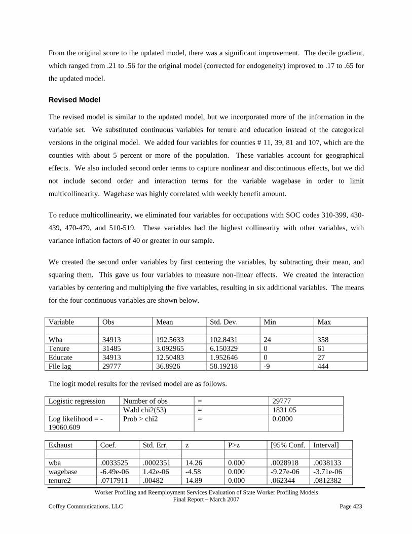
Worker Profiling and Reemployment Services Evaluation of State Worker Profiling Models Final Report – March 2007
Coffey Communications, LLC Page 423
From the original score to the updated model, there was a significant improvement. The decile gradient,
which ranged from .21 to .56 for the original model (corrected for endogeneity) improved to .17 to .65 for
the updated model.
Revised Model The revised model is similar to the updated model, but we incorporated more of the information in the
variable set. We substituted continuous variables for tenure and education instead of the categorical
versions in the original model. We added four variables for counties # 11, 39, 81 and 107, which are the
counties with about 5 percent or more of the population. These variables account for geographical
effects. We also included second order terms to capture nonlinear and discontinuous effects, but we did
not include second order and interaction terms for the variable wagebase in order to limit
multicollinearity. Wagebase was highly correlated with weekly benefit amount.
To reduce multicollinearity, we eliminated four variables for occupations with SOC codes 310-399, 430-
439, 470-479, and 510-519. These variables had the highest collinearity with other variables, with
variance inflation factors of 40 or greater in our sample.
We created the second order variables by first centering the variables, by subtracting their mean, and
squaring them. This gave us four variables to measure non-linear effects. We created the interaction
variables by centering and multiplying the five variables, resulting in six additional variables. The means
for the four continuous variables are shown below.
Variable Obs Mean Std. Dev. Min Max Wba 34913 192.5633 102.8431 24 358 Tenure 31485 3.092965 6.150329 0 61 Educate 34913 12.50483 1.952646 0 27 File lag 29777 36.8926 58.19218 -9 444 The logit model results for the revised model are as follows. Logistic regression Number of obs = 29777 Wald chi2(53) = 1831.05 Log likelihood = -19060.609
Prob > chi2 = 0.0000
Exhaust Coef. Std. Err. z P>z [95% Conf. Interval] wba .0033525 .0002351 14.26 0.000 .0028918 .0038133 wagebase -6.49e-06 1.42e-06 -4.58 0.000 -9.27e-06 -3.71e-06 tenure2 .0717911 .00482 14.89 0.000 .062344 .0812382

Worker Profiling and Reemployment Services Evaluation of State Worker Profiling Models Final Report – March 2007
Coffey Communications, LLC Page 424
fillag2 .0053138 .0004182 12.71 0.000 .0044943 .0061334 educate -.0436911 .0077132 -5.66 0.000 -.0588087 -.0285736 soca .2276896 .0532177 4.28 0.000 .1233848 .3319944 socb -.0969952 .0482557 -2.01 0.044 -.1915747 -.0024157 socd .2300526 .0444252 5.18 0.000 .1429809 .3171244 soch -.2289532 .0583534 -3.92 0.000 -.3433238 -.1145825 socj -.2019862 .0427502 -4.72 0.000 -.2857751 -.1181973 socl -1.372821 .0764903 -17.95 0.000 -1.522739 -1.222903 naicsa -.1696616 .2482049 -0.68 0.494 -.6561343 .3168111 naicsb -.6009846 .1656591 -3.63 0.000 -.9256704 -.2762987 naicse .0091071 .1626834 0.06 0.955 -.3097466 .3279607 naicsf .1616165 .1630974 0.99 0.322 -.1580485 .4812814 naicsg -.1036812 .159973 -0.65 0.517 -.4172226 .2098602 naicsh -.2544863 .1732963 -1.47 0.142 -.5941408 .0851683 naicsi .1865665 .2251364 0.83 0.407 -.2546928 .6278257 naicsj .3354638 .1710194 1.96 0.050 .0002719 .6706556 naicsk -.0798549 .1964173 -0.41 0.684 -.4648258 .305116 naicsl -.2160792 .1598408 -1.35 0.176 -.5293614 .0972031 naicsm .0169084 .1612332 0.10 0.916 -.2991029 .3329198 naicsn -.4029611 .1881527 -2.14 0.032 -.7717336 -.0341887 naicso -.3040127 .1653424 -1.84 0.066 -.6280778 .0200525 naicsp .1644536 .1694502 0.97 0.332 -.1676628 .49657 naicsq -.2838175 .1788067 -1.59 0.112 -.6342722 .0666372 naicsr -.2482247 .1595283 -1.56 0.120 -.5608944 .064445 bybmo1 -.0575788 .0537554 -1.07 0.284 -.1629375 .0477799 bybmo2 .037415 .0603838 0.62 0.536 -.080935 .155765 bybmo3 .2128922 .0614294 3.47 0.001 .0924926 .3332917 bybmo4 .3138914 .0604653 5.19 0.000 .1953815 .4324013 bybmo5 -.0035062 .0660587 -0.05 0.958 -.1329789 .1259665 bybmo6 -.204477 .0595692 -3.43 0.001 -.3212306 -.0877235 bybmo7 .1455612 .0589068 2.47 0.013 .0301061 .2610163 bybmo8 .1819153 .0612726 2.97 0.003 .0618232 .3020074 bybmo9 .030705 .0702562 0.44 0.662 -.1069946 .1684046 bybmo10 .2403364 .0614284 3.91 0.000 .1199389 .3607339 bybmo11 -.0183833 .0594613 -0.31 0.757 -.1349252 .0981587 othintot -1.312701 .1084094 -12.11 0.000 -1.52518 -1.100223 cnty11 -.2606691 .0567545 -4.59 0.000 -.3719058 -.1494324 cnty39 .0455275 .0378433 1.20 0.229 -.0286439 .1196989 cnty81 -.032068 .0567446 -0.57 0.572 -.1432855 .0791494 cnty107 .0466289 .0510532 0.91 0.361 -.0534335 .1466914 xten2 -.0018176 .0002334 -7.79 0.000 -.0022752 -.0013601 xwba2 -9.18e-06 1.62e-06 -5.65 0.000 -.0000124 -6.00e-06 xedu2 .001283 .0017081 0.75 0.453 -.0020649 .0046308 xfil2 -.0000155 1.94e-06 -7.97 0.000 -.0000193 -.0000117 xtwba -.0000145 .0000307 -0.47 0.636 -.0000747 .0000457 xtedu -.0015697 .0011548 -1.36 0.174 -.0038332 .0006937 xtfil -.0000953 .0000321 -2.96 0.003 -.0001583 -.0000323 xwbaedu .0000701 .0000722 0.97 0.331 -.0000714 .0002117 xwbafil 6.07e-06 2.30e-06 2.64 0.008 1.57e-06 .0000106
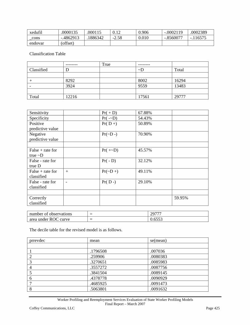
Worker Profiling and Reemployment Services Evaluation of State Worker Profiling Models Final Report – March 2007
Coffey Communications, LLC Page 425
xedufil .0000135 .000115 0.12 0.906 -.0002119 .0002389 _cons -.4862913 .1886342 -2.58 0.010 -.8560077 -.116575 endovar (offset) Classification Table -------- True -------- Classified D ~D Total + 8292 8002 16294 - 3924 9559 13483 Total 12216 17561 29777 Sensitivity Pr( + D) 67.88% Specificity Pr( -~D) 54.43% Positive predictive value
Pr( D +) 50.89%
Negative predictive value
Pr(~D -) 70.90%
False + rate for true ~D
Pr( +~D) 45.57%
False - rate for true D
Pr( - D) 32.12%
False + rate for classified
+ Pr(~D +) 49.11%
False - rate for classified
- Pr( D -) 29.10%
Correctly classified
59.95%
number of observations = 29777 area under ROC curve = 0.6553 The decile table for the revised model is as follows. prrevdec mean se(mean) 1 .1796508 .007036 2 .259906 .0080383 3 .3270651 .0085983 4 .3557272 .0087756 5 .3841504 .0089145 6 .4378778 .0090929 7 .4685925 .0091473 8 .5063801 .0091632

Worker Profiling and Reemployment Services Evaluation of State Worker Profiling Models Final Report – March 2007
Coffey Communications, LLC Page 426
9 .5503694 .0091173 10 .6328519 .008836 Total .4102495 .0028505 This model appears to be similar to the updated model. Tobit analysis using the variables of the revised model For West Virginia, the Tobit analysis is not possible because the total benefit allowance was not provided.
We cannot calculate a dependent variable for the percent of allowable benefits paid.
Summary Tables We created a summary table of the four decile tables that allows us to compare models. To make the
models comparable, we only included cases with full information. For this subsample, the exhaustion
rate is 41 percent, as indicated by the bottom row of the table. While there was considerable
improvement between the adapted and updated models there was no improvement with the revised model.
The updated score appears to be the best model for the data available.
Decile Original
score Original score adapted for endogeneity
Updated score Revised score
1 .2160804 .2135395 .175957 .1796508 2 .2632411 .2686275 .2437878 .259906 3 .3236351 .3225689 .2971793 .3270651 4 .3774373 .3756047 .3399395 .3557272 5 .3924802 .3968833 .3895232 .3841504 6 .4150641 .4106452 .4308261 .4378778 7 .4629278 .4558684 .4662412 .4685925 8 .4799627 .4879032 .5238415 .5063801 9 .4918478 .4909475 .5815984 .5503694 10 .5734245 .5737608 .6536782 .6328519 Total .4102495 .4102495 .4102495 .4102495
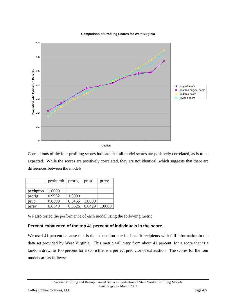
Worker Profiling and Reemployment Services Evaluation of State Worker Profiling Models Final Report – March 2007
Coffey Communications, LLC Page 427
Comparison of Profiling Scores for West Virginia
0
0.1
0.2
0.3
0.4
0.5
0.6
0.7
Deciles
Prop
ortio
n W
ho E
xhau
sted
Ben
efits
original scoreadapted original scoreupdated scorerevised score
Correlations of the four profiling scores indicate that all model scores are positively correlated, as is to be
expected. While the scores are positively correlated, they are not identical, which suggests that there are
differences between the models.
pexhprob prorig prup prrev pexhprob 1.0000 prorig 0.9932 1.0000 prup 0.6399 0.6465 1.0000 prrev 0.6540 0.6626 0.8429 1.0000 We also tested the performance of each model using the following metric. Percent exhausted of the top 41 percent of individuals in the score. We used 41 percent because that is the exhaustion rate for benefit recipients with full information in the
data set provided by West Virginia. This metric will vary from about 41 percent, for a score that is a
random draw, to 100 percent for a score that is a perfect predictor of exhaustion. The scores for the four
models are as follows:

Worker Profiling and Reemployment Services Evaluation of State Worker Profiling Models Final Report – March 2007
Coffey Communications, LLC Page 428
Score % exhausted of those with the top 41% of score Standard error of the score Original .50692 .0045245 Adapted .5070042 .0045252 Updated .5536899 .0044991 Revised .5373904 .0045126 The updated model performs the best. To compare models across SWAs, we developed a metric to gauge classification improvements between
our models and the original model. In the metric below, “Exhaustion” is the percentage of all benefit
recipients in our sample that exhaust benefits. Here we use 41 percent for “Exhaustion” because the
exhaustion rate for all benefit recipients for West Virginia was 41 percent. In our metric, “Pr[Exh]” is
determined by the model with the highest percentage of benefit exhaustees with profiling scores falling in
the top X percent of the sample where X percent is determined by the exhaustion rate for all benefit
recipients in the sample. For West Virginia, “Pr[Exh]” is represented by the updated model with a score
of 55.37 percent for benefit recipients that exhaust benefits with scores falling in the top 41 percent.
In addition to this metric, we also applied the equation below, derived by Silverman, Strange, and
Lipscombe (2004), for calculating the variance ( 2zσ ) of a quotient (p. 1069)iii. This equation allowed us
to calculate the variance for our metric, Z, which is the quotient of two random variables X and Y where
X = 100 - Pr[Exh] and Y = 100 - “Exhaustion.” In the equation below, 2Xσ is the variance of 100 -
Pr[Exh], 2Yσ is the variance of 100 - “Exhaustion,” )(XE is the mean for 100 - Pr[Exh], and )(YE is
the mean for 100 - “Exhaustion.” By dividing the variance of the quotient of the two random variables
(here 100 - “Exhaustion” and 100 - “Pr[Exh]”) by the square root of our observations, we were able to
determine the standard error of the metric.
Metric: ( )Exhaustion
Exh−−
−100
]Pr[1001
Variance of Metric: 4
22
2
22
)()(
)( YEXE
YEYX
zσσ
σ +≈
Standard error of the metric: N
Z2σ
For our metric, we use 55.4 percent for “Pr[Exh]” for the updated model and 50.7 percent for “Pr[Exh]”
for the original adapted model. “Exhaustion” for both was 41 percent. The model metrics are shown
below. For other SWAs, the statistic is recalculated using the exhaustion rate of that SWA from the given
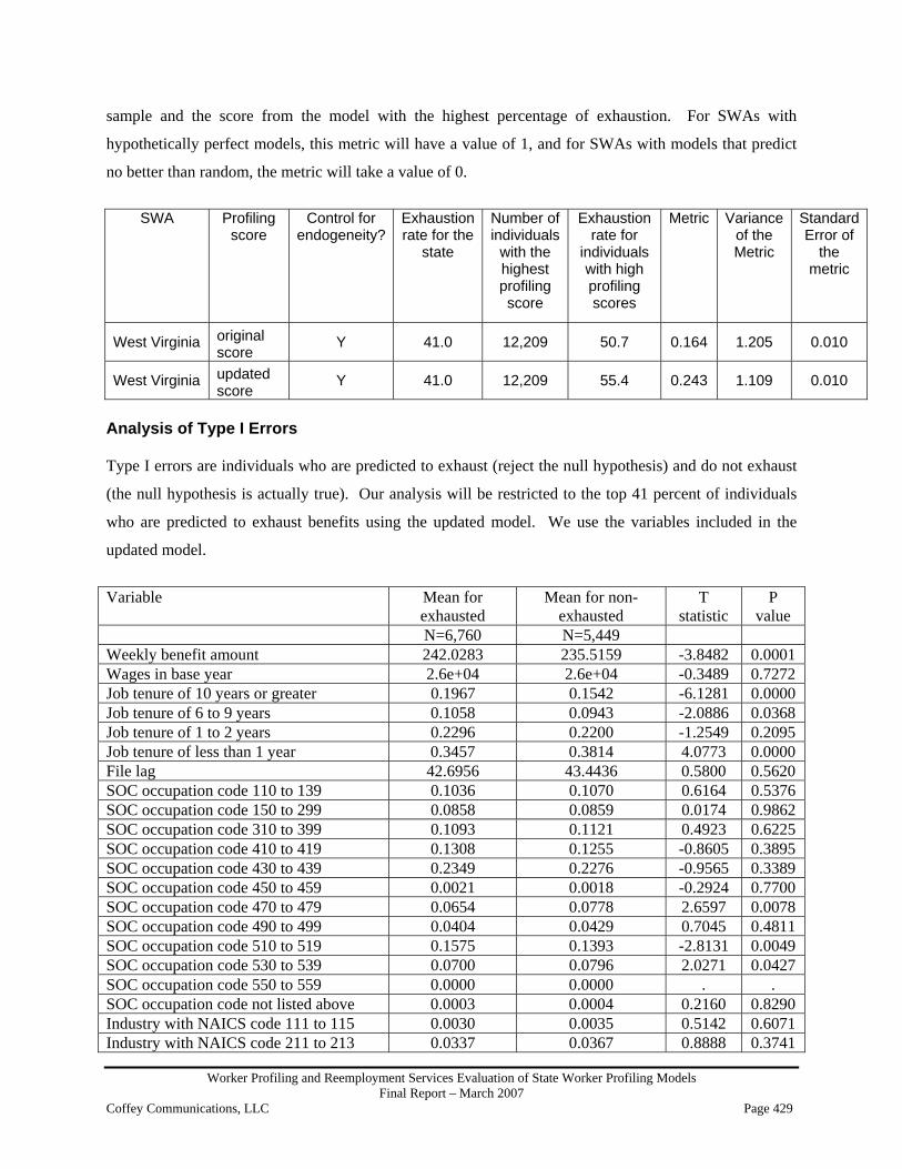
Worker Profiling and Reemployment Services Evaluation of State Worker Profiling Models Final Report – March 2007
Coffey Communications, LLC Page 429
sample and the score from the model with the highest percentage of exhaustion. For SWAs with
hypothetically perfect models, this metric will have a value of 1, and for SWAs with models that predict
no better than random, the metric will take a value of 0.
SWA Profiling
score Control for
endogeneity?Exhaustion rate for the
state
Number of individuals
with the highest profiling score
Exhaustion rate for
individuals with high profiling scores
Metric Variance of the Metric
Standard Error of
the metric
West Virginia original score
Y 41.0 12,209 50.7 0.164 1.205 0.010
West Virginia updated score
Y 41.0 12,209 55.4 0.243 1.109 0.010
Analysis of Type I Errors Type I errors are individuals who are predicted to exhaust (reject the null hypothesis) and do not exhaust
(the null hypothesis is actually true). Our analysis will be restricted to the top 41 percent of individuals
who are predicted to exhaust benefits using the updated model. We use the variables included in the
updated model.
Variable Mean for
exhausted Mean for non-
exhausted T
statistic P
value N=6,760 N=5,449 Weekly benefit amount 242.0283 235.5159 -3.8482 0.0001 Wages in base year 2.6e+04 2.6e+04 -0.3489 0.7272 Job tenure of 10 years or greater 0.1967 0.1542 -6.1281 0.0000 Job tenure of 6 to 9 years 0.1058 0.0943 -2.0886 0.0368 Job tenure of 1 to 2 years 0.2296 0.2200 -1.2549 0.2095 Job tenure of less than 1 year 0.3457 0.3814 4.0773 0.0000 File lag 42.6956 43.4436 0.5800 0.5620 SOC occupation code 110 to 139 0.1036 0.1070 0.6164 0.5376 SOC occupation code 150 to 299 0.0858 0.0859 0.0174 0.9862 SOC occupation code 310 to 399 0.1093 0.1121 0.4923 0.6225 SOC occupation code 410 to 419 0.1308 0.1255 -0.8605 0.3895 SOC occupation code 430 to 439 0.2349 0.2276 -0.9565 0.3389 SOC occupation code 450 to 459 0.0021 0.0018 -0.2924 0.7700 SOC occupation code 470 to 479 0.0654 0.0778 2.6597 0.0078 SOC occupation code 490 to 499 0.0404 0.0429 0.7045 0.4811 SOC occupation code 510 to 519 0.1575 0.1393 -2.8131 0.0049 SOC occupation code 530 to 539 0.0700 0.0796 2.0271 0.0427 SOC occupation code 550 to 559 0.0000 0.0000 . . SOC occupation code not listed above 0.0003 0.0004 0.2160 0.8290 Industry with NAICS code 111 to 115 0.0030 0.0035 0.5142 0.6071 Industry with NAICS code 211 to 213 0.0337 0.0367 0.8888 0.3741
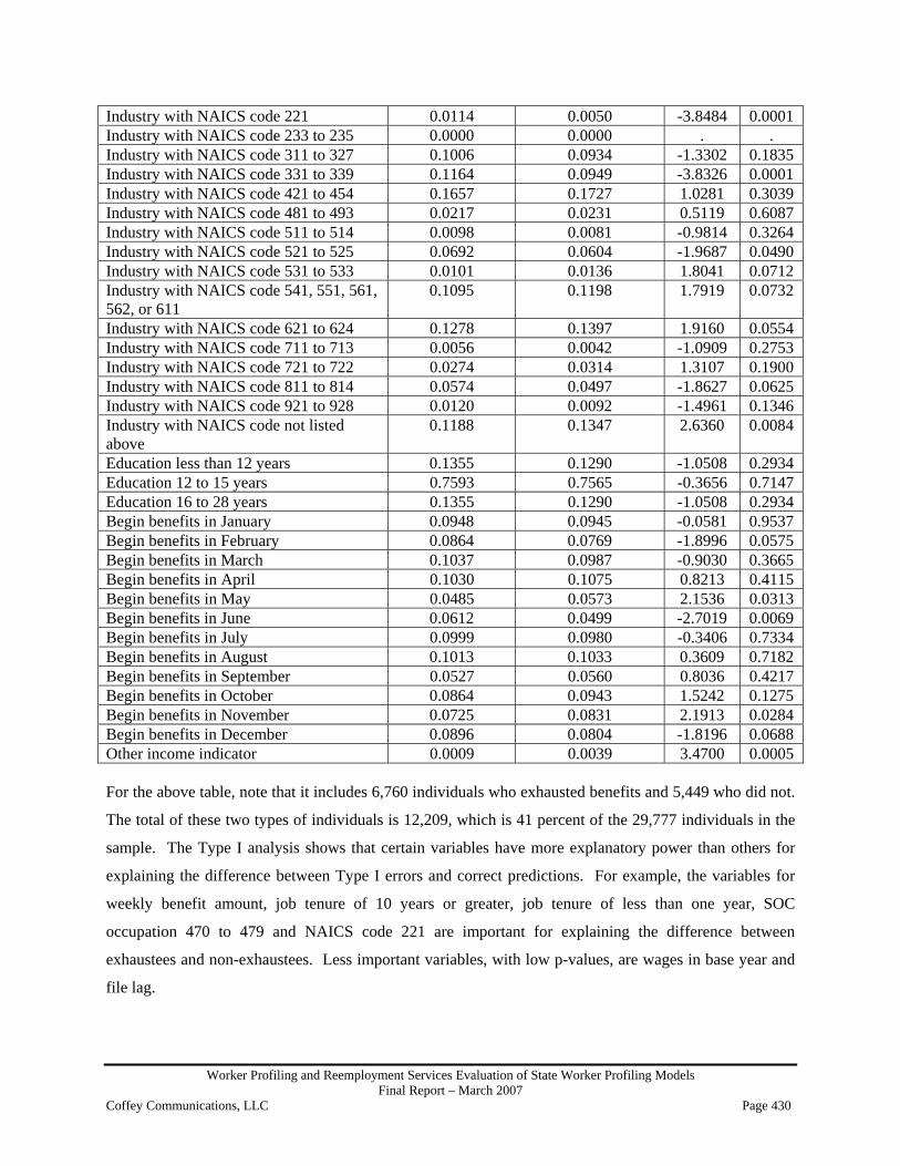
Worker Profiling and Reemployment Services Evaluation of State Worker Profiling Models Final Report – March 2007
Coffey Communications, LLC Page 430
Industry with NAICS code 221 0.0114 0.0050 -3.8484 0.0001 Industry with NAICS code 233 to 235 0.0000 0.0000 . . Industry with NAICS code 311 to 327 0.1006 0.0934 -1.3302 0.1835 Industry with NAICS code 331 to 339 0.1164 0.0949 -3.8326 0.0001 Industry with NAICS code 421 to 454 0.1657 0.1727 1.0281 0.3039 Industry with NAICS code 481 to 493 0.0217 0.0231 0.5119 0.6087 Industry with NAICS code 511 to 514 0.0098 0.0081 -0.9814 0.3264 Industry with NAICS code 521 to 525 0.0692 0.0604 -1.9687 0.0490 Industry with NAICS code 531 to 533 0.0101 0.0136 1.8041 0.0712 Industry with NAICS code 541, 551, 561, 562, or 611
0.1095 0.1198 1.7919 0.0732
Industry with NAICS code 621 to 624 0.1278 0.1397 1.9160 0.0554 Industry with NAICS code 711 to 713 0.0056 0.0042 -1.0909 0.2753 Industry with NAICS code 721 to 722 0.0274 0.0314 1.3107 0.1900 Industry with NAICS code 811 to 814 0.0574 0.0497 -1.8627 0.0625 Industry with NAICS code 921 to 928 0.0120 0.0092 -1.4961 0.1346 Industry with NAICS code not listed above
0.1188 0.1347 2.6360 0.0084
Education less than 12 years 0.1355 0.1290 -1.0508 0.2934 Education 12 to 15 years 0.7593 0.7565 -0.3656 0.7147 Education 16 to 28 years 0.1355 0.1290 -1.0508 0.2934 Begin benefits in January 0.0948 0.0945 -0.0581 0.9537 Begin benefits in February 0.0864 0.0769 -1.8996 0.0575 Begin benefits in March 0.1037 0.0987 -0.9030 0.3665 Begin benefits in April 0.1030 0.1075 0.8213 0.4115 Begin benefits in May 0.0485 0.0573 2.1536 0.0313 Begin benefits in June 0.0612 0.0499 -2.7019 0.0069 Begin benefits in July 0.0999 0.0980 -0.3406 0.7334 Begin benefits in August 0.1013 0.1033 0.3609 0.7182 Begin benefits in September 0.0527 0.0560 0.8036 0.4217 Begin benefits in October 0.0864 0.0943 1.5242 0.1275 Begin benefits in November 0.0725 0.0831 2.1913 0.0284 Begin benefits in December 0.0896 0.0804 -1.8196 0.0688 Other income indicator 0.0009 0.0039 3.4700 0.0005 For the above table, note that it includes 6,760 individuals who exhausted benefits and 5,449 who did not.
The total of these two types of individuals is 12,209, which is 41 percent of the 29,777 individuals in the
sample. The Type I analysis shows that certain variables have more explanatory power than others for
explaining the difference between Type I errors and correct predictions. For example, the variables for
weekly benefit amount, job tenure of 10 years or greater, job tenure of less than one year, SOC
occupation 470 to 479 and NAICS code 221 are important for explaining the difference between
exhaustees and non-exhaustees. Less important variables, with low p-values, are wages in base year and
file lag.

Worker Profiling and Reemployment Services Evaluation of State Worker Profiling Models Final Report – March 2007
Coffey Communications, LLC Page 431
1 Silverman, M. P., Strange, W. and Lipscombe, T.C. (2004). The distribution of composite measurements: How to be certain of the uncertainties in what we measure. American Journal of Physics, 72(8), 1068-1081. 1 Silverman, M. P., Strange, W. and Lipscombe, T.C. (2004). The distribution of composite measurements: How to be certain of the uncertainties in what we measure. American Journal of Physics, 72(8), 1068-1081. 1 Silverman, M. P., Strange, W. and Lipscombe, T.C. (2004). The distribution of composite measurements: How to be certain of the uncertainties in what we measure. American Journal of Physics, 72(8), 1068-1081.