1

Analyzing Social Networks Detailed Instructions on the Examples in the Text This gives the detailed commands required to reproduce all the examples in the text created using UCINET, E-Net and Netdraw. Note we do not show details for Siena or PNet. We are grateful to Daniel Tischer who has documented most of the examples. Occasionally the outputs will not match exactly, this can be for a number of reasons. Some routines use random number generators and the output is dependent on some random number. This may affect the ordering of the output or some values may be different but any differences should be slight. Secondly newer versions of UCINET may have more efficient or later algorithms and this could marginally affect the results but again any differences will be slight. Steve, Martin and Jeff

Contents Section 2.2 Graphs .................................................................................................................................. 4

Section 2.4 Adjacency Matrix.................................................................................................................. 6

Section 5.4.1 Transposing ....................................................................................................................... 8

Section 5.4.5 Combining Relations ....................................................................................................... 10

Section 5.4.6 Combining Nodes ............................................................................................................ 12

Section 5.8 Converting Attributes to Matrices ..................................................................................... 13

Section 5.9 Data Export......................................................................................................................... 14

Section 6.2 Multidimensional Scaling ................................................................................................... 17

Section 6.3 Correspondence Analysis ................................................................................................... 19

Section 6.4 Hierarchical Clustering ....................................................................................................... 21

Section 7.2 Layout ................................................................................................................................. 22

7.2.1 Attribute-based scatter plot: ................................................................................................... 22

7.2.2 Ordination: ............................................................................................................................... 24

7.2.3 Graph layout algorithms .......................................................................................................... 24

Section 7.3 Embedding Node Attributes .............................................................................................. 25

Section 7.4 Node Filtering ..................................................................................................................... 27

Section 7.6 Embedding Tie Characteristics ........................................................................................... 27

7.6.1 Tie Strength .............................................................................................................................. 27

2

7.6.2 Type of tie ................................................................................................................................ 30

Section 7.7 Visualizing Network Change ............................................................................................... 32

Section 8.3 Dyadic Hypothesis .............................................................................................................. 37

QAP Correlation ................................................................................................................................ 37

8.3.1 QAP Regression ........................................................................................................................ 38

Section 8.4 Dyadic-Monadic Hypotheses ............................................................................................. 41

8.4.1 Continuous Attributes .............................................................................................................. 41

8.4.2 Categorical Attributes .............................................................................................................. 42

Section 8.5 Node-level hypothesis ........................................................................................................ 44

Section 9.2 Cohesion ............................................................................................................................. 46

Section 9.3 Reciprocity .......................................................................................................................... 46

Section 10.3 Undirected, Non-valued Networks .................................................................................. 48

10.3.1 Degree Centrality ................................................................................................................... 48

Section 11.2 Cliques .............................................................................................................................. 49

11.2.1 Analyzing clique overlaps ....................................................................................................... 49

11.2.2 Bimodal method .................................................................................................................... 49

11.3 Girvan-Newman Algorithm ........................................................................................................... 50

Section 11.4 Factions and modularity optimization ............................................................................. 51

Section 11.5 Directed and Valued Data ................................................................................................ 53

Section 11.7 Performing a Cohesive Subgraph Analysis ....................................................................... 54

Section 12.3 Profile Similarity ............................................................................................................... 57

Section 12.4 Blockmodels ..................................................................................................................... 59

Section 12.5 The Direct Method ........................................................................................................... 61

Section 12.6 Regular Equivalence ......................................................................................................... 62

Section 12.7 REGE ................................................................................................................................. 63

Section 12.8 Core-Periphery Models .................................................................................................... 64

Section 13.2 Converting to One-Mode Data ......................................................................................... 67

3

Section 13.4 Bipartite Networks ........................................................................................................... 71

Section 13.5 Cohesive Subgroups ......................................................................................................... 72

Section 13.6 Core-Periphery Models .................................................................................................... 74

Section 13.7 Equivalence ...................................................................................................................... 76

Section 14.2 Reducing the Size of the Problem .................................................................................... 79

14.2.4 Aggregation ............................................................................................................................ 80

14.3.1 Using specialized algorithms: ................................................................................................. 81

Section 15.5 Example 2 of an ego network study ................................................................................. 81

4

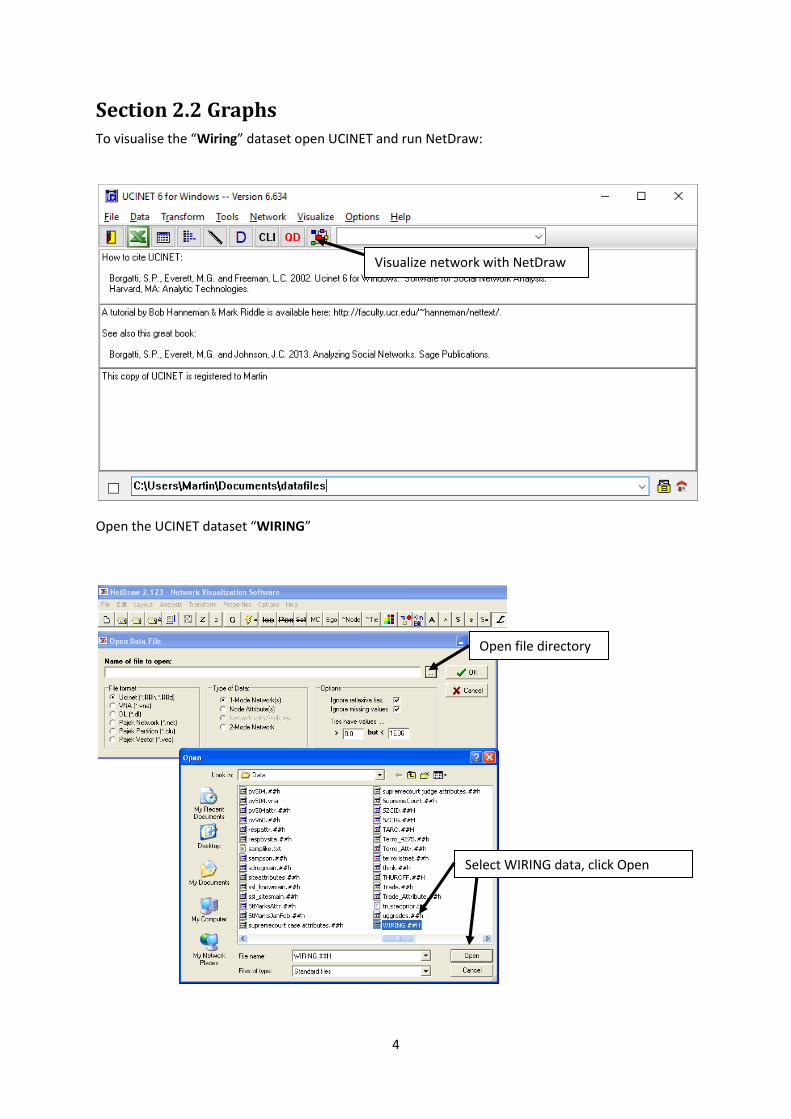
Section 2.2 Graphs To visualise the “Wiring” dataset open UCINET and run NetDraw:

Open the UCINET dataset “WIRING”

Visualize network with NetDraw

Open file directory

Select WIRING data, click Open

5

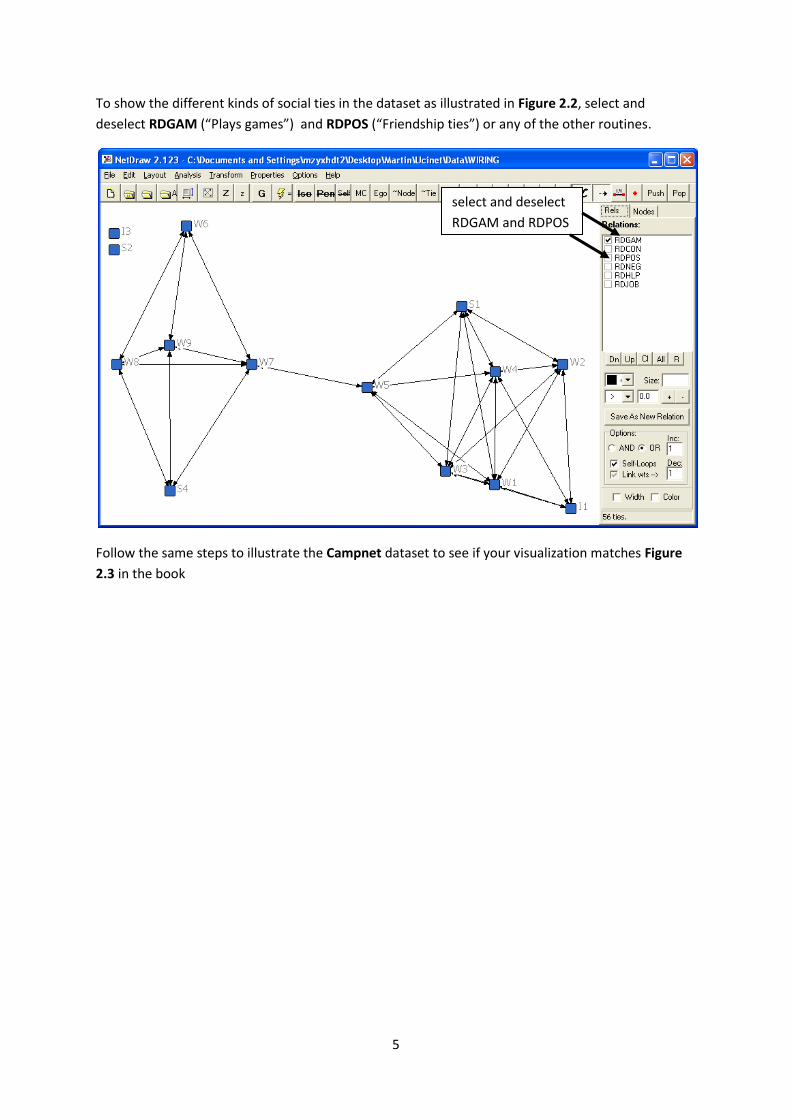
To show the different kinds of social ties in the dataset as illustrated in Figure 2.2, select and

deselect RDGAM (“Plays games”) and RDPOS (“Friendship ties”) or any of the other routines.

Follow the same steps to illustrate the Campnet dataset to see if your visualization matches Figure

2.3 in the book

select and deselect

RDGAM and RDPOS

6

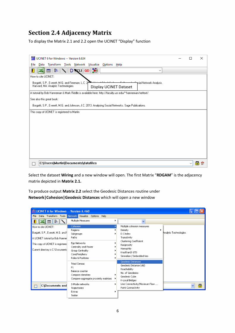
Section 2.4 Adjacency Matrix To display the Matrix 2.1 and 2.2 open the UCINET “Display” function

Select the dataset Wiring and a new window will open. The first Matrix “RDGAM” is the adjacency

matrix depicted in Matrix 2.1.

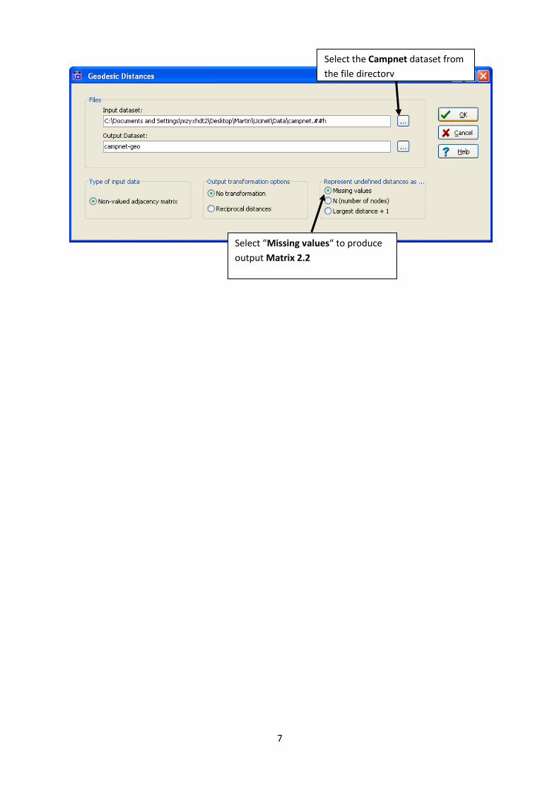
To produce output Matrix 2.2 select the Geodesic Distances routine under

Network|Cohesion|Geodesic Distances which will open a new window

Display UCINET Dataset

7

Select the Campnet dataset from

the file directory

Select “Missing values“ to produce

output Matrix 2.2

8

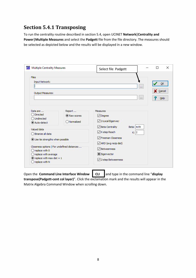
Section 5.4.1 Transposing To run the centrality routine described in section 5.4, open UCINET Network|Centrality and

Power|Multiple Measures and select the Padgett file from the file directory. The measures should

be selected as depicted below and the results will be displayed in a new window.

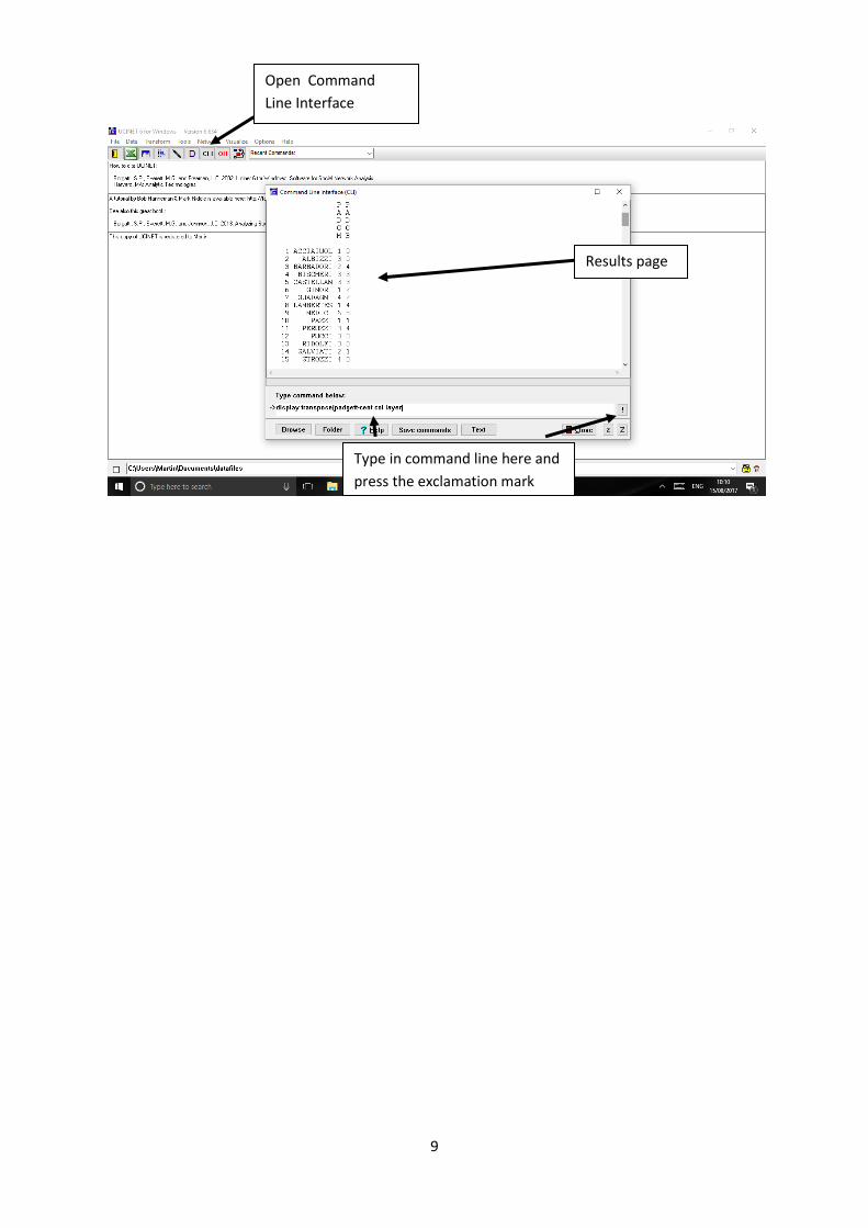
Open the Command Line Interface Window and type in the command line “display

transpose(Padgett-cent col layer)”. Click the exclamation mark and the results will appear in the

Matrix Algebra Command Window when scrolling down.

Select file Padgett

CLI

9

Open Command

Line Interface

Type in command line here and

press the exclamation mark

Results page

10

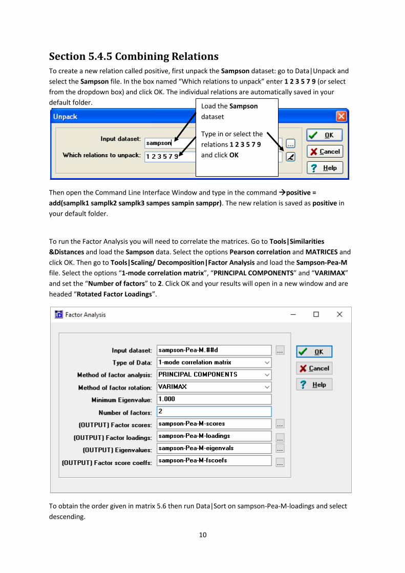
Section 5.4.5 Combining Relations To create a new relation called positive, first unpack the Sampson dataset: go to Data|Unpack and

select the Sampson file. In the box named “Which relations to unpack” enter 1 2 3 5 7 9 (or select

from the dropdown box) and click OK. The individual relations are automatically saved in your

default folder.

Then open the Command Line Interface Window and type in the command positive =

add(samplk1 samplk2 samplk3 sampes sampin samppr). The new relation is saved as positive in

your default folder.

To run the Factor Analysis you will need to correlate the matrices. Go to Tools|Similarities

&Distances and load the Sampson data. Select the options Pearson correlation and MATRICES and

click OK. Then go to Tools|Scaling/ Decomposition|Factor Analysis and load the Sampson-Pea-M

file. Select the options “1-mode correlation matrix”, “PRINCIPAL COMPONENTS” and “VARIMAX”

and set the “Number of factors” to 2. Click OK and your results will open in a new window and are

headed “Rotated Factor Loadings”.

To obtain the order given in matrix 5.6 then run Data|Sort on sampson-Pea-M-loadings and select

descending.

Load the Sampson

dataset

Type in or select the

relations 1 2 3 5 7 9

and click OK

11

12

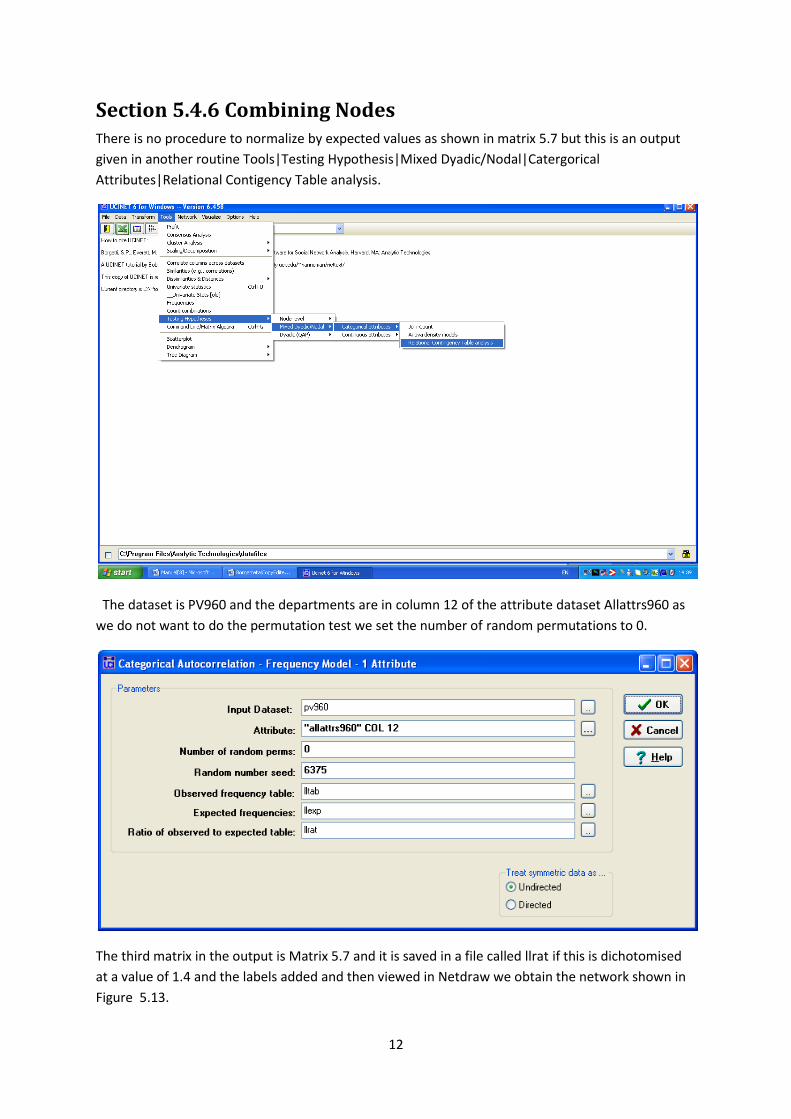
Section 5.4.6 Combining Nodes There is no procedure to normalize by expected values as shown in matrix 5.7 but this is an output

given in another routine Tools|Testing Hypothesis|Mixed Dyadic/Nodal|Catergorical

Attributes|Relational Contigency Table analysis.

The dataset is PV960 and the departments are in column 12 of the attribute dataset Allattrs960 as

we do not want to do the permutation test we set the number of random permutations to 0.

The third matrix in the output is Matrix 5.7 and it is saved in a file called llrat if this is dichotomised

at a value of 1.4 and the labels added and then viewed in Netdraw we obtain the network shown in

Figure 5.13.

13

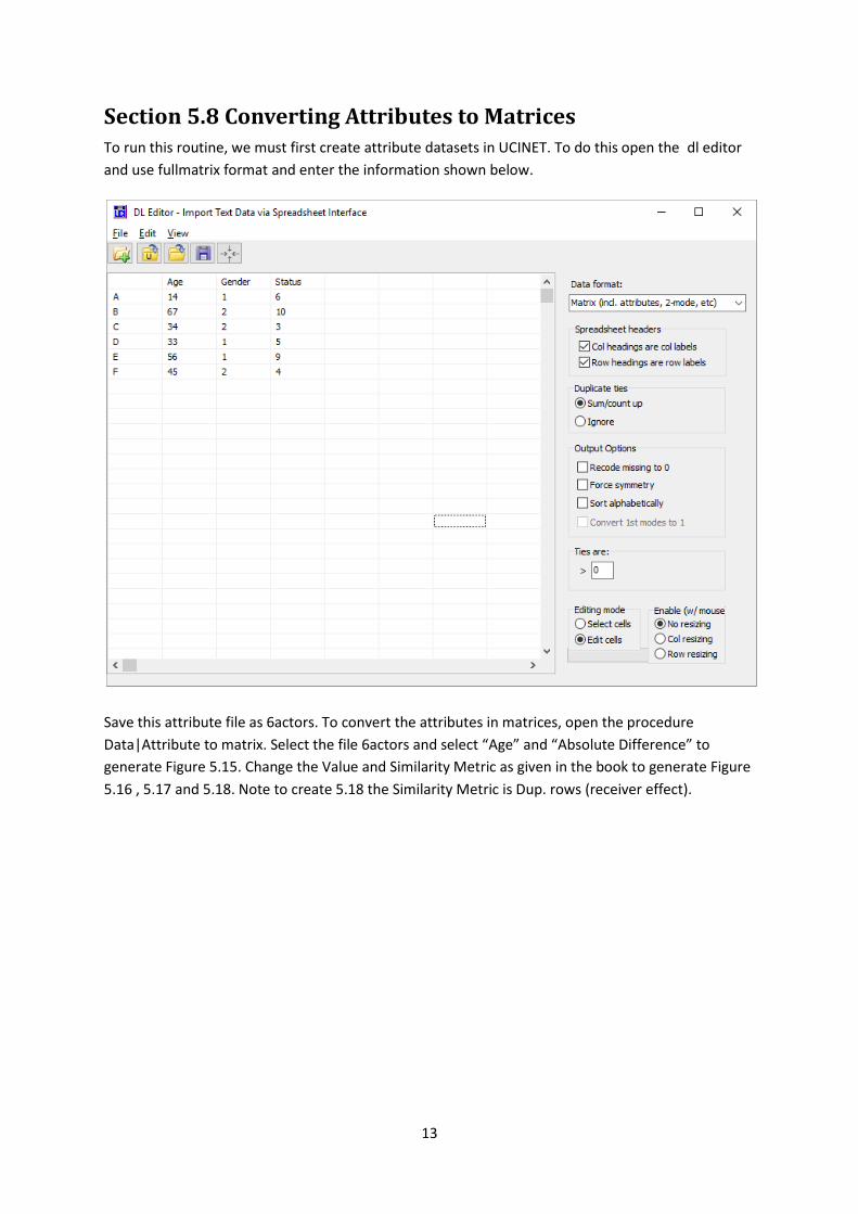
Section 5.8 Converting Attributes to Matrices To run this routine, we must first create attribute datasets in UCINET. To do this open the dl editor

and use fullmatrix format and enter the information shown below.

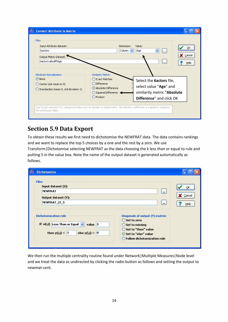
Save this attribute file as 6actors. To convert the attributes in matrices, open the procedure

Data|Attribute to matrix. Select the file 6actors and select “Age” and “Absolute Difference” to

generate Figure 5.15. Change the Value and Similarity Metric as given in the book to generate Figure

5.16 , 5.17 and 5.18. Note to create 5.18 the Similarity Metric is Dup. rows (receiver effect).

14

Section 5.9 Data Export To obtain these results we first need to dichotomise the NEWFRAT data. The data contains rankings

and we want to replace the top 5 choices by a one and the rest by a zero. We use

Transform|Dichotomise selecting NEWFRAT as the data choosing the k less than or equal to rule and

putting 5 in the value box. Note the name of the output dataset is generated automatically as

follows.

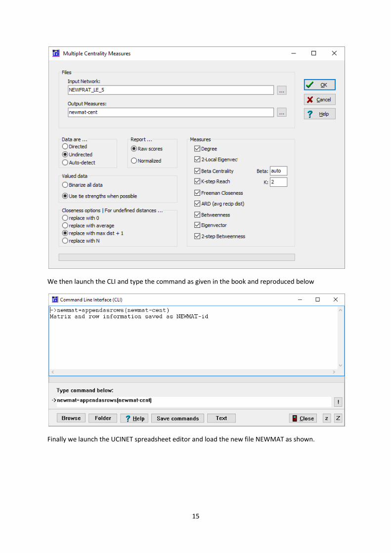
We then run the multiple centrality routine found under Network|Multiple Measures|Node level

and we treat the data as undirected by clicking the radio button as follows and setting the output to

newmat-cent.

Select the 6actors file,

select value “Age” and

similarity metric “Absolute

Difference” and click OK

15

We then launch the CLI and type the command as given in the book and reproduced below

Finally we launch the UCINET spreadsheet editor and load the new file NEWMAT as shown.

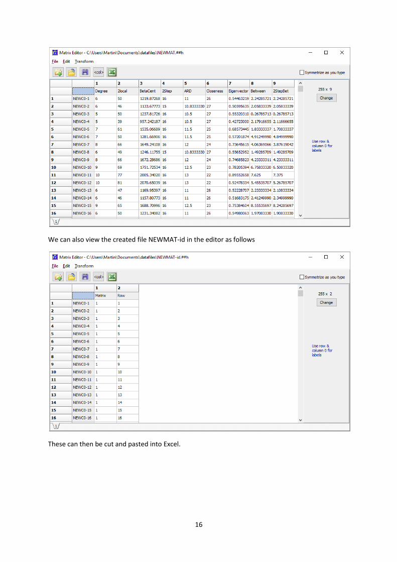
16

We can also view the created file NEWMAT-id in the editor as follows

These can then be cut and pasted into Excel.

17

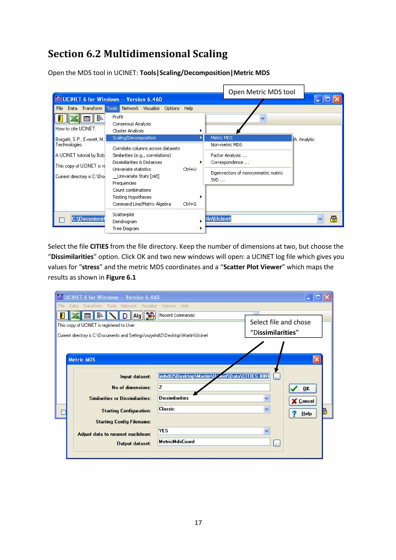
Section 6.2 Multidimensional Scaling

Open the MDS tool in UCINET: Tools|Scaling/Decomposition|Metric MDS

Select the file CITIES from the file directory. Keep the number of dimensions at two, but choose the

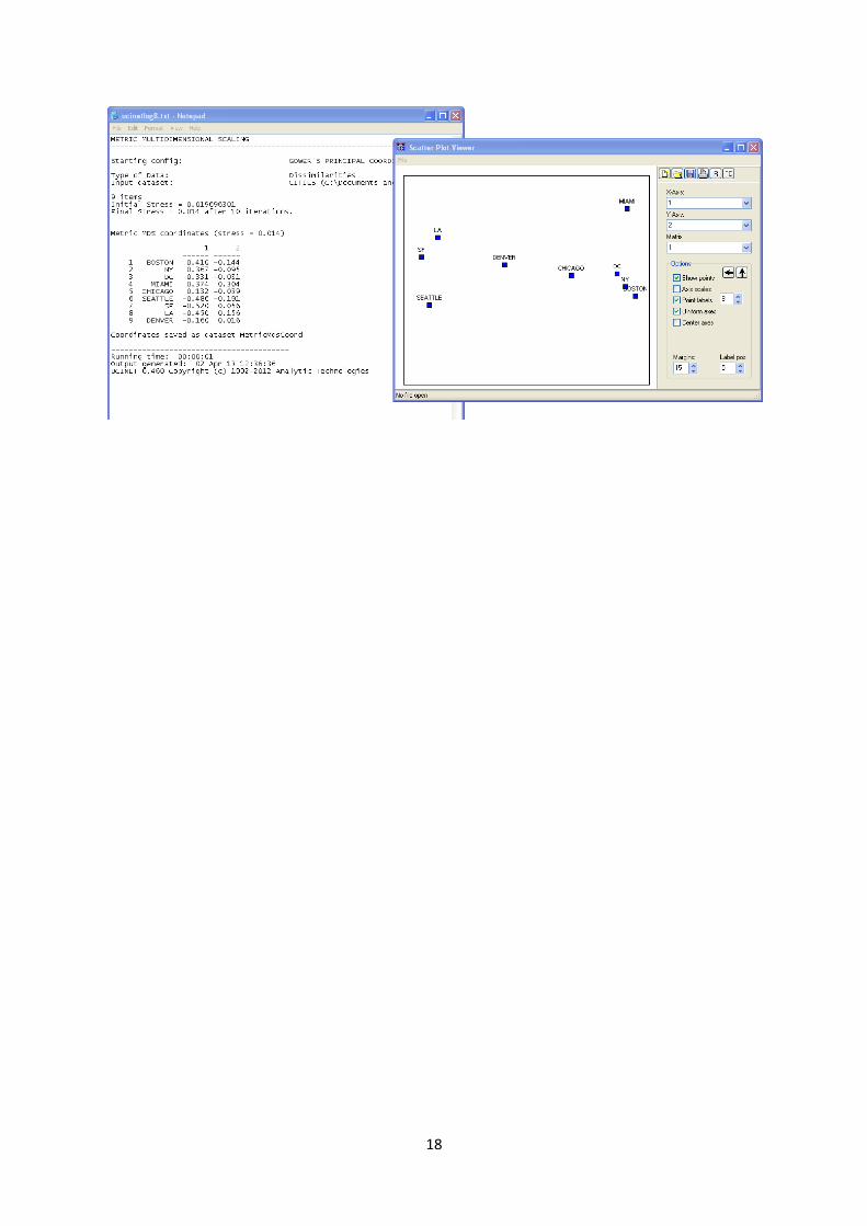
“Dissimilarities” option. Click OK and two new windows will open: a UCINET log file which gives you

values for “stress” and the metric MDS coordinates and a “Scatter Plot Viewer” which maps the

results as shown in Figure 6.1

Open Metric MDS tool

Select file and chose

“Dissimilarities”

18

19

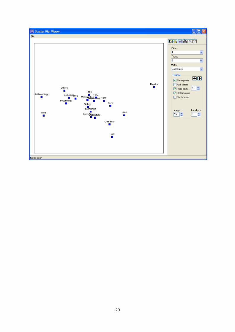
Section 6.3 Correspondence Analysis To reproduce Figure 6.2 run Tools|Scaling/Decomposition|Correspondence on the dataset leaving

all the defaults alone.

This produces the following as shown in the book.

20

21

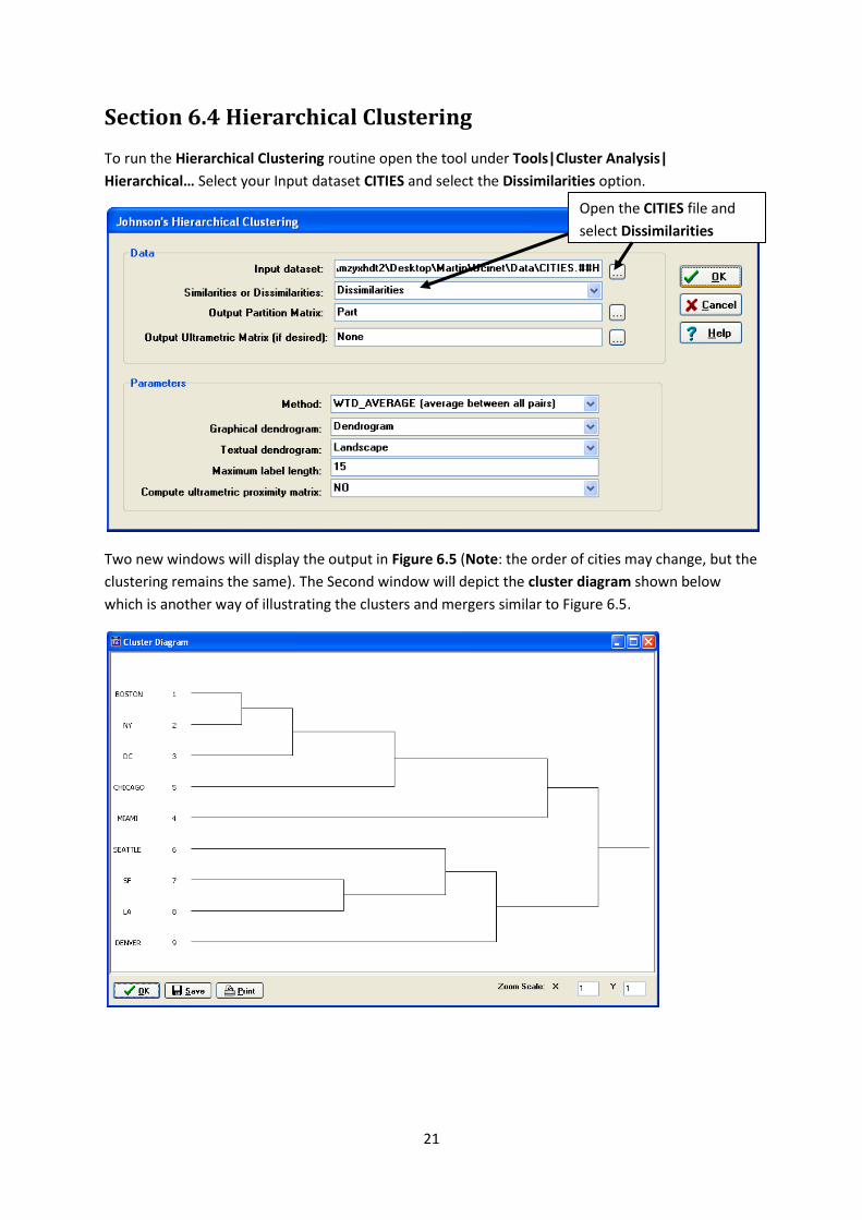
Section 6.4 Hierarchical Clustering

To run the Hierarchical Clustering routine open the tool under Tools|Cluster Analysis|

Hierarchical… Select your Input dataset CITIES and select the Dissimilarities option.

Two new windows will display the output in Figure 6.5 (Note: the order of cities may change, but the

clustering remains the same). The Second window will depict the cluster diagram shown below

which is another way of illustrating the clusters and mergers similar to Figure 6.5.

Open the CITIES file and

select Dissimilarities

22

Section 7.2 Layout

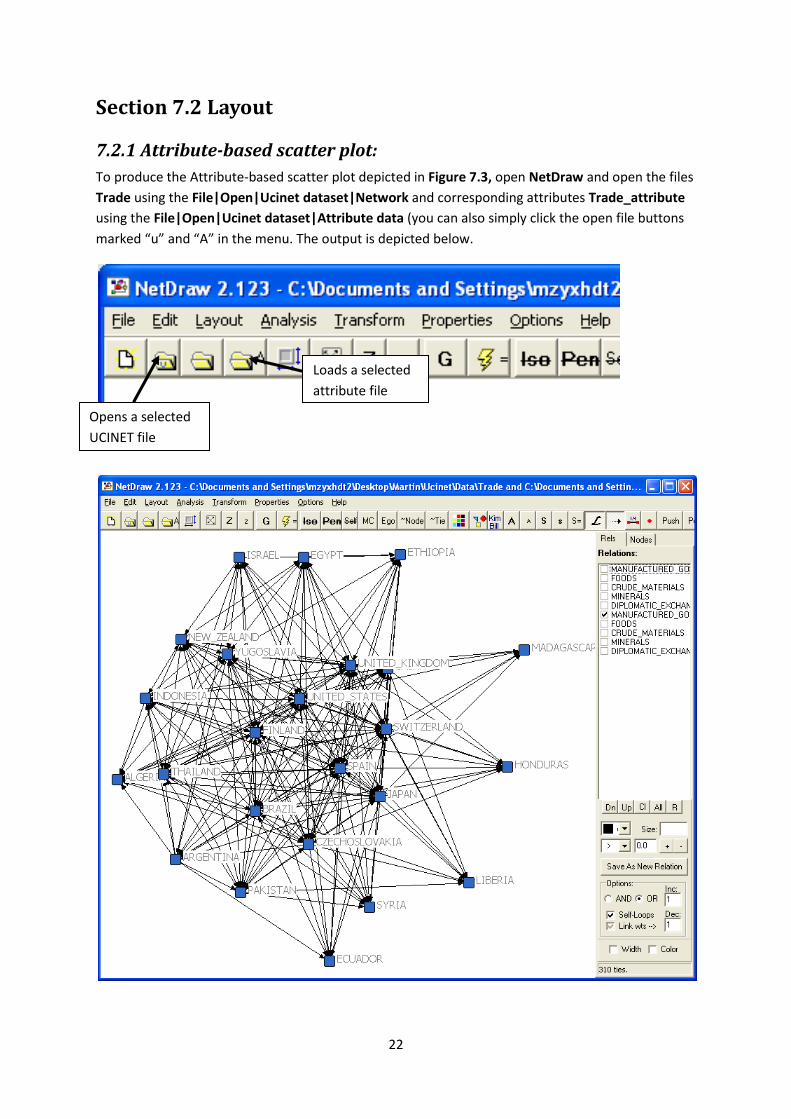
7.2.1 Attribute-based scatter plot:

To produce the Attribute-based scatter plot depicted in Figure 7.3, open NetDraw and open the files

Trade using the File|Open|Ucinet dataset|Network and corresponding attributes Trade_attribute

using the File|Open|Ucinet dataset|Attribute data (you can also simply click the open file buttons

marked “u” and “A” in the menu. The output is depicted below.

Opens a selected

UCINET file

Loads a selected

attribute file

23

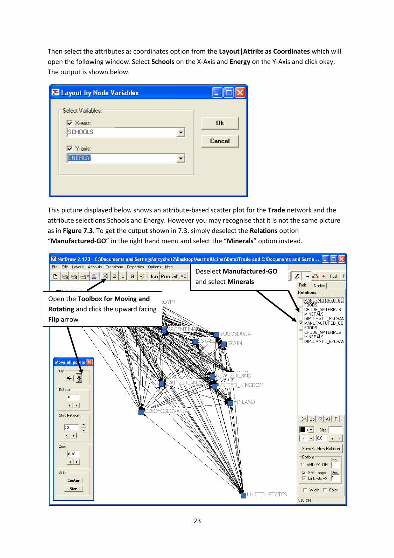
Then select the attributes as coordinates option from the Layout|Attribs as Coordinates which will

open the following window. Select Schools on the X-Axis and Energy on the Y-Axis and click okay.

The output is shown below.

This picture displayed below shows an attribute-based scatter plot for the Trade network and the

attribute selections Schools and Energy. However you may recognise that it is not the same picture

as in Figure 7.3. To get the output shown in 7.3, simply deselect the Relations option

“Manufactured-GO” in the right hand menu and select the “Minerals” option instead.

Deselect Manufactured-GO

and select Minerals

Open the Toolbox for Moving and

Rotating and click the upward facing

Flip arrow

24

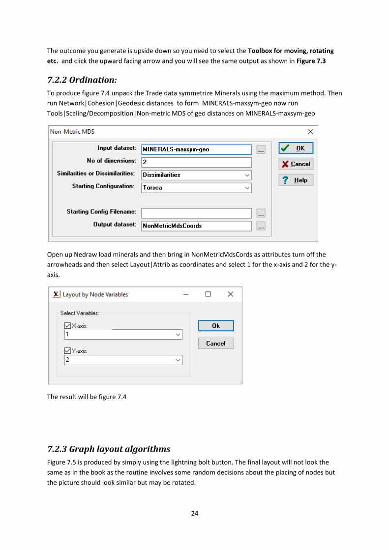
The outcome you generate is upside down so you need to select the Toolbox for moving, rotating

etc. and click the upward facing arrow and you will see the same output as shown in Figure 7.3

7.2.2 Ordination:

To produce figure 7.4 unpack the Trade data symmetrize Minerals using the maximum method. Then

run Network|Cohesion|Geodesic distances to form MINERALS-maxsym-geo now run

Tools|Scaling/Decomposition|Non-metric MDS of geo distances on MINERALS-maxsym-geo

Open up Nedraw load minerals and then bring in NonMetricMdsCords as attributes turn off the

arrowheads and then select Layout|Attrib as coordinates and select 1 for the x-axis and 2 for the y-

axis.

The result will be figure 7.4

7.2.3 Graph layout algorithms

Figure 7.5 is produced by simply using the lightning bolt button. The final layout will not look the

same as in the book as the routine involves some random decisions about the placing of nodes but

the picture should look similar but may be rotated.

25

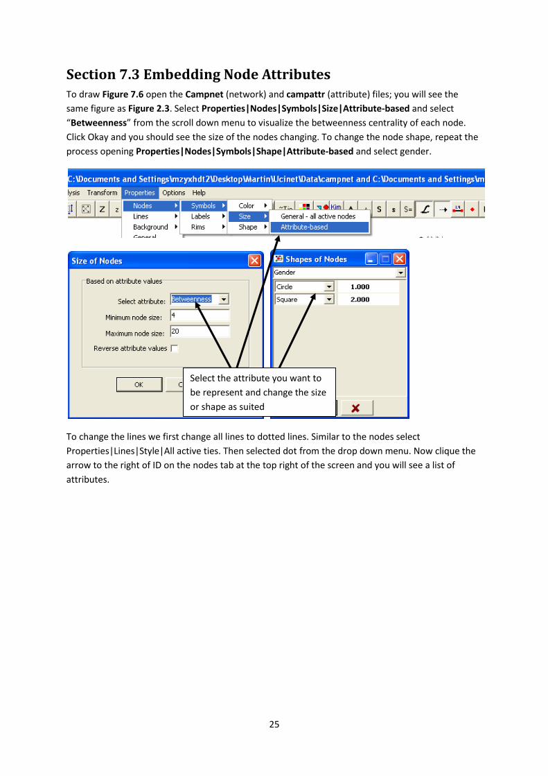
Section 7.3 Embedding Node Attributes To draw Figure 7.6 open the Campnet (network) and campattr (attribute) files; you will see the

same figure as Figure 2.3. Select Properties|Nodes|Symbols|Size|Attribute-based and select

“Betweenness” from the scroll down menu to visualize the betweenness centrality of each node.

Click Okay and you should see the size of the nodes changing. To change the node shape, repeat the

process opening Properties|Nodes|Symbols|Shape|Attribute-based and select gender.

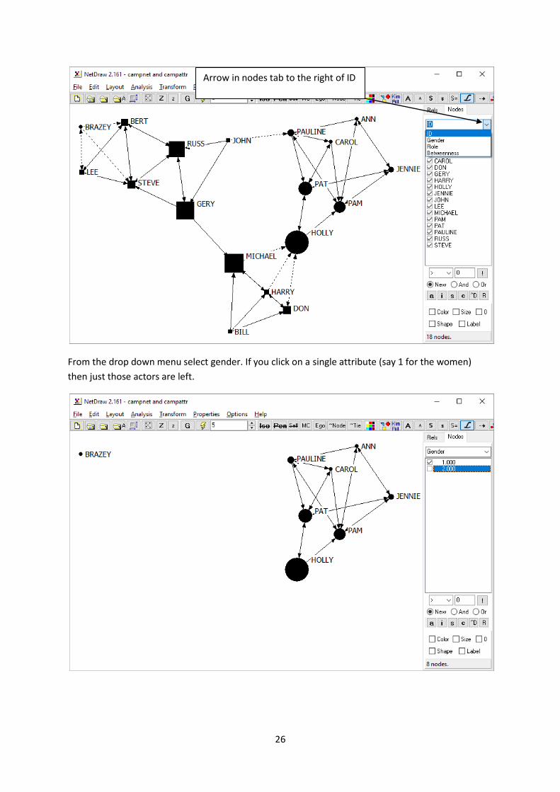
To change the lines we first change all lines to dotted lines. Similar to the nodes select

Properties|Lines|Style|All active ties. Then selected dot from the drop down menu. Now clique the

arrow to the right of ID on the nodes tab at the top right of the screen and you will see a list of

attributes.

Select the attribute you want to

be represent and change the size

or shape as suited

26

From the drop down menu select gender. If you click on a single attribute (say 1 for the women)

then just those actors are left.

Arrow in nodes tab to the right of ID

27

Now change the active edges to solid lines the same way as the dotted ones were created. Do the

same for the other attribute. Highlighting all attributes will result in Figure 7.6. This is also illustrated

in the next section.

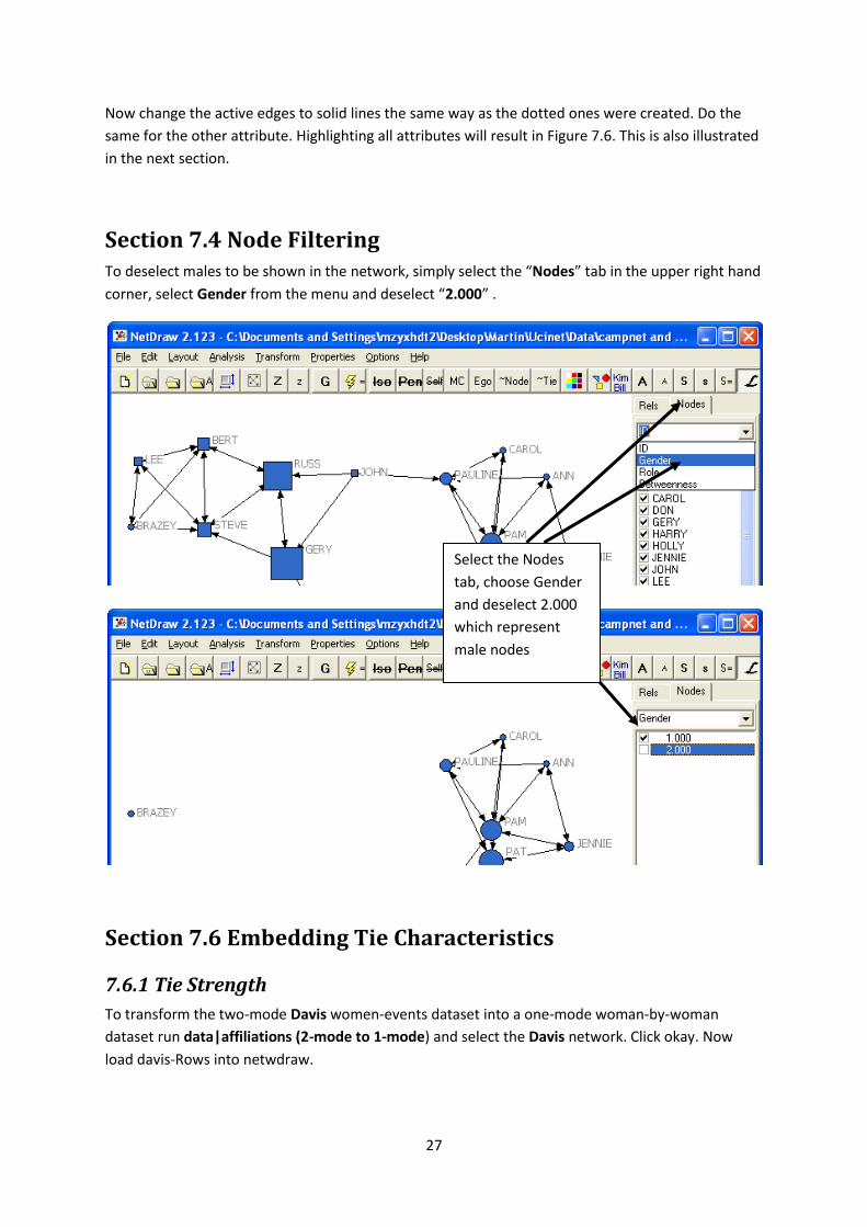
Section 7.4 Node Filtering To deselect males to be shown in the network, simply select the “Nodes” tab in the upper right hand

corner, select Gender from the menu and deselect “2.000” .

Section 7.6 Embedding Tie Characteristics

7.6.1 Tie Strength

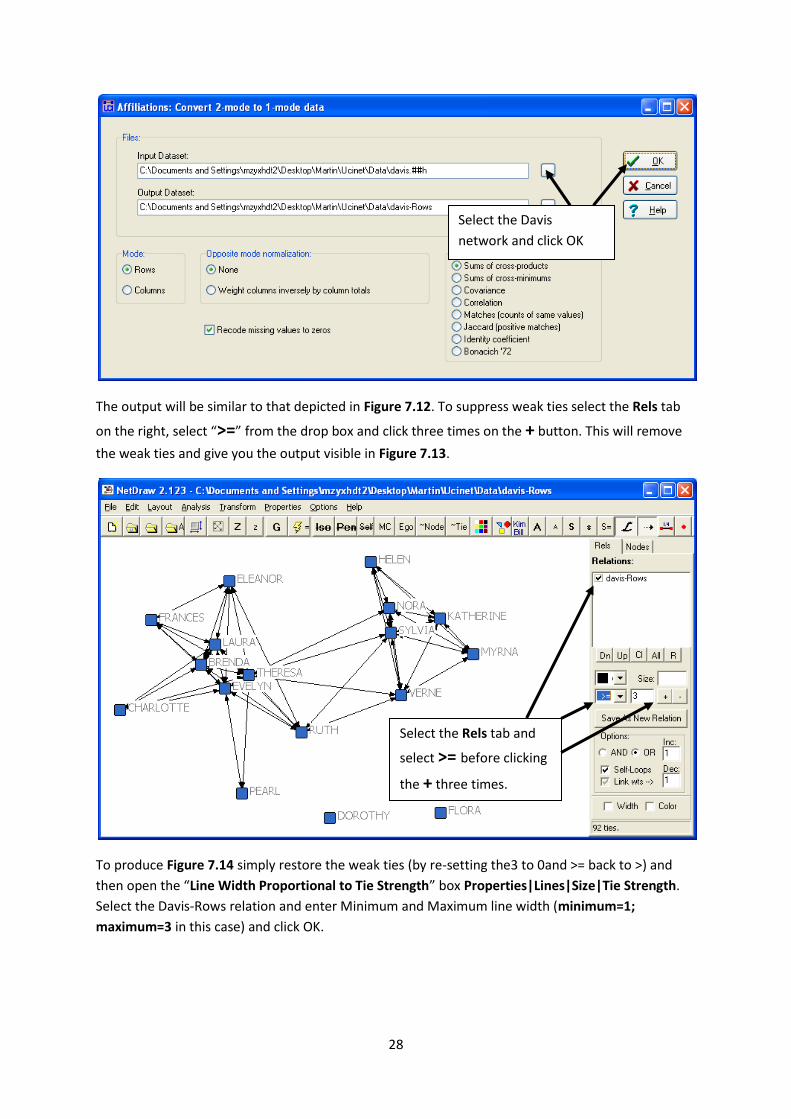
To transform the two-mode Davis women-events dataset into a one-mode woman-by-woman

dataset run data|affiliations (2-mode to 1-mode) and select the Davis network. Click okay. Now

load davis-Rows into netwdraw.

Select the Nodes

tab, choose Gender

and deselect 2.000

which represent

male nodes

28

The output will be similar to that depicted in Figure 7.12. To suppress weak ties select the Rels tab

on the right, select “>=” from the drop box and click three times on the + button. This will remove

the weak ties and give you the output visible in Figure 7.13.

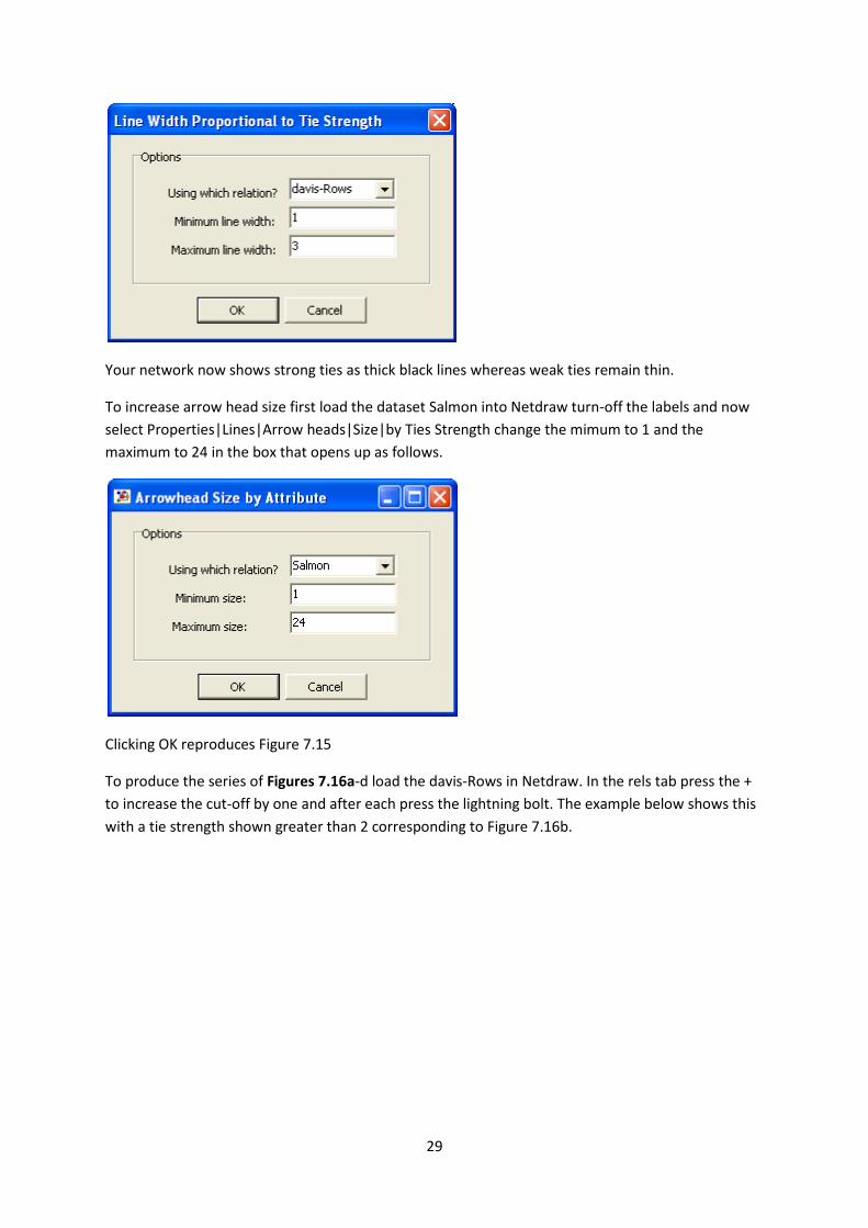
To produce Figure 7.14 simply restore the weak ties (by re-setting the3 to 0and >= back to >) and

then open the “Line Width Proportional to Tie Strength” box Properties|Lines|Size|Tie Strength.

Select the Davis-Rows relation and enter Minimum and Maximum line width (minimum=1;

maximum=3 in this case) and click OK.

Select the Davis

network and click OK

Select the Rels tab and

select >= before clicking

the + three times.

29

Your network now shows strong ties as thick black lines whereas weak ties remain thin.

To increase arrow head size first load the dataset Salmon into Netdraw turn-off the labels and now

select Properties|Lines|Arrow heads|Size|by Ties Strength change the mimum to 1 and the

maximum to 24 in the box that opens up as follows.

Clicking OK reproduces Figure 7.15

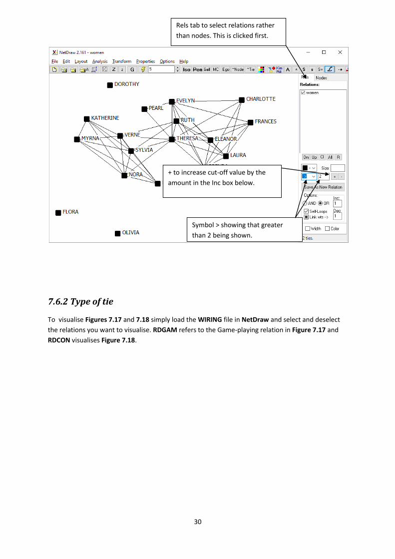
To produce the series of Figures 7.16a-d load the davis-Rows in Netdraw. In the rels tab press the +

to increase the cut-off by one and after each press the lightning bolt. The example below shows this

with a tie strength shown greater than 2 corresponding to Figure 7.16b.

30

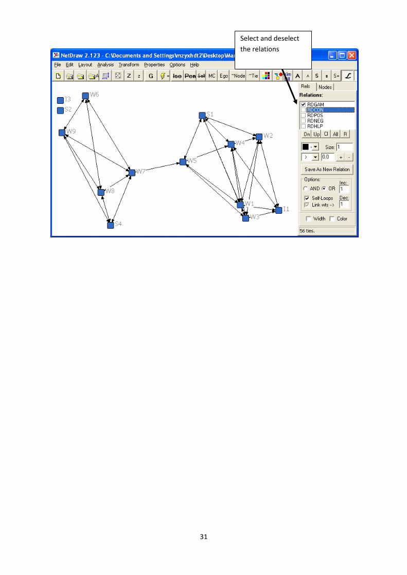
7.6.2 Type of tie

To visualise Figures 7.17 and 7.18 simply load the WIRING file in NetDraw and select and deselect

the relations you want to visualise. RDGAM refers to the Game-playing relation in Figure 7.17 and

RDCON visualises Figure 7.18.

Rels tab to select relations rather

than nodes. This is clicked first.

+ to increase cut-off value by the

amount in the Inc box below.

Symbol > showing that greater

than 2 being shown.

31

Select and deselect

the relations

32

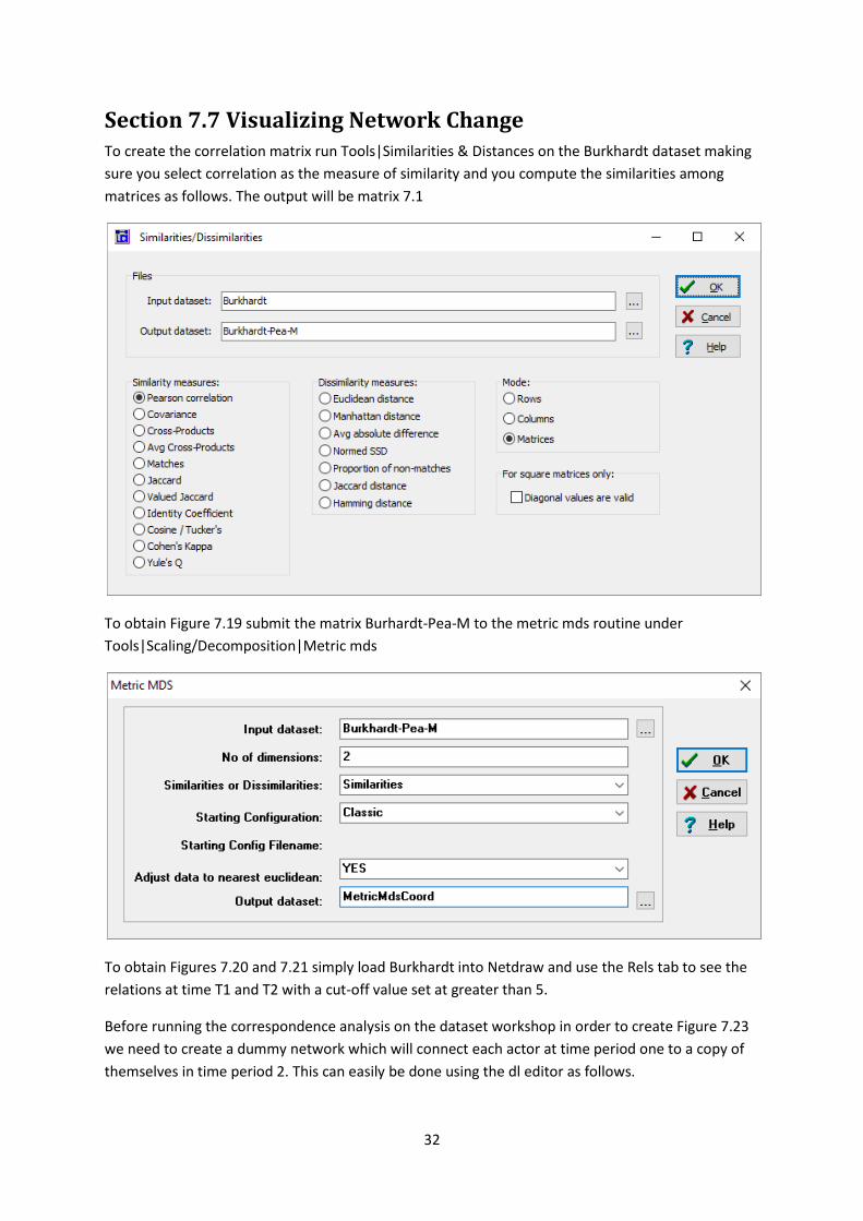
Section 7.7 Visualizing Network Change To create the correlation matrix run Tools|Similarities & Distances on the Burkhardt dataset making

sure you select correlation as the measure of similarity and you compute the similarities among

matrices as follows. The output will be matrix 7.1

To obtain Figure 7.19 submit the matrix Burhardt-Pea-M to the metric mds routine under

Tools|Scaling/Decomposition|Metric mds

To obtain Figures 7.20 and 7.21 simply load Burkhardt into Netdraw and use the Rels tab to see the

relations at time T1 and T2 with a cut-off value set at greater than 5.

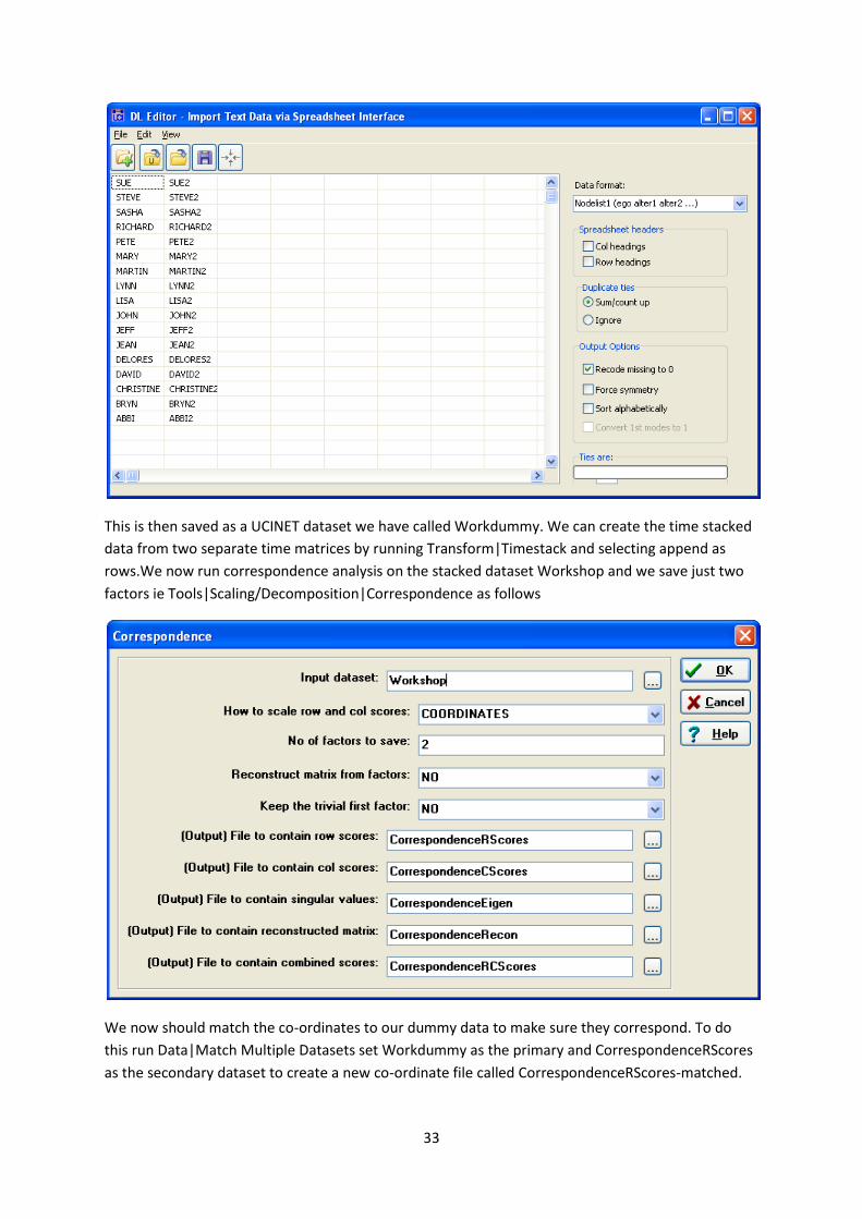
Before running the correspondence analysis on the dataset workshop in order to create Figure 7.23

we need to create a dummy network which will connect each actor at time period one to a copy of

themselves in time period 2. This can easily be done using the dl editor as follows.

33

This is then saved as a UCINET dataset we have called Workdummy. We can create the time stacked

data from two separate time matrices by running Transform|Timestack and selecting append as

rows.We now run correspondence analysis on the stacked dataset Workshop and we save just two

factors ie Tools|Scaling/Decomposition|Correspondence as follows

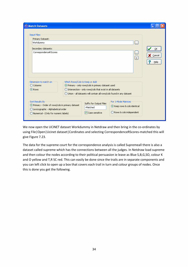
We now should match the co-ordinates to our dummy data to make sure they correspond. To do

this run Data|Match Multiple Datasets set Workdummy as the primary and CorrespondenceRScores

as the secondary dataset to create a new co-ordinate file called CorrespondenceRScores-matched.

34

We now open the UCINET dataset Workdummy in Netdraw and then bring in the co-ordinates by

using File|Open|Ucinet dataset|Cordinates and selecting CorrespondenceRScores-matched this will

give Figure 7.23.

The data for the supreme court for the correspondence analysis is called Supremeall there is also a

dataset called supreme which has the connections between all the judges. In Netdraw load supreme

and then colour the nodes according to their political persuasion ie leave as Blue S,B,G,SO, colour K

and O yellow and T,R SC red. This can easily be done since the trails are in separate components and

you can left click to open up a box that covers each trail in turn and colour groups of nodes. Once

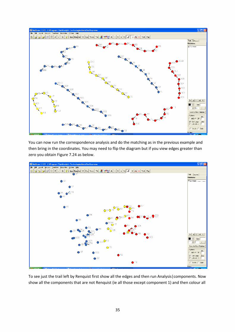
this is done you get the following.

35

You can now run the correspondence analysis and do the matching as in the previous example and

then bring in the coordinates. You may need to flip the diagram but if you view edges greater than

zero you obtain Figure 7.24 as below.

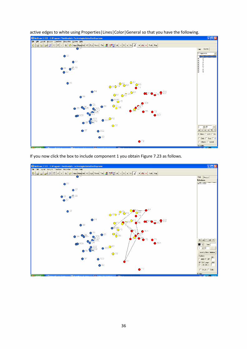
To see just the trail left by Renquist first show all the edges and then run Analysis|components. Now

show all the components that are not Renquist (ie all those except component 1) and then colour all

36

active edges to white using Properties|Lines|Color|General so that you have the following.

If you now click the box to include component 1 you obtain Figure 7.23 as follows.

37

Section 8.3 Dyadic Hypothesis

QAP Correlation

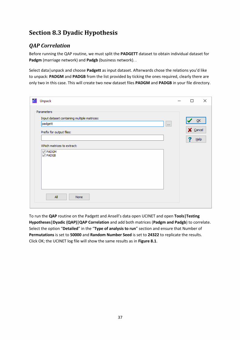
Before running the QAP routine, we must split the PADGETT dataset to obtain individual dataset for

Padgm (marriage network) and Padgb (business network). .

Select data|unpack and choose Padgett as input dataset. Afterwards chose the relations you’d like

to unpack: PADGM and PADGB from the list provided by ticking the ones required, clearly there are

only two in this case. This will create two new dataset files PADGM and PADGB in your file directory.

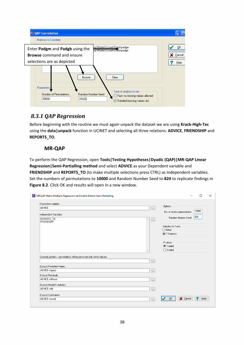
To run the QAP routine on the Padgett and Ansell’s data open UCINET and open Tools|Testing

Hypotheses|Dyadic (QAP)|QAP Correlation and add both matrices (Padgm and Padgb) to correlate.

Select the option “Detailed” in the “Type of analysis to run” section and ensure that Number of

Permutations is set to 50000 and Random Number Seed is set to 24322 to replicate the results.

Click OK; the UCINET log file will show the same results as in Figure 8.1.

38

8.3.1 QAP Regression

Before beginning with the routine we must again unpack the dataset we are using Krack-High-Tec

using the data|unpack function in UCINET and selecting all three relations: ADVICE, FRIENDSHIP and

REPORTS_TO.

MR-QAP

To perform the QAP Regression, open Tools|Testing Hypotheses|Dyadic (QAP)|MR-QAP Linear

Regression|Semi-Partialling method and select ADVICE as your Dependent variable and

FRIENDSHIP and REPORTS_TO (to make multiple selections press CTRL) as Independent variables.

Set the numbers of permutations to 10000 and Random Number Seed to 824 to replicate findings in

Figure 8.2. Click OK and results will open in a new window.

Enter Padgm and Padgb using the

Browse command and ensure

selections are as depicted

39

LR-QAP

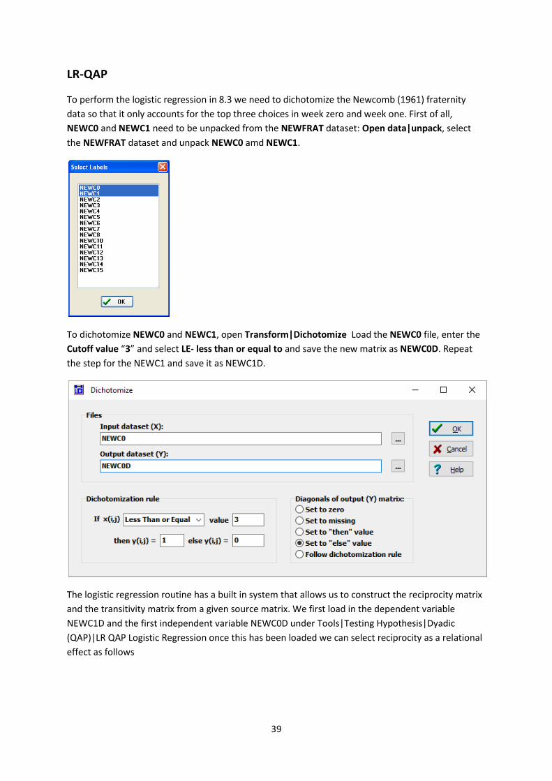
To perform the logistic regression in 8.3 we need to dichotomize the Newcomb (1961) fraternity

data so that it only accounts for the top three choices in week zero and week one. First of all,

NEWC0 and NEWC1 need to be unpacked from the NEWFRAT dataset: Open data|unpack, select

the NEWFRAT dataset and unpack NEWC0 amd NEWC1.

To dichotomize NEWC0 and NEWC1, open Transform|Dichotomize Load the NEWC0 file, enter the

Cutoff value “3” and select LE- less than or equal to and save the new matrix as NEWC0D. Repeat

the step for the NEWC1 and save it as NEWC1D.

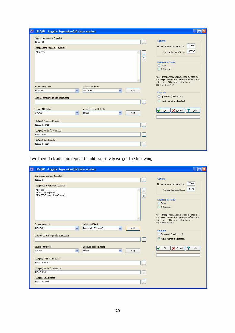
The logistic regression routine has a built in system that allows us to construct the reciprocity matrix

and the transitivity matrix from a given source matrix. We first load in the dependent variable

NEWC1D and the first independent variable NEWC0D under Tools|Testing Hypothesis|Dyadic

(QAP)|LR QAP Logistic Regression once this has been loaded we can select reciprocity as a relational

effect as follows

40

If we then click add and repeat to add transitivity we get the following

41

If we now press OK we get similar results to the ones in the book. The number of permutations are

not quite high enough to obtain an exact replication but the significance levels should be very close.

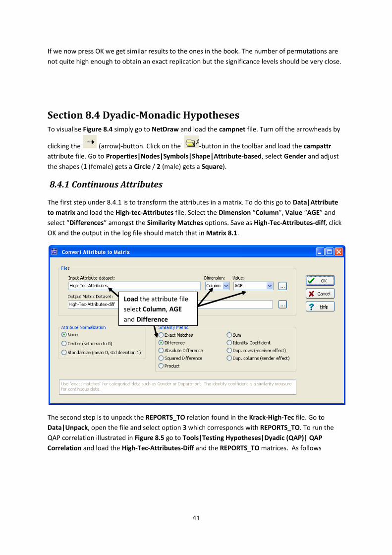
Section 8.4 Dyadic-Monadic Hypotheses To visualise Figure 8.4 simply go to NetDraw and load the campnet file. Turn off the arrowheads by

clicking the (arrow)-button. Click on the -button in the toolbar and load the campattr

attribute file. Go to Properties|Nodes|Symbols|Shape|Attribute-based, select Gender and adjust

the shapes (1 (female) gets a Circle / 2 (male) gets a Square).

8.4.1 Continuous Attributes

The first step under 8.4.1 is to transform the attributes in a matrix. To do this go to Data|Attribute

to matrix and load the High-tec-Attributes file. Select the Dimension “Column”, Value “AGE” and

select “Differences” amongst the Similarity Matches options. Save as High-Tec-Attributes-diff, click

OK and the output in the log file should match that in Matrix 8.1.

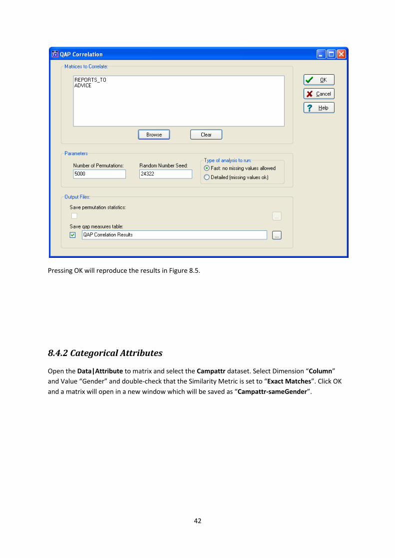
The second step is to unpack the REPORTS_TO relation found in the Krack-High-Tec file. Go to

Data|Unpack, open the file and select option 3 which corresponds with REPORTS_TO. To run the

QAP correlation illustrated in Figure 8.5 go to Tools|Testing Hypotheses|Dyadic (QAP)| QAP

Correlation and load the High-Tec-Attributes-Diff and the REPORTS_TO matrices. As follows

Load the attribute file

select Column, AGE

and Difference

42

Pressing OK will reproduce the results in Figure 8.5.

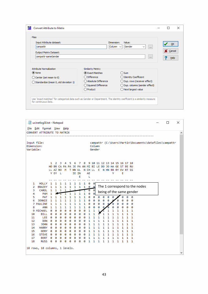
8.4.2 Categorical Attributes

Open the Data|Attribute to matrix and select the Campattr dataset. Select Dimension “Column”

and Value “Gender” and double-check that the Similarity Metric is set to “Exact Matches”. Click OK

and a matrix will open in a new window which will be saved as “Campattr-sameGender”.

43

The 1 correspond to the nodes

being of the same gender

44

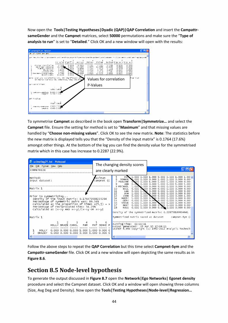
Now open the Tools|Testing Hypotheses|Dyadic (QAP)|QAP Correlation and insert the Campattr-

sameGender and the Campnet matrices, select 50000 permutations and make sure the “Type of

analysis to run” is set to “Detailed.” Click OK and a new window will open with the results:

To symmetrise Campnet as described in the book open Transform|Symmetrize… and select the

Campnet file. Ensure the setting for method is set to “Maximum” and that missing values are

handled by “Choose non-missing values”. Click OK to see the new matrix. Note: The statistics before

the new matrix is displayed tells you that the “Density of the input matrix” is 0.1764 (17.6%)

amongst other things. At the bottom of the log you can find the density value for the symmetrised

matrix which in this case has increase to 0.2287 (22.9%).

Follow the above steps to repeat the QAP Correlation but this time select Campnet-Sym and the

Campattr-sameGender file. Click OK and a new window will open depicting the same results as in

Figure 8.6.

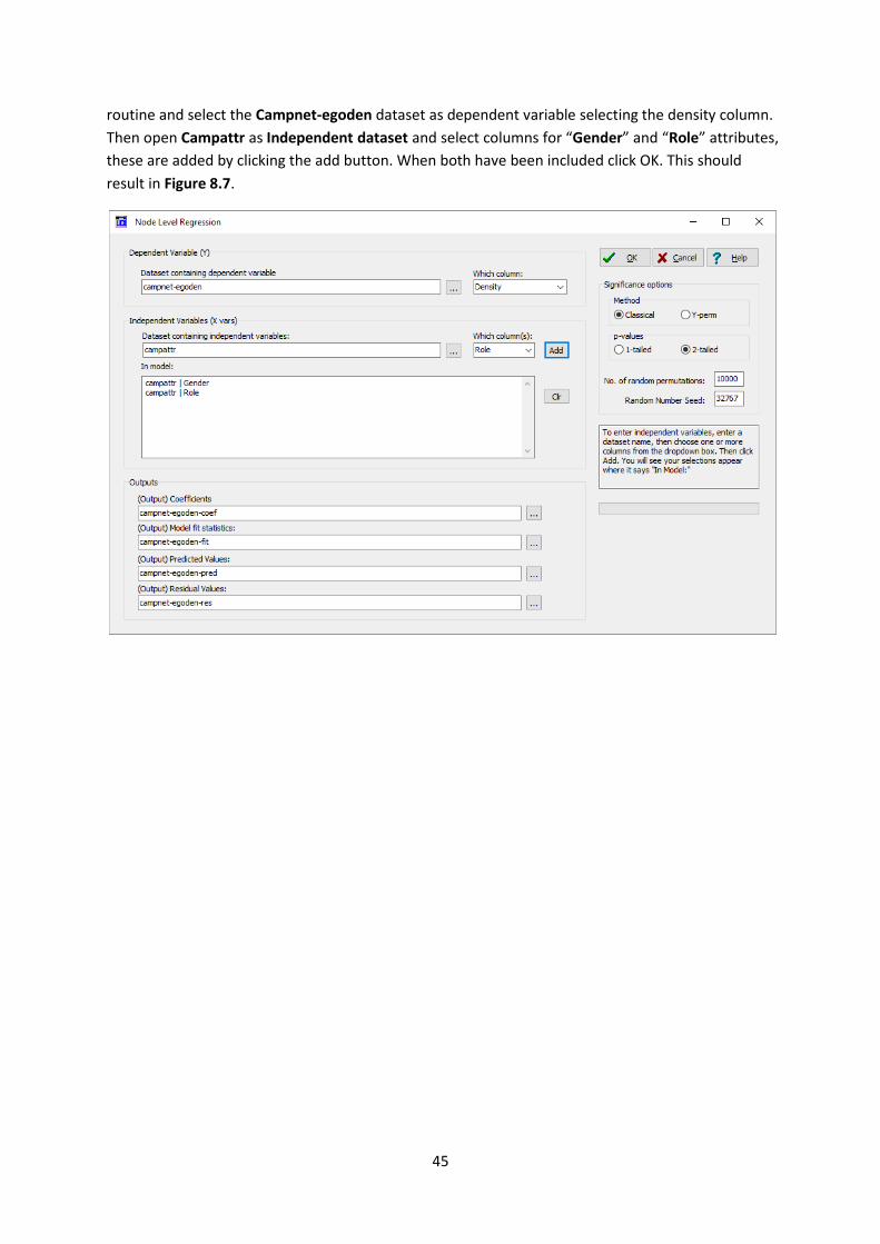
Section 8.5 Node-level hypothesis To generate the output discussed in Figure 8.7 open the Network|Ego Networks| Egonet density

procedure and select the Campnet dataset. Click OK and a window will open showing three columns

(Size, Avg Deg and Density). Now open the Tools|Testing Hypotheses|Node-level|Regression…

The changing density scores

are clearly marked

Values for correlation

P-Values

45

routine and select the Campnet-egoden dataset as dependent variable selecting the density column.

Then open Campattr as Independent dataset and select columns for “Gender” and “Role” attributes,

these are added by clicking the add button. When both have been included click OK. This should

result in Figure 8.7.

46

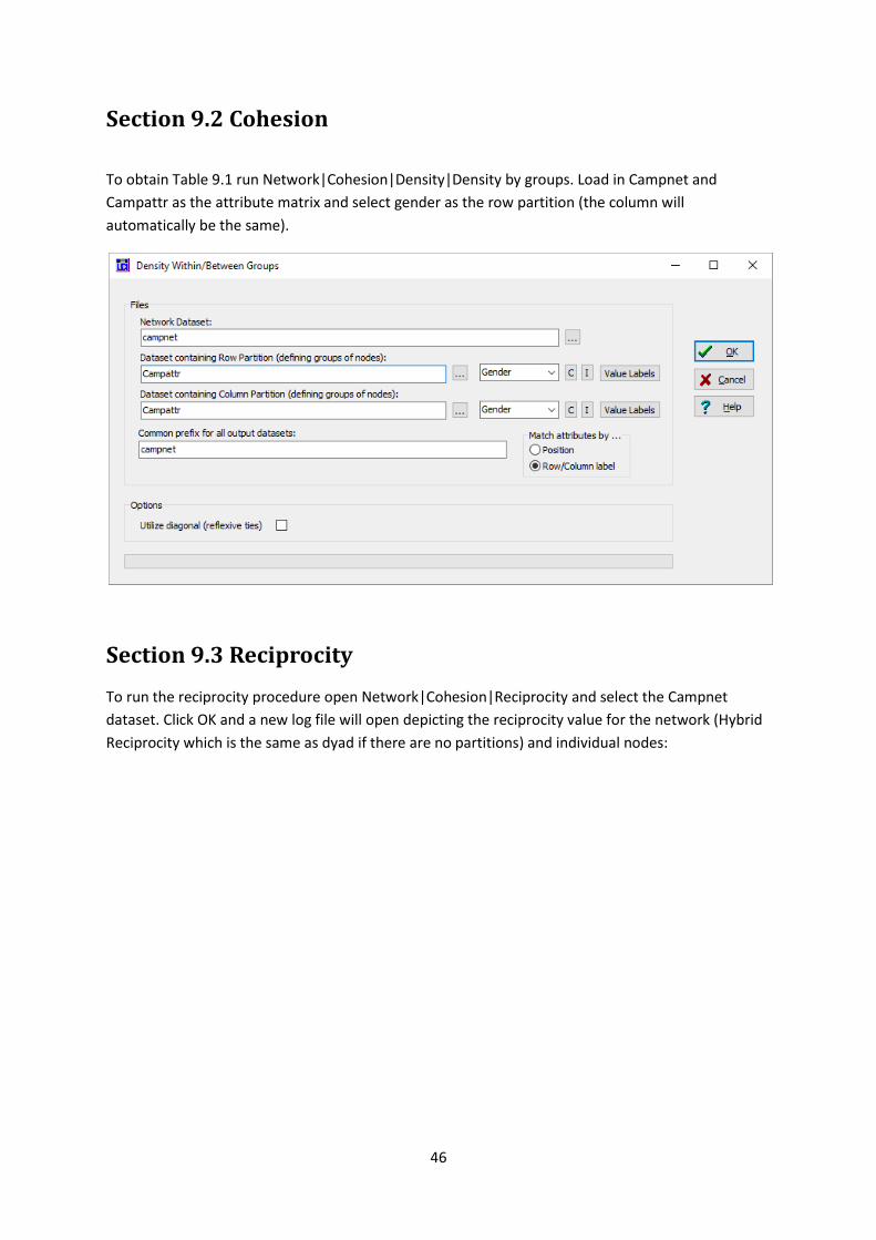
Section 9.2 Cohesion

To obtain Table 9.1 run Network|Cohesion|Density|Density by groups. Load in Campnet and

Campattr as the attribute matrix and select gender as the row partition (the column will

automatically be the same).

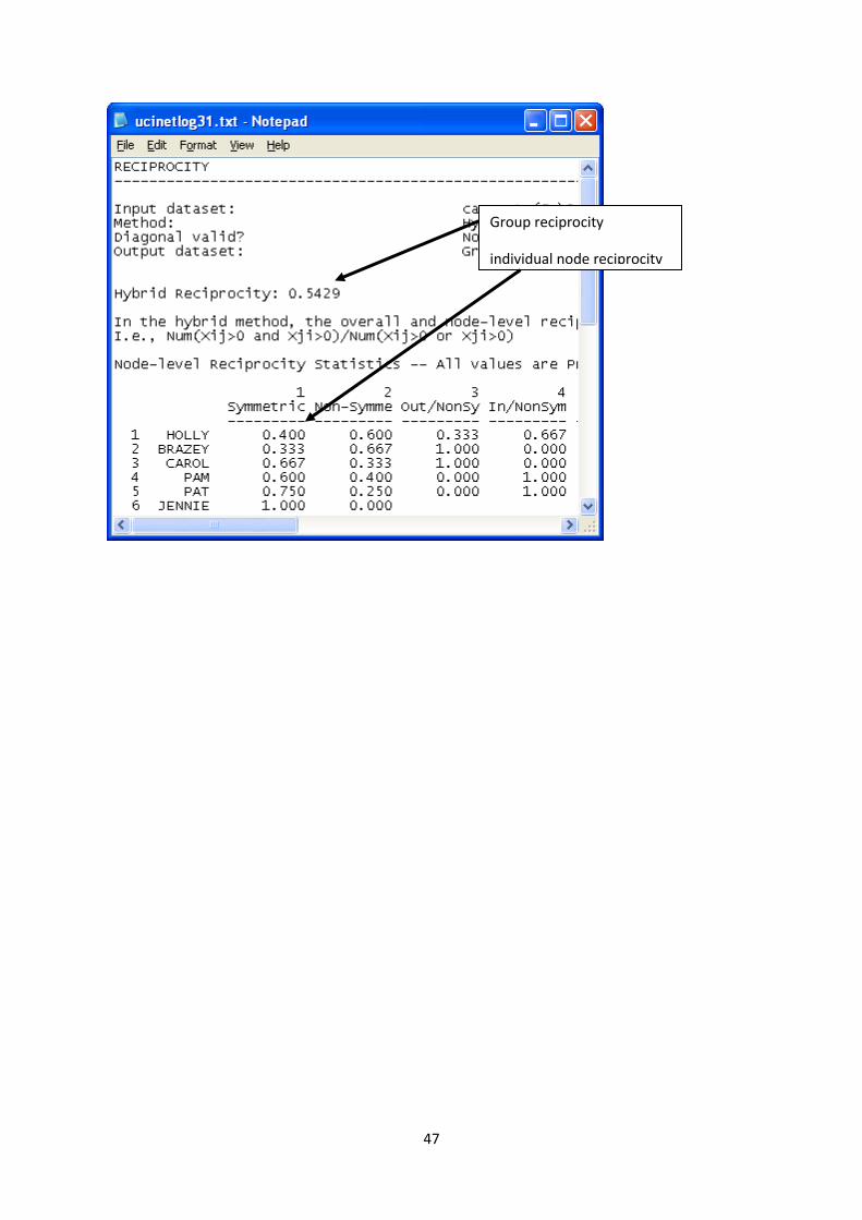
Section 9.3 Reciprocity

To run the reciprocity procedure open Network|Cohesion|Reciprocity and select the Campnet

dataset. Click OK and a new log file will open depicting the reciprocity value for the network (Hybrid

Reciprocity which is the same as dyad if there are no partitions) and individual nodes:

47

Group reciprocity

individual node reciprocity

48

Section 10.3 Undirected, Non-valued Networks

10.3.1 Degree Centrality

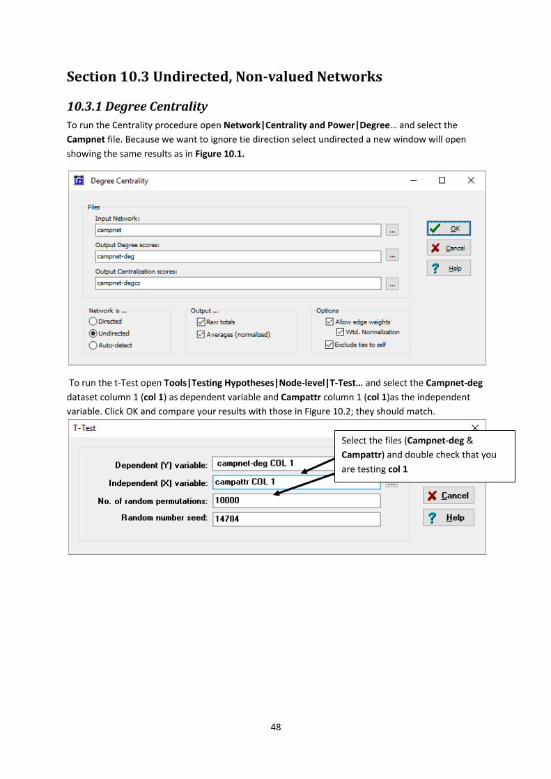
To run the Centrality procedure open Network|Centrality and Power|Degree… and select the

Campnet file. Because we want to ignore tie direction select undirected a new window will open

showing the same results as in Figure 10.1.

To run the t-Test open Tools|Testing Hypotheses|Node-level|T-Test… and select the Campnet-deg

dataset column 1 (col 1) as dependent variable and Campattr column 1 (col 1)as the independent

variable. Click OK and compare your results with those in Figure 10.2; they should match.

Select the files (Campnet-deg &

Campattr) and double check that you

are testing col 1

49

Section 11.2 Cliques

11.2.1 Analyzing clique overlaps

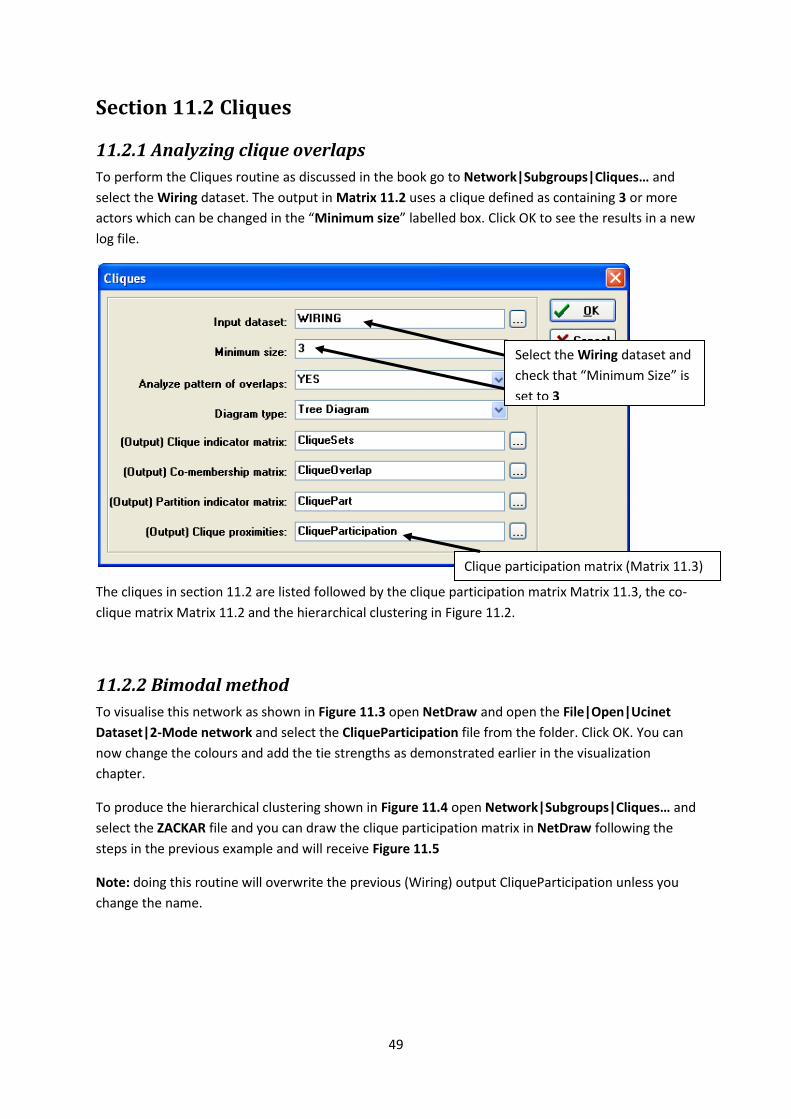
To perform the Cliques routine as discussed in the book go to Network|Subgroups|Cliques… and

select the Wiring dataset. The output in Matrix 11.2 uses a clique defined as containing 3 or more

actors which can be changed in the “Minimum size” labelled box. Click OK to see the results in a new

log file.

The cliques in section 11.2 are listed followed by the clique participation matrix Matrix 11.3, the co-

clique matrix Matrix 11.2 and the hierarchical clustering in Figure 11.2.

11.2.2 Bimodal method

To visualise this network as shown in Figure 11.3 open NetDraw and open the File|Open|Ucinet

Dataset|2-Mode network and select the CliqueParticipation file from the folder. Click OK. You can

now change the colours and add the tie strengths as demonstrated earlier in the visualization

chapter.

To produce the hierarchical clustering shown in Figure 11.4 open Network|Subgroups|Cliques… and

select the ZACKAR file and you can draw the clique participation matrix in NetDraw following the

steps in the previous example and will receive Figure 11.5

Note: doing this routine will overwrite the previous (Wiring) output CliqueParticipation unless you

change the name.

Select the Wiring dataset and

check that “Minimum Size” is

set to 3

Clique participation matrix (Matrix 11.3)

50

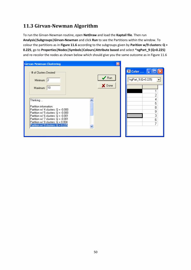
11.3 Girvan-Newman Algorithm

To run the Girvan-Newman routine, open NetDraw and load the Kaptail file. Then run

Analysis|Subgroups|Girvan-Newman and click Run to see the Partitions within the window. To

colour the partitions as in Figure 11.6 according to the subgroups given by Parition w/9 clusters: Q =

0.225, go to Properties|Nodes|Symbols|Colours|Attribute based and select *ngPart_9 (Q=0.225)

and re-recolor the nodes as shown below which should give you the same outcome as in Figure 11.6

51

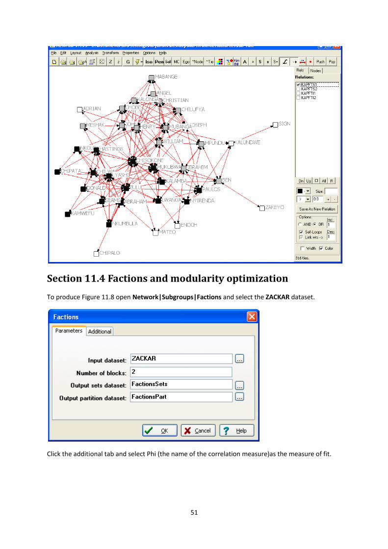
Section 11.4 Factions and modularity optimization

To produce Figure 11.8 open Network|Subgroups|Factions and select the ZACKAR dataset.

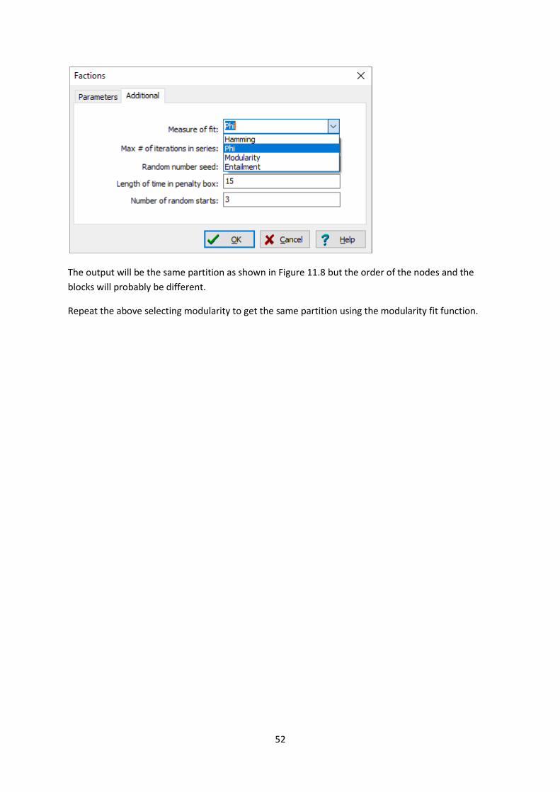
Click the additional tab and select Phi (the name of the correlation measure)as the measure of fit.

52

The output will be the same partition as shown in Figure 11.8 but the order of the nodes and the

blocks will probably be different.

Repeat the above selecting modularity to get the same partition using the modularity fit function.

53

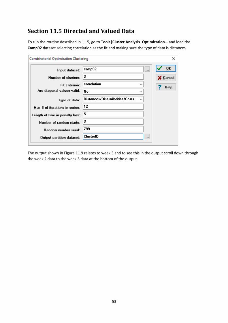
Section 11.5 Directed and Valued Data

To run the routine described in 11.5, go to Tools|Cluster Analysis|Optimization… and load the

Camp92 dataset selecting correlation as the fit and making sure the type of data is distances.

The output shown in Figure 11.9 relates to week 3 and to see this in the output scroll down through

the week 2 data to the week 3 data at the bottom of the output.

54

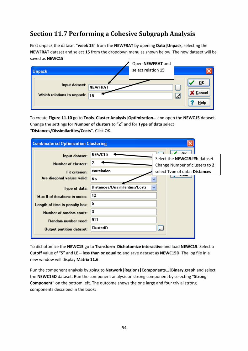
Section 11.7 Performing a Cohesive Subgraph Analysis

First unpack the dataset “week 15” from the NEWFRAT by opening Data|Unpack, selecting the

NEWFRAT dataset and select 15 from the dropdown menu as shown below. The new dataset will be

saved as NEWC15

To create Figure 11.10 go to Tools|Cluster Analysis|Optimization… and open the NEWC15 dataset.

Change the settings for Number of clusters to “2” and for Type of data select

“Distances/Dissimilarities/Costs”. Click OK.

To dichotomize the NEWC15 go to Transform|Dichotomize interactive and load NEWC15. Select a

Cutoff value of “5” and LE – less than or equal to and save dataset as NEWC15D. The log file in a

new window will display Matrix 11.6.

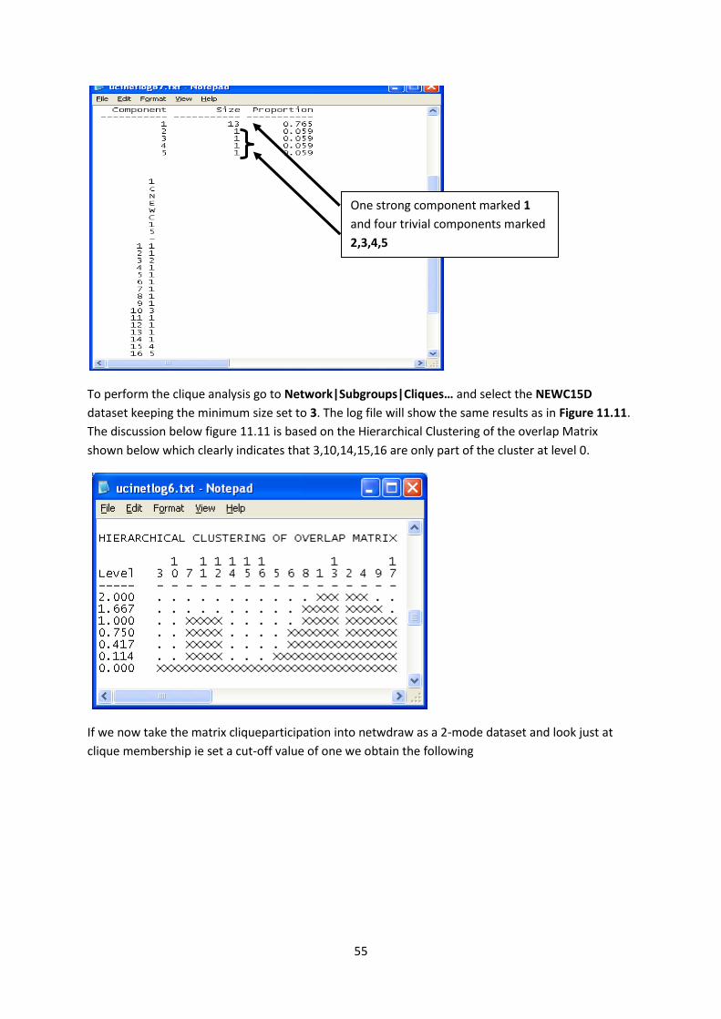
Run the component analysis by going to Network|Regions|Components…|Binary graph and select

the NEWC15D dataset. Run the component analysis on strong component by selecting “Strong

Component” on the bottom left. The outcome shows the one large and four trivial strong

components described in the book:

Select the NEWC15##h dataset

Change Number of clusters to 2

select Type of data: Distances

Open NEWFRAT and

select relation 15

55

To perform the clique analysis go to Network|Subgroups|Cliques… and select the NEWC15D

dataset keeping the minimum size set to 3. The log file will show the same results as in Figure 11.11.

The discussion below figure 11.11 is based on the Hierarchical Clustering of the overlap Matrix

shown below which clearly indicates that 3,10,14,15,16 are only part of the cluster at level 0.

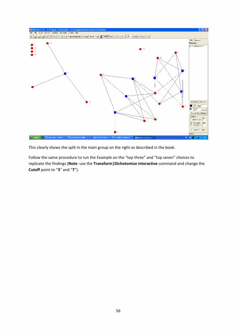
If we now take the matrix cliqueparticipation into netwdraw as a 2-mode dataset and look just at

clique membership ie set a cut-off value of one we obtain the following

One strong component marked 1

and four trivial components marked

2,3,4,5

56

This clearly shows the split in the main group on the right as described in the book.

Follow the same procedure to run the Example on the “top three” and “top seven” choices to

replicate the findings (Note: use the Transform|Dichotomize interactive command and change the

Cutoff point to “3” and “7”).

57

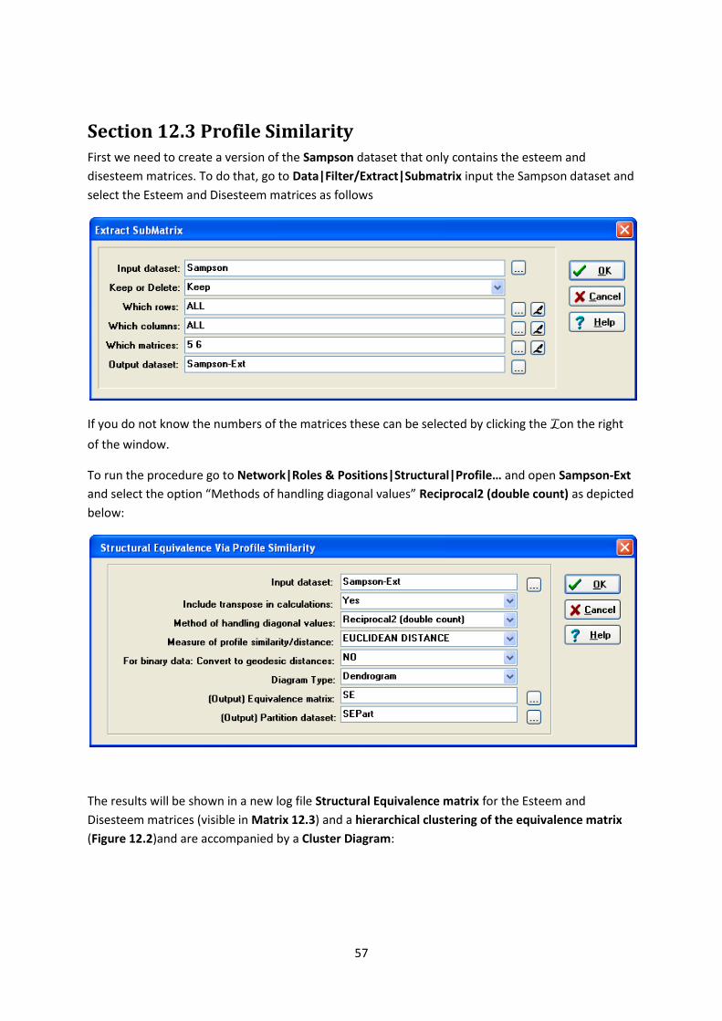
Section 12.3 Profile Similarity First we need to create a version of the Sampson dataset that only contains the esteem and

disesteem matrices. To do that, go to Data|Filter/Extract|Submatrix input the Sampson dataset and

select the Esteem and Disesteem matrices as follows

If you do not know the numbers of the matrices these can be selected by clicking the Lon the right

of the window.

To run the procedure go to Network|Roles & Positions|Structural|Profile… and open Sampson-Ext

and select the option “Methods of handling diagonal values” Reciprocal2 (double count) as depicted

below:

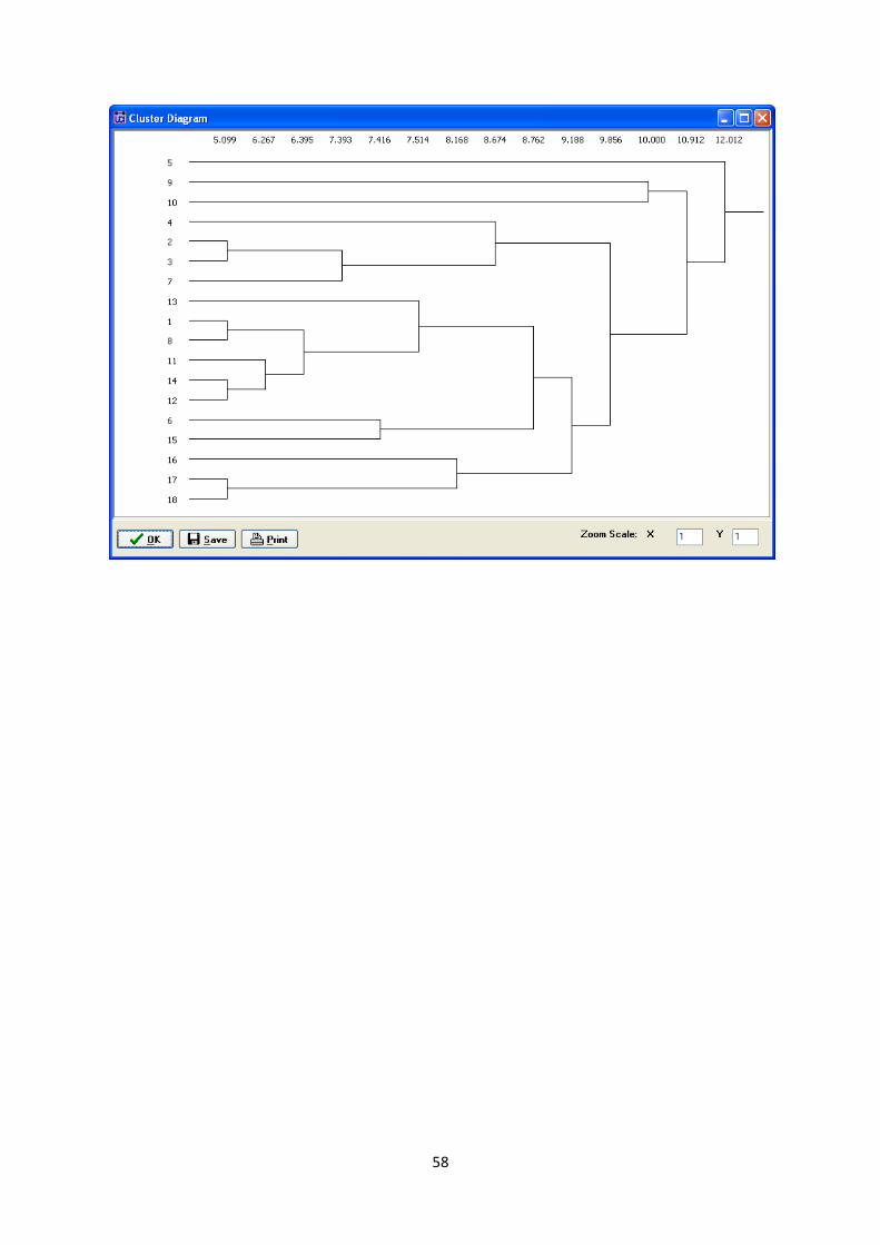
The results will be shown in a new log file Structural Equivalence matrix for the Esteem and

Disesteem matrices (visible in Matrix 12.3) and a hierarchical clustering of the equivalence matrix

(Figure 12.2)and are accompanied by a Cluster Diagram:

58

59

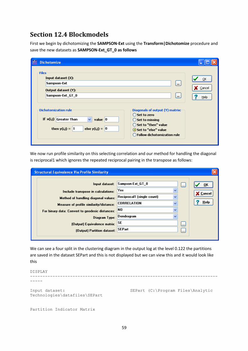
Section 12.4 Blockmodels First we begin by dichotomizing the SAMPSON-Ext using the Transform|Dichotomize procedure and

save the new datasets as SAMPSON-Ext_GT_0 as follows

We now run profile similarity on this selecting correlation and our method for handling the diagonal

is reciprocal1 which ignores the repeated reciprocal pairing in the transpose as follows:

We can see a four split in the clustering diagram in the output log at the level 0.122 the partitions

are saved in the dataset SEPart and this is not displayed but we can view this and it would look like

this

DISPLAY

---------------------------------------------------------------------------

-----

Input dataset: SEPart (C:\Program Files\Analytic

Technologies\datafiles\SEPart

Partition Indicator Matrix

60

1 2 3 4 5 6 7 8 9 10 11 12 13 14 15 16 17

0. 0. 0. 0. 0. 0. 0. 0. 0. 0. 0. 0. 0. 0. 0. -0 -0

83 64 61 46 43 41 37 36 35 30 24 23 13 12 10 .0 .0

2 0 6 8 9 0 7 0 8 5 1 9 5 2 6 21 67

-- -- -- -- -- -- -- -- -- -- -- -- -- -- -- -- --

1 1 1 1 1 1 1 1 1 4 5 5 7 7 7 7 7 18

2 2 2 2 2 2 2 3 3 3 3 3 3 3 7 7 7 18

3 3 3 3 3 3 3 3 3 3 3 3 3 3 7 7 7 18

4 4 4 4 4 4 4 4 4 4 5 5 7 7 7 7 7 18

5 5 5 5 5 5 5 5 5 5 5 5 7 7 7 7 7 18

6 6 6 6 6 6 6 6 6 6 6 15 15 15 15 18 18 18

7 7 7 7 7 7 7 7 7 7 7 7 7 7 7 7 7 18

8 8 12 12 12 12 12 12 14 14 14 14 14 14 14 14 18 18

9 9 9 9 9 9 10 10 10 10 10 10 10 14 14 14 18 18

10 10 10 10 10 10 10 10 10 10 10 10 10 14 14 14 18 18

11 11 11 11 12 12 12 12 14 14 14 14 14 14 14 14 18 18

12 12 12 12 12 12 12 12 14 14 14 14 14 14 14 14 18 18

13 13 13 14 14 14 14 14 14 14 14 14 14 14 14 14 18 18

14 14 14 14 14 14 14 14 14 14 14 14 14 14 14 14 18 18

15 15 15 15 15 15 15 15 15 15 15 15 15 15 15 18 18 18

16 16 16 16 16 18 18 18 18 18 18 18 18 18 18 18 18 18

17 18 18 18 18 18 18 18 18 18 18 18 18 18 18 18 18 18

18 18 18 18 18 18 18 18 18 18 18 18 18 18 18 18 18 18

18 rows, 17 columns, 1 levels.

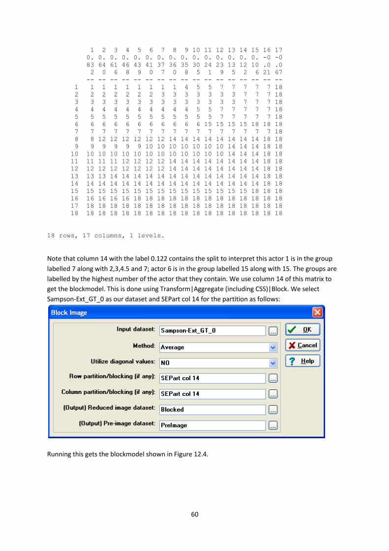
Note that column 14 with the label 0.122 contains the split to interpret this actor 1 is in the group

labelled 7 along with 2,3,4.5 and 7; actor 6 is in the group labelled 15 along with 15. The groups are

labelled by the highest number of the actor that they contain. We use column 14 of this matrix to

get the blockmodel. This is done using Transform|Aggregate (including CSS)|Block. We select

Sampson-Ext_GT_0 as our dataset and SEPart col 14 for the partition as follows:

Running this gets the blockmodel shown in Figure 12.4.

61

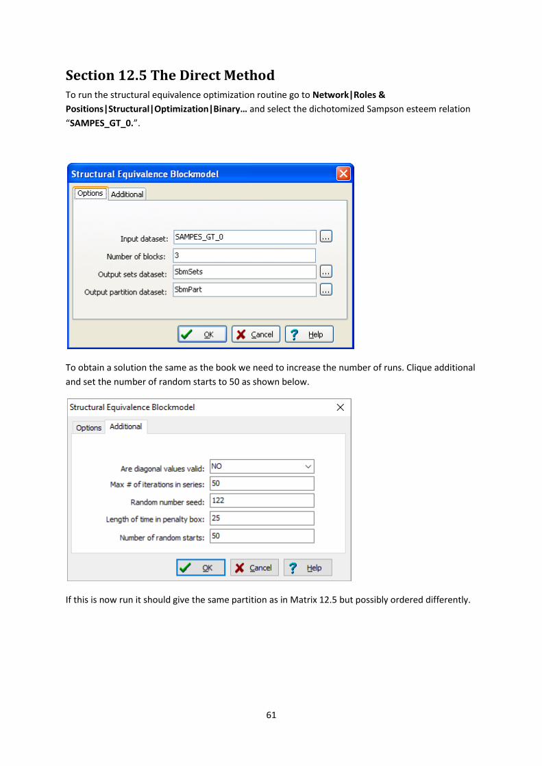
Section 12.5 The Direct Method To run the structural equivalence optimization routine go to Network|Roles &

Positions|Structural|Optimization|Binary… and select the dichotomized Sampson esteem relation

“SAMPES_GT_0.”.

To obtain a solution the same as the book we need to increase the number of runs. Clique additional

and set the number of random starts to 50 as shown below.

If this is now run it should give the same partition as in Matrix 12.5 but possibly ordered differently.

62

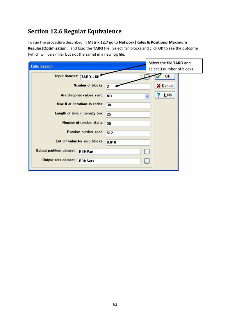
Section 12.6 Regular Equivalence

To run the procedure described in Matrix 12.7 go to Network|Roles & Positions|Maximum

Regular|Optimization… and load the TARO file. Select “3” blocks and click OK to see the outcome

(which will be similar but not the same) in a new log file.

Select the file TARO and

select 3 number of blocks

63

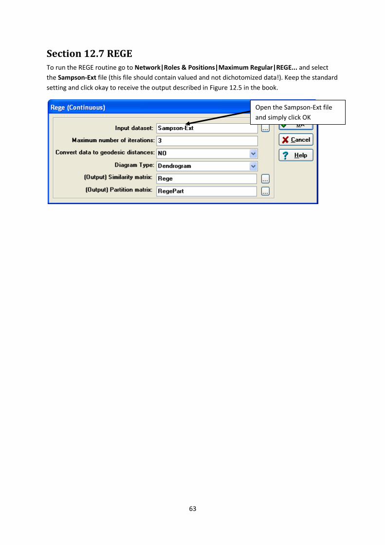
Section 12.7 REGE To run the REGE routine go to Network|Roles & Positions|Maximum Regular|REGE... and select

the Sampson-Ext file (this file should contain valued and not dichotomized data!). Keep the standard

setting and click okay to receive the output described in Figure 12.5 in the book.

Open the Sampson-Ext file

and simply click OK

64

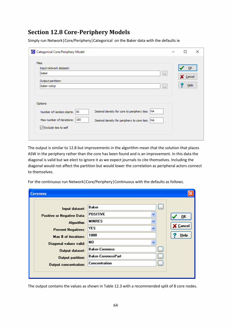
Section 12.8 Core-Periphery Models Simply run Network|Core/Periphery|Categorical on the Baker data with the defaults ie

The output is similar to 12.8 but improvements in the algorithm mean that the solution that places

ASW in the periphery rather than the core has been found and is an improvement. In this data the

diagonal is valid but we elect to ignore it as we expect journals to cite themselves. Including the

diagonal would not affect the partition but would lower the correlation as peripheral actors connect

to themselves.

For the continuous run Network|Core/Periphery|Continuous with the defaults as follows.

The output contains the values as shown in Table 12.3 with a recommended split of 8 core nodes.

65

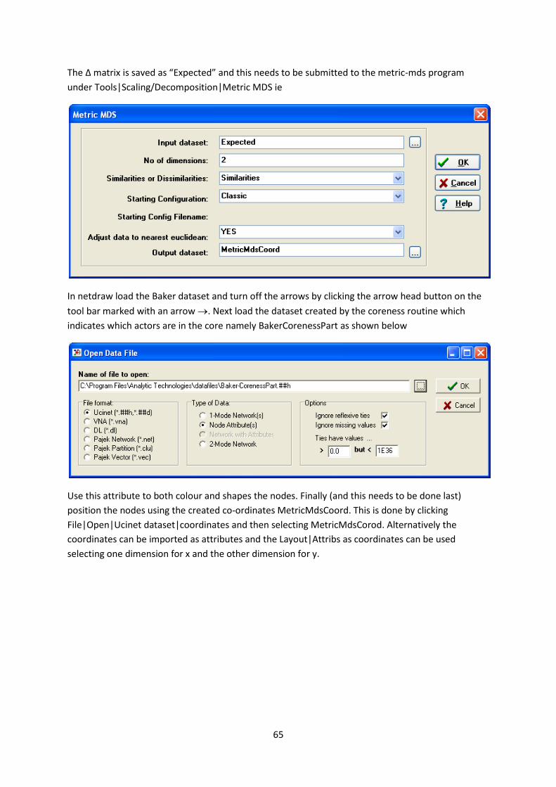
The Δ matrix is saved as “Expected” and this needs to be submitted to the metric-mds program

under Tools|Scaling/Decomposition|Metric MDS ie

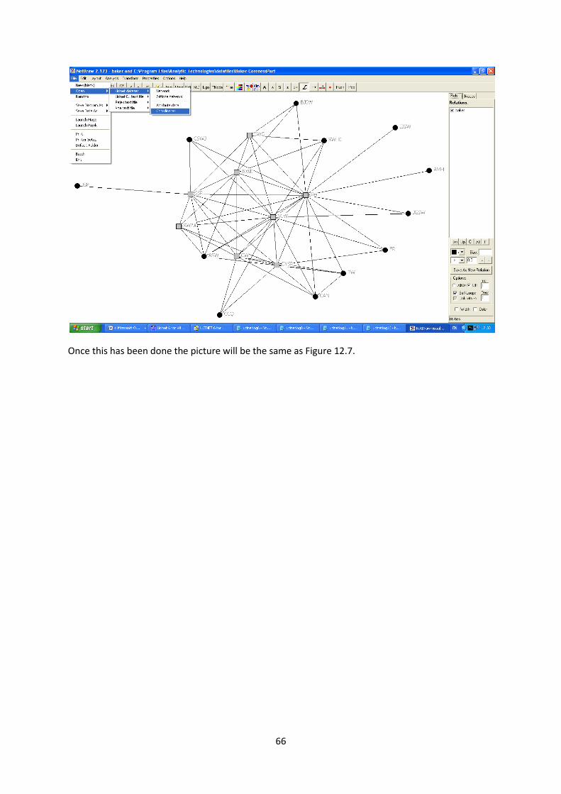
In netdraw load the Baker dataset and turn off the arrows by clicking the arrow head button on the

tool bar marked with an arrow . Next load the dataset created by the coreness routine which

indicates which actors are in the core namely BakerCorenessPart as shown below

Use this attribute to both colour and shapes the nodes. Finally (and this needs to be done last)

position the nodes using the created co-ordinates MetricMdsCoord. This is done by clicking

File|Open|Ucinet dataset|coordinates and then selecting MetricMdsCorod. Alternatively the

coordinates can be imported as attributes and the Layout|Attribs as coordinates can be used

selecting one dimension for x and the other dimension for y.

66

Once this has been done the picture will be the same as Figure 12.7.

67

Section 13.2 Converting to One-Mode Data

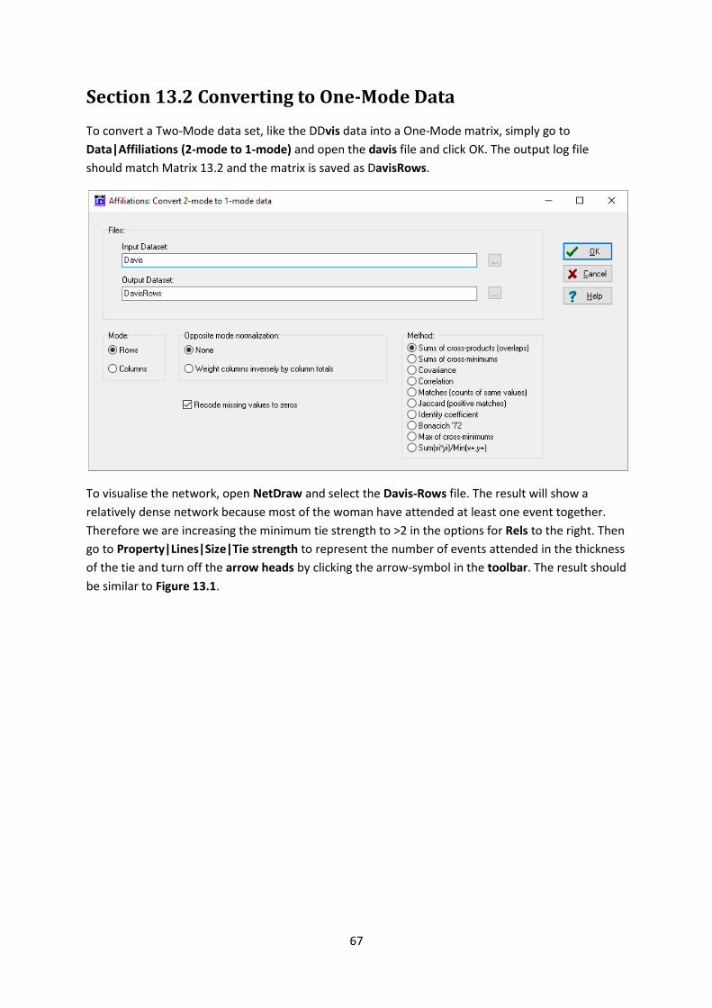
To convert a Two-Mode data set, like the DDvis data into a One-Mode matrix, simply go to

Data|Affiliations (2-mode to 1-mode) and open the davis file and click OK. The output log file

should match Matrix 13.2 and the matrix is saved as DavisRows.

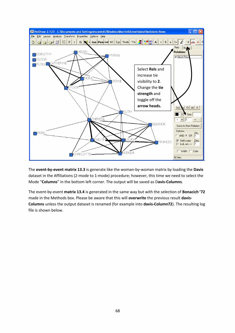
To visualise the network, open NetDraw and select the Davis-Rows file. The result will show a

relatively dense network because most of the woman have attended at least one event together.

Therefore we are increasing the minimum tie strength to >2 in the options for Rels to the right. Then

go to Property|Lines|Size|Tie strength to represent the number of events attended in the thickness

of the tie and turn off the arrow heads by clicking the arrow-symbol in the toolbar. The result should

be similar to Figure 13.1.

68

.

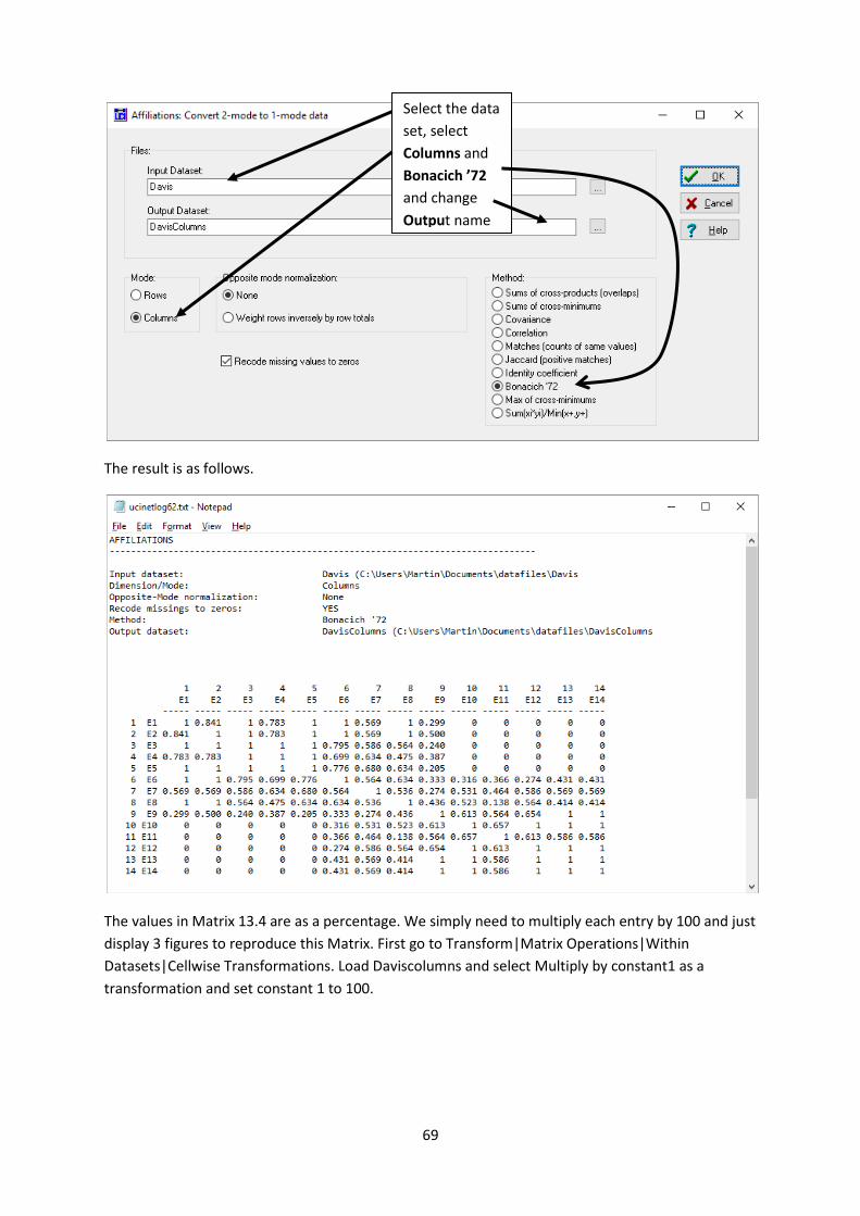
The event-by-event matrix 13.3 is generate like the woman-by-woman matrix by loading the Davis

dataset in the Affiliations (2-mode to 1-mode) procedure; however, this time we need to select the

Mode “Columns” in the bottom left corner. The output will be saved as Davis-Columns.

The event-by-event matrix 13.4 is generated in the same way but with the selection of Bonacich ’72

made in the Methods box. Please be aware that this will overwrite the previous result davis-

Columns unless the output dataset is renamed (for example into davis-Column72). The resulting log

file is shown below.

Select Rels and

increase tie

visibility to 2.

Change the tie

strength and

toggle off the

arrow heads.

69

The result is as follows.

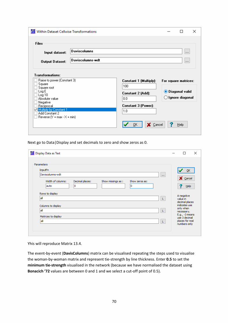
The values in Matrix 13.4 are as a percentage. We simply need to multiply each entry by 100 and just

display 3 figures to reproduce this Matrix. First go to Transform|Matrix Operations|Within

Datasets|Cellwise Transformations. Load Daviscolumns and select Multiply by constant1 as a

transformation and set constant 1 to 100.

Select the data

set, select

Columns and

Bonacich ’72

and change

Output name

70

Next go to Data|Display and set decimals to zero and show zeros as 0.

Yhis will reproduce Matrix 13.4.

The event-by-event (DavisColumns) matrix can be visualised repeating the steps used to visualise

the woman-by-woman matrix and represent tie-strength by line thickness. Enter 0.5 to set the

minimum tie-strength visualised in the network (because we have normalised the dataset using

Bonacich ’72 values are between 0 and 1 and we select a cut-off point of 0.5).

71

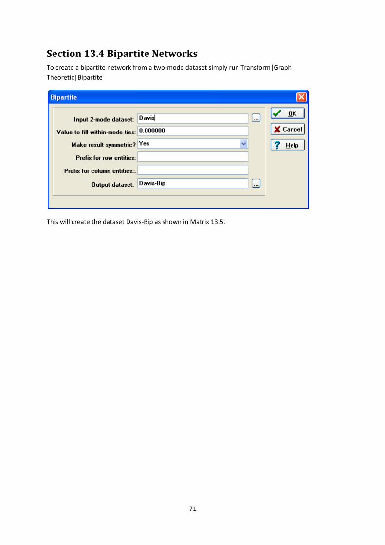
Section 13.4 Bipartite Networks To create a bipartite network from a two-mode dataset simply run Transform|Graph

Theoretic|Bipartite

This will create the dataset Davis-Bip as shown in Matrix 13.5.

72

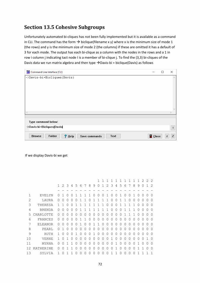
Section 13.5 Cohesive Subgroups

Unfortunately automated bi-cliques has not been fully implemented but it is available as a command

in CLI. The command has the form biclique(filename x y) where x is the minimum size of mode 1

(the rows) and y is the minimum size of mode 2 (the columns) if these are omitted it has a default of

3 for each mode. The output has each bi-clique as a column with the nodes in the rows and a 1 in

row i column j indicating tact node I is a member of bi-clique j. To find the (3,3) bi-cliques of the

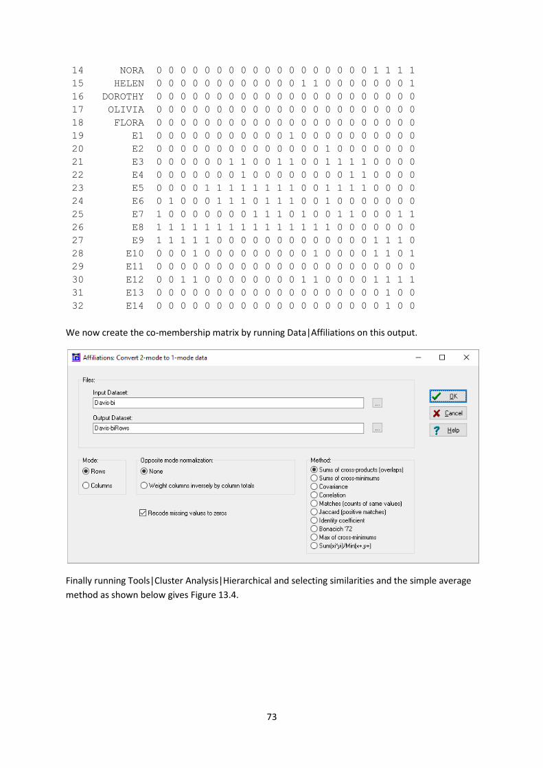
Davis data we run matrix algebra and then type Davis-bi = biclique(Davis) as follows

If we display Davis-bi we get

1 1 1 1 1 1 1 1 1 1 2 2 2

1 2 3 4 5 6 7 8 9 0 1 2 3 4 5 6 7 8 9 0 1 2

- - - - - - - - - - - - - - - - - - - - - -

1 EVELYN 0 1 0 0 1 1 1 1 0 0 0 1 0 0 1 0 0 1 0 0 0 0

2 LAURA 0 0 0 0 0 1 1 0 1 1 1 1 0 0 1 1 0 0 0 0 0 0

3 THERESA 1 1 0 0 1 1 1 1 1 1 1 0 0 0 1 1 1 1 0 0 0 0

4 BRENDA 0 0 0 0 0 1 1 1 1 1 1 1 0 0 0 1 1 1 0 0 0 0

5 CHARLOTTE 0 0 0 0 0 0 0 0 0 0 0 0 0 0 0 1 1 1 0 0 0 0

6 FRANCES 0 0 0 0 0 1 1 0 0 0 0 0 0 0 0 0 0 0 0 0 0 0

7 ELEANOR 0 0 0 0 0 1 0 0 1 1 0 0 0 0 0 0 0 0 0 0 0 0

8 PEARL 0 1 0 0 0 0 0 0 0 0 0 0 0 0 0 0 0 0 0 0 0 0

9 RUTH 1 0 0 0 1 0 0 0 1 0 0 0 0 0 0 0 0 0 0 0 0 0

10 VERNE 1 0 1 0 0 0 0 0 0 0 0 0 1 0 0 0 0 0 0 0 1 0

11 MYRNA 0 0 1 1 0 0 0 0 0 0 0 0 0 1 0 0 0 0 1 0 0 0

12 KATHERINE 0 0 1 1 0 0 0 0 0 0 0 0 0 1 0 0 0 0 1 1 0 0

13 SYLVIA 1 0 1 1 0 0 0 0 0 0 0 0 1 1 0 0 0 0 1 1 1 1

73

14 NORA 0 0 0 0 0 0 0 0 0 0 0 0 0 0 0 0 0 0 1 1 1 1

15 HELEN 0 0 0 0 0 0 0 0 0 0 0 0 1 1 0 0 0 0 0 0 0 1

16 DOROTHY 0 0 0 0 0 0 0 0 0 0 0 0 0 0 0 0 0 0 0 0 0 0

17 OLIVIA 0 0 0 0 0 0 0 0 0 0 0 0 0 0 0 0 0 0 0 0 0 0

18 FLORA 0 0 0 0 0 0 0 0 0 0 0 0 0 0 0 0 0 0 0 0 0 0

19 E1 0 0 0 0 0 0 0 0 0 0 0 1 0 0 0 0 0 0 0 0 0 0

20 E2 0 0 0 0 0 0 0 0 0 0 0 0 0 0 1 0 0 0 0 0 0 0

21 E3 0 0 0 0 0 0 1 1 0 0 1 1 0 0 1 1 1 1 0 0 0 0

22 E4 0 0 0 0 0 0 0 1 0 0 0 0 0 0 0 0 1 1 0 0 0 0

23 E5 0 0 0 0 1 1 1 1 1 1 1 1 0 0 1 1 1 1 0 0 0 0

24 E6 0 1 0 0 0 1 1 1 0 1 1 1 0 0 1 0 0 0 0 0 0 0

25 E7 1 0 0 0 0 0 0 0 1 1 1 0 1 0 0 1 1 0 0 0 1 1

26 E8 1 1 1 1 1 1 1 1 1 1 1 1 1 1 1 0 0 0 0 0 0 0

27 E9 1 1 1 1 1 0 0 0 0 0 0 0 0 0 0 0 0 0 1 1 1 0

28 E10 0 0 0 1 0 0 0 0 0 0 0 0 0 1 0 0 0 0 1 1 0 1

29 E11 0 0 0 0 0 0 0 0 0 0 0 0 0 0 0 0 0 0 0 0 0 0

30 E12 0 0 1 1 0 0 0 0 0 0 0 0 1 1 0 0 0 0 1 1 1 1

31 E13 0 0 0 0 0 0 0 0 0 0 0 0 0 0 0 0 0 0 0 1 0 0

32 E14 0 0 0 0 0 0 0 0 0 0 0 0 0 0 0 0 0 0 0 1 0 0

We now create the co-membership matrix by running Data|Affiliations on this output.

Finally running Tools|Cluster Analysis|Hierarchical and selecting similarities and the simple average

method as shown below gives Figure 13.4.

74

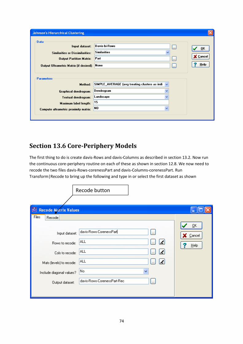
Section 13.6 Core-Periphery Models

The first thing to do is create davis-Rows and davis-Columns as described in section 13.2. Now run

the continuous core-periphery routine on each of these as shown in section 12.8. We now need to

recode the two files davis-Rows-corenessPart and davis-Columns-corenessPart. Run

Transform|Recode to bring up the following and type in or select the first dataset as shown

Recode button

75

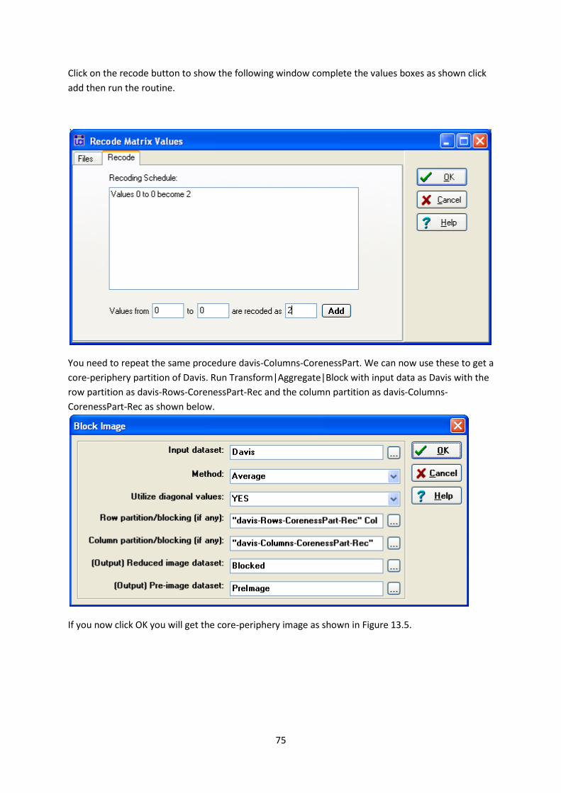
Click on the recode button to show the following window complete the values boxes as shown click

add then run the routine.

You need to repeat the same procedure davis-Columns-CorenessPart. We can now use these to get a

core-periphery partition of Davis. Run Transform|Aggregate|Block with input data as Davis with the

row partition as davis-Rows-CorenessPart-Rec and the column partition as davis-Columns-

CorenessPart-Rec as shown below.

If you now click OK you will get the core-periphery image as shown in Figure 13.5.

76

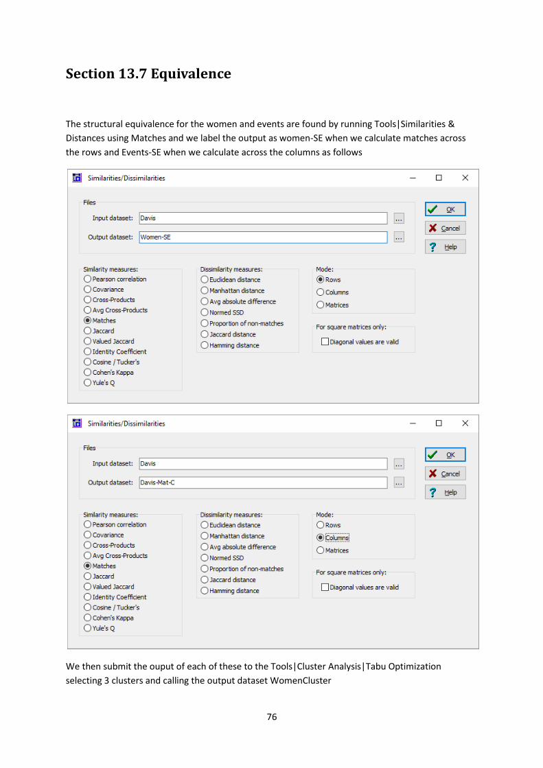
Section 13.7 Equivalence

The structural equivalence for the women and events are found by running Tools|Similarities &

Distances using Matches and we label the output as women-SE when we calculate matches across

the rows and Events-SE when we calculate across the columns as follows

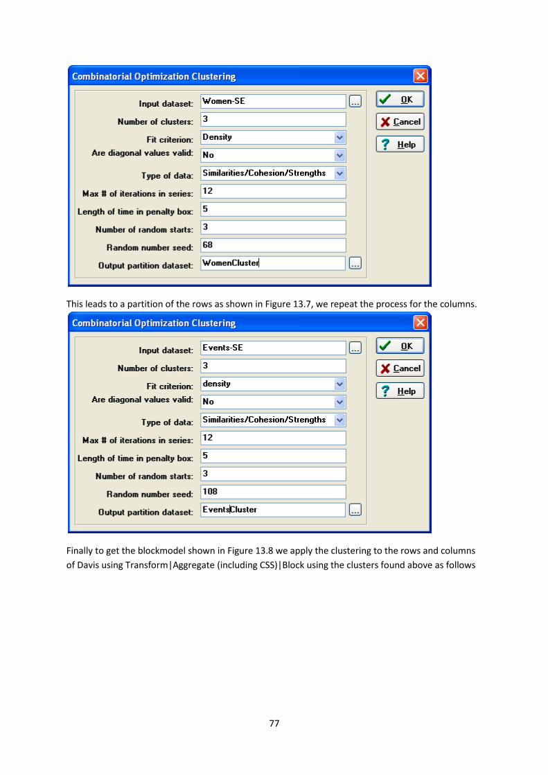
We then submit the ouput of each of these to the Tools|Cluster Analysis|Tabu Optimization

selecting 3 clusters and calling the output dataset WomenCluster

77

This leads to a partition of the rows as shown in Figure 13.7, we repeat the process for the columns.

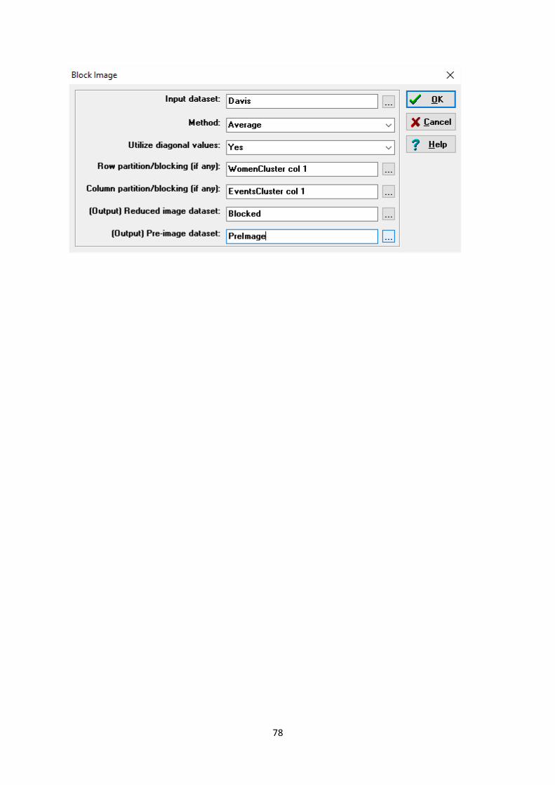
Finally to get the blockmodel shown in Figure 13.8 we apply the clustering to the rows and columns

of Davis using Transform|Aggregate (including CSS)|Block using the clusters found above as follows

78

79

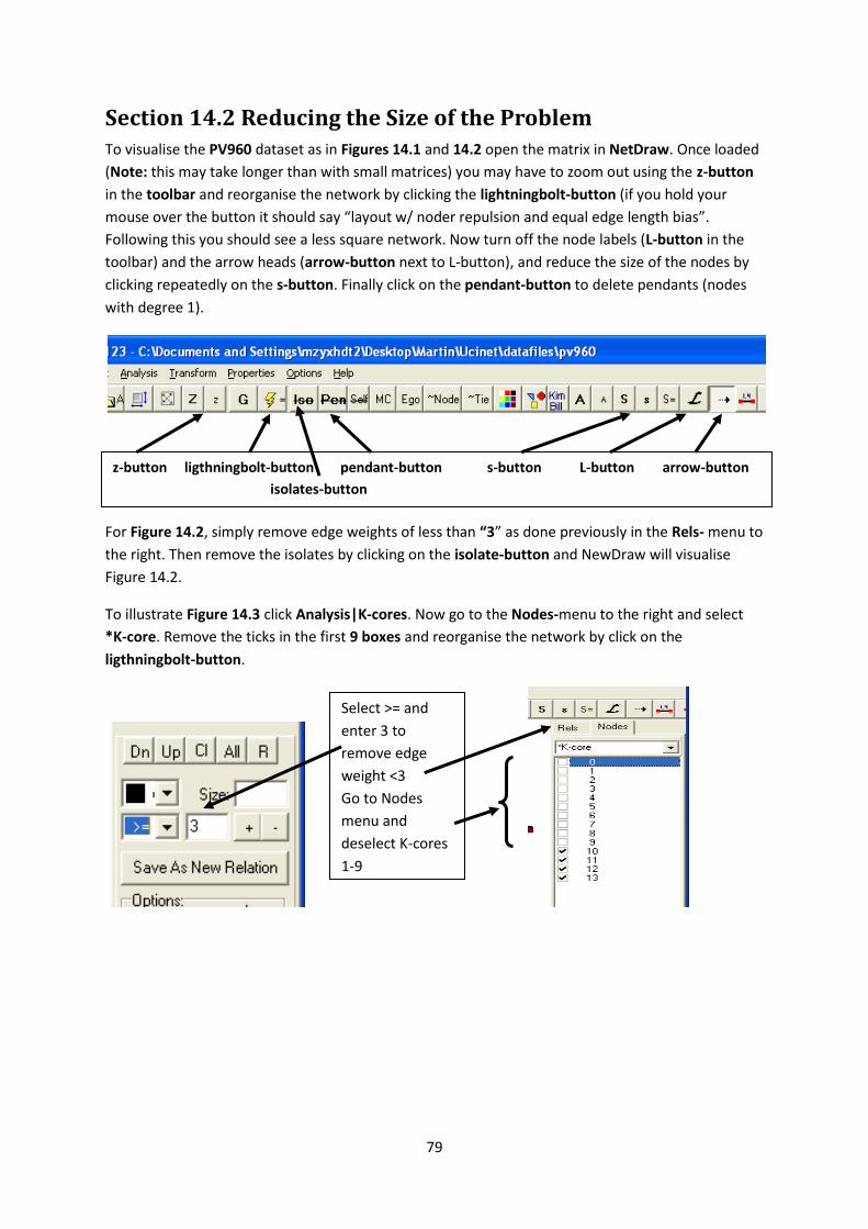
Section 14.2 Reducing the Size of the Problem To visualise the PV960 dataset as in Figures 14.1 and 14.2 open the matrix in NetDraw. Once loaded

(Note: this may take longer than with small matrices) you may have to zoom out using the z-button

in the toolbar and reorganise the network by clicking the lightningbolt-button (if you hold your

mouse over the button it should say “layout w/ noder repulsion and equal edge length bias”.

Following this you should see a less square network. Now turn off the node labels (L-button in the

toolbar) and the arrow heads (arrow-button next to L-button), and reduce the size of the nodes by

clicking repeatedly on the s-button. Finally click on the pendant-button to delete pendants (nodes

with degree 1).

For Figure 14.2, simply remove edge weights of less than “3” as done previously in the Rels- menu to

the right. Then remove the isolates by clicking on the isolate-button and NewDraw will visualise

Figure 14.2.

To illustrate Figure 14.3 click Analysis|K-cores. Now go to the Nodes-menu to the right and select

*K-core. Remove the ticks in the first 9 boxes and reorganise the network by click on the

ligthningbolt-button.

z-button ligthningbolt-button pendant-button s-button L-button arrow-button

isolates-button

Select >= and

enter 3 to

remove edge

weight <3

Go to Nodes

menu and

deselect K-cores

1-9

80

14.2.4 Aggregation

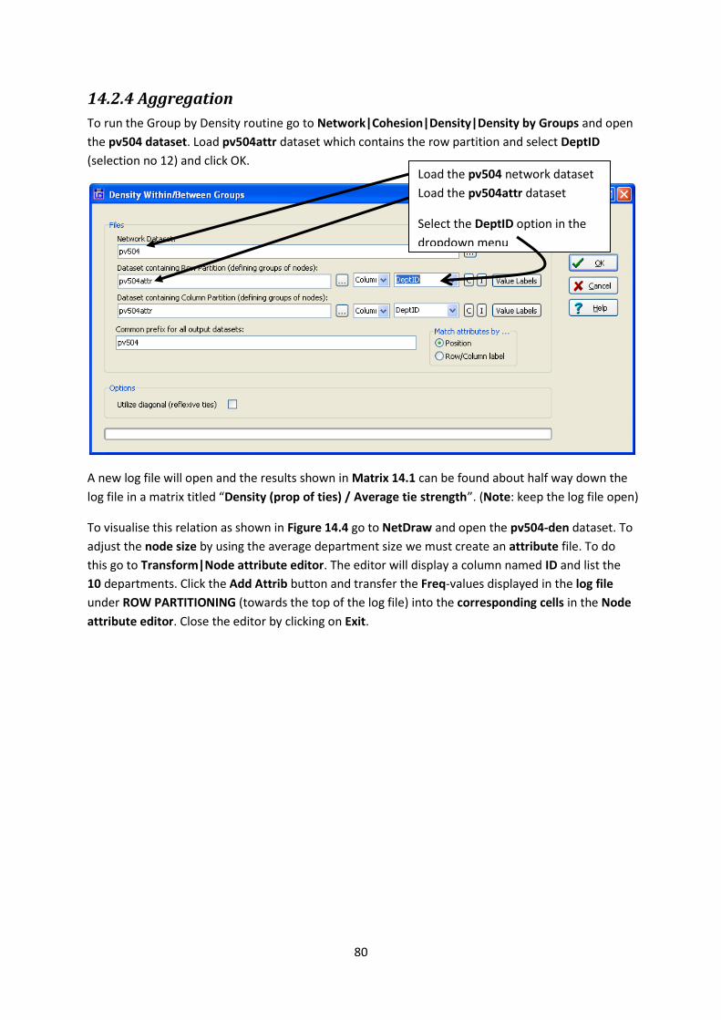
To run the Group by Density routine go to Network|Cohesion|Density|Density by Groups and open

the pv504 dataset. Load pv504attr dataset which contains the row partition and select DeptID

(selection no 12) and click OK.

A new log file will open and the results shown in Matrix 14.1 can be found about half way down the

log file in a matrix titled “Density (prop of ties) / Average tie strength”. (Note: keep the log file open)

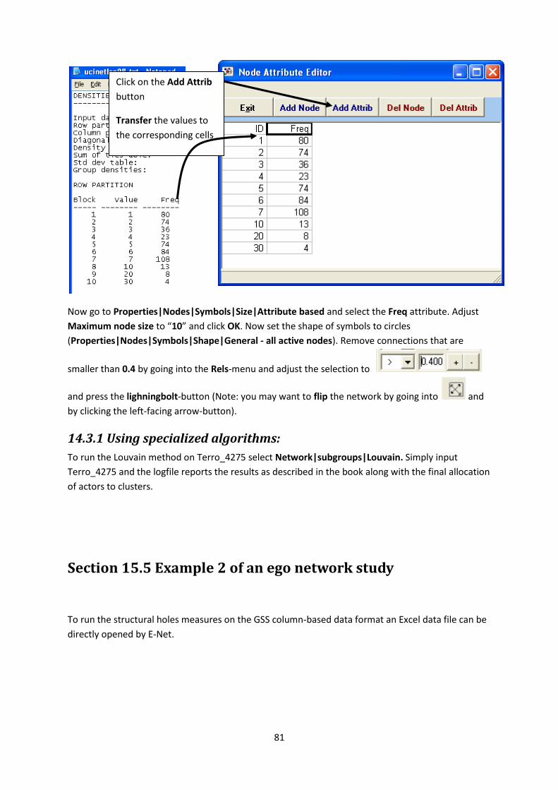
To visualise this relation as shown in Figure 14.4 go to NetDraw and open the pv504-den dataset. To

adjust the node size by using the average department size we must create an attribute file. To do

this go to Transform|Node attribute editor. The editor will display a column named ID and list the

10 departments. Click the Add Attrib button and transfer the Freq-values displayed in the log file

under ROW PARTITIONING (towards the top of the log file) into the corresponding cells in the Node

attribute editor. Close the editor by clicking on Exit.

Load the pv504 network dataset

Load the pv504attr dataset

Select the DeptID option in the

dropdown menu

81

Now go to Properties|Nodes|Symbols|Size|Attribute based and select the Freq attribute. Adjust

Maximum node size to “10” and click OK. Now set the shape of symbols to circles

(Properties|Nodes|Symbols|Shape|General - all active nodes). Remove connections that are

smaller than 0.4 by going into the Rels-menu and adjust the selection to

and press the lighningbolt-button (Note: you may want to flip the network by going into and

by clicking the left-facing arrow-button).

14.3.1 Using specialized algorithms:

To run the Louvain method on Terro_4275 select Network|subgroups|Louvain. Simply input

Terro_4275 and the logfile reports the results as described in the book along with the final allocation

of actors to clusters.

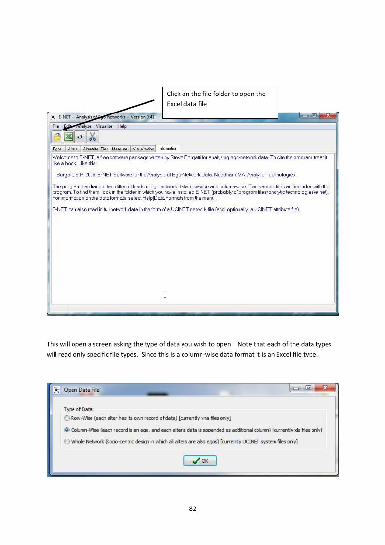
Section 15.5 Example 2 of an ego network study

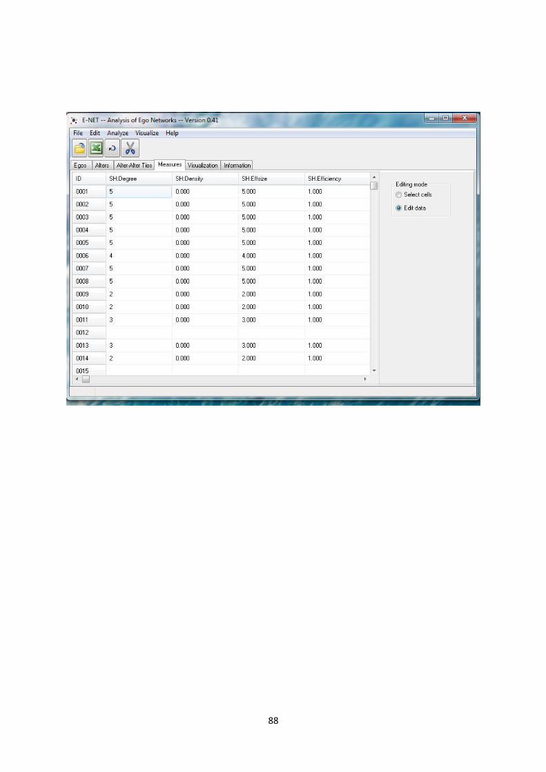
To run the structural holes measures on the GSS column-based data format an Excel data file can be

directly opened by E-Net.

Click on the Add Attrib

button

Transfer the values to

the corresponding cells

82

This will open a screen asking the type of data you wish to open. Note that each of the data types

will read only specific file types. Since this is a column-wise data format it is an Excel file type.

Click on the file folder to open the

Excel data file

83

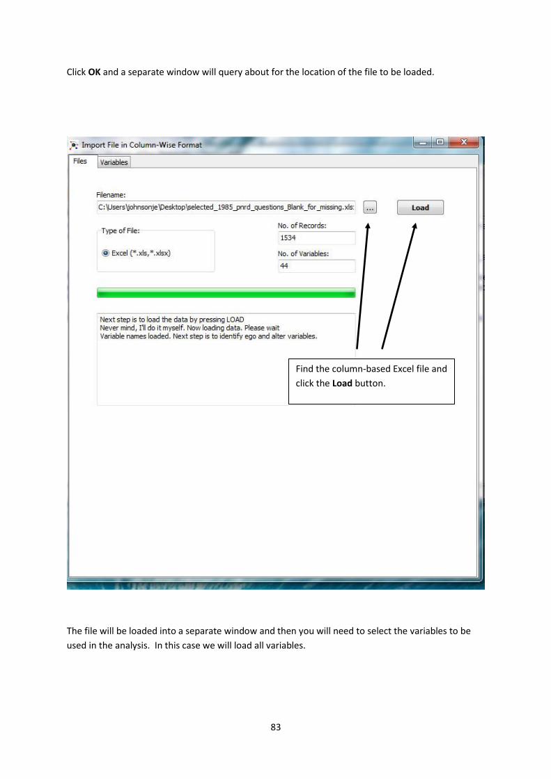
Click OK and a separate window will query about for the location of the file to be loaded.

The file will be loaded into a separate window and then you will need to select the variables to be

used in the analysis. In this case we will load all variables.

Find the column-based Excel file and

click the Load button.

84

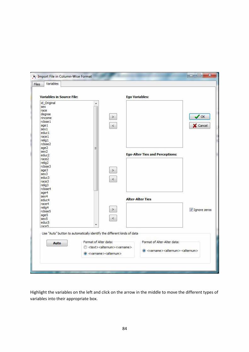
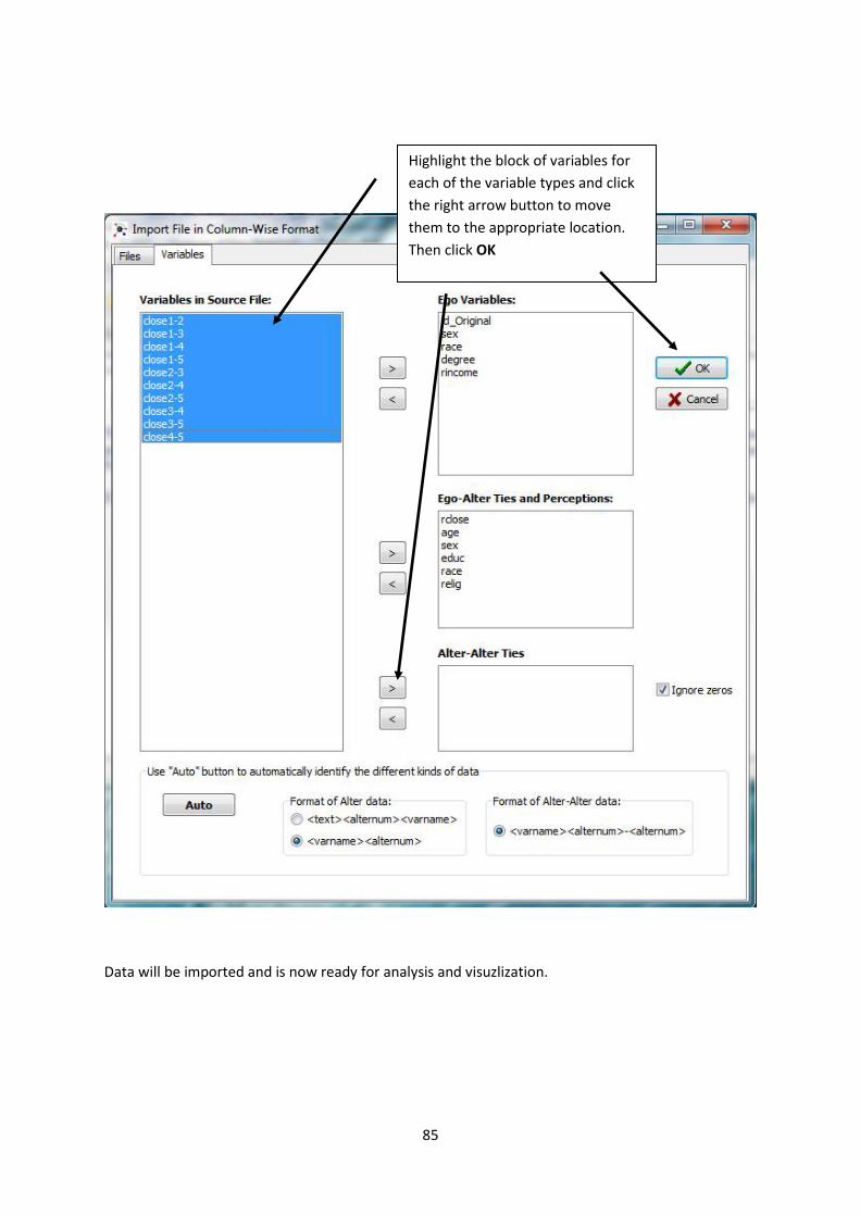
Highlight the variables on the left and click on the arrow in the middle to move the different types of

variables into their appropriate box.

85

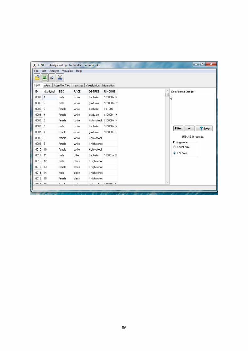
Data will be imported and is now ready for analysis and visuzlization.

Highlight the block of variables for

each of the variable types and click

the right arrow button to move

them to the appropriate location.

Then click OK

86

87

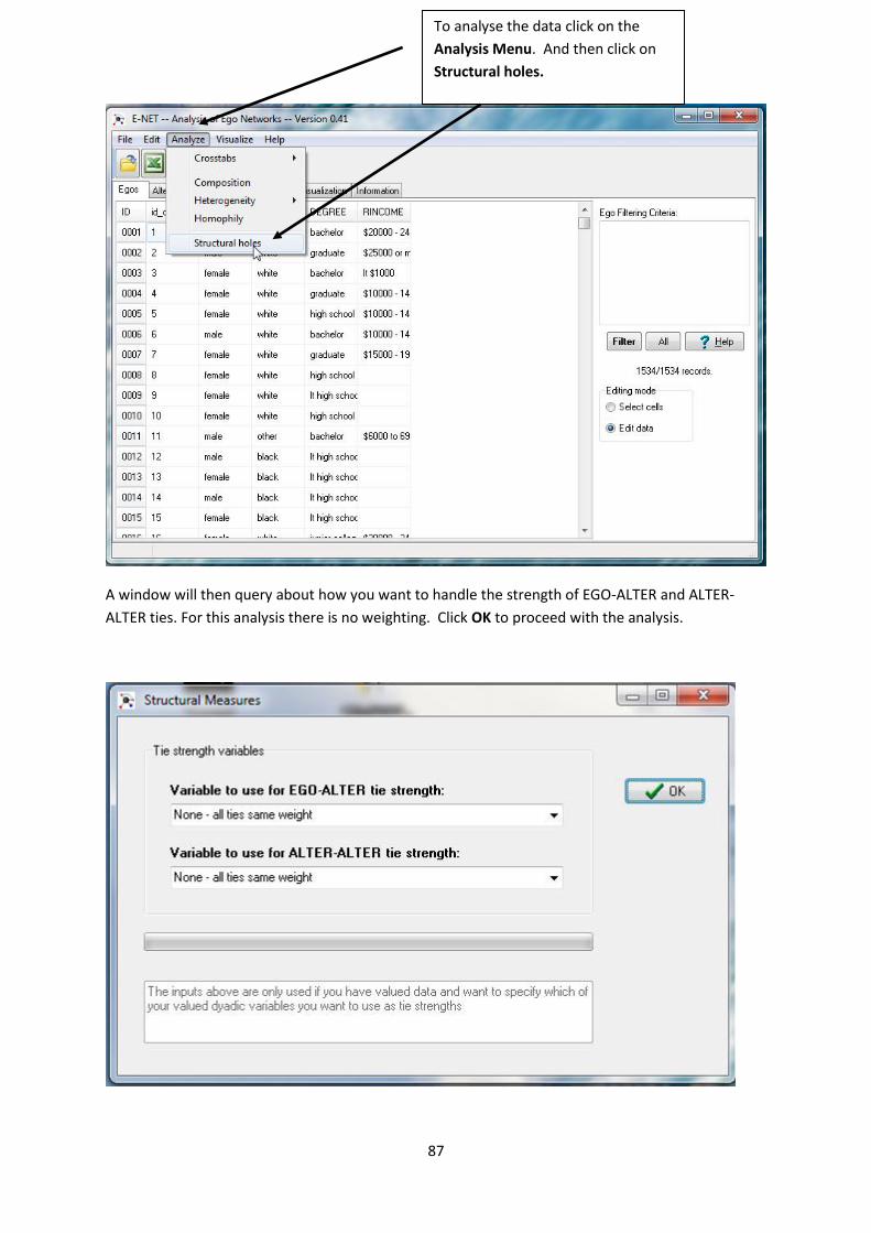
A window will then query about how you want to handle the strength of EGO-ALTER and ALTER-

ALTER ties. For this analysis there is no weighting. Click OK to proceed with the analysis.

To analyse the data click on the

Analysis Menu. And then click on

Structural holes.

88