Work Flexibility and Absenteeism: A Two-stageResidual Inclusion Approach

Ibrahima DialloPh.D. Student, Department of Economics-Universite Laval

ibrahima.diallo.11@ulaval.ca

April 29, 2021

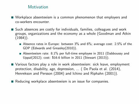
Workplace absenteeism is a common phenomenon that employers andco-workers encounter.

Such absences are costly for individuals, families, colleagues and workgroups, organizations and the economy as a whole (Goodman and Atkin(1984)).

Absence rates in Europe: between 3% and 6%; average cost: 2.5% of theGDP (Edwards and Greasley(2010)).

Absenteeism rate: 8.1% per full-time employee in 2011 (Dabboussy andUppal(2012); cost: $16.6 billion in 2011 (Stewart (2013)).

Various factors play a role in work absenteeism: sick leave, employmentprotection, disability, age, depression, ... ( De Paola et al. (2014),Henrekson and Persson (2004) and Ichino and Riphahn (2001)).

Reducing workplace absenteeism is an issue for companies.

2

Motivation

In recent years there has been growing interest in flexibility at work

71.2% (very likely) 10.8% (already in FWA) ( Employment and SocialDevelopment Canada, (2016)

Top benefits of work flexibility

Improve employee work live balancePositive impact on staff engagement and motivation (Casper and Buffardi,2004)improve worker health, through reduced stress and increased jobsatisfaction (Possenriede, 2011).

Studies to date on the relationship between employment flexibility andwork absence show an ambiguous effect

Some forms of flexibility (working regular hours, working on theweekend, working at home, and working a reduced work week) decreaseabsence, and other form like working flexible hours,workingnontraditional hours, working in a shift, and working a compressed workweek actually increase absence (Heywood and Miller (2015), Casey andGrzywacz, 2008, Dionne and Dostie (2007))

3

Motivation

1 We study the impact of work flexibility on the probability of missing aworkweeks.

2 We use the Survey of Labour and Income Dynamics to analyze theeffects of working at home and part time work on absenteeism due toillness or personal/family reasons.

3 We use a variant of the instrumental variables method adapted tononlinear models (2SRI) to take account for the potential endogeneity ofworking at home.

4

This paper

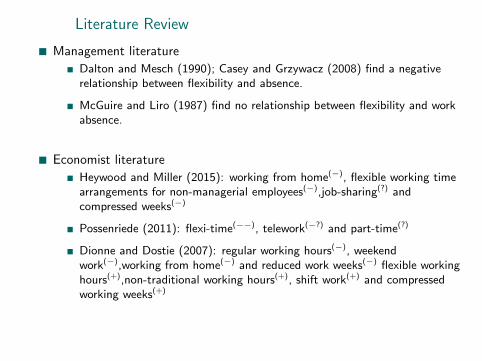
Management literature

Dalton and Mesch (1990); Casey and Grzywacz (2008) find a negativerelationship between flexibility and absence.

McGuire and Liro (1987) find no relationship between flexibility and workabsence.

Economist literature

Heywood and Miller (2015): working from home(−), flexible working timearrangements for non-managerial employees(−),job-sharing(?) andcompressed weeks(−)

Possenriede (2011): flexi-time(−−), telework(−?) and part-time(?)

Dionne and Dostie (2007): regular working hours(−), weekendwork(−),working from home(−) and reduced work weeks(−) flexible workinghours(+),non-traditional working hours(+), shift work(+) and compressedworking weeks(+)

5

Literature Review

1 Data

2 Empirical specification

3 Results

4 Conclusion

6

Road Map

1 Data

2 Empirical specification

3 Results

4 Conclusion

7

Outline

Canadian’s Survey of Labor and Income Dynamics (SLID)

Longitudinal overlapping panel data on panel 3 to 6.

We exploit the section on absences from work

Information on absence from work, work from home, part time, health status,socio-demographic characteristics, job characteristics and industry.

Sample restrictions

Age: 18-65;Employment : only employed workers (Workers that are unemployed ornot in labour market for part or all the period are excluded);We consider workers that are stayed in the same job during the period;We disregard individuals that have changed their region;

8

Data

Table: Descritptive statitics

Variables Mean Median St.dev N

Workweeks missed 7.9665 4 9.5603 20,757Home work 0.0684 0 0.2524 20,757Part time 0.2003 0 0.4002 20,757Female 0.5644 1 0.4958 20,757Handicap 0.2214 0 0.4152 20,757Age 41.2574 42 11.6463 20,757Wage 18.7181 17.5 7.4843 20,757Under secondary education 0.1353 0 0.3421 20,757Secondary education 0.3098 0 0.4624 20,757Higher education 0.5548 1 0.4970 20,757Married 0.6203 1 0.4853 20,757Household size 2.9394 3 1.3739 20,757Children (0-5 years) 0.1770 0 0.4896 20,757Children (6-17 years) 0.4997 0 0.8585 20,757

Sources: SLID panels 3 to 6 and author calculation.

9

Descriptive statistics

Table: Descritptive statitics

Variables Mean Median St.dev N

Public sector 0.2948 0 0.4560 20,757Union member 0.4715 0 0.4992 20,757Number of employerLess than 20 0.2665 0 0.4421 20,75720 to 99 0.3138 0 0.4640 20,757100 to 499 0.2522 0 0.4343 20,757500 to 999 0.0692 0 0.2539 20,7571000 and over 0.0981 0 0.2975 20,757Paid during absence 0.4744 0 0.4994 20,757Regular shift 0.7401 1 0.4386 20,757Profit sharing 0.0738 0 0.2614 20,757Supervision 0.2673 0 0.4426 21,847

Sources: SLID panels 3 to 6 and author calculation.

10

Descriptive statistics

1 Data

2 Empirical specification

3 Results

4 Conclusion

11

Outline

We models decision to miss workweek

Let U0i the utility of not missing a workweek and U1i the utility ofmissing a workweek

U0i = x′iβ0 + ε0i (1)

U1i = x′iβ1 + ε1i (2)

Individual i misses a workweek at period t if

U1i > U0i =⇒ ε0i − ε1i < x’i (β1 − β0) (3)

Let

yi =

{1 if U1i > U0i

0 otherwise=⇒ Standard binary outcome model (4)

With random repeated events of the same kind the distribution of thenumber of success is Poisson distribution (Cameron and Trived (2013))

12

Econometric model

The estimation method use the 2SRI approach (Terza et al. (2008))

Let mi be the number of workweeks missed. mi ∼ Poiss(µi )

µi = E (mi |fi , xi , ui ) = exp(β1fi + x’1iβ3 + ui ) (5)

where ui = ϕεi + νi , νi is i.i.d, independent of εi , and E [evi ] = cst

1 First stage: Estimate a Probit regression and obtain residuals

Let fi be the dummy variable equal 1 if workers hold a flexible job and 0otherwise

fi = φ(x’2iγ) + ri (6)

We use provincial variation as instrumental variables

2 Second stage: Estimate Poisson including the residual obtained in thefirst stage

µi = E (mi |fi , xi , ui ) = exp(β1fi + x’1iβ2 + ϕri + νi ) (7)

13

Estimation procedure

1 Data

2 Empirical specification

3 Results

4 Conclusion

14

Outline

Table: Standard Poisson and Two stage residual inclusion approach

Poisson 2SRIVariables Pooled Panel Pooled PanelJob flexibility (1=yes; 0=no)Work at home -0.0173*** -0.0747*** -0.0167*** -0.0683***

(0.000353) (0.000862) (0.000372) (0.000923)Part time -0.0283*** 0.0750*** -0.0283*** 0.0750***

(0.000228) (0.000597) (0.000228) (0.000597)Handicap (1=yes; 0=no) 0.539*** 0.333*** 0.539*** 0.333***

(0.000178) (0.000392) (0.000178) (0.000392)Gender (1=female, 0=male) 0.0690*** 0.0807*** 0.0690*** 0.0806***

(0.000209) (0.000970) (0.000209) (0.000970)Residuals 4.37e-05*** 0.000434***

(8.17e-06) (2.27e-05)Observations 20,757 10,467 20,757 10,467Number of id 4,961 4,961

Note: Poisson regression model and 2SRI approach for relationship between job flexibility and absences from work with control for individualcharacteristics and firms. Standard errors in parentheses ∗∗∗p < 0.01, ∗∗p < 0.05, ∗p < 0.1

All Results

15

Results

Table: Robustness check

Interaction Misclassification errorsVariables Negative Binomial Poisson Negative binomial Poisson Negative binomialJob flexibility (1=yes; 0=no)Work at home -0.0241*** -0.0667*** -0.0514*** -0.0756*** -0.0672***

(0.00104) (0.000657) (0.00170) (0.000650) (0.00168)Part time -0.0238*** -0.0280*** -0.0234*** -0.0218*** -0.0181***

(0.000650) (0.000228) (0.000650) (0.000224) (0.000638)Handicap (1=yes; 0=no) 0.548*** 0.584*** 0.592*** 0.578*** 0.588***

(0.000561) (0.000679) (0.00211) (0.000677) (0.00211)Gender (1=female, 0=male) 0.0758*** 0.115*** 0.0979*** 0.133*** 0.121***

(0.000583) (0.000698) (0.00190) (0.000689) (0.0018)Handicap×Work at home -0.048*** -0.048*** -0.0467*** -0.0482***

(0.0007) (0.0021) (0.000701) (0.00218)Gender×Work at home -0.050*** -0.024*** -0.0678*** 0.0502***

(0.0007) (0.0020) (0.000710) (0.00194)Residuals -0.000113*** -2.03e-06 -0.000148*** -0.00500*** -0.00584***

(2.43e-05) (8.16e-06) (2.44e-05) (6.19e-05) (0.000204)lnalpha -0.133*** -0.133*** -0.127***

(0.000359) (0.000359) (0.000358)Observations 20,757 20,757 20,757 20,757 20,757

Standard errors in parentheses ∗∗∗p < 0.01, ∗∗p < 0.05, ∗p < 0.1

16

Results

1 Data

2 Empirical specification

3 Results

4 Conclusion

17

Outline

We examined the association between job flexibility and job absencesafter controlling for individual and firm characteristics.

We defined two forms of flexibility: working at home and part-time.

We recognize that there is some geographical variation in the ability tooffer flexibility, we use an instrumental variables approach to explore thispotential source of bias.

We then performed checks for overdispersion, heterogeneity, andmisclassification which showed significant interaction effects whileconfirming the importance of flexibility.

18

Conclusion

THANK YOUANY QUESTIONS

19

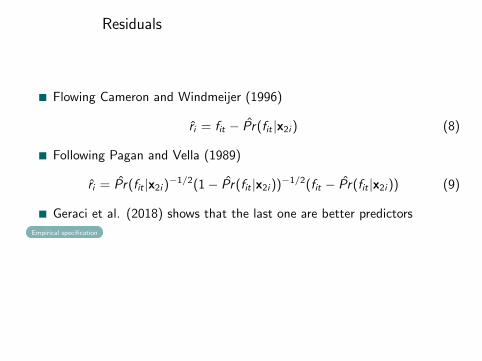
Flowing Cameron and Windmeijer (1996)

ri = fit − Pr(fit |x2i ) (8)

Following Pagan and Vella (1989)

ri = Pr(fit |x2i )−1/2(1− Pr(fit |x2i ))−1/2(fit − Pr(fit |x2i )) (9)

Geraci et al. (2018) shows that the last one are better predictors

Empirical specification

20

Residuals

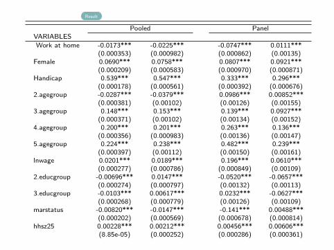
Pooled PanelVARIABLES

Work at home -0.0173*** -0.0225*** -0.0747*** 0.0111***(0.000353) (0.000982) (0.000862) (0.00135)

Female 0.0690*** 0.0758*** 0.0807*** 0.0921***(0.000209) (0.000583) (0.000970) (0.000871)

Handicap 0.539*** 0.547*** 0.333*** 0.296***(0.000178) (0.000561) (0.000392) (0.000676)

2.agegroup -0.0287*** -0.0379*** 0.0986*** 0.00852***(0.000381) (0.00102) (0.00126) (0.00155)

3.agegroup 0.148*** 0.153*** 0.139*** 0.0927***(0.000371) (0.00102) (0.00134) (0.00152)

4.agegroup 0.200*** 0.201*** 0.263*** 0.136***(0.000356) (0.000983) (0.00136) (0.00147)

5.agegroup 0.224*** 0.238*** 0.482*** 0.239***(0.000397) (0.00112) (0.00150) (0.00161)

lnwage 0.0201*** 0.0189*** 0.196*** 0.0610***(0.000277) (0.000786) (0.000849) (0.00109)

2.educgroup -0.00696*** 0.0147*** -0.0520*** -0.0657***(0.000274) (0.000797) (0.00132) (0.00113)

3.educgroup -0.0103*** 0.00617*** 0.0232*** -0.0627***(0.000268) (0.000779) (0.00126) (0.00109)

marstatus -0.00820*** -0.0147*** -0.141*** 0.00488***(0.000202) (0.000569) (0.000678) (0.000814)

hhsz25 0.00228*** 0.00212*** 0.00456*** 0.00606***(8.85e-05) (0.000252) (0.000286) (0.000361)

21

Result

Pooled PanelVARIABLES

children 0 5 0.116*** 0.114*** 0.108*** 0.0665***(0.000194) (0.000558) (0.000602) (0.000808)

children 6 17 -0.000327** -0.00364*** 0.0576*** 0.00933***(0.000134) (0.000386) (0.000432) (0.000538)

Public sector 0.0701*** 0.0881*** 0.0233*** -0.0164***(0.000232) (0.000666) (0.000881) (0.000922)

Union member 0.136*** 0.128*** 0.143*** 0.147***(0.000210) (0.000594) (0.000676) (0.000828)

2.nbempl2 0.0433*** 0.0421*** 0.0190*** 0.0527***(0.000229) (0.000636) (0.000638) (0.000894)

3.nbempl2 0.0751*** 0.0857*** 0.0737*** 0.0706***(0.000249) (0.000707) (0.000705) (0.000960)

4.nbempl2 0.0522*** 0.0419*** -0.0741*** 0.000830(0.000373) (0.00106) (0.000899) (0.00139)

5.nbempl2 0.142*** 0.129*** -0.0145*** 0.0985***(0.000331) (0.000960) (0.000874) (0.00125)

pai abs -0.229*** -0.255*** -0.251*** -0.147***(0.000187) (0.000535) (0.000421) (0.000690)

Part time -0.0283*** -0.0238*** 0.0750*** -0.0163***(0.000228) (0.000650) (0.000597) (0.000896)

shift -0.0366*** -0.0356*** -0.0338*** 0.00930***(0.000196) (0.000560) (0.000497) (0.000751)

pishare -0.0119*** 0.0112*** 0.0867*** 0.0395***(0.000338) (0.000933) (0.000751) (0.00122)

supervision -0.152*** -0.149*** -0.113*** -0.0698***(0.000206) (0.000562) (0.000484) (0.000758)

Constant 1.825*** 1.800*** 1.359*** 0.134***(0.000990) (0.00279) (0.00321) (0.00397)

Observations 20,757 20,757 10,467 10,4674,961 4,961

22

Result