Word2vec embeddings: CBOW and Skipgram · Word2vec embeddings: CBOW and Skipgram VL Embeddings Uni...
77
Skipgram – Intuition Gradient Descent Stochastic Gradient Descent Backpropagation Word2vec embeddings: CBOW and Skipgram VL Embeddings Uni Heidelberg SS 2019
Transcript of Word2vec embeddings: CBOW and Skipgram · Word2vec embeddings: CBOW and Skipgram VL Embeddings Uni...

Skipgram – Intuition Gradient Descent Stochastic Gradient Descent Backpropagation
Word2vec embeddings: CBOW and Skipgram
VL Embeddings
Uni Heidelberg
SS 2019
Skipgram – Intuition Gradient Descent Stochastic Gradient Descent Backpropagation
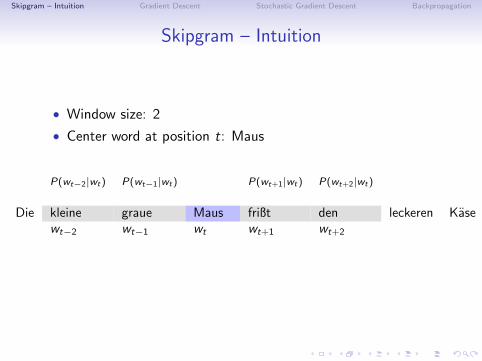
Skipgram – Intuition
• Window size: 2
• Center word at position t: Maus
P(wt−2|wt) P(wt−1|wt) P(wt+1|wt) P(wt+2|wt)
Die kleine graue Maus frißt den leckeren Kasewt−2 wt−1 wt wt+1 wt+2
Same probability distribution used for all context words

Skipgram – Intuition Gradient Descent Stochastic Gradient Descent Backpropagation
Skipgram – Intuition
• Window size: 2
• Center word at position t: frißt
P(wt−2|wt) P(wt−1|wt) P(wt+1|wt) P(wt+2|wt)
Die kleine graue Maus frißt den leckeren Kasewt−2 wt−1 wt wt+1 wt+2
Same probability distribution used for all context words

Skipgram – Intuition Gradient Descent Stochastic Gradient Descent Backpropagation
Skipgram – Intuition
• Window size: 2
• Center word at position t:
P(wt−2|wt) P(wt−1|wt) P(wt+1|wt) P(wt+2|wt)
Die kleine graue Maus frißt den leckeren Kasewt−2 wt−1 wt wt+1 wt+2
Same probability distribution used for all context words

Skipgram – Intuition Gradient Descent Stochastic Gradient Descent Backpropagation
Skipgram – Objective function
For each position t = 1, ...,T , predict context words within awindow of fixed size m, given center word wj .
L(θ) =T∏t=1
∏−m≤j≤m
P(wt+j |wt ; θ) (1)Likelihood =
j 6= 0 What is θ?
J(θ) = − 1
Tlog L(θ) = − 1
T
T∑t=1
∑−m≤j≤m
log P(wt+j |wt ; θ) (2)
j 6= 0
Minimising objective function ⇔ maximising predictive accuracy

Skipgram – Intuition Gradient Descent Stochastic Gradient Descent Backpropagation
Skipgram – Objective function
For each position t = 1, ...,T , predict context words within awindow of fixed size m, given center word wj .
L(θ) =T∏t=1
∏−m≤j≤m
P(wt+j |wt ; θ) (1)Likelihood =
j 6= 0 θ: vector representationsof each word
J(θ) = − 1
Tlog L(θ) = − 1
T
T∑t=1
∑−m≤j≤m
log P(wt+j |wt ; θ) (2)
j 6= 0
Minimising objective function ⇔ maximising predictive accuracy
Skipgram – Intuition Gradient Descent Stochastic Gradient Descent Backpropagation
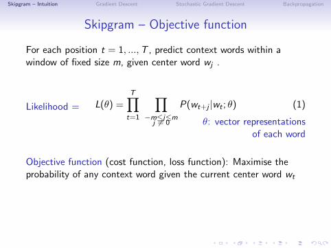
Skipgram – Objective function
For each position t = 1, ...,T , predict context words within awindow of fixed size m, given center word wj .
L(θ) =T∏t=1
∏−m≤j≤m
P(wt+j |wt ; θ) (1)Likelihood =
j 6= 0 θ: vector representationsof each word
Objective function (cost function, loss function): Maximise theprobability of any context word given the current center word wt
J(θ) = − 1
Tlog L(θ) = − 1
T
T∑t=1
∑−m≤j≤m
log P(wt+j |wt ; θ) (2)
j 6= 0
Minimising objective function ⇔ maximising predictive accuracy
Skipgram – Intuition Gradient Descent Stochastic Gradient Descent Backpropagation
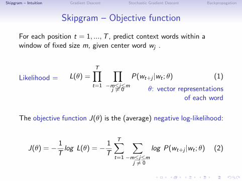
Skipgram – Objective function
For each position t = 1, ...,T , predict context words within awindow of fixed size m, given center word wj .
L(θ) =T∏t=1
∏−m≤j≤m
P(wt+j |wt ; θ) (1)Likelihood =
j 6= 0 θ: vector representationsof each word
The objective function J(θ) is the (average) negative log-likelihood:(cost function, loss function)
J(θ) = − 1
Tlog L(θ) = − 1
T
T∑t=1
∑−m≤j≤m
log P(wt+j |wt ; θ) (2)
j 6= 0
Minimising objective function ⇔ maximising predictive accuracy

Skipgram – Intuition Gradient Descent Stochastic Gradient Descent Backpropagation
Skipgram – Objective function
For each position t = 1, ...,T , predict context words within awindow of fixed size m, given center word wj .
L(θ) =T∏t=1
∏−m≤j≤m
P(wt+j |wt ; θ) (1)Likelihood =
j 6= 0 θ: vector representationsof each word
The objective function J(θ) is the (average) negative log-likelihood:(cost function, loss function)
J(θ) = − 1
Tlog L(θ) = − 1
T
T∑t=1
∑−m≤j≤m
log P(wt+j |wt ; θ) (2)
j 6= 0
Minimising objective function ⇔ maximising predictive accuracy
Skipgram – Intuition Gradient Descent Stochastic Gradient Descent Backpropagation
Objective function – Motivation
• We want to model the probability distribution over mutuallyexclusive classes• measure the difference between predicted probabilities y and
ground-truth probabilities y• during training: tune parameters so that this difference is
minimised
Skipgram – Intuition Gradient Descent Stochastic Gradient Descent Backpropagation
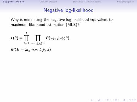
Negative log-likelihood
Why is minimising the negative log likelihood equivalent tomaximum likelihood estimation (MLE)?
L(θ) =T∏t=1
∏−m≤j≤m
P(wt+j |wt ; θ)
MLE = argmax L(θ, x)
• The log allows us to convert a product of factors into asummation of factors (nicer mathematical properties)
• arg maxx
(x) is equivalent to arg minx
(−x)
J(θ) = − 1T log L(θ) = − 1
T
T∑t=1
∑−m≤j≤m
log P(wt+j |wt ; θ)

Skipgram – Intuition Gradient Descent Stochastic Gradient Descent Backpropagation
Negative log-likelihood
Why is minimising the negative log likelihood equivalent tomaximum likelihood estimation (MLE)?
L(θ) =T∏t=1
∏−m≤j≤m
P(wt+j |wt ; θ)
MLE = argmax L(θ, x)
• The log allows us to convert a product of factors into asummation of factors (nicer mathematical properties)
• arg maxx
(x) is equivalent to arg minx
(−x)
J(θ) = − 1T log L(θ) = − 1
T
T∑t=1
∑−m≤j≤m
log P(wt+j |wt ; θ)
Skipgram – Intuition Gradient Descent Stochastic Gradient Descent Backpropagation
Negative log-likelihood
• We can interpret negative log-probability as informationcontent or surprisal
What is the log-likelihood of a model, given an event?
⇒ The negative of the surprisal of the event, given the model:A model is supported by an event to the extent that the eventis unsurprising, given the model.
Skipgram – Intuition Gradient Descent Stochastic Gradient Descent Backpropagation
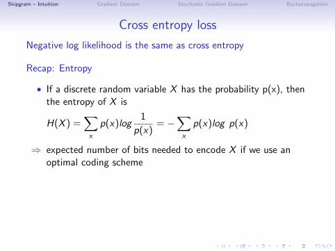
Cross entropy loss
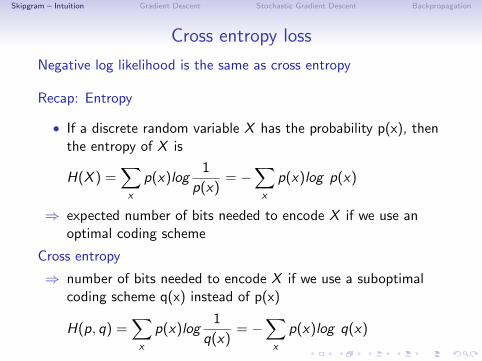
Negative log likelihood is the same as cross entropy
Recap: Entropy
• If a discrete random variable X has the probability p(x), thenthe entropy of X is
H(X ) =∑x
p(x)log1
p(x)= −
∑x
p(x)log p(x)
⇒ expected number of bits needed to encode X if we use anoptimal coding scheme
Cross entropy
⇒ number of bits needed to encode X if we use a suboptimalcoding scheme q(x) instead of p(x)
H(p, q) =∑x
p(x)log1
q(x)= −
∑x
p(x)log q(x)
Skipgram – Intuition Gradient Descent Stochastic Gradient Descent Backpropagation
Cross entropy loss
Negative log likelihood is the same as cross entropy
Recap: Entropy
• If a discrete random variable X has the probability p(x), thenthe entropy of X is
H(X ) =∑x
p(x)log1
p(x)= −
∑x
p(x)log p(x)
⇒ expected number of bits needed to encode X if we use anoptimal coding scheme
Cross entropy
⇒ number of bits needed to encode X if we use a suboptimalcoding scheme q(x) instead of p(x)
H(p, q) =∑x
p(x)log1
q(x)= −
∑x
p(x)log q(x)

Skipgram – Intuition Gradient Descent Stochastic Gradient Descent Backpropagation
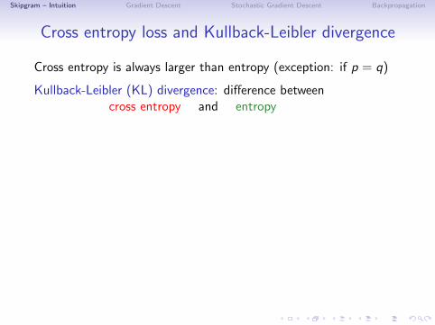
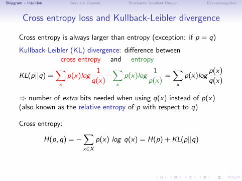
Cross entropy loss and Kullback-Leibler divergence
Cross entropy is always larger than entropy (exception: if p = q)
Kullback-Leibler (KL) divergence: difference betweencross entropy and entropy
KL(p||q) =∑x
p(x)log1
q(x)−∑x
p(x)log1
p(x)=∑x
p(x)logp(x)
q(x)
⇒ number of extra bits needed when using q(x) instead of p(x)(also known as the relative entropy of p with respect to q)
Cross entropy:
H(p, q) = −∑x∈X
p(x) log q(x) = H(p) + KL(p||q)
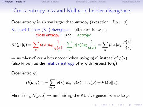
Minimising H(p, q) → minimising the KL divergence from q to p
Skipgram – Intuition Gradient Descent Stochastic Gradient Descent Backpropagation
Cross entropy loss and Kullback-Leibler divergence
Cross entropy is always larger than entropy (exception: if p = q)
Kullback-Leibler (KL) divergence: difference betweencross entropy and entropy
KL(p||q) =∑x
p(x)log1
q(x)−∑x
p(x)log1
p(x)=∑x
p(x)logp(x)
q(x)
⇒ number of extra bits needed when using q(x) instead of p(x)(also known as the relative entropy of p with respect to q)
Cross entropy:
H(p, q) = −∑x∈X
p(x) log q(x) = H(p) + KL(p||q)
Minimising H(p, q) → minimising the KL divergence from q to p
Skipgram – Intuition Gradient Descent Stochastic Gradient Descent Backpropagation
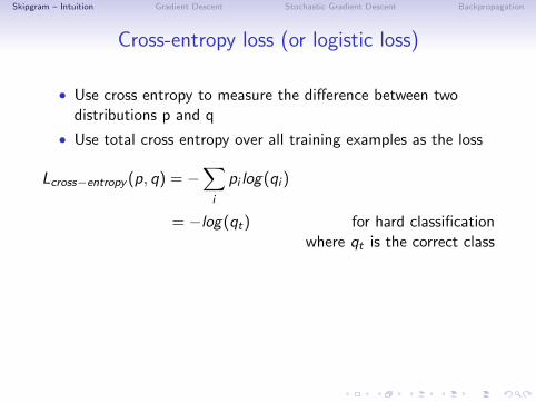
Cross-entropy loss (or logistic loss)
• Use cross entropy to measure the difference between twodistributions p and q
• Use total cross entropy over all training examples as the loss
Lcross−entropy (p, q) = −∑i
pi log(qi )
= −log(qt) for hard classificationwhere qt is the correct class
J(θ) = − 1T log L(θ) = − 1
T
T∑t=1
∑−m≤j≤m
log P(wt+j |wt ; θ)
j 6= 0
Negative log-likelihood = cross entropy

Skipgram – Intuition Gradient Descent Stochastic Gradient Descent Backpropagation
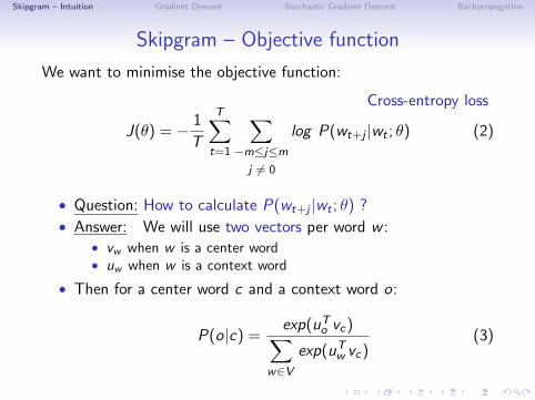
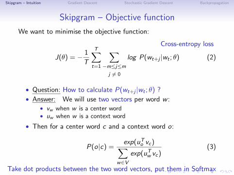
Skipgram – Objective function
We want to minimise the objective function:
Cross-entropy loss
J(θ) = − 1
T
T∑t=1
∑−m≤j≤m
log P(wt+j |wt ; θ) (2)
j 6= 0
• Question: How to calculate P(wt+j |wt ; θ) ?
• Answer: We will use two vectors per word w :• vw when w is a center word• uw when w is a context word
• Then for a center word c and a context word o:
P(o|c) =exp(uTo vc)∑
w∈Vexp(uTw vc)
(3)
Take dot products between the two word vectors, put them in Softmax
Skipgram – Intuition Gradient Descent Stochastic Gradient Descent Backpropagation
Skipgram – Objective function
We want to minimise the objective function:
Cross-entropy loss
J(θ) = − 1
T
T∑t=1
∑−m≤j≤m
log P(wt+j |wt ; θ) (2)
j 6= 0
• Question: How to calculate P(wt+j |wt ; θ) ?
• Answer: We will use two vectors per word w :• vw when w is a center word• uw when w is a context word
• Then for a center word c and a context word o:
P(o|c) =exp(uTo vc)∑
w∈Vexp(uTw vc)
(3)
Take dot products between the two word vectors, put them in Softmax

Skipgram – Intuition Gradient Descent Stochastic Gradient Descent Backpropagation
Recap: Dot products
• Measure of similarity (well, kind of...)
• Bigger if u and v are more similar(if vectors point in the same direction)
u>v = u · v =n∑
i=1
uivi (4)
• Iterating over w = 1 . . .W : u>w v
⇒ work out how similar each word is to v
P(o|c) =exp(uTo vc)
V∑w=1
exp(uTw vc)
(5)
Skipgram – Intuition Gradient Descent Stochastic Gradient Descent Backpropagation
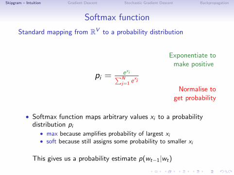
Softmax function
Standard mapping from RV to a probability distribution
Exponentiate tomake positive
pi = exi∑Nj=1 e
xj
Normalise toget probability
• Softmax function maps arbitrary values xi to a probabilitydistribution pi• max because amplifies probability of largest xi• soft because still assigns some probability to smaller xi
This gives us a probability estimate p(wt−1|wt)

Skipgram – Intuition Gradient Descent Stochastic Gradient Descent Backpropagation
Difference Sigmoid Function – Softmax
Sigmoid Function
• binary classification inlogistic regression
• sum of probabilities notnecessarily 1
• activation function
Softmax Function
• multi-classification inlogistic regression
• sum of probabilitieswill be 1

Skipgram – Intuition Gradient Descent Stochastic Gradient Descent Backpropagation
Why two representations for each word?
• We create two representations for each word in the corpus:
1. w as a context word2. w as a center word
• Easier to compute → we can optimise vectors separately
• Also works better in practice...
Skipgram – Intuition Gradient Descent Stochastic Gradient Descent Backpropagation
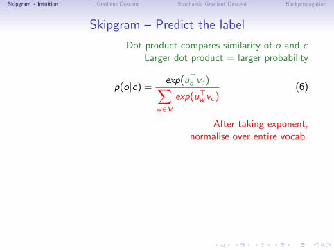
Skipgram – Predict the label
Dot product compares similarity of o and cLarger dot product = larger probability
p(o|c) =exp(u>o vc)∑
w∈Vexp(u>w vc)
(6)
After taking exponent,normalise over entire vocab
• For training the model, compute for all words in the corpus:
J(θ) = − 1T
T∑t=1
∑−m≤j≤m
log P(wt+j |wt ; θ)
j 6= 0

Skipgram – Intuition Gradient Descent Stochastic Gradient Descent Backpropagation
Skipgram – Training the model
• Recall: θ represents all model parameters, in one long vector
• For d-dimensional vectors and V-many words:
θ =
vaasvamaranth...vzoouaasuameise...uzoo
∈ R2dV (7)
• Remember: every word has two vectors ⇒ 2d
• We now optimise the parameters θ
Skipgram – Intuition Gradient Descent Stochastic Gradient Descent Backpropagation
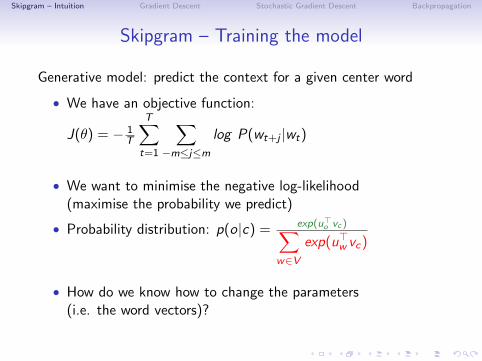
Skipgram – Training the model
Generative model: predict the context for a given center word
• We have an objective function:
J(θ) = − 1T
T∑t=1
∑−m≤j≤m
log P(wt+j |wt)
• We want to minimise the negative log-likelihood(maximise the probability we predict)
• Probability distribution: p(o|c) = exp(u>o vc )∑w∈V
exp(u>w vc)
• How do we know how to change the parameters(i.e. the word vectors)?
→ Use the gradient
Skipgram – Intuition Gradient Descent Stochastic Gradient Descent Backpropagation
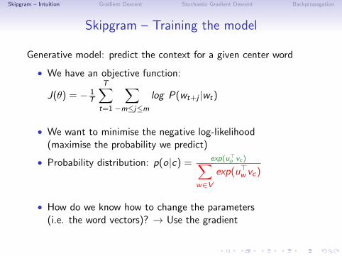
Skipgram – Training the model
Generative model: predict the context for a given center word
• We have an objective function:
J(θ) = − 1T
T∑t=1
∑−m≤j≤m
log P(wt+j |wt)
• We want to minimise the negative log-likelihood(maximise the probability we predict)
• Probability distribution: p(o|c) = exp(u>o vc )∑w∈V
exp(u>w vc)
• How do we know how to change the parameters(i.e. the word vectors)? → Use the gradient
Skipgram – Intuition Gradient Descent Stochastic Gradient Descent Backpropagation
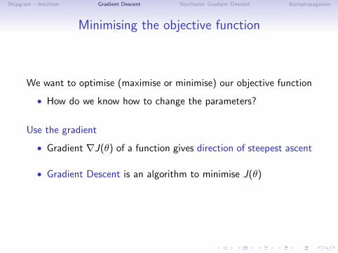
Minimising the objective function
We want to optimise (maximise or minimise) our objective function
• How do we know how to change the parameters?
Use the gradient
• Gradient ∇J(θ) of a function gives direction of steepest ascent
• Gradient Descent is an algorithm to minimise J(θ)
Skipgram – Intuition Gradient Descent Stochastic Gradient Descent Backpropagation
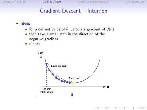
Gradient Descent – Intuition
• Idea:• for a current value of θ, calculate gradient of J(θ)• then take a small step in the direction of the
negative gradient• repeat

Skipgram – Intuition Gradient Descent Stochastic Gradient Descent Backpropagation
Gradient Descent – Intuition
• Find local minimum for a given cost function• at each step, GD tells us in which direction to move
to lower the cost
• No guarantee that we find the best global solution!
Skipgram – Intuition Gradient Descent Stochastic Gradient Descent Backpropagation
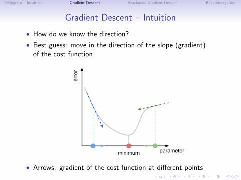
Gradient Descent – Intuition
• How do we know the direction?
• Best guess: move in the direction of the slope (gradient)of the cost function
• Arrows: gradient of the cost function at different points
Skipgram – Intuition Gradient Descent Stochastic Gradient Descent Backpropagation
Gradient Descent – Intuition
• Gradient of a function• vector that points in the direction of the steepest ascent
• Gradient is deeply connected to its derivative
• Derivative f ′ of a function• a single number that indicates how fast the function is rising
when moving in the direction of its gradient
• f ′(p): value of f ′ at point p• f ′(p) > 0⇒ f is going up• f ′(p) < 0⇒ f is going down• f ′(p) = 0⇒ f is flat

Skipgram – Intuition Gradient Descent Stochastic Gradient Descent Backpropagation
Gradient-Based OptimisationGiven some function y = f (x) with x , y ∈ R
• We want to optimise (maximise or minimise) it by updating x
minx∈Rf (x)
• Gradient Descent: reduce f (x) by moving x in small stepswith the opposite sign of the derivative
What if we have functions with multiple inputs?

Skipgram – Intuition Gradient Descent Stochastic Gradient Descent Backpropagation
Gradient-Based OptimisationGiven some function y = f (x) with x , y ∈ R
• minx∈Rf (x)
• Gradient Descent: reduce f (x) by moving x in small stepswith the opposite sign of the derivative
What if we have functions with multiple inputs?

Skipgram – Intuition Gradient Descent Stochastic Gradient Descent Backpropagation
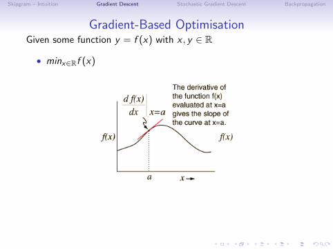
Gradient-Based Optimisation
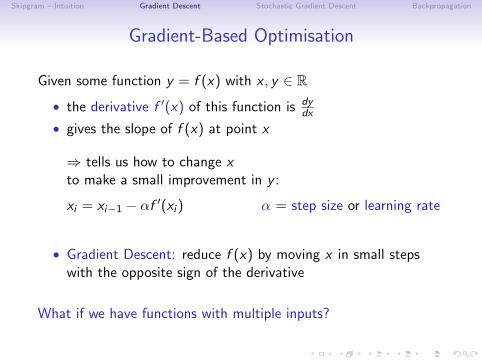
Given some function y = f (x) with x , y ∈ R
• the derivative f ′(x) of this function is dydx
• gives the slope of f (x) at point x
⇒ tells us how to change xto make a small improvement in y :
xi = xi−1 − αf ′(xi ) α = step size or learning rate
• Gradient Descent: reduce f (x) by moving x in small stepswith the opposite sign of the derivative
What if we have functions with multiple inputs?

Skipgram – Intuition Gradient Descent Stochastic Gradient Descent Backpropagation
Gradient-Based Optimisation
Given some function y = f (x) with x , y ∈ R
• the derivative f ′(x) of this function is dydx
• gives the slope of f (x) at point x
⇒ tells us how to change xto make a small improvement in y :
xi = xi−1 − αf ′(xi ) α = step size or learning rate
• Gradient Descent: reduce f (x) by moving x in small stepswith the opposite sign of the derivative
What if we have functions with multiple inputs?
Skipgram – Intuition Gradient Descent Stochastic Gradient Descent Backpropagation
Gradient Descent with multiple inputs
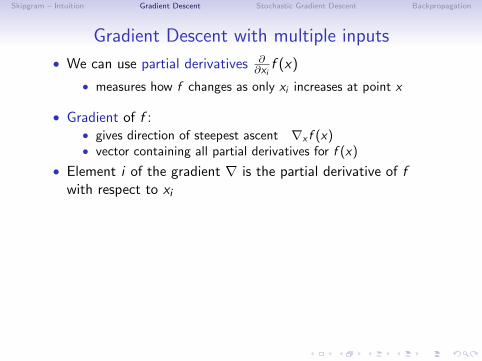
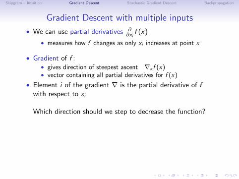
• We can use partial derivatives ∂∂xi
f (x)
• measures how f changes as only xi increases at point x
• Gradient of f :• gives direction of steepest ascent ∇x f (x)• vector containing all partial derivatives for f (x)
• Element i of the gradient ∇ is the partial derivative of fwith respect to xi
Which direction should we step to decrease the function?
• Gradient descent algorithm:
• compute ∇x f (x)• take small step in −∇x f (x) direction• repeat
• Minimise f by applying small updates to x : x ′ = x −α∇x f (x)
Skipgram – Intuition Gradient Descent Stochastic Gradient Descent Backpropagation
Gradient Descent with multiple inputs
• We can use partial derivatives ∂∂xi
f (x)
• measures how f changes as only xi increases at point x
• Gradient of f :• gives direction of steepest ascent ∇x f (x)• vector containing all partial derivatives for f (x)
• Element i of the gradient ∇ is the partial derivative of fwith respect to xi
Which direction should we step to decrease the function?
• Gradient descent algorithm:
• compute ∇x f (x)• take small step in −∇x f (x) direction• repeat
• Minimise f by applying small updates to x : x ′ = x −α∇x f (x)

Skipgram – Intuition Gradient Descent Stochastic Gradient Descent Backpropagation
Gradient Descent with multiple inputs
Critical points in 2D (one input value):
Skipgram – Intuition Gradient Descent Stochastic Gradient Descent Backpropagation
Gradient Descent with multiple inputs
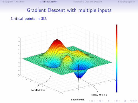
Critical points in 3D:
Skipgram – Intuition Gradient Descent Stochastic Gradient Descent Backpropagation
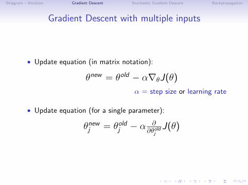
Gradient Descent with multiple inputs
• Update equation (in matrix notation):
θnew = θold − α∇θJ(θ)
α = step size or learning rate
• Update equation (for a single parameter):
θnewj = θoldj − α ∂∂θoldj
J(θ)
Skipgram – Intuition Gradient Descent Stochastic Gradient Descent Backpropagation
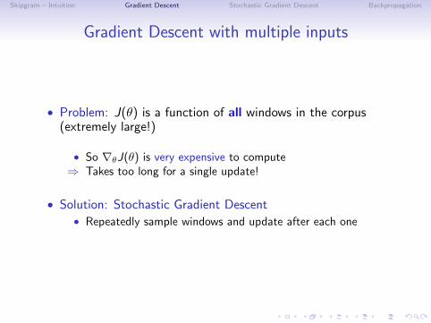
Gradient Descent with multiple inputs
• Problem: J(θ) is a function of all windows in the corpus(extremely large!)
• So ∇θJ(θ) is very expensive to compute⇒ Takes too long for a single update!
• Solution: Stochastic Gradient Descent• Repeatedly sample windows and update after each one
Skipgram – Intuition Gradient Descent Stochastic Gradient Descent Backpropagation
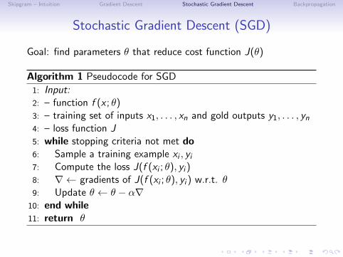
Stochastic Gradient Descent (SGD)
Goal: find parameters θ that reduce cost function J(θ)
Algorithm 1 Pseudocode for SGD
1: Input:2: – function f (x ; θ)3: – training set of inputs x1, . . . , xn and gold outputs y1, . . . , yn4: – loss function J5: while stopping criteria not met do6: Sample a training example xi , yi7: Compute the loss J(f (xi ; θ), yi )8: ∇ ← gradients of J(f (xi ; θ), yi ) w.r.t. θ9: Update θ ← θ − α∇
10: end while11: return θ
Skipgram – Intuition Gradient Descent Stochastic Gradient Descent Backpropagation
Stochastic Gradient Descent (SGD)
Goal: find parameters θ that reduce cost function J(θ)
• Impact of learning rate α:• too low → learning proceeds slowly• initial α too low → learning may become stuck with high cost

Skipgram – Intuition Gradient Descent Stochastic Gradient Descent Backpropagation
Stochastic Gradient Descent (SGD)
Goal: find parameters θ that reduce cost function J(θ)
• Important property of SGD (and related minibatch or onlinegradient-based optimization)• computation time per update does not grow with increasing
number of training examples

Skipgram – Intuition Gradient Descent Stochastic Gradient Descent Backpropagation
Stochastic Gradient Descent (SGD)
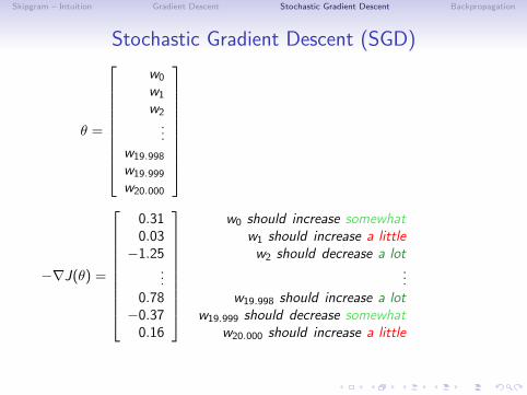
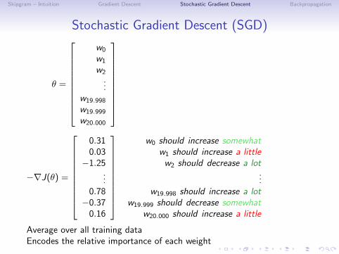
θ =
w0
w1
w2
...w19.998
w19.999
w20.000
−∇J(θ) =
0.310.03−1.25
...0.78−0.37
0.16
w0 should increase somewhatw1 should increase a littlew2 should decrease a lot
...w19.998 should increase a lot
w19.999 should decrease somewhatw20.000 should increase a little

Skipgram – Intuition Gradient Descent Stochastic Gradient Descent Backpropagation
Stochastic Gradient Descent (SGD)
θ =
w0
w1
w2
...w19.998
w19.999
w20.000
−∇J(θ) =
0.310.03−1.25
...0.78−0.37
0.16
w0 should increase somewhatw1 should increase a littlew2 should decrease a lot
...w19.998 should increase a lot
w19.999 should decrease somewhatw20.000 should increase a little
Average over all training dataEncodes the relative importance of each weight

Skipgram – Intuition Gradient Descent Stochastic Gradient Descent Backpropagation
Stochastic Gradient Descent (SGD)
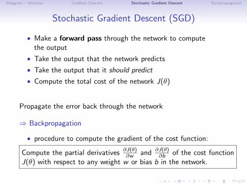
• Make a forward pass through the network to computethe output
• Take the output that the network predicts
• Take the output that it should predict
• Compute the total cost of the network J(θ)
Propagate the error back through the network
⇒ Backpropagation
• procedure to compute the gradient of the cost function:
Skipgram – Intuition Gradient Descent Stochastic Gradient Descent Backpropagation
Stochastic Gradient Descent (SGD)
• Make a forward pass through the network to computethe output
• Take the output that the network predicts
• Take the output that it should predict
• Compute the total cost of the network J(θ)
Propagate the error back through the network
⇒ Backpropagation
• procedure to compute the gradient of the cost function:
Compute the partial derivatives ∂J(θ)∂w and ∂J(θ)
∂b of the cost functionJ(θ) with respect to any weight w or bias b in the network.

Skipgram – Intuition Gradient Descent Stochastic Gradient Descent Backpropagation
Stochastic Gradient Descent (SGD)
• Make a forward pass through the network to computethe output
• Take the output that the network predicts
• Take the output that it should predict
• Compute the total cost of the network J(θ)
Propagate the error back through the network
⇒ Backpropagation
• procedure to compute the gradient of the cost function:
How do we have to change the weights and biasesin order to change the cost?

Skipgram – Intuition Gradient Descent Stochastic Gradient Descent Backpropagation
Parameter initialisation
• Before we start training the network we have to initialise theparameters• Why not use zero as initial values?• Not a good idea, outputs will be the same for all nodes• Instead, use small random numbers, e.g.:
• use normally distributed values around zero N(0, 0.1)• use Xavier initialisation (Glorot and Bengio 2010)• for debugging: use fixed random seeds
• Now let’s start the training:• predict labels• compute loss• update parameters
Skipgram – Intuition Gradient Descent Stochastic Gradient Descent Backpropagation
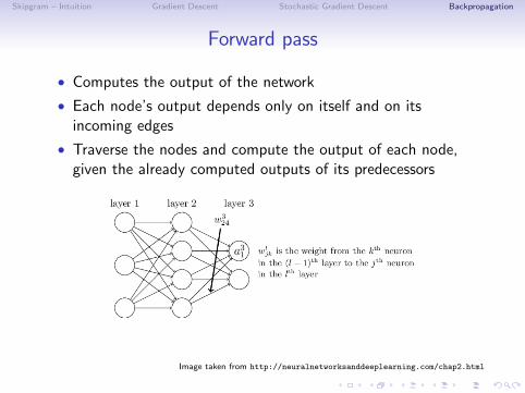
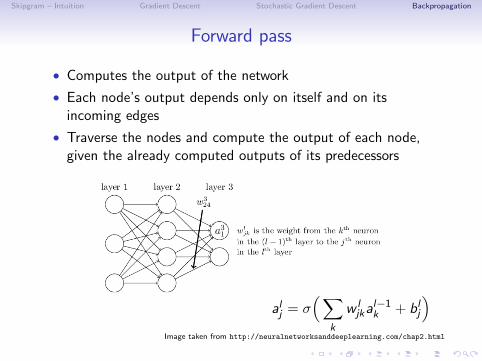
Forward pass
• Computes the output of the network
• Each node’s output depends only on itself and on itsincoming edges
• Traverse the nodes and compute the output of each node,given the already computed outputs of its predecessors
Image taken from http://neuralnetworksanddeeplearning.com/chap2.html
Skipgram – Intuition Gradient Descent Stochastic Gradient Descent Backpropagation
Forward pass
• Computes the output of the network
• Each node’s output depends only on itself and on itsincoming edges
• Traverse the nodes and compute the output of each node,given the already computed outputs of its predecessors
alj = σ(∑
k
w ljka
l−1k + blj
)Image taken from http://neuralnetworksanddeeplearning.com/chap2.html

Skipgram – Intuition Gradient Descent Stochastic Gradient Descent Backpropagation
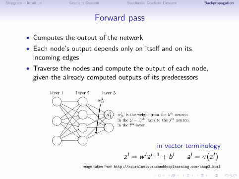
Forward pass
• Computes the output of the network
• Each node’s output depends only on itself and on itsincoming edges
• Traverse the nodes and compute the output of each node,given the already computed outputs of its predecessors
in vector terminology
al = σ(w lal−1 + bl
)Image taken from http://neuralnetworksanddeeplearning.com/chap2.html
Skipgram – Intuition Gradient Descent Stochastic Gradient Descent Backpropagation
Forward pass
• Computes the output of the network
• Each node’s output depends only on itself and on itsincoming edges
• Traverse the nodes and compute the output of each node,given the already computed outputs of its predecessors
in vector terminology
z l = w lal−1 + bl al = σ(z l)Image taken from http://neuralnetworksanddeeplearning.com/chap2.html

Skipgram – Intuition Gradient Descent Stochastic Gradient Descent Backpropagation
Parameter update for a 1-layer network
• After a single forward pass, predict the output y
• Compute the cost J (a single scalar value), given thepredicted y and the ground truth y
• Take the derivative of the cost J w.r.t w and b
• Update w and b by a fraction (learning rate) of dw and db

Skipgram – Intuition Gradient Descent Stochastic Gradient Descent Backpropagation
Parameter update for a 1-layer network
Forward pass:
Z = W>X + by = A = σ(Z )
Use the chain rule:
dJdW = dJ
dAdAdZ
dZdW
dJdb = dJ
dAdAdZ
dZdb
Update w and b:
W = W − α dJdW
b = b − αdJdb
Image taken from http://www.adeveloperdiary.com/data-science/machine-learning/
understand-and-implement-the-backpropagation-algorithm-from-scratch-in-python/
Skipgram – Intuition Gradient Descent Stochastic Gradient Descent Backpropagation
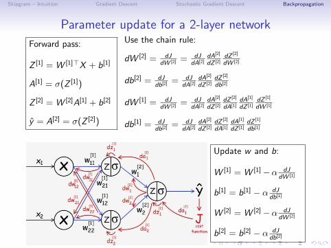
Parameter update for a 2-layer network
Forward pass:
Z [1] = W [1]>X + b[1]
A[1] = σ(Z [1])
Z [2] = W [2]A[1] + b[2]
y = A[2] = σ(Z [2])
Use the chain rule:
dW [2] = dJdW [2] = dJ
dA[2]dA[2]
dZ [2]dZ [2]
dW [2]
db[2] = dJdb[2] = dJ
dA[2]dA[2]
dZ [2]dZ [2]
db[2]
dW [1] = dJdW [2] = dJ
dA[2]dA[2]
dZ [2]dZ [2]
dA[1]dA[1]
dZ [1]dZ [1]
dW [1]
db[1] = dJdb[2] = dJ
dA[2]dA[2]
dZ [2]dZ [2]
dA[1]dA[1]
dZ [1]dZ [1]
db[1]
Update w and b:
W [1] = W [1]−α dJdW [1]
b[1] = b[1] − α dJdb[1]
W [2] = W [2]−α dJdW [2]
b[2] = b[2] − α dJdb[2]

Skipgram – Intuition Gradient Descent Stochastic Gradient Descent Backpropagation
Training with SGD and backpropagation
• Randomly initialise parameters w and b
• For iteration 1 .. N; do• predict y based on w , b and x• compute the loss (or cost) J• find dJ
dW and dJdb
• update w and b using dw and db
With increasing number of layers in the network:computation complexity increases exponentially
⇒ use dynamic programming
Skipgram – Intuition Gradient Descent Stochastic Gradient Descent Backpropagation
Training with SGD and backpropagation
• Backpropagation:• efficient method for computing gradients in a directed
computation graph (e.g. a NN)• implementation of chain rule of derivatives,• allows us to compute all required partial derivatives in linear
time in terms of the graph size
• Stochastic Gradient Descent• optimisation method, based on the analysis of the gradient of
the objective function
• Backpropagation is often used in combination with SGD
Gradient computation: backpropOptimisation: SGD, Adam, Rprop, BFGS, ...

Skipgram – Intuition Gradient Descent Stochastic Gradient Descent Backpropagation
Lecture slide from C. Manning, Stanford University (CS224n, Lecture 2)
Skipgram – Intuition Gradient Descent Stochastic Gradient Descent Backpropagation
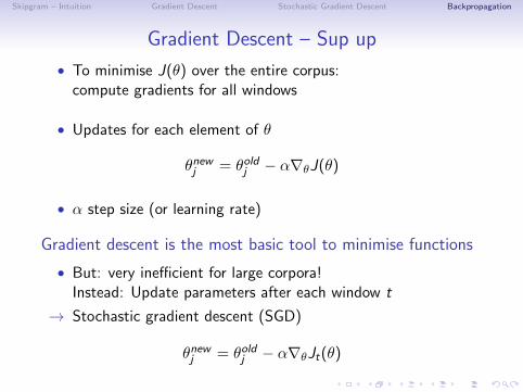
Gradient Descent – Sup up
• To minimise J(θ) over the entire corpus:compute gradients for all windows
• Updates for each element of θ
θnewj = θoldj − α∇θJ(θ)
• α step size (or learning rate)
Gradient descent is the most basic tool to minimise functions
• But: very inefficient for large corpora!Instead: Update parameters after each window t
→ Stochastic gradient descent (SGD)
θnewj = θoldj − α∇θJt(θ)

Skipgram – Intuition Gradient Descent Stochastic Gradient Descent Backpropagation
Skipgram in a nutshell
• Train a simple neural network with a single hidden layer
• Throw away the network, only keep the learned weights of thehidden layer ⇒ word embeddings
• Limitations of the model• Normalisation factor is computationally expensive
p(o|c) =exp(u>
o vc )
V∑w=1
exp(u>w vc)
• Solution: Skipgram with negative sampling(randomly sample “negative” instances from the copurs)


![Deep Learning Framework based on Word2Vec and CNN for ... · space [4]. Moreover, with Word2vec features can be obtained without human intervention. Word2Vec can also perform effectively](https://static.fdocuments.in/doc/165x107/5f0a677f7e708231d42b781f/deep-learning-framework-based-on-word2vec-and-cnn-for-space-4-moreover-with.jpg)


![Comparative study of LSA vs Word2vec embeddings … · Comparative study of LSA vs Word2vec embeddings in small corpora: ... 1 Introduction ... ,psychology[4,5],philology[6],cognitivescience[7]andsocial](https://static.fdocuments.in/doc/165x107/5b819a897f8b9ae87c8ca81e/comparative-study-of-lsa-vs-word2vec-embeddings-comparative-study-of-lsa-vs.jpg)

![Word Embeddingssvivek.com/.../spring2019/slides/word-embeddings/4-word2vec-glove… · enough [Mikolov, 2013, word2vec] –Simpler model, fewer parameters –Faster to train 4 Context](https://static.fdocuments.in/doc/165x107/5f0a677c7e708231d42b7810/word-enough-mikolov-2013-word2vec-asimpler-model-fewer-parameters-afaster.jpg)