Word embeddings (II)

CS 490A, Fall 2021https://people.cs.umass.edu/~brenocon/cs490a_f21/

Laure Thompson and Brendan O'Connor

College of Information and Computer SciencesUniversity of Massachusetts Amherst

Announcements• HW3 extension • Project proposal feedback

• Schedule your TA meeting! 20 minutes, all members and TA, to discuss your project. • TA emails should be out now. Please email them if you don't see -

your TA is in the feedback blurb. • Please schedule tonight/tomorrow.

"Exercise 9: schedule meeting"; only TAs can mark you as done. • Project proposal revision option, to get 100 points • Next week

• We have a little take-home exercise to explore word embeddings • Midterm review questions • Tuesday: neural network models for NLP • Thursday: midterm review session - come with questions on

anything!

2

• Distributional semantics: • a word's meaning is related to how it's used • we approximate that from its context distribution in a corpus • word embeddings: we can reduce this dimensionality into,

say, 100 latent dimensions of meaning (matrix factorization: LSA or SGNS)

• Today: So what do you get from word embeddings / distributional info? • Lookup similar words (with what function?) • Automatically cluster words by syntax?/topic?/meaning? • "Bag of embeddings" model for text classification • Exploratory analysis of both docs and words

3

Word embeddings pipeline

• Word embeddings are a lexical resource, to be used for downstream tasks • Transfer learning: get info huge corpus, then apply to learn from a small labeled dataset

• Compare to lexicons, lexical knowledge bases like WordNet, etc.4

Pre-trained embeddings

• Demo!

• Widely useful. But make sure you know what you’re getting!

• Examples: GLOVE, fasttext, word2vec, etc. • Is the corpus similar to what you care about? • Should you care about the data?

5

Alternate/mis- spellings

• Distributional methods are really good at this • Twitter-trained word clusters:

http://www.cs.cmu.edu/~ark/TweetNLP/cluster_viewer.html

• See also: GLOVE website has Twitter-trained word embeddings

6

Evaluating embeddings• Intrinsic evaluations

• Compare embeddings’ word pair similarities to human judgments

• TOEFL: “Levied is closest to imposed, believed, requested, correlated”

• Numerical similarity judgments (e.g. Wordsim-353) • Attempt to look at structure of the embedding

space, such as analogies • Controversial; see Linzen 2016

• Extrinsic evaluation: use embeddings in some task

7

8

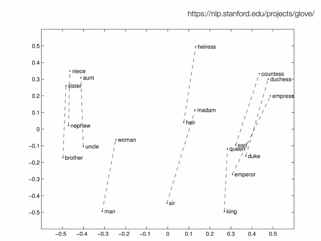
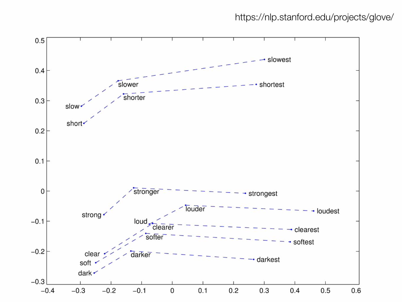
https://nlp.stanford.edu/projects/glove/

9

https://nlp.stanford.edu/projects/glove/

Application: keyword expansion

• Other non-embedding lexical resources can do this too (e.g. WordNet), but word embeddings typically cover a lot of diverse vocabulary

10

• I have a few keywords for my task. Are there any I missed? • Automated or semi-automated new terms from embedding neighbors

Application: document embedding• Instead of bag-of-words, can we derive a latent

embedding of a document/sentence?

11 See: Arora et al. 2017

Transfer learning

• Sparsity problems for traditional bag-of-words

• Labeled datasets are small … but unlabeled data is much bigger!

12

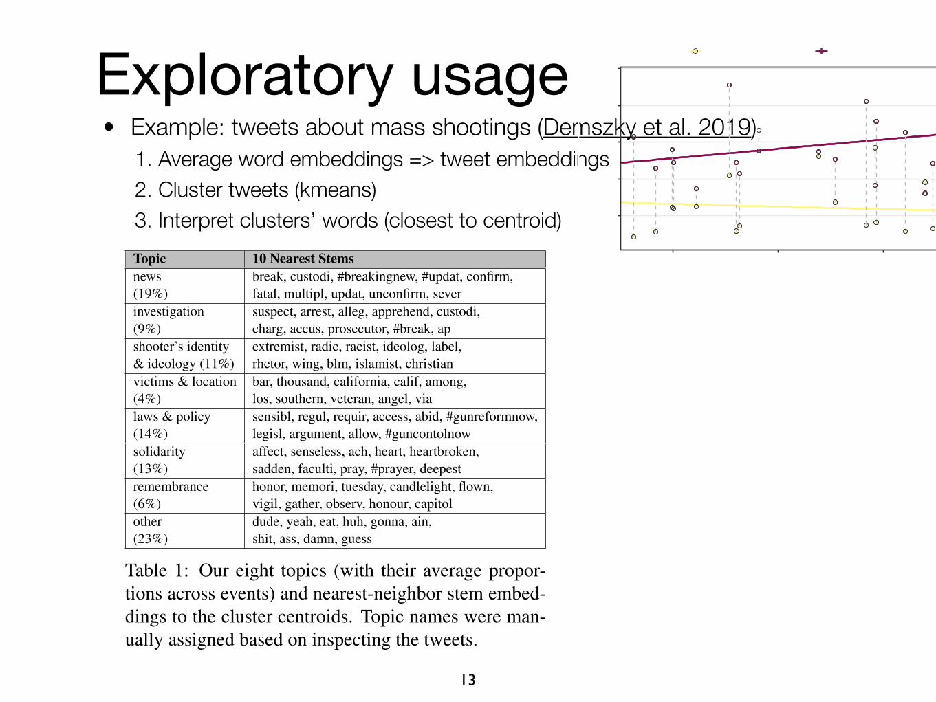
Exploratory usage• Example: tweets about mass shootings (Demszky et al. 2019)

1. Average word embeddings => tweet embeddings 2. Cluster tweets (kmeans) 3. Interpret clusters’ words (closest to centroid)

13

2974

Figure 4: Topic model evaluations, collapsed acrossk = 6� 10. Error bars denote standard errors.

Topic 10 Nearest Stemsnews(19%)

break, custodi, #breakingnew, #updat, confirm,fatal, multipl, updat, unconfirm, sever

investigation(9%)

suspect, arrest, alleg, apprehend, custodi,charg, accus, prosecutor, #break, ap

shooter’s identity& ideology (11%)

extremist, radic, racist, ideolog, label,rhetor, wing, blm, islamist, christian

victims & location(4%)

bar, thousand, california, calif, among,los, southern, veteran, angel, via

laws & policy(14%)

sensibl, regul, requir, access, abid, #gunreformnow,legisl, argument, allow, #guncontolnow

solidarity(13%)

affect, senseless, ach, heart, heartbroken,sadden, faculti, pray, #prayer, deepest

remembrance(6%)

honor, memori, tuesday, candlelight, flown,vigil, gather, observ, honour, capitol

other(23%)

dude, yeah, eat, huh, gonna, ain,shit, ass, damn, guess

Table 1: Our eight topics (with their average propor-tions across events) and nearest-neighbor stem embed-dings to the cluster centroids. Topic names were man-ually assigned based on inspecting the tweets.

To compare the models, we ran two MTurk ex-periments: a word intrusion task (Chang et al.,2009) and our own, analogically defined tweet in-trusion task, with the number of topics k rangingbetween 6-10. Turkers were presented with eithera set of 6 words (for word intrusion) or a set of4 tweets (for tweet intrusion), all except one ofwhich was close (in terms of d) to a randomly cho-sen topic and one that was far from that topic butclose to another topic. Then, Turkers were askedto pick the odd one out among the set of words /tweets. More details in Appendix D.

We find that our model outperforms the LDA-based methods with respect to both tasks, particu-larly tweet intrusion — see Figure 4. This suggeststhat our model both provides more cohesive topicsat the word level and more cohesive groupings bytopic assignment. The choice of k does not yielda significant difference among model-level accu-racies. However, since k = 8 slightly outperformsother k-s in tweet intrusion, we use it for furtheranalysis. See Table 1 for nearest neighbor stems toeach topic and Appendix C.2 for example tweets.

Measuring within-topic and between-topic par-tisanship. Recall that the leave-out estimator

SD=4%) across events, for our model, for eight topics.

AnnapolisBaton Rouge

BurlingtonChattanooga

Colorado SpringsDallas

Fresno

Kalamazoo Nashville

Orlando

Parkland

Pittsburgh

Roseburg

San BernardinoSan Francisco

Santa Fe

Sutherland Springs

Thornton

Thousand OaksVegas

0.51

0.52

0.53

0.54

0.55

2016 2017 2018 2019Year

Pola

rizat

ion

between−topic within−topic

Figure 5: Measurements of between-topic and within-topic polarization of the 21 events in our dataset showthat within-topic polarization is increasing over timewhile between-topic polarization remains stable.

from Section 3.1 provides a measure of partisan-ship. The information in a tweet, and thus par-tisanship, can be decomposed into which topic isdiscussed, and how it’s discussed.

To measure within-topic partisanship for a par-ticular event, i.e. how a user discusses a giventopic, we re-apply the leave-out estimator. Foreach topic, we calculate the partisanship usingonly tweets categorized to that topic. Then, over-all within-topic partisanship for the event is theweighted mean of these values, with weights givenby the proportion of tweets categorized to eachtopic within each event.

Between-topic partisanship is defined as the ex-pected posterior that an observer with a neutralprior would assign to a user’s true party after learn-ing only the topic — but not the words — of auser’s tweet. We estimate this value by replacingeach tweet with its assigned topic and applying theleave-out estimator to this data.

4.2 Results

Figure 5 shows that for most events within-topic ishigher than between-topic partisanship, suggest-ing that while topic choice does play a role inphrase partisanship (its values are meaningfullyhigher than .5), within-topic phrase usage is sig-nificantly more polarized. Linear estimates ofthe relationship between within and between topicpartisanship and time show that while within-topicpolarization has increased over time, between-topic polarization has remained stable. This find-ing supports the idea that topic choice and topic-level framing are distinct phenomena.

Partisanship also differs by topic, and withindays after a given event. Figure 6 shows po-larization within topics for 9 days after Las Ve-

14

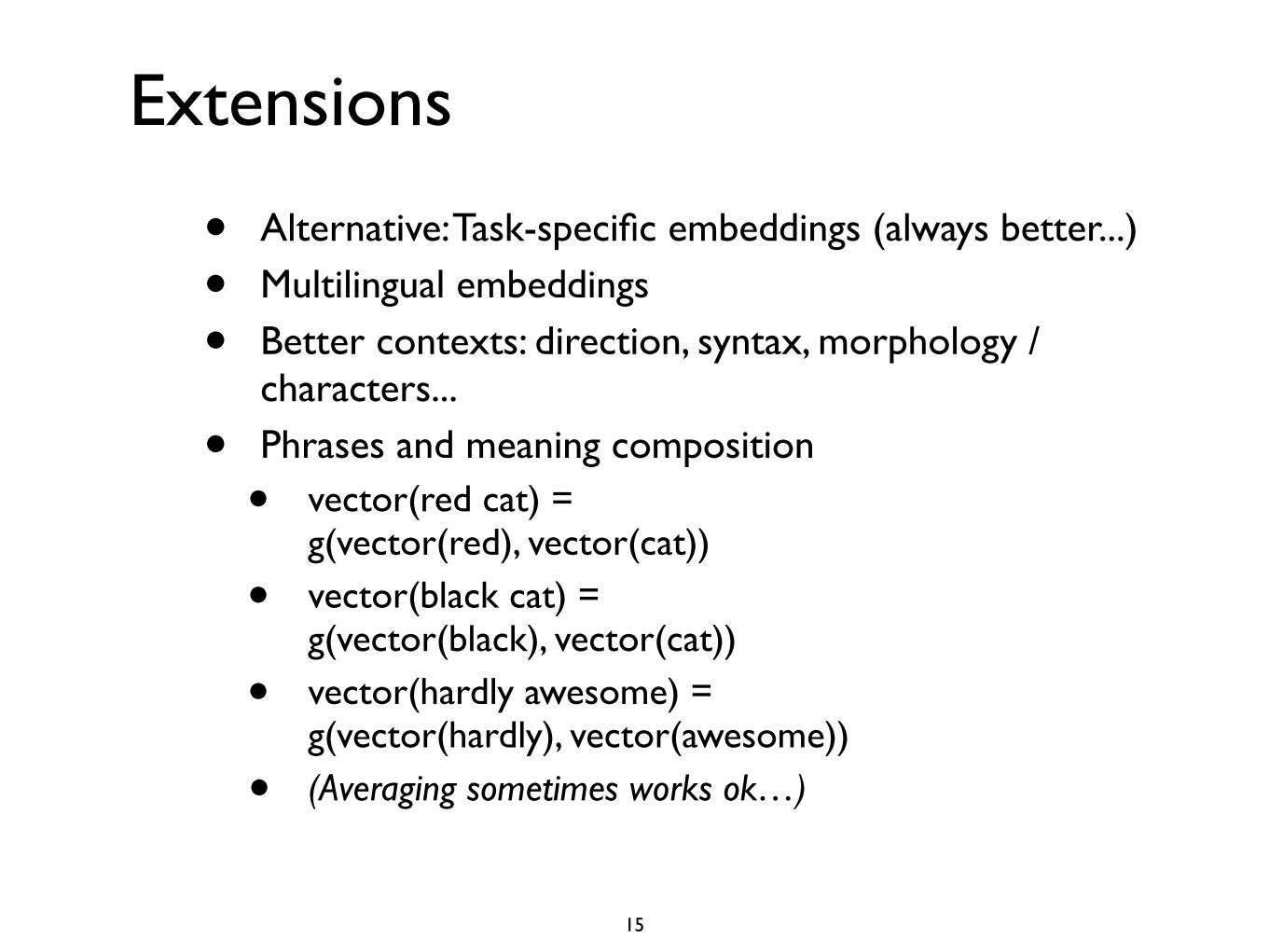
Extensions

• Alternative: Task-specific embeddings (always better...)

• Multilingual embeddings

• Better contexts: direction, syntax, morphology / characters...

• Phrases and meaning composition

• vector(red cat) = g(vector(red), vector(cat))

• vector(black cat) = g(vector(black), vector(cat))

• vector(hardly awesome) = g(vector(hardly), vector(awesome))

• (Averaging sometimes works ok…)

15

16

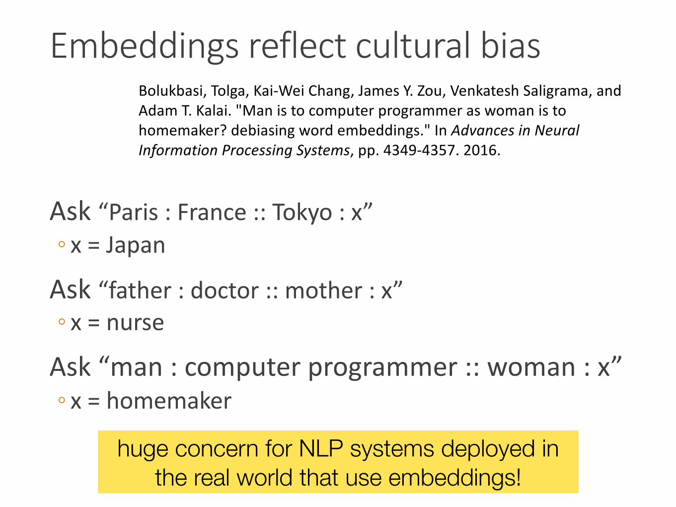
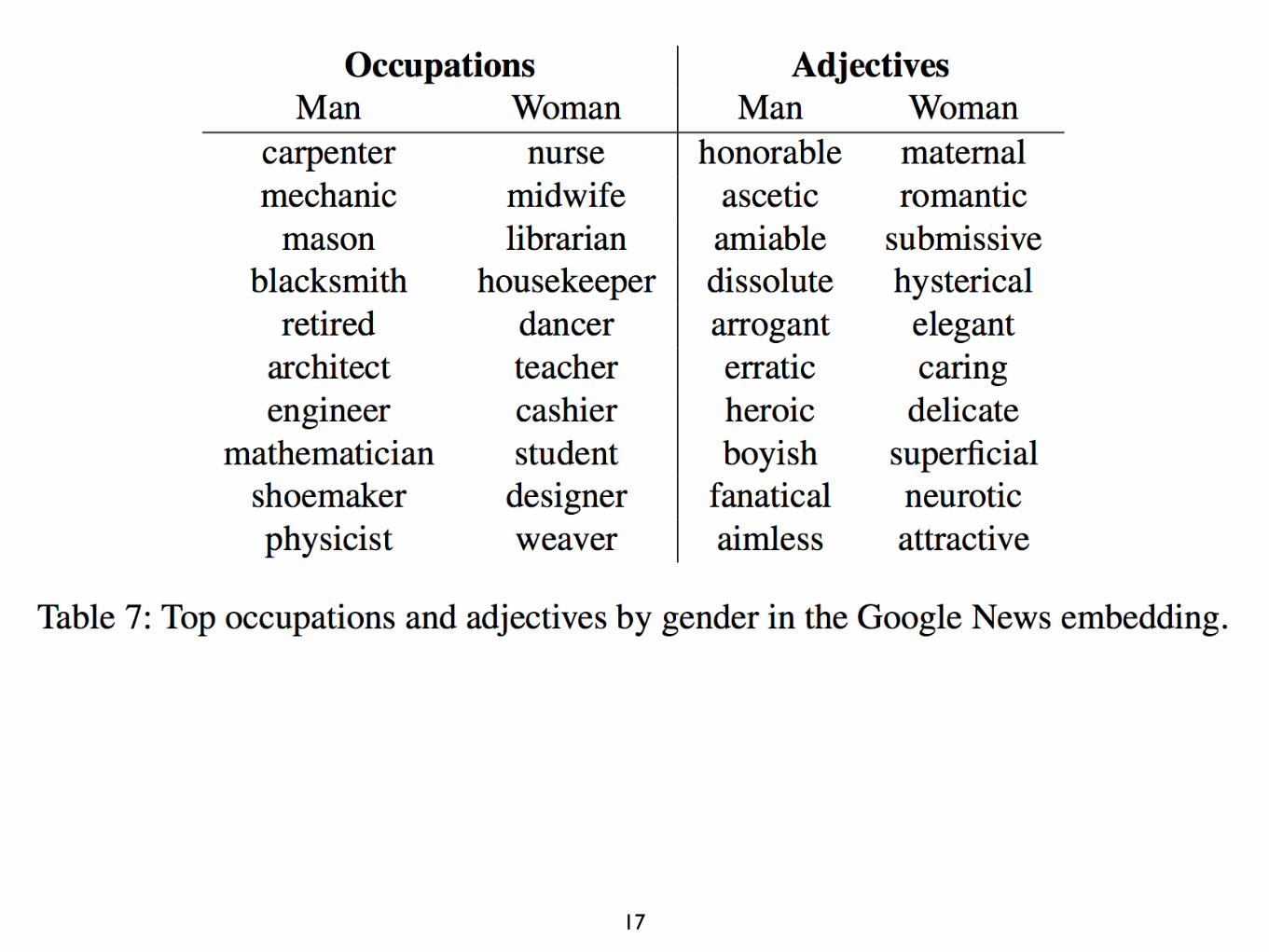
Embeddings reflect cultural bias

Ask “Paris : France :: Tokyo : x” ◦ x = Japan

Ask “father : doctor :: mother : x” ◦ x = nurse

Ask “man : computer programmer :: woman : x” ◦ x = homemaker

Bolukbasi, Tolga, Kai-Wei Chang, James Y. Zou, Venkatesh Saligrama, and Adam T. Kalai. "Man is to computer programmer as woman is to homemaker? debiasing word embeddings." In Advances in Neural Information Processing Systems, pp. 4349-4357. 2016.

huge concern for NLP systems deployed in the real world that use embeddings!

17

18

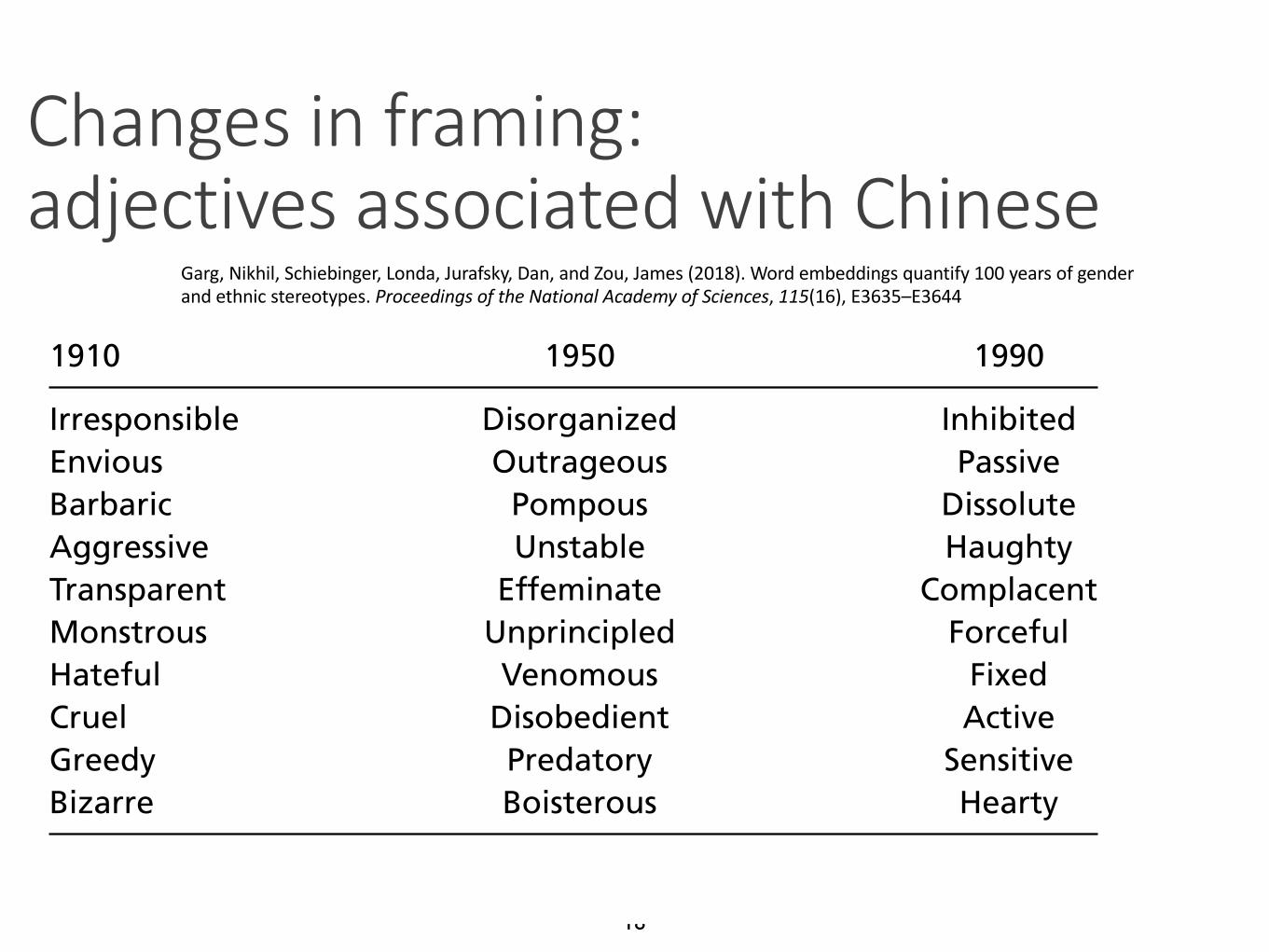
Changes in framing:adjectives associated with Chinese

CO

MP

UTER

SC

IEN

CES

SO

CIA

LS

CIE

NC

ES

Table 3. Top Asian (vs. White) adjectives in 1910, 1950, and 1990by relative norm difference in the COHA embedding

1910 1950 1990

Irresponsible Disorganized InhibitedEnvious Outrageous PassiveBarbaric Pompous DissoluteAggressive Unstable HaughtyTransparent Effeminate ComplacentMonstrous Unprincipled ForcefulHateful Venomous FixedCruel Disobedient ActiveGreedy Predatory SensitiveBizarre Boisterous Hearty

qualitatively through the results in the snapshot analysis for gen-der, which replicates prior work, and quantitatively as the metricscorrelate highly with one another, as shown in SI Appendix,section A.5.

Furthermore, we primarily use linear models to fit the relation-ship between embedding bias and various external metrics; how-ever, the true relationships may be nonlinear and warrant furtherstudy. This concern is especially salient when studying ethnicstereotypes over time in the United States, as immigration dras-tically shifts the size of each group as a percentage of the popu-lation, which may interact with stereotypes and occupation per-centages. However, the models are sufficient to show consistencyin the relationships between embedding bias and external metricsacross datasets over time. Further, the results do not qualitativelychange when, for example, population logit proportion insteadof raw percentage difference is used, as in ref. 44; we reproduceour primary figures with such a transformation in SI Appendix,section A.6.

Another potential concern may be the dependency of ourresults on the specific word lists used and that the recall ofour methods in capturing human biases may not be adequate.We take extensive care to reproduce similar results with otherword lists and types of measurements to demonstrate recall. Forexample, in SI Appendix, section B.1, we repeat the static occu-pation analysis using only professional occupations and repro-duce an identical figure to Fig. 1 in SI Appendix, section B.1.Furthermore, the plots themselves contain bootstrapped confi-dence intervals; i.e., the coefficients for random subsets of theoccupations/adjectives and the intervals are tight. Similarly, foradjectives, we use two different lists: one list from refs. 6 and 7for which we have labeled stereotype scores and then a largerone for the rest of the analysis where such scores are not needed.We note that we do not tune either the embeddings or the wordlists, instead opting for the largest/most general publicly avail-able data. For reproducibility, we share our code and all wordlists in a repository. That our methods replicate across many dif-ferent embeddings and types of biases measured suggests theirgeneralizability.

A common challenge in historical analysis is that the writtentext in, say 1910, may not completely reflect the popular socialattitude of that time. This is an important caveat to consider ininterpreting the results of the embeddings trained on these ear-lier text corpora. The fact that the embedding bias for genderand ethnic groups does track with census proportion is a positivecontrol that the embedding is still capturing meaningful patternsdespite possible limitations in the training text. Even this con-trol may be limited in that the census proportion does not fullycapture gender or ethnic associations, even in the present day.However, the written text does serve as a window into the atti-tudes of the day as expressed in popular culture, and this workallows for a more systematic study of such text.

Another limitation of our current approach is that all of theembeddings used are fully “black box,” where the dimensionshave no inherent meaning. To provide a more causal explana-tion of how the stereotypes appear in language, and to under-stand how they function, future work can leverage more recentembedding models in which certain dimensions are designed tocapture various aspects of language, such as the polarity of aword or its parts of speech (45). Similarly, structural proper-ties of words—beyond their census information or human-ratedstereotypes—can be studied in the context of these dimensions.One can also leverage recent Bayesian embeddings models andtrain more fine-grained embeddings over time, rather than a sep-arate embedding per decade as done in this work (46, 47). Theseapproaches can be used in future work.

We view the main contribution of our work as introducingand validating a framework for exploring the temporal dynam-ics of stereotypes through the lens of word embeddings. Ourframework enables the computation of simple but quantitativemeasures of bias as well as easy visualizations. It is important tonote that our goal in Quantifying Gender Stereotypes and Quanti-

fying Ethnic Stereotypes is quantitative exploratory analysis ratherthan pinning down specific causal models of how certain stereo-types arise or develop, although the analysis in Occupational

Stereotypes Beyond Census Data suggests that common languageis more biased than one would expect based on external, objec-tive metrics. We believe our approach sharpens the analysis oflarge cultural shifts in US history; e.g., the women’s movementof the 1960s correlates with a sharp shift in the encoding matrix(Fig. 4) as well as changes in the biases associated with spe-cific occupations and gender-biased adjectives (e.g., hysterical vs.emotional).

In standard quantitative social science, machine learning isused as a tool to analyze data. Our work shows how the artifactsof machine learning (word embeddings here) can themselvesbe interesting objects of sociological analysis. We believe thisparadigm shift can lead to many fruitful studies.

Materials and Methods

In this section we describe the datasets, embeddings, and word lists used,as well as how bias is quantified. More detail, including descriptions ofadditional embeddings and the full word lists, are in SI Appendix, sectionA. All of our data and code are available on GitHub (https://github.com/nikhgarg/EmbeddingDynamicStereotypes), and we link to external datasources as appropriate.

Embeddings. This work uses several pretrained word embeddings publiclyavailable online; refer to the respective sources for in-depth discussion oftheir training parameters. These embeddings are among the most com-monly used English embeddings, vary in the datasets on which they were

Fig. 6. Asian bias score over time for words related to outsiders in COHAdata. The shaded region is the bootstrap SE interval.

Garg et al. PNAS Latest Articles | 7 of 10

Garg, Nikhil, Schiebinger, Londa, Jurafsky, Dan, and Zou, James (2018). Word embeddings quantify 100 years of gender and ethnic stereotypes. Proceedings of the National Academy of Sciences, 115(16), E3635–E3644

19