WOO thesis
86
A Large-Volume Scintillation Detector for the Study of Cosmic-Ray Muons A Thesis Presented to The Division of Mathematics and Natural Sciences Reed College In Partial Fulfillment of the Requirements for the Degree Bachelor of Arts Neal Dawson Woo May 2015
Transcript of WOO thesis
A Large-Volume Scintillation Detector for the Study of Cosmic-Ray Muons
A Thesis
Presented to
The Division of Mathematics and Natural Sciences
Reed College
In Partial Fulfillment
of the Requirements for the Degree
Bachelor of Arts
Neal Dawson Woo
May 2015

Approved for the Division(Physics)
John Essick


Acknowledgements
First and foremost, I wish to thank John Essick for his guidance and encouragementthroughout the thesis process, without whom none of this would have been possible.I could not imagine having had a better adviser.
I must also thank my parents for always being supportive of me since before I canremember. You have taught me much more than I could ever write down in a thesis.I love you!
Eileen- you have always believed in me, even when I didn’t believe in me. I amso happy to have shared this year with you.
Lastly, I must thank this beautiful place and all of these wonderful people forshaping me into who I am today. It has been unforgettable!

Table of Contents
Introduction . . . . . . . . . . . . . . . . . . . . . . . . . . . . . . . . . . . 1
Chapter 1: Fermi’s Theory of Muon Decay . . . . . . . . . . . . . . . . 51.1 Relativistic Kinematics . . . . . . . . . . . . . . . . . . . . . . . . . . 81.2 Dirac Particles . . . . . . . . . . . . . . . . . . . . . . . . . . . . . . 101.3 The Feynman Calculus for Weak Interactions . . . . . . . . . . . . . 161.4 Decay of the Muon . . . . . . . . . . . . . . . . . . . . . . . . . . . . 19
Chapter 2: The Physics of Scintillation Detectors . . . . . . . . . . . . 272.1 Passage of Radiation through Matter . . . . . . . . . . . . . . . . . . 27
2.1.1 The Bethe-Bloch Formula . . . . . . . . . . . . . . . . . . . . 292.1.2 Energy Loss of Electrons and Positrons . . . . . . . . . . . . . 322.1.3 NIST EStar Database . . . . . . . . . . . . . . . . . . . . . . 342.1.4 The Landau-Vavilov Distribution . . . . . . . . . . . . . . . . 35
2.2 Scintillation . . . . . . . . . . . . . . . . . . . . . . . . . . . . . . . . 372.3 Photomultiplier Tubes . . . . . . . . . . . . . . . . . . . . . . . . . . 40
2.3.1 The Photocathode . . . . . . . . . . . . . . . . . . . . . . . . 412.3.2 Electron Multplier . . . . . . . . . . . . . . . . . . . . . . . . 422.3.3 Single-Photoelectron Statistics . . . . . . . . . . . . . . . . . . 43
Chapter 3: Detector Design and Experimental Procedure . . . . . . . 453.1 Apparatus . . . . . . . . . . . . . . . . . . . . . . . . . . . . . . . . . 453.2 Data Acquisition in NI LabVIEW . . . . . . . . . . . . . . . . . . . . 483.3 Monte Carlo Method . . . . . . . . . . . . . . . . . . . . . . . . . . . 49
3.3.1 Particle Tracking and Transport . . . . . . . . . . . . . . . . . 503.3.2 Hard Interactions . . . . . . . . . . . . . . . . . . . . . . . . . 513.3.3 Soft Interactions . . . . . . . . . . . . . . . . . . . . . . . . . 543.3.4 Simulation Logic . . . . . . . . . . . . . . . . . . . . . . . . . 56
Chapter 4: Results and Analysis . . . . . . . . . . . . . . . . . . . . . . . 594.1 Pulse Processing & Integration . . . . . . . . . . . . . . . . . . . . . 594.2 Energy Distributions . . . . . . . . . . . . . . . . . . . . . . . . . . . 60
4.2.1 Weak Pulses . . . . . . . . . . . . . . . . . . . . . . . . . . . . 614.2.2 High-energy Anomalies . . . . . . . . . . . . . . . . . . . . . . 62
4.3 Measurement of mµ . . . . . . . . . . . . . . . . . . . . . . . . . . . . 65

4.4 Measurement of τµ . . . . . . . . . . . . . . . . . . . . . . . . . . . . 67
Conclusion . . . . . . . . . . . . . . . . . . . . . . . . . . . . . . . . . . . . . 69
References . . . . . . . . . . . . . . . . . . . . . . . . . . . . . . . . . . . . . 71
List of Figures
1 Illustration of a thought experiment: Two observers witness the sameevent with different elapsed times, due to the relative motion betweentheir reference frames. . . . . . . . . . . . . . . . . . . . . . . . . . . 3
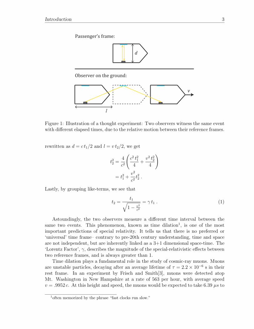
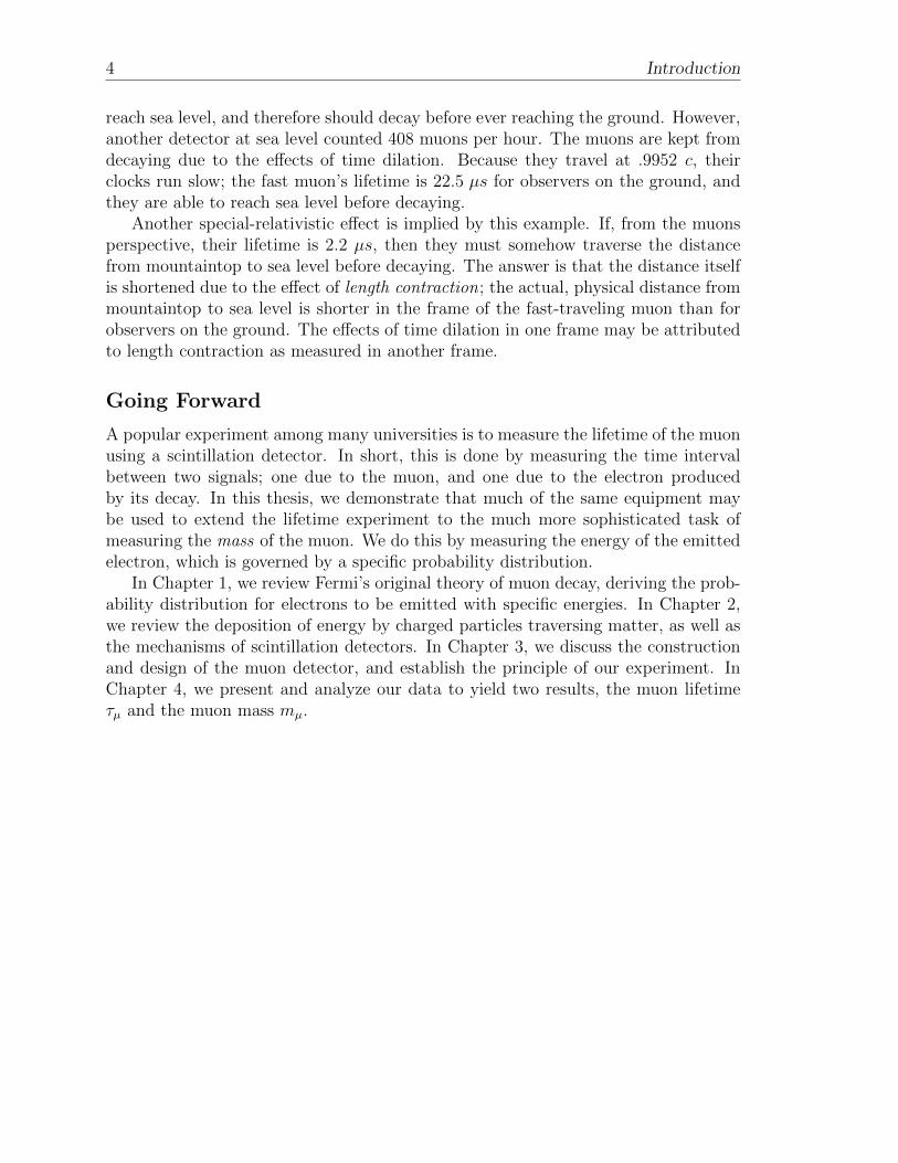
1.1 A muon at rest decays into an electron, a muon neutrino, and anelectron antineutrino. . . . . . . . . . . . . . . . . . . . . . . . . . . . 5
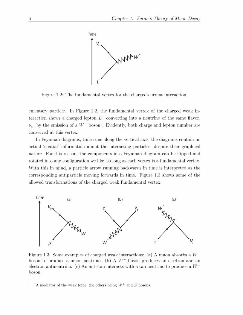
1.2 The fundamental vertex for the charged-current interaction. . . . . . 6
1.3 Some examples of charged weak interactions: (a) A muon absorbs aW+ boson to produce a muon neutrino. (b) A W− boson produces anelectron and an electron antineutrino. (c) An anti-tau interacts with atau neutrino to produce a W+ boson. . . . . . . . . . . . . . . . . . . 6
1.4 The principal (most probable) decay mode of the muon, µ− → e−+νµ+νe. 7
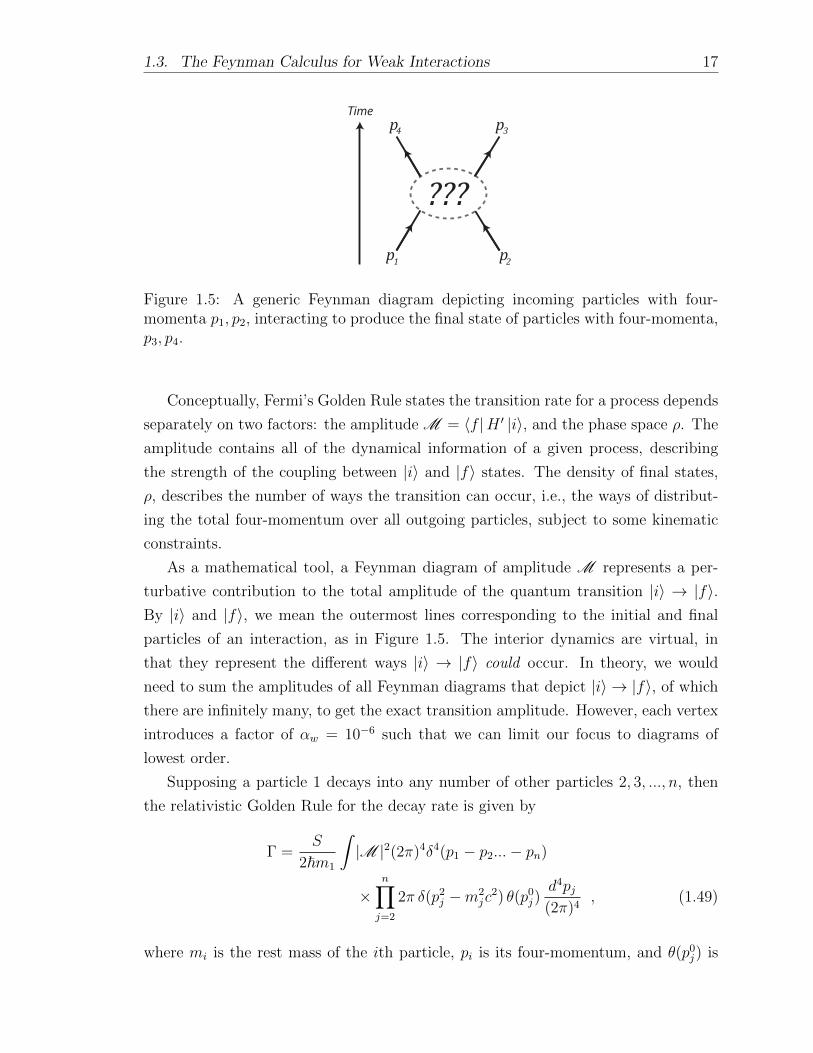
1.5 A generic Feynman diagram depicting incoming particles with four-momenta p1, p2, interacting to produce the final state of particles withfour-momenta, p3, p4. . . . . . . . . . . . . . . . . . . . . . . . . . . . 17
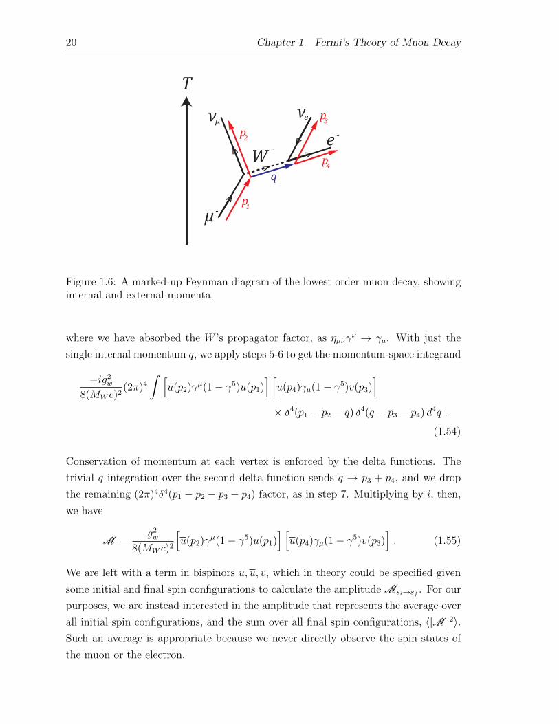
1.6 A marked-up Feynman diagram of the lowest order muon decay, show-ing internal and external momenta. . . . . . . . . . . . . . . . . . . . 20
1.7 Spectrum of e± energy in µ± decays, as predicted by the lowest-orderFeynman diagram (dotted) and with first-order radiative corrections(solid). Energies are normalized to Emax. . . . . . . . . . . . . . . . . 26
2.1 A particle incident in area dσ is scattered into solid angle dΩ. . . . . 27
2.2 The electric field of a moving point charge is distorted by the Lorentztransformation. . . . . . . . . . . . . . . . . . . . . . . . . . . . . . . 31
2.3 The collisional, radiative, and total stopping power of electrons andpositrons in polyvinyltoluene-based scintillator, calculated from theNIST EStar database. . . . . . . . . . . . . . . . . . . . . . . . . . . 35
2.4 Probability density functions modeling energy loss fluctuations in thick(left) and thin (right) absorbers. On the left, the number of large-energy-transfer collisions is small compared to the total number ofcollisions; the pdf is approximately Gaussian. On the right, large-energy-transfer collisions skew the pdf such that the mean and mostprobable energy loss no longer coincide: ∆p 6= 〈∆〉. . . . . . . . . . . 36
2.5 Energy level diagram of excitation and luminescence processes in anorganic molecule with π-electronic structure. (From H. Xu, R. Chen, Q.
Sun, W. Lai, Q. Su, W. Huang, and X. Liu, Recent progress in metal-organic
complexes for optoelectronic applications, Chem. Soc. Rev. 2014, 43, 3259-3302.
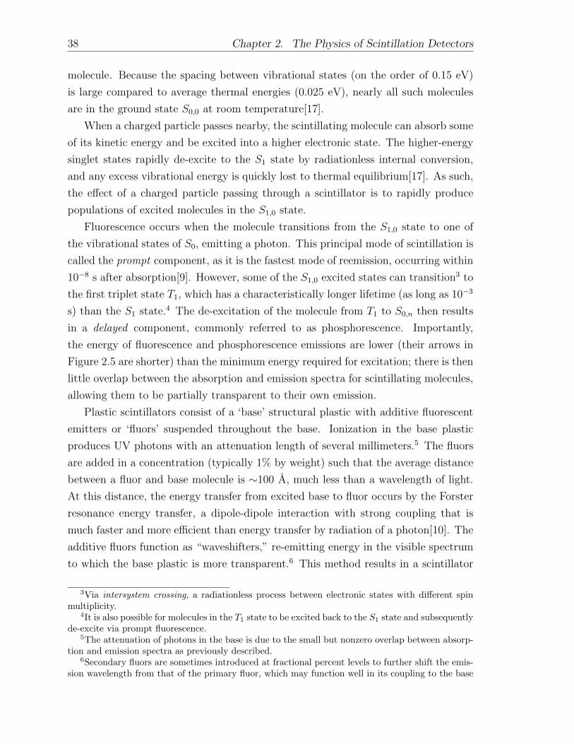
Published online 2/17/2014, Creative Commons License.) . . . . . . . . . . . 372.6 The working mechanism of a ternary-solution plastic scintillator, with
approximate fluor concentrations (in weight percentage) and energytransfer distances of the sub-processes. (From K.A. Olive et al. (Particle
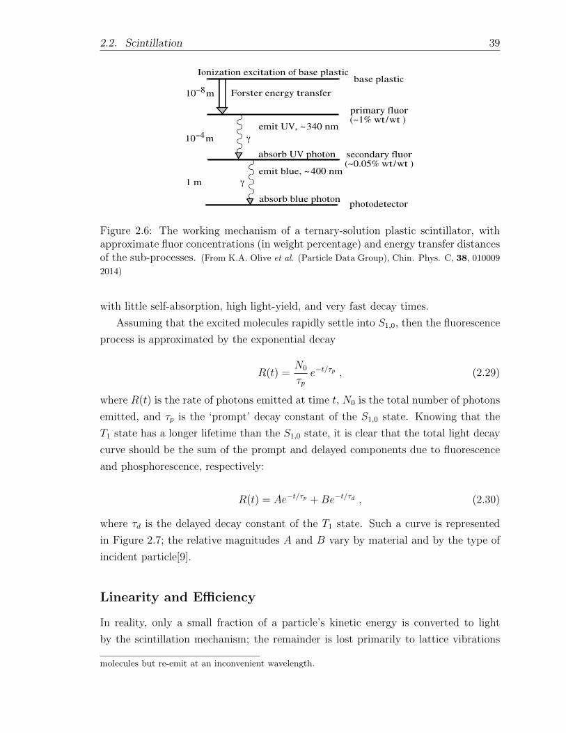
Data Group), Chin. Phys. C, 38, 010009 2014) . . . . . . . . . . . . . . . . 392.7 The composite light yield of a scintillator, represented by the sum of
two exponential decays– the prompt and delayed components. . . . . 402.8 Basic elements of a photomultiplier tube. . . . . . . . . . . . . . . . . 412.9 Left: Probability distributions of secondary electron emission at the
first dynode of a PMT, due to 1,2,3, and 4 incident photoelectrons.Statistical broadening of P (N) increases as the number of photoelec-trons increases. Right: Low-end of a simulated pulse height spectrumof a PMT. At low pulse heights, the dependence on the first dynode’sδ results in distinguishable peaks corresponding to 1, 2, and 3 photo-electron events. . . . . . . . . . . . . . . . . . . . . . . . . . . . . . . 44
3.1 Compensating the light collection for near-PMT events by a reflectiveshield. . . . . . . . . . . . . . . . . . . . . . . . . . . . . . . . . . . . 46
3.2 The PMT’s dynode output signal for two events: (a) A muon passingstraight through the detector, and (b) A muon enters with low energy,is brought to rest, and decays to produce an electron, which generatesa second pulse. . . . . . . . . . . . . . . . . . . . . . . . . . . . . . . 47
3.3 The energy spectra of e± emitted in muon decay, in an ‘ideal’ scintil-lator with infinite volume (left) and the ‘real’ scintillator with finitevolume (right). The effect of electron-escape obscures the underlyingdistribution of energy, P (e±). . . . . . . . . . . . . . . . . . . . . . . 48
3.4 Global and local coordinate conventions in the Monte Carlo transportprogram. . . . . . . . . . . . . . . . . . . . . . . . . . . . . . . . . . . 50
3.5 A particle with initial trajectory w is scattered at the origin by someangle θs, and rotated by φs. The new trajectory, θ′, φ′, is determinedby calculating the polar angle between Z and α, and the azimuthalangle between X and the projection of α into the X − Y plane. . . . 51
3.6 Mean free paths for the production of δ-rays with T > Tcut by e± withtotal energies from 2.011 - 50 MeV (positrons) and from 3.511-50 MeV(electrons). By imposing the limit Tcut = 1.5 MeV, the mean free pathis of the same length scale as the detector, and so the number of δ-raysproduced will not be too large. . . . . . . . . . . . . . . . . . . . . . . 52
3.7 A particle of kinetic energy Ek and mass m transfers kinetic energy Tto a particle with the same mass initially at rest. After collision, theincident particle is scattered by θs, and the target particle is scatteredby θr. . . . . . . . . . . . . . . . . . . . . . . . . . . . . . . . . . . . 54
3.8 Plot of Vavilov’s κ parameter for e± traveling in PVT-based scintil-lator. Because κ < 10 for energies in the range .511 − 55 MeV, weuse the Landau-Vavilov most probable energy loss, rather than theBethe-Bloch mean energy loss. . . . . . . . . . . . . . . . . . . . . . . 55
3.9 Simulated particle tracks for 20 electrons with the same initial config-uration, starting from the red dot at 0, 39 with trajectory π, 0 andtotal energy 50.511 MeV. Primary electron paths are colored in black,while δ-ray paths are colored in blue. For this simulation, Ecut = .5MeV, Tcut = 1.5 MeV, and s = .2 cm. Every simulated particle de-posited its available 50 MeV within the detector. . . . . . . . . . . . . 58
4.1 Experimental distributions of normalized e± energy, χ. There are 4291events in the set collected with the PMT operating at 1200V, and 3286events from the set collected at 1000V. Both distributions have 30 bins. 61
4.2 Renormalized distribution of the 1500 lowest-energy events from the1200V-data, in 15 bins (black) and with an interpolation of the distri-bution overlaid (red). We can distinguish the characteristic peaks of1,2, and 3-photoelectron events, for which the statistical broadening ofδ at the first dynode is small, as described in Chapter 2. . . . . . . . 62
4.3 Sum of squared residuals between the mµ = 105 simulated distributionand the experimental distribution with increasing cuts to the high-energy range (Left), and plots of the closest agreement between ex-perimental and simulated distributions, when ncuts = 11 (Right). Theexperimental distribution is plotted in Black, and the simulated dis-tribution is plotted in Cyan. The simulated distribution is generatedfrom 100000 events, and normalized to the size of the experimentaldistribution after high-range cuts. . . . . . . . . . . . . . . . . . . . . 65
4.4 Left: Experimental distribution of normalized energy χ from 1200V-data (Black) plotted with simulated distributions assuming differentvalues for mµ (Color). Right: The sum of squared residuals betweenthe experimental distribution and simulated distributions at differentvalues of mµ. We see that mµ = 105 MeV produces the strongest agree-ment (minimum residuals) between observed and simulated results, inagreement with the known value mµ = 105.6583715±0.0000035 MeV[21]. 66
4.5 Left: Experimental energy distribution from 1000V-data (Black) plot-ted with simulated distributions at different values of mµ (Color). Thevertical dotted line represents the threshold χ, above which we calcu-late the residuals. Right: The sum of squared residuals over the 9 high-est bins between experimental and simulated distributions. mµ = 105MeV produces the strongest agreement between observed and simu-lated results, and supports the same finding from the 1200V-data. . . 67
4.6 Histogram of decay times ∆t separating candidate signals of two-pulseevents in the 1000V-data. Fitting this histogram to an exponentialfunction (Red) gives us that the observed muon lifetime is τµ ≈ 2.193×10⁻⁶ s. . . . . . . . . . . . . . . . . . . . . . . . . . . . . . . . . . . . 68

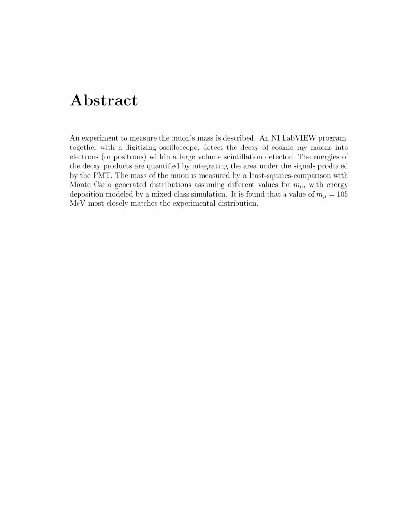
Abstract
An experiment to measure the muon’s mass is described. An NI LabVIEW program,together with a digitizing oscilloscope, detect the decay of cosmic ray muons intoelectrons (or positrons) within a large volume scintillation detector. The energies ofthe decay products are quantified by integrating the area under the signals producedby the PMT. The mass of the muon is measured by a least-squares-comparison withMonte Carlo generated distributions assuming different values for mµ, with energydeposition modeled by a mixed-class simulation. It is found that a value of mµ = 105MeV most closely matches the experimental distribution.

Introduction
Origins
On August 7, 1912, Victor Hess and two colleagues carried three electrometers ina free-balloon flight to an altitude of 5300 meters[1] and found that the ionizationrate increased nearly fourfold over that at sea level, suggesting a powerful radiationsource was at all times striking the atmosphere from space. Hess and his colleaguesruled out the Sun as a potential radiation source by repeating the balloon ascentsover several days and nights, and once even during a solar eclipse. In his words, “Theresults of my observation are best explained by the assumption that a radiation ofvery great penetrating power enters our atmosphere from above.” For their meticulousefforts, Victor Hess and colleague Carl Anderson received the Nobel Prize in Physicsin 1936.
This radiation was first thought to be high-energy photons or rays, until it wasdiscovered that their intensity varied with latitude, indicating that they were deflectedby Earth’s magnetic field and therefore were charged particles, not photons. Indeed,almost 79% of cosmic rays reaching the top of Earth’s atmosphere are protons, 15%are helium nuclei, and the remainder are mostly electrons or heavier nuclei such ascarbon, oxygen, and iron that are synthesized in stars[2].
Cosmic rays travel to us over tremendous interstellar distances, accelerated tonear the speed of light by electric fields in space. Earth’s atmosphere is constantlybombarded by these high-energy cosmic rays, the most energetic of which have 40million times the energy of particles produced at the Large Hadron Collider. Onreaching the upper atmosphere, they collide with air molecules to produce fantasticcascades of secondary particles called ‘air showers’.
The particles in these air showers continue to travel towards the Earth’s surface,decaying into lighter and lighter generations of matter. At sea level, the majority ofparticles to reach us are muons, which are essentially heavier, unstable cousins of theelectron. These cosmic muons have long been utilized as a free source of particlesfor the study of elementary particle physics, astronomy, and atmospheric physics.A popular figure among experimentalists is the rate of muons passing through youropened hand at sea level: approximately 1 per second.
Cosmic Muons and Time Dilation
The dawn of modern physics in the early 20th century was marked by a series ofsurprising discoveries that led to significant paradigm shifts. Many would argue that
2 Introduction
the advents of quantum mechanics and special relativity are the most important;the term modern physics itself is used when either of these theories is incorporated.At its heart, modern physics is the physics of extreme conditions; where quantummechanics describes the particles that make up our world at low energies and onunbelievably tiny scales, special relativity describes the behavior of space and timeat high speeds, comparable to that of light. Picturing physics in these realms, theextremely small and the extremely fast, is often entirely counterintuitive, and thereare some surprising predictions to be found therein.
In the year 1905, Albert Einstein revolutionized our view of space and time whenhe introduced his theory of special relativity. His paper “On the Electrodynamics ofMoving Bodies” used two straightforward postulates to derive the laws of special rel-ativity with straightforward trigonometry. The first postulate, attributed to Galileo,is the principle of relativity, which states that the laws of physics are the same in allinertial (non-accelerated) reference frames. A dropped ball falls the same way insidea train-car as it does for someone standing on the ground next to the tracks, exceptif the train hits a bump or goes into a turn. The second postulate, supported bythe null result of the Michelson-Morley experiment, is the constancy of the speed oflight; light always travels through a vacuum at a constant speed c, independent ofthe motion of the light source and the same for all observers.
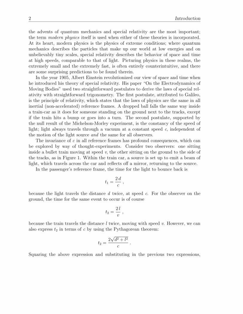
The invariance of c in all reference frames has profound consequences, which canbe explored by way of thought-experiments. Consider two observers: one sittinginside a bullet train moving at speed v, the other sitting on the ground to the side ofthe tracks, as in Figure 1. Within the train car, a source is set up to emit a beam oflight, which travels across the car and reflects off a mirror, returning to the source.
In the passenger’s reference frame, the time for the light to bounce back is
t1 =2 d
c,
because the light travels the distance d twice, at speed c. For the observer on theground, the time for the same event to occur is of course
t2 =2 l
v,
because the train travels the distance l twice, moving with speed v. However, we canalso express t2 in terms of c by using the Pythagorean theorem:
t2 =2√d2 + l2
c.
Squaring the above expression and substituting in the previous two expressions,
Introduction 3
d
v
l
Passenger’s frame:
Observer on the ground:
Figure 1: Illustration of a thought experiment: Two observers witness the same eventwith different elapsed times, due to the relative motion between their reference frames.
rewritten as d = c t1/2 and l = v t2/2, we get
t22 =4
c2
(c2 t21
4+v2 t22
4
)
= t21 +v2
c2t22 .
Lastly, by grouping like-terms, we see that
t2 =t1√
1− v2
c2
= γ t1 . (1)
Astoundingly, the two observers measure a different time interval between thesame two events. This phenomenon, known as time dilation1, is one of the mostimportant predictions of special relativity. It tells us that there is no preferred or‘universal’ time frame– contrary to pre-20th century understanding, time and spaceare not independent, but are inherently linked as a 3+1 dimensional space-time. The‘Lorentz Factor’, γ, describes the magnitude of the special-relativistic effects betweentwo reference frames, and is always greater than 1.
Time dilation plays a fundamental role in the study of cosmic-ray muons. Muonsare unstable particles, decaying after an average lifetime of τ = 2.2× 10⁻⁶ s in theirrest frame. In an experiment by Frisch and Smith[3], muons were detected atopMt. Washington in New Hampshire at a rate of 563 per hour, with average speedv = .9952 c. At this height and speed, the muons would be expected to take 6.39 µs to
1often memorized by the phrase “fast clocks run slow.”
4 Introduction
reach sea level, and therefore should decay before ever reaching the ground. However,another detector at sea level counted 408 muons per hour. The muons are kept fromdecaying due to the effects of time dilation. Because they travel at .9952 c, theirclocks run slow; the fast muon’s lifetime is 22.5 µs for observers on the ground, andthey are able to reach sea level before decaying.
Another special-relativistic effect is implied by this example. If, from the muonsperspective, their lifetime is 2.2 µs, then they must somehow traverse the distancefrom mountaintop to sea level before decaying. The answer is that the distance itselfis shortened due to the effect of length contraction; the actual, physical distance frommountaintop to sea level is shorter in the frame of the fast-traveling muon than forobservers on the ground. The effects of time dilation in one frame may be attributedto length contraction as measured in another frame.
Going Forward
A popular experiment among many universities is to measure the lifetime of the muonusing a scintillation detector. In short, this is done by measuring the time intervalbetween two signals; one due to the muon, and one due to the electron producedby its decay. In this thesis, we demonstrate that much of the same equipment maybe used to extend the lifetime experiment to the much more sophisticated task ofmeasuring the mass of the muon. We do this by measuring the energy of the emittedelectron, which is governed by a specific probability distribution.
In Chapter 1, we review Fermi’s original theory of muon decay, deriving the prob-ability distribution for electrons to be emitted with specific energies. In Chapter 2,we review the deposition of energy by charged particles traversing matter, as well asthe mechanisms of scintillation detectors. In Chapter 3, we discuss the constructionand design of the muon detector, and establish the principle of our experiment. InChapter 4, we present and analyze our data to yield two results, the muon lifetimeτµ and the muon mass mµ.
Chapter 1
Fermi’s Theory of Muon Decay
The principal experimental observables in particle physics are the scattering cross
section σ, which represents the probability of an incident particle to be scattered from
its target, and the decay width Γ, which represents the probability per unit time that
a given particle will decay. Our goal in this chapter is to develop an understanding
of the muon’s decay process as depicted in Figure 1.1.
μe
νμνe
-
-
Figure 1.1: A muon at rest decays into an electron, a muon neutrino, and an electronantineutrino.
Feynman Diagrams
In the Standard Model, particles interact with one another by the exchange of other
force-carrying or ‘mediating’ particles. The four known fundamental forces of nature
are the strong, electromagnetic, weak, and gravitational forces, and to each force
there belongs a physical theory and hypothetically, a mediating particle.
Feynman diagrams graphically represent the interactions of particles as arrang-
ments of ‘fundamental vertices’, at which a force-carrying particle couples to an el-
6 Chapter 1. Fermi’s Theory of Muon Decay
Time
L
νL
W-
-
Figure 1.2: The fundamental vertex for the charged-current interaction.
ementary particle. In Figure 1.2, the fundamental vertex of the charged weak in-
teraction shows a charged lepton L− converting into a neutrino of the same flavor,
νL, by the emission of a W− boson1. Evidently, both charge and lepton number are
conserved at this vertex.
In Feynman diagrams, time runs along the vertical axis; the diagrams contain no
actual ‘spatial’ information about the interacting particles, despite their graphical
nature. For this reason, the components in a Feynman diagram can be flipped and
rotated into any configuration we like, so long as each vertex is a fundamental vertex.
With this in mind, a particle arrow running backwards in time is interpreted as the
corresponding antiparticle moving forwards in time. Figure 1.3 shows some of the
allowed transformations of the charged weak fundamental vertex.
Time
μ
νμ
W-
-
νe
W
e-
- ντ
W
τ-
-(a) (b) (c)
Figure 1.3: Some examples of charged weak interactions: (a) A muon absorbs a W+
boson to produce a muon neutrino. (b) A W− boson produces an electron and anelectron antineutrino. (c) An anti-tau interacts with a tau neutrino to produce a W+
boson.
1A mediator of the weak force, the others being W+ and Z bosons.
7
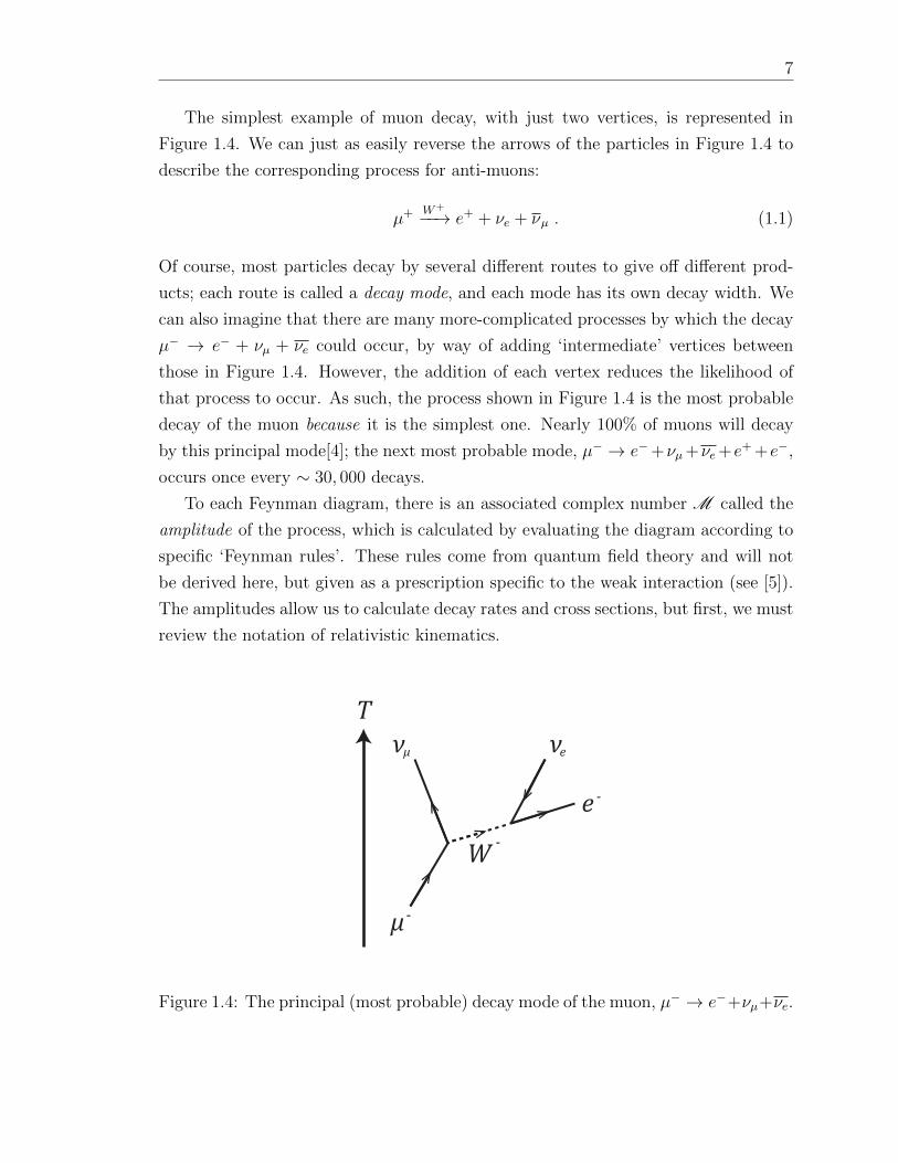
The simplest example of muon decay, with just two vertices, is represented in
Figure 1.4. We can just as easily reverse the arrows of the particles in Figure 1.4 to
describe the corresponding process for anti-muons:
µ+ W+
−−→ e+ + νe + νµ . (1.1)
Of course, most particles decay by several different routes to give off different prod-
ucts; each route is called a decay mode, and each mode has its own decay width. We
can also imagine that there are many more-complicated processes by which the decay
µ− → e− + νµ + νe could occur, by way of adding ‘intermediate’ vertices between
those in Figure 1.4. However, the addition of each vertex reduces the likelihood of
that process to occur. As such, the process shown in Figure 1.4 is the most probable
decay of the muon because it is the simplest one. Nearly 100% of muons will decay
by this principal mode[4]; the next most probable mode, µ− → e−+νµ+νe+e+ +e−,
occurs once every ∼ 30, 000 decays.
To each Feynman diagram, there is an associated complex number M called the
amplitude of the process, which is calculated by evaluating the diagram according to
specific ‘Feynman rules’. These rules come from quantum field theory and will not
be derived here, but given as a prescription specific to the weak interaction (see [5]).
The amplitudes allow us to calculate decay rates and cross sections, but first, we must
review the notation of relativistic kinematics.
T
μ
ν
e
νμ e
-
-
W -
Figure 1.4: The principal (most probable) decay mode of the muon, µ− → e−+νµ+νe.
8 Chapter 1. Fermi’s Theory of Muon Decay
1.1 Relativistic Kinematics
Knowing that time cannot be separated from the three dimensions of space (as in
the classical sense), we need new language for describing the behavior of particles
in a 3+1 dimensional spacetime. This unification is carried out in the selection of a
‘four-vector’ such that all four coordinates share the same units. By this definition,
a point in 4D spacetime is assigned its position-time four-vector xµ, as:
xµ = (x0, x1, x2, x3) = (ct, x, y, z) . (1.2)
In this notation, a Lorentz transformation between inertial reference frames S → S ′,
with S ′ moving at velocity v relative to S along the x-axis, takes the form of a matrix
multiplication as
xµ′=
3∑ν=0
Λµν x
ν −→ xµ′= Λµ
ν xν (1.3)
where on the right (and from here forward) we adopt Einstein’s summation conven-
tion, in which summation is implied over Greek indices that appear twice in one term,
one as subscript and one as superscript. The Lorentz transformation is encoded in
the coefficients of the matrix Λ,
Λ =
γ −γβ 0 0
−γβ γ 0 0
0 0 1 0
0 0 0 1
(1.4)
and any such vector that transforms as xµ in (1.3) is then called a four-vector.
In the same sense that the magnitude of a Euclidean vector pointing from a to
b in 3D space is invariant to rotations and translations, i.e. the distance between
two points is the same for any ‘observer’, the magnitude of a four-vector should be
preserved by the Lorentz transformations. To this end, we define the scalar product
of two four-vectors, aµ and bµ, as
aµbµ = a0b0 − a1b1 − a2b2 − a3b3 = aµbµ (1.5)
where contravariant four-vectors (aµ) are ‘index-up’, and covariant four-vectors are
index-down (bµ), in keeping consistent with Einstein’s summation convention. The
quantity (1.5) is the same number in all inertial reference frames.
The raising and lowering of four-vector indices is accomplished by using the
1.1. Relativistic Kinematics 9
Minkowski metric ηµν , a second-rank tensor, as
aµ = ηµν aν and aµ = ηµν aν , (1.6)
where, in the timelike convention2,
ηµν =
1 0 0 0
0 −1 0 0
0 0 −1 0
0 0 0 −1
= (ηµν)−1 = ηµν . (1.7)
Four-Vectors
The position-time four-vector, or simply the ‘four-position’, is but one example of a
four-vector. To reiterate, any object with four coordinates that transforms as xµ does
in (1.3) is a four-vector. Other properties such as the invariance of the scalar product
aµbµ follow from this one condition.
We can express many other useful quantities in four-vector form. To extend our
understanding of xµ, consider the notion of proper time (τ) as the time elapsed be-
tween two events, as measured by an observer passing through those events. Relative
to another observer’s time t, the proper time would be slowed as
dτ =dt
γ, (1.8)
which is just a restatement of ‘fast clocks run slow’. Importantly, proper time is
an invariant quantity, which motivates the idea of a proper velocity four-vector (or
simply four-velocity):
ηµ =dxµ
dτ= γ(c, vx, vy, vz) , (1.9)
where vx, vy, vz are just the components of velocity as measured in some observer’s
frame.
Naturally, we can then express momentum as a four-vector
pµ = m0ηµ = (
E
c, px, py, pz) (1.10)
where E refers to the particle’s relativistic energy (in terms of both its relativistic
2By this, we mean that the four-vector aµ is timelike if aµaµ > 0.
10 Chapter 1. Fermi’s Theory of Muon Decay
and rest masses, m and m0),
E = mc2 = (γm0)c2 =m0c
2√1− v2/c2
. (1.11)
The four-vector in (1.10) is the energy-momentum four-vector, or simply the four-
momentum.
The invariance of four-vectors is associated with certain physical ideas. Consider
the squared length of the four-momentum,
pµpµ = (m0)2 ηµη
µ
= (m0)2 γ2(c2 − (v2x + v2
y + v2z))
= (m0)2 γ2c2(1− v2/c2)
= (m0c)2 (1.12)
which also may be written
pµpµ = (E2/c2)− (p2
x + p2y + p2
z)
= (E2/c2)− p2 . (1.13)
The invariance of the length of the four-momentum, as expressed in (1.12) and (1.13),
yields the relativistic energy-momentum relation
E2 = p2c2 +m20c
4 , (1.14)
which relates an object’s rest mass m0 to its total energy E and momentum p. That
is, the length of pµ is given by m0c. The invariance of this length is associated with
the fact that m0 is the same in all reference frames.
1.2 Dirac Particles
The Dirac equation is a relativistic wave equation that describes charged, massive,
spin-1/2 particles (such as electrons). It can be derived by ‘factoring’ the relativistic
energy-momentum relation,
pµpµ − (m0c)2 = 0 , (1.15)
1.2. Dirac Particles 11
into the form of:
pµpµ − (m0c)2 = 0 = (βκpκ +m0c)(γ
λpλ −m0c) . (1.16)
Expanding the right-hand expression, we have
βκγλpκpλ −m0c(βκ − γκ)pκ − (m0c)
2 = 0 , (1.17)
where βκ and γκ are each a set of four coefficients. To eliminate terms linear in pκ,
we must have βκ = γκ, which then requires that
γκγλpκpλ − (m0c)2 = 0 . (1.18)
To find suitable coefficients γκ such that
pµpµ = γκγλpκpλ = (γκpκ)(γλpλ) (1.19)
requires that the elements of γ be matrices, and not coefficients. That is, we must
not only have (γ0)2 = 1 and (γi)2 = −1 for i = 1, 2, 3, but also that γκγλ + γλγκ = 0
for κ 6= λ, i.e., the cross-terms arising from the multiplication on the right-hand side
of (1.19) should vanish. One set of matrices satisfying these conditions are:
γ0 =
(1 0
0 −1
), γi =
(0 σi
−σi 0
)(1.20)
where 1 denotes the 2×2 identity matrix, 0 is an empty 2×2 matrix, and σi(i = 1, 2, 3)
are the Pauli matrices:
σ1 =
(0 1
1 0
), σ2 =
(0 −ii 0
), σ3 =
(1 0
0 −1
). (1.21)
By reformulating the relativistic energy-momentum relation to the form of (1.16),
now a 4x4 matrix equation, we get the Dirac equation by setting one of the right-hand
factors to zero and applying the quantum substitution pµ → i~ ∂µ:
(γµpµ −m0c) = 0 → i~ γµ∂
∂xµψ −m0c ψ = 0 (1.22)
Here, ψ is now a four-element column matrix called a ‘Dirac spinor’. For compatibility
with the γµ matrix notation, we sometimes refer to ψ as a ‘bispinor’ of two components
12 Chapter 1. Fermi’s Theory of Muon Decay
ψA and ψB, which themselves each have two components:
ψ =
(ψA
ψB
)=
ψ1
ψ2
ψ3
ψ4
. (1.23)
Zero-Momentum Solutions
A particle at rest has an infinitely large de Broglie wavelength and a spatially uniform
wave function (pµψ = i~ ∂µψ = 0 for µ = 1, 2, 3). The Dirac equation (1.22) then
reduces to its first component,
i~ γ0 1
c
∂
∂tψ −m0cψ = 0 , (1.24)
or more clearly, 1 0 0 0
0 1 0 0
0 0 −1 0
0 0 0 −1
∂ψ
∂t= −im0c
2
~ψ , (1.25)
for which the solutions are:
ψ(1) = e−(im0c2/~)t
1
0
0
0
, ψ(2) = e−(im0c2/~)t
0
1
0
0
,
ψ(3) = e+(im0c2/~)t
0
0
1
0
, ψ(4) = e+(im0c2/~)t
0
0
0
1
. (1.26)
From the characteristic time dependence of a quantum state, e−iEt/~, we see that
ψ(1) and ψ(2) are positive-energy solutions, describing spin-up and spin-down elec-
trons, respectively. The ψ(3) and ψ(4) are negative-energy solutions, which we take
to represent antiparticles with positive energy. They describe spin-down and spin-up
positrons, respectively.
1.2. Dirac Particles 13
Free Motion of a Dirac Particle
We want to find plane-wave solutions to the Dirac equation, corresponding to free
particles of definite momentum, of the form
ψ(xµ) = e−ikµxµ
u(kµ) , (1.27)
for some four-vector kµ and associated bispinor u(kµ). Noting that
∂
∂xµψ(xµ) = −ikµψ(xµ) , (1.28)
the Dirac equation then reads
i~ γµ(− ikµψ(xµ)
)−m0c ψ(xµ) = 0 , (1.29)
or more simply,
(~ γµkµ −m0c)u(kµ) = 0 . (1.30)
It is then sufficient that u(kµ) satisfy (1.30) to ensure that ψ(xµ) satisfies the Dirac
equation. With the γµ matrices written in the Pauli convention (1.20), we have
γµkµ = γ0k0 − γ1k1 − γ2k2 − γ3k3
= γ0k0 − γ · k
=
(k0 −k · σk · σ −k0
)(1.31)
with k = (k1, k2, k3) and σ = (σ1, σ2, σ3). Expressing u(kµ) as a bispinor of uA and
uB, then the condition (1.30) reads
(~ γµkµ −m0c)
(uA
uB
)=
((~k0 −m0c)uA − ~(k · σ)uB
~(k · σ)uA − (~k0 +m0c)uB
), (1.32)
which must equal zero, requiring that
uA =k · σ
k0 −m0c/~uB and uB =
k · σk0 +m0c/~
uA . (1.33)
14 Chapter 1. Fermi’s Theory of Muon Decay
We substitute uB into uA to solve the simultaneous equations, which gives us
uA =(k · σ)2
(k0)2 − (m0c/~)2uA . (1.34)
Noting that
k · σ =
(k3 k1 − ik2
k1 + ik2 −k3
), (1.35)
and consequently
(k · σ)2 = k2
(1 0
0 1
), (1.36)
we see that
k2 = (k0)2 − (m0c/~)2 −→(m0c
~
)2
= kµkµ . (1.37)
This tells us that our plane-wave solution satisfies the Dirac equation so long
as kµ is associated with the particle and has a squared length of (m0c/~)2. The
energy-momentum four-vector meets these requirements,
kµ = ±pµ
~, (1.38)
where we choose pµ to be positive for for particle states and negative for antiparticle
states, providing the desired time dependence of e∓iEt/~. Free-particle solutions are
constructed by picking
uA = Nχ
uB = Nχ′ , (1.39)
where χ and χ′ are two-component spinors and N is a normalization constant. There
exist four linearly independent bispinors u(kµ) = (uA, uB)T which correspond to the
two linearly-independent choices of each of χ and χ′. That is, we pick χr and χ′r,
where r = 1, 2, as
χ1 = χ′1 =
(1
0
)and χ2 = χ′2 =
(0
1
), (1.40)
and for each choice of either uA or uB, we construct the other using our conditions
1.2. Dirac Particles 15
on u(kµ) from (1.33). This process yields two particle solutions
u1A =
(1
0
)→ u1
B =c
E +m0c2
(pz
p+
),
u2A =
(0
1
)→ u2
B =c
E +m0c2
(p−
−pz
), (1.41)
for which kµ must be positive so that uB is defined in the limit as p → 0. Likewise,
we have two antiparticle solutions with kµ negative,
u3B =
(1
0
)→ u3
A =c
E +m0c2
(pz
p+
),
u4B =
(0
1
)→ u4
A =c
E +m0c2
(p−
−pz
), (1.42)
where p± represents the complex form px ± ipy. It is customary to represent the
particle solutions by u(1) = (u1A, u
1B)T and u(2) = (u2
A, u2B)T , whereas the antiparticle
solutions are v(1) = (u4A, u
4B)T and v(2) = −(u3
A, u3B)T . The adjoint of a bispinor is
defined as u = u†γ0, v = v†γ0, where † signifies the Hermitian conjugate.
By convention, we choose the normalization condition
u(kµ)†u(kµ) = 2E
c, (1.43)
And the normalization factor is then
N =
√E +m0c2
c. (1.44)
The free-particle bispinors have the important properties of being orthogonal,
u(1)u(2) = 0 , v(1)v(2) = 0 , (1.45)
and complete,∑s=1,2
u(s)u(s) = (γµpµ +m0c) ,∑s=1,2
v(s)v(s) = (γµpµ −m0c) . (1.46)
16 Chapter 1. Fermi’s Theory of Muon Decay
The canonical free-particle solutions are then:
ψ(1)(xµ) = e−ipµxµ/~ u(1)(kµ) =
√E +m0c2
c
1
0c(pz)
E+m0c2
c(p+)E+m0c2
e−ipµxµ/~ ,
ψ(2)(xµ) = e−ipµxµ/~ u(2)(kµ) =
√E +m0c2
c
0
1c(p−)
E+m0c2
c(−pz)E+m0c2
e−ipµxµ/~ ,
ψ(3)(xµ) = eipµxµ/~ v(1)(kµ) =
√E +m0c2
c
c(p−)
E+m0c2
c(−pz)E+m0c2
0
1
eipµxµ/~ ,
ψ(4)(xµ) = eipµxµ/~ v(2)(kµ) = −
√E +m0c2
c
c(pz)
E+m0c2
c(p+)E+m0c2
1
0
eipµxµ/~ .
(1.47)
1.3 The Feynman Calculus for Weak Interactions
We want to apply our knowledge of Dirac particles to the calculation of cross sec-
tions and decay widths. These calculations are done using Fermi’s ‘Golden Rule’,
which states that the transition rate from one energy eigenstate to another due to a
perturbation is
Γi→f =2π
~|〈f |H ′ |i〉|2ρ , (1.48)
where the kinematical factor ρ is the density of final states, and 〈f |H ′ |i〉 is the matrix
element of the perturbation Hamiltonian H ′ between the initial and final states. This
equation is nonrelativistic, but its implications are worth considering in order to
better understand quantum transitions.
1.3. The Feynman Calculus for Weak Interactions 17
Timepp
p p1 2
4 3
???
Figure 1.5: A generic Feynman diagram depicting incoming particles with four-momenta p1, p2, interacting to produce the final state of particles with four-momenta,p3, p4.
Conceptually, Fermi’s Golden Rule states the transition rate for a process depends
separately on two factors: the amplitude M = 〈f |H ′ |i〉, and the phase space ρ. The
amplitude contains all of the dynamical information of a given process, describing
the strength of the coupling between |i〉 and |f〉 states. The density of final states,
ρ, describes the number of ways the transition can occur, i.e., the ways of distribut-
ing the total four-momentum over all outgoing particles, subject to some kinematic
constraints.
As a mathematical tool, a Feynman diagram of amplitude M represents a per-
turbative contribution to the total amplitude of the quantum transition |i〉 → |f〉.By |i〉 and |f〉, we mean the outermost lines corresponding to the initial and final
particles of an interaction, as in Figure 1.5. The interior dynamics are virtual, in
that they represent the different ways |i〉 → |f〉 could occur. In theory, we would
need to sum the amplitudes of all Feynman diagrams that depict |i〉 → |f〉, of which
there are infinitely many, to get the exact transition amplitude. However, each vertex
introduces a factor of αw = 10−6 such that we can limit our focus to diagrams of
lowest order.
Supposing a particle 1 decays into any number of other particles 2, 3, ..., n, then
the relativistic Golden Rule for the decay rate is given by
Γ =S
2~m1
∫|M |2(2π)4δ4(p1 − p2...− pn)
×n∏j=2
2π δ(p2j −m2
jc2) θ(p0
j)d4pj(2π)4
, (1.49)
where mi is the rest mass of the ith particle, pi is its four-momentum, and θ(p0j) is
18 Chapter 1. Fermi’s Theory of Muon Decay
the Heaviside step-function. The S factor corrects for double-counting of identical
particles in the final state:
S =N∏i=1
1
si!(1.50)
where si is the number of particles of species i, in a process that produces N distinct
particle species.
The Feynman rules tell us how to construct M for a given Feynman diagram.
These can be derived from the Lagrangian density in quantum field theory, but here,
will simply be given as prescription. The process is:
1. Assign a momentum pi to each external line, and qi to each internal line. Draw
an arrow next to every line, running forward in time.
2. Incoming external lines contribute a factor of u or v for leptons and antileptons,
respectively. Outgoing external lines contribute u or v , again for leptons and
antileptons.
3. Each vertex contribues a factor of
−igw2√
2γµ(1− γ5) (1.51)
for weak coupling constant3 gw =√
4παw and γ5 ≡ iγ0γ1γ2γ3 =
(0 1
1 0
).
4. Each internal line contributes a propagator factor as
P (W±) =−i(ηµν − qµqν/M2c2)
qµqµ −M2c2
for W± bosons with rest mass M, and
P (L,L) =i(γµqµ +m0c)
qµqµ −m20c
2
for leptons or anti-leptons. If qµqµ (Mc)2, then the propagator of the W±
becomes
P (W±) −→ iηµν(MW c)2
,
which, for low energies, is a safe approximation (MW = 80.4± .03 GeV/c2).
3gw ≈ .6295 [5]
1.4. Decay of the Muon 19
5. For each vertex, write a delta function of the form
(2π)4δ4(k1 + k2 + k3) ,
where the k’s are the three four-momenta that form the vertex. If an arrow
points away from the vertex, then its k = −(qµ or pµ).
6. For each internal momentum qi, add a factor of
d4qi(2π)4
and integrate.
7. Cancel the resulting factor of
(2π)4δ4(p1 + p2 + ... + pn) ,
multiply by i, and the remaining value is M .
In practice, it is best to track each particle line backwards through the diagram and
write down terms as we encounter them. This procedure ensures that the multipli-
cations of bispinors and matrices are always in correct order, resulting in a single
number.
1.4 Decay of the Muon
We first apply step 1 to the lowest order Feynman diagram of the muon’s decay, as
shown in Figure 1.6. We have an incoming lepton with p1 that contributes a factor
of u(p1), two outgoing leptons that contribute u(p2) and u(p4), and one outgoing
anti-lepton that contributes a factor of v(p3). Tracing backwards from p2 → p1, we
get a ‘sandwich’ of an external line factor, vertex factor, external line factor:
Lepton Line Factor p2 → p1 =−igw2√
2
[u(p2)γµ(1− γ5)u(p1)
](1.52)
Likewise, we trace backwards from p4 → p3 to get the term
Lepton Line Factor p4 → p3 =−igw2√
2
( i
(MW c)2
)[u(p4)γµ(1− γ5)v(p3)
](1.53)
20 Chapter 1. Fermi’s Theory of Muon Decay
T
μ
νe
νμ e
-
-
W -
p1
p2
p3
p4
q
Figure 1.6: A marked-up Feynman diagram of the lowest order muon decay, showinginternal and external momenta.
where we have absorbed the W ’s propagator factor, as ηµνγν → γµ. With just the
single internal momentum q, we apply steps 5-6 to get the momentum-space integrand
−ig2w
8(MW c)2(2π)4
∫ [u(p2)γµ(1− γ5)u(p1)
] [u(p4)γµ(1− γ5)v(p3)
]× δ4(p1 − p2 − q) δ4(q − p3 − p4) d4q .
(1.54)
Conservation of momentum at each vertex is enforced by the delta functions. The
trivial q integration over the second delta function sends q → p3 + p4, and we drop
the remaining (2π)4δ4(p1 − p2 − p3 − p4) factor, as in step 7. Multiplying by i, then,
we have
M =g2w
8(MW c)2
[u(p2)γµ(1− γ5)u(p1)
] [u(p4)γµ(1− γ5)v(p3)
]. (1.55)
We are left with a term in bispinors u, u, v, which in theory could be specified given
some initial and final spin configurations to calculate the amplitude Msi→sf . For our
purposes, we are instead interested in the amplitude that represents the average over
all initial spin configurations, and the sum over all final spin configurations, 〈|M |2〉.Such an average is appropriate because we never directly observe the spin states of
the muon or the electron.
1.4. Decay of the Muon 21
Casimir’s Trick
Squaring the amplitude, we have
|M |2 =( g2
w
8(MW c)2
)2[u(p2)γµ(1− γ5)u(p1)
] [u(p4)γµ(1− γ5)v(p3)
]×[u(p2)γν(1− γ5)u(p1)
]∗ [u(p4)γν(1− γ5)v(p3)
]∗,
(1.56)
which is expressed as two factors of the form
G1 ≡[u(p2)Γ1u(p1)
] [u(p2)Γ2u(p1)
]∗,
G2 ≡[u(p4)Γ3v(p3)
] [u(p4)Γ4v(p3)
]∗. (1.57)
We note that [u(p2)Γ2u(p1)
]∗= u†(p1)Γ†2γ
0†u(p2)
and[u(p4)Γ4v(p3)
]∗= v†(p3)Γ†4γ
0†u(p4) , (1.58)
and, inserting (γ0)2 = 1 before each Γ matrix, we get
G1 =[u(p2)Γ1u(p1)
] [u(p1)Γ2u(p2)
]and
G2 =[u(p4)Γ3v(p3)
] [v(p3)Γ4u(p4)
], (1.59)
where Γi ≡ γ0Γ†iγ0.
We are interested in summing over the spin states for these G factors. From the
completeness of the bispinors, we can combine the bracketed terms as
G′1 =∑
p1 spins
G1 = u(p2)Γ1( /p1 +m1c)Γ2u(p2) = u(p2)Qau(p2) ,
G′2 =∑
p3 spins
G2 = u(p4)Γ3( /p3 −m3c)Γ4u(p4) = u(p4)Qbu(p4) , (1.60)
where /a ≡ aµγµ. If we then sum over p2 and p4’s spin states, we can exploit the
22 Chapter 1. Fermi’s Theory of Muon Decay
orthogonality of the bispinors to eliminate off-diagonal terms:
G′′1 =∑
p2 spins
G′1 =4∑
i,j=1
Qaij
[ ∑s=1,2
us(p2)us(p2)
]ji
,
G′′2 =∑
p4 spins
G′2 =4∑
i,j=1
Qbij
[ ∑s=1,2
us(p4)us(p4)
]ji
, (1.61)
and the spin-summed G factors become the simple equations
G′′1 = Tr[Qa( /p2 +m2c)] ,
G′′2 = Tr[Qb( /p4 +m4c)] . (1.62)
By this process, we have reduced the problem to that of evaluating the trace of a
product of matrices. Returning to the amplitude, and assuming the neutrino masses
m2 and m3 are negligible, we have
∑spins
|M |2 =( g2
w
8(MW c)2
)2
G′′1 G′′2
=g4w
82(MW c)4Tr[Γ1( /p1 +m1c)Γ2( /p2)]
× Tr[Γ3( /p3)Γ4( /p4 +m4c)]
= 4( gwMW c
)4
(p1 · p3) (p2 · p4) . (1.63)
In the last step, we have omitted much of the tedious matrix arithmetic involved in
simplifying the trace expressions (see [5] for exposition). We divide by the number
of initial spin states, 2, so that we are averaging over initial spins for the muon.
Therefore,
〈|M |2〉 = 2( gwMW c
)4
(p1 · p3) (p2 · p4) . (1.64)
In the rest frame of the muon, we have
p1 = (mµc, 0, 0, 0) −→ (p1 · p3) = mµE3 , (1.65)
and also, neglecting neutrino mass (p22 = m2
νc2 ≈ 0),
(p2 + p4)2 = (mec)2 + 2(p2 · p4) . (1.66)
1.4. Decay of the Muon 23
Using conservation of momentum (p1 = p2 + p3 + p4),
(p2 + p4)2 = (p1 − p3)2 = (mµc)2 − 2(p1 · p3) , (1.67)
and finally we have
(p2 · p4) =(mµc)
2 − (mec)2
2−mµE3 . (1.68)
The spin-averaged amplitude is
〈|M |2〉 =( gwMW c
)4
m2µE3(mµc
2 − 2E3)
=(g2
wmµ
M2W c
)2
|p3|(mµc− 2|p3|) , (1.69)
where we have set me = 0. This approximation does not significantly affect the
accuracy of our calculation[5]. The decay rate, given by the golden rule, is then
dΓ =〈|M |2〉2~mµ
(2π)4δ4(p1 − p2 − p3 − p4)d3p2
(2π)32|p2|d3p3
(2π)32|p3|d3p4
(2π)32|p4|, (1.70)
and all that is left is to integrate over momentum space. By the decomposition of
δ4(p1 − p2 − p3 − p4) = δ(mµc− |p2| − |p3| − |p4|)δ3(p2 + p3 + p4) , (1.71)
we integrate over p2, where the δ3 function just restricts p2 → −(p3 + p4), giving us
dΓ =〈|M |2〉
16~mµ(2π)5δ(mµc− |p3 + p4| − |p3| − |p4|)
d3p3 d3p4
|p3 + p4| |p3| |p4|. (1.72)
Next, we integrate over p3 by fixing the polar axis along p4 and transforming to
spherical coordinates p3 = (r, θ, φ), where
d3p3 = r2 sin θ dr dθ dφ = |p3|2 sin θ d|p3| dθ dφ , (1.73)
and defining
u2 ≡ |p3 + p4|2 = |p3|2 + |p4|2 + 2|p3||p4| cos θ , (1.74)
the integral over φ simply adds a factor of 2π:
dΓ =〈|M |2〉
16~mµ(2π)4
d3p4|p4|
∫δ(mµc− u− |p3| − |p4|)
|p3|d|p3| sin θ dθu
. (1.75)
24 Chapter 1. Fermi’s Theory of Muon Decay
Under the substitution (θ → u), we have
2u du = −2|p3||p4| sin θ dθ , (1.76)
and therefore, we integrate by
dΓ =〈|M |2〉
16(2π)4~mµ
d3p4|p4|2
d|p3|∫ u+
u−
δ(mµc− u− |p3| − |p4|) du , (1.77)
where
u± ≡√|p3|2 + |p4|2 ± 2|p3||p4| =
∣∣∣|p3| ± |p4|∣∣∣ . (1.78)
Of course, the integral over du is 1 if (u− < mµc−|p3|− |p4| < u+), and 0 otherwise.
This range is equivalent to the restriction that
|p3| <mµc
2,
|p4| <mµc
2,
|p3|+ |p4| >mµc
2, (1.79)
that is, no particle can be emitted with momentum greater than mµc/2, and con-
versely, any pair must have combined energy no less than mµc/2. It is illustrative
to consider the particles in the center-of-mass frame; by conservation of momentum,
the largest energy any one particle can carry is half of the available energy (mµc2/2),
and in this case, the other two particles must be emitted diametrically opposite to
the first, such that the total momentum be zero.
By the inequalities in (1.79), we then integrate over |p3| from (mµc/2 − |p4|) to
(mµc/2):
dΓ =( g2
w
16π2M2W
)2 mµ
~c2
d3p4|p4|2
∫ mµc/2
mµc/2−|p4||p3|(mµc− 2|p3|)d|p3|
=( g2
w
16π2M2W
)2 mµ
~c2
(mµc
2− 2
3|p4|
)d3p4 , (1.80)
and, writing d3p4 = 4π|p4|2d|p4| in spherical polar form, we get
dΓ
d|p4|=( g2
w
16π2M2W
)2mµ
~c24π(mµc
2|p4|2 −
2
3|p4|3
). (1.81)
1.4. Decay of the Muon 25
Expressing this in terms of the electron energy E = |p4|c, then
dΓ
dE=( gwMW c
)4 m2µE
2
2~(4π)3
(1− 4E
3mµc2
), (1.82)
which tells us the energy distribution of the electrons emitted in muon decay. Because
dΓ/dE is independent of angle, the probability of electrons to be produced with energy
Ee in a given time interval and solid angle is
P (Ee) = C(mµc2Ee)
2(
3− 4Eemµc2
), (1.83)
for some constant value C. By integrating (1.82) over energy, the total decay rate is
Γ =( gwMW c
)4 m2µ
2~(4π)3
∫ mµc2/2
0
E2(
1− 4E
3mµc2
)dE
=(mµgwMW
)4 mµc2
12~(8π)3, (1.84)
and so the lifetime of the muon, to lowest order, is
τµ ≡1
Γ=( MW
mµgw
)4 12~(8π)3
mµc2≈ 2.532µs . (1.85)
The muon decay spectrum and lifetime predicted by this lowest-order Feynman
diagram are a close first estimate to the true behavior of muon decay. Ever since its
discovery in 1936, the muon has occupied a special role in the field of experimental
particle physics. As the only accessible, purely leptonic process, the study of muon
decay has been central to understanding weak interactions. Today, its lifetime is
known to greater accuracy than any other unstable particle; a wealth of experiments
are dedicated to measuring its properties with extremely high precision, in hopes of
finding “new physics” beyond the Standard Model[6].
The accuracy of these theoretical predictions is increased by considering the contri-
bution of higher-order processes to the overall amplitude. The next step, beyond the
lowest-order diagram, is to factor in radiative corrections arising from the exchange
of a virtual photon by the µ± and e±, which add O(α) terms. With the addition
of first-order radiative corrections, the normalized energy spectrum of electrons and
positrons in µ± decay is given by[7]
P (x) =G2Fm
5µ
96π3x2(3− 2x)
1 +
α
2π
(A(x) + ln
[m2µ
m2e
]B(x)
), (1.86)
26 Chapter 1. Fermi’s Theory of Muon Decay
First-Order RC
Lowest Order Spectrum
0.0 0.2 0.4 0.6 0.8 1.0
0.0
0.5
1.0
1.5
2.0
Normalized Energy χ
ProbablityDensity
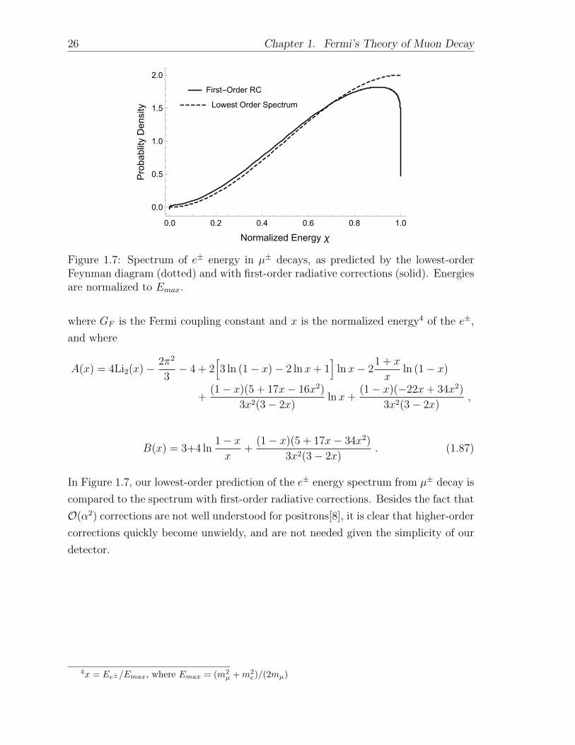
Figure 1.7: Spectrum of e± energy in µ± decays, as predicted by the lowest-orderFeynman diagram (dotted) and with first-order radiative corrections (solid). Energiesare normalized to Emax.
where GF is the Fermi coupling constant and x is the normalized energy4 of the e±,
and where
A(x) = 4Li2(x)− 2π2
3− 4 + 2
[3 ln (1− x)− 2 lnx+ 1
]lnx− 2
1 + x
xln (1− x)
+(1− x)(5 + 17x− 16x2)
3x2(3− 2x)lnx+
(1− x)(−22x+ 34x2)
3x2(3− 2x),
B(x) = 3+4 ln1− xx
+(1− x)(5 + 17x− 34x2)
3x2(3− 2x). (1.87)
In Figure 1.7, our lowest-order prediction of the e± energy spectrum from µ± decay is
compared to the spectrum with first-order radiative corrections. Besides the fact that
O(α2) corrections are not well understood for positrons[8], it is clear that higher-order
corrections quickly become unwieldy, and are not needed given the simplicity of our
detector.
4x = Ee±/Emax, where Emax = (m2µ +m2
e)/(2mµ)
Chapter 2
The Physics of Scintillation
Detectors
Here, we discuss the various components of the scintillation detector: the energy loss
of charged particles passing through matter, the production of light in scintillating
materials, and the detection of these light pulses by photomultiplier tubes.
2.1 Passage of Radiation through Matter
In particle physics, we describe the scattering of two particles in terms of the cross
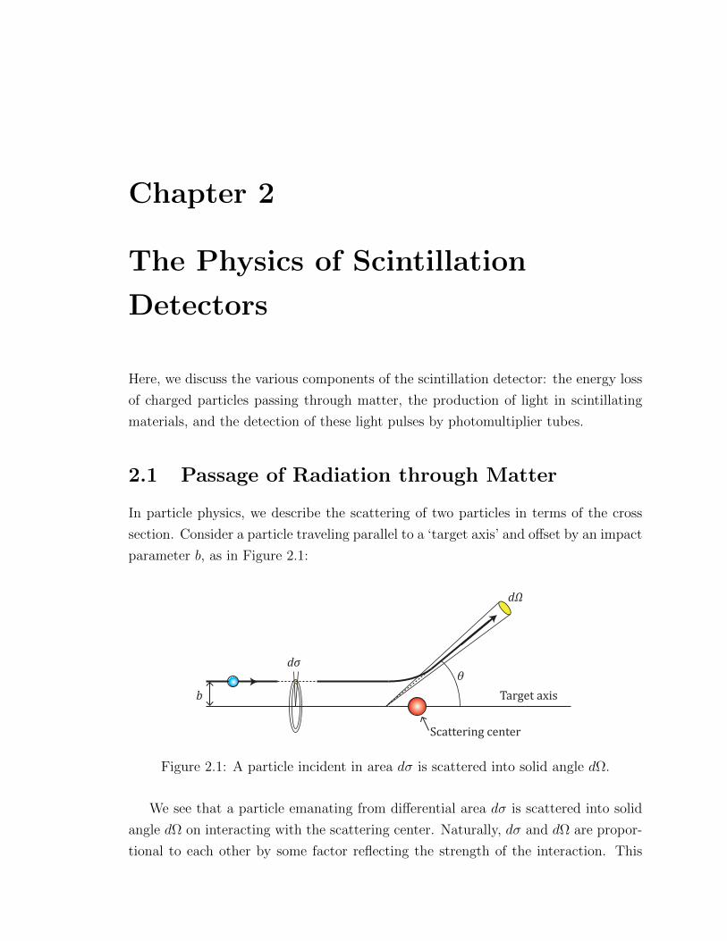
section. Consider a particle traveling parallel to a ‘target axis’ and offset by an impact
parameter b, as in Figure 2.1:
b Target axis
Scattering center
d
dσθ
Figure 2.1: A particle incident in area dσ is scattered into solid angle dΩ.
We see that a particle emanating from differential area dσ is scattered into solid
angle dΩ on interacting with the scattering center. Naturally, dσ and dΩ are propor-
tional to each other by some factor reflecting the strength of the interaction. This
28 Chapter 2. The Physics of Scintillation Detectors
proportionality factor is the differential cross section, D(θ):
D(θ) =dσ
dΩ. (2.1)
We find the total cross section by integrating D(θ) over all solid angles:
σ =
∫dσ =
∫D(θ) dΩ =
∫∫D(θ) sin θ dθ dφ . (2.2)
Of course, dσ and σ have units of area, hence the term ‘cross section’. However,
the interpretation of dσ as a geometric cross-sectional area should not be confused
with the real physical dimensions of the target. The scattering cross section is a
hypothetical area that describes the likelihood of being scattered by the target.
In real materials, we have many scattering centers instead of a single target. To
extend the example, consider a beam of particles with flux1 F and cross-sectional
area A, incident on a slab of material with a uniform number density of centers N
and thickness δx. Assuming δx is small enough that the centers have a low chance to
obscure each other, then the average number of particles scattered into solid angle
dΩ per unit time is
Ns(Ω) = (F A)(N δx)dσ
dΩ, (2.3)
and the total number of particles scattered into all angles per unit time is
Ntotal =
∫Ns(Ω) dΩ = (F A)(N δx)σ . (2.4)
Dividing by (F A), the total number of incident particles per unit time, then we
have the probability of interaction for a single particle to be scattered in traversing a
thickness δx:
Pint(δx) = (N δx)σ . (2.5)
Mean Free Path
We want to consider the ‘survival probability’ for a particle to travel some thickness
x without scattering: Ps(x). If w dx is the probability of interacting over a distance
dx, with w assumed constant, then the probability of not interacting over a length
x+ dx is
Ps(x+ dx) = Ps(x) +dPsdx
dx = Ps(x)(1− w dx) , (2.6)
1Incident particles per unit area, per time.
2.1. Passage of Radiation through Matter 29
which yieldsdPsdx
= −wPs(x) −→ Ps(x) = e−wx , (2.7)
and we see that the survival probability declines exponentially in distance. Likewise,
we can express the probability of a particle scattering within the region x to x+ dx,
after traveling x without interacting, as
dPint(x) = Ps(x)wdx = e−wxwdx . (2.8)
The mean free path, λ, is defined as the average distance traveled by a particle
between successive scattering events; this is simply the expectation value of dPint(x),
λ = 〈x〉 ≡∫ ∞
0
x dPint =
∫ ∞0
w x e−wxdx =1
w. (2.9)
Thus, putting this result into (2.7), we find that
Ps(x) = e−x/λ . (2.10)
Intuitively, λ should be related to the number density of centers N and the total
scattering cross-section of the medium, σ. In the limit of small δx, we can use the
Taylor series expansion of Pint(δx) = 1− Ps(δx) = 1− e−δx/λ:
Pint(δx) = 1−(
1− δxλ
+O(δ2x))
' δxλ, (2.11)
which, when combined with (2.5), yields λ = 1/Nσ.
2.1.1 The Bethe-Bloch Formula
The passage of charged particles through matter is generally characterized by energy
loss and path deflection due to electromagnetic interactions with the nuclei and orbital
electrons of the material. Specifically, inelastic collisions with atomic electrons may
result in their excitation or ionization; this energy comes at the expense of the incident
particle, causing it to slow down. In contrast, elastic collisions with atomic nuclei
cause the incident particle to be deflected from its initial trajectory. Because the
volume of an atom is primarily empty space, elastic scattering events from nuclei
occur less frequently than inelastic collisions with atomic electrons.
30 Chapter 2. The Physics of Scintillation Detectors
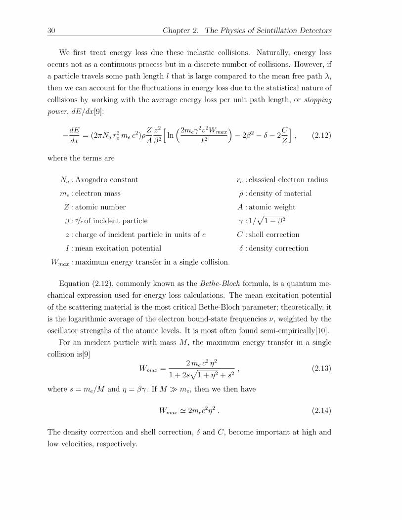
We first treat energy loss due these inelastic collisions. Naturally, energy loss
occurs not as a continuous process but in a discrete number of collisions. However, if
a particle travels some path length l that is large compared to the mean free path λ,
then we can account for the fluctuations in energy loss due to the statistical nature of
collisions by working with the average energy loss per unit path length, or stopping
power, dE/dx[9]:
−dEdx
= (2πNa r2e me c
2)ρZ
A
z2
β2
[ln(2meγ
2v2Wmax
I2
)− 2β2 − δ − 2
C
Z
], (2.12)
where the terms are
Na : Avogadro constant re : classical electron radius
me : electron mass ρ : density of material
Z : atomic number A : atomic weight
β : v/c of incident particle γ : 1/√
1− β2
z : charge of incident particle in units of e C : shell correction
I : mean excitation potential δ : density correction
Wmax : maximum energy transfer in a single collision.
Equation (2.12), commonly known as the Bethe-Bloch formula, is a quantum me-
chanical expression used for energy loss calculations. The mean excitation potential
of the scattering material is the most critical Bethe-Bloch parameter; theoretically, it
is the logarithmic average of the electron bound-state frequencies ν, weighted by the
oscillator strengths of the atomic levels. It is most often found semi-empirically[10].
For an incident particle with mass M , the maximum energy transfer in a single
collision is[9]
Wmax =2me c
2 η2
1 + 2s√
1 + η2 + s2, (2.13)
where s = me/M and η = βγ. If M me, then we then have
Wmax ' 2mec2η2 . (2.14)
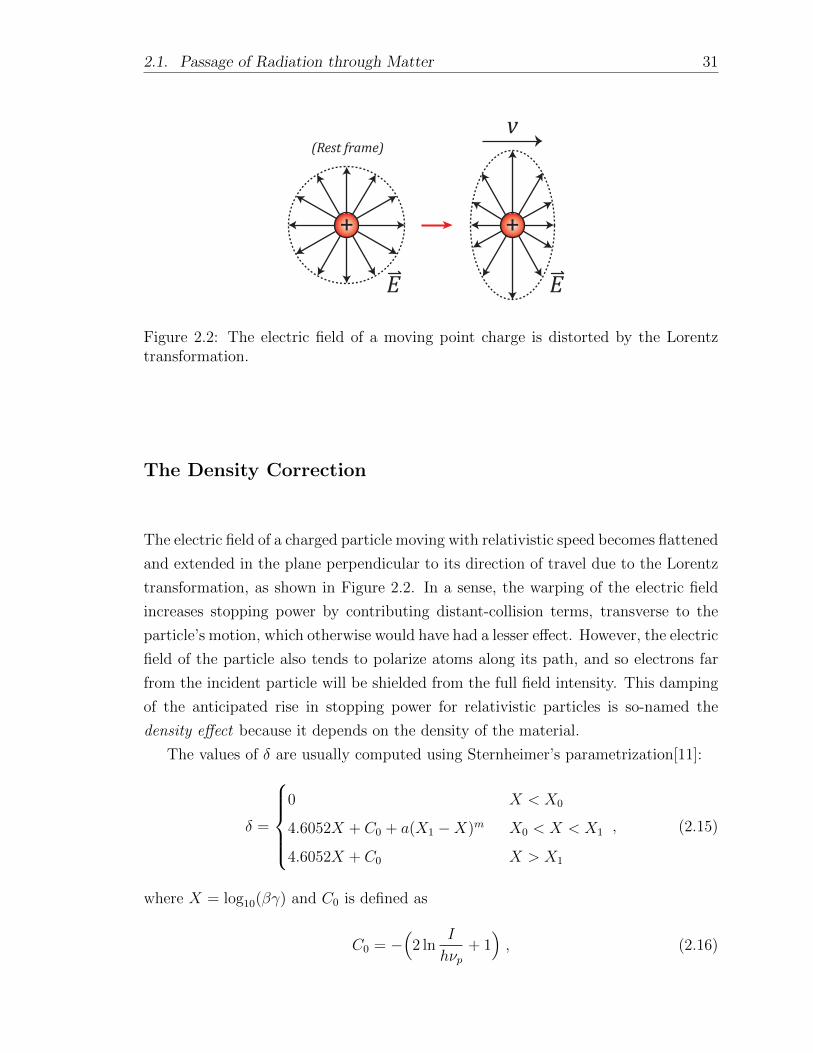
The density correction and shell correction, δ and C, become important at high and
low velocities, respectively.
2.1. Passage of Radiation through Matter 31
+ +
v
E E
(Rest frame)
Figure 2.2: The electric field of a moving point charge is distorted by the Lorentztransformation.
The Density Correction
The electric field of a charged particle moving with relativistic speed becomes flattened
and extended in the plane perpendicular to its direction of travel due to the Lorentz
transformation, as shown in Figure 2.2. In a sense, the warping of the electric field
increases stopping power by contributing distant-collision terms, transverse to the
particle’s motion, which otherwise would have had a lesser effect. However, the electric
field of the particle also tends to polarize atoms along its path, and so electrons far
from the incident particle will be shielded from the full field intensity. This damping
of the anticipated rise in stopping power for relativistic particles is so-named the
density effect because it depends on the density of the material.
The values of δ are usually computed using Sternheimer’s parametrization[11]:
δ =
0 X < X0
4.6052X + C0 + a(X1 −X)m X0 < X < X1
4.6052X + C0 X > X1
, (2.15)
where X = log10(βγ) and C0 is defined as
C0 = −(
2 lnI
hνp+ 1), (2.16)
32 Chapter 2. The Physics of Scintillation Detectors
and where hνp is the plasma frequency of the material with electron density Ne,
νp =
√Ne e2
πme
. (2.17)
The remaining parameters are found by fitting (2.15) to experimental data.
The Shell Correction
When the velocity of the particle is slowed to be comparable to the orbital velocity of
bound electrons, the electrons can no longer be assumed stationary with respect the
particle, an explicit assumption of the Bethe-Bloch formula. An empirical correction
is used in this regime[12], valid for η ≥ 0.1:
C(I, η) =(0.422377η−2 + 0.0304043η−4 − 0.00038106η−6)× 10−6I2
+ (3.850190η−2 − 0.1667989η−4 + 0.00157955η−6)× 10−9I3 , (2.18)
recalling that η = βγ and I is the mean excitation potential, in eV.
2.1.2 Energy Loss of Electrons and Positrons
Like other charged particles, electrons and positrons suffer collisional energy losses
when passing through matter. However, due to their small mass, they can lose signif-
icant energy due to the emission of electromagnetic radiation as they are decelerated
by the electric field of a nucleus. This braking radiation or bremsstrahlung quickly
dominates energy losses at energies above a few 10’s of MeV[9]. The total stopping
power is then composed of radiative and collisional losses,(dE
dx
)total
=
(dE
dx
)rad
+
(dE
dx
)coll
, (2.19)
and the material-specific critical energy Ec is defined as the energy at which radiative
and collisional losses are equal to each other.
The collisional term, based on the Bethe-Bloch formula, must be modified to
account for the fact that electrons are indistinguishable particles. In particular, the
maximum energy transfer due to a head-on collision is now Wmax = Te/2, where Te
is the kinetic energy of the incident electron[10]. Positrons, which are not subject
to this limitation, have Wmax = Tp with incident kinetic energy Tp. The modified
2.1. Passage of Radiation through Matter 33
Bethe-Bloch formula for collisional losses is then
−
(dE
dx
)coll
= (2πNa r2e me c
2)ρZ
A
1
β2
[ln(τ 2(τ + 2)(mec
2)2
2I2
)− F±(τ)− δ − 2
C
Z
],
(2.20)
where τ is the kinetic energy of the particle in units of mec2, and F (τ) is given by
F−(τ) = 1− β2 +τ2
8− (2τ + 1) ln 2
(τ + 1)2,
F+(τ) = 2 ln 2− β2
12
(23 +
14
τ + 2+
10
(τ + 2)2+
4
(τ + 2)3
), (2.21)
for electrons and positrons, respectively[9].
Radiative Losses
Because radiative losses depend on the electric field felt by the electron, the screening
of the nucleus’ electric field by atomic electrons plays an important role. As such,
the bremsstrahlung cross-section is dependent on the electron’s energy, its impact
parameter, and the atomic number of the material, Z. Screening is parametrized by
the quantity
ξ =100mec
2hν
E0EZ1/3, (2.22)
where E0 is the particle’s total initial energy and E is its final total energy, and
hν is the energy of the emitted photon. For complete screening, ξ ' 0, and for no
screening, ξ 1. The bremsstrahlung cross-section is given by the formula[9]
dσ = 4Z2r2eαdν
ν
(1 + ε)2
[φ1(ξ)
4−1
3lnZ − f(Z)
]− 2
3ε[φ2(ξ)
4− 1
3lnZ − f(Z)
], (2.23)
where ε = E/E0, α = 1/137, f(Z) is a small correction accounting for the Coulomb
interaction of the emitting electron in the electric field of the nucleus, and φ1, φ2 are
screening functions depending on ξ:
34 Chapter 2. The Physics of Scintillation Detectors
φ1(ξ) = 20.863− 2 ln[1 + (0.55846ξ)2]− 4[1− 0.6e−0.9ξ − 0.4e−1.5ξ] ,
φ2(ξ) = φ1(ξ)− 2
3(1 + 6.5ξ + 6ξ2)−1 , (2.24)
and where
f(Z) ' a2[(1 + a2)−1 + 0.20206− 0.0369a2 + 0.0083a4 − 0.002a6
](2.25)
for a = Zα.
The energy loss due to radiation is then calculated by integrating the cross section
dσ/dν times the photon energy hν over the allowed frequency range,
−
(dE
dx
)rad
= N
∫ ν0
0
hνdσ
dνdν (2.26)
where N is the number of atoms per cubic centimeter, and ν0 = E0/h.
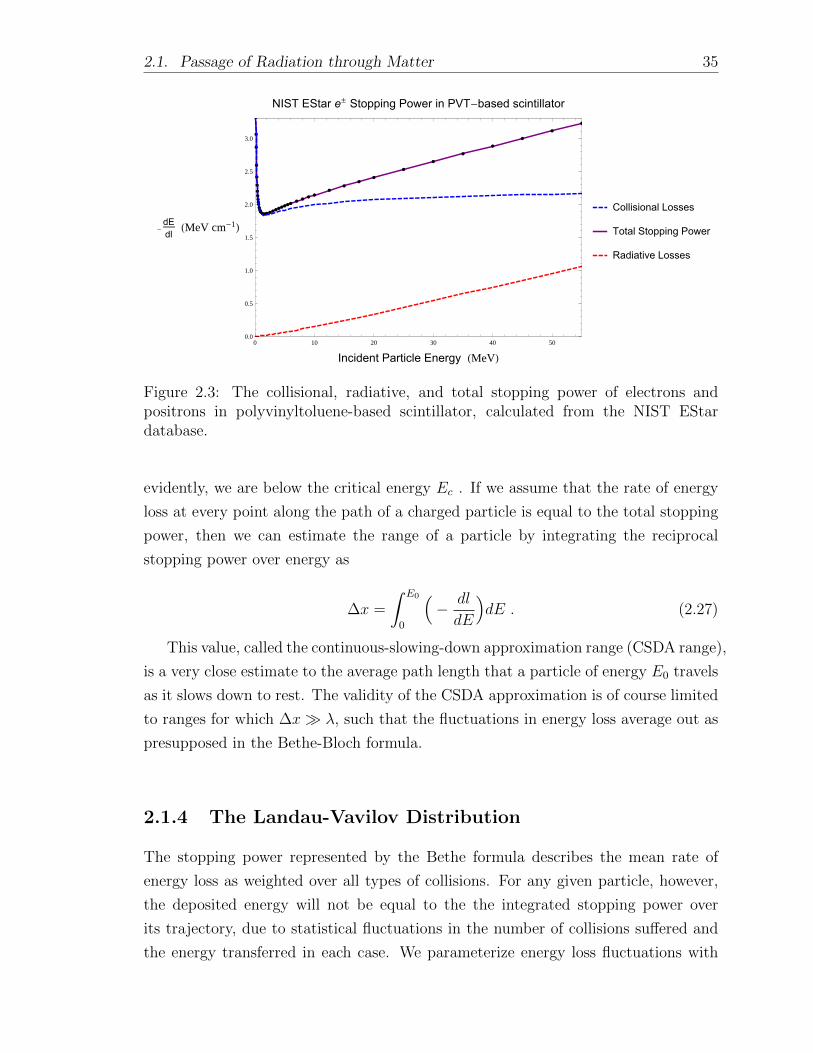
2.1.3 NIST EStar Database
The National Institute of Standards and Technology (NIST) has available three
computer-readable databases for calculating stopping power-related data. These are
EStar, PStar, and AStar, for electrons, protons, and helium ions, respectively. The
EStar program calculates collisional and radiative losses, density corrections, and the
total stopping power for electrons (or positrons) traveling through any one material
from a list of hundreds of common compounds.
The method of EStar’s calculation follows the Bethe-Bloch formula (2.20) with
the material-specific density correction (2.15) and mean excitation potential I. EStar
does not include a shell correction, meaning that collisional loss uncertainties increase
from between 1% and 2% above 100 keV, to between 5% and 10% from 100 keV to 10
keV. This is not a concern because the energy range below 100 keV is only .2% of the
range we are interested in (up to 52.5 MeV). Radiative losses are calculated through a
combination of bremsstrahlung cross sections[13], numerical results in the sub-2 MeV
range[14], analytical formulas above 50 MeV, and interpolation in the intermediate
2-50 MeV range.
In Figure 2.3, we see that the radiative losses increase for higher-energy electrons,
but that collisional losses still dominate in the range of interest below 52.5 MeV;
2.1. Passage of Radiation through Matter 35
0 10 20 30 40 50
0.0
0.5
1.0
1.5
2.0
2.5
3.0
Incident Particle Energy HMeVL
-dE
dlHMeV cm
-1L
NIST EStar e±
Stopping Power in PVT-based scintillator
Collisional Losses
Total Stopping Power
Radiative Losses
Figure 2.3: The collisional, radiative, and total stopping power of electrons andpositrons in polyvinyltoluene-based scintillator, calculated from the NIST EStardatabase.
evidently, we are below the critical energy Ec . If we assume that the rate of energy
loss at every point along the path of a charged particle is equal to the total stopping
power, then we can estimate the range of a particle by integrating the reciprocal
stopping power over energy as
∆x =
∫ E0
0
(− dl
dE
)dE . (2.27)
This value, called the continuous-slowing-down approximation range (CSDA range),
is a very close estimate to the average path length that a particle of energy E0 travels
as it slows down to rest. The validity of the CSDA approximation is of course limited
to ranges for which ∆x λ, such that the fluctuations in energy loss average out as
presupposed in the Bethe-Bloch formula.
2.1.4 The Landau-Vavilov Distribution
The stopping power represented by the Bethe formula describes the mean rate of
energy loss as weighted over all types of collisions. For any given particle, however,
the deposited energy will not be equal to the the integrated stopping power over
its trajectory, due to statistical fluctuations in the number of collisions suffered and
the energy transferred in each case. We parameterize energy loss fluctuations with
36 Chapter 2. The Physics of Scintillation Detectors
Dp=XD\
0 2 4 6 8 10 12 14
0.0
0.1
0.2
0.3
0.4
Energy Loss Ξ, HMeVL
Pro
ba
bili
tyD
en
sity
Dp XD\0 2 4 6 8 10 12 14
0.00
0.05
0.10
0.15
0.20
Energy Loss Ξ HMeVL
Pro
ba
bili
tyD
en
sity
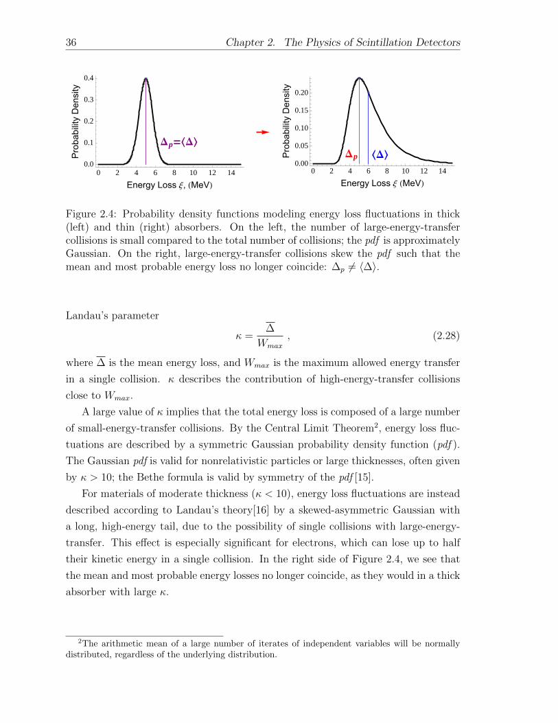
Figure 2.4: Probability density functions modeling energy loss fluctuations in thick(left) and thin (right) absorbers. On the left, the number of large-energy-transfercollisions is small compared to the total number of collisions; the pdf is approximatelyGaussian. On the right, large-energy-transfer collisions skew the pdf such that themean and most probable energy loss no longer coincide: ∆p 6= 〈∆〉.
Landau’s parameter
κ =∆
Wmax
, (2.28)
where ∆ is the mean energy loss, and Wmax is the maximum allowed energy transfer
in a single collision. κ describes the contribution of high-energy-transfer collisions
close to Wmax.
A large value of κ implies that the total energy loss is composed of a large number
of small-energy-transfer collisions. By the Central Limit Theorem2, energy loss fluc-
tuations are described by a symmetric Gaussian probability density function (pdf ).
The Gaussian pdf is valid for nonrelativistic particles or large thicknesses, often given
by κ > 10; the Bethe formula is valid by symmetry of the pdf [15].
For materials of moderate thickness (κ < 10), energy loss fluctuations are instead
described according to Landau’s theory[16] by a skewed-asymmetric Gaussian with
a long, high-energy tail, due to the possibility of single collisions with large-energy-
transfer. This effect is especially significant for electrons, which can lose up to half
their kinetic energy in a single collision. In the right side of Figure 2.4, we see that
the mean and most probable energy losses no longer coincide, as they would in a thick
absorber with large κ.
2The arithmetic mean of a large number of iterates of independent variables will be normallydistributed, regardless of the underlying distribution.
2.2. Scintillation 37
2.2 Scintillation
Scintillators are materials that respond to the energy loss of particles by reemitting
the deposited energy as light. This prompt emission of light in response to excitation
is called fluorescence; it is a property shared by all scintillators, and is the reason for
their widespread use as particle detectors.
The six primary types of scintillators in use today are: organic crystals, organic
liquids, plastics, inorganic crystals, gaseous scintillators, and glasses. Even within
each type, there are many different choices of compounds available, depending on the
intended use of the scintillator. Plastics are the general ‘workhorse’ scintillator in
nuclear and particle physics, due to their extremely fast signals, relatively cheap cost,
and the ease with which they are molded and machined into different shapes. As the
detector in this experiment uses plastic scintillator, we limit discussion to this class
of material.
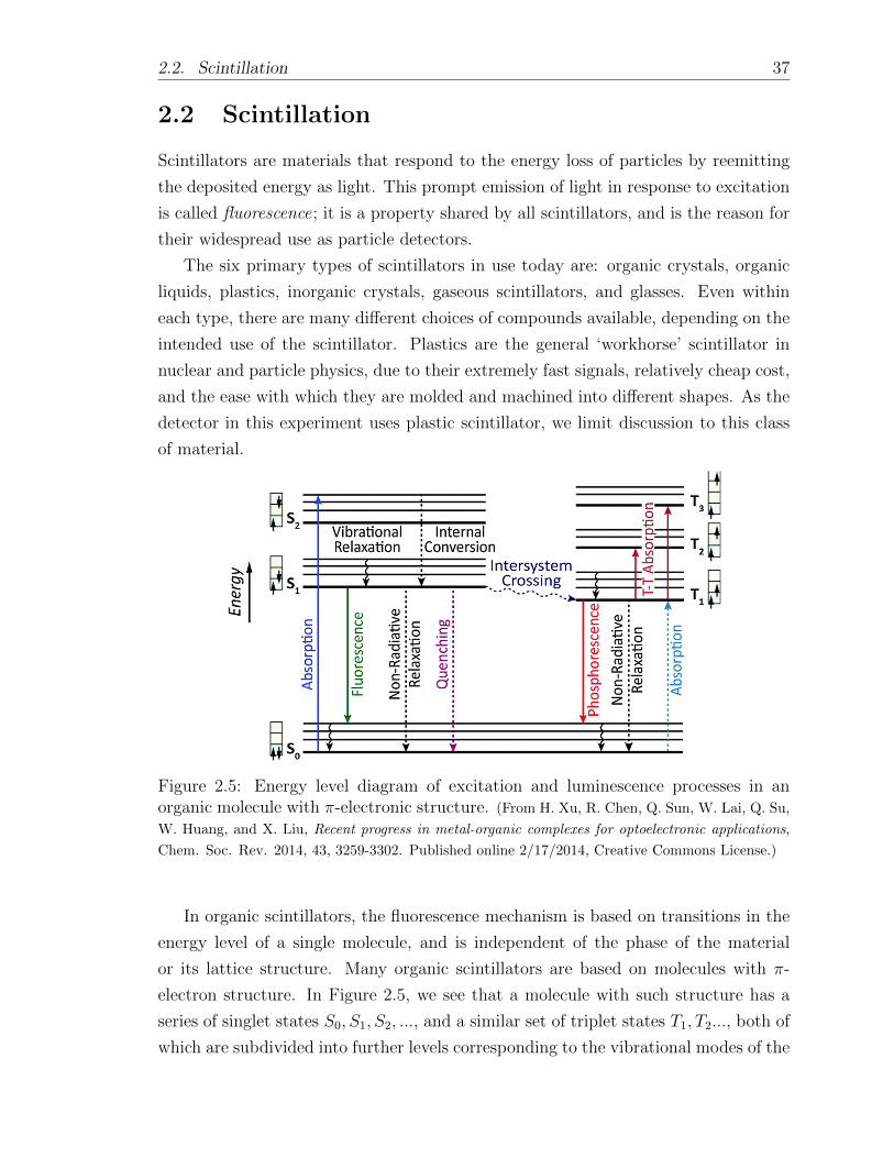
Figure 2.5: Energy level diagram of excitation and luminescence processes in anorganic molecule with π-electronic structure. (From H. Xu, R. Chen, Q. Sun, W. Lai, Q. Su,
W. Huang, and X. Liu, Recent progress in metal-organic complexes for optoelectronic applications,
Chem. Soc. Rev. 2014, 43, 3259-3302. Published online 2/17/2014, Creative Commons License.)
In organic scintillators, the fluorescence mechanism is based on transitions in the
energy level of a single molecule, and is independent of the phase of the material
or its lattice structure. Many organic scintillators are based on molecules with π-
electron structure. In Figure 2.5, we see that a molecule with such structure has a
series of singlet states S0, S1, S2, ..., and a similar set of triplet states T1, T2..., both of
which are subdivided into further levels corresponding to the vibrational modes of the
38 Chapter 2. The Physics of Scintillation Detectors
molecule. Because the spacing between vibrational states (on the order of 0.15 eV)
is large compared to average thermal energies (0.025 eV), nearly all such molecules
are in the ground state S0,0 at room temperature[17].
When a charged particle passes nearby, the scintillating molecule can absorb some
of its kinetic energy and be excited into a higher electronic state. The higher-energy
singlet states rapidly de-excite to the S1 state by radiationless internal conversion,
and any excess vibrational energy is quickly lost to thermal equilibrium[17]. As such,
the effect of a charged particle passing through a scintillator is to rapidly produce
populations of excited molecules in the S1,0 state.
Fluorescence occurs when the molecule transitions from the S1,0 state to one of
the vibrational states of S0, emitting a photon. This principal mode of scintillation is
called the prompt component, as it is the fastest mode of reemission, occurring within
10−8 s after absorption[9]. However, some of the S1,0 excited states can transition3 to
the first triplet state T1, which has a characteristically longer lifetime (as long as 10−3
s) than the S1 state.4 The de-excitation of the molecule from T1 to S0,n then results
in a delayed component, commonly referred to as phosphorescence. Importantly,
the energy of fluorescence and phosphorescence emissions are lower (their arrows in
Figure 2.5 are shorter) than the minimum energy required for excitation; there is then
little overlap between the absorption and emission spectra for scintillating molecules,
allowing them to be partially transparent to their own emission.
Plastic scintillators consist of a ‘base’ structural plastic with additive fluorescent
emitters or ‘fluors’ suspended throughout the base. Ionization in the base plastic
produces UV photons with an attenuation length of several millimeters.5 The fluors
are added in a concentration (typically 1% by weight) such that the average distance
between a fluor and base molecule is ∼100 A, much less than a wavelength of light.
At this distance, the energy transfer from excited base to fluor occurs by the Forster
resonance energy transfer, a dipole-dipole interaction with strong coupling that is
much faster and more efficient than energy transfer by radiation of a photon[10]. The
additive fluors function as “waveshifters,” re-emitting energy in the visible spectrum
to which the base plastic is more transparent.6 This method results in a scintillator
3Via intersystem crossing, a radiationless process between electronic states with different spinmultiplicity.
4It is also possible for molecules in the T1 state to be excited back to the S1 state and subsequentlyde-excite via prompt fluorescence.
5The attenuation of photons in the base is due to the small but nonzero overlap between absorp-tion and emission spectra as previously described.
6Secondary fluors are sometimes introduced at fractional percent levels to further shift the emis-sion wavelength from that of the primary fluor, which may function well in its coupling to the base
2.2. Scintillation 39
Ionization excitation of base plastic
Forster energy transfer
a
a
base plastic
primary fluor(~1% wt /wt )
secondary fluor(~0.05% wt /wt )
photodetector
emit UV, ~340 nm
absorb blue photon
absorb UV photon
emit blue, ~400 nm1 m
10<4m
10<8m
Figure 2.6: The working mechanism of a ternary-solution plastic scintillator, withapproximate fluor concentrations (in weight percentage) and energy transfer distancesof the sub-processes. (From K.A. Olive et al. (Particle Data Group), Chin. Phys. C, 38, 010009
2014)
with little self-absorption, high light-yield, and very fast decay times.
Assuming that the excited molecules rapidly settle into S1,0, then the fluorescence
process is approximated by the exponential decay
R(t) =N0
τpe−t/τp , (2.29)
where R(t) is the rate of photons emitted at time t, N0 is the total number of photons
emitted, and τp is the ‘prompt’ decay constant of the S1,0 state. Knowing that the
T1 state has a longer lifetime than the S1,0 state, it is clear that the total light decay
curve should be the sum of the prompt and delayed components due to fluorescence
and phosphorescence, respectively:
R(t) = Ae−t/τp +Be−t/τd , (2.30)
where τd is the delayed decay constant of the T1 state. Such a curve is represented
in Figure 2.7; the relative magnitudes A and B vary by material and by the type of
incident particle[9].
Linearity and Efficiency
In reality, only a small fraction of a particle’s kinetic energy is converted to light
by the scintillation mechanism; the remainder is lost primarily to lattice vibrations
molecules but re-emit at an inconvenient wavelength.
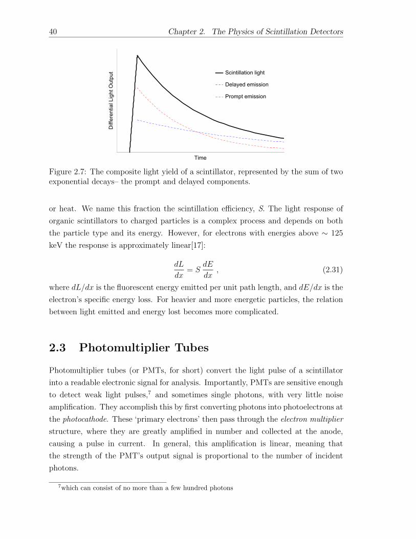
40 Chapter 2. The Physics of Scintillation Detectors
Scintillation light
Delayed emission
Prompt emission
Time
Diffe
ren
tia
lL
igh
tO
utp
ut
Figure 2.7: The composite light yield of a scintillator, represented by the sum of twoexponential decays– the prompt and delayed components.
or heat. We name this fraction the scintillation efficiency, S. The light response of
organic scintillators to charged particles is a complex process and depends on both
the particle type and its energy. However, for electrons with energies above ∼ 125
keV the response is approximately linear[17]:
dL
dx= S
dE
dx, (2.31)
where dL/dx is the fluorescent energy emitted per unit path length, and dE/dx is the
electron’s specific energy loss. For heavier and more energetic particles, the relation
between light emitted and energy lost becomes more complicated.
2.3 Photomultiplier Tubes
Photomultiplier tubes (or PMTs, for short) convert the light pulse of a scintillator
into a readable electronic signal for analysis. Importantly, PMTs are sensitive enough
to detect weak light pulses,7 and sometimes single photons, with very little noise
amplification. They accomplish this by first converting photons into photoelectrons at
the photocathode. These ‘primary electrons’ then pass through the electron multiplier
structure, where they are greatly amplified in number and collected at the anode,
causing a pulse in current. In general, this amplification is linear, meaning that
the strength of the PMT’s output signal is proportional to the number of incident
photons.
7which can consist of no more than a few hundred photons
2.3. Photomultiplier Tubes 41
Incident Photon
Photocathode
Focusing Electrode
1st Dynode
2nd Dynode Last Dynode
Anode
Photoelectron
e
Electron Multiplier
Vacuum Enclosure
Figure 2.8: Basic elements of a photomultiplier tube.
2.3.1 The Photocathode
At the photocathode, photons are converted to electrons via the photoelectric effect.
This process occurs when an incident photon is absorbed, and its energy E = hν is
transferred to an electron in the photocathode. The electron then migrates to the
surface of the photocathode, losing some of its energy to electron-electron collisions.
If the electron has sufficient energy left to overcome the material’s work function φ,
then it is emitted with kinetic energy
E < hν − φ . (2.32)
The work function φ represents the inherent potential barrier that exists at any
material-vacuum interface. It is clear that φ imposes a minimum frequency on ν, be-
low which the photoelectric effect cannot occur. Even above this threshold, however,
the photocathode is an imperfect emitter; depending on the path the electrons take,
some may lose enough energy to be unable to escape. As such, photocathodes are
delicately optimized to have a high escape depth8 while remaining (mostly) opaque
to photons; if the photocathode is too thin, it may be too transparent to photons,
despite having a relatively high efficiency for emitting photoelectrons. Evidently,
8The depth in the material at which electrons may originate and still reach the surface withsufficient energy to escape
42 Chapter 2. The Physics of Scintillation Detectors
photocathodes have an intrinsic quantum efficiency
η(λ) =# of photoelectrons emitted
# of incident photons of wavelength λ, (2.33)
which for most applications reaches its maximum at about 20-30%.
An important consequence of the photocathode’s high sensitivity (low-φ) is the
phenomenon of spontaneous electron emission. Electrons in the conduction band of
the photocathode carry some thermal kinetic energy, and, on average, this energy is
lower than φ. However, the spread of their distribution may be large enough that
electrons at the extreme high-end will have thermal kinetic energy greater than φ. If
these electrons are also near the photocathode surface, they can spontaneously escape,
propagate through the electron multiplier, and be read as a weak output signal. The
presence of these spontaneous, thermally-induced signals is called thermionic noise
or dark count. Importantly, these are ‘single-electron events’; they are the weakest
possible signals to be detected by the PMT. We will see that single-electron events
have a characteristic pulse height spectrum, due to the statistical nature of electron
multiplication and the properties of the PMT itself.
2.3.2 Electron Multplier
The electron multiplier structure consists of a chain of electrodes called dynodes.
At each dynode, a single high-energy electron is able to liberate several low-energy
electrons via secondary electron emission. In this process, electrons in the dynode
material are excited into the conduction band by the passage of an incident ener-
getic electron. Similar to the photoelectric effect in the photocathode, these excited
electrons then migrate to the surface and, if they have sufficient energy, are able to
escape the dynode.
The multiplication factor for a single dynode is defined as
δ =# of secondary electrons emitted
incident electron, (2.34)
and is generally a sensitive function of the incident electron’s energy[17]. This is
because, for incident low-energy electrons, relatively fewer material electrons will be
excited to the conduction band. Nevertheless, these excited electrons will also be
formed closer to the dynode surface, due to the low penetrative power of the primary
electron. On the other hand, incident high-energy electrons can excite more material
electrons, but at greater average depth, and thus having lower probability of escape.
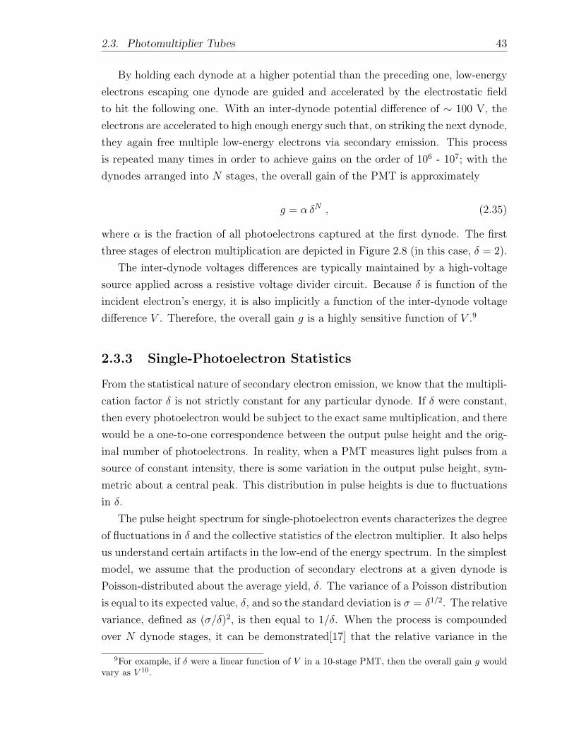
2.3. Photomultiplier Tubes 43
By holding each dynode at a higher potential than the preceding one, low-energy
electrons escaping one dynode are guided and accelerated by the electrostatic field
to hit the following one. With an inter-dynode potential difference of ∼ 100 V, the
electrons are accelerated to high enough energy such that, on striking the next dynode,
they again free multiple low-energy electrons via secondary emission. This process
is repeated many times in order to achieve gains on the order of 106 - 107; with the
dynodes arranged into N stages, the overall gain of the PMT is approximately
g = α δN , (2.35)
where α is the fraction of all photoelectrons captured at the first dynode. The first
three stages of electron multiplication are depicted in Figure 2.8 (in this case, δ = 2).
The inter-dynode voltages differences are typically maintained by a high-voltage
source applied across a resistive voltage divider circuit. Because δ is function of the
incident electron’s energy, it is also implicitly a function of the inter-dynode voltage
difference V . Therefore, the overall gain g is a highly sensitive function of V .9
2.3.3 Single-Photoelectron Statistics
From the statistical nature of secondary electron emission, we know that the multipli-
cation factor δ is not strictly constant for any particular dynode. If δ were constant,
then every photoelectron would be subject to the exact same multiplication, and there
would be a one-to-one correspondence between the output pulse height and the orig-
inal number of photoelectrons. In reality, when a PMT measures light pulses from a
source of constant intensity, there is some variation in the output pulse height, sym-
metric about a central peak. This distribution in pulse heights is due to fluctuations
in δ.
The pulse height spectrum for single-photoelectron events characterizes the degree
of fluctuations in δ and the collective statistics of the electron multiplier. It also helps
us understand certain artifacts in the low-end of the energy spectrum. In the simplest
model, we assume that the production of secondary electrons at a given dynode is
Poisson-distributed about the average yield, δ. The variance of a Poisson distribution
is equal to its expected value, δ, and so the standard deviation is σ = δ1/2. The relative
variance, defined as (σ/δ)2, is then equal to 1/δ. When the process is compounded
over N dynode stages, it can be demonstrated[17] that the relative variance in the
9For example, if δ were a linear function of V in a 10-stage PMT, then the overall gain g wouldvary as V 10.
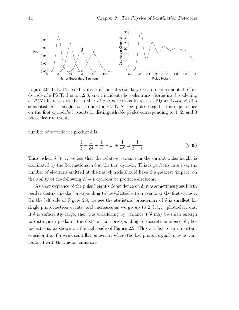
44 Chapter 2. The Physics of Scintillation Detectors
1
2
34
0 20 40 60 80 1000.00
0.02
0.04
0.06
0.08
0.10
No. of Secondary Electrons
PHNL
0.0 0.2 0.4 0.6 0.8 1.0 1.2 1.4
0
5
10
15
20
25
30
35
Pulse Height
Co
un
tsp
er
Ch
an
ne
l
Figure 2.9: Left: Probability distributions of secondary electron emission at the firstdynode of a PMT, due to 1,2,3, and 4 incident photoelectrons. Statistical broadeningof P (N) increases as the number of photoelectrons increases. Right: Low-end of asimulated pulse height spectrum of a PMT. At low pulse heights, the dependenceon the first dynode’s δ results in distinguishable peaks corresponding to 1, 2, and 3photoelectron events.
number of secondaries produced is
1
δ+
1
δ2+
1
δ3+ ... +
1
δN' 1
δ − 1. (2.36)
Thus, when δ 1, we see that the relative variance in the output pulse height is
dominated by the fluctuations in δ at the first dynode. This is perfectly intuitive; the
number of electrons emitted at the first dynode should have the greatest ‘impact’ on
the ability of the following N − 1 dynodes to produce electrons.
As a consequence of the pulse height’s dependence on δ, it is sometimes possible to
resolve distinct peaks corresponding to low-photoelectron events at the first dynode.
On the left side of Figure 2.9, we see the statistical broadening of δ is smallest for
single-photoelectron events, and increases as we go up to 2, 3, 4, ... photoelectrons.
If δ is sufficiently large, then the broadening by variance 1/δ may be small enough
to distinguish peaks in the distribution corresponding to discrete numbers of pho-
toelectrons, as shown on the right side of Figure 2.9. This artifact is an important
consideration for weak scintillation events, where the low-photon signals may be con-
founded with thermionic emissions.
Chapter 3
Detector Design and Experimental
Procedure
3.1 Apparatus
The scintillation detector used for this experiment was designed by Eljen Technology
in Sweetwater, Texas. It consists of a cylindrical (40 cm tall, 10 cm in radius) EJ-200
plastic scintillator coupled to an ETEL 9390KB photomultiplier tube via a 4-inch
thick PMMA light guide. The scintillator and light guide are both wrapped in a
light-tight black vinyl cover with an internal reflective layer for collection efficiency.
EJ-200 is a Polyvinyl-Toluene (PVT) based scintillator that is doped with An-
thracene as a primary fluor. Like most plastics, EJ-200 has very fast timing, with a
decay time of 2.1 ns. Its emission spectrum is well-matched to the 9390B’s quantum
efficiency profile. The 9390B has 10 dynodes, providing a gain of g = 7 × 10⁵ when
powered at 1000V. It has two signal outputs available: the anode, and the last dynode.
We use the signal from the last dynode, which is better for energy information.
For the purposes of the experiment, it is important that the PMT produce con-
sistently sized pulses when detecting electrons of the same energy, regardless of their
location in the scintillator. This is a challenge because, as the scintillation light is
emitted in all directions, only a fraction will travel directly to the PMT window; the
remainder is reflected internally at one or more surfaces of the scintillator before it
is collected. At each reflection, there is a chance for photons to escape, and opti-
cal attenuation becomes more likely the further the photons are made to travel. As
such, for decays occurring near the PMT, a greater fraction of the light is absorbed
directly than for decays of equal energy that occur far from the PMT. Therefore, if
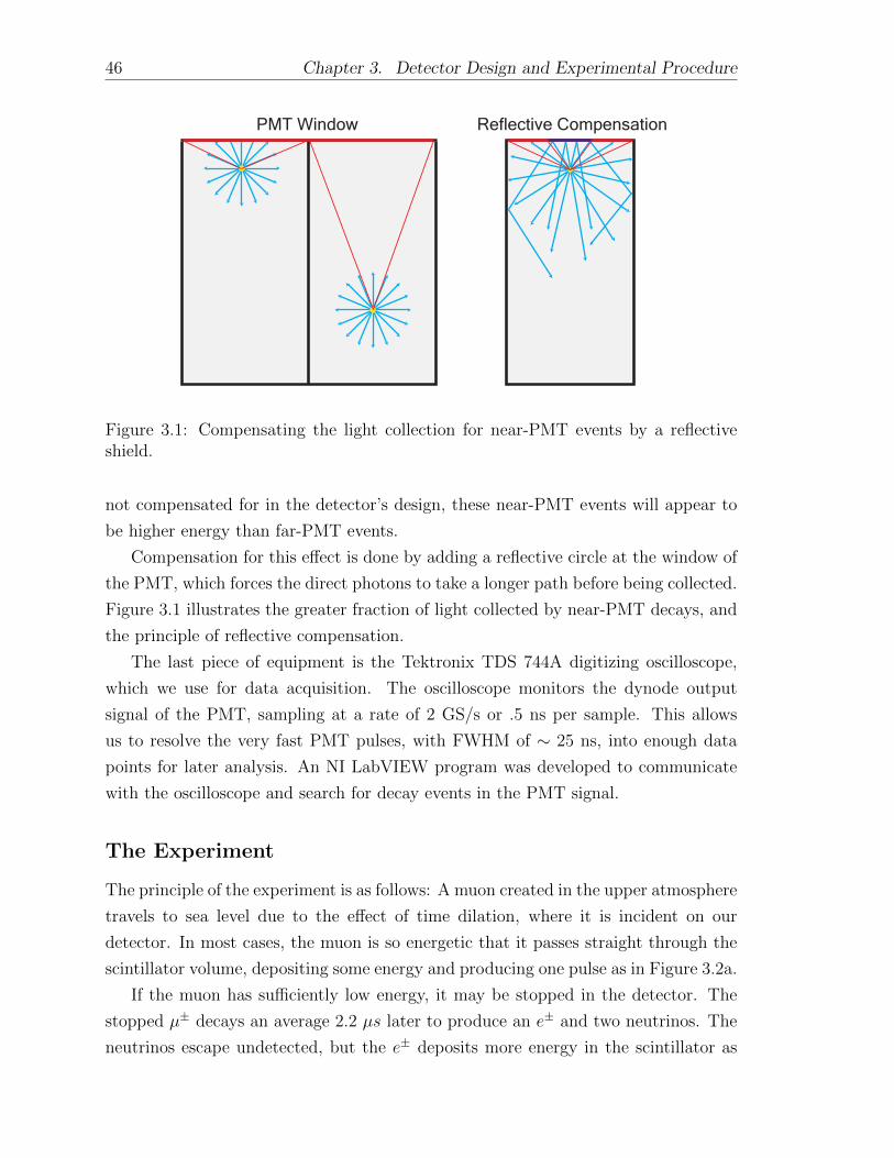
46 Chapter 3. Detector Design and Experimental Procedure
PMT Window Reflective Compensation
Figure 3.1: Compensating the light collection for near-PMT events by a reflectiveshield.
not compensated for in the detector’s design, these near-PMT events will appear to
be higher energy than far-PMT events.
Compensation for this effect is done by adding a reflective circle at the window of
the PMT, which forces the direct photons to take a longer path before being collected.
Figure 3.1 illustrates the greater fraction of light collected by near-PMT decays, and
the principle of reflective compensation.
The last piece of equipment is the Tektronix TDS 744A digitizing oscilloscope,
which we use for data acquisition. The oscilloscope monitors the dynode output
signal of the PMT, sampling at a rate of 2 GS/s or .5 ns per sample. This allows
us to resolve the very fast PMT pulses, with FWHM of ∼ 25 ns, into enough data
points for later analysis. An NI LabVIEW program was developed to communicate
with the oscilloscope and search for decay events in the PMT signal.
The Experiment
The principle of the experiment is as follows: A muon created in the upper atmosphere
travels to sea level due to the effect of time dilation, where it is incident on our
detector. In most cases, the muon is so energetic that it passes straight through the
scintillator volume, depositing some energy and producing one pulse as in Figure 3.2a.
If the muon has sufficiently low energy, it may be stopped in the detector. The
stopped µ± decays an average 2.2 µs later to produce an e± and two neutrinos. The
neutrinos escape undetected, but the e± deposits more energy in the scintillator as
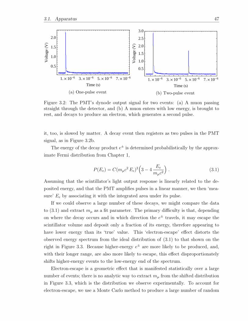
3.1. Apparatus 47
1. ´ 10-6 3. ´ 10-6 5. ´ 10-6 7. ´ 10-6
0.5
1.0
1.5
2.0
Time HsL
Volt
age
HVL
(a) One-pulse event
1. ´ 10-6 3. ´ 10-6 5. ´ 10-6 7. ´ 10-6
0.5
1.0
1.5
2.0
2.5
3.0
Time HsL
Volt
age
HVL
(b) Two-pulse event
Figure 3.2: The PMT’s dynode output signal for two events: (a) A muon passingstraight through the detector, and (b) A muon enters with low energy, is brought torest, and decays to produce an electron, which generates a second pulse.
it, too, is slowed by matter. A decay event then registers as two pulses in the PMT
signal, as in Figure 3.2b.
The energy of the decay product e± is determined probabilistically by the approx-
imate Fermi distribution from Chapter 1,
P (Ee) = C(mµc2Ee)
2(
3− 4Eemµc2
). (3.1)
Assuming that the scintillator’s light output response is linearly related to the de-
posited energy, and that the PMT amplifies pulses in a linear manner, we then ‘mea-
sure’ Ee by associating it with the integrated area under its pulse.
If we could observe a large number of these decays, we might compare the data
to (3.1) and extract mµ as a fit parameter. The primary difficulty is that, depending
on where the decay occurs and in which direction the e± travels, it may escape the
scintillator volume and deposit only a fraction of its energy, therefore appearing to
have lower energy than its ‘true’ value. This ‘electron-escape’ effect distorts the
observed energy spectrum from the ideal distribution of (3.1) to that shown on the
right in Figure 3.3. Because higher-energy e± are more likely to be produced, and,
with their longer range, are also more likely to escape, this effect disproportionately
shifts higher-energy events to the low-energy end of the spectrum.
Electron-escape is a geometric effect that is manifested statistically over a large
number of events; there is no analytic way to extract mµ from the shifted distribution
in Figure 3.3, which is the distribution we observe experimentally. To account for
electron-escape, we use a Monte Carlo method to produce a large number of random
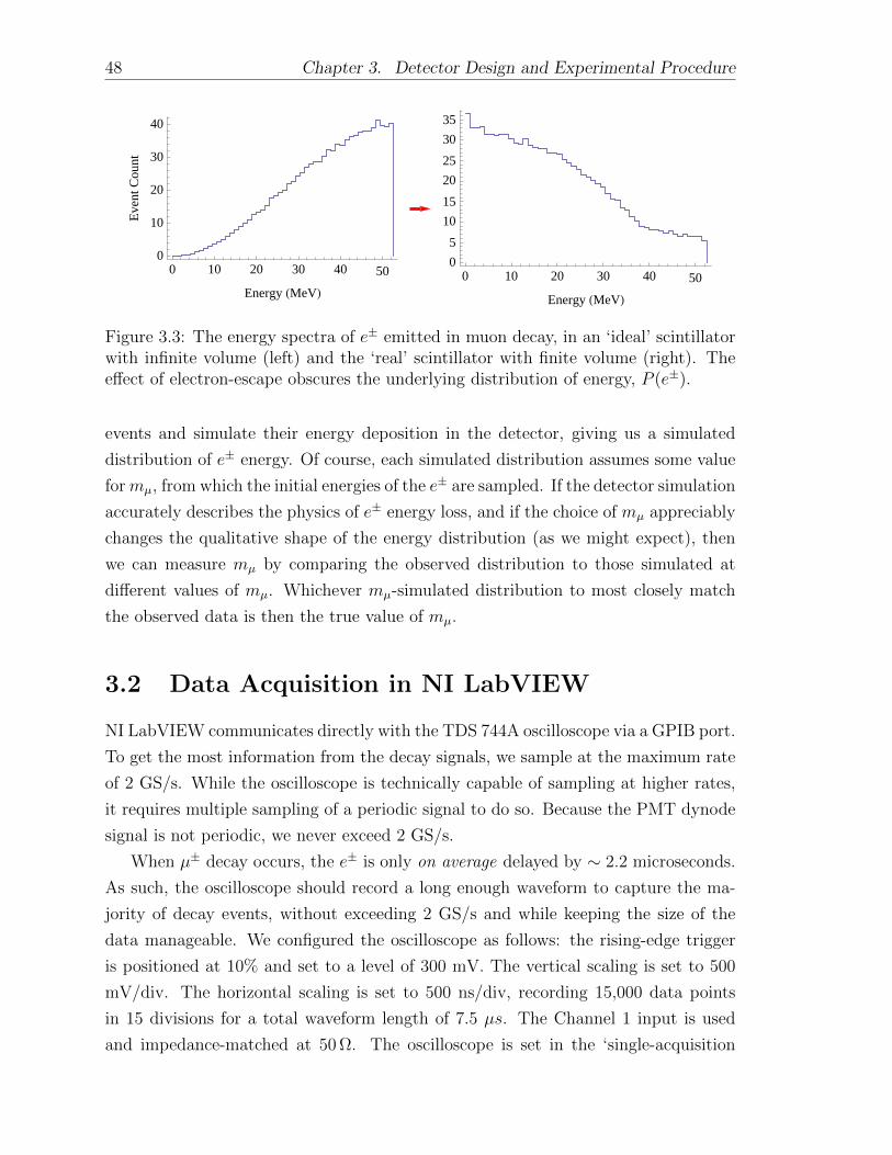
48 Chapter 3. Detector Design and Experimental Procedure
0 10 20 30 40 50
0
10
20
30
40
Energy HMeVL
Even
tC
ount
0 10 20 30 40 50
0
5
10
15
20
25
30
35
Energy HMeVL
Figure 3.3: The energy spectra of e± emitted in muon decay, in an ‘ideal’ scintillatorwith infinite volume (left) and the ‘real’ scintillator with finite volume (right). Theeffect of electron-escape obscures the underlying distribution of energy, P (e±).
events and simulate their energy deposition in the detector, giving us a simulated
distribution of e± energy. Of course, each simulated distribution assumes some value
formµ, from which the initial energies of the e± are sampled. If the detector simulation
accurately describes the physics of e± energy loss, and if the choice of mµ appreciably
changes the qualitative shape of the energy distribution (as we might expect), then
we can measure mµ by comparing the observed distribution to those simulated at
different values of mµ. Whichever mµ-simulated distribution to most closely match
the observed data is then the true value of mµ.
3.2 Data Acquisition in NI LabVIEW
NI LabVIEW communicates directly with the TDS 744A oscilloscope via a GPIB port.
To get the most information from the decay signals, we sample at the maximum rate
of 2 GS/s. While the oscilloscope is technically capable of sampling at higher rates,
it requires multiple sampling of a periodic signal to do so. Because the PMT dynode
signal is not periodic, we never exceed 2 GS/s.
When µ± decay occurs, the e± is only on average delayed by ∼ 2.2 microseconds.
As such, the oscilloscope should record a long enough waveform to capture the ma-
jority of decay events, without exceeding 2 GS/s and while keeping the size of the
data manageable. We configured the oscilloscope as follows: the rising-edge trigger
is positioned at 10% and set to a level of 300 mV. The vertical scaling is set to 500
mV/div. The horizontal scaling is set to 500 ns/div, recording 15,000 data points
in 15 divisions for a total waveform length of 7.5 µs. The Channel 1 input is used
and impedance-matched at 50 Ω. The oscilloscope is set in the ‘single-acquisition
3.3. Monte Carlo Method 49
mode’; whenever the trigger level is exceeded, the oscilloscope acquires the 15,000
point waveform record and stops sampling.
The LabVIEW program queries the oscilloscope on its acquisition state. If a
waveform is acquired, it scans the record to determine the number of pulses; if it is
not acquired, it simply waits another set period of time (1-2 seconds) before asking
again.
The number of pulses is determined by specifying a scan interval ‘s’ (in nanosec-
onds) and some sensitivity threshold, ‘n’ (an integer). The program begins by cal-
culating the mean m and standard deviation σ over the set of data points beginning
with the very first data point, and with length equal to s. Thus, if s = 500 ns, and
we are sampling at 2 GS/s, it calculates m,σ over the first 1000 data points. If the
last data point in this interval is not greater than m+ nσ, it shifts over by one point
and repeats the calculation. When some point at the end of s exceeds the threshold
m+ nσ, it is identified as a ‘candidate point’. We used n = 5 and s = 500 ns, which
prevents most of the voltage fluctuations from being read as candidates.
To prevent the scan from identifying every point on the rising edge of a pulse as
a candidate, the program skips forward by a specified interval k immediately after a
candidate is detected, and the process resumes until the scan interval reaches the end
of the waveform record. We used k = 300 ns.
If one candidate is detected, the program saves only the peak voltage of that pulse.
If two candidates are found, it saves the entire waveform record, along with a 12-value
preamble with relevant information.
3.3 Monte Carlo Method
Simulating the behavior of electrons and positrons is much more difficult than for
heavier particles; because of their small mass, e± are subject to more violent inter-
actions and frequent changes in direction. An accurate simulation must keep track
of the particle’s location as it moves through the detector, losing energy to a num-
ber of interactions. For our purpose, it is impractical to model every interaction, as
the large number of total interactions over macroscopic lengths would require enor-
mous computing power. Instead, we impose a cutoff energy above which the energy
loss processes are sampled discretely, and below which energy loss is simulated as a
continuous process.
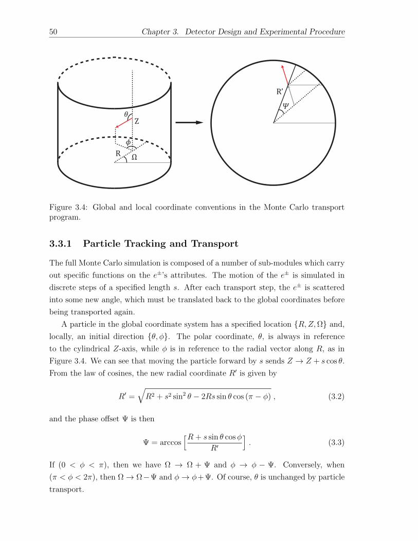
50 Chapter 3. Detector Design and Experimental Procedure
ΩR
Z𝜃
𝜙
𝛹
R’
Figure 3.4: Global and local coordinate conventions in the Monte Carlo transportprogram.
3.3.1 Particle Tracking and Transport
The full Monte Carlo simulation is composed of a number of sub-modules which carry
out specific functions on the e±’s attributes. The motion of the e± is simulated in
discrete steps of a specified length s. After each transport step, the e± is scattered
into some new angle, which must be translated back to the global coordinates before
being transported again.
A particle in the global coordinate system has a specified location R,Z,Ω and,
locally, an initial direction θ, φ. The polar coordinate, θ, is always in reference
to the cylindrical Z-axis, while φ is in reference to the radial vector along R, as in
Figure 3.4. We can see that moving the particle forward by s sends Z → Z + s cos θ.
From the law of cosines, the new radial coordinate R′ is given by
R′ =√R2 + s2 sin2 θ − 2Rs sin θ cos (π − φ) , (3.2)
and the phase offset Ψ is then
Ψ = arccos[R + s sin θ cosφ
R′
]. (3.3)
If (0 < φ < π), then we have Ω → Ω + Ψ and φ → φ − Ψ. Conversely, when
(π < φ < 2π), then Ω→ Ω−Ψ and φ→ φ+Ψ. Of course, θ is unchanged by particle
transport.
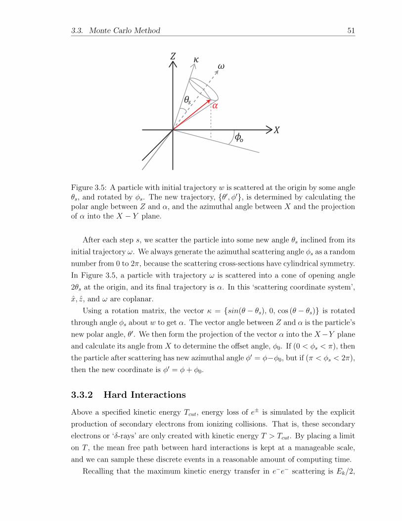
3.3. Monte Carlo Method 51
Z
X
Figure 3.5: A particle with initial trajectory w is scattered at the origin by some angleθs, and rotated by φs. The new trajectory, θ′, φ′, is determined by calculating thepolar angle between Z and α, and the azimuthal angle between X and the projectionof α into the X − Y plane.
After each step s, we scatter the particle into some new angle θs inclined from its
initial trajectory ω. We always generate the azimuthal scattering angle φs as a random
number from 0 to 2π, because the scattering cross-sections have cylindrical symmetry.
In Figure 3.5, a particle with trajectory ω is scattered into a cone of opening angle
2θs at the origin, and its final trajectory is α. In this ‘scattering coordinate system’,
x, z, and ω are coplanar.
Using a rotation matrix, the vector κ = sin(θ − θs), 0, cos (θ − θs) is rotated
through angle φs about w to get α. The vector angle between Z and α is the particle’s
new polar angle, θ′. We then form the projection of the vector α into the X−Y plane
and calculate its angle from X to determine the offset angle, φ0. If (0 < φs < π), then
the particle after scattering has new azimuthal angle φ′ = φ−φ0, but if (π < φs < 2π),
then the new coordinate is φ′ = φ+ φ0.
3.3.2 Hard Interactions
Above a specified kinetic energy Tcut, energy loss of e± is simulated by the explicit
production of secondary electrons from ionizing collisions. That is, these secondary
electrons or ‘δ-rays’ are only created with kinetic energy T > Tcut. By placing a limit
on T , the mean free path between hard interactions is kept at a manageable scale,
and we can sample these discrete events in a reasonable amount of computing time.
Recalling that the maximum kinetic energy transfer in e−e− scattering is Ek/2,
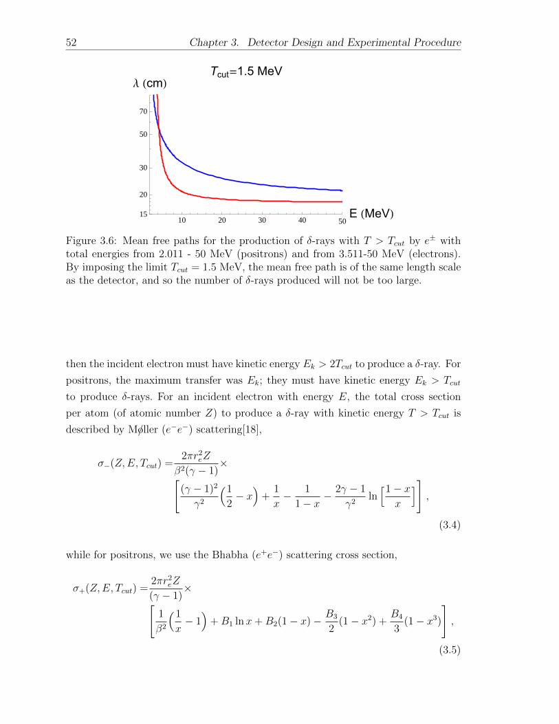
52 Chapter 3. Detector Design and Experimental Procedure
10 20 30 40 50E HMeVL
50
20
30
15
70
Λ HcmLTcut=1.5 MeV
Figure 3.6: Mean free paths for the production of δ-rays with T > Tcut by e± withtotal energies from 2.011 - 50 MeV (positrons) and from 3.511-50 MeV (electrons).By imposing the limit Tcut = 1.5 MeV, the mean free path is of the same length scaleas the detector, and so the number of δ-rays produced will not be too large.
then the incident electron must have kinetic energy Ek > 2Tcut to produce a δ-ray. For
positrons, the maximum transfer was Ek; they must have kinetic energy Ek > Tcut
to produce δ-rays. For an incident electron with energy E, the total cross section
per atom (of atomic number Z) to produce a δ-ray with kinetic energy T > Tcut is
described by M/oller (e−e−) scattering[18],
σ−(Z,E, Tcut) =2πr2
eZ
β2(γ − 1)×[
(γ − 1)2
γ2
(1
2− x)
+1
x− 1
1− x− 2γ − 1
γ2ln[1− x
x
]],
(3.4)
while for positrons, we use the Bhabha (e+e−) scattering cross section,
σ+(Z,E, Tcut) =2πr2
eZ
(γ − 1)×[
1
β2
(1
x− 1)
+B1 lnx+B2(1− x)− B3
2(1− x2) +
B4
3(1− x3)
],
(3.5)
3.3. Monte Carlo Method 53
with classical electron radius re, electron rest mass energy me, and
β = v/c γ =E/me
x =Tcut/(E −me) y = 1/(γ + 1)
B1 = 2− y2 B2 = (1− 2y)(3 + y2)
B3 = (1− 2y)2 + (1− 2y)3 B4 = (1− 2y)3 .
In our scintillator, the density of Hydrogen atoms is NH = 5.17× 10²² atoms per
cm3, and the density of Carbon atoms is NC = 4.69×10²² atoms per cm3. Therefore,
the mean free path for these hard collisions is calculated by
λ±(E, Tcut) =
(∑i
[Ni × σ±(Zi, E, Tcut)
])−1
. (3.6)
The kinetic energy T of the produced δ-ray is sampled from the differential cross
sections per atom for M/oller and Bhabha scattering. With ε = T/(E−me), where E
is the energy of the incident electron, we have
dσ
dε(Z,E, T ) =
2πr2eZ
β2(γ − 1)×[
(γ − 1)2
γ2+
1
ε
(1
ε− 2γ − 1
γ2
)+
1
1− ε
( 1
1− ε− 2γ − 1
γ2
)],
(3.7)
and for an incident positron, we have
dσ
dε(Z,E, T ) =
2πr2eZ
(γ − 1)
[1
β2ε2− B1
ε+B2 −B3ε+B4ε
2
]. (3.8)
As a practical matter, we first integrate the differential cross sections over the accord-
ing kinematic limits (Tcut ≤ T ≤ Ek/2 for e−e−, or Tcut ≤ T ≤ Ek for e+e−) to get a
normalization factor, N . Then, a value of T is sampled as a random variate from the
normalized probability distribution
P (T ) =1
N
(NH
dσ
dε(1, E, T ) +NC
dσ
dε(6, E, T )
). (3.9)
The initial particle is left with kinetic energy Ek − T . From conservation of
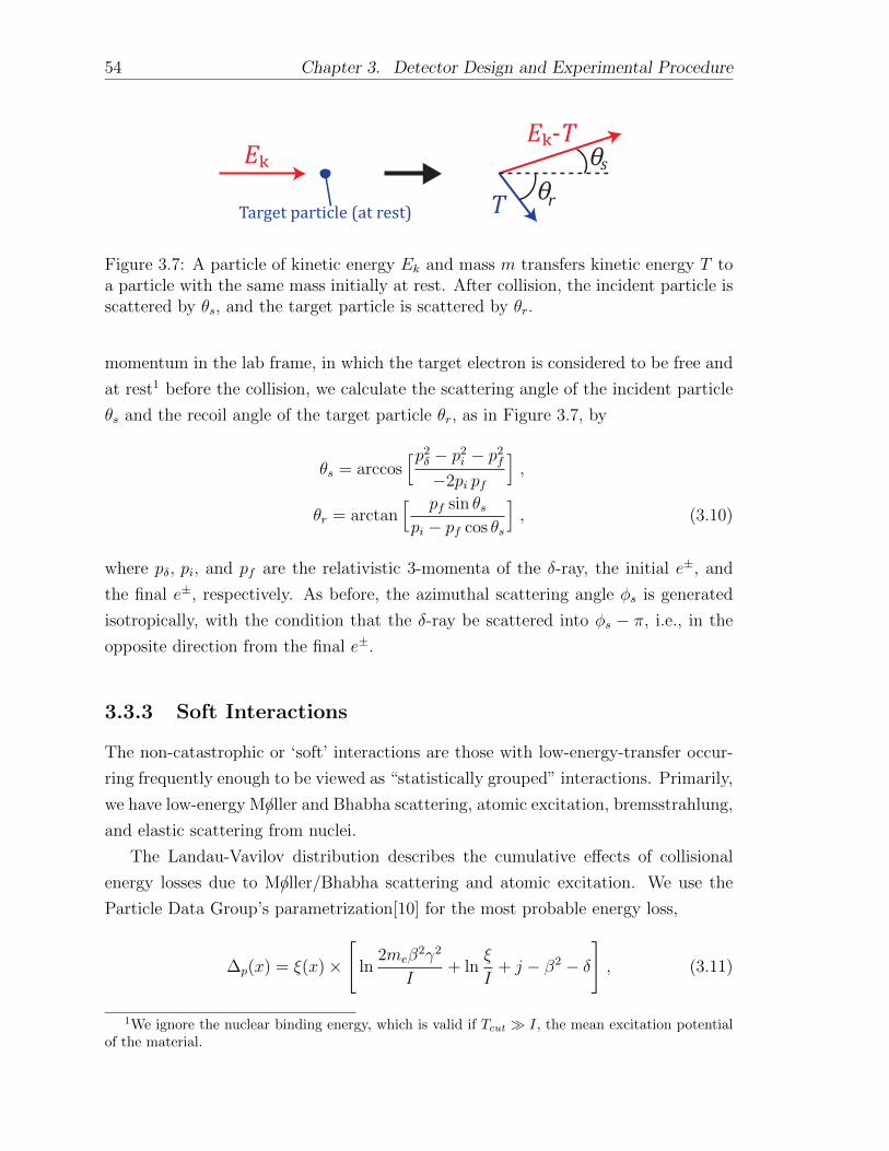
54 Chapter 3. Detector Design and Experimental Procedure
EE-T
T θθs
rTarget particle (at rest)
Figure 3.7: A particle of kinetic energy Ek and mass m transfers kinetic energy T toa particle with the same mass initially at rest. After collision, the incident particle isscattered by θs, and the target particle is scattered by θr.
momentum in the lab frame, in which the target electron is considered to be free and
at rest1 before the collision, we calculate the scattering angle of the incident particle
θs and the recoil angle of the target particle θr, as in Figure 3.7, by
θs = arccos[p2
δ − p2i − p2
f
−2pi pf
],
θr = arctan[ pf sin θspi − pf cos θs
], (3.10)
where pδ, pi, and pf are the relativistic 3-momenta of the δ-ray, the initial e±, and
the final e±, respectively. As before, the azimuthal scattering angle φs is generated
isotropically, with the condition that the δ-ray be scattered into φs − π, i.e., in the
opposite direction from the final e±.
3.3.3 Soft Interactions
The non-catastrophic or ‘soft’ interactions are those with low-energy-transfer occur-
ring frequently enough to be viewed as “statistically grouped” interactions. Primarily,
we have low-energy M/oller and Bhabha scattering, atomic excitation, bremsstrahlung,
and elastic scattering from nuclei.
The Landau-Vavilov distribution describes the cumulative effects of collisional
energy losses due to M/oller/Bhabha scattering and atomic excitation. We use the
Particle Data Group’s parametrization[10] for the most probable energy loss,
∆p(x) = ξ(x)×
[ln
2meβ2γ2
I+ ln
ξ
I+ j − β2 − δ
], (3.11)
1We ignore the nuclear binding energy, which is valid if Tcut I, the mean excitation potentialof the material.
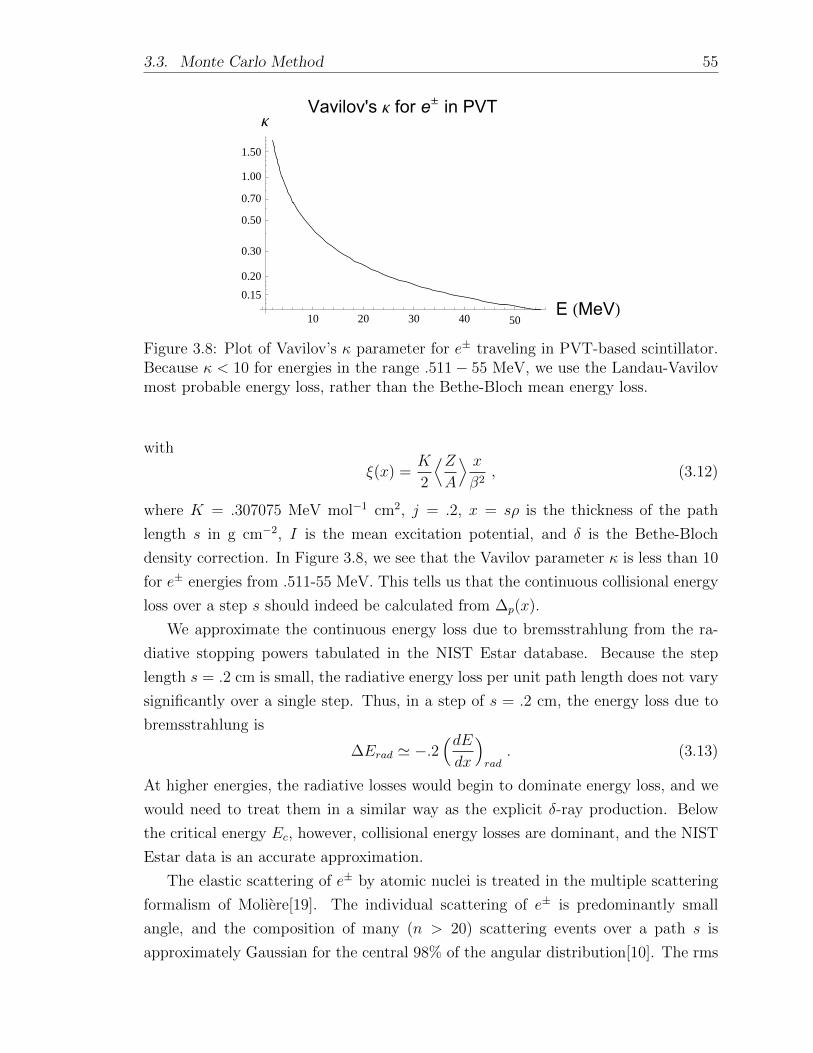
3.3. Monte Carlo Method 55
10 20 30 40 50E HMeVL
1.00
0.50
0.20
0.30
0.15
1.50
0.70
ΚVavilov's Κ for e
± in PVT
Figure 3.8: Plot of Vavilov’s κ parameter for e± traveling in PVT-based scintillator.Because κ < 10 for energies in the range .511− 55 MeV, we use the Landau-Vavilovmost probable energy loss, rather than the Bethe-Bloch mean energy loss.
with
ξ(x) =K
2
⟨ZA
⟩ xβ2
, (3.12)
where K = .307075 MeV mol−1 cm2, j = .2, x = sρ is the thickness of the path
length s in g cm−2, I is the mean excitation potential, and δ is the Bethe-Bloch
density correction. In Figure 3.8, we see that the Vavilov parameter κ is less than 10
for e± energies from .511-55 MeV. This tells us that the continuous collisional energy
loss over a step s should indeed be calculated from ∆p(x).
We approximate the continuous energy loss due to bremsstrahlung from the ra-
diative stopping powers tabulated in the NIST Estar database. Because the step
length s = .2 cm is small, the radiative energy loss per unit path length does not vary
significantly over a single step. Thus, in a step of s = .2 cm, the energy loss due to
bremsstrahlung is
∆Erad ' −.2(dEdx
)rad
. (3.13)
At higher energies, the radiative losses would begin to dominate energy loss, and we
would need to treat them in a similar way as the explicit δ-ray production. Below
the critical energy Ec, however, collisional energy losses are dominant, and the NIST
Estar data is an accurate approximation.
The elastic scattering of e± by atomic nuclei is treated in the multiple scattering
formalism of Moliere[19]. The individual scattering of e± is predominantly small
angle, and the composition of many (n > 20) scattering events over a path s is
approximately Gaussian for the central 98% of the angular distribution[10]. The rms
56 Chapter 3. Detector Design and Experimental Procedure
angular deflection, after traveling s cm, is given by
θrms =13.6 MeV
v p
√s/X0
[1 + .038 ln(s/X0)
], (3.14)
where v and p are the velocity and momentum of the incident e±, and X0 is the
radiation length in PVT, 42.54 cm.
3.3.4 Simulation Logic
The full simulation takes five inputs: number of events Nsim, muon rest energy mµ,
energy cutoff Ecut, production threshold Tcut, and step length s. An event is generated
by randomly assigning a location R,Z with R < 10 cm and Z < 40 cm, a charge
C = 1 or −1, and an energy me < Ee < (m2µ +m2
e)/2mµ.
The trajectory θ, φ is sampled by generating three random numbers X, Y, Z,
each from the interval [−1, 1]. If R =√X2 + Y 2 + Z2 ≤ 1, then θ is taken to be
the polar angle of the vector X, Y, Z in spherical coordinates, and φ is the angle
between the projection X, Y, 0 and the X-axis, running from 0 to 2π.
We name variables L = 0, Ek = Ee − me, and Ed = 0 to keep track of the
particle’s traveled distance, remaining kinetic energy, and total deposited energy in
the detector. At the beginning of the simulation and after each transport step, we
check if Ek > Ecut. If Ek < Ecut, then the particle is ‘terminated’, and we set its
kinetic energy to Ek = 0 while Ed → Ed + Ek; it deposits all of its remaining kinetic
energy to the detector.
If we have Ek > Ecut to begin with, then the program calculates λ±(Ek+me, Tcut),
the distance e± must travel before a hard collision occurs. We transport the particle
from R,Z,Ω → R′, Z ′,Ω′ by step length s, and if R′ < 10 and 0 < Z ′ < 40,
we then calculate the collisional and radiative energy losses from (3.11) and (3.13),
subtract them from Ek, and add them to Ed. We set L → L + s and calculate the
deflection angle θrms due to multiple elastic scattering from nuclei from (3.14). The
particle’s trajectory is then transformed from θ, φ → θ′, φ′ using the geometric
procedure outlined earlier, and we are ready to repeat the transport procedure.
If a transport step takes a particle outside of the detector boundary, i.e. R′ > 10,
Z ′ < 0, or Z ′ > 40, then we calculate its energy loss over a distance s/2, add this to
Ed, and terminate the particle’s history by setting Ek = 0.
Whenever the traveled distance L exceeds λ±, we generate a secondary electron by
sampling its kinetic energy T as previously described. The primary particle’s kinetic
energy is then set to Ek → Ek − T , and the path length to the next hard collision is
3.3. Monte Carlo Method 57
re-calculated at energy Ek − T +me, while L is set to 0. No change is made to Ed.
The scattering angles of the primary and secondary particles, θs and θr, are cal-
culated by (3.10) and their trajectories are transformed to θ′, φ′. The location,
trajectory, and kinetic energy of the secondary particle is saved, and the primary
particle continues to be transported and transformed until it either deposits all of its
kinetic energy or escapes the detector. Each secondary particle is then transported
and transformed just as if it were a primary particle, and the total energy deposition
is then Ed = Epd +E1
d +E2d +...+En
d , where n is the number of secondary particles cre-
ated by the primary, p. As a last step, we simulate positron annihilation e+e− → γ γ
by adding 2me to Ed whenever a positron reaches Ek < Ecut, in addition to whatever
residual kinetic energy it deposits in the detector.
In Figure 3.9, we see that the electrons traveling through matter follow a tortuous
path as they lose energy to soft collisions, bremsstrahlung, and the generation of δ-
rays. We can imagine, then, that high-energy e± produced in muon decays should be
even more susceptible to electron escape, as they produce more secondary particles
and are deflected from their path more often than low-energy e±, providing more
instances for energy be carried out of the detector.
Every event has a ‘true’ energy Ee that we sampled randomly, and an ‘apparent’
or deposited energy, Ed. After calculating Ed, we assign each event a ‘probability
factor’ of Q = R × P (Ee), where P (Ee) is the probability that an e± be produced
with energy Ee in µ± decay, from Chapter 1. R is simply the initial radial coordinate,
which is applied to account for the fact that the differential volume within the detector
at radius R scales by a factor of R. The probability factor Q is where we recover
the underlying physics of muon decay, by preferentially weighting events in the high-
energy end of the spectrum as predicted by the Fermi distribution.
An energy distribution is formed from a large set of Ed, Q events. Because the
simulated and experimental data use different metrics for measuring Ee, all distribu-
tions are normalized to their highest energy value; for a set of simulated events, each
Eid is divided by the maximum Emax
d of the set. We specify a binning number, n, and
group events into evenly-spaced increments of width 1/n. The Q factors are summed
in each bin, and finally, we normalize the sum of all Q’s to equal the number of data
points in the experimental distribution.
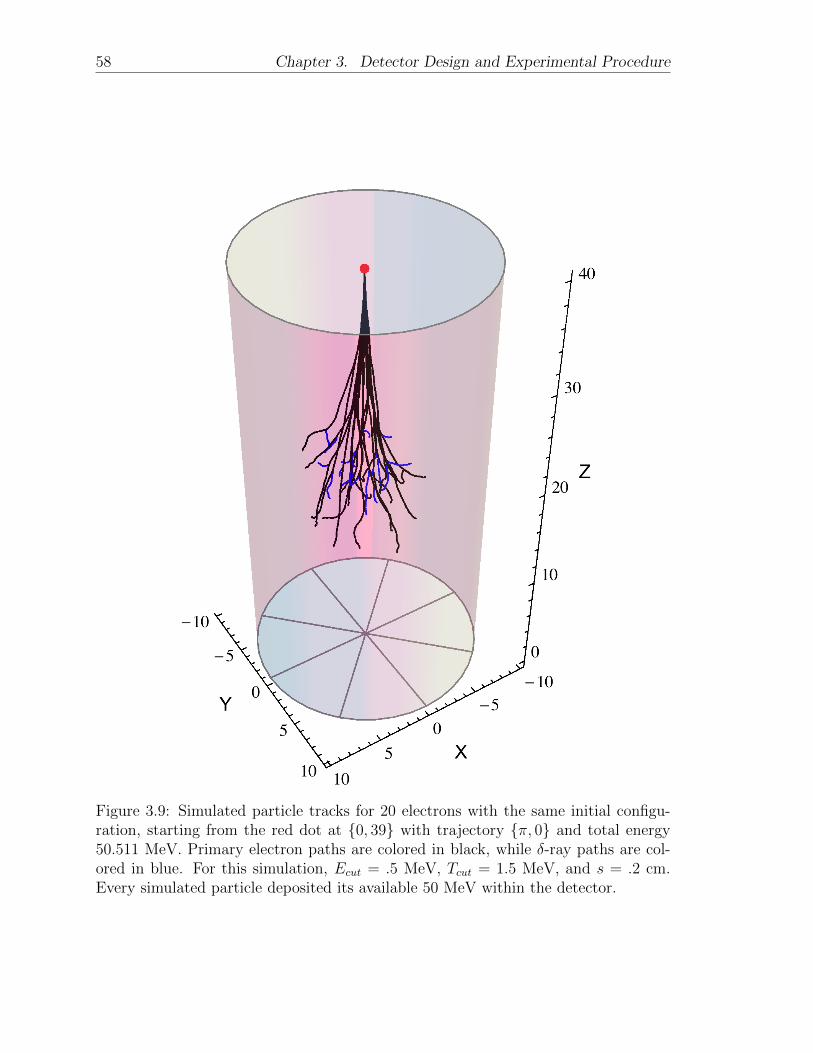
58 Chapter 3. Detector Design and Experimental Procedure
Figure 3.9: Simulated particle tracks for 20 electrons with the same initial configu-ration, starting from the red dot at 0, 39 with trajectory π, 0 and total energy50.511 MeV. Primary electron paths are colored in black, while δ-ray paths are col-ored in blue. For this simulation, Ecut = .5 MeV, Tcut = 1.5 MeV, and s = .2 cm.Every simulated particle deposited its available 50 MeV within the detector.
Chapter 4
Results and Analysis
Data were collected daily from 2/12/2015 to 4/15/2015 with the PMT powered at
1200 V and 1000 V for roughly equal periods of collection time. At 1200 V, one-
pulse events were only recorded after 2/28/2015, with a total 565620 one-pulse events
recorded. In the same period of time, 4163 two-pulse events were recorded. Therefore,
approximately one event in 137 is a two-pulse event. In total, 6309 two-pulse events
were recorded at 1200 V, and 4303 two-pulse events were recorded at 1000 V. We also
recorded 628124 one-pulse events at 1000 V.
All events were recorded with the same configurations as detailed in Chapter 3,
except for the difference in supplied voltage of the PMT. Each two-pulse data record
is structured as
Np, dt, Vpk, ipk, ∆t, m1, σ1, m2, σ2, i1, i2, s, (waveform data) ,
where Np is the number of points in (waveform data), dt is the time per point, Vpk is
the peak voltage of the second pulse, ipk is the offset index of this peak from the second
candidate point, and ∆t is the time elapsed between first and second candidates. mn
and σn are the mean and standard deviation preceding the nth candidate point, and
in is its index in (waveform data). s is the scan length in number of data points.
Waveform data is simply the voltage values of each of the data points in the record.
4.1 Pulse Processing & Integration
The data must first be processed and integrated to constitute a ‘measurement’ of
Ee± . First, we throw out any events where ∆t < tcut for a specified value of tcut. We
want to avoid two-pulse events where the e± signal occurs too soon after the µ±’s,
60 Chapter 4. Results and Analysis
because the delayed component of the first signal may be ‘buried’ underneath the
second signal, thus raising it artificially. We used tcut = 1.0× 10⁻⁶ s, which appears
to be long enough for the µ± signal to decay completely. As Ee± is not correlated
with the muon lifetime τµ, removing events by ∆t < tcut does not bias the remaining
data. This step cuts 1095 events from the 1200V-data and 863 from the 1000V-data.
Next, we clip off the waveform data preceding i2, as we are only interested in the
second signal. We subtract m2 from the remaining data points in order to remove any
‘baseline’ voltage preceding the signal, as again, we are only interested in the change
in voltage due to the passage of an e± through the detector.
While the LabVIEW program finds the candidate start point, i2, we now need
to choose the ‘endpoint’ of our integration, where the second pulse has effectively
reached zero. Similar to before, we specify an integer nf , and test each point (to
the right of the peak, ipk) to see if it has fallen below nf σ2. If we reach the end of
the waveform without finding such a point, then the signal was clipped at the end of
the oscilloscope’s acquisition before it could relax to zero. These events are thrown
out from the remaining data, and the waveforms are clipped off past the determined
endpoint.
We add another stage of amplitude discrimination to remove ‘blip’ events and
very weak signals. Blips occur when a single point jumps above 5σ2 due to noise in
the PMT signal, thus registering as a second pulse. If, in the remaining waveform, no
data points exceed ncut σ2, then the event is thrown out. We used ncut = 6 to ensure
that all data points have at least some ‘rising’ and ‘falling’ shape. This cuts another
924 events from the 1200V-data and 154 events from the 1000V-data.
Finally, we generate an interpolating function for each waveform, and integrate the
area under the resulting curve in Mathematica. We normalize these ‘energies’ to the
maximum value of the set, then bin the data to produce an experimental distribution.
4.2 Energy Distributions
The experimental energy distributions are plotted in Figure 4.1. Here, χ is split into
30 bins. The two distributions differ most significantly in the low-energy regime. In
the 1200 V-data, the first two bins contain 1139 events, just over 1/4 of all plotted
events. By comparison, the 1000 V-data contains 374 events in its lowest two bins,
or ∼ 1/10 of all plotted events. This discrepancy can be understood as due to higher
inter-dynode voltage differences when the PMT is operated at 1200 V as opposed to
1000 V. We also see that a very small number of exceptionally high-energy events,
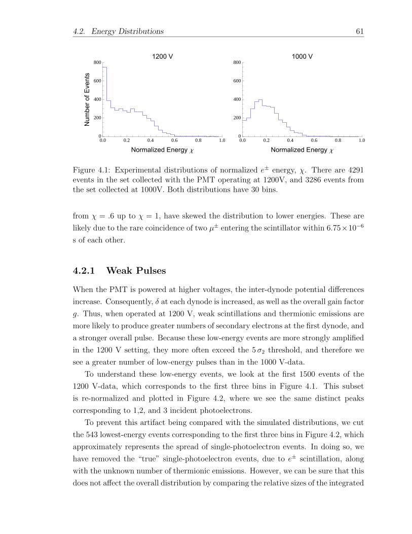
4.2. Energy Distributions 61
0.0 0.2 0.4 0.6 0.8 1.00
200
400
600
800
Normalized Energy Χ
Nu
mb
er
of
Eve
nts
1200 V
0.0 0.2 0.4 0.6 0.8 1.00
200
400
600
800
Normalized Energy Χ
1000 V
Figure 4.1: Experimental distributions of normalized e± energy, χ. There are 4291events in the set collected with the PMT operating at 1200V, and 3286 events fromthe set collected at 1000V. Both distributions have 30 bins.
from χ = .6 up to χ = 1, have skewed the distribution to lower energies. These are
likely due to the rare coincidence of two µ± entering the scintillator within 6.75×10⁻⁶
s of each other.
4.2.1 Weak Pulses
When the PMT is powered at higher voltages, the inter-dynode potential differences
increase. Consequently, δ at each dynode is increased, as well as the overall gain factor
g. Thus, when operated at 1200 V, weak scintillations and thermionic emissions are
more likely to produce greater numbers of secondary electrons at the first dynode, and
a stronger overall pulse. Because these low-energy events are more strongly amplified
in the 1200 V setting, they more often exceed the 5σ2 threshold, and therefore we
see a greater number of low-energy pulses than in the 1000 V-data.
To understand these low-energy events, we look at the first 1500 events of the
1200 V-data, which corresponds to the first three bins in Figure 4.1. This subset
is re-normalized and plotted in Figure 4.2, where we see the same distinct peaks
corresponding to 1,2, and 3 incident photoelectrons.
To prevent this artifact being compared with the simulated distributions, we cut
the 543 lowest-energy events corresponding to the first three bins in Figure 4.2, which
approximately represents the spread of single-photoelectron events. In doing so, we
have removed the “true” single-photoelectron events, due to e± scintillation, along
with the unknown number of thermionic emissions. However, we can be sure that this
does not affect the overall distribution by comparing the relative sizes of the integrated
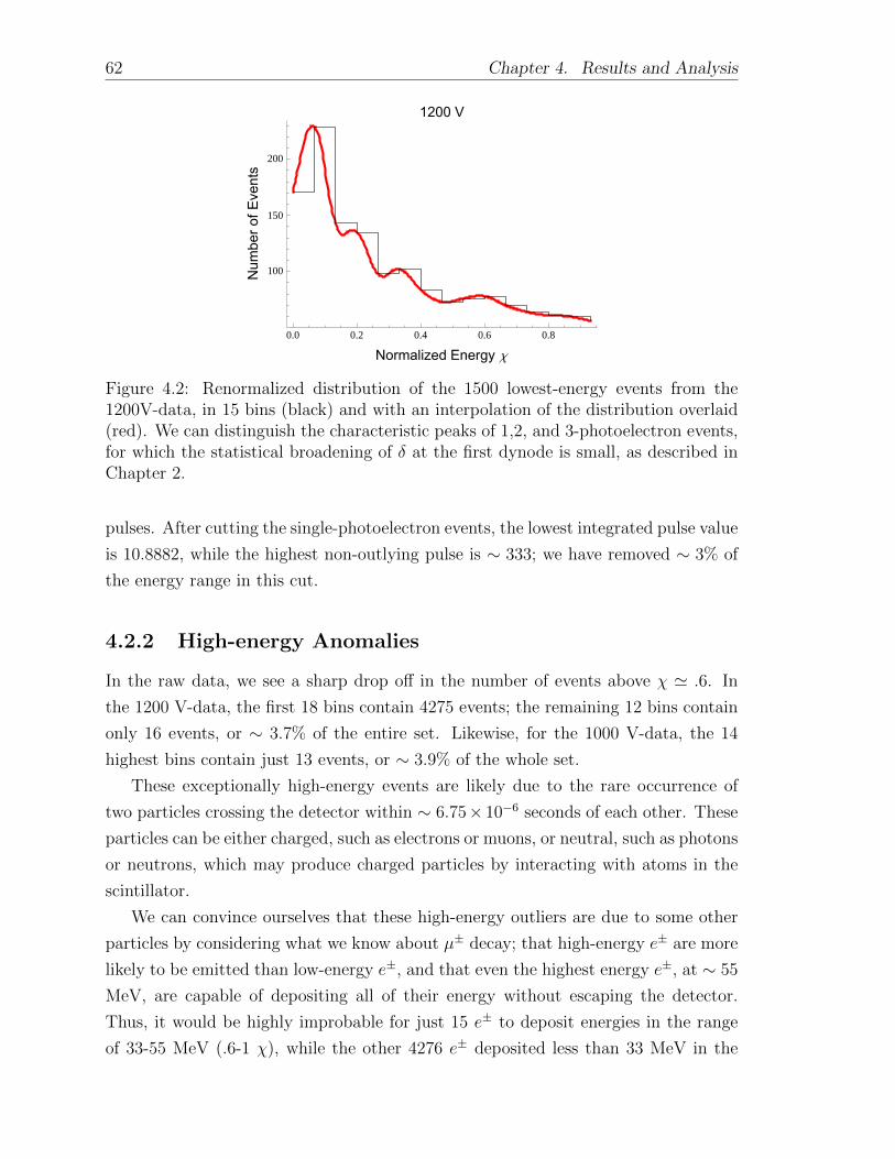
62 Chapter 4. Results and Analysis
0.0 0.2 0.4 0.6 0.8
100
150
200
Normalized Energy Χ
Nu
mb
er
of
Eve
nts
1200 V
Figure 4.2: Renormalized distribution of the 1500 lowest-energy events from the1200V-data, in 15 bins (black) and with an interpolation of the distribution overlaid(red). We can distinguish the characteristic peaks of 1,2, and 3-photoelectron events,for which the statistical broadening of δ at the first dynode is small, as described inChapter 2.
pulses. After cutting the single-photoelectron events, the lowest integrated pulse value
is 10.8882, while the highest non-outlying pulse is ∼ 333; we have removed ∼ 3% of
the energy range in this cut.
4.2.2 High-energy Anomalies
In the raw data, we see a sharp drop off in the number of events above χ ' .6. In
the 1200 V-data, the first 18 bins contain 4275 events; the remaining 12 bins contain
only 16 events, or ∼ 3.7% of the entire set. Likewise, for the 1000 V-data, the 14
highest bins contain just 13 events, or ∼ 3.9% of the whole set.
These exceptionally high-energy events are likely due to the rare occurrence of
two particles crossing the detector within ∼ 6.75× 10⁻⁶ seconds of each other. These
particles can be either charged, such as electrons or muons, or neutral, such as photons
or neutrons, which may produce charged particles by interacting with atoms in the
scintillator.
We can convince ourselves that these high-energy outliers are due to some other
particles by considering what we know about µ± decay; that high-energy e± are more
likely to be emitted than low-energy e±, and that even the highest energy e±, at ∼ 55
MeV, are capable of depositing all of their energy without escaping the detector.
Thus, it would be highly improbable for just 15 e± to deposit energies in the range
of 33-55 MeV (.6-1 χ), while the other 4276 e± deposited less than 33 MeV in the
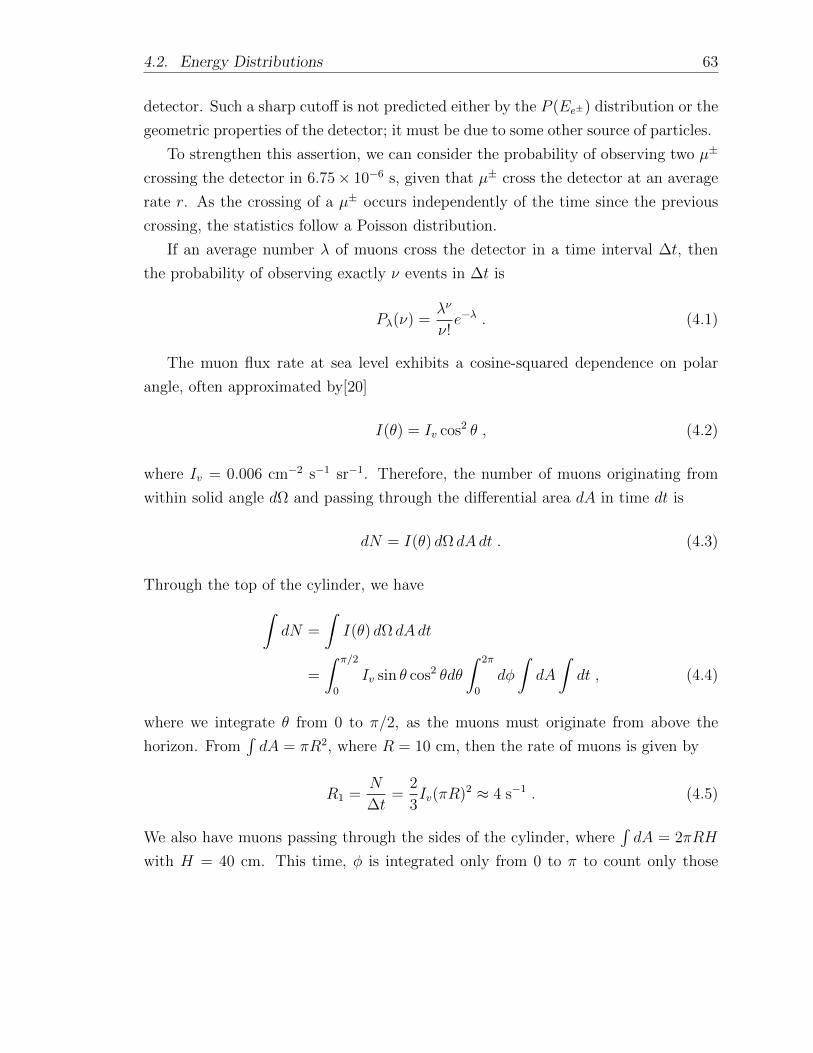
4.2. Energy Distributions 63
detector. Such a sharp cutoff is not predicted either by the P (Ee±) distribution or the
geometric properties of the detector; it must be due to some other source of particles.
To strengthen this assertion, we can consider the probability of observing two µ±
crossing the detector in 6.75× 10⁻⁶ s, given that µ± cross the detector at an average
rate r. As the crossing of a µ± occurs independently of the time since the previous
crossing, the statistics follow a Poisson distribution.
If an average number λ of muons cross the detector in a time interval ∆t, then
the probability of observing exactly ν events in ∆t is
Pλ(ν) =λν
ν!e−λ . (4.1)
The muon flux rate at sea level exhibits a cosine-squared dependence on polar
angle, often approximated by[20]
I(θ) = Iv cos2 θ , (4.2)
where Iv = 0.006 cm−2 s−1 sr−1. Therefore, the number of muons originating from
within solid angle dΩ and passing through the differential area dA in time dt is
dN = I(θ) dΩ dAdt . (4.3)
Through the top of the cylinder, we have∫dN =
∫I(θ) dΩ dAdt
=
∫ π/2
0
Iv sin θ cos2 θdθ
∫ 2π
0
dφ
∫dA
∫dt , (4.4)
where we integrate θ from 0 to π/2, as the muons must originate from above the
horizon. From∫dA = πR2, where R = 10 cm, then the rate of muons is given by
R1 =N
∆t=
2
3Iv(πR)2 ≈ 4 s−1 . (4.5)
We also have muons passing through the sides of the cylinder, where∫dA = 2πRH
with H = 40 cm. This time, φ is integrated only from 0 to π to count only those
64 Chapter 4. Results and Analysis
muons crossing into the detector from the outside:
R2 =
∫ π/2
0
sin θ cos2 θdθ
∫ π
0
dφ
∫dA
≈ 16 s−1 . (4.6)
Now, the total rate of crossing events is r ≈ 20 s−1. We are interested in the
conditional probability of observing a muon in 6.75 × 10⁻⁶ s, given that one was
observed in 7.5× 10⁻⁶ s. The conditional probability of A given B is defined as
P (A|B) =P (A ∩B)
P (B)(4.7)
where A ∩ B is the intersection of events A and B; for our problem, this is the
probability of two muons being observed in a period of 6.75× 10⁻⁶ s.
Therefore, the probability of two-muon coincidence is
Pc =(6.75 r × 10−6)2
2(7.5 r × 10−6)e r(7.5−6.75)×10−6 ≈ 6× 10⁻⁵ . (4.8)
We can now estimate how many two-pulse events were due to muon coincidence by
multiplying Pc by the total number of observations taken. At 1200 V, we observed
approximately1 864333 total events, and so we might expect to have ∼ 51 muon
coincidence events. At 1000 V, we made 632427 total observations, which would
predict ∼ 38 muon coincidence events.
While we observed 16 high-energy events in the highest 12 bins of the 1200 V-data,
there are likely additional events due to muon coincidence distributed throughout
the other 18 bins, mixed in with the µ± decay events. Thus, there may be ∼ 40
muon coincidence events in the 1200 V-data, which is near that as predicted by our
Poisson counting approximation. For the 1000 V-data, the 13 highest-energy events
were found in the highest 14 bins; by extrapolation, then, there may be ∼ 28 muon
coincidence events in all 30 bins, which again is close to the predicted value.
1Because muon data wasn’t recorded for some of the earlier runs, we estimate the number oftotal observations by multiplying the number two-pulse events, 6309, by the average ratio of totalevents to two-pulse events, 137.
4.3. Measurement of mµ 65
0 5 10 15 20 25
1 ´ 104
2 ´ 104
5 ´ 104
1 ´ 105
2 ´ 105
High-Energy Cuts
Su
mo
fS
qu
are
dR
esid
ua
ls
0.0 0.2 0.4 0.6 0.8 1.0
0
100
200
300
400
500
Normalized Energy Χ
Nu
mb
er
of
Eve
nts
Figure 4.3: Sum of squared residuals between the mµ = 105 simulated distributionand the experimental distribution with increasing cuts to the high-energy range (Left),and plots of the closest agreement between experimental and simulated distributions,when ncuts = 11 (Right). The experimental distribution is plotted in Black, and thesimulated distribution is plotted in Cyan. The simulated distribution is generatedfrom 100000 events, and normalized to the size of the experimental distribution afterhigh-range cuts.
4.3 Measurement of mµ
Having cut the 543 lowest-energy events, we must now determine the appropriate
number of cuts to the high-energy end of the 1200 V distribution. We do this by
generating a simulated distribution at mµ = 105 MeV, and comparing it to the
experimental distribution as we sequentially cut more and more high-energy events.
Specifically, the simulated and experimental distributions are binned at the same
value, and we quantify their variance by calculating the sum of the squared residuals
over all of their bins. We reduce the number of bins from 30 to 12 for a smoother
experimental distribution.
On the left side of Figure 4.3, we see that cutting the 11 highest-energy events
from the data produces the closest agreement with the simulated distribution. On the
right side, the resulting experimental distribution is plotted with that of the mµ =
105 MeV simulation. We are left with a remaining 3737 events in the experimental
distribution.
To measuremµ, we generated simulated distributions at values ofmµ = 90, 95, 100,
105, 110, 115, and 120 MeV. Each simulated distribution is generated from 100000
events, then scaled down to represent 3737 events, and the energies are normalized
to 1.
The simulated distributions are shown in comparison with the experimental dis-
tribution on the left of Figure 4.4, with the various colors representing different as-
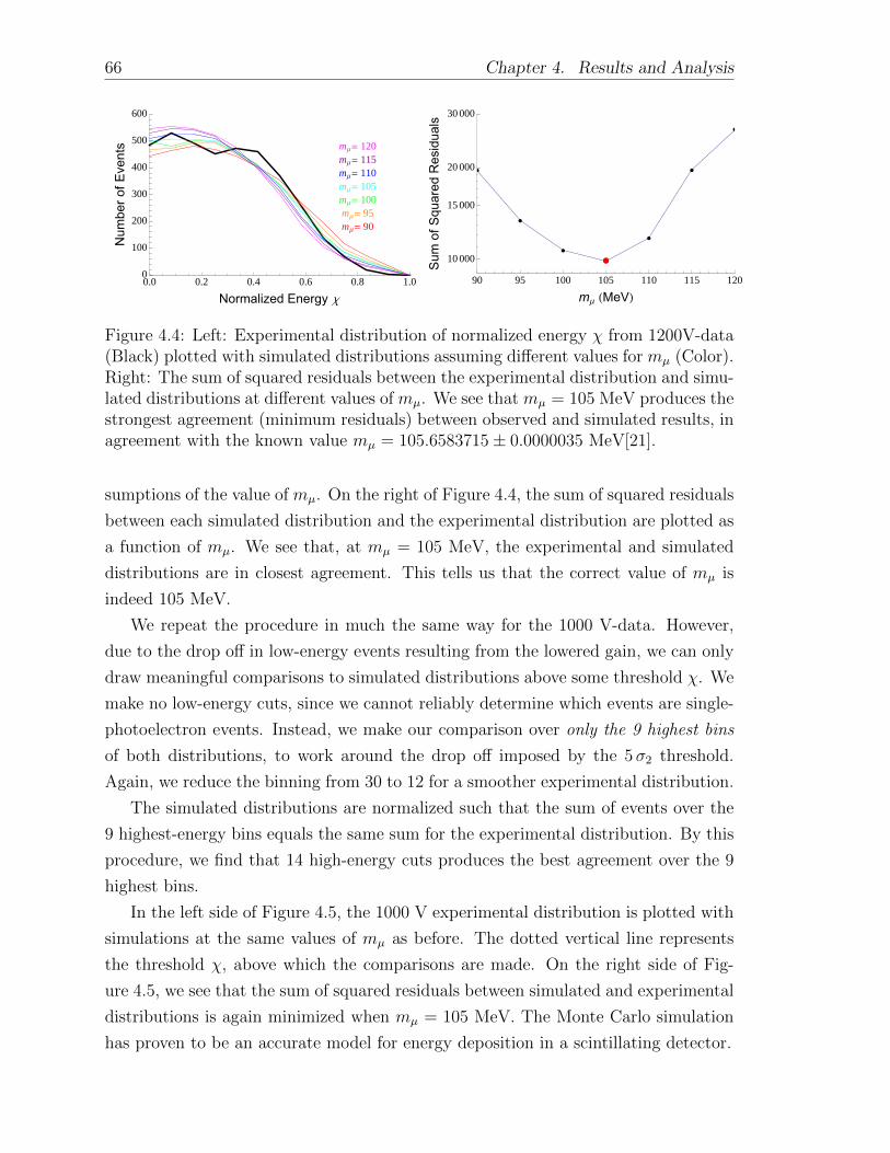
66 Chapter 4. Results and Analysis
mΜ= 90
mΜ= 95
mΜ= 100
mΜ= 105
mΜ= 110
mΜ= 115
mΜ= 120
0.0 0.2 0.4 0.6 0.8 1.00
100
200
300
400
500
600
Normalized Energy Χ
Nu
mb
er
of
Eve
nts
90 95 100 105 110 115 120
10 000
20 000
30 000
15 000
mΜ HMeVL
Su
mo
fS
qu
are
dR
esid
ua
ls
Figure 4.4: Left: Experimental distribution of normalized energy χ from 1200V-data(Black) plotted with simulated distributions assuming different values for mµ (Color).Right: The sum of squared residuals between the experimental distribution and simu-lated distributions at different values of mµ. We see that mµ = 105 MeV produces thestrongest agreement (minimum residuals) between observed and simulated results, inagreement with the known value mµ = 105.6583715± 0.0000035 MeV[21].
sumptions of the value of mµ. On the right of Figure 4.4, the sum of squared residuals
between each simulated distribution and the experimental distribution are plotted as
a function of mµ. We see that, at mµ = 105 MeV, the experimental and simulated
distributions are in closest agreement. This tells us that the correct value of mµ is
indeed 105 MeV.
We repeat the procedure in much the same way for the 1000 V-data. However,
due to the drop off in low-energy events resulting from the lowered gain, we can only
draw meaningful comparisons to simulated distributions above some threshold χ. We
make no low-energy cuts, since we cannot reliably determine which events are single-
photoelectron events. Instead, we make our comparison over only the 9 highest bins
of both distributions, to work around the drop off imposed by the 5σ2 threshold.
Again, we reduce the binning from 30 to 12 for a smoother experimental distribution.
The simulated distributions are normalized such that the sum of events over the
9 highest-energy bins equals the same sum for the experimental distribution. By this
procedure, we find that 14 high-energy cuts produces the best agreement over the 9
highest bins.
In the left side of Figure 4.5, the 1000 V experimental distribution is plotted with
simulations at the same values of mµ as before. The dotted vertical line represents
the threshold χ, above which the comparisons are made. On the right side of Fig-
ure 4.5, we see that the sum of squared residuals between simulated and experimental
distributions is again minimized when mµ = 105 MeV. The Monte Carlo simulation
has proven to be an accurate model for energy deposition in a scintillating detector.
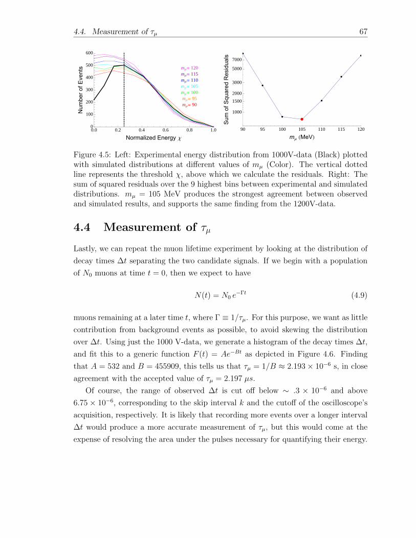
4.4. Measurement of τµ 67
mΜ= 90
mΜ= 95
mΜ= 100
mΜ= 105
mΜ= 110
mΜ= 115
mΜ= 120
0.0 0.2 0.4 0.6 0.8 1.00
100
200
300
400
500
600
Normalized Energy Χ
Nu
mb
er
of
Eve
nts
90 95 100 105 110 115 120
1000
5000
2000
3000
1500
7000
mΜ HMeVL
Su
mo
fS
qu
are
dR
esid
ua
ls
Figure 4.5: Left: Experimental energy distribution from 1000V-data (Black) plottedwith simulated distributions at different values of mµ (Color). The vertical dottedline represents the threshold χ, above which we calculate the residuals. Right: Thesum of squared residuals over the 9 highest bins between experimental and simulateddistributions. mµ = 105 MeV produces the strongest agreement between observedand simulated results, and supports the same finding from the 1200V-data.
4.4 Measurement of τµ
Lastly, we can repeat the muon lifetime experiment by looking at the distribution of
decay times ∆t separating the two candidate signals. If we begin with a population
of N0 muons at time t = 0, then we expect to have
N(t) = N0 e−Γt (4.9)
muons remaining at a later time t, where Γ ≡ 1/τµ. For this purpose, we want as little
contribution from background events as possible, to avoid skewing the distribution
over ∆t. Using just the 1000 V-data, we generate a histogram of the decay times ∆t,
and fit this to a generic function F (t) = Ae−Bt as depicted in Figure 4.6. Finding
that A = 532 and B = 455909, this tells us that τµ = 1/B ≈ 2.193× 10⁻⁶ s, in close
agreement with the accepted value of τµ = 2.197 µs.
Of course, the range of observed ∆t is cut off below ∼ .3 × 10−6 and above
6.75 × 10⁻⁶, corresponding to the skip interval k and the cutoff of the oscilloscope’s
acquisition, respectively. It is likely that recording more events over a longer interval
∆t would produce a more accurate measurement of τµ, but this would come at the
expense of resolving the area under the pulses necessary for quantifying their energy.
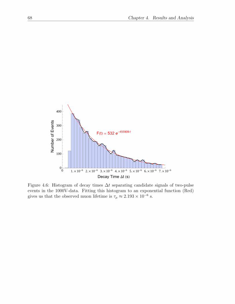
68 Chapter 4. Results and Analysis
FHtL = 532 e-455909 t
0 1. ´ 10-6
2. ´ 10-6
3. ´ 10-6
4. ´ 10-6
5. ´ 10-6
6. ´ 10-6
7. ´ 10-6
0
100
200
300
400
Decay Time Dt HsL
Nu
mb
er
of
Eve
nts
Figure 4.6: Histogram of decay times ∆t separating candidate signals of two-pulseevents in the 1000V-data. Fitting this histogram to an exponential function (Red)gives us that the observed muon lifetime is τµ ≈ 2.193× 10⁻⁶ s.
Conclusion
We began by studying the three-body decay of the muon, where we saw that the emit-
ted electron (or positron) can be produced with a range of energies, P (Ee±). Next, we
saw that the e±s deposit their energy, in the form of collisional and radiative losses,
as they traverse matter, and that this energy is rapidly converted into an electronic
signal by the scintillation detector. Assuming the amplification of scintillation pulses
to be linear, we asserted that the relative integrated areas under pulses constitutes
a measurement of the relative energies deposited by each of the e±. By observing a
large number of muon decays, we normalized the distribution of e± energies in order
to compare it with simulated distributions generated by a Monte Carlo method. We
have found that a simulated value of mµ = 105 MeV most closely matches the ob-
served distribution, and is thus the true value of mµ. We also saw that the observed
distribution of decay times exhibited the characteristic muon lifetime, τµ ≈ 2.2 µs.
The goal of this thesis was to demonstrate that large-volume scintillation detec-
tors, commonly used to measure τµ, may be adapted to measure mµ by using a fast
digitizing oscilloscope. The accuracy of this measurement may be increased on two
fronts: through collecting a larger sample of data, and through improvements to the
Monte Carlo simulation.
Although we had a limited window of operational time, we collected enough events
to claim a measurement ofmµ. With a greater number of events, we might begin to see
nuances in the shape of the experimental distributions that are not accounted for by
the simulation. Some areas of improvement would include the addition of more hard
interactions, such as large-angle single elastic scattering from nuclei, in-flight positron
annihilation, and hard bremsstrahlung emission. However, these would ultimately
necessitate a new branch of code for the transport and interaction of photons, which
is dominated at lower energies by Compton scattering. A model this complete would
require significantly longer computation times to produce simulated distributions;
our approximate model sufficiently describes the physics of energy loss by e± in a
scintillating detector.

References
[1] A discovery of cosmic proportions. CERN Courier, July 2012.
[2] J. J. Beatty, J. Matthews, and S. P. Wakely. Cosmic Rays. Particle Data Group,
October 2013.
[3] Bradley W. Carroll and Dale A. Ostlie. An Introduction to Modern Astrophysics.
Addison-Wesley, 2nd edition, 2007.
[4] Feng Xiao. Measurement of the Radiative Muon Decay Branching Fraction in
the MEG Experiment. PhD thesis, University of California, Irvine, 2010.
[5] David Griffiths. Introduction to Elementary Particles. Wiley-VCH, 2nd edition,
2008.
[6] Y. Okada Y. Kuno. Muon decay and physics beyond the standard model. Reviews
of Modern Physics, 73(1):151–202, 2001.
[7] E. A. Kuraev E. Bartox and M. Secansky. Radiative corrections to muon decay
in leading and next-to-leading approximation for electron spectrum. Physics of
Paricles and Nuclei Letters, 6(5):365–367, 2009.
[8] A. Czarnecki A. Arbuzov and A. Gaponenko. Muon decay spectrum: Leading
logarithmic approximation. Physical Review D, 65(113006), 2002.
[9] William R. Leo. Techniques for Nuclear and Particle Physics Experiments.
Springer-Verlag, 2nd edition, 1994.
[10] K. A. Olive et al. 2014 review of particle physics. Chin. Phys. C, 38(090001),
2014.
[11] R. M. Sternheimer. The density effect for the ionization loss in various materials.
Physical Review, 88(4):851–859, 1952.
72 References
[12] M. J. Berger W. H. Barkas. Tables of Energy Losses and Ranges of Heavy Charged
particles, page 103. Number 39 in Nuclear Science Series. National Academy of
Sciences, 1964.
[13] S.M. Seltzer and M. J. Berger. Bremsstrahlung spectra from electron interactions
with screened atomic nuclei and orbital electrons, 1985.
[14] R.H. Pratt, H.K. Tseng, C.M. Lee, L. Kissel, C. MacCallum, and M. Riley.
Bremsstrahlung energy spectra from electrons of kinetic energy t1=1-2000 kev
incident on neutral atoms z=2-92, 1981.
[15] B.J. McParland. Medical Radiation Dosimetry. Springer-Verlag, 2014.
[16] L.D. Landau. On the energy loss of fast particles by ionization. Journal of
Experimental and Theoretical Physics (USSR), 8(201), 1944.
[17] Glenn F. Knoll. Radiation Detection and Measurement. John Wiley and Sons,
2nd edition, 1989.
[18] L. Urban. geant4 Physics Reference Manual. CERN, 2014.
[19] H.A. Bethe. Moliere’s theory of multiple scattering. Physical Review, 89(6):1256–
1266, 1953.
[20] S. Cecchini and M. Sioli. Cosmic ray muon physics. In R. A. Carrigan, editor,
Non-accelerator particle astrophysics: Proceedings. Trieste University, 1998.
[21] J. Beringer et al (Particle Data Group). Pdglive particle summary: Leptons.
Physical Review D, 86(010001), 2012.
[22] R. J Finkelstein R. E. Behrends and A. Sirlin. Radiative corrections to decay
processes. Physical Review, 101(2):866–873, 1955.
[23] S. Amuroso et al. Measurement of the mu decay spectrum with the icarus liquid
argon tpc. European Physics Journal, C33:233–241, 2004.