Wolfram Automata

7/27/2019 Wolfram Automata

http://slidepdf.com/reader/full/wolfram-automata 1/26



by

tephen

olfram

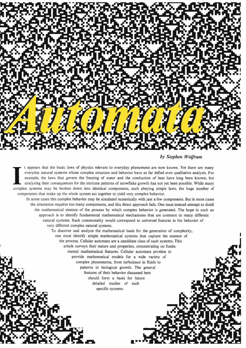
t appears that the basic laws of physics relevant to everyday phenomena are now known. Yet there are many

everyday natural systems whose complex structure and behavior have so far defied even qualitative analysis. For

example the laws that govern the freezing of water and the condu ction of heat have long been known but

analyz ing their conseq uences for the intricate patterns of snow flake growth has n ot yet been possible. While man y

complex systems may be broken down into identical com ponents each obeying simple laws the huge numb er of

components that make up the whole system act together to yield very complex behavior.

In som e cases this com plex behavior may be simulated numerically with just a few components. But

n

most cases

the simulation requires too many co mpon ents and this direct approach fails. One must instead attem pt to distill

the mathematical essence of the process by which complex behavior is generated. The hope in such an

approach is to identify fundamental mathematical mechanisms that are common to many different

natural systems. Such commonality would correspond to universal features in the behavior of

very different complex natural systems.

To discover and analyze the mathematical basis for the generation of complexity

one must identify simple mathematical systems that capture the essence of

the process. Cellular automata are a candidate class of such systems. This

article surveys their nature and properties conce ntrating on funda-

mental mathematical features. Cellular automata promise to

provide mathematical models for a wide variety of

complex phenomema from turbulence in fluids to

patterns in biological growth. The general

features of their behavio r discussed here

should form a basis for future

detailed stu die s of such

specific systems.



The

ature

of Cellular utomata

and

a

Simple Example

Cellular automata are simple mathemati-

cal idealizations of natural systems. They

consist of a lattice of discrete identical sites,

each site taking on a finite set of, say, integer

values. The values of the sites evolve in

discrete time steps according to deterministic

rules that specify the value of each site in

terms of the values of neighboring sites.

Cellular automata may thus be considered as

discrete idealizations of the partial differen-

tial equations often used to describe natural

systems. Their discrete nature also allows an

important analogy with digital computers:

cellular automata may be viewed as parallel-

processing computers of simple construction.

As a first example of a cellular automaton,

consider a line of sites, each

with

value

0

or

1

(Fig. 1 . Take the value of a site at position i

on time step

t

to be

a:

One very simple rule

for the time evolution of these site values is

mod

2

where mod 2 indicates that the 0 or 1

remainder after division by

2

is taken. Ac-

cording to this rule, the value of a particular

site is given by the sum modulo

2

(or,

equivalently, the Boolean algebra exclusive

or ) of the values of its left- and right-hand

nearest neighbor sites on the previous time

step. The rule is implemented simultaneously

at each site.* Even with this very simple rule

quite complicated behavior is nevertheless

found.

Fractal Patterns Grown from Cellular Au-

tomata. First of

all

consider evolution ac-

In

the

very

simplest computer implement tion a

separate

rr y

o f qdated site

values

must e

maintained and copied

back

to the original site

value

rr y when

the upd ting process s com-

plete.

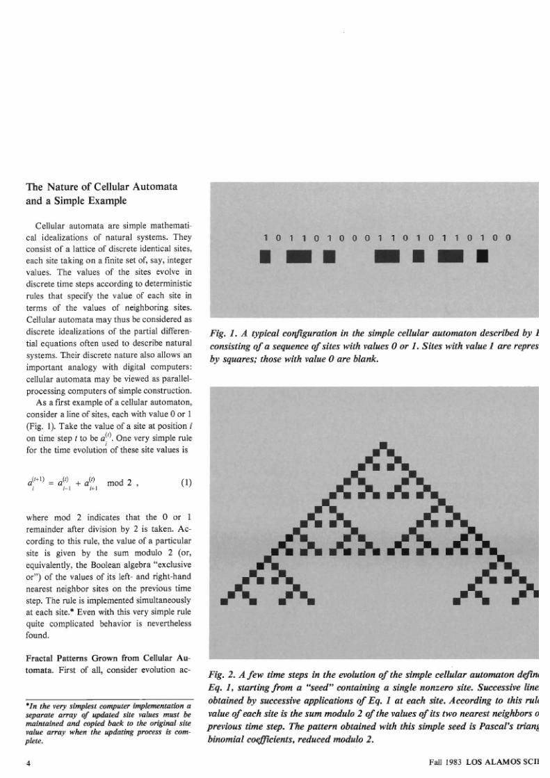
Fig. 1.

A

typical configuration in the simple cellular automaton described by

E

consisting of a sequence of sites with values 0 or

1 .

Siteswith value 1

are

repres

by squares; those with value 0 are blank.

Fig. 2

A

few time steps in the evolution of the simple cellular automaton defin

Eq 1 starting rom a seed containing a single nonzero site. Successive line

obtained by successive applications of

Eq

1 at each site. According to this

rule

value qf each site s the sum modulo 2

qf

he values of its two nearest neighbors o

previous time step. Thepattern obtained with th is simple seed

is

Pascal's triang

binomial coefficients, reduced modulo 2

Fall 983

LOS

L MOS S IE



CellularAutomata

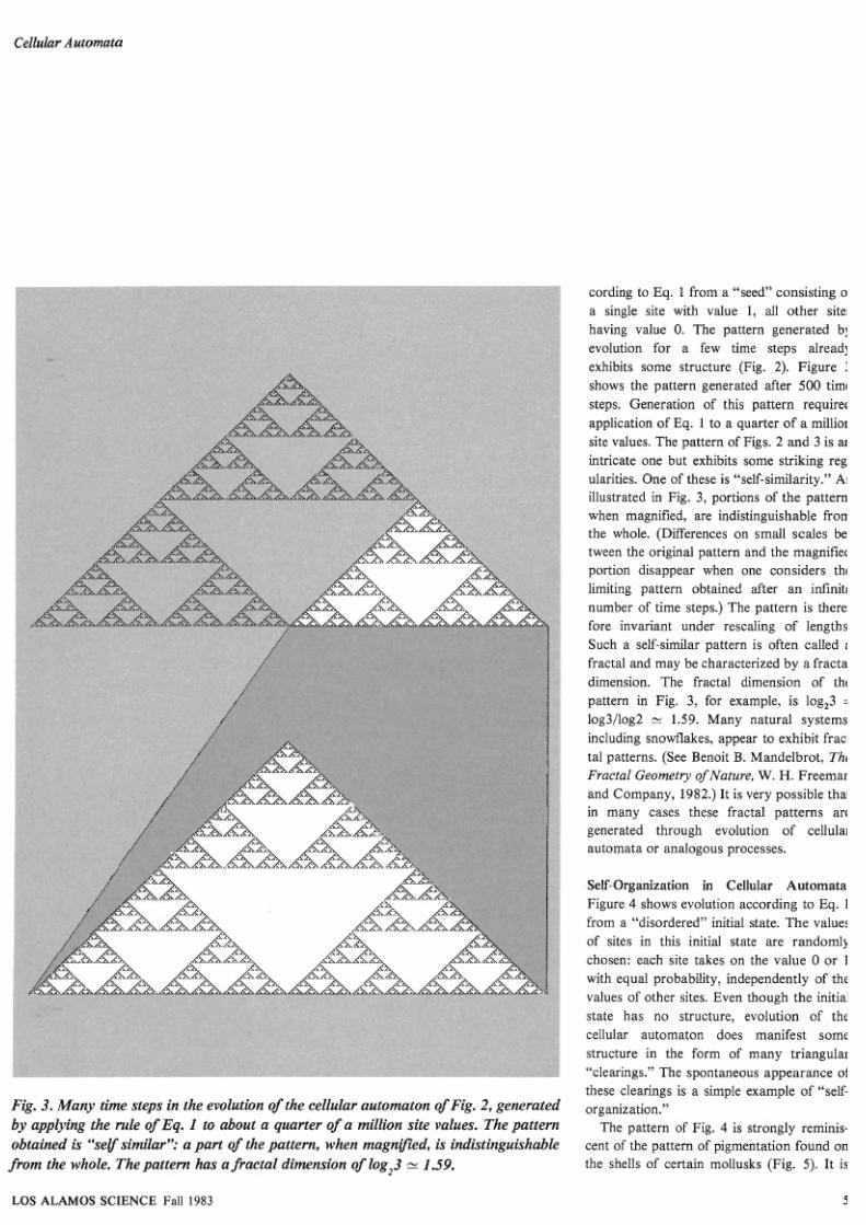
Fig.

3.

Many tune steps in the evolution

of

the cellular automaton o f Fig. 2 generated

by applying the rule of Eq.

1

to about quarter of a million site values. The pattern

obtained is self similar*': a part of

the

pattern, when magnified, is indistinguishable

from the whole. The pattern has a fractal dimension of l o g 3 1.59.

cording to Eq. 1 from a seed consisting of

a single site with value 1, all other sites

having value

0.

The pattern generated by

evolution for a few time steps already

exhibits some structure (Fig. 2). Figure 3

shows the pattern generated after

500

time

steps. Generation of this pattern required

application of Eq. 1 to a quarter of a million

site values. The pattern of Figs. 2 and 3 is an

intricate one but exhibits some striking reg-

ularities. One of these is self-similarity. As

illustrated in Fig.

3,

portions of the pattern

when magnified, are indistinguishable from

the whole. (Differences on small scales be-

tween the original pattern and the magnified

portion disappear when one considers the

limiting pattern obtained after an intmite

number of time steps.) The pattern is there

fore invariant under rescaling of lengths

Such a self-similar pattern is often called a

fractal and may be characterized by a fracta

dimension. The fractal dimension of the

pattern in Fig.

3

for example, is log23

log3/log2 1 59 Many natural systems

including snowflakes, appear to exhibit frac-

tal patterns. (See Benoit B. Mandelbrot,

The

Fractal Geometry ofNature W .H Freeman

and Company, 1982.) It is very possible that

in many cases these fractal patterns are

generated through evolution of cellular

automata or analogous processes.

Self-organization

in

Cellular Automata

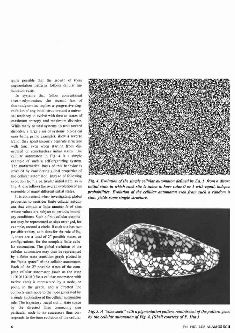
Figure 4 shows evolution according to Eq.

1

from a disordered initial state. The values

of sites in this initial state are randomly

chosen: each site takes on the value 0 or 1

with equal probability, independently of the

values of other sites. Even though the initial

state has no structure, evolution of the

cellular automaton does manifest some

structure in the form of many triangular

'clearings. The spontaneous appearance of

these clearings is a simple example of self-

organization.

The pattern of Fig. 4 is strongly reminis-

cent of the pattern of pigmentation found on

the shells of certain mollusks (Fig. 5). It is

LOS ALAMOS SCIENCE

Fall

983



quite possible that the growth of these

pigmentation patterns follows cellular au-

tomaton rules.

In systems that follow conventional

thermodynamics, the second law of

thermodynamics implies a progressive deg-

radation of any initial structure and a univer-

sal tendency to evolve with time to states of

maximum entropy and maximum disorder.

While many natural systems do tend toward

disorder, a large class of systems, biological

ones being prime examples, show a reverse

trend: they spontaneously generate structure

with time, even when starting from dis-

ordered or structureless initial states. The

cellular automaton in Fig.

4

is a simple

example of such a self-organizing system.

The mathematical basis of this behavior is

revealed by considering global properties of

the cellular automaton. Instead of following

evolution from a particular initial state, as in

Fig.

4,

one follows the overall evolution of an

ensemble of many different initial states.

It is convenient when investigating global

properties to consider finite cellular autom-

ata that contain a finite number N of sites

whose values are subject to periodic bound-

ary conditions. Such a finite cellular automa-

ton may be represented as sites arranged, for

example, around a circle. If each site has two

possible values, as it does for the rule of Eq.

1 there are a total of N possible states, or

configurations, for the complete finie cellu-

lar automaton. The global evolution of the

cellular automaton may then be represented

by a finite state transition graph plotted in

the state space of the cellular automaton.

Each of the N possible states of the com-

plete cellular automaton (such as the state

11 1 11 1 1 for a cellular automaton wit

twelve sites) is represented by a node, or

point, in the graph, and a directed line

connects each node to the node generated by

a single application of the cellular automaton

rule. The trajectory traced out in state space

by the directed lines connecting one

particular node to its successors thus cor-

responds to the time evolution of the cellular

Fig.

4.

Evolution of the simple cellufar automaton defined byEq 1,from a disord

initial state in which each site is taken to have value

0

or

1 with equal, indepen

probabilities. Evolution of the cellular automaton even from such a random in

state yields some

simp e structure

Fig.

5 A

cone shell with apigmentationpattern reminiscent of the pattern gener

by the cellular automaton of Fig. 4 (Shell courtesy of

P

Hut.)

Fall

983

LOS L MOS SCI



Cellular

Automata

automaton from the initial state represented

by that particular node. The state transition

graph of Fig. 6 shows all possible trajectories

in statei,space for a cellular automaton with

twelve sites evolving according to the simple

rule of

Eq. 1.

A

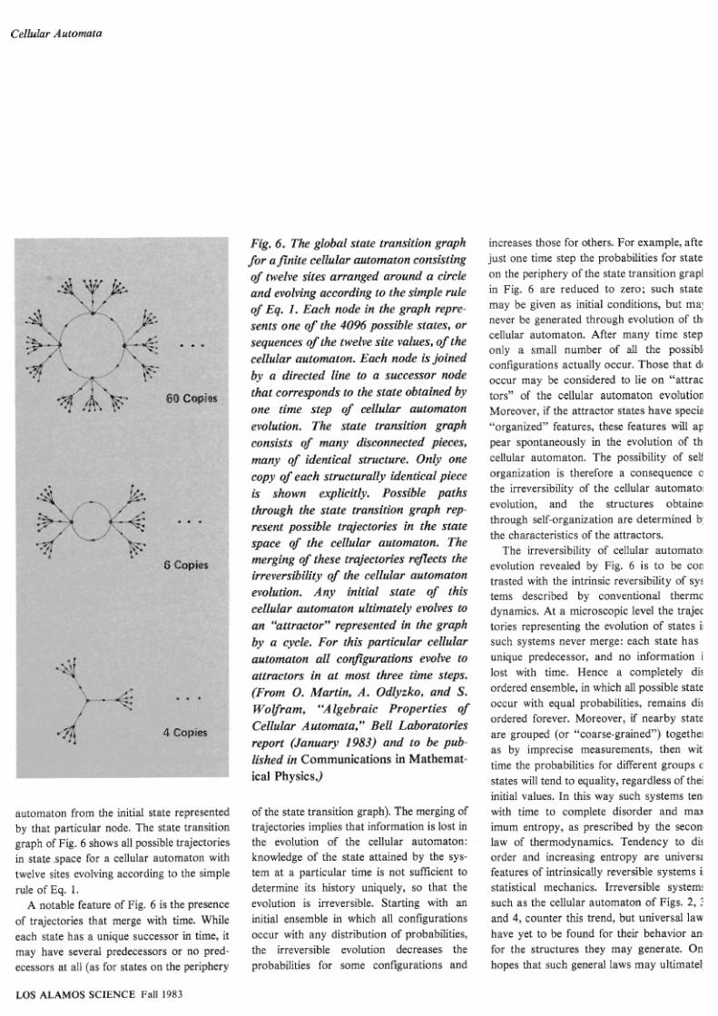
notable feature of Fig. 6 is the presence

of trajectories that merge with time. While

each state has a unique successor in time, it

may have several predecessors or no pred-

ecessors at all

(as

for states on the periphery

Fig. 6.

he

global state transition graph

for a inite cellular automaton consisting

of twelve sites arranged around a circle

and evolving according to the simple rule

of

Eq

1. Each node in the graph repre-

sents one of the 4096 possible states, or

sequences of the twelve site values, of the

cellular automaton. Each node s oined

by a directed line to a successor node

that corresponds to

th

state obtained by

one time step o f cellular automaton

evolution. The state transition graph

consists of many disconnected pieces,

many of identical structure. Only one

copy of each structurally identical piece

is shown explicitly. Possible paths

through the state transition graph rep-

resent possible trajectories in the state

space of the cellular automaton. The

merging of these trajectories reflects the

irreversibility of the cellular automaton

evolution. Any initial state o this

cellular automaton ultimately evolves to

an attractor represented in the graph

by a cycle. For this particular cellular

automaton all configurations evolve to

attractors in at most three time steps.

(From 0 Martin, A. Odlyzko, and

S.

Wolfram, Algebraic Properties of

Cellular Automata, Bell Laboratories

report (January 1983 and to be pub-

lished in Communications in Mathemat-

ical Physics.

of the state transition graph). The merging of

trajectories implies that information is lost

in

the evolution of the cellular automaton:

knowledge of the state attained by the sys-

tem at a particular time is not sufficient to

determine its history uniquely, so that the

evolution is irreversible. Starting with an

initial ensemble in which all configurations

occur with any distribution of probabilities,

the irreversible evolution decreases the

probabilities for some configurations and

increases those for others. For example, afte

just one time step the probabilities for state

on the periphery of the state transition grap

in Fig. 6 are reduced to zero; such state

may be given as initial conditions, but ma

never be generated through evolution of th

cellular automaton. After many time step

only a small number of all the possibl

configurations actually occur. Those that d

occur may be considered

to

lie on attrac

tors of the cellular automaton evolution

Moreover, if the attractor states have speci

organized features, these features

will

ap

pear spontaneously in the evolution of th

cellular automaton. The possibility of self

organization is therefore a consequence o

the irreversibility of the cellular automato

evolution, and the structures obtaine

through self-organization are determined b

the characteristics of the attractors.

The irreversibility of cellular automato

evolution revealed by Fig. 6 is to be con

trasted with the intrinsic reversibility of sys

tems described by conventional thermo

dynamics. At a microscopic level the trajec

tories representing the evolution of states i

such systems never merge: each state has

unique predecessor, and no information i

lost with time. Hence a completely dis

ordered ensemble, in which

all

possible state

occur with equal probabilities, remains dis

ordered forever. Moreover, if nearby state

are grouped (or coarse-grained ) togethe

as by imprecise measurements, then wit

time the probabilities for different groups o

states will tend to equality, regardless of the

initial values. In this way such systems ten

with time to complete disorder and max

imum entropy, as prescribed by the secon

law of thermodynamics. Tendency to dis

order and increasing entropy are universa

features of intrinsically reversible systems i

statistical mechanics. Irreversible system

such as the cellular automaton of Figs. 2 3

and 4 counter this trend, but universal law

have yet to be found for their behavior an

for the structures they may generate. ne

hopes that such general laws may ultimatel

LOS ALAMOS SCIENCE Fall

1983



For odd N, II may be shown to divide

e abstracted from an investigation of the

ing for each configuration a characteristic

Q2 2k+l) 211N=2k+

comparatively simple examples provided by polynomial

cellular automata.

While there is every evidence that the

N

fundam ental microscopic laws of physics are = a i x i

,

intrinsically reversible (information-preserv-

i=o

ing, though not precisely time-reversal in-

variant), many systems behave

where x is a dummy variable, and the

and n fact is almost always equal to

On a

macroscopic scale

and

are ap- coefficient of xi is the value of the site at

value (the first exception occurs for N

propriatell'

described

by h eve rsible laws.

position i. I n terms of charac teristic poly- Here sordJ2) is a num ber theoretical

the

molecu-

nomials, the cellular automaton rule of Eq. 1

tion defined to be the minimum po

lar interactions in a fluid are entirely re-

takes

on

the particularly simple

form

integ er for which 2-7

=

Â1 modulo

N

versible, macroscopic descriptions of the

maximum value of sordy(2), typ

average velocity field in the fluid, using, say,

achieved when N is prime, is (N-l)/2.

the Navier-Stokes equations, are irreversible = T(~)A '*) (~)

(#-

l )

,

maximal cycle length is thus of order 2

and contain dissipative terms. Cellular au-

approximately the square root of the

tomata provide mathematical models at this

where

number of possible states 2^.

mac roscopic level.

An unusual feature of this analysis

T(x) = (x x-l)

appearance of number theoretical con

Number theory is inundated with com

Mathematical Analysis of a Simple

results based on very simple premis

Cellular Automaton

and all arithmetic on the polynomial coeffi-

may be part of the mathematical mecha

cients is performed modulo

2

The reduction by which natu ral system s of simple cons

modulo -I implements periodic boundary

tion yield complex behavior.

The cellular automaton rule of Eq. 1 is

conditions. The structure of the state tran-

particularly simple and admits a rather corn-

sition diagram may then be deduced from

plete m athem atical analysis.

algebraic properties of the polynomial n x ).

hh re (h ler al Cellular Automat

The fractal patterns of Figs. 2 and 3 may

For even

N

one finds, for example, that the

be characterized in a simple algebraic man-

fraction of states on attractors is 2-^W,

ner. If no reduction modulo 2 were Per-

where D.,(N) is defmed as the largest integral

formed, then the values of sites generated

power of 2 tha t divides (for example,

The discussion so far has concentrat

from a single nonzero initial site would

D ( 1 2 ) = 4 .

the particular cellular automaton rule

simply be the integers appearing in I%scal's

Since a finite cellular automaton evolves

by Eq. 1. This rule may be generaliz

triangle of binomial coefficients. The pattern

deterministically with a finite total number of

several ways. On e family of rules is obt

of nonzero sites in Figs. 2 and 3 is therefore

possible states, it must ultimately enter a

by allowing the value of a site to b

t h e pattern of odd binomial coefficients in cycle in which it visits a sequence of states arbitrary function of the values of the

hs ca l' s triangle- (See Stephen Wolfram,

repeatedly. Such cycles are manifest as

itself and of its two nearest neighbors o

"Geometry of Binomial Coefficients," to be

closed loops in the state transition graph.

previous time step:

published in Ame rican Mathe matical

Monthly.)

This algebraic approach may be extended

to determine the structure of the state tran-

sition diagram of Fig.

6.

(See 0 Ma rtin, A.

Odlyzko, and S. Wolfram, "Algebraic

Properties of Cellular Automata," Bell Labo -

ratories report (January 1983) and to be

published in Comm unications in Math ema ti-

cal Physics.) The analysis proceeds by writ-

The algebraic analysis of M artin et al. shows

that for the cellular automaton of Eq.1 the a(. ) ~(a a( ')

(

,

j

maximal cycle length

11

(of which

all

other

cycle lengths are d ivisors) is given for even N

by

A convenient notation illustrated in F

assigns a "rule number" to each of the

rules of this type. The rule num ber of

Eq

90

in

this notation.

Further generalizations allow each s

a cellular automaton to take on an arb

Fall 1983

LOS L MOS SCIE



Cellular

Automata

Universality

lasses in Cellular

utomata

flute

~

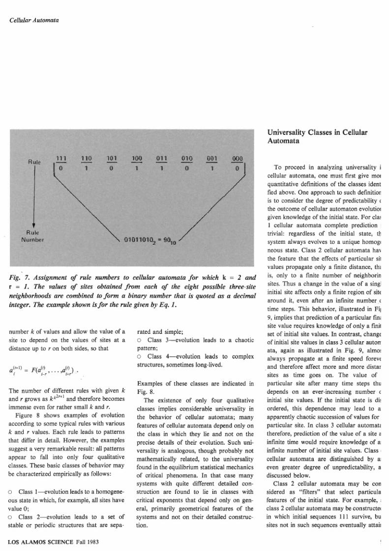
Fig 7 Assignment of

rule

numbers to cellular automata for which k and

r I . The values o f sites obt ined from each

o f

the eight possible

three site

neigh orhoods

are combined to form a binary number that s

quoted

as a decimal

integer

The example

shown

is

for

the

rule given

by Eq 1

number k of values and allow the value of a

site to depend on the values of sites at a

distance up to

r

on both sides, so that

The number of different rules with given

k

and r

grows as

kk2r 1

nd therefore becomes

immense even for rather small k and r.

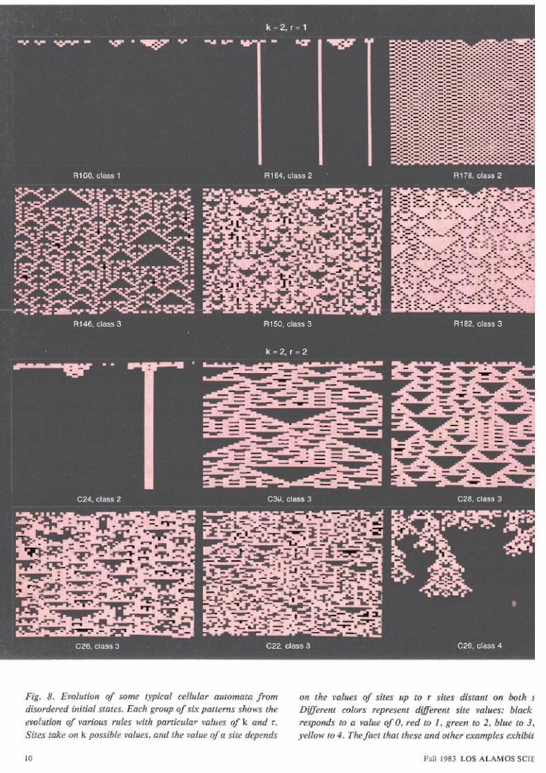
Figure 8 shows examples of evolution

according to some typical rules with various

k

and r values. Each rule leads to patterns

that differ in detail. However, the examples

suggest a very remarkable result: all patterns

appear to fall into only four qualitative

classes. These basic classes of behavior may

be characterized empirically as follows:

o Class 1-evolution leads to a homogene-

ous state in which, for example,

all

sites have

value 0;

Class 2-evolution leads to a set of

stable or periodic structures that are sepa-

rated and simple;

o

Class 3-evolution leads to a chaotic

pattern;

o Class 4-evolution leads to complex

structures, sometimes long-lived.

Examples of these classes are indicated in

Fig. 8.

The existence of only four qualitative

classes implies considerable universality in

the behavior of cellular automata; many

features of cellular automata depend only on

the class in which they lie and not on the

precise details of their evolution. Such uni-

versality is analogous, though probably not

mathematically related, to the universality

found in the equilibrium statistical mechanics

of critical phenomena. In that case many

systems with quite different detailed con-

struction are found to lie in classes with

critical exponents that depend only on gen-

eral, primarily geometrical features of the

systems and not on their detailed construc-

tion.

To proceed in analyzing universality i

cellular automata, one must first give mor

quantitative definitions of the classes ident

fied above. One approach to such definition

is to consider the degree of predictability o

the outcome of cellular automaton evolutio

given knowledge of the initial state. For clas

1 cellular automata complete prediction

trivial: regardless of the initial state, th

system always evolves to a unique homoge

neous state. Class

2

cellular automata hav

the feature that the effects of particular sit

values propagate only a finite distance, tha

is, only to a finite number of neighborin

sites. Thus a change

in

the value of a singl

initial site affects only a finite region of site

around it, even after an infinite number o

time steps. This behavior, illustrated in Fig

9

implies that prediction of a particular fina

site value requires knowledge of only a finit

set of initial site values.

In

contrast, change

of initial site values

in

class

3

cellular autom

ata, again as illustrated

in

Fig. 9, almo

always propagate at a finite speed foreve

and therefore affect more and more distan

sites as time goes on. The value of

particular site after many time steps thu

depends on an ever-increasing number o

initial site values. If the initial state is dis

ordered, this dependence may lead to a

apparently chaotic succession of values for

particular site.

In

class

3

cellular automata

therefore, prediction of the value of a site a

infmite time would require knowledge of

a

infinite number of initial site values. Class

cellular automata are distinguished by a

even greater degree of unpredictability, a

discussed below.

Class 2 cellular automata may be con

sidered as filters that select particula

features of the initial state. For example, a

class 2 cellular automata may be constructed

in which initial sequences 111 survive, bu

sites not

in

such sequences eventually attain

LOS L MOS SCIENCE Fall

983



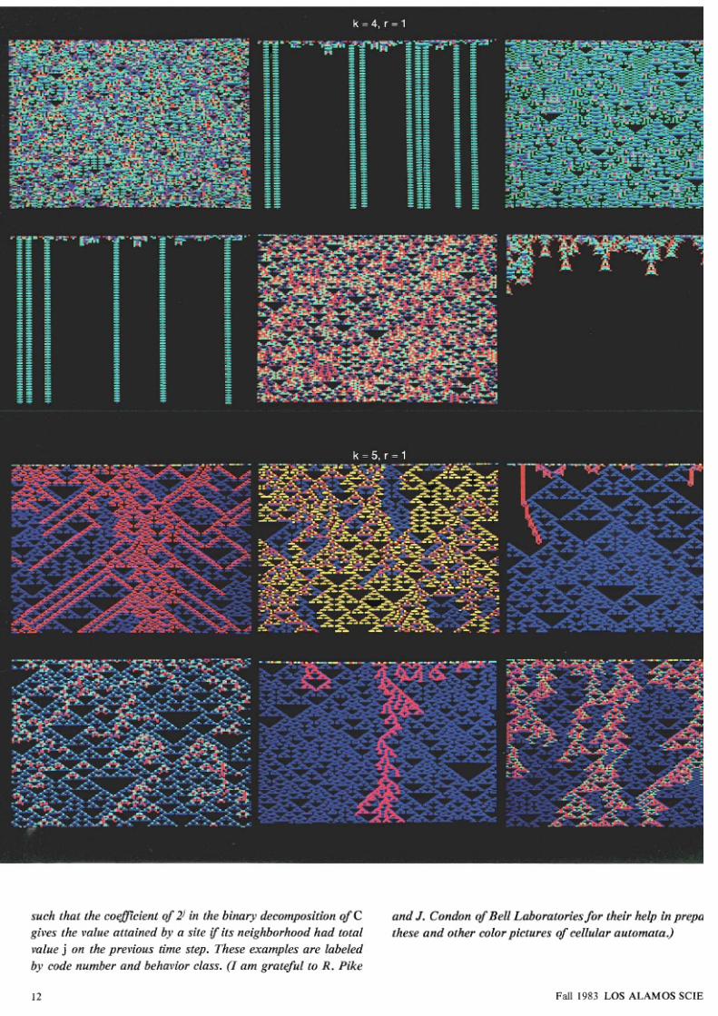
Fig. 8 Evolution of some typical cellular automata fro m

on the values of sites up to r sites distant

on

both s

disordered initial states. Each group of s x patterns shows the

Different colors represent different site values: black

evolution of various rules w ith particular values of k and

r

responds to a value of 0 red

to 1

green

to

2 blue

to

3

Sites take on k possible values and the value of a site depends

yellow to

4 .

The/act that these and other

examples

exhibit

1 all 983 LOS ALAMOS SCIE



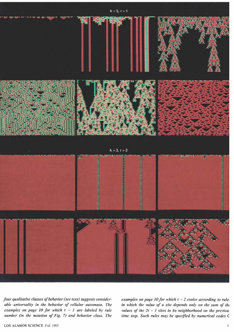
four qualitative classes of behavior see text) suggests consider-

examples on page

10

for which r

2

evolve according to rule

able universality in the behavior of cellular automata. The

in which the value of site depends

only

on the sum of

th

examples on page 10 for which r 1 are labeled by rule

values o

the

2r

1 sites in its neighborhood on the previou

number in the notation of Fig. 7 and behavior class. The

tim

step. Such rules may be specvied by numerical

odes

LOS ALAMOS SCIENCE Fall 983



such that the co ^cient

of f

in the binary decom position qf

and J . Condon o f Bell Laboratoriesfor their help in prep

gives the value attained

by

a site i tsneighborhood had total

these and other color pictures o f cellular autom ata.)

value on the previous time step. These examples are labeled

by code number and behavior class.

Iam

grateful

to R

Pike

2

Fall 983 LOS L MOS S IE



I

lass 2

class

4 class 4

Fig.

9

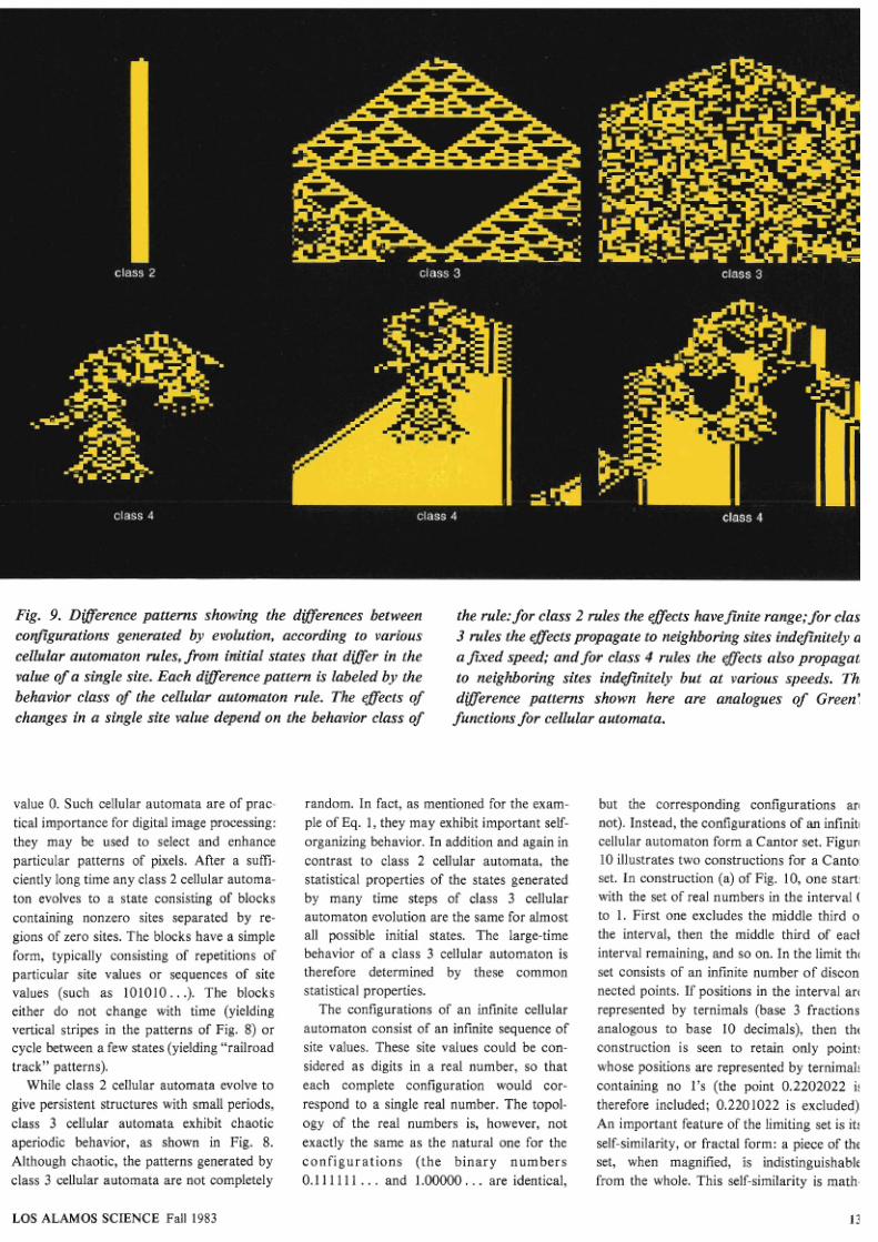
Difference patterns showing the differe nces between

the rule: for class

2

rules the effects have finite range;for clas

configurations generated by evo lution, according to various

3 rules the effects propag ate to neighboring sites indefinitely a

cellular automaton rules, from initial states that d iff er n the

a fixed speed; and for class

4

rules the effects also propagate

value of a single sit e. Each deference pattern is labeled by the

to neighboring sites indefinitely but at various speeds. Th

behavior class of the cellular au tomato n rule. The effe cts of

difference patterns shown here are analogues of Green

changes in a single site value depend on the behavior class of functions for cellular autom ata.

value 0. Such cellular autom ata ar e of prac-

tical impo rtance for digital image processing:

they may

be

used to select and enhance

particular patterns of pixels. After a suffi-

ciently long time any c lass 2 cellular automa-

ton evolves to a state consisting of blocks

containing nonzero sites separated by re-

gions of zero sites. The blocks ha ve a simple

form, typically consisting of repetitions of

particular site values or sequences of site

values (such as 10 10 10 . . The blocks

either do not change with time (yielding

vertical stripes in the patterns of Fig. 8) or

cycle between a few states (yielding railro ad

track patterns).

While class 2 cellular automata evolve to

give persistent structures with small periods,

class

3

cellular automata exhibit chaotic

aperiodic behavior, as shown in Fig. 8.

Although chaotic, the patterns generated by

class 3 cellular automata are not completely

random.

In

fact, as mentioned for the exam-

ple of Eq. 1 they m ay exhibit impo rtant self-

organizing behavior. In addition and again in

contrast to class 2 cellular automata, the

statistical properties of the states generated

by many time steps of class

3

cellular

automaton evolution are the same for almost

all possible initial states. The large-time

behavior of a class 3 cellular automaton is

therefore determined by these common

statistical properties.

The configurations of an infinite cellular

automaton consist of an infinite sequence of

site values. These site values could be con-

sidered as digits in a real number, so that

each complete configuration would cor-

respond to a single real number. The topol-

ogy of the real numbers is, however, not

exactly the same as the natural one for the

co n f i g u r a t i o n s ( t h e b i n a r y n u m b er s

0.111 1 1 and 1.00000 are identical,

but the corresponding configurations ar

not). Instead, the c onfigurations of an infinit

cellular automaton form a Cantor set. Figur

10 illustrates two constructions for a C anto

set. In co nstruction (a) of Fig. 10 one start

with the set of real numbers

in

the interval

to 1 First o ne excludes the middle third o

the interval, then the middle third of each

interval remaining, and so on. In th e limit th

set consists of an infinite number of discon

nected points. If positions in the interval ar

represented by ternimals (base

3 fractions

analogous to base 10 decimals), then th

construction is seen to retain only point

whose positions are represented by ternimal

containing no 1's (the point 0.2202022 i

therefore included; 0.2201022 is excluded)

n

importan t feature of th e limiting set is it

self-similarity, or fractal form: a piece of the

set, when magnified, is indistinguishabl

from the whole. This self-similarity is math-

LOS

ALAMOS

SCIENCE Fall 983



ematically analogous to that found for the

limiting two-dimensional pattern of Fig. 3.

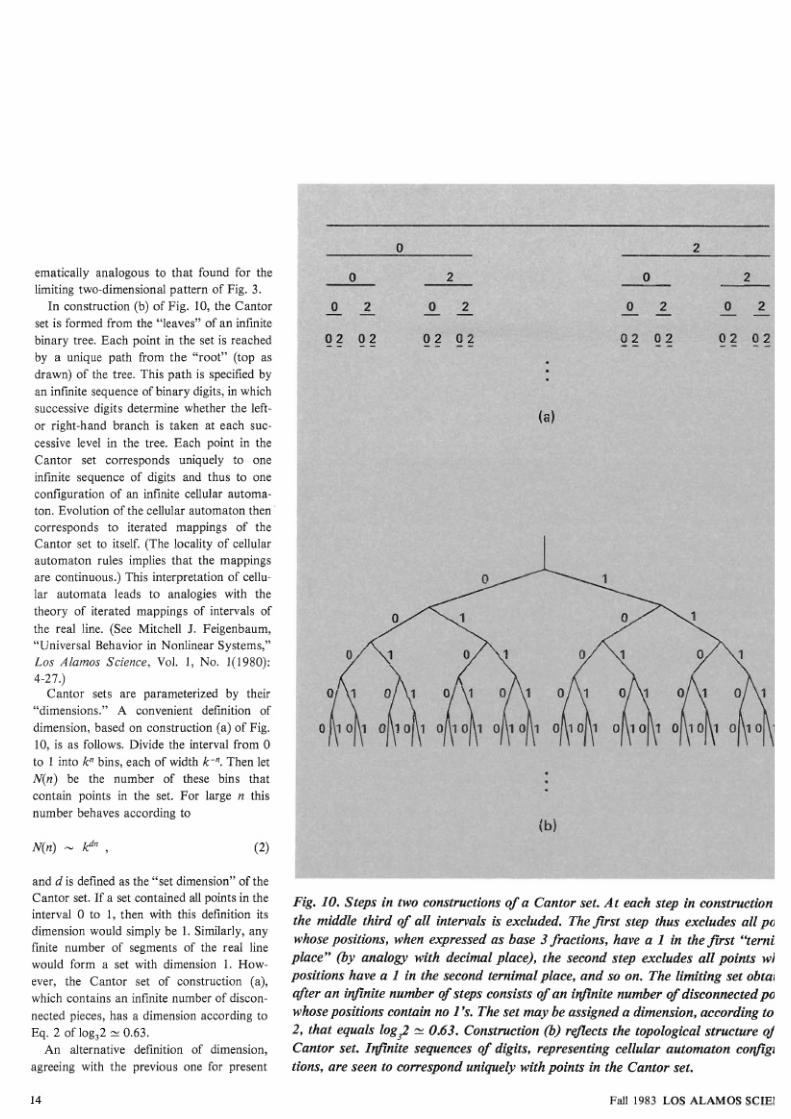
In construction (b) of Fig. 10, the Cantor

set is formed from the leaves of an infinite

binary tree. Each point in the set is reached

by a unique path from th e root (top as

drawn) of the tree. This path is specified by

an infinite sequence of binary digits, in which

successive digits determine whether the left-

or right-hand branch is taken at each suc-

cessive level n the tree. Each point in the

Cantor set corresponds uniquely to one

idmite sequence of digits and thus to one

configuration of an infinite cellular automa-

ton. Evolution of the cellular automaton then.'

corresponds

to iterated mappings of the

Cantor set to itself. (The locality of cellular

automaton rules implies that the mappings

are continuou s.) This interpretation of cellua

lar automata leads to analogies with the

theory of iterated mappings of intervals of

the real line. (See Mitchell

J.

Feigenbaum,

Universal Behavior in N onlinear Systems,

os Alamos Scien ce, Vol. 1, No. l (1980):

4-27.)

Cantor sets are parameterized by their

dimensions. A convenient definition of

dimension, based on construction (a) of Fig.

10, is as follows. Divide the interval from 0

to 1 nto

kn

bins, each of width k- .Then let

N n)

be the number of these bins that

contain points in the set. For large n this.

number behaves according to

and d is defined as the set dimension of th e

Can tor set. If a set contained ll points in the

interval 0 to 1, then with this definition its

dimension would simply be 1. Similarly, any

finite number of segments of the real line

would form a set with dimension

1. How-

ever, the Cantor set of construction (a),

which contains a n infinite number of

discon-

E h b c t e d pieces , has a d imension according to

Eq. 2 of log32

=

0.63.

An alternative definition of dimension,

&a gr ee in g with the previous one for present

Fig. 10, Steps in two constructions of a Cantor set. At each step in construction

the middle third of all intervals is excluded.

The

first step thus excludes all po

whose positions, when expressed as base 3 fractions, have a 1 in the first temi

place by analogy with decimal place), the second step excludes all points wh

posit10ns have a 1 in the second temimalplace, and so on. The limiting set obta

qfter an infinite number of steps consists of a n infinite number of disconnected po

whose positions contain no 1 's.

The

set

m y

be assigned a dimension, according to

2

that equals log3 = 0.63. Construetion b) reflects the topological structure of

Cantor set. Ivtfinite sequences of digits, representing cellular automaton config

tions, are seen to correspond uniquely with

DO&

in the Cantor set.

Fall

983 LOS

L MOS S IE



ellular

Automata

equation

z2

Is. 1

= 0. (See

D A

Und

Applications of Ergodic Theory

an

Sofie Systems to Cellular Automata,

Un

wsity of

Washington

preprint (April 198

and to be published in hysics

D;

see

al

Martin et al

op. cit. The greater th

1

irreversibility in the cellular automaton ev

1

lution, the smaller is the dimension of th

Cantor set corresponding

to

the attracto

for the evolution. If theset of attractors for

cellular automaton

has

dimension 1,

the

essentially

ll the

configurations of th

cellular automaton may occur at large

time

purposes, is based on self-similarity. Take

the Cantor set of construction (a) in Fig. 10.

Contract the set by a magnification factor

k-1 . By virtue of its self-similarity, the whole

set is identical to a number, say M(m), of

copies of this contracted copy. For large m,

M(m) w f^ *, where again

d

is defined as the

set dimension.

With these definitions the dimension of the

Cantor set of all possible configurations for

an S i t e one-dimensional cellular automa-

ton is 1. A disordered ensemble, in which

each possible configuration occurs with

equal probability, thus has dimension

1.

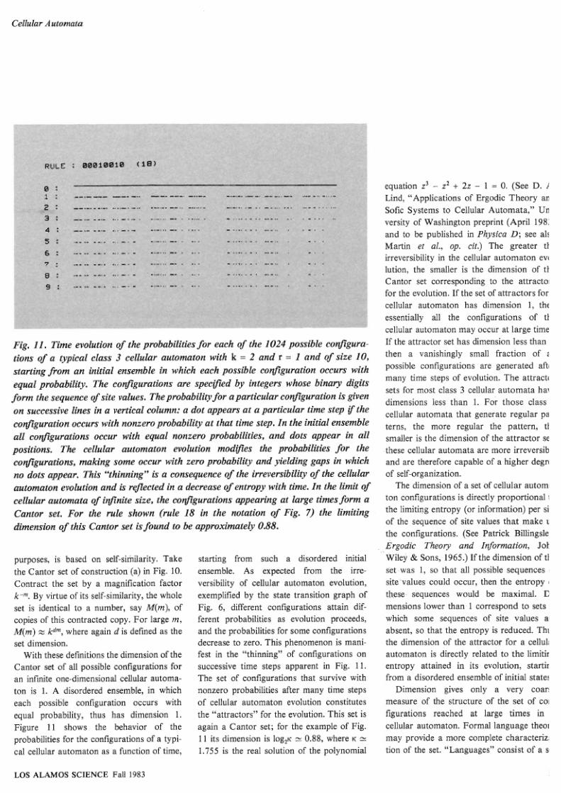
Figure 11 shows the behavior of the

probabilities for the configurations of a typi-

cal cellular automaton as a function of time,

starting from such a disordered initial

ensemble. As expected from the irre-

versibility of cellular automaton evolution,

exemplified by the state transition graph of

Fig.

6

different configurations attain dif

ferent probabilities as evolution proceeds,

and the probabilities for some configurations

decrease to zero. This phenomenon is mani-

fest in the thinning of configurations on

successive time steps apparent in Fig.

11.

The set of configurations that survive with

nonzero probabilities after many time steps

of cellular automaton evolution constitutes

the ccattractors or the evolution. This set is

again a Cantor set; for the example of Fig.

11 its dimension is log ^ =0.88, where K

=

1.755

is the real solution of the polynomial

odic

Theory and Information, Joh

W i h y Sons 1965.)

If

the dimemion of t

setwas 1 so

that

all possible sequences

gitebalues could occur

them

the entropy

sequences would be maximal.

D

mensions lower than 1 correspond

to

sets

wfaiefa some sequences of site values

a

absent

so

that the

entropy

is

reduced.Th

the

dimension of

the

attractor

for

a cellul

automaton is directly

related to the limiti

entropy attained in its evolution, startin

from a disordered ensemble

of

initi l states

Dimension gives only a

very

coar

measure of the structure of the set of eo

figurations reached at large times in

cellular automaton. Formal

anguage

theo

may provide a more complete characteriz

tion of the set. Languages consist

of

a s




of words, typically infinite in number,

formed from a sequence of letters according

to certain grammatical rules. Cellular

automaton configurations are analogous to

words in a formal language whose letters are

the k possible values of each cellular automa-

ton site.

A

grammar then gives a succinct

specification for a set of cellular automaton

configurations.

Languag es may be classified according to

the complexity of the machines or compu ters

necessary to generate them. A simple class

of languages specified by regular gram-

mars may

be

generated by finite state

machines. A finite state machine is repre-

sented by a state transition graph (analogous

to the state transition graph for a finite

cellular autom aton illustrated

in

Fig.

6 .

The

possible words in a regular grammar are

generated by traversing all possible paths

in

the state transition graph. These words may

be specified by regular expressions consist-

ing of finite length sequences and arbitrary

repetitions of these. For example, the regular

expression 1(00)* represents all sequences

containing an even number of 0's (arbitrary

repetition of the sequence 00) flanked by a

pair of 1's. The set of conf igura tions ob-

tained at large times in class 2 cellular

automata is found to form a regular lan-

guage. It is likely that attractors for other

classes of cellular automata correspond to

more complicated languages.

Analogy with Dynamical

Systems Theory

The three classes of cellular automaton

behavior discussed so far are analogous to

three classes of behavior found

in

the solu-

tions to differential equations (continuous

dynamical systems). For some differential

equations the solutions obtained with any

initial conditions approach a fixed point at

large times. This behavior is analogous to

class 1 cellular automaton behavior. In a

second class of differential equations, the

limiting solution at large times is a cycle in

which the parameters

vary

periodically with

time. These equations are analogo us to class

2 cellular automata. Finally, some differen-

tial equations have been found to exhibit

complicated, apparently chao tic behavior de-

pending in detail on their initial conditions.

With the initial conditions specified by deci-

mals, the solutions to these differential equa-

tions depend on progressively higher

and

higher order digits in the initial conditions.

This phenomenon is analogous to the de-

pendence of a particular site value on pro-

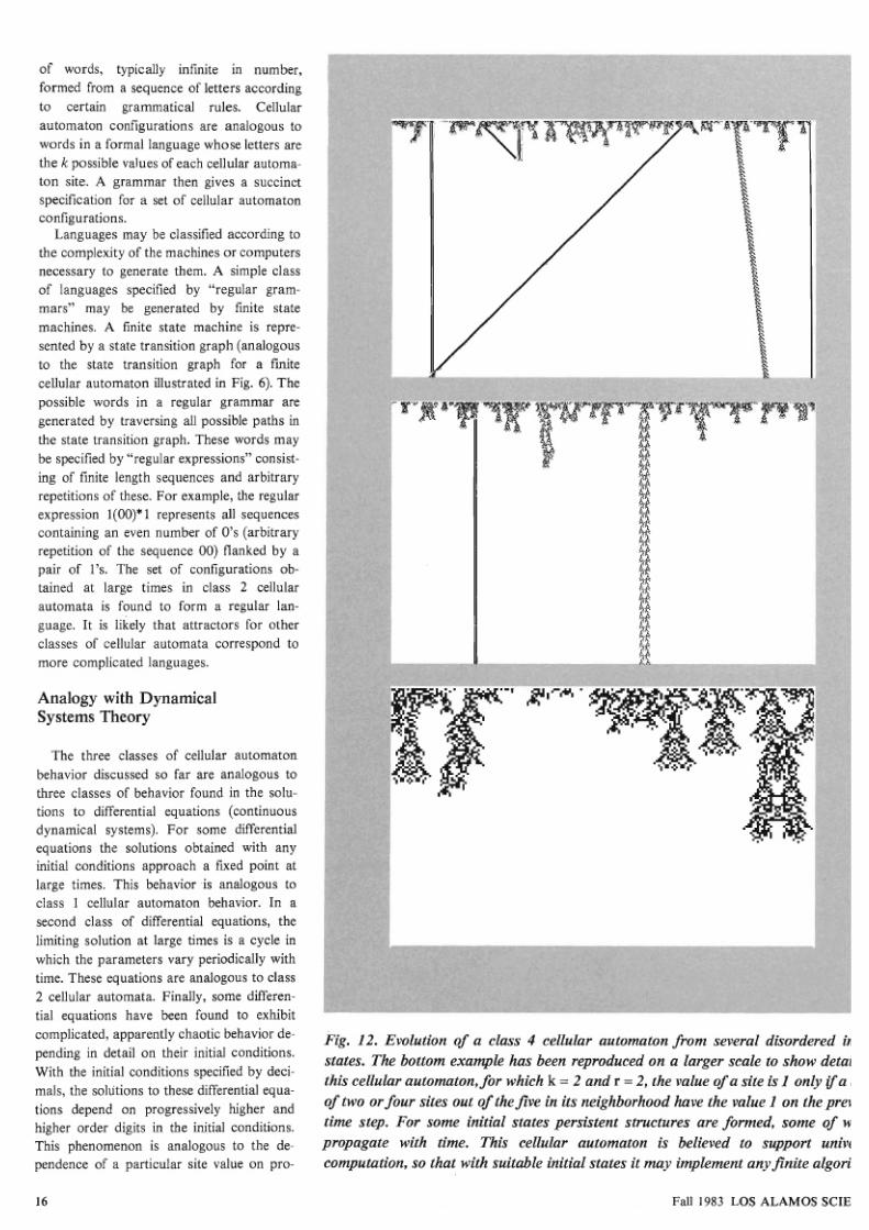
Fig. 12 . Evolution of a class 4 cellular automaton from several disordered in

states. The bottom example has been reproduced on a larger scale to show d etai

this cellular automaton or which

k

2 and

r

2 the value of a site is only f a

of two or four sites out of the five in its neighborhood have the value on the prev

time

step. For some initial states persistent structures are formed some of w

propagate with

time This

cellular automaton is believed to support unive

computation so that with suitable initial states it m y implement any finite algori

Fall 983 LOS

ALAMOS SCIE



CellularAutomata

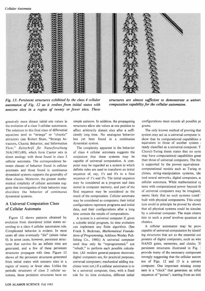
Fig

13

Persistent structures exhibited

by

the s

4

cellular

structures are almost sufficient to demonstrate

a

univers

automaton

o f

Fig. 12

as

it evolves rom nitial states with

computation capability for the cellular automaton.

nonzero sites

n

a

region

of

twenty or fewer sites.

hese

gressively more distant initial site values in

the evolution of a class 3 cellular automaton.

The solutions to this final class of differential

equations tend to strange or chaotic

attractors (see Robert Shaw, Strange At-

tractors, Chaotic Behavior, and Information

Flow,

Zeitschrift fur Naturforschung

36A(198 ):8O), which form Cantor sets in

direct analogy with those found in class 3

cellular automata. The correspondence be-

tween classes of behavior found in cellular

automata and those found in continuous

dynamical systems supports the generality of

these classes. Moreover, the greater mathe-

matical simplicity of cellular automata sug-

gests that investigation of their behavior may

elucidate the behavior of continuous

dynarnical systems.

Universal Computation Class

o

Cellular utomata

Figure 12 shows patterns obtained by

evolution from disordered initial states ac-

cording to a class

4

cellular automaton rule.

Complicated behavior is evident. In most

cases

all sites eventually die (attain value

0). In some cases, however, persistent struc-

tures that survive for an infinite time are

generated, and a few of these persistent

structures propagate with time. Figure 3

shows all the persistent structures generated

from initial states with nonzero sites in a

region of twenty or fewer sites. Unlike the

periodic structures of class 2 cellular au-

tomata, these persistent structures have no

simple patterns.

In

addition, the propagating

structures allow site values at one position to

affect arbitrarily distant sites after a suffi-

ciently long time. No analogous behavior

has yet been found in a continuous

dynamical system.

The complexity apparent in the behavior

of class cellular automata suggests the

conjecture that these systems may be

capable of universal computation. A com-

puter may be regarded as a system in which

definite rules are used to transform an initial

sequence of, say, 1's and 0's to a final

sequence of 1's and 0%. The initial sequence

may be considered as a program and data

stored in computer memory, and part of the

final sequence may be considered as the

result of the computation. Cellular automata

may be considered as computers; their initial

configurations represent programs and initial

data, and their configurations after a long

time contain the results of computations.

A system is a universal computer if, givm

a suitable initial program, its time evolution

can implement any finite algorithm.

See

Frank S. Beckman,

Mathematical Founda-

tions

of

Programming

Addison-Wesley Pub-

lishing Co., 1980.) A universal computer

need thus only be 'creprogra~med, not

rebuilt, to perform each possible calcula-

tion. (All modem general-purpose electronic

digital computers are, for practical purposes,

universal computers; mechanical adding ma-

chines were not.) If a cellular automaton is to

be a universal computer, then, with a fixed

rule for its time evolution, different initial

configurations must encode all possible pr

grams.

The only known method of proving that

system may act as a universal computer is

show that its computational capabilities a

equivalent to those of another system a

ready classified as a universal computer. T

Church-Turing thesis states that no syste

may have computational capabilities great

than those of universal computers. The thes

is supported by the proven equivalence

computational models such as Turing m

chines, string-manipulation systems, idea

ized neural networks, digital computers, an

cellular automata. While mathematical sy

tems with computational power beyond th

of universal computers may be imagined,

seems likely that no such systems could b

built with physical components. This conje

ture could in principle

be proved by showin

that all physical systems could be simulate

by a universal computer. The main obstru

tion to such a proof involves quantum m

chanics.

A

cellular automaton may be prove

capable of universal computation by identif

ing structures that act as the essential com

ponents of digital computers, such as wire

NAND gates, memories, and clocks. Th

persistent structures illustrated in Fig. 1

provide many of the necessary componen

strongly suggesting that the cellular autom

ton of Figs. 12 and 13 is a univers

computer. One important missing comp

nent is a clock that generates an h f i i t

sequence of pulses ; starting from

an

initi




configuration containing a finite number of

nonzero sites, such a structure would give

rise to an ev er-increasing numb er of nonzero

sites. If such a structure exists, it can un-

doubtedly be found by careful investigation,

although it is probably too large to be found

by any practical exhaustive search. If the

cellular autom aton of Figs. 12 and 13 is

indeed capable of universal computation,

then, despite its very simple construction, it

is in some sense capable of arbitrarily com-

plicated behavior.

Several complicated cellular automata

have been proved capable of universal com-

putation. one-dimen sional cellular auto m-

aton with eighteen possible values at each

site (and nearest neighbor interactions) has

been shown equivalent t o the simplest known

universal Turing machine. In two dimensions

several cellular automata with just two states

per site and interactions between nearest

neighbor sites (including diagonally adjacent

sites, giving a nine-site neighborhood) are

known to be equivalent to universal digital

computers. The best known of these cellular

autom ata is the Gam e of Life invented by

Conway in the early 1970s and simulated

extensively ever since. (See Elwyn R.

Berlekamp, John H. Conway, and Richard

K. Guy, Winning Ways, Academic Press,

1982 and Martin G ardner, Wheels, Life, a nd

Other Mathematical Amusements,

W.

H

Freeman and Company, October 1983.

The Life rule takes a site to have value 1 if

three an d only three of its eight neighbors a re

1 or if four are 1 and the site itself was 1 on

the previous time step.) Structures analogous

to those of Fig. 13 have been identified in the

Game of Life. In addition, a clock structure,

dubbed the glider gun, was found after a long

search.

By definition, any un iversal computer m ay

in principle be simulated by any other uni-

versal computer. Th e simulation proceeds by

emulating the elementary operations in the

first universal computer by sets of operations

in the second universal computer, as in an

interpreter program . The simulation is in

general only faster or slower by a fixed finite

factor, independent of the size or duration of

a computation. Thus the behavior of a uni-

versal computer given particular input may

be determined only in a time of the same

order as the time required to run that

universal computer explicitly. In general the

behavior of a universal computer cannot be

predicted and can be determined only by a

procedure equivalent to observing the univer-

sal computer itself.

If class 4 cellular automata are indeed

universal computers, then their behavior

may be considered completely unpredictable.

For class 3 cellular automata the values of

particular sites after a long time depend on

an ever-increa sing num ber of initial sites. Fo r

class 4

cellular automata this dependence is

by an algorithm of arbitrary complexity, and

the values of the sites can essentially be

found only by explicit observation of the

cellular automaton evolution. The apparent

unpredictability of class 4 cellular autom ata

introduces a new level of uncertainty into the

behavior of natural systems.

The unpredictability of universal com-

puter behavior implies that propositions con-

cerning the limiting behavior of universal

computers at indefinitely large times are

formally undecidable. For example, it is

undecidable whether a particular universal

computer, given particular input data, will

reach a special halt state after a finite time

or will continue its computation forever.

Explicit simulations can be run only for finite

times and thus cannot determine such infinite

time behavior. Results may be obtained for

some special input data, but no general

(finie) algorithm or procedure may even in

principle be given. If class 4 cellular autom-

ata are indeed universal computers, then it is

undecidable (in general) whether a particular

initial sta te will ultima tely evolve to the null

configuration (in which ll sites have value 0)

or will generate persistent structures. As is

typical for such generally undecidable

propositions, particular cases may be de-

cided. In fact, the halting of the cellular

automaton of Figs. 12 and 13 for

all

initial

states with nonzero sites in a region of

twenty sites has been determined by explicit

simulation. In general, the halting prob-

ability, or fraction of initial configurations

ultimately evolving to the null configuration,

is a noncomputable number. However, the

explicit results for small initial patterns sug-

gest that for the cellular automaton of Figs.

12 and 13, this halting probability is approx-

imately 0.93.

In

an infinite disordered configuration all

possible sequences of site values appear at

some point, albeit perhaps with very small

probability. Each of these sequences may be

considered to represent a possible pro-

gram ; thus with an infmite disordered initial

state, a class 4 automaton may be con-

sidered to execute (in parallel)

all

possible

programs. Program s that generate structures

of arbitrarily great complexity occur, at least

with indefinitely small probabilities. Thus,

for example, somewhere on the i n f i t e line a

sequence that evolves to a self-reproducing

structure should occur. After a suffici

long time this configuration may repro

many times, so that it ultimately domin

the behavior of the cellular automaton. E

though the prio ri probabililty for

occurrence of a self-reproducing structur

the initial state is very small, its a poste

probability after many time steps of cel

automaton evolution may be very large.

possibility that arbitrarily complex beha

seeded by features of the initial state

occur in class 4 cellular automata

indefinitely low probability prevents the

ing of meaningful statistical averages

infinite volume (length). It also suggests

in some sense any class 4 cellular autom

with an infinite disordered initial state

microcosm of the universe.

In extensive samples of cellular autom

rules, it is found that as k and r incre

class 3 behavior becomes progressively m

dominant. Class

4

behavior occur s only

2 or r 1; it becomes more common

larger

k

and but remains at the few per

level. The fact that class 4 cellular autom

exist with only three values per site

nearest neighbor interactions implies tha

threshold in complexity of construc

necessary to allow arbitrarily com

behavior is very low. However, even am

systems of more complex construction,

a small fraction appear capable of arbitr

complex behavior. This suggests that s

physical systems may be characterized

capability for class

4

behavior and unive

computation; it is the evolution of

systems that may be responsible for

complex structures found in nature.

The possibility for universal computa

in cellular automata implies that arbit

compu tations may in principle be perfor

by cellular automata. This suggests

cellular automata could be used as pract

parallel-processing computers. The m

anisms for information processing foun

most natural systems (with the exceptio

those, for example, in molecular gene

appear closer to those of cellular autom

than to those of Turing machines or con

tional serial-processing digital compu

Thus one may suppose that many nat

systems could be simulated more efficie

by cellular automata than by conventi

c o m p u t e r s . I n p r a c t i c a l t e r m s

homogeneity of cellular automata lead

simple implementation by integrated circ

A simple one-dimensional universal cell

automaton with perhaps a million sites an

time step as short as a billionth of a sec

could perhaps be fabricated with cur

Fall 983 LOS ALAMOS SCIEN



Cellular A utomata

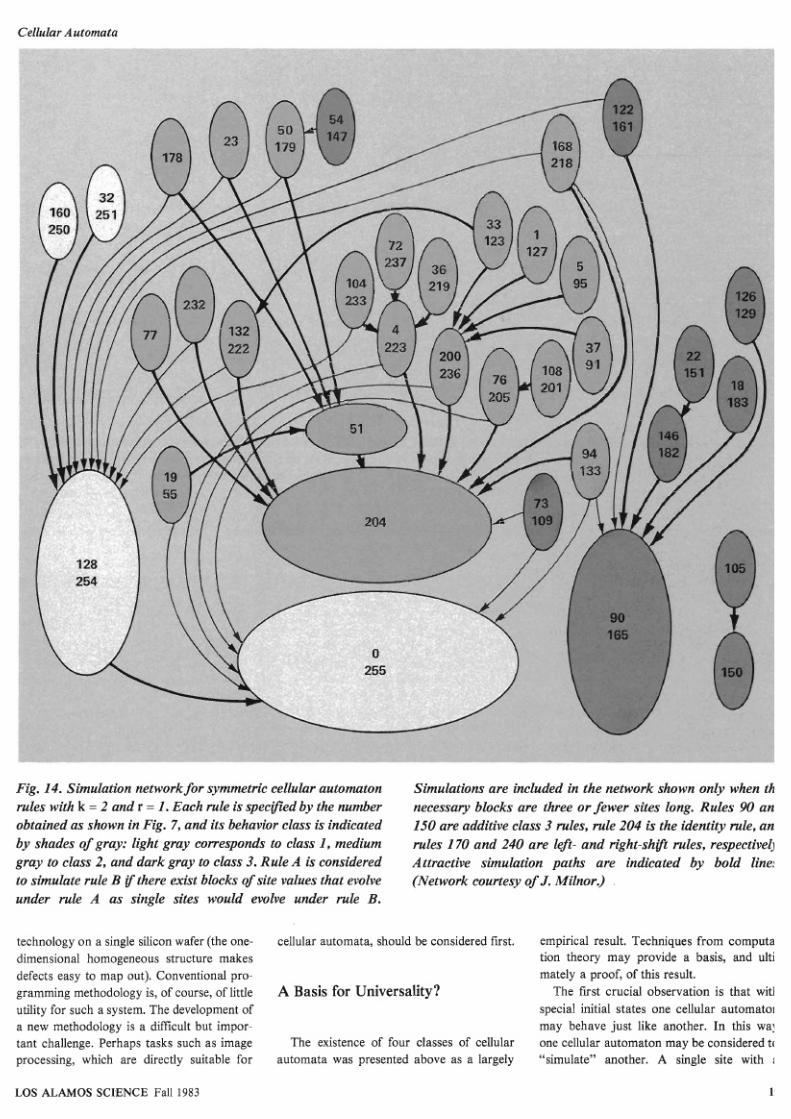
Fig. 14.

simulation

network for symmetric- b automaton os now Included zh thenetwork shown only when ti

rules with k = and r 1.Each rule is specified by the number

necessary blocks are three or fewer sites long. Rules 90 an

obtained as shown in Fig. 7,and its behavior class s indicated

15 are additive class

3

rules, rule 2 4 s the identity

rule

an

by shades of gray: light gray corresponds

to

class

1,

medium

rules 17 and 24 are left- and right-shift rules, respectively

gray

to

class

2,

and dark gray

to

class

3.

Rule A s considered Attractive simulation paths are indicated by bold lines

to simulate rule i f there exist blocks o f site values that evolve

Network courtesy

o

J . Milnor.)

under rule A as single sites would evolve under rule B.

technology on a single silicon wafer (the one-

dimensional homogeneous structure makes

defects easy to map out). Conventional pro-

gramming methodology is, of course, of little

utility for such a system. The development of

a new methodology is a difficult but impor-

tant challenge. Perhaps tasks such as image

processing, which are directly suitable for

asis for universality

cellular automata, shouldbe considered first, empirical result. Techniques trom computa

tion theory may provide a basis,

and

ulti

mately a proof, of this result.

The first crucial observation is that

with

special initial states one cellular automaton

may behave just like another. In this way

The existence of four classes of cellular

one cellular automaton may be considered to

automata was presented above s a largely

simulate another. single site with

LOS L MOS SCIENCE Fall 983



particular value in one cellular automaton

may be simulated by a fixed block of sites in

another; after a fixed number of time steps,

the evolution of these blocks imitates the

single time-step evolution of sites

in

the first

cellular automaton. For example, sites with

value 0 and 1 in th e first cellular automaton

may be simulated by blocks of sites 00 and

11, respectively,

in

the second cellular

automaton, and two time steps of evolution

in

the second cellular automaton correspond

to one time step in the first. Then, with a

special initial state c ontaining 1 1 and 00 but

not 0 1 and 10 blocks, the second cellular

automaton may simulate the first.

Figure 14 gives the network that repre-

sents the simulation capabilities of sym-

metric cellular automata with k 2 and r

1. (Only simulations involving blocks of

length less than four sites were included in

the constructio n of the network.) If a cellular

automaton is computationally universal,

then with a su fficiently long encoding it

should be able to simulate any other cellular

automaton, so that a path should exist from

the node that represents its rule to nodes

representing

all

other possible rules.

n example of the simulation of one

cellular automaton by another is the simula-

tion of the additive rule 90

Eq.

1) by the

class rule 18.

A

rule 18 cellular automaton

behaves exactly like a rule 90 cellular

automaton if alternate sites in the initial

configuration have value 0 (so that 0 and 1

in

rule 90 are represented by 00 and 01

in

rule 18) and alternate time steps are con-

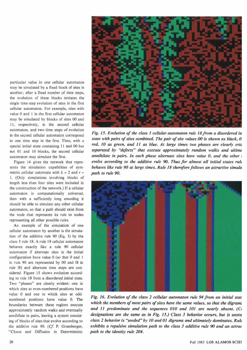
sidered. Figure 15 shows evolution accord-

ing to rule 18 from a disordered initial state.

Two phases are clearly evident: one in

which sites at even-numbered positions have

value 0 and one in which sites at odd-

numbered positions have value 0. The

boundaries between these regions execute

approxim ately rando m w alks and eventually

annihilate in pairs, leaving a system consist-

ing of blocks of sites that evolve according to

the additive rule 90.

Cf.

Grassberger,

Chaos and Diffusion in Deterministic

Fig.

15.

Evolution of the class

3

cellular automaton rule

18

rom a disordered in

state with pairs of sites combined. The pair of site values

00

is shown as black, 01

red, 10 as green, and 11 as blue. At large times two phases are clearly evid

separated by defects'' that execute approximately random walks and ultima

annihilate in pairs. In each phase alternate sites have value

0

and the other s

evolve according to the additive rule

90

Thus for almost all initial states rule

behaves like rule 90 at large times. Rule 18 therefore ollows an attractive simula

path to rule

90.

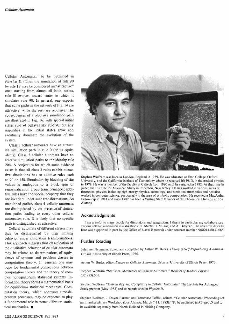
Fig. 16.Evolution of the class 2 cellular automaton rule 9 from

an

initial state

whi h the members o f most pairs of sites have the same values, so that the digrams

and 11 predominate and the sequences 010 and 101 are nearly absent. (Co

designations are the same as

in

Fig. 15.) Class

3

behavior occurs, but

s

unsta

class 2 behavior is seeded by 10and 01 digrams and ultimately dominates. Rule

exhibits a repulsive simulation path

to

the class

3

additive rule

90

and an attrac

path to the identity

rul 204.

Fall 983

LOS

ALAMOS

S IE



Cellular utomata

worked in computer science patitadarly

in

the re

of

sym olic

computation

Be recaV9ft MacArtbur

Fellowship in

98

and since 982 h s been a Visiting taff Member of theTheoretical ivision t Los

Acknowledgments

Ithank

v a r i i ~ ~ellular

astf-mwn

t w aai

here auwrted in

OF

^Navd

~ s~ssehQWeg r ~g b0 ^ 1 4 4 ~

Stephen Wolfram,

J.

Doyne Farmer, and Tomm aso Toffoli, editors. Cellular Autom ata: Proceedings o

an Interdisciplinary Workshop (Lo s A larnos; March7-1

1

1983). To

be

published in Physica and to

be available separately from North-Holland Publishing Company.



HISTORIC L

PERSPECTIVE

rom

T u h g

and

von Neumann

t

the

Present



HISTORIC L

PERSPECTIV



we11 organized that as soon as an error

shows up in any one part of it, the system

automatically senses whether this error m at-

ters Qr not. If it doesn't matter, the system

continues to operate without paying any

attention to it. If the error seems to be

impo rtant, the system blocks that region out,

by-passes it a nd proceeds along other chan-

nels. ?'he system then andyzes the region

separately at leisure and corrects what goes

on there, and if correction is impossible the

system just blocks the region off and by-

passes it forever.

To apply the philosophy underlying

natural automata to artificial automata we

must understand complicated mechanisms

better than we do, we must have elaborate

statistics about what goes wrong,

nd

we

must have much more perfect statistical

information about the milieu in which a

mechanism lives than we now have. An

automaton cannot be separated from the

milieu to which it responds

(ibid.,

pp

\,

\ \

71-72). \ / \ 1

From ar tZ cid autom ata one gets a ve

strong impression that complication, or

reductive potentiality in an organization9 s

egenerative, that an organization which

synthesizes something is necessarily more

d, of a higher order, than the

ation it synthesizes

ibid.,

p. 79).

defeats degeneracy. Although the

mplicated aggregation of many elemmtwy

rts necessary to form a living organism is

ermodynamicd4y highly improbable, once

such a peculiar accident occurs, the

rules

of

probability do not apply because the or-

ganism can reproduce itself provided the

milieu is reasonable-and a reasonab le

milieu is thermodynamically much less h-

probable. Thus probability leaves a loophole

at is pierced by self-reproduction.

Is it possible for

an

artscial automaton to

reproduce itself? Further, is it possible fo r a

machine to produce something that is more

complicated

th n

its&

in

the sense that the

offspring can perform more dMcult and

involved tasks than the progenitor? These

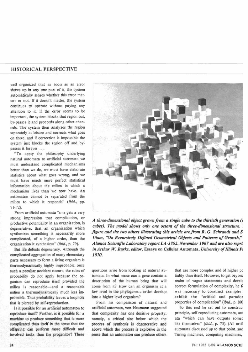
A three-dimemiom1 object grown from a sirzgle cube to the thirtieth generation d

cubes).

The

w & l shows od y one oc- cf the three-dimnswml structure*

figure and the

wu

others illustrating this

urticle

arefrom

Re

. Schrandt and

S

h On

Recursive&

D&ed

Geometrical Objects and Patterns of Growth,

A l m o s Scien@c &&oratory re p rt L 3762 November

1 7

re u&o

repri

in

Arthur

W

w h , editor, ssays

on Cellular Automata

Udversi@o i'llinois Pr

1970



HISTORICAL PERSPECTIVE

neighborhood consisting of the four cells

orthogonal to it. Influenced by the work of

McCulloch and Pitts, von Neumann used a

physiological simile of idealized neurons

to

help define these states. The states and

transition rules among them were designed

to perform both logical and growth opera-

tions. He recognized, of course, that his

construction might not be the minimal or

optimal one, and it was later shown by

Edwin Roger Banks that a universal self-

reproducing automaton was possible with

only four allowed states per cell.

The logical trick employed to make the

automaton universal was to make it capable

of reading any axiomatic description of any

other automaton, including itself, and to

include its own axiomatic description in its

memory. This trick was close to that used by

Turing in his universal computing machine.

The basic organs of the automaton included

a tape unit that could store information on

and read from an indefinitely extendible

linear array of cells, or tape, and a construct-

ing unit containing a finite control unit and

an indefinitely long constructing arm that

could construct any automaton whose de-

scription was stored in the tape unit. Realiza-

tion of th e 29-state self-reproducing cellular

automaton required some 200,000 cells.

Von Neum ann died in 1957 and did not

complete this con struction (it was com pleted

by Arthur Burks). Neither did he complete

his plans for two other models of self-

reproducing automata. In one, based on the

29-state cellular automaton, the basic ele-

ment was to be neuron-like and have fatigue

mechanisms

as

well a s a threshold for exc ita-

tion.

The

other was to be a continuous model

of

self-reproduction described by

a

system of

nonlinear partial differential equations of the

type that govern diffusion in a fluid. Von

Neumann thus hoped to proceed from the

discrete to the continuous. He was inspired

by the abilities of natural automata and

emphasized that the nervous system was not

purely digital but was a mixed analog-digital

system.

Much effort since von Neumann's time

has gone into investigating the simulation

capabilities of cellular automata. Can one

define appropriate sets of states and transi-

tion rules to simulate natural phenomena?

Ulam was among the first to use cellular

automata in this way. He investigated

growth patterns of simple finie systems,

simple in tha t each cell had only two sta tes

and obeyed some simple transition rule.

Even very simple growth rules may yield

highly complex patterns, both periodic said

aperiodic. "The main feature of cellular

automata," Ulam points out, is that simple

recipes repeated many times may lead to

very complicated behavior. Information

analysts might look at some final pattern said

infer that it contains a large amount of

information, when in fact the pattern is

generated by a very simple process. Perhaps

the behavior of an animal or even ourselves

could be reduced to two or three pages of

simple rules applied in turn many times "

(private conversation, October 1983).

Ulam's study of the growth patterns of

cellular autom ata had as on e of

its

aims "to

throw a sidelight on the question of how

much 'information' is necessary to describe

the seemingly enormously elaborate struc-

tures of living objects"

ibid.).

His work with

Holladay and with Schrandt on

an electronic

computing machine at Los Alamos

in

1967

produced a great number of such patterns.

Properties of their morphology were

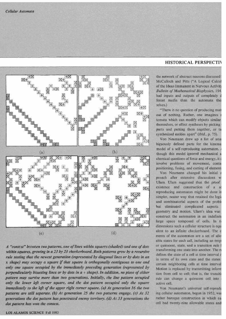
surveyed in both space and time. U l m and

Schrandt experimented

wit

"contests" in

which tw o s tarting configurations were al-

lowed to grow until

they collided. Then

a

fight would ensue,

and

sometimes one con-

figuration would annihilate the other. They

also explored three-dimensional automa ta.

Another early investigator of cellular

automata was Ed Fredkin. Around 1960he

beg n

to explore the possibility that all

physical phenomena down to the quantum

mechanical level could be simulated by

cellular automata. Perhaps the physical

world is a discrete space-time lattice of

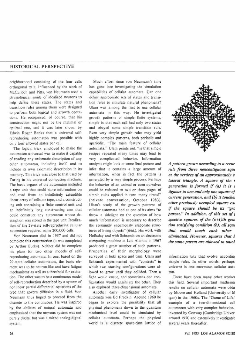
A pattern grown

according

to a ecurs

rule

from three

noncontigwus squa

at the vertices

o f an

approximately

eq

lateral triangle. A square of the n

generation

is

formed i a) U is c

tiguous

to

one nd

only

one square

o f

current

generation

nd

b)

it

touches

otherpreviously occupied

square

exc

the

square

should be its

* gra

parent In addition, of Ms set c f p

spective squecres qf the w-l)th

gene

tion 5~atvtfyws

ondition

@ dll squa

that would touch each

other

eliminated However, squares that h

the someparent

are allowedto

ouch

information bits that evolve according

simple

rules.

In

other

words,

universe is one enormous cellular anto

ton.

There have

been

many other worker

this field. Several

important mathemati

results OB cellular automata were obtai

by Moore and Holland (University of M

igan) in the 1960s

The Gases

of Life,

example of a two-dimensional cell

automaton with

very

complex behavior

invented by Conway CambridgeUniversi

around 1970 and extensively investigated

several

years

thereafter.



Cellular utomata

HISTORICAL PERSPECTIV

Cellular automata have been used in bio-

logical studies (sometimes under the names

of tesselation automata or b'hornogeneous

structures ) to model several aspects of the

growth and behavior of organisms. They

have been analyzed as parallel-processing

com puters (often under the name of iter-

ative arrays ). They have also been applied

to problems in number theory under the

name stunted trees and have been con-

sidered

in

ergodic theory, as endomorphisms

of

the

dynarnical shift system.

A workshop on cellular automata at Los

Alamos

in

March 1983 was attended by

researchers from many different fields.

The

proceedings of this workshop will be pub-

lished in the journal Physica

D said

will

also

be issued as a book by North-Holland

Publishing Co.

In all this effort the work of Stephen

Wolfram most closely approa ches von Neu-

mann's dream of abstracting from examples

of complicated au tomata new concepts rele-

vant to information theory and analogous to

the concepts of thermodynamics. Wolfram

has made a systematic study of one-dimen-

sional cellular automata and has identified

four general classes of behavior, as described

in the preceding article.

Three

of

these classes exhibit behavior

analogous to the limit points, limit cycles,

and strange attractors found in studies of

nonlinear ordinary differential equations and

transformation iterations. Such equations

characterize dissipative systems, sys tems in

which structure may arise spontaneously

even from a disordered initial state. Fluids

and living organisms are examples of such

systems. (Non-dissipative systems, in con-

trast, tend toward disordered states of max-

imal entropy and are described by the laws

of thermodynamics.) T he fourth class mim-

ics the behavior of universal Turing ma-

chines. Wolfram speculates that his identifi-

cation of universal classes of behavior in

cellular automata may represent a first step

in the formulation of general laws for com

plex self-organizing systems. He says tha

what he is looking for is a new con

cept-maybe it will be complexity or mayb

something else-that like entropy will b

always increasing (or decreasing) in such

system and will be manifest in both th

microscop ic laws governing evolution of th

system and in its macroscopic behavior.

may be closest to what von Neumann had i

mind as he sought a correct definition o

complexity. We can never know. We ca

only wish Wolfram luck in finding it. rn

Acknowledgment

I wish to thank Arthur

W.

Burks for pe

mission to reprint quotations from

heory

o

Self Reproducing

A utomata. We ar

indebted to him for editing and completin

von Neumann's manuscripts in a manne

that retains the patterns of thought of a grea

mind.

Further Reading

John von Neumann.Theory of

Self-Reproducing

Automata.

Edited

and completed

by Arthur W.

Bwks.

Urbana: University

of

Illinois

Press

1966.

Part s an

edited version of the le tures

delivered

at the

University of Illinois. Part I1 is von Neumann's

manuscript

describing the construction of his 29-state

self-reproducing automaton.

Arthur

W

urks, editor.

Essays

on ellular

Automata. Urbaaa: University

of

Illinois Press, 1970.

This

volume contains early

papers

on cellular automata including those of Ulam and his coworkers.

Aadrew

~ d g e s Aten Turing:Mathematician

and

Computer

Bailder. ;Ww

Scienriis~,15 Septmber

1963,

pp 789-792.

This

contains

a

wonderful

illustration, A

Turing

Machine inAction.

Martin

Gardner. On CellularAutomata, Sdf-Reproduction, the Garden

of

Eden,

and

the

G m e

We.

Scientific American October 1971.

The following publicationsdeal with

complexity

per

se:

W

A.

Beyer M

L. Stein, and

6

M

Ulm

The

Notiua

of Compterity.

Los

Aiaaos Stae aic

Laboratory

report

LA-4822,

ecember 1971.

Wolfram Automata

Documents

Transcript of Wolfram Automata