A Web-Based RPi PicoPak Monitor

W.J. RileyHamilton Technical Services

Beaufort, SC 29907 USAbill@wriley.com

Introduction

This paper describes a web-based application to monitor a PicoPak [1] or PicoPlus [2] clockmeasurement on a Raspberry Pi computer [3]. It is an alternative to the PicoMon program [4] when aPicoPak PostgreSQL database [5] is not available. The rpimon PHP script (shown in Appendix I) islaunched from a web browser (e.g., Firefox [6]) to display a plot of the current phase or frequency data.

Description

A PicoPak or PicoPlus clock measurement module can be run by a small and inexpensive Raspberry Picomputer running a Python script [7]. The RPi can be operated remotely using putty [8] via a SSHconnection [9] without needing a monitor, keyboard or mouse. The resulting data can be stored in atmpfs shared memory RAM file [10] on the RPi and accessed remotely from a Windows workstationusing WinSCP [11] or another such application. During a measurement, it is desirable to be able tomonitor the progress of the run. A plot of the phase or frequency data is an effective way of doing that,particularly via a WiFi or Ethernet LAN connection using an ordinary web browser. That is thepurpose of the rpimon program described herein. Examples of phase and frequency plots for a smalldata set are shown in Figures 1 and 2 respectively. The plots show either scaled phase in seconds ordimensionless fractional frequency as a function of time as indicated by a (possibly-averaged) datapoint number. The measurement tau is always 1 second, and the displayed data are therefore for anaveraging time in seconds equal to the averaging factor. Frequency offset and Allan deviation valuesare shown for the averaged data, and the span of the data is shown as beginning and end MJD timetags.Lines denote the linear slope of the phase data or average of the frequency data.

RPiMon Commands

Examples of rpimon web browser command lines for phase and frequency plots are as follows:

192.168.2.15/rpimon.php192.168.2.15/rpimon.php?type=phase&af=10192.168.2.15/rpimon.php?type=freq&af=0

The numeric (dot) IP address for the RPi is followed by the rpimon.php script name and two optionalarguments that set the data plot type (phase or freq) and the averaging factor (af). Without thesearguments, the script defaults to a phase plot with automatic averaging. The RPi IP address can befound via SSH with the command hostname -I. An af=0 tells the program to use an automatically-determined averaging factor (set by the program macro MAXSIZE). The averaging factor will be thesmallest value that results in less than MAXSIZE plot points. An af=1 disables averaging, while anaf>1 denotes the averaging factor to be used. The span of the data (in days) is the difference betweenthe two MJD values shown on the x-axis of the plot. Desktop shortcuts can be created for the tworpimon commands to support PicoPak/Plus monitoring with a mouse click.

Figure 1. PicoPak/Plus RPi Web Monitor Phase Data Plot

Figure 2. PicoPak/Plus RPi Web Monitor Frequency Data Plot

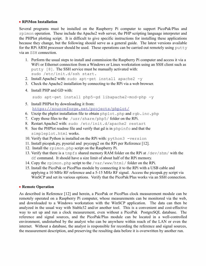
RPiMon Installation

Several programs must be installed on the Raspberry Pi computer to support PicoPak/Plus andrpimon operation. These include the Apache2 web server, the PHP scripting language interpreter andthe PHPlot plotting script. It is difficult to give specific instructions for installing these applicationsbecause they change, but the following should serve as a general guide. The latest versions availablefor the RPi ARM processor should be used. These operations can be carried out remotely using puttyvia an SSH connection.

1. Perform the usual steps to install and commission the Raspberry Pi computer and access it via a WiFi or Ethernet connection from a Windows or Linux workstation using an SSH client such asputty [8]. The SSH service must be manually activated with:sudo /etc/init.d/ssh start.

2. Install Apache2 with: sudo apt-get install apache2 -y3. Check the Apache2 installation by connecting to the RPi via a web browser.

4. Install PHP and GD with:

sudo apt-get install php5-gd libapache2-mod-php -y

5. Install PHPlot by downloading it from: https://sourceforge.net/projects/phplot/

6. Unzip the phplot installation file to obtain phplot.php and rgb.inc.php7. Copy those files to the /usr/share/php5/ folder on the RPi. 8. Restart Apache2 with: sudo /etc/init.d/apache2 restart9. See the PHPlot readme file and verify that gd is in phpinfo and that the

simpleplot.html works.10. Verify that Python is installed on the RPi with: python3 -version11. Install picopak.py, pyserial and psycopg2 on the RPi per Reference [12].12. Install the rpimon.php script on the Raspberry Pi.13. Verify that there is a tmpfs shared memory RAM folder on the RPi at /dev/shm/ with the

df command. It should have a size limit of about half of the RPi memory.14. Copy the rpimon.php script to the /var/www/html/ folder on the RPi.15. Install the PicoPak or PicoPlus module by connecting it to the RPi with a USB cable and

applying a 10 MHz RF reference and a 5-15 MHz RF signal. Access the picopak.py script via WinSCP and set its various options. Verify that the PicoPak/Plus works via an SSH connection.

Remote Operation

As described in Reference [12] and herein, a PicoPak or PicoPlus clock measurement module can beremotely operated on a Raspberry Pi computer, whose measurements can be monitored via the web,and downloaded to a Windows workstation with the WinSCP application. The data can then beanalyzed in the usual way with Stable32 and/or another tool. This is a convenient and cost-effectiveway to set up and run a clock measurement, even without a PicoPak PostgreSQL database. Thereference and signal sources, and the PicoPak/Plus module can be located in a well-controlledenvironment, undisturbed by the analyst who can be anywhere within reach of the LAN or even theinternet. Without a database, the analyst is responsible for recording the reference and signal sources,the measurement description, and preserving the resulting data before it is overwritten by another run.

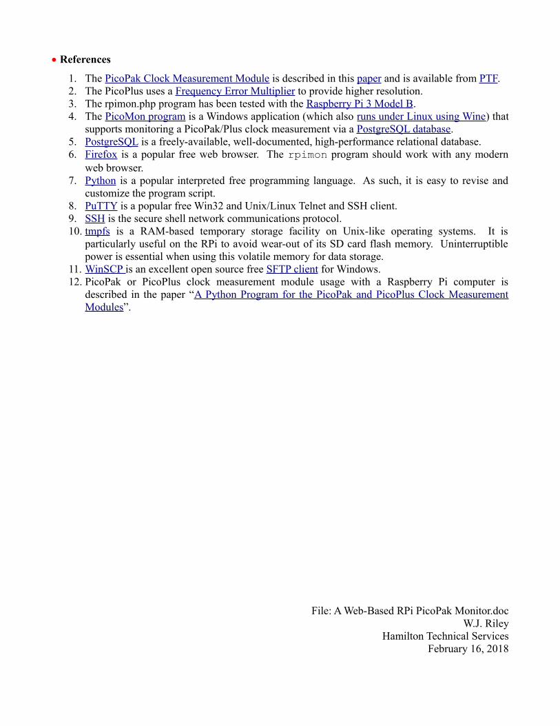
References

1. The PicoPak Clock Measurement Module is described in this paper and is available from PTF.2. The PicoPlus uses a Frequency Error Multiplier to provide higher resolution.3. The rpimon.php program has been tested with the Raspberry Pi 3 Model B.4. The PicoMon program is a Windows application (which also runs under Linux using Wine) that

supports monitoring a PicoPak/Plus clock measurement via a PostgreSQL database.5. PostgreSQL is a freely-available, well-documented, high-performance relational database.6. Firefox is a popular free web browser. The rpimon program should work with any modern

web browser.7. Python is a popular interpreted free programming language. As such, it is easy to revise and

customize the program script. 8. PuTTY is a popular free Win32 and Unix/Linux Telnet and SSH client.9. SSH is the secure shell network communications protocol.10. tmpfs is a RAM-based temporary storage facility on Unix-like operating systems. It is

particularly useful on the RPi to avoid wear-out of its SD card flash memory. Uninterruptiblepower is essential when using this volatile memory for data storage.

11. WinSCP is an excellent open source free SFTP client for Windows. 12. PicoPak or PicoPlus clock measurement module usage with a Raspberry Pi computer is

described in the paper “A Python Program for the PicoPak and PicoPlus Clock MeasurementModules”.

File: A Web-Based RPi PicoPak Monitor.docW.J. Riley

Hamilton Technical ServicesFebruary 16, 2018

Appendix Irpimon.php Program Listing

<?php# ----------------------------------------------------------------------------# RPiMon PicoPak/Plus Web Monitor Script rpimon.php# to display phase or frequency data during a PicoPak/Plus measurement# ----------------------------------------------------------------------------## Rev 0 02/10/18 Created from picomon_img.php# 02/13/18 Adapted for use with RPi without a database# 02/14/18 Basically working# Revising, refining and debugging# This script works nicely by itself with type & af args# 02/15/18 This script works OK on RPi# Revise so no plot type and/or AF entry required# Change name to rpimon.php (after saving original# rpimon.php as rpimon.php.bak2)# 02/16/18 Remove some testing code# Made filename a macro## (c) 2018 W.J. Riley Hamilton Technical Services All Rights Reserved# Released under the MIT license which allows unrestricted# free use by anyone for any purpose. E-Mail: bill@wriley.com# ----------------------------------------------------------------------------# This RPi PicoPak/Plus web monitor works without a PostgreSQL database.# It can be called by itself or via rpimon.php.# The data filename must be entered manually into this script.# The data tau is fixed at 1 second.# The measurement start and end (current) MJDs are read from the data file.# The PicoPak/Plus type and S/N are not known by this script.# The signal and reference source IDs and names are not known by this script.# The measurement description is not known by this script.# ----------------------------------------------------------------------------# This rpimon.php script can be called with or without phase and af# arguments. For example:# rpimon.php?type=phase&af=0 will plot the phase data with default AF# rpimon.php without arguments will also plot the phase data with default AF# rpimon.php?type=freq&af=0 will plot the frequency data with default AF# rpimon.php?type=phase&af=1 will plot all the phase data# rpimon.php?type=freq&af=1 will plot all the frequency data# rpimon.php?type=phase&af=100 will plot the phase data with AF=100# rpimon.php?type=freq&af=100 will plot the frequency data with AF=100# ----------------------------------------------------------------------------# Functions:# read_data()# read_and_downsample_data()# calc_freq_slope()# calc_freq_avg()# calc_sigma()# phase_to_freq()# scale_phase_data()# scale_freq_data()# get_current_mjd()# calc_span() // Not used# draw_graph()# ----------------------------------------------------------------------------# This PHP script generates a phase or frequency data plot using PHPlot.# ----------------------------------------------------------------------------

# Some comments re the # of data points and data array size:# At some point (say 10k) the # of points in a plot reaches# a value where more doesn't add insight, especially for a# frequency plot where it often becomes just a solid band of noise.# There are also issues of speed and resource limits.# In fact, there appears to be some problem with PHP/PHPlot with# data sets greater than around 100k points, a number easily exceeded# by 1 second PicoPak/Plus data over longer than a day.# So some sort of data averaging/decimation/downsampling is needed.# Downsampling is easy to do with phase data,# and that is what is done here. In fact, it's quite easy to do# since the entire data set is read from the data file# and then put into a plot array of arrays for plotting.# One can either bound the # of points with an averaging factor# or set a "even" one. The former seems best for an automated process,# while the later may be preferred for manual analysis.# Either is supported, and macros allow their choice here. The AF and# statistics are shown in a legend, calculated for the averaged data.# The user can enter the AF on rpimon.php command line# and pass it to this image script on its command line# If AF=0 => Do avergaing using default MAXSIZE# If AF=1 => No averaging, use all data# If AF>1 => Do averaging by user-chosen factor## Notes for rpimon.php:# The only URL parameters are type and af# We get the begin_mjd, end_mjd and # points from the data file# The # points is estimated from the size of the data file# The tau is always 1 second and the plot size is fixed# We don't know and don't display the module type or S/N# We don't know and don't displat the signal and reference source IDs# We don't know and don't display a measurement description# The data tau is fixed at 1 second. It would be possible to# determine it from the MJD timetags, perhaps by their span# divided by the # of points, rounded to the closest integer seconds

require_once 'phplot.php';

# Data filenamedefine('FILENAME', "/dev/shm/picopak.dat");# Plot sizedefine('PLOT_WIDTH', 600);define('PLOT_HEIGHT', 400);# Global variables for this file# The phase array is an array of arrays# Each row has 3 items:# An empty label string '', the x value (point #)# and the phase value (which gets scaled)$phase = array(array('', 0, 0));# Also define a frequency data array of arrays$freq = array(array('', 0, 0));# Set tau to 1 second$tau = 1.0;# Get averaging factor from command lineif(!empty($_GET['af'])){

$af = intval($_GET['af']);}else // Default AF for no af entry

{ # Set af to 0 for automatic averaging

$af=0;}# If DOWNSAMPLE is TRUE# The phase data are downsampled by the averaging factor# as it is put into the $phase[][] array, so all use of# tau in this script is multiplied by $af except if# the af is zero as a code for using MAXSIZE# In that default case, AF and tau are determined later# by the data file size before it is readif($af>0){

$tau = $tau * $af;}# Set plot width in pixels$w = PLOT_WIDTH;# Set plot height in pixels$h = PLOT_HEIGHT;# Phase data units$units = " ";# Get plot type from command lineif(!empty($_GET['type'])){

if($_GET['type'] == 'freq'){

# Set plot type & title to freq$type = "freq";$title = "PicoPak Frequency Data";

}else // Default for anything else{

# Set plot type & title to phase$type = "phase";$title = "PicoPak Phase Data";

}}else // Default for no type entry{

# Set plot type & title to phase$type = "phase";$title = "PicoPak Phase Data";

}

# Set several initial values# # phase data points, N$numN = 0;# Start MJD$begin = 0.0;# End MJD$end = 0.0;# Current MJD$now_mjd = 0.0;# # freq data points, M$numM = 0;# Phase slope$slope = 0.0;# Phase intercept$intercept = 0.0;

# Average fractional frequency offset$frequency = 0.0;# Average frequency$avg = 0.0;# Raw sigma$sigma = 0.0;# Formatted ADEV$adev = 0.0;# Legends$leg1 = '';$leg2 = '';$leg3 = '';# Time$days = 0;$hours = 0;$mins = 0;$secs = 0;# Macros to control legendsdefine('SHOW_FREQ', TRUE);define('SHOW_ADEV', TRUE);# Macros to control plot linesdefine('SHOW_AVG', TRUE);define('SHOW_SLOPE', TRUE);# Macros to control downsamplingdefine('DOWNSAMPLE', TRUE);define('MAXSIZE', 5000);define('MANUAL_AF', FALSE);define('AF', 1000); // Set value for manual AF# Macro to show begin and end MJDs in plot X-Axis labeldefine('SHOW_MJDS', TRUE);

# ----------------------------------------------------------------------------# There is no check for parameters supplied to this web page.# A suitable call would be: rpimon_img.php?type=phase&af=1# ----------------------------------------------------------------------------# The following function reads all the phase data for a PicoPak or# PicoPlus module from a shared memory RAM file e.g., /dev/shm/picopak.dat.# The data file has 2 columns (MJD and phase), 1 point/line, with tau=1s.# The entire data file is read and the phase values are parsed and put into# the $phase[][] array, an array of arrays, without averaging, each of which# is a blank label string, an index, and a phase value in seconds.# The number of data points is put into $numN and $n, and the first and last# MJDs are put into $begin and $end respectively.## Function to read phase data from data file# No return (void)function read_data(){ # INPUTS // None;

# OUTPUTS GLOBAL $phase; GLOBAL $numN; GLOBAL $begin; GLOBAL $end; GLOBAL $title;

# Initialize the point index

$i = 0;

# Read phase data from file. # Open data file for reading $file = fopen(FILENAME, "r");

# Loop through entire file while (!feof($file)) {

# Read 1 line$line = fgets($file);

# Reject empty line# Note: It may have CR/LF# Actual data line must have at least 10 charactersif(strlen($line)<10){

break;}

# Explode it into two parts$data = explode(' ', $line);

# MJD is 1st part# Save 1st MJD as $beginif($i==0){

$begin = $data[0];}

# Save every MJD as $end - last one is used$end = $data[0];

# Phase value is 2nd part$phaseval = $data[1];

# Save point in $phase array for data-data plot format# The 1st item in each $phase row is a blank label# The 2nd item in each $phase row is the data point ## It starts at 1 and goes to $numN# The 3rd item in each $phase row is the phase value, s$phase[$i][0] = '';$phase[$i][1] = $i+1;$phase[$i][2] = $phaseval;

# Increment the point index $i ++; }

# Set the # points$numN = $i;$n = $i;

# Close the data filefclose($file);

# Check that we got dataif($numN==0){

# No Data# Put message into the plot title to display it$title = "No Data"; // Error

}}

# ----------------------------------------------------------------------------# The following function reads and optionally downsamples the phase data# for a PicoPak or PicoPlus module from a shared memory RAM file# e.g., /dev/shm/picopak.dat.# The data file has 2 columns (MJD and phase), 1 point/line, with tau=1s.# The entire data file is read and the phase values are parsed and put into# the $phase[][] array, an array of arrays, with optional averaging, each# of which is a blank label string, an index, and a phase value in seconds.# The number of data points is put into $numN and $n, and the first and last# MJDs are put into $begin and $end respectively.## Function to read phase data from data file# No return (void)function read_and_downsample_data(){ # INPUTS GLOBAL $af;

# OUTPUTS GLOBAL $phase; GLOBAL $numN; GLOBAL $begin; GLOBAL $end; GLOBAL $now_mjd; GLOBAL $af; GLOBAL $tau; GLOBAL $title;

# Initialize the point index and count $i = 0; $n = 0;

# Set the averaging factor if($af == 0) // Use default averaging per MAXSIZE { # Determine the required averaging factor # We don't know the # of data points # so we estimate it from the file size # There are an average of about 41 characters/line # It's not critical what the exact AF is so this is OK $numN = filesize(FILENAME); $numN /= 41; $af = ceil($numN / MAXSIZE);

# Adjust the analysis tau accordingly $tau = $tau * $af; } else { # Otherwise, use user-entered AF }

# Manually set AF per AF macro if MANUAL_AF is TRUE

if(MANUAL_AF) { $af = AF; }

# Read phase data from file. # Open data file for reading $file = fopen(FILENAME, "r");

# Loop through entire file while (!feof($file)) {

# Read 1 line$line = fgets($file);

# Reject empty line# Note: It may have CR/LF# Actual data line has at least 10 charactersif(strlen($line)<10){

break;}

# Explode it into two parts$data = explode(' ', $line);

# MJD is 1st part# Save 1st MJD as $beginif($i==0){

$begin = $data[0];}

# MJD is 1st part$now_mjd = $data[0];

# Phase value is 2nd part$phaseval = $data[1];

# Is this a downsampled point? if(($i % $af)==0) {

# Save point in $phase array for data-data plot format# The 1st item in each $phase row is a blank label# The 2nd item in each $phase row is the data point ## It starts at 1 and goes to $numN# The 3rd item in each $phase row is the phase value, s$phase[$n][0] = '';$phase[$n][1] = $n+1;$phase[$n][2] = $phaseval;

# Save every (and last) MJD$end = $data[0];

# Increment the point count$n ++;

}

# Increment the point index

# Point index $i is used for modulus calc $i ++; }

# Set the # points$numN = $n;

# Close the data filefclose($file);

# Check that we got dataif($numN==0){

# No Data# Put message into the plot title to display it$title = "No Data";

}}

# ----------------------------------------------------------------------------# Function to calculate the average frequency offset# as the slope of the linear regression of the phase data# Returns $slopefunction calc_freq_slope($phase, $tau){ # OUTPUT GLOBAL $intercept;

# Local variables for sums, slope and intercept $x = 0; $y = 0; $xy = 0; $xx = 0; $slope = 0;

# Get # phase data points $numN = count($phase);

# Accumulate sums for($i=0; $i<$numN; $i++) { $x += $i+1; $y += $phase[$i][2]; $xy += ($i+1)*$phase[$i][2]; $xx += ($i+1)*($i+1); }

# Calculate slope $slope = (($numN*$xy) - ($x*$y)) / (($numN*$xx) - ($x*$x));

# Calculate y intercept $intercept = (($y - $slope*$x) / $numN);

# Scale slope for measurement tau $slope /= $tau;

# Return slope return $slope; }

# ----------------------------------------------------------------------------# Function to calculate the average frequency offset# as the average of the freq data# Returns $avgfunction calc_freq_avg($freq){ // OUTPUT GLOBAL $avg;

# Local variable for sum $x = 0;

# Get # freq data points $numM = count($freq); # Accumulate sum for($i=0; $i<$numM; $i++) { $x += $freq[$i][2]; }

# Calculate average $avg = $x / $numM;

# Return average return $avg; }

# ----------------------------------------------------------------------------# Function to calculate the Allan deviation# for the phase data at its data tau (AF=1)# Returns $sigmafunction calc_sigma($phase, $tau){ # Local variables for sum $s = 0; $ss = 0;

# Get # data phase points $numN = count($phase);

# Accumulate sum for($i=0; $i<$numN-2; $i++) { $s = $phase[$i+2][2] - (2*$phase[$i+1][2]) + $phase[$i][2]; $ss += $s*$s; }

# Calculate ADEV $sigma = sqrt($ss / (2*($numN-2)*$tau*$tau));

# Return ADEV return $sigma;}

# ----------------------------------------------------------------------------# Function to convert phase data to frequency data# No return (void)

function phase_to_freq($phase, $freq, $tau){ // OUTPUT GLOBAL $numM; GLOBAL $freq; # Get # phase data points $numN = count($phase); # Calculate 1st differences of phase # Note: Phase and freq array indices are 0-based # but their 1st points are marked 1 in their [0][1] values # There is 1 fewer frequency data point (M=N-1) for($i=0; $i<$numN-1; $i++) { $freq[$i][0] = ''; $freq[$i][1] = $i; $freq[$i][2] = ($phase[$i+1][2]-$phase[$i][2])/$tau; }

# Get # freq data points # Their array index $i goes from 0 to numM-1 = 0 to numN-2 # and their $freq[$i][1] label goes from 1 to numm $numM = count($freq);}

# ----------------------------------------------------------------------------# The following function scales the phase data to engineering units# It takes the indexed phase data array as a parameter,# scales it to engineering units, and returns the units name# We handle s, ms, us, ns and ps# If abs data range is < 1000e-12, we use ps and scale by 1e12# If abs data range is < 1000e-9, we use ns and scale by 1e9# if abs data range is < 1000e-6, we use us and scale by 1e6# Otherwise, we use ms and scale by 1e3## Function to scale phase data to engineering units# Returns $unitsfunction scale_phase_data(){ # INPUTS GLOBAL $phase;

# OUTPUTS GLOBAL $units; GLOBAL $factor; GLOBAL $numN;

# Get # data phase points $numN = count($phase);

# Find data range (range = max - min) $max = $phase[0][2]; $min = $max; # Find max and min of phase data for($i=0; $i<$numN; $i++) { # Find max

if($phase[$i][2] > $max) { $max = $phase[$i][2]; }

# Find min if($phase[$i][2] < $min) { $min = $phase[$i][2]; } }

# Get range $range = $max - $min;

# Check for zero range if($range==0) { # If range is zero because only 1 point or all identical points # we can still scale the data by setting the range to the 1st point $range = $phase[0][2]; }

# Determine scale if(abs($range) < 1.0e-9) { $units = "ps"; $factor = 1.0e12; } elseif(abs($range) < 1e-6) { $units = "ns"; $factor = 1.0e9; } elseif(abs($range) < 1e-3) { $units = "us"; $factor = 1.0e6; } else { $units = "ms"; $factor = 1.0e3; }

# Do scaling for($i=0; $i<$numN; $i++) { $phase[$i][2] *= $factor; }

return $units;}

# ----------------------------------------------------------------------------# The following function scales the frequency data to engineering units# It takes the indexed freq data array as a parameter,# scales it to engineering units, and returns the units name# We handle pp10^6 thru pp10^15

# If abs data range is < 1000e-15, we use pp10^15 and scale by 1e15# If abs data range is < 1000e-12, we use pp10^12 and scale by 1e12# If abs data range is < 1000e-9, we use pp10^9 and scale by 1e9# Otherwise, we use pp10^6 and scale by 1e6## Function to scale freq data to engineering units# Returns $unitsfunction scale_freq_data(){ # INPUTS GLOBAL $freq;

# OUTPUTS GLOBAL $units; GLOBAL $factor; # GLOBAL $numM;

# Get # freq data points $numM = count($freq);

# Find data range (range = max - min) $max = $freq[0][2]; $min = $max; # Find max and min of freq data for($i=0; $i<$numM; $i++) { # Find max if($freq[$i][2] > $max) { $max = $freq[$i][2]; }

# Find min if($freq[$i][2] < $min) { $min = $freq[$i][2]; } }

# Get range $range = $max - $min;

# Check for zero range if($range==0) { # If range is zero because only 1 point or all identical points # we can still scale the data by setting the range to the 1st point $range = $freq[0][2]; }

# Determine scale if(abs($range) < 1.0e-12) { $units = "pp10^15"; $factor = 1.0e15; } if(abs($range) < 1.0e-9) {

$units = "pp10^12"; $factor = 1.0e12; } elseif(abs($range) < 1e-6) { $units = "pp10^9"; $factor = 1.0e9; } else { $units = "pp10^6"; $factor = 1.0e6; }

# Do scaling for($i=0; $i<$numM; $i++) { $freq[$i][2] *= $factor; }

return $units;}

# ----------------------------------------------------------------------------# Function to get current MJD, which is also the end_mjd for an active run.# We get the current time from the local operating system# We use the PHP time() function which returns the UNIX time,# as the # of seconds since UTC 00:00:00 1 January 1970 = MJD 40587## Function to get the current MJD:# Returns $now_mjdfunction get_current_mjd(){ # NO INPUTS # OUTPUTS GLOBAL $now_mjd;

# START OF CODE $now_mjd = 40587.0 + time() / 86400.0;

return $now_mjd;}

# ----------------------------------------------------------------------------# The measurement span is simply the difference between the end and begin MJDs# expressed in days, hours, minutes and seconds.## Function to calculate the measurement span:function calc_span($begin_mjd, $end_mjd){ # INPUTS # None

# OUTPUTS # Output the global span in days, hours, minutes and seconds GLOBAL $days; GLOBAL $hours; GLOBAL $mins; GLOBAL $secs;

# START OF CODE # Calculate the measurement span $span = $end_mjd - $begin_mjd; $days = (int)($end_mjd - $begin_mjd); $hours = (int)(($span - $days)*24); $mins = (int)(((($span - $days)*24) - $hours)*60); $secs = (int)(((($span - $days)*24 - $hours)*60 - $mins)*60);}

# ----------------------------------------------------------------------------# Function draw_graph() uses PHPlot to actually produce the graph.# A PHPlot object is created, set up, and then told to draw the plot.## Function to draw the plot# No return (void)function draw_graph(){ # INPUTS GLOBAL $phase; GLOBAL $freq; GLOBAL $tau; GLOBAL $units; GLOBAL $type; GLOBAL $w; GLOBAL $h; GLOBAL $leg1; GLOBAL $leg2; GLOBAL $leg3; GLOBAL $af; GLOBAL $avg; GLOBAL $numM; GLOBAL $slope; GLOBAL $intercept; GLOBAL $sigma; GLOBAL $numN; GLOBAL $factor; GLOBAL $begin; GLOBAL $end; $plot = new PHPlot($w, $h); $plot->SetPrintImage(False); $plot->SetPlotType('lines'); if($type == 'phase') { $numM = count($phase); $title = 'PicoPak/Plus Phase Data'; $label = 'Phase, ' . $units; $plot->SetDataValues($phase);

# Normal (default) legend position at upper right of plot: # $plot->SetLegendPosition(1, 0, 'plot', 1, 0, -5, 5); # Alternative legend position at upper left of plot: # $plot->SetLegendPosition(0, 0, 'plot', 0, 0, 5, 5); # Want to use that when phase data is in upper right of plot # e.g., when $phase[$numN-1][2] > $phase[0][2] if($phase[$numN-1][2] > $phase[0][2]) { $plot->SetLegendPosition(0, 0, 'plot', 0, 0, 5, 5);

} } else // Frequency data { $numM = count($freq); $title = 'PicoPak/Plus Frequency Data'; $label = 'Frequency, ' . $units; # Use squared plot if frequency plot with fewer than 1000 data points if($numM < 1000) { $plot->SetPlotType('squared'); } $plot->SetDataValues($freq);

# Want to use upper left legend position # when freq data is significantly in upper right of plot # e.g., when $phase[$numN-1][2] > $phase[0][2] by 3 sigma if($freq[$numM-1][2] > $freq[0][2] + 3*$sigma*$factor) { $plot->SetLegendPosition(0, 0, 'plot', 0, 0, 5, 5); } }

$plot->SetTitle($title); $plot->SetTitleColor('blue'); $plot->SetDataType('data-data'); $plot->SetDataColors(array('red')); $plot->SetXTitle('Data Point'); $plot->SetXLabelType('data', 0); $plot->SetYTitle($label); $plot->SetYLabelType('data', 2); $plot->SetDrawXGrid(True); $plot->SetPlotBorderType('full'); if(SHOW_FREQ) { $plot->SetLegend($leg1); } if(SHOW_ADEV) { $plot->SetLegend($leg2); } if($af > 1) { $plot->SetLegend($leg3); } $plot->SetLegendStyle('right', 'none'); if(SHOW_MJDS) {

# Put start & end MJDs into X-Axis label$bx = sprintf("%f", strval($begin));$ex = sprintf("%f", strval($end));$xtext = "Data Point (MJD " . $bx . " thru " . $ex . ")";$plot->SetXTitle($xtext);

} $plot->DrawGraph(); // Draw main data plot

# Draw frequency average

if(SHOW_AVG) { if($type == 'freq') { $line=array(array('',1,$avg*$factor),array('',$numM,$avg*$factor)); $plot->SetDataValues($line); $plot->SetDataColors(array('green')); $plot->DrawGraph(); // Draw freq avg } } # Draw phase slope if(SHOW_SLOPE) { if($type == 'phase') { $line=array(array('',1,($intercept*$factor)), array('',$numN,(($intercept+($slope*$tau*$numN))*$factor))); $plot->SetDataValues($line); $plot->SetDataColors(array('green')); $plot->DrawGraph(); // Draw phase slope } } $plot->PrintImage(); // Show dual plot}

# ----------------------------------------------------------------------------# Lastly, the main code for the image drawing script# It simply uses the above functions

# This is our main processing code

# Read PicoPak/Plus data from its shared memory fileif(DOWNSAMPLE=='TRUE'){ read_and_downsample_data();}else // No "averaging"{ read_data();}

# calc_span($begin, $end);

$sigma = calc_sigma($phase, $tau);

if($type == 'freq'){ phase_to_freq($phase, $freq, $tau); $avg = calc_freq_avg($freq); $favg = sprintf("%10.3e", $avg); $leg1 = 'Freq = ' . $favg; scale_freq_data();}else // Phase plot{ $slope = calc_freq_slope($phase, $tau); $frequency = sprintf("%10.3e", $slope); $leg1 = 'Freq = ' . $frequency; scale_phase_data();

}$adev = sprintf("%10.3e", $sigma);$leg2 = 'ADEV = ' . $adev;$leg3 = ' Avg Factor = ' . $af;

# Display the plot# Remove for debugging to see PHP error messages or print() resultsdraw_graph();