Wisniewski, Daniel (2017) Simulations of Dynamic Nuclear Polarization pathways in large spin ensembles. PhD thesis, University of Nottingham.

Access from the University of Nottingham repository: http://eprints.nottingham.ac.uk/39045/1/Thesis.pdf

Copyright and reuse:

The Nottingham ePrints service makes this work by researchers of the University of Nottingham available open access under the following conditions.

This article is made available under the University of Nottingham End User licence and may be reused according to the conditions of the licence. For more details see: http://eprints.nottingham.ac.uk/end_user_agreement.pdf

For more information, please contact eprints@nottingham.ac.uk

Simulations of Dynamic NuclearPolarization pathways in large

spin ensembles

by: Daniel Wisniewski, Msci

Thesis submitted to the University ofNottingham for the degree of Doctor of

Philosophy

01 October 2016

Abstract

Dynamic Nuclear Polarization (DNP) is a method for signal enhancement in NMR,

with numerous applications ranging from medicine to spectroscopy. Despite the

success of applications of DNP, the understanding of the underlying theory is still

limited. Much of the work on the theory of DNP has been carried out on small

spin systems; this is a restriction due to the exponential growth of the Liouville

space in quantum simulations. In the work described in this thesis, a methodology

is presented by which this exponential scaling can be circumvented. This is done

by mathematically projecting the DNP dynamics at resonance onto the Zeeman

subspace of the density operator. This has successfully been carried out for the

solid effect, cross effect and recently for the Overhauser effect in the solid state (see

appendix A.4). The results are incoherent state–dependent dynamics, resembling

classical behaviour.

Such form of effective dynamics allows the use of kinetic Monte Carlo algorithms

to simulate polarization dynamics of very large spin systems; orders of magnitude

larger than has previously been possible.

We verify the accuracy of the mathematical treatment of SE–DNP and CE–DNP,

and illustrate the insight large spin–system simulations provide into the mech-

anism of DNP. For SE–DNP the mechanism of polarization to the bulk of spin

systems is determined to be spin diffusion, and we carried out studies into the

efficiency and performance of radicals, with an outlook on radical design. We also

show that the Zeeman projection can be applied to heteronuclear spin systems if

the nuclear species are close in frequency, and we present a formalism for simulat-

ing 13C nuclear spin systems based on a linear rate approach, enabling simulations

of thousands of spins in a matter of minutes. A study into the scaling of the ki-

netic Monte Carlo algorithm error, and the simulation run time, with respect to

an increasing number of spins is also presented.

For CE–DNP the error analysis led to establishing a parameter regime in which

the effective dynamics are accurate. We show that spin diffusion is the mechanism

of transfer of polarization to bulk nuclei. We also show how the effective rates for

CE–DNP can be used to understand the efficiency of bi–radicals, point to optimi-

sation possibilities, and hold a potential to aid in bi–radical design.

i

We finally show large scale simulations for CE–DNP bi–radical systems with im-

proved parameters; leading to very rapid build–up of nuclear polarization.

ii

Acknowledgements

I would like to express my gratitude to everyone who has helped and supported

me during my PhD. In particular I would like to thank my supervisors: Walter

Kockenberger and Igor Lesanovsky for giving me the opportunity to work with

them on a challenging and exciting project, and giving their support throughout.

Alexander Karabanov for his help, support, and patience when working together.

Thank you also to: Josef Granwehr, Jim Leggett, Sankeerth Hebbar, Grzegorz

Kwiatkowski, and the whole ”K–team”, in particular: Edward Breeds, Ben McGeorge–

Henderson, and Adam Gaunt.

Thank you to the many friends I have made during my time at the Sir Peter

Mansfield Imagining Centre.

And finally, I would also like to thank my family, especially my mother for the

many sacrifices she has made to help me get to where I am now.

iii

Contents

1 Introduction 1

1.1 Quantum mechanical description of polarization . . . . . . . . . . . 5

1.2 Dynamic Nuclear Polarization . . . . . . . . . . . . . . . . . . . . . 6

1.3 DNP mechanisms . . . . . . . . . . . . . . . . . . . . . . . . . . . . 7

1.4 Current work . . . . . . . . . . . . . . . . . . . . . . . . . . . . . . 9

1.5 Thesis structure . . . . . . . . . . . . . . . . . . . . . . . . . . . . . 10

2 Theory 13

2.1 Open quantum systems - relaxation theory . . . . . . . . . . . . . . 13

2.1.1 The density operator formalism . . . . . . . . . . . . . . . . 13

2.1.2 Quantum operation . . . . . . . . . . . . . . . . . . . . . . . 16

2.1.3 Markovian evolution – Lindblad master equation . . . . . . 18

2.1.4 Lindblad propagator . . . . . . . . . . . . . . . . . . . . . . 20

2.1.5 Use of Lindblad master equation in NMR and DNP . . . . . 22

2.1.6 Link between quantum and classical dynamics . . . . . . . . 24

2.2 Theory of solid effect DNP . . . . . . . . . . . . . . . . . . . . . . . 25

2.2.1 Solid effect . . . . . . . . . . . . . . . . . . . . . . . . . . . . 26

2.2.2 Hamiltonian . . . . . . . . . . . . . . . . . . . . . . . . . . . 27

2.2.3 Rotating frame of reference . . . . . . . . . . . . . . . . . . 28

2.2.4 SE-DNP master equation . . . . . . . . . . . . . . . . . . . . 30

2.3 Theory of cross effect DNP . . . . . . . . . . . . . . . . . . . . . . . 32

2.3.1 Cross effect . . . . . . . . . . . . . . . . . . . . . . . . . . . 32

2.3.2 Hamiltonian . . . . . . . . . . . . . . . . . . . . . . . . . . . 34

2.3.3 CE-DNP master equation . . . . . . . . . . . . . . . . . . . 35

2.4 Adiabatic elimination . . . . . . . . . . . . . . . . . . . . . . . . . . 36

2.4.1 Mathematical procedure . . . . . . . . . . . . . . . . . . . . 37

2.4.2 Effective dynamics . . . . . . . . . . . . . . . . . . . . . . . 40

2.5 Kinetic Monte Carlo algorithm . . . . . . . . . . . . . . . . . . . . 42

2.5.1 Quantum Jump Monte Carlo . . . . . . . . . . . . . . . . . 43

2.5.2 Classical kinetic Monte Carlo . . . . . . . . . . . . . . . . . 44

iv

3 Solid Effect 48

3.1 Adiabatic elimination of Solid Effect dynamics . . . . . . . . . . . . 48

3.1.1 Elimination of non–zero quantum coherences . . . . . . . . . 48

3.1.2 Superoperator M . . . . . . . . . . . . . . . . . . . . . . . . 51

3.1.3 Elimination of non–Zeeman spin orders . . . . . . . . . . . . 54

3.1.4 The Lindblad form . . . . . . . . . . . . . . . . . . . . . . . 57

3.1.5 Analysis of SE–DNP effective dynamics . . . . . . . . . . . . 58

3.2 Error testing of Zeeman projection in SE–DNP . . . . . . . . . . . 60

3.3 Spin diffusion studies . . . . . . . . . . . . . . . . . . . . . . . . . . 66

3.3.1 Mathematical treatment of spin diffusion . . . . . . . . . . . 68

3.4 Large spin ensemble calculations . . . . . . . . . . . . . . . . . . . . 74

3.4.1 Hydrogen nuclei . . . . . . . . . . . . . . . . . . . . . . . . . 74

3.4.2 Carbon–13 nuclei . . . . . . . . . . . . . . . . . . . . . . . . 76

3.4.3 Carbon–13 – large spin system simulations . . . . . . . . . . 78

3.4.4 Fitting of polarization curves . . . . . . . . . . . . . . . . . 81

3.5 Monte Carlo scaling and error analysis . . . . . . . . . . . . . . . . 85

3.5.1 Scaling of error with number of spins . . . . . . . . . . . . . 85

3.5.2 Scaling of simulation duration . . . . . . . . . . . . . . . . . 90

3.6 Adiabatic elimination of Solid Effect dynamics for hetero–nuclear

spins . . . . . . . . . . . . . . . . . . . . . . . . . . . . . . . . . . . 91

3.6.1 Analysis of hetero–nuclear SE–DNP effective dynamics . . . 93

3.6.2 Error testing . . . . . . . . . . . . . . . . . . . . . . . . . . 94

3.6.3 Large heteronuclear spin system simulations . . . . . . . . . 96

3.7 Linear rate equation approach for simulating SE–DNP . . . . . . . 97

3.7.1 Projection onto the polarization subspace . . . . . . . . . . . 98

3.7.2 Error testing against Zeeman projection . . . . . . . . . . . 101

3.7.3 Very large spin–system simulations . . . . . . . . . . . . . . 103

4 Radical design 105

4.1 Introduction . . . . . . . . . . . . . . . . . . . . . . . . . . . . . . . 105

4.2 Model spin system . . . . . . . . . . . . . . . . . . . . . . . . . . . 106

4.3 Influence of nuclei close to the electron . . . . . . . . . . . . . . . . 110

4.4 Radical design . . . . . . . . . . . . . . . . . . . . . . . . . . . . . . 115

5 Cross Effect 117

5.1 Effective Cross Effect dynamics . . . . . . . . . . . . . . . . . . . . 117

5.1.1 Elimination of non-zero quantum coherences . . . . . . . . . 117

5.1.2 Superoperator M . . . . . . . . . . . . . . . . . . . . . . . . 120

5.1.3 Elimination of non–Zeeman spin orders . . . . . . . . . . . . 121

v

5.1.4 The Lindblad form . . . . . . . . . . . . . . . . . . . . . . . 124

5.1.5 Analysis of CE–DNP effective dynamics . . . . . . . . . . . 125

5.2 Validity of assumptions . . . . . . . . . . . . . . . . . . . . . . . . . 130

5.2.1 Testing the zero–quantum subspace master equation . . . . 130

5.2.2 Testing the Zeeman subspace projection . . . . . . . . . . . 132

5.2.3 Summary . . . . . . . . . . . . . . . . . . . . . . . . . . . . 140

5.3 Predicting regions of excessive error . . . . . . . . . . . . . . . . . . 140

5.3.1 Error under shorter decoherence times . . . . . . . . . . . . 144

5.3.2 Error testing with shorter T(S)1 times . . . . . . . . . . . . . 147

5.3.3 Error testing for nuclei with lower γ – 13C . . . . . . . . . . 149

5.3.4 Error testing summary . . . . . . . . . . . . . . . . . . . . . 150

5.4 Spin diffusion studies . . . . . . . . . . . . . . . . . . . . . . . . . . 150

5.5 Optimisation studies . . . . . . . . . . . . . . . . . . . . . . . . . . 154

5.5.1 Optimising bi–radical coupling . . . . . . . . . . . . . . . . . 156

5.5.2 Simulations for bi–radicals with optimised parameters . . . . 162

5.5.3 CE–DNP at low temperature . . . . . . . . . . . . . . . . . 165

6 Conclusion & Outlook 170

Appendix 173

A.1 Commutative form of Hamiltonian superoperators . . . . . . . . . . 173

A.2 Explicit derivation of rate ΓIS for a two-spin system . . . . . . . . . 173

A.3 Computational form of operator-valued rates . . . . . . . . . . . . . 175

A.4 Overhauser Effect dynamics projected onto Zeeman subspace . . . . 177

Bibliography 180

vi

List of commonly used symbols

Symbol Meaning Page

γ gyromagnetic ratio p.2

ω Larmor frequency p.5

ωµw microwave frequency p.28

ω1 microwave field amplitude p.24

δt, δ small time step, error p.18, p.86

ε enhancement p.7

∆ frequency offset from electron Larmor frequency p.30

∆ωS difference between electron Larmor frequencies(CE–DNP)

p.33

BZ static magnetic field strength p.5

ms quantum spin number p.2

Ez energy eigenstates p.6

Ak secular hyperfine coupling p.30

Bk± pseudo-secular hyperfine coupling p.30

D electron dipolar coupling p.34

dkk′ nuclear dipolar coupling p.27

rkk′ spin–spin separation p.28

T1, T2 relaxation time constants; longitudinal andtransverse respectively

p.23

R1, R2 relaxation rates; longitudinal and transverserespectively

p.23

λ, λ1, λ2 frequency offsets from SE–DNP and CE–DNPresonance conditions, respectively

p.49, p.118

Ψ wavefunction p.2

ˆ hat notation used for operators p.6

<> expectation value of operator p.24

ρ density operator p.14

colρ column-stacked density operator p.21

pth thermal polarization p.23

H Hamiltonian p.13

1 identity operator p.17↔A interaction tensor p.27

Rz rotation operator/matrix p.29

vii

Symbol Meaning Page

ˆH commutation operation with Hamiltonian p.49

Mµ Kraus operator p.16

L Lindbladian p.20

D[·] Lindblad dissipator p.20

Lk Lindblad jump operator p.19

Γ rate of process p.22

∗ operator/matrix conjugate p.21

† Hermitian transpose p.14

⊗ direct (Kronecker) product p.15

Tr trace operation p.14

L Liouville space/subspace p.49

H Hilbert space/subspace p.16

K Kernel function p.38

P Nakajima-Zwanzig projection operator p.37

Q Nakajima-Zwanzig complimentary projectionoperator

p.37

viii

Chapter 1

Introduction

Nuclear magnetic resonance (NMR) relies on exciting nuclear spins with radio–

frequency radiation. In the presence of a static magnetic field the spins precess

around the field vector, with a characteristic Larmor frequency. Radio frequency

pulses are then used to rotate the macroscopic magnetization into the transverse

plane, where detection takes place – a free induction decay signal is detected. As a

technique, it has quickly found uses in spectroscopy as well as imaging. As a tool

for spectroscopy, NMR is a non–destructive method as it does not require the use

of ionising radiation. The sample tested is not in any way affected by the magnetic

field, and the energy deposited due to heating from the radio waves tends to be

negligible. NMR is therefore suitable for studies of large biomolecules [1], such as

proteins [2] and organic molecules [3], and has proven to be an invaluable tool for

solving their molecular structures. Such studies are usually conducted on samples

in the liquid state, however there exist studies in the solid state on samples where

liquid state NMR is not feasible; one example is studies of amyloid fibrils [4].

In the solid state, NMR can be combined with magic angle spinning (MAS) [5]

to solve structures of powdered materials [6]. Magic angle spinning averages out

the dipolar interactions of the nuclei and therefore reduces, or removes altogether

the broadening of the spectrum. MAS NMR holds a true advantage over X–ray

crystallography, since X–ray crystallography is only suitable for regular crystalline

structures or single crystals. In cases of powder materials, the spectrum becomes

very difficult to analyse [7], and the structures become impossible to solve. Mag-

netic resonance imaging (MRI) of human subjects very quickly found regular use

[8], [9], [10] following its discovery for similar reasons. With use of non–ionising

radiation, NMR is less harmful than X–ray imagining or CAT scans [11], as it

does not damage human tissue. In addition, MRI enables imaging of soft tissue,

which is much harder to achieve with X–ray imaging.

The one disadvantage of NMR is the low signal sensitivity [12]. NMR is generally

an insensitive technique, and often averaging over many scans would be required

1

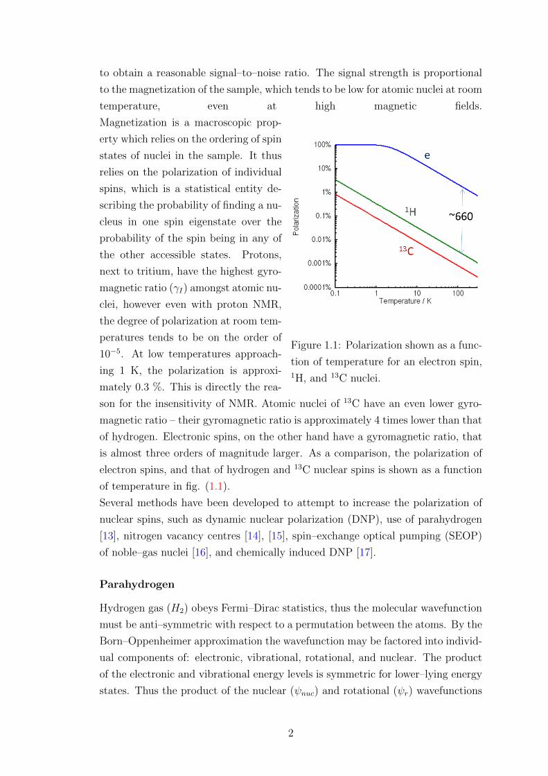
to obtain a reasonable signal–to–noise ratio. The signal strength is proportional

to the magnetization of the sample, which tends to be low for atomic nuclei at room

temperature, even at high magnetic fields.

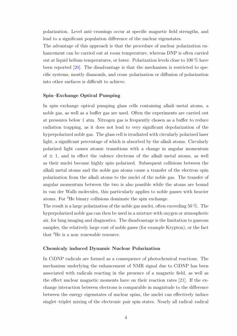
Figure 1.1: Polarization shown as a func-

tion of temperature for an electron spin,1H, and 13C nuclei.

Magnetization is a macroscopic prop-

erty which relies on the ordering of spin

states of nuclei in the sample. It thus

relies on the polarization of individual

spins, which is a statistical entity de-

scribing the probability of finding a nu-

cleus in one spin eigenstate over the

probability of the spin being in any of

the other accessible states. Protons,

next to tritium, have the highest gyro-

magnetic ratio (γI) amongst atomic nu-

clei, however even with proton NMR,

the degree of polarization at room tem-

peratures tends to be on the order of

10−5. At low temperatures approach-

ing 1 K, the polarization is approxi-

mately 0.3 %. This is directly the rea-

son for the insensitivity of NMR. Atomic nuclei of 13C have an even lower gyro-

magnetic ratio – their gyromagnetic ratio is approximately 4 times lower than that

of hydrogen. Electronic spins, on the other hand have a gyromagnetic ratio, that

is almost three orders of magnitude larger. As a comparison, the polarization of

electron spins, and that of hydrogen and 13C nuclear spins is shown as a function

of temperature in fig. (1.1).

Several methods have been developed to attempt to increase the polarization of

nuclear spins, such as dynamic nuclear polarization (DNP), use of parahydrogen

[13], nitrogen vacancy centres [14], [15], spin–exchange optical pumping (SEOP)

of noble–gas nuclei [16], and chemically induced DNP [17].

Parahydrogen

Hydrogen gas (H2) obeys Fermi–Dirac statistics, thus the molecular wavefunction

must be anti–symmetric with respect to a permutation between the atoms. By the

Born–Oppenheimer approximation the wavefunction may be factored into individ-

ual components of: electronic, vibrational, rotational, and nuclear. The product

of the electronic and vibrational energy levels is symmetric for lower–lying energy

states. Thus the product of the nuclear (ψnuc) and rotational (ψr) wavefunctions

2

must be anti–symmetric. In the presence of a magnetic field the nuclear spin

states are separated into a triplet (odd values of rotational quantum number – J;

anti–symmetric rotational wavefunction), and a singlet (even J values; symmetric

rotational wavefunction), with a population ratio of 3:1. The singlet state is re-

ferred to as parahydrogen, and transitions between the singlet and triplet states

are forbidden. At low temperatures, and in the presence of a catalyst (iron filings

or activated charcoal), it is however possible to convert the triplet state hydro-

gen nuclei to singlet states. This way the hydrogen gas becomes enriched. The

parahydrogen gas can be stored for very long periods of time, and eventually used

in a hydrogenation reaction targeting unsaturated bonds. Placing the parahydro-

gen in this kind of symmetry–breaking environment causes the protons to become

distinguishable, and thus their wavefunction changes instantaneously. This results

in the two distinct hydrogen nuclei having high polarization, which can then be

transferred to other protons in the target molecule.

The methods of sensitivity enhancement using parahydrogen in use are PASADENA

[13], where the hydrogenation reaction is carried out within a magnetic field, AL-

TADENA [13], where the hydrogenation reaction is carried out in Earth’s magnetic

field, and more recently developed SABRE [18], where signal amplification by re-

versible exchange is achieved without modification of the target molecule.

Parahydrogen induced polarization gives large signal enhancements, however the

list of molecules which these techniques can be applied to is limited, particularly

in the case of the PASADENA and ALTADENA methods – these rely on hydro-

genation of unsaturated bonds. In addition, the polarization is divided up between

protons in the target nuclei lowering their individual polarization enhancement.

Nitrogen–Vacancy centres

Nitrogen vacancy (NV) centres are defects in diamond lattice structures with a

C3v symmetry. They consist of a nitrogen–lattice vacancy electron pair oriented

along the [1,1,1] crystalline direction. These can exist in either negative (NV−) or

neutral (NV0) charge states. The two can be distinguished by their optical zero

phonon lines [19]. The NV centre exists in a triplet state (S = 1).

Laser radiation is used to excite the NV centre from its ground state (3A) to its

first excited state (3E). There processes of internal conversion and fluorescence

relaxation lead to generation of a non–Boltzmann eigenstate population, in the

triplet ground state. This is due to spin angular momentum not being conserved

in these transitions, and the degeneracy of the spin sublevels of 3A being lifted

due to the presence of a zero field splitting term. The high polarization of the

NV centre spin state can be utilised via level anti–crossing to increase the nuclear

3

polarization. Level anti–crossings occur at specific magnetic field strengths, and

lead to a significant population difference of the nuclear eigenstates.

The advantage of this approach is that the procedure of nuclear polarization en-

hancement can be carried out at room temperature, whereas DNP is often carried

out at liquid helium temperatures, or lower. Polarization levels close to 100 % have

been reported [20]. The disadvantage is that the mechanism is restricted to spe-

cific systems, mostly diamonds, and cross–polarization or diffusion of polarization

into other surfaces is difficult to achieve.

Spin–Exchange Optical Pumping

In spin–exchange optical pumping glass cells containing alkali–metal atoms, a

noble gas, as well as a buffer gas are used. Often the experiments are carried out

at pressures below 1 atm. Nitrogen gas is frequently chosen as a buffer to reduce

radiation trapping, as it does not lead to very significant depolarization of the

hyperpolarized noble gas. The glass cell is irradiated with circularly polarized laser

light, a significant percentage of which is absorbed by the alkali atoms. Circularly

polarized light causes atomic transitions with a change in angular momentum

of ± 1, and in effect the valence electrons of the alkali–metal atoms, as well

as their nuclei become highly spin–polarized. Subsequent collisions between the

alkali metal atoms and the noble gas atoms cause a transfer of the electron–spin

polarization from the alkali atoms to the nuclei of the noble gas. The transfer of

angular momentum between the two is also possible while the atoms are bound

in van der Walls molecules, this particularly applies to noble gasses with heavier

atoms. For 3He binary collisions dominate the spin exchange.

The result is a large polarization of the noble gas nuclei, often exceeding 50 %. The

hyperpolarized noble gas can then be used in a mixture with oxygen or atmospheric

air, for lung imaging and diagnostics. The disadvantage is the limitation to gaseous

samples, the relatively large cost of noble gases (for example Krypton), or the fact

that 3He is a non–renewable resource.

Chemicaly induced Dynamic Nuclear Polarization

In CiDNP radicals are formed as a consequence of photochemical reactions. The

mechanism underlying the enhancement of NMR signal due to CiDNP has been

associated with radicals reacting in the presence of a magnetic field, as well as

the effect nuclear magnetic moments have on their reaction rates [21]. If the ex-

change interaction between electrons is comparable in magnitude to the difference

between the energy eigenstates of nuclear spins, the nuclei can effectively induce

singlet–triplet mixing of the electronic pair spin states. Nearly all radical–radical

4

chemical reactions produce observable singlet–state products, the reaction rate is

thus proportional to the percentage of singlet–state radicals pairs in the system.

It has also been found to be dependent on the state of nearby nuclear spins. A

triplet pairing cannot lead to a reaction, however one of the radicals can undergo

a spin inversion – depending on the state of a nearby nuclear spin state. The

nuclear spin state has thus been compared to a catalyst [22] for the triplet to

singlet state conversion of the radical spin pair. If the nearby nuclear spin is in a

unfavourable spin state, the radicals could physically separate and react instead

with other radicals in the presence of a nucleus found in the more favourable spin

state. This leads to ordering of nuclear spin states in the product, and thus an

increased nuclear polarization.

CiDNP has use in signal enhancement of NMR, but in addition can serve as a

method for study of the reaction mechanisms of transient electron radicals in

chemistry. It is limited to use in molecules which form radicals in photochemical

reactions.

1.1 Quantum mechanical description of polar-

ization

In the presence of a static magnetic field BZ , and for ms 6= 0 the Zeeman energy

eigenstates of a spin lose their degeneracy and split according to the value of

the spin quantum number ms. The quantum number ms can take half–integer

or integer values, and for a given ms, the number of accessible Zeeman energy

eigenstates is 2×ms + 1, i.e. all possible integer–step permutations between −ms

to ms.

For ms = 12, there are two eigenstates, often denoted as |α〉, |β〉 or |↑〉,|↓〉 with

eigenvalues +12, −1

2, respectively. Throughout my work, I have focused on spin 1

2

species, hence unless otherwise stated, all relations and properties will be portrayed

for spins with ms = 12. The Zeeman energy difference, i.e. the difference in energies

between the two states for a spin-12

particle relies directly on the Larmor frequency

of a spin. The Larmor frequency of a spin is the frequency at which a spin will

precess around the magnetic field vector BZ , given as

ω = −γ ·BZ .

The constant γ is the gyromagnetic ratio of a particular nuclear spin, related to

its mass via |γ| = |e|2mg, BZ , the magnetic field strength, and g the g–factor [23].

Electrons which have a much lower mass than atomic nuclei, leading to a much

5

higher value of the gyromagnetic ratio.

The Zeeman energy eigenstates of a nuclear spin are obtained from

EZ = ω0~Iz,

where Iz for ms = 12

is a 2 × 2 Pauli σz matrix, with eigenstates +12, −1

2. Ac-

cording to Boltzmann statistics, the difference between the populations of the two

eigenstates is

∆P =e−Pα − e−Pβe−Pα + e−Pβ

=eγ~BZ2kbT − e

−γ~BZ2kbT

eγ~BZ2kbT + e

−γ~BZ2kbT

≡ tanh

(γ~BZ

2kbT

), (1.1)

where kb is the Boltzmann constant, and T the temperature of the surrounding

environment. The final product in eq. (1.1), is referred to in magnetic resonance

as the thermal polarization of that spin. Due to the relatively small gyromagnetic

ratio of nuclear spins, their Zeeman energy EZ is much smaller than the thermal

energy (kbT ). This in turn means that nuclei have low polarization. At room

temperature experiments (T = 298 K) and a field of BZ = 3.4 T, we a have

proton polarization of 1.16 × 10−5, and an electronic polarization of 7.7 × 10−3.

This is why NMR suffers from low sensitivity. Changing T to 1 K, however the

polarization values then become 3.5× 10−3 and 0.98 respectively. It is clear from

the above relation that the electron polarization rapidly approaches 100% as T→0 K.

1.2 Dynamic Nuclear Polarization

As mentioned, electron spins have a much higher gyromagnetic ratio (γS) than

nuclear spins. As a comparison to protons, the ratio of electronic γS to the nu-

clear one γI is γS/γI ≈ 658, meaning electrons will have a much higher degree of

polarization at any non–negligible magnetic field strength, and at temperatures of

T & 1. DNP is concerned with transferring the polarization from the electron to

the surrounding nuclei to create a highly polarized non–thermal state, resulting

in a large signal enhancement. The most efficient of the DNP mechanisms in the

solid state is the cross effect (CE DNP) mechanism. To date enhancements as

high as ∼400 have been achieved [24] with the use of MAS DNP, and biradical

molecules that exhibit a strong inter–electronic coupling.

In addition to a DNP–driven enhancement, rapid changes of sample temperature

may also lead to an enhancement of the signal. Using equation (1.1), it is straight–

forward to see that the ratio of polarization values for a nucleus at 1 K, to that at

room temperature results in a theoretical enhancement of 300. The total enhance-

6

ment in such case is a product of the DNP enhancement, and the enhancement

due to the temperature change

ε = εDNP × εT ,

For protons this leads to a total theoretical maximal enhancement close to 200,000.

The advantage and importance of DNP is therefore very clear.

Several applications of DNP have recently highlighted the huge potential that this

method offers for increasing the low sensitivity of MRI and spectroscopy exper-

iments [25, 26]. In particular, use of highly polarized 13C labelled molecules in

conjunction with spectroscopic MRI have led to the development of novel experi-

mental protocols for human cancer diagnostics [27, 28].

There are two types of experiments where a rapid temperature change in the sam-

ple is induced: dissolution DNP [29] and rapid temperature jump DNP [30].

In the case of dissolution DNP, a sample is cooled down to temperatures close to

1K, and irradiated with microwave radiation to build–up polarization in nuclei.

Following the build–up, the sample is dissolved and brought up to room temper-

ature with the use of hot solvents. Typically the dissolved sample would then be

either shuttled, or transferred through a magnetic tunnel to a conventional NMR

magnet. In either case a liquid–state spectrum of the sample would then be ob-

tained.

In the case of temperature jump DNP, instead of using a hot solvent, rapid heating

is applied, typically with the use of microwave radiation or optical lasers, to melt

the sample and bring it up to room temperature. A liquid state spectrum would

then be obtained. Experimental studies have been published, where with the use

of dissolution DNP enhancements of over 10,000 have been observed [29]. In the

case of temperature jump DNP, the enhancements seen have not been as large, as

previously experiments have been carried out at 90 K, with a temperature jump

to room temperature. Greater enhancements are expected in the case of a tem-

perature jump from a few Kelvin to room temperature.

1.3 DNP mechanisms

Several possible mechanisms of DNP exist. In liquid state samples, the only DNP

mechanism that is known to exist is the Overhauser effect. Predicted in theory by

Albert Overhauser in 1953 [31] to occur in metallic conductors with delocalised

electron carriers, and later in the same year verified experimentally by Carver and

Slichter [32], this is the first DNP mechanism to have been discovered. The Over-

7

hauser effect can also exist in non–metallic solid state samples which have highly

delocalised electrons; e.g. graphene samples [33]. Recent studies also suggest the

Overhauser effect can exist in solid dielectric samples undergoing periodic rotation

of MAS DNP [24]. The process of nuclear polarization build–up in static samples

is driven by cross–relaxation of an electron radical spin state, and the spin state

of a coupled nucleus, where one path of cross–relaxation has a higher rate than

the other, i.e. either the zero–quantum (ZQ) or double–quantum (DQ) transition

dominates. The cross–relaxation flips are believed to be caused by a rotational

and translational modulation of the electron–nuclear hyperfine coupling terms.

In the solid state there are additionally: the solid effect, cross effect, and ther-

mal mixing mechanisms. The solid effect mechanism is predominant in samples at

very low temperatures (few K) which have a low concentration of radical molecules.

They have narrow EPR linewidths, with very little broadening. Each radical elec-

tron is typically surrounded by several thousand nuclear spins.

The cross effect mechanism relies on electron spin pairs, thus is predominant in

samples where the radical concentration is higher and the separation between elec-

tron radicals is smaller or alternatively where bi–radical or tri–radical molecules

are used. This mechanism tends to be predominant at temperatures of a few tens

of Kelvin. In conjunction with MAS, experiments where CE–DNP is the dominant

mechanism are often carried out at liquid nitrogen temperatures. EPR spectra of

samples where CE–DNP is active are typically broad and inhomogeneous, and the

electron radicals exist in a large variety of magnetic environments.

Thermal mixing (TM) is a many–body process of a strongly coupled electronic

network interacting with atomic nuclei. This mechanism is the dominant DNP

pathway when the homogeneous (and typically the inhomogeneous too) broad-

ening is significantly greater than the nuclear Larmor frequency ωI < η, ζ. Due

to the exponential growth of the Liouville space with respect to an increasing

number of simulated spins, it is difficult to describe thermal mixing systems using

quantum–mechanical approaches. Such attempts are limited – one example of

such work is by Hovav et al. [34]. Thermodynamic approaches are usually used

for a description of TM. In these approaches the system is usually described as

consisting of three spin reservoirs [35], and the principle of spin temperature is

used in describing nuclear polarization enhancement. Often more than one DNP

mechanism would be active in a sample, and in certain circumstances DNP mech-

anisms are incorrectly categorised as thermal mixing, when in fact a mixture of

SE and CE–DNP takes place [36].

8

1.4 Current work

My PhD project was focused on the theory and spin dynamics of DNP. Although

DNP has already been successfully used in a variety of applications, outlined

above, the theory underlying the mechanisms is not yet entirely understood. A

lot of insight has already been provided by small spin system simulations in pre-

vious work by ourselves and others [37, 38, 36, 39], but what is missing is insight

into large spin system simulations. This in particular applies to understanding the

transport of polarization into the bulk of the sample or when conducting studies

into the optimisation of the DNP mechanisms to improve steady–state polariza-

tion and reduce the build–up times. More insight and a better understanding of

the physics underlying DNP will lead to improvement of signal enhancement in

applications, where DNP is already proven as a useful tool.

In addition, we believe that the systems exhibiting DNP are of interest to a much

wider community conducting research into dissipative quantum systems. SE–DNP

can be described as a central spin model, with the electron spin in the centre, driv-

ing nuclear spins out of thermal equilibrium. In CE–DNP, we have a case where

a three–spin mechanism dominates over a two–spin mechanism, and the two elec-

trons act as one entity, which is much more efficient than two individual electron

sources exhibiting SE–DNP would be.

The aim of my project was therefore to develop new methodology for modelling

and simulating the DNP mechanisms in order to gain an improved understanding

of the underlying physics, and to seek ways to potentially improve the detected sig-

nal enhancements. We sought an approach which would allow simulations of spin

systems much larger than was at the time possible, to gain more understanding of

DNP. In the case of SE–DNP, one electron is typically surrounded by thousands

of nuclear spins – our goal was to make such simulations possible, and in effect

attempt to make the simulations more realistic.

Using mathematical techniques of adiabatic elimination, novel tools were devel-

oped for SE–DNP and CE–DNP allowing simulations with numbers of spins three

orders of magnitude greater than was previously possible. This was carried out

by projecting the dynamics of each mechanism onto the population subspace of

the density operator. With this procedure, effective rate equations are extracted

from the full dynamics. These rates resemble classical state–dependent dynamics

and in such form provide new, clearer insight into these mechanisms of DNP.

Simulations were then implemented for 1–D spin chain systems in order to test

an existing hypothesis [38] regarding transport of polarization in SE–DNP. It was

shown that contrary to the previous model, transport of polarization into the bulk

9

is governed by spin–diffusion. Polarization transport pathways were fitted to a

solution to the diffusion equation, more importantly however, it was discovered

that a reflective boundary solution fits the simulated data much more closely. This

highlighted the importance of large spin system simulations: small spin systems

suffer severely from finite, reflective boundaries.

A large spin simulation involving 1331 spins was implemented to show the capa-

bility of our approach. The result was compared to a simulation where nuclear

dipolar interactions were set to 0, to show spin diffusion effects in a 3–D lattice.

A study into radical efficiency was then carried out, where a total of 26 nuclei

out of 124 were subsequently removed from the system – a study as such is only

possible with our formalism, as full master equation approaches are limited to a

few spins. The study shows that removal of core nuclei can increase the polariza-

tion of the bulk, and thus an optimal separation between the electron and nearest

surrounding nuclei exists, and the formalism has radical study and optimisation

capability. A similar formalism for heteronuclear simulations was derived, and in

addition simulations using a linear rate approach were implemented for a system,

of 9260 13C nuclei.

For CE–DNP, the effective rate treatment showed that the SE–DNP mechanism is

still present in cases of electron radical pairs. The mechanism of polarization trans-

port was confirmed to again be spin–diffusion. A comprehensive error analysis

showed the suitability of the formalism for studies of bi–radicals or mono–radicals

in close proximity. It was discovered that the rate corresponding to the three–spin

process of CE–DNP corresponded well to a region of shortest polarization build–

up, and greatest steady–state nuclear polarization. The form of the effective rates

shows a dependence of rate magnitude on relaxation parameters, microwave field

amplitude, and electronic dipolar coupling strength. Varying those terms leads

to the possibility of optimisation and design of bi–radicals, which our formalism

holds. Large spin system simulations were then carried out with more optimal

parameters.

1.5 Thesis structure

The thesis is divided into four main chapters, not including the introduction.

Chapter 2 is a theory chapter. The theory of open quantum systems is first

described, including the Kraus operator formalism and the Lindblad master equa-

tion. The theory of SE–DNP as well as CE–DNP are discussed in depth. Following

this, the general principle of adiabatic elimination and separation of subspaces is

described. In the last section the kinetic Monte Carlo algorithms, and their use

are described.

10

Chapter three is focused entirely on SE–DNP. Firstly, the explicit derivation

of the effective dynamics using adiabatic elimination is shown and discussed, in-

cluding a qualitative description of the effective dynamics. In the next section

a comprehensive error analysis is shown. This is followed by an analysis of the

polarization transport in spin ensembles, and simulations of large spin systems.

The scaling of Monte Carlo error and the simulation duration, with respect to an

increasing number of spins are quantified and discussed. In section 6, we show

how the effective dynamics can be extended to hetero–nuclear systems that are

close in frequency. The final part of this chapter shows our linear–rate approach

to SE–DNP, suitable for simulating systems of nuclei with lower gyromagnetic

ratios (13C is a perfect ’candidate’). This approach avoids the use of Monte Carlo

algorithms, and allows simulations of spin systems consisting of 10s of thousands

of spins in a manner of minutes.

In chapter four the effective formalism from chapter three is used to study the

effect of removing core nuclei from a spin system. A tightly bound lattice of 12413C nuclei and one central electron is used. Core nuclei are subsequently removed

from the system, and the effect this has on the polarization of the ensemble is

studied. We show that these spin systems intricately depend on the parameter

choice, and an optimal separation between the central electron and nearest nuclei

can be found, leading to an improved polarization transfer to the ensemble. We

illustrate how this works using simulated DNP frequency spectra, and discuss the

potential this holds for radical study and design.

Our work on cross effect DNP is described in chapter five. First the deriva-

tion of the effective dynamics is shown. The conditions for which the projection

is valid are shown, and the effective rates leading to polarization build–up are

individually described. The effective rates alone already provide a lot of insight

into the mechanism of CE–DNP. A comprehensive error analysis follows, and we

show the parameter region for which our formalism is valid, as well as showing

how regions of excessive error can be predicted. The formalism is suitable for

simulating systems of bi-radicals or mono-radicals in a relatively close proximity,

up to approximately 40 A. We then show that polarization transport in CE–DNP

is also governed by spin diffusion. In the last section of chapter five, we show

the dependence of nuclear polarization on the system parameters, especially on

the electronic dipolar coupling strength, and their decoherence rate. We show

the potential our formalism holds in bi-radical study, design and optimisation,

as the effective rate for the three–spin process is seen to correspond to areas of

11

shortest polarization build–up and largest steady–state polarization levels in the

ensemble. We show one example simulation as a comparison to SE–DNP where a

good parameter choice leads to polarization build-up in CE–DNP being orders of

magnitude faster.

In chapter six we present a summary and conclusion of our work to date, as

well as an outlook into future research our group intends to conduct.

12

Chapter 2

Theory

This chapter summarises the theory behind dynamic nuclear polarization, start-

ing from a quantum-mechanical description of the problem. Relaxation plays a

very important role in DNP, and coherent evolution alone does not explain the

phenomenon of polarization transfer. A closed system quantum-mechanical de-

scription of the problem is not suitable and one has to turn to the open quantum

system approach, where relaxation of the system is described by a semi-classical

phenomenological interaction with an effective environment. The theory of open

quantum systems including the Kraus operator formalism and the Lindbladian

approach are described in this chapter.

2.1 Open quantum systems - relaxation theory

An important starting point of the description of quantum mechanics of a many-

body spin system is the density operator formalism.

2.1.1 The density operator formalism

For small spin systems (e.g. particle in an infinite energy well, or free electron

approaching potential barrier) a suitable wavefunction is chosen, the squared am-

plitude of which corresponds to a probability of locating that particle at a par-

ticular point in space (and possibly time). The system Hamiltonian describes the

interactions of the particle. For states stationary in time the time-independent

Schrodinger is solved

H |Ψ〉 = E |Ψ〉 . (2.1)

13

Otherwise, if the wavefunction evolves under the action of a closed-system Hamil-

tonian, then the time-dependent variant of eq. (2.1) is used

i~∂

∂t|Ψ〉 = H |Ψ〉 . (2.2)

However, for systems of 2 or more interacting particles, equation (2.2) becomes

increasingly difficult to solve. The particles are often coupled with coherences

existing between their states, and the dynamics of each particle become difficult

to separate. The usual method of separating variables cannot be applied. One

should instead use the density operator formalism. If the system can be described

by a set of ortho-normal (orthogonal and normalised) quantum states |Ψ〉 = c1ψ1+

c2ψ2 + ...+ckψk, with associated normalisation coefficients c1, c2, ..., ck, the density

operator is defined as

ρ = |Ψ〉 〈Ψ| ≡∑k

pk |ψk〉 〈ψk| , (2.3)

where pk = |ck|2 are probabilities of the system existing in a particular state.

The density operator has the following properties:

1. it is a Hermitian operator ρ† = ρ. For a complete set of basis states, it can

be represented as a matrix – the dagger denotes a Hermitian conjugate

2. due to the Hermitian property ρ has real eigenvalues, and if Ψ is ortho-

normal these eigenvalues are pk, where 0 ≤ pk ≤ 1

3. the trace Tr (ρ) of the density operator equals 1, if the underlying quantum

states are properly normalised

4. the expectation value of any operator can be calculated if ρ is known:⟨X⟩

=

Tr(Xρ)

.

In the case that one of the pk = 1, and the others are 0, the density operator

represents a pure state. This implies there is 100% probability of finding the

system in the corresponding state |ψk〉 〈ψk|. Otherwise the system is in a mixed

state. The measure of how mixed the states of a density operator are is Tr(ρ2).

A trace value of 1 implies a pure state, while a trace value of <1 denotes a mixed

state. Due to a small degree of polarization in NMR, as shown in eq. (1.1), nuclear

states are always mixed. At very low temperatures and moderate-high magnetic

fields, electronic spin states are approximately pure states.

14

To find the time evolution of the density operator, eq. (2.2) is used.

∂

∂t|Ψ〉 = − i

~H |Ψ〉 conjugating both sides gives

∂

∂t〈Ψ| = i

~〈Ψ| H

hence

∂

∂tρ ≡ ∂

∂t(|Ψ〉 〈Ψ|) =

∂ |Ψ〉∂t〈Ψ|+ |Ψ〉 ∂ 〈Ψ|

∂t= − i

~H |Ψ〉 〈Ψ|+ i

~|Ψ〉 〈Ψ| H

∂

∂tρ = − i

~

[H, ρ

]. (2.4)

Equation (2.4) is called the Liouville von Neumann (LvN) equation, and it de-

scribes the time-evolution of a closed quantum system with density operator ρ.

As a final point, it is worth mentioning that the thermal equilibrium density op-

erator is well approximated by

ρth =z

Tr (z), where z = exp

(− ~HkbT

), (2.5)

for a thermal equilibrium Hamiltonian containing no time-dependent interactions,

i.e. the system is not driven.

This form of the LvN equation describes unitary evolution, of a closed quantum

system. A dissipative part can be added to accommodate for relaxation in an

open quantum system.

For a two-spin system, for any given state of spin 1, spin 2 can exist in any of

its accessible states. The states of each spin are independent of each other, hence

when computing the total density operator for the two spins, a direct product ⊗is used

ρA = ρ1 ⊗ ρ2.

For an ensemble of spins, each having independent states, the ensemble density

operator consists of a product of the individual spin density operators

ρA = ρ1 ⊗ ρ2 ⊗ ρ3 ⊗ · · · ⊗ ρn.

For spin 12

particles the dimension of the density operator of a single spin is 21,

for a two-spin system, this dimension becomes 22. In general the system density

operator scales as 2n for n spins, and has (2n)2 = 4n elements.

15

2.1.2 Quantum operation

The theory in this section is described in detail by Preskill [40] and Fisher [41].

As mentioned previously, the systems we deal with in DNP are not isolated sys-

tems. These are subject to dissipation due to their coupling to the environment

(often referred to as the lattice in NMR), and as such an open quantum system

approach is necessary.

The system of interest (A) and coupled environment (E) behave together as an

entangled bipartite system. The entire system density operator is of the form of

ρ = ρA⊗ ρE, where ⊗ is again a direct product signifying that for a given state of

the system - A , the environment may exist in any one of its possible states and

vice versa. A pure state of the bipartite system may behave like a mixed state

when A is observed alone [40], and an orthogonal measurement of the bipartite

system may be a non-orthogonal positive operator-valued measure on A alone. If

a state of the bipartite system undergoes unitary evolution, the problem is at-

tempting to describe the evolution of A alone.

Supposing the initial density matrix of the bipartite system is a tensor product

state of the form

ρA ⊗ |0〉E E〈0|,

the system has density operator ρA, and the environment is in a pure state |0〉E.

The whole system evolves under the action of a unitary time evolution operator

UAE :

UAE (ρA ⊗ |0〉E E〈0|) U†AE,

a partial trace is performed over the Hilbert space of the environment HE to find

the density matrix of the system A

ρ′A = TrE

(UAE (ρA ⊗ |0〉EE〈0|) U

†AE

)=∑µ

E〈µ|UAE |0〉E ρA E〈0|U†AE |µ〉E ,

where 〈µ|E is an orthonormal basis for HE and in such case E〈µ|UAE |0〉E is an

operator acting on HA.

If the unitary operator acting in the subspace H of density operator ρA is denoted

as

Mµ = E〈µ|UAE |0〉E ,

the evolution in this subspace is expressed as

ρ′A ≡ X (ρA) =∑µ

MµρAM†µ. (2.6)

16

Because the evolution of ρA ⊗ |0〉E E〈0| is unitary under UAE, the operators M in

eq. (2.6) satisfy the property∑µ

M †µMµ =

∑µ

E〈0|U†AE |µ〉E E〈µ|UAE |0〉E

= E〈0|U†AEUAE |0〉E = 1A. (2.7)

Throughout the thesis bold notation is used for superoperators. In equation

(2.6) X is a linear map, taking linear operators to linear operators. This map is

called a superoperator or a quantum operation. The representation of X is called

an operator sum representation or Kraus representation of a superoperator, where

Mµ are the Kraus operators. Unitary evolution is invertible; there exists an inverse

that can reverse the evolution of the system, forming an analogy to time-reversal.

Unitary evolution forms a group. Superoperators describing non-unitary evolu-

tion define a dynamical semigroup. Decoherence, a dissipative process due to the

interaction with the environment is an irreversible process that defines an arrow

of time in quantum dynamics. As such, decoherence leads to an irreversible loss

of information any real system is subject to – truly closed quantum systems do

not exist in reality.

Map X takes an initial density operator to a final density operator

X : ρ→ ρ′.

There are a set of properties this map has to satisfy to make it physical:

1. X must preserve hermiticity; ρ′ will be hermitian if ρ is

2. X should be linear

3. X must be trace preserving, and therefore preserve the normalisation of the

density operator; if Tr(ρ) = 1, Tr(ρ′) = 1

4. X is completely positive.

The complete positivity is a requirement that if any possible environment is chosen,

coupled to the system, resulting in a joint density matrix ρ = ρA ⊗ ρE, the result

of a composite operation (map ξ)

ξρ =(X⊗ 1

)(ρA ⊗ ρE)

is another positive operator; X is completely positive acting on the subspace of

ρA if X ⊗ 1 is positive for any coupled environment. This is a consequence of

17

the fact that a quantum system is not completely isolated, and one can never

be certain that when studying the evolution of the system A, it isn’t coupled to

some environment. If the system evolved but the environment does not, complete

positivity ensures the density operator will evolve to another density operator.

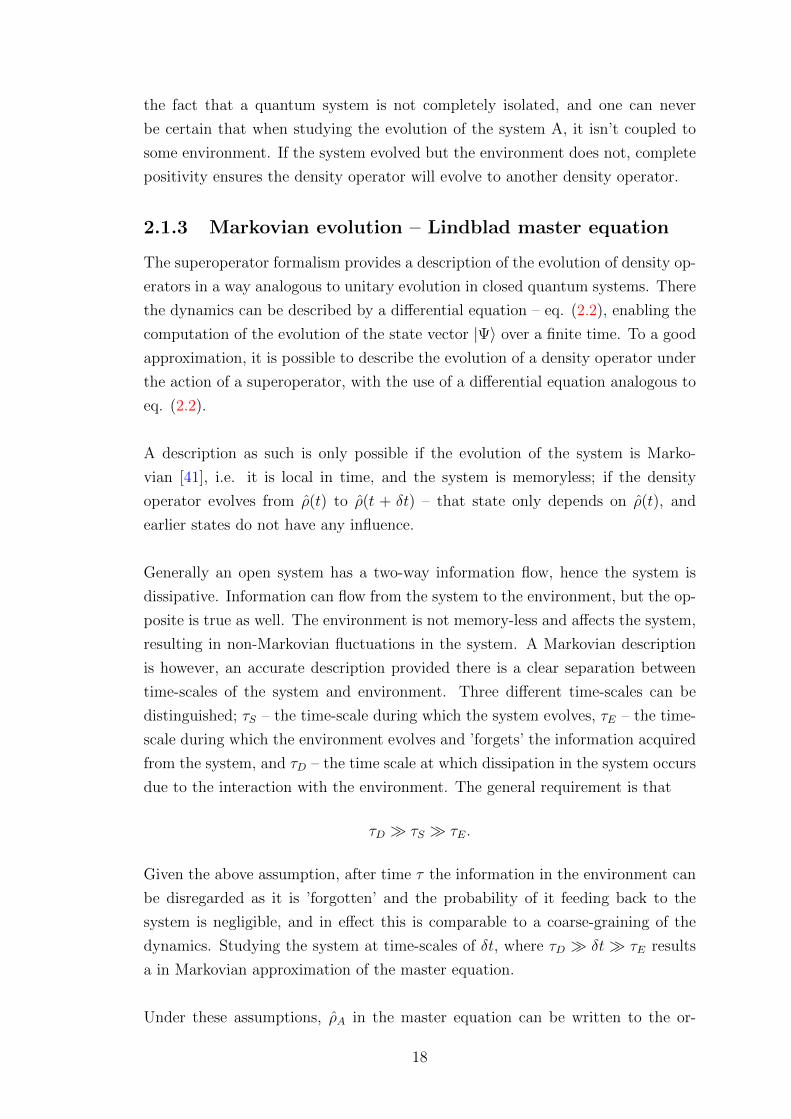
2.1.3 Markovian evolution – Lindblad master equation

The superoperator formalism provides a description of the evolution of density op-

erators in a way analogous to unitary evolution in closed quantum systems. There

the dynamics can be described by a differential equation – eq. (2.2), enabling the

computation of the evolution of the state vector |Ψ〉 over a finite time. To a good

approximation, it is possible to describe the evolution of a density operator under

the action of a superoperator, with the use of a differential equation analogous to

eq. (2.2).

A description as such is only possible if the evolution of the system is Marko-

vian [41], i.e. it is local in time, and the system is memoryless; if the density

operator evolves from ρ(t) to ρ(t + δt) – that state only depends on ρ(t), and

earlier states do not have any influence.

Generally an open system has a two-way information flow, hence the system is

dissipative. Information can flow from the system to the environment, but the op-

posite is true as well. The environment is not memory-less and affects the system,

resulting in non-Markovian fluctuations in the system. A Markovian description

is however, an accurate description provided there is a clear separation between

time-scales of the system and environment. Three different time-scales can be

distinguished; τS – the time-scale during which the system evolves, τE – the time-

scale during which the environment evolves and ’forgets’ the information acquired

from the system, and τD – the time scale at which dissipation in the system occurs

due to the interaction with the environment. The general requirement is that

τD � τS � τE.

Given the above assumption, after time τ the information in the environment can

be disregarded as it is ’forgotten’ and the probability of it feeding back to the

system is negligible, and in effect this is comparable to a coarse-graining of the

dynamics. Studying the system at time-scales of δt, where τD � δt � τE results

a in Markovian approximation of the master equation.

Under these assumptions, ρA in the master equation can be written to the or-

18

der of δt, ensuring linearity

ρA (δt) = XρA (0) ≡∑µ

MµρA (0) M †µ = ρA (0) +O (δt) .

Dictated by the order with respect to time, and the form of X, the Kraus operators

must be of the form

M0 = 1S +

(K − i

~H

)δt (2.8)

Mk =√δtLk (for k ≥ 1) , (2.9)

where H is the system Hamiltonian, operators Lk are later defined as Lindblad

jump operators, and K is an arbitrary hermitian operator, the need for which is

shown later. The condition in eq. (2.7) requires∑µ

M †µMµ = 1A

which implies

1A = 1A +

(2K +

∑k

L†kLk

)δt+ 0(δt)2,

thus

K = −1

2

∑k

L†kLk

is a normalisation term, required in evolution time-steps where no quantum jumps

occur. Hence

ρA(δt) =

[1S +

(K − i

~H

)δt

]ρA(0)

[1S +

(K +

i

~H

)δt

]+∑k

LkρA(0)L†k

= ρA(0) + ρA(0)

[K +

i

~H

]δt+

[K − i

~H

]ρA(0)δt+

∑k

LkρA(0)L†kδt

= ρA(0)− i

~

[H, ρA(0)

]δt+

∑k

[LkρA(0)L†k −

1

2

{ρA(0), L†kLk

}]δt.

Following the standard definition of derivatives, where

˙ρA (0) = limδt→0

ρA(0 + δt)− ρA(0)

δt

19

we have the form of the master equation

limδt→0

ρA(0 + δt)− ρA(0)

δt≡ ˙ρA(0)

= − i~

[H, ρA(0)

]+∑k

[LkρA(0)L†k −

1

2

{ρA(0), L†kLk

}]

and have thus derived the Lindblad master equation for the density operator of

system (A) coupled to the environment (E)

dρ

dt= Lρ ≡ −i

[H, ρ

]+∑k

D[Lk

]ρ. (2.10)

The Hamiltonian is in the frequency domain (divided by ~). The Lindblad dissi-

pator superoperator is of the form

D[Lk

]ρ = LkρL

†k −

1

2

{ρ, L†kLk

}. (2.11)

The dissipative part – eq. (2.11) – is responsible for relaxation in the system.

Different relaxation pathways are modelled with so-called Lindblad jump op-

erators, Lk. These operators cause instantaneous jumps between eigenstates of

the system. The form of these operators is described further in this chapter in

section 2.1.5. The square bracket represents a commutator relation, and corre-

sponds to the coherent part of the master equation. The curly bracket represents

an anti-commutator relation. The master equation as a whole describes a non-

unitary evolution of the density operator in the Markovian Limit. In the case of no

dissipative pathways, the standard LvN equation (2.4) is recovered, and unitary

evolution would be seen. The Hamiltonian H, however, is not necessarily identical

to the Hamiltonian of the closed system – in some cases important corrections will

be seen [41] in the system Hamiltonian due to the interaction with the environ-

ment (E). The environment our system is coupled to evolves on a time-scale that

is much shorter than the system-evolution time-scale; the information flow from

the system to the environment is by assumption non-reversible on the time-scale

over which the system evolves.

2.1.4 Lindblad propagator

The form of eq. (2.10) makes analytical integration difficult, particularly for sys-

tems consisting of more than 1 spin. An ordinary differential equation solver may

be employed to find numerical solutions.

It is however possible to re-write the form of eq. (2.10) to act in Liouville space,

i.e. operator space, in which case the result is a Lindblad superoperator acting on

20

the density operator from the left. A simple method for conversion of the form of

the master equation has been presented by Tim Havel [42]. A superoperator form

of eq. (2.10) is obtained by again starting from the Kraus formalism. It is proven

in the text that eq. (2.6) is equivalent to

X(ρ) =∑µ

(M∗

µ ⊗ Mµ

)ρA,

where the asterisk denotes a complex conjugate (M †)T ≡ M∗, where T denotes a

transpose.

Plugging in the Kraus operators of the form shown in eqs. (2.8, 2.9);∑µ

(M∗

µ ⊗ Mµ

)= δt

(1 +

(K − iH

))∗⊗(

1 + K − iH)δt+ δt

∑k

L∗k ⊗ Lk.

Since (A+B)∗ ≡ A∗ +B∗, and (−iA)∗ ≡ iA∗, this becomes

∑µ

(M∗

µ ⊗ Mµ

)= δt

(1⊗ K − i1⊗ H + iH∗ ⊗ 1 + K∗ ⊗ 1 +

∑k

L∗k ⊗ Lk

),

which in a manner similar to deriving eq. (2.10) results in

L = i(H∗ ⊗ 1− 1⊗ H

)+∑k

(L∗k ⊗ Lk −

1

21⊗ L†kLk −

1

2

(L†kLk

)∗⊗ 1

).

(2.12)

Here, the identity operators 1 have the same dimension as the Hamiltonian and

Lindblad jump operators. The superoperator L acts on the density operator from

the left, it is therefore straightforward to solve the differential equation for the

evolution of ρ in time to give the form of the time-propagator

dρ

dt= Lρ =⇒ ρ(t) = eLtρ(0). (2.13)

Previously, the dimension of the Lindbladian eq. (2.10) would be equivalent to

the density operator dimension i.e. 2n, for n spins. Rewriting the Lindbladian

in the form of eq. (2.12) makes the Liouville space dimension it acts on scale as

4n. The density operator this form of master equation acts on is column-stacked,

resulting in a size of 4n × 1, in which case eq. (2.13) is strictly written as

col ρ(t) = eLt col ρ(0).

Despite the increased space dimension, this form of the master equation provides

an advantage computationally.

21

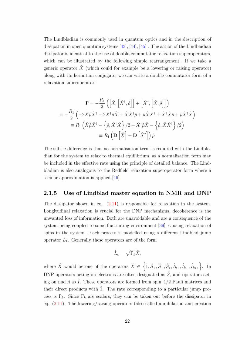
The Lindbladian is commonly used in quantum optics and in the description of

dissipation in open quantum systems [43], [44], [45] . The action of the Lindbladian

dissipator is identical to the use of double-commutator relaxation superoperators,

which can be illustrated by the following simple rearrangement. If we take a

generic operator X (which could for example be a lowering or raising operator)

along with its hermitian conjugate, we can write a double-commutator form of a

relaxation superoperator:

Γ = −R1

2

([X,[X†, ρ

]]+[X†,

[X, ρ

]])≡ −R1

2

(−2XρX† − 2X†ρX + XX†ρ+ ρXX† + X†Xρ+ ρX†X

)≡ R1

(XρX† −

{ρ, X†X

}/2 + X†ρX −

{ρ, XX†

}/2)

≡ R1

(D[X]

+ D[X†])ρ.

The subtle difference is that no normalisation term is required with the Lindbla-

dian for the system to relax to thermal equilibrium, as a normalisation term may

be included in the effective rate using the principle of detailed balance. The Lind-

bladian is also analogous to the Redfield relaxation superoperator form where a

secular approximation is applied [46].

2.1.5 Use of Lindblad master equation in NMR and DNP

The dissipator shown in eq. (2.11) is responsible for relaxation in the system.

Longitudinal relaxation is crucial for the DNP mechanisms, decoherence is the

unwanted loss of information. Both are unavoidable and are a consequence of the

system being coupled to some fluctuating environment [39], causing relaxation of

spins in the system. Each process is modelled using a different Lindblad jump

operator Lk. Generally these operators are of the form

Lk =√

ΓkX,

where X would be one of the operators X ∈{

1, S+, S−, Sz, Ik+, Ik−, Ikz,}

. In

DNP operators acting on electrons are often designated as S, and operators act-

ing on nuclei as I. These operators are formed from spin–1/2 Pauli matrices and

their direct products with 1. The rate corresponding to a particular jump pro-

cess is Γk. Since Γk are scalars, they can be taken out before the dissipator in

eq. (2.11). The lowering/raising operators (also called annihilation and creation

22

Figure 2.1: Illustration of the processes of londitudinal (T1) relaxation – left partof figure, and transverse (T2) relaxation – right part of figure, modelled usingLindblad jump operators. Operators consisting of σ± cause jumps between theeigenstates (energy levels) of the system, and are weighted by the thermal po-larization coefficient, eq. (1.1), so that in the absence of coherent evolution thesystem will relax back to its thermal equilibrium state (LHS figure). Operatorsconsisting of σz, cause decoherence (RHS figure) of the spin state, i.e. causingspins to go out of phase with respect to one another.

operators) are of the form S± = Sx ± iSy and Ik± = Ikx ± iIky for electrons and

nuclei respectively.

The operators S±, Ik± are responsible for transitions between eigenstates of the

system and introduce longitudinal relaxation in the system. The operators Sz, Ikz

are mainly responsible for decay of coherences in the system. In fig. 2.1, left, a

schematic representation of transitions leading to dissipation due to T1 processes

is shown. Operators containing σ+ will cause transitions from the eigenstate E1

to the state E2, with a rate Γ+ = R1

2(1 + pth) The opposite is true for operator

σ−, where the transition rate is Γ− = R1

2(1− pth). The two rates are weighted by

the thermal equilibrium polarization of a spin, to ensure that spin relaxes back

to thermal equilibrium without any driving of the system. In fig. 2.1, right, dis-

sipation due to T2 processes is shown in a similar manner. Dissipation due to T2

processes leads to the spins coming out of phase with respect to one another. The

rate associated with this process is Γz = 2R2. The dissipative processes due to T1

and T2 are both incoherent and irreversible.

Using this dissipator form it is straight-forward to introduce more complicated re-

laxation pathways for the system (e.g. spin cross-relaxation). In [39] we discussed

the differences in simulations seen between using a Lindblad form dissipator de-

fined in the Zeeman basis, and the relaxation superoperator form used by Hovav

et al. [37] in the eigenbasis of the stationary Hamiltonian. Furthermore, we de-

scribe in [39] the possibility of addition of other dissipation parts to the relaxation

23

superoperator.

2.1.6 Link between quantum and classical dynamics

The expectation value for an arbitrary operator X is given as⟨X⟩

= Tr(ρX)≡ Tr

(Xρ).

Using the Lindblad master equation – eq. (2.10), and multiplying it from the left

by a spin operator X, if the trace of both sides is taken; the time-evolution of the

expectation value of the operator X can be found:⟨dX

dt

⟩= −i T r

[X[H, ρ

]+ X

∑k

(LkρL

†k −

1

2

{ρ, L†kLk

})].

The cyclic properties of the trace operation can then be used to give a slightly

altered form of eq. (2.10), used for the expectation value of an operator X

⟨˙X⟩

=

⟨i[H, X

]+∑k

(L†kXLk −

1

2

{X, L†kLk

})⟩. (2.14)

Using eq. (2.14) for a single isolated electronic spin, the expectation values were

obtained for each operator in the basis

X ∈{

1, S+, S−, Sz

},

with Hamiltonian H = ∆Sz + ω1

2(S+ + S−), and Lindblad jump operators L+ =

R1(1− pth)/2, L− = R1(1 + pth)/2, Lz = 2R2. The result is given as:⟨˙S+

⟩= −iω1

⟨Sz

⟩+ {i∆−R2}

⟨S+

⟩⟨

˙S−

⟩= iω1

⟨Sz

⟩+ {−i∆−R2}

⟨S−

⟩⟨

˙Sz

⟩=

i

2ω1

⟨S−

⟩− i

2ω1

⟨S+

⟩−R1

⟨Sz

⟩+

1

2pthR1

⟨1⟩,

and the time-evolution of the expectation value of identity is 0. The operator

expectation value time evolution equations can be represented in matrix form⟨S+

⟩⟨S−

⟩⟨Sz

⟩ =

i∆−R2 0 −iωA0 −i∆−R2 iωA−iωA

2iωA

2-R1

〈S+〉〈S−〉〈Sz〉

+

0

012pthR1

24

which has the equation form of

〈s〉 = M 〈s〉+ b. (2.15)

Setting the left hand side of eq. (2.15) to 0, the steady-state solutions for the

operator values are obtained:

〈s〉ss = −M−1 (b)

⟨S+

⟩ss⟨

S−

⟩ss⟨

Sz

⟩ss

=12pthR1

R1 (∆2 +R22) +R2ω2

1

−iω1 (i∆ +R2)

−iω1 (i∆−R2)

(∆2 +R22)

,

from which the classical steady-state Bloch equations are recovered

⟨Sx

⟩ss

=ω1∆ (T2)2

1 + (∆T2)2 + ω21T1T2

· pth

2⟨Sy

⟩ss

=−ω1T2

1 + (∆T2)2 + ω21T1T2

· pth

2⟨Sz

⟩ss

=1 + (∆T2)2

1 + (∆T2)2 + ω21T1T2

· pth

2.

In some circumstances, coupling to the environment causes an object to behave

’classically’ even though the intrinsic dynamics of the system are quantum. This

has led some to speculate [41] that the open quantum system approach provides

a link between quantum mechanics and the macroscopical classical limit.

2.2 Theory of solid effect DNP

In this section, the theory of SE-DNP is described on a microscopic scale. This

mechanism is most pronounced at low temperatures, when low radical concen-

trations are used. In such case, the dipolar coupling between electron radicals is

negligible and a central electron spin model [47] is suitable for modelling SE-DNP

dynamics. A basic description entails an electron spin surrounded by atomic nu-

clei. Polarization is transferred to nuclei surrounding the electron, these nuclei in

turn transfer their polarization to the bulk via nuclear dipole-dipole interaction.

25

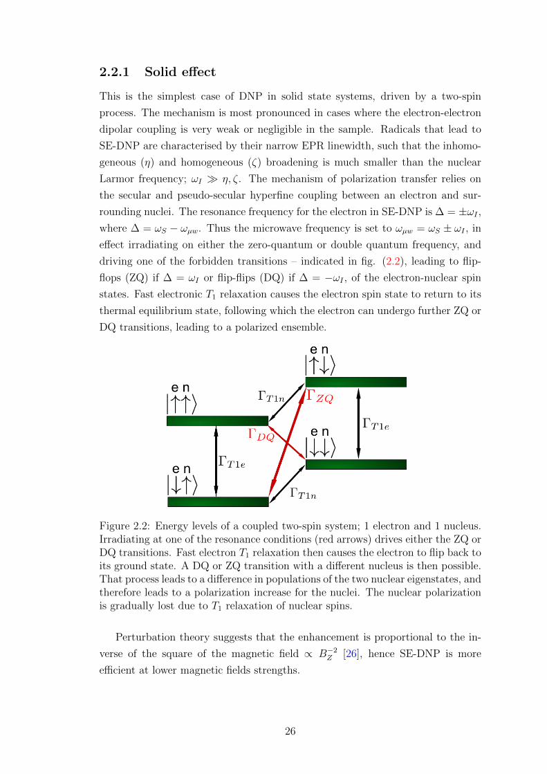
2.2.1 Solid effect

This is the simplest case of DNP in solid state systems, driven by a two-spin

process. The mechanism is most pronounced in cases where the electron-electron

dipolar coupling is very weak or negligible in the sample. Radicals that lead to

SE-DNP are characterised by their narrow EPR linewidth, such that the inhomo-

geneous (η) and homogeneous (ζ) broadening is much smaller than the nuclear

Larmor frequency; ωI � η, ζ. The mechanism of polarization transfer relies on

the secular and pseudo-secular hyperfine coupling between an electron and sur-

rounding nuclei. The resonance frequency for the electron in SE-DNP is ∆ = ±ωI ,where ∆ = ωS − ωµw. Thus the microwave frequency is set to ωµw = ωS ± ωI , in

effect irradiating on either the zero-quantum or double quantum frequency, and

driving one of the forbidden transitions – indicated in fig. (2.2), leading to flip-

flops (ZQ) if ∆ = ωI or flip-flips (DQ) if ∆ = −ωI , of the electron-nuclear spin

states. Fast electronic T1 relaxation causes the electron spin state to return to its

thermal equilibrium state, following which the electron can undergo further ZQ or

DQ transitions, leading to a polarized ensemble.

Figure 2.2: Energy levels of a coupled two-spin system; 1 electron and 1 nucleus.Irradiating at one of the resonance conditions (red arrows) drives either the ZQ orDQ transitions. Fast electron T1 relaxation then causes the electron to flip back toits ground state. A DQ or ZQ transition with a different nucleus is then possible.That process leads to a difference in populations of the two nuclear eigenstates, andtherefore leads to a polarization increase for the nuclei. The nuclear polarizationis gradually lost due to T1 relaxation of nuclear spins.

Perturbation theory suggests that the enhancement is proportional to the in-

verse of the square of the magnetic field ∝ B−2Z [26], hence SE-DNP is more

efficient at lower magnetic fields strengths.

26

2.2.2 Hamiltonian

The Hamiltonian for the central spin model is of the form

H = HZ + HIS + HII + Hmw. (2.16)

Due to the presence of a magnetic field, each spin has its Larmor frequency with

which it precesses around the vector of the magnetic field BZ , and each spin

therefore has a Zeeman energy. The Zeeman Hamiltonian has the form

HZ = ωSSz + ωI∑k

Ikz.

The Larmor frequency of electron spins (ωS) is orders of magnitude greater than

that of atomic nuclei (ωI). In addition to the Zeeman terms, there exists a hy-

perfine coupling between the nuclei and the electron. It consists of two parts; the

Fermi contact interaction and the dipolar coupling interaction. The Fermi contact

interaction is scaled by the squared absolute value of the electronic wavefunction,

calculated at the position of the nucleus. This term tends to only be relevant

for nuclei that are very close to the electron, but is generally not important for

the DNP mechanisms; the contribution of the Fermi contact interaction is a shift

in frequency of nuclei close to the electron. The dipolar part of the hyperfine

interaction is in the form of a tensor interaction, and has the general form

HIS =∑k

S ·↔A · Ik, (2.17)

where the full form of S ·↔A · Ik is

S ·↔A · I = a1Sz Iz + a2Sz I+ + a3Sz I− + a4S+Iz + a5S+I+

+ a6S+I− + a7S−Iz + a8S−I+ + a9S−I−.

The coupling strength coefficients ai depend on the separations and relative po-

sitions of the electron and surrounding nuclei. Generally the coupling strength

scales proportionally to the cubic inverse of the separation between the spins.

The Hamiltonian part HII describes interactions between the nuclei. In moderate

to high magnetic fields only the secular part of the dipolar Hamiltonian needs to

be considered, so the Hamiltonian takes the form

HII =∑kk′

dkk′

(2Ikz Ik′z −

1

2Ik+Ik′− −

1

2Ik−Ik′+

),

27

where the coupling parameter dkk′ has the form

dkk′ = −µ0

4π

γ(I)k γ

(I)k′ ~

2r3kk′

(3 cos(Θkk′)− 1) , (2.18)

and γ(I)k , γ

(I)k′ are the gyromagnetic ratios of the two coupled spins, µ0 is the mag-

netic permeability, rkk′ is the separation between the two spins, and Θkk′ is the

angle between the vector joining the two spins, and the magnetic field vector BZ .

The parameter dkk′ is maximised for a given separation rkk′ , when Θkk′ = 0◦ or

180◦, i.e. the vector joining the two spins is parallel or anti-parallel to BZ . This is

the interaction responsible for the distribution of polarization among nuclei, and

leads to enhancements in the bulk.

DNP is a dynamic process, and as such it relies on a driving force pushing the

system out of equilibrium. In the case of DNP, the driving force is microwave ra-

diation – electro–magnetic radiation in a wavelength regime of 1mm – 1m, usually

applied orthogonally to the static magnetic field BZ . By convention, the applied

field is taken to be along the x-axis, however a field applied along the y-axis would

not fundamentally change the physics of the process. In some cases of optimal con-

trol [48], there may be two fields present; each applied along a different, orthogonal

axis. The microwave Hamiltonian is given as

Hmw(t) =ω1

2e−iωµtSz

(S+ + S−

)e+iωµtSz ,

where ωµ is the frequency of the microwave radiation, and ω1 is the amplitude of

the microwave field (Hz). The presence of this Hamiltonian takes the dynamics of

the full Hamiltonian, eq.(2.16) to the interaction frame. The factor of 1/2 appears

if linearly polarized microwave radiation is used. Linearly polarized waves can

be represented as two counter-propagating circularly polarized waves, which are

in phase. One component will be in resonance with the system, while the other

will be out of resonance and have a magnetic field vector rotating in a direction

opposite to the precession of the spins, when proceeding to the rotating frame of

reference (also referred to as RWA [49]).

2.2.3 Rotating frame of reference

The rotating frame of reference is in resonance with the microwave radiation

Hamiltonian, and typically in DNP, it is close to the resonance of the electron

spin. The transformation of the frame of reference in this case is a rotation about

28

the z-axis of the system. The transformation operator has the form

Rz(t) = e−iωµtSz .

The entire dynamics of the system are then transformed to this rotating frame of

reference. The state vector |Ψ〉 in the rotating frame of reference has the form [12]

|Ψ〉′ = Rz(t) |Ψ〉 and 〈Ψ|′ = 〈Ψ| Rz(t)†

hence

ρ′ = Rz(t)ρRz(t)†. (2.19)

Using the Schrodinger equation, eq. (2.2) and its Hermitian conjugate form:

∂ 〈Ψ|∂t

= i 〈Ψ| H ; H† ≡ H,

the RWA density operator dynamics are found

∂

∂t

(|Ψ〉′ 〈Ψ|′

)=∂ |Ψ〉′

∂t〈Ψ|′ + |Ψ〉′ ∂ 〈Ψ|

′

∂t

=∂

∂t

(Rz(t) |Ψ〉

)〈Ψ|′ + |Ψ〉′ ∂

∂t

(〈Ψ| R†z(t)

)=

(∂Rz(t)

∂t|Ψ〉+ Rz(t)

∂ |Ψ〉∂t

)〈Ψ|′ + |Ψ〉′

(∂ 〈Ψ|∂t

R†z(t) + 〈Ψ| ∂R†z(t)

∂t

).

Here the following relations, as well as those concerning their complex conjugates

are used

∂Rz(t)

∂t= iωµSzRz(t) Rz(t)

∂ |Ψ〉∂t≡ −iRz(t)H |Ψ〉 = −iRz(t)HR

†z |Ψ〉

′

∂Rz(t)†

∂t= −iωµSzRz(t)

† ∂ 〈Ψ|∂t

Rz(t) ≡ i 〈Ψ| HR†z(t) = i 〈Ψ|′ Rz(t)HR†z(t)

to give

−i(Rz(t)HR

†z(t)− ωµSz

)|Ψ〉′ 〈Ψ|′ + i |Ψ〉′ 〈Ψ|′

(Rz(t)HR

†z(t)− ωµSz

),

from which the LvN, eq. (2.4), RWA dynamics are recovered

˙ρ′ = −i[H ′, ρ′

],

where ρ′ is defined in eq. (2.19), and H ′ = Rz(t)HR†z(t)−ωµSz. The Lindbladian

dissipator responsible for relaxation, eq. (2.11), is invariant under rotations [50].

The terms contained in HZ , HII , commute with Sz, and are unaffected by the

29

rotation. Terms in equation (2.17) that do not commute with Sz will acquire time-

dependent coefficients, oscillating with frequency ωµ, hence these terms average

out.

2.2.4 SE-DNP master equation

H = ∆Sz +∑k

ωI Ikz +∑k

(AkIkz +Bk+Ik+ +Bk−Ik−

)Sz

+∑kk′

dkk′

(2Ikz Ik′z −

1

2Ik+Ik′− −

1

2Ik−Ik′+

)+ω1

2

(S+ + S−

). (2.20)

The parameter ∆ is the offset from the electronic resonance, and as discussed

previously, the SE-DNP resonance condition is ∆ = ±ωI . The parameters Ak, Bk±

are the secular and pseudo-secular hyperfine coupling coefficients, respectively.

The value of Ak is calculated in an analogous way to eq. (2.18), with one of the γ

values being the gyromagnetic ratio of the electron.

The form of Bk+ is given by [51]

Bk+ =µ0

4π

γ(I)k γ(S)~

2r3k

(3 sin(Θk) cos(Θk)e

−iφ) ,where γ(S) is the electronic gyromagnetic ratio, rk is the distance from the electron

to a nuclear spin, Θk is the angle between the vector joining a nuclear spin to an

electron, and the magnetic field, and φ is an azimuthal angle about the magnetic

field. The absolute value of Bk+ is independent of φ, and Bk− is a complex con-

jugate of Bk+. As described in chapter 1, SE-DNP relies on forbidden transitions.

The pseudo-secular coupling makes the ZQ or DQ transitions weakly allowed; i.e.

it introduces mixing between the corresponding states. Microwave radiation with

a frequency centered at one of the SE-DNP resonance conditions drives one of

these transitions.

The dissipator consists of the terms

Γ(S)+ D [S+] + Γ

(S)− D [S−] + Γ(S)

z D [Sz]

+∑k

Γ(I)k+D [Ik+] + Γ

(I)k−D [Ik−] + Γ

(I)kz D [Ikz] . (2.21)

The terms corresponding to rates Γ(I)kz ,Γ

(S)z are responsible for modelling deco-

herence of nuclear spins, and electrons respectively. Since the nuclear thermal

polarization is very low, even at temperatures approaching 1K, the rates Γ(I)k+,Γ

(I)k−

30

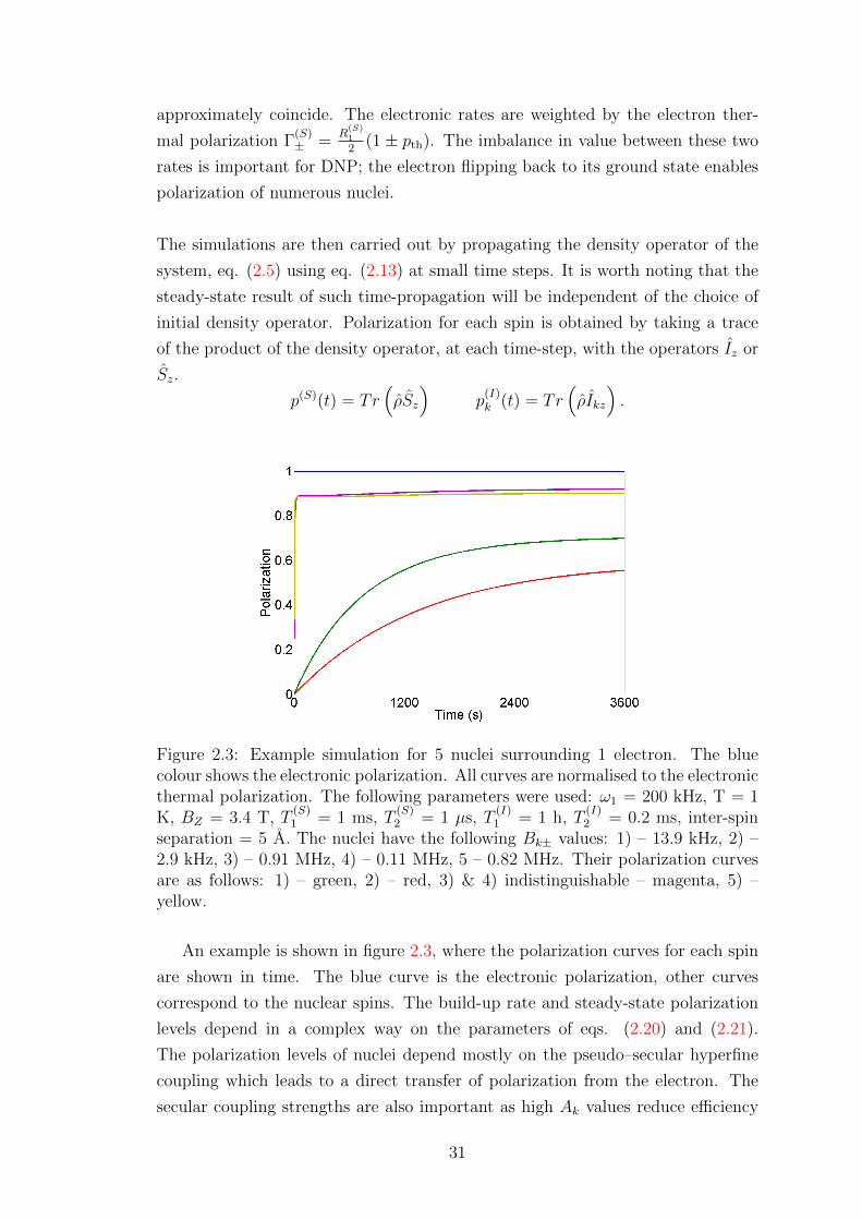
approximately coincide. The electronic rates are weighted by the electron ther-

mal polarization Γ(S)± =

R(S)1

2(1 ± pth). The imbalance in value between these two

rates is important for DNP; the electron flipping back to its ground state enables

polarization of numerous nuclei.

The simulations are then carried out by propagating the density operator of the

system, eq. (2.5) using eq. (2.13) at small time steps. It is worth noting that the

steady-state result of such time-propagation will be independent of the choice of

initial density operator. Polarization for each spin is obtained by taking a trace

of the product of the density operator, at each time-step, with the operators Iz or

Sz.

p(S)(t) = Tr(ρSz

)p

(I)k (t) = Tr

(ρIkz

).

Figure 2.3: Example simulation for 5 nuclei surrounding 1 electron. The bluecolour shows the electronic polarization. All curves are normalised to the electronicthermal polarization. The following parameters were used: ω1 = 200 kHz, T = 1K, BZ = 3.4 T, T

(S)1 = 1 ms, T

(S)2 = 1 µs, T

(I)1 = 1 h, T

(I)2 = 0.2 ms, inter-spin

separation = 5 A. The nuclei have the following Bk± values: 1) – 13.9 kHz, 2) –2.9 kHz, 3) – 0.91 MHz, 4) – 0.11 MHz, 5 – 0.82 MHz. Their polarization curvesare as follows: 1) – green, 2) – red, 3) & 4) indistinguishable – magenta, 5) –yellow.

An example is shown in figure 2.3, where the polarization curves for each spin

are shown in time. The blue curve is the electronic polarization, other curves

correspond to the nuclear spins. The build-up rate and steady-state polarization

levels depend in a complex way on the parameters of eqs. (2.20) and (2.21).

The polarization levels of nuclei depend mostly on the pseudo–secular hyperfine

coupling which leads to a direct transfer of polarization from the electron. The

secular coupling strengths are also important as high Ak values reduce efficiency

31

of polarization transport. Nuclei with the high Bk± values reach high polarization

values (nuclei 3,4,5). Nuclei 1 and 2 reach lower polarization levels due to weaker

pseudo–secular coupling, however the relatively strong dipolar coupling to the

remaining nuclei leads to these two still having a decent polarization level. Nuclei

3 and 4 have a very strong dipolar coupling of ∼ 1 kHz hence equalise making

their polarization curves indistinguishable. It is expected that as time → ∞, the

nuclear polarizations would all equalise.

2.3 Theory of cross effect DNP

This section focuses on the theory of CE-DNP on a microscopic scale. This mech-

anism is most pronounced at temperatures of a few tens of Kelvin, typically in the

region of liquid nitrogen temperature, and is most relevant to bi-radical solutions

or mono-radical solutions of higher concentrations. This is currently the most ef-

ficient of the DNP mechanisms. It requires significant inhomogeneous broadening

of the electron EPR line, and the dipolar interaction strength between the elec-

trons should be relatively strong. This chapter will be focused on the static case

of CE-DNP for a simple case of two electron radicals surrounded by nuclear spins.

2.3.1 Cross effect

The cross effect mechanism is a three-spin process, acting between two electrons

and a nucleus. There is strong coupling between the two electrons, and the elec-

tron pairs are usually found in the form of bi-radical molecules or mono-radical

molecules in close proximity. For this mechanism to be dominant, the inhomo-

geneous broadening (η) of the EPR spectrum should be greater than the nuclear

Larmor frequency (ωI). The homogeneous broadening (ζ) on the other hand

should be less than the nuclear Larmor frequency; η > ωI > ζ. With a greater

inhomogeneous broadening, a higher number of electron pairs where the differ-

ence between their Larmor frequencies matches the CE-DNP resonance condition,

would likely be encountered.

32

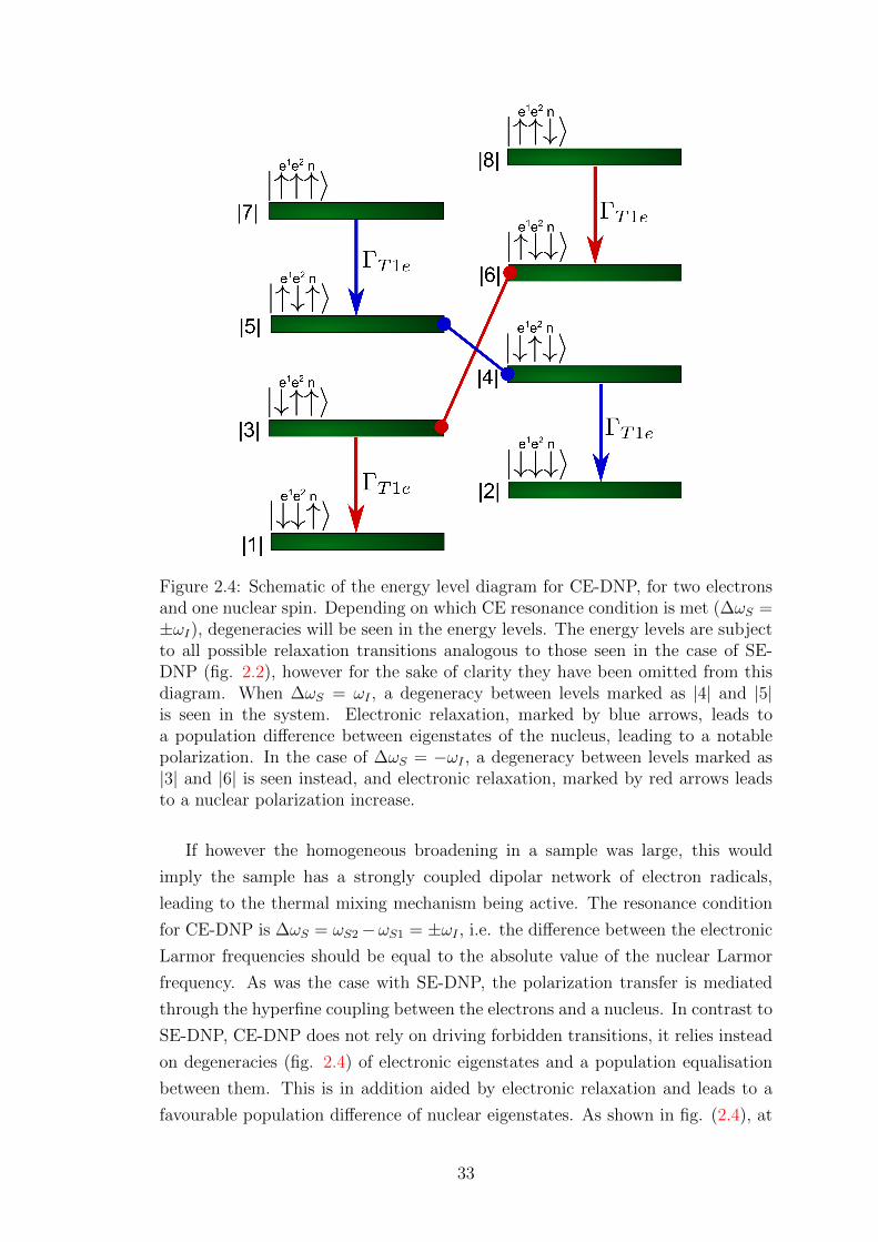
Figure 2.4: Schematic of the energy level diagram for CE-DNP, for two electronsand one nuclear spin. Depending on which CE resonance condition is met (∆ωS =±ωI), degeneracies will be seen in the energy levels. The energy levels are subjectto all possible relaxation transitions analogous to those seen in the case of SE-DNP (fig. 2.2), however for the sake of clarity they have been omitted from thisdiagram. When ∆ωS = ωI , a degeneracy between levels marked as |4| and |5|is seen in the system. Electronic relaxation, marked by blue arrows, leads toa population difference between eigenstates of the nucleus, leading to a notablepolarization. In the case of ∆ωS = −ωI , a degeneracy between levels marked as|3| and |6| is seen instead, and electronic relaxation, marked by red arrows leadsto a nuclear polarization increase.

If however the homogeneous broadening in a sample was large, this would

imply the sample has a strongly coupled dipolar network of electron radicals,

leading to the thermal mixing mechanism being active. The resonance condition

for CE-DNP is ∆ωS = ωS2−ωS1 = ±ωI , i.e. the difference between the electronic

Larmor frequencies should be equal to the absolute value of the nuclear Larmor

frequency. As was the case with SE-DNP, the polarization transfer is mediated

through the hyperfine coupling between the electrons and a nucleus. In contrast to

SE-DNP, CE-DNP does not rely on driving forbidden transitions, it relies instead

on degeneracies (fig. 2.4) of electronic eigenstates and a population equalisation

between them. This is in addition aided by electronic relaxation and leads to a

favourable population difference of nuclear eigenstates. As shown in fig. (2.4), at

33

the resonance condition ∆ωS = ωI the states numbered as |4| and |5|, linked in the

diagram by a blue line, become degenerate, and the populations of those states will

equalise. Electronic relaxation pathways for the second electron (marked by blue

arrows) lead to the depopulation of states |7|, then |4| and |5|, causing an increased

population of state |2|, thus resulting in a large population difference between the

nuclear eigenstates, and resulting in nuclear state |↓〉 being more populated. At

the resonance condition ∆ωS = −ωI the states numbered as |3| and |6|, linked in

the diagram by a red line, become degenerate, and the populations of those states

will equalise. Electronic relaxation pathways for the second electron (marked by

red arrows) lead to the depopulation of states |8|, then |3| and |6|, leading to an

increased population of state |1|, thus causing a large population difference of the

nuclear eigenstates, and resulting in the nuclear state |↑〉 being populated.

2.3.2 Hamiltonian

The microscopic model is based on an electron pair surrounded by nuclear spins.

The Hamiltonian is analogous to that seen in SE-DNP, eq. (2.16), with the addi-

tion of an electronic dipolar coupling term

H = HZ + HSS + HIS + HII + Hmw. (2.22)

In the presence of a magnetic field, each spin has a Zeeman energy resulting in

the Zeeman Hamiltonian of the system

HZ = ω(1)S S(1)

z + ω(2)S S(2)

z + ωI∑k

Ikz.

The cross effect mechanism relies on each electron having a different g-anisotropy

[23] (introduction chapter), leading to a significant difference in their Larmor

frequencies. The mechanism is most efficient when the difference between the

Larmor frequencies of the two electrons is approximately equal to the nuclear

Larmor frequency∣∣∣ω(1)

S − ω(2)S

∣∣∣ ≈ ωI . The electronic dipolar coupling present in

the system is crucial for the mechanism to function, it allows the energy levels to

become degenerate, as described in chapter 1. The form of the dipolar coupling

is analogous to the dipolar coupling between nuclear spins. In the presence of a

magnetic field, the dipolar Hamiltonian has the secular form

HSS = D

(2S(1)

z S(2)z −

1

2S

(1)+ S

(2)− −

1

2S

(1)− S

(2)+

),

34

where the coupling parameter D is

−µ0

4π

γ(S1)γ(S2)~2R3

(3 cos(ΘS)− 1) .

The angle ΘS is the angle between the vector joining the electron spins, and the

magnetic field vector BZ . The parameter D is maximised for a given separation

R, when ΘS = 0◦ or 180◦, i.e. the vector joining the two spins is parallel or

anti-parallel to BZ . The secular, electronic dipolar Hamiltonian is invariant un-

der rotation, therefore it is unaltered when proceeding to the rotating frame of

reference of the microwave radiation. The nuclear dipole-dipole Hamiltonian is

identical to the SE-DNP case. The hyperfine, and microwave Hamiltonians are

also analogous extensions to the SE-DNP case; each electron is influenced by the

microwave field, and each electron has hyperfine coupling to surrounding nuclei.

In the presence of microwave radiation it is necessary to proceed to the rotating

frame of reference, as described in section 2.2.3.

2.3.3 CE-DNP master equation

The rotating frame of reference CE-DNP Hamiltonian is written as

H = ∆1S(1)z + ∆2S

(2)z +

∑k

ωI Ikz +D

(2S(1)

z S(2)z −

1

2S

(1)+ S

(2)− −

1

2S

(1)− S

(2)+

)+∑j

∑k

(A

(j)k Ikz +B

(j)k+Ik+ +B

(j)k−Ik−

)S(j)z

+∑kk′

dkk′

(2Ikz Ik′z −

1

2Ik+Ik′− −

1

2Ik−Ik′+

)+ω1

2

(S

(1)+ + S

(1)− + S

(2)+ + S

(2)−

).

(2.23)

The parameters ∆1,∆2 are the offset terms for each electron. The CE-DNP mecha-

nism is most efficient when one of the electrons is on-resonance with the microwave

radiation, and the other electron is at an offset of ±ωI ; ∆1 ≈ 0, ∆2 ≈ ±ωI . This

leads to the degeneracies in energy levels of the system, combined with relaxation

resulting in polarization enhancements of the surrounding nuclei. In the case of

cross effect DNP, the enhancement scales with magnetic field strength as B−1Z ,

this is most likely related to the fact that the separation between energy levels

increases linearly with increasing field strength.

The dissipator contains all the terms that are present in SE-DNP, eq. (2.21). In

addition, processes of both longitudinal and transverse cross-relaxation are possi-

ble between the electron pair due to the action of the environment. These have

35

the form

Γ(SS)+− D

[S

(1)+ S

(2)−

]+ Γ

(SS)−+ D

[S

(1)− S

(2)+

]for londitudinal cross-relaxation, and

Γ(SS)z D

[S(2)z − S(1)

z

],

for transverse cross-relaxation. The CE-DNP system dissipator is then

Γ(S1)+ D

[S

(1)+

]+ Γ

(S1)− D

[S

(1)−

]+ Γ(S1)

z D[S(1)z

]+ Γ

(S2)+ D

[S

(2)+

]+Γ

(S2)− D

[S

(2)−

]+ Γ(S2)

z D[S(2)z

]+ Γ

(SS)+− D

[S

(1)+ S

(2)−

]+ Γ

(SS)−+ D

[S

(1)− S

(2)+

]+Γ(SS)

z D[S(2)z − S(1)

z

]+∑k

Γ(I)k+D [Ik+] + Γ

(I)k−D [Ik−] + Γ

(I)kz D [Ikz] . (2.24)

As previously mentioned, the terms corresponding to rates Γ(I)kz ,Γ

(S1)z ,Γ

(S2)z are re-

sponsible for modelling decoherence of nuclear spins and electrons, respectively.

Since the nuclear thermal polarization is very low, even at temperatures ap-

proaching 1K, the rates Γ(I)k+,Γ

(I)k− approximately coincide. The electronic rates

are weighted by the electron thermal polarization Γ(Sj)± =

R(S)1

2(1 ± pth). The sys-

tem density operator is propagated using eqs. 2.13, 2.23, 2.24. Polarization for

each spin is then obtained by taking a trace of the product of the density operator

at each time-step and Iz or S(j)z operator

p(Sj)(t) = Tr(ρS(j)

z

)p

(I)k (t) = Tr

(ρIkz

).

2.4 Adiabatic elimination

The work in this chapter follows the original derivation by A. Karabanov, and has

been previously published by us in [52].

As discussed in section 2.1.1, the density operator dimension in DNP, or in fact any

quantum-mechanical simulations, scales as 4n, for n system constituents. Such un-

favourable scaling limits simulations of spin systems to just a few spins. To date,

systems with up to 10 spins [37] have been successfully simulated without any

approximations. Any system larger than this would require very large amounts of

memory, which is expensive and not feasible for wide-spread regular use.

There exist mathematical techniques that allow reduction of the effective sub-

space of the density operator, one such technique is called adiabatic elimination

[50]. The method of adiabatic elimination allows for separating subspaces of the

36

density operator which evolve on different time-scales, such that slow dynamics

can be separated from fast dynamics. In the context of quantum mechanics this

process is somewhat analogous to proceeding to the rotating frame of reference,

and the approximations that are taken to derive the Lindblad master equation in

section 2.1.3, where the environment is assumed to evolve on a time-scale that is

much faster than the time-scale over which the system evolves, hence the system

dynamics are coarse grained.

In a simplified example, this can be illustrated by two coupled differential equa-

tions

L0 = A · L0 +B · L1

L1 = C · L0 +D · L1,

where L0 represents the system, coupled to a rapidly–evolving environment (L1),

and A,B,C,D are linear coefficients. Approximate effective dynamics are found

for the system involving a mean, coarse-grained effect of the environment on the

system. In the case of adiabatic elimination applied to DNP we separate slow

dynamics of the the density operator from the fast ones.

2.4.1 Mathematical procedure

The purpose of the adiabatic elimination is to separate the slow L0, and the fast

dynamics L1

ρ = Lρ = (L0 + L1) ρ.

For any linear system with constant coefficients

˙ρ = Lρ,

defined in Hilbert space H, we are interested in a reduced dimensions subspace

H0 ⊂ H.

Using Nakajima-Zwanzig projection operators [50], where P is the projector onto

the subspace of interest (H0), Q is the complementary projector, we are effectively

looking at the space decomposition H = H0 +H1,

(P +Q) ρ = (P +Q) L (P +Q) ρ

(P +Q) ρ = (PLP + PLQ+QLP +QLQ) ρ

P ρ = (PLP + PLQ) ρ

Qρ = (QLQ+QLP) ρ

37

defining now

L00 = PLP L01 = PLQ

L11 = QLQ L10 = QLP ,

two coupled differential equations are formed

˙ρ0 = L00ρ0 + L01ρ1 (2.25)

˙ρ1 = L11ρ1 + L10ρ0. (2.26)

The general solution to eq. (2.26) with respect to ρ1, in time is

ρ1 (t) = eL11tρ1 (0) + eL11t

∫ t

0

e−L11τL10ρ0 (τ) dτ,

where frequently the boundary condition ρ1 (0) = Qρ = 0 will usually apply.

Substituting into eq. (2.25), dynamics enclosed in H0 are obtained

˙ρ0 = L00ρ0 +

∫ t

0

L01eL11(t−τ)L10ρ0 (τ) dτ

˙ρ0 = L00ρ0 +

∫ t

0

K(t− τ)ρ0 (τ) dτ. (2.27)

The three-part product here is the kernel:

K(t− τ) = L01eL11(t−τ)L10.

The Laplace transform of both sides of equation 2.27 is taken; both sides are

multiplied by e−εt, and integrated between 0 and ∞ with respect to t.

LHS

Integration by parts is used ∫u′v = uv −

∫v′u

∫ ∞0

e−εt ˙ρ0 (t) dt = ρ0(t)e−εt∣∣∞0−∫ ∞

0

−ε e−εtρ0(t)dt = −ρ0(0) + ε

∫ ∞0

e−εtρ0(t)dt.

38

RHS

−ρ0(0) + ε

∫ ∞0

ρ0(t)dt =

∫ ∞0

e−εtL00ρ0 +

∫ ∞0

∫ t

0

e−εtK (t− τ) ρ0 (τ) dτdt.

In principle, the kernel can be written in a diagonalised frame in which it acts

as a sum of eigenfunctions. This could be achieved by writing L11 in a diagonal

basis. Analytically this would be difficult, even for a 2-spin problem, however in

principle there exists such diagonal form:

K(t− τ) ≡∑k

Kkeεk(t−τ).

The kernel term has the form of a convolution function. As with the Fourier

Transform, a Laplace Transform of a convolution function is the product of the

individual functions in the space of eigenvalues. Thus∫ ∞0

∫ t

0

e−εtK (t− τ) ρ0 (τ) dτdt = lK (ε) · lρ0 (ε) .

Proof

∫ ∞0

e−εt(∫ t

0

K(t− τ)ρ0(τ)dτ

)dt =

∑k

∫ ∞0

e(εk−ε)t(∫ t

0

e−ετKkρ0(τ)dτ

)dt

this is integrated by parts, to find a bound solution, defining for clarity

u =e(εk−ε)t

εk − εu′ = e(εk−ε)t v =

∑k

∫ t

0

e−ετKkρ0(τ)dτ

v′ =∑k

(e−εktKkρ0(t) · d

dtt− e0Kkρ0(0) · d

dt0 +

∫ t

0

∂

∂te−ετKkρ0(τ)

). . .

v′ =∑k

(e−εktKkρ0(t)

),

where for v′ a standard mathematical property concerning derivation of integrals

is used.

uv =

[∑k

e(εk−ε)t

εk − ε

∫ t

0

e−εkτKkρ0(τ)dτ

]t=∞t=0

= . . .

=∑k

e(εk−ε)∞

εk − ε

∫ ∞0

e−εkτKkρ0(τ)dτ −∑k

1

εk − ε

∫ 0

0

e−εkτKkρ0(τ)dτ = 0.

39

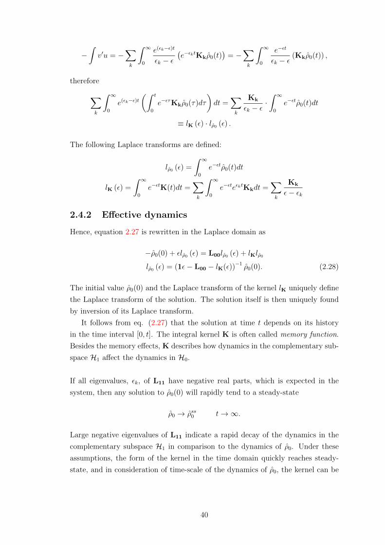
−∫v′u = −

∑k

∫ ∞0

e(εk−ε)t

εk − ε(e−εktKkρ0(t)

)= −

∑k

∫ ∞0

e−εt

εk − ε(Kkρ0(t)) ,

therefore

∑k

∫ ∞0

e(εk−ε)t(∫ t

0

e−ετKkρ0(τ)dτ

)dt =

∑k

Kk

εk − ε·∫ ∞

0

e−εtρ0(t)dt

≡ lK (ε) · lρ0 (ε) .

The following Laplace transforms are defined:

lρ0 (ε) =

∫ ∞0

e−εtρ0(t)dt

lK (ε) =

∫ ∞0

e−εtK(t)dt =∑k

∫ ∞0

e−εteεktKkdt =∑k

Kk

ε− εk

2.4.2 Effective dynamics

Hence, equation 2.27 is rewritten in the Laplace domain as

−ρ0(0) + εlρ0 (ε) = L00lρ0 (ε) + lKlρ0

lρ0 (ε) = (1ε− L00 − lK(ε))−1 ρ0(0). (2.28)

The initial value ρ0(0) and the Laplace transform of the kernel lK uniquely define

the Laplace transform of the solution. The solution itself is then uniquely found

by inversion of its Laplace transform.

It follows from eq. (2.27) that the solution at time t depends on its history

in the time interval [0, t]. The integral kernel K is often called memory function.

Besides the memory effects, K describes how dynamics in the complementary sub-

space H1 affect the dynamics in H0.

If all eigenvalues, εk, of L11 have negative real parts, which is expected in the

system, then any solution to ρ0(0) will rapidly tend to a steady-state

ρ0 → ρss0 t→∞.

Large negative eigenvalues of L11 indicate a rapid decay of the dynamics in the

complementary subspace H1 in comparison to the dynamics of ρ0. Under these

assumptions, the form of the kernel in the time domain quickly reaches steady-

state, and in consideration of time-scale of the dynamics of ρ0, the kernel can be

40

integrated to infinity∫ ∞0

K(t) =∑k

Kk

∫ ∞0

eεktdt =∑k

Kk

[eεkt

εk

]∞0

= −∑k

Kk

εk≡ −L01L11

−1L10.

We assume the dynamics in the subspace ρ1 to evolve rapidly, and quickly be

’forgotten’ by the system in the subspace ρ0, thus we require

max(eig(L01,L10)� min(εk), (2.29)

and hence we work in a regime where the eigenvalues of the effective system are

small

ε� min(εk)

i.e. slow dynamics in the subspace H0.

Mathematically, the Laplace Transform of the kernel function

lK(ε) =∑k

Kk

ε− εk

is expanded around ε ≈ 0, i.e. the region of slower dynamics with small eigenval-

ues, so in result we have the Maclaurin series

lK (ε) ≈ lK(0) +∂lK(0)

∂ε(ε) +

∂2lK(0)

∂ε2(ε2/2

)+ . . . .

If ||L01|| · ||L10|| � ε2k then

−∂lK(0)

∂ε(ε) = −

∑k

Kk

ε2k≈ 0

and hence

lK(ε) ≈ lK(0) = −∑k

Kk

εk.

The effect of lK(0) can be rewritten as a superoperator M. An inverse Laplace

transform is then applied to obtain the solution eq. (2.28) in the time-domain

lρ0 (ε) = (1ε− L00 −M)−1 ρ0(0). (2.30)

Since the Laplace transform of a function f(t) = eαt is F (ε) = 1ε−α , the Laplace

inverse of eq. 2.30 is

ρ0(t) = e(L00+M)tρ0(0),

41

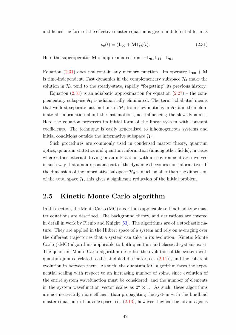
and hence the form of the effective master equation is given in differential form as

˙ρ0(t) = (L00 + M) ρ0(t). (2.31)

Here the superoperator M is approximated from −L01L11−1L01.

Equation (2.31) does not contain any memory function. Its operator L00 + M

is time-independent. Fast dynamics in the complementary subspace H1 make the

solution in H0 tend to the steady-state, rapidly “forgetting” its previous history.

Equation (2.31) is an adiabatic approximation for equation (2.27) – the com-

plementary subspace H1 is adiabatically eliminated. The term ’adiabatic’ means

that we first separate fast motions in H1 from slow motions in H0 and then elim-

inate all information about the fast motions, not influencing the slow dynamics.

Here the equation preserves its initial form of the linear system with constant

coefficients. The technique is easily generalised to inhomogeneous systems and

initial conditions outside the informative subspace H0.

Such procedures are commonly used in condensed matter theory, quantum

optics, quantum statistics and quantum information (among other fields), in cases

where either external driving or an interaction with an environment are involved

in such way that a non-resonant part of the dynamics becomes non-informative. If

the dimension of the informative subspace H0 is much smaller than the dimension

of the total space H, this gives a significant reduction of the initial problem.

2.5 Kinetic Monte Carlo algorithm

In this section, the Monte Carlo (MC) algorithms applicable to Lindblad-type mas-

ter equations are described. The background theory, and derivations are covered

in detail in work by Plenio and Knight [53]. The algorithms are of a stochastic na-

ture. They are applied in the Hilbert space of a system and rely on averaging over

the different trajectories that a system can take in its evolution. Kinetic Monte

Carlo (kMC) algorithms applicable to both quantum and classical systems exist.

The quantum Monte Carlo algorithm describes the evolution of the system with

quantum jumps (related to the Lindblad dissipator, eq. (2.11)), and the coherent

evolution in between them. As such, the quantum MC algorithm faces the expo-

nential scaling with respect to an increasing number of spins, since evolution of

the entire system wavefunction must be considered, and the number of elements

in the system wavefunction vector scales as 2n × 1. As such, these algorithms

are not necessarily more efficient than propagating the system with the Lindblad

master equation in Liouville space, eq. (2.13), however they can be advantageous

42

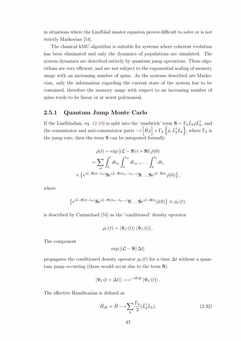
in situations where the Lindblad master equation proves difficult to solve or is not

strictly Markovian [54].

The classical kMC algorithm is suitable for systems where coherent evolution

has been eliminated and only the dynamics of populations are simulated. The

system dynamics are described entirely by quantum jump operations. These algo-

rithms are very efficient, and are not subject to the exponential scaling of memory

usage with an increasing number of spins. As the systems described are Marko-

vian, only the information regarding the current state of the system has to be

contained, therefore the memory usage with respect to an increasing number of

spins tends to be linear or at worst polynomial.

2.5.1 Quantum Jump Monte Carlo

If the Lindbladian, eq. (2.10) is split into the ’sandwich’ term S = ΓkLkρL†k, and

the commutator and anti-commutator parts −i[Hρ]

+ Γk

{ρ, L†kLk

}, where Γk is

the jump rate, then the term S can be integrated formally

ρ(t) = exp [(L − S) t+ St] ρ(0)

=∑m

∫ t

0

dtm

∫ tm

0

dtm−1 . . .

∫ t2

0

dt1

×{e(L−S)(t−tm)Se(L−S)(tm−tm−1)S . . .Se(L−S)t1 ρ(0)

},

where

{e(L−S)(t−tm)Se(L−S)(tm−tm−1)S . . .Se(L−S)t1 ρ(0)

}≡ ρC(t),

is described by Carmichael [55] as the ’conditioned’ density operator

ρC(t) = |ΨC(t)〉 〈ΨC(t)| .

The component

exp [(L − S) ∆t]

propagates the conditioned density operator ρC(t) for a time ∆t without a quan-

tum jump occurring (those would occur due to the term S):

|ΨC(t+ ∆t)〉 = e−iH∆t |ΨC(t)〉 .

The effective Hamiltonian is defined as

Heff = H − i∑k

Γk2

(L†kLk), (2.32)

43

and is derived from L − S. At a time when a quantum jump occurs, the jump

operator corresponding to that jump is applied to the wavefunction

|ΨC(t)〉′ = Lk |ΨC(t)〉 .

Implementation

The implementation of the algorithm for quantum MC relies on the following

steps:

1. The probabilities for all possible quantum jumps are calculated

∆Pk = Γkδt 〈Ψ| L†kLk |Ψ〉

2. A random number r1 is obtained, where 0 < r1 ≤ 1

3. If r1 <∑

k ∆Pk, a quantum jump will occur.

3.1. Draw a second random number r2 to choose which jump will occur,

select rate corresponding to jump where

r2 <

∑k1 ∆Pk∑

∆P (∀k)

4. Otherwise if r1 >∑

k ∆Pk, no quantum jump will occur, and the system

evolves under the influence of the non-Hermitian effective Hamiltonian, eq.

(2.32)

|Ψ〉 →

{1− iHeff∆t

}|Ψ〉

(1−∑

∆Pk)1/2

5. Steps 1-4 are repeated until a desired time t is reached, to form an individual

trajectory

6. Trajectories are averaged to approximate the time evolution of observables

of interest.

2.5.2 Classical kinetic Monte Carlo

If the coherent evolution is eliminated, then the system dynamics are restricted

to the populations, and are described entirely by jumps occurring in the system.

These are described by terms of S. Only knowledge of the current eigenstate of

each system constituent needs to be known, in order to propagate the system in

time and form a system trajectory. Since the form of the jump operators is known,

44

the associated rates connect classical system configurations. No re-normalisation

of the system state is required.

The fixed time-step kMC algorithm can be summarised in the following steps

1. The effective rates, Γk, associated with the jump operations are calculated

2. Two uniformly-distributed random numbers r1, r2 are generated

3. A jump will be implemented in the system if

r1 > e−∑k ∆t,

otherwise steps 2-3 are repeated

4. The effective rates are normalised in a vector, so that their cumulative sum

adds to 1. A rate is then selected for which the normalised rate value is

greater than the second random number r2, i.e. one finds the rate for which

r2 <

∑k=i1 Γk∑

k Γk (∀k),

the corresponding jump operation is then carried out

5. Steps 1-4 are repeated until a desired time τ is reached, to form a single

trajectory of the system

6. Trajectories are averaged to approximate the time evolution of observables

of interest.

The above algorithm relies on selecting an appropriate time step, and may be

inefficient in cases where the time-step selected is too small. In such case, steps

2-3 would frequently be repeated with no jumps occurring in the system. If the

time-step selected is too large, the dynamics might be under-sampled, and thus

inaccurate. This would be the case if only one jump operation is carried out within

a current time-step where numerous jumps should have been implemented.

Variable time-step kMC

A variable time-step kMC algorithm avoids the issues outlined above. Step 3 in

the above algorithm is altered by setting r1 = e−∑k ∆t. The equation is rearranged

to find the time step required between each jump operation in the system

∆t =− log r1∑

k Γk.

45

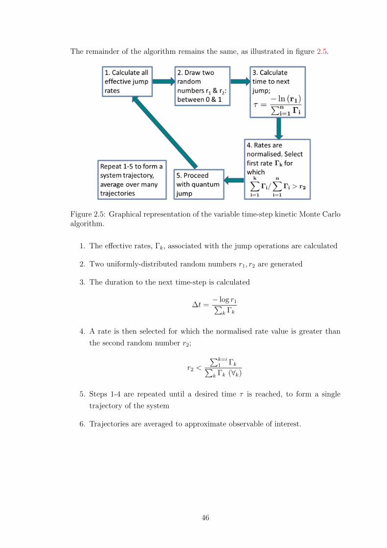
The remainder of the algorithm remains the same, as illustrated in figure 2.5.

Figure 2.5: Graphical representation of the variable time-step kinetic Monte Carloalgorithm.

1. The effective rates, Γk, associated with the jump operations are calculated

2. Two uniformly-distributed random numbers r1, r2 are generated

3. The duration to the next time-step is calculated

∆t =− log r1∑

k Γk

4. A rate is then selected for which the normalised rate value is greater than

the second random number r2;

r2 <

∑k=i1 Γk∑

k Γk (∀k)

5. Steps 1-4 are repeated until a desired time τ is reached, to form a single

trajectory of the system

6. Trajectories are averaged to approximate observable of interest.

46

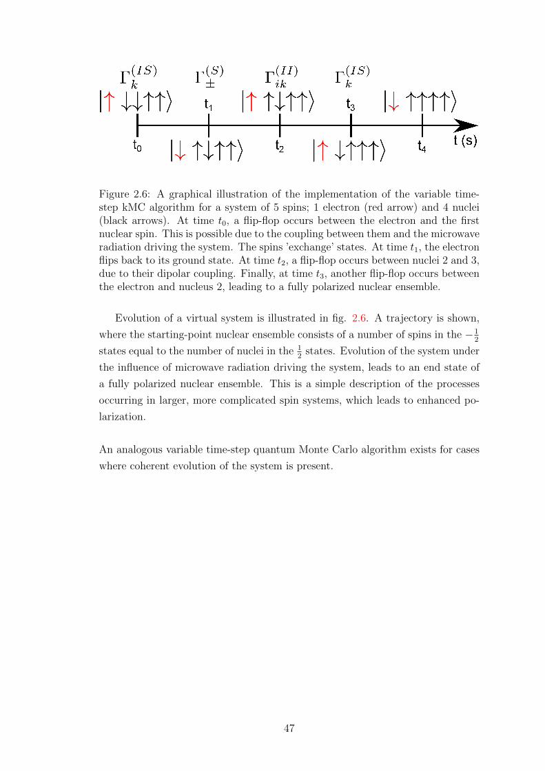
Figure 2.6: A graphical illustration of the implementation of the variable time-step kMC algorithm for a system of 5 spins; 1 electron (red arrow) and 4 nuclei(black arrows). At time t0, a flip-flop occurs between the electron and the firstnuclear spin. This is possible due to the coupling between them and the microwaveradiation driving the system. The spins ’exchange’ states. At time t1, the electronflips back to its ground state. At time t2, a flip-flop occurs between nuclei 2 and 3,due to their dipolar coupling. Finally, at time t3, another flip-flop occurs betweenthe electron and nucleus 2, leading to a fully polarized nuclear ensemble.

Evolution of a virtual system is illustrated in fig. 2.6. A trajectory is shown,

where the starting-point nuclear ensemble consists of a number of spins in the −12

states equal to the number of nuclei in the 12

states. Evolution of the system under

the influence of microwave radiation driving the system, leads to an end state of

a fully polarized nuclear ensemble. This is a simple description of the processes

occurring in larger, more complicated spin systems, which leads to enhanced po-

larization.

An analogous variable time-step quantum Monte Carlo algorithm exists for cases

where coherent evolution of the system is present.

47

Chapter 3

Solid Effect

3.1 Adiabatic elimination of Solid Effect dynam-

ics

This chapter is focused on the derivation of the effective dynamics governing SE–

DNP with the use of projection operators. This is followed by: a description of the

derived effective rates and a comprehensive error analysis, spin diffusion studies

in 1D systems, large spin ensemble simulations, fitting of the polarization curves,

and finally scaling of the error and computational time with respect to the system

size. Research described in this chapter is described in our publication [52].

3.1.1 Elimination of non–zero quantum coherences

The SE–DNP dynamics are projected onto the diagonal part of the density opera-

tor, the so–called Zeeman subspace, in a two–step process. The dynamics are first

projected onto the zero–quantum subspace, and subsequently the Zeeman sub-

space of the zero–quantum subspace. In effect, the relevant subspace dimension

of the density operator is reduced from 4(n+1) to 2(n+1) for n nuclear spins. The

mathematical procedure of adiabatic elimination is explained in section 2.4.

The SE–DNP Hamiltonian for a single electron and n nuclei is shown in eq. (2.20).

For convenience, the rotating–frame of reference Hamiltonian can be separated into

48

four parts

HZ = ∆Sz +∑k

Ikz

H0 = λSz +∑k

AkSz Ikz +ω1

2(S+ + S−)

+dkk′∑kk′

(2Ikz Ik′z −1

2Ik+Ik′− −

1

2Ik−Ik′+)

H± =∑k

Bk±Sz Ik±.

The terms HZ , H0 keep dynamics of a particular subspace enclosed in that sub-

space. Terms H±, on the other hand, cause cross–overs between the different

subspaces. At the SE resonance condition of either ∆ = ±ωI , the Zeeman Hamil-

tonian becomes HZ = ωI(±Sz +∑

k Ikz).

The system is also subject to dissipation. There is longitudinal relaxation (T1)

driving all spins back to their thermal equilibrium, as well as decoherence (T2)

processes. The dissipator for this system is written as

Γ = Γ(S)+ D[S+] + Γ

(S)− D[S−] + Γ(S)

z D[Sz]

+∑k

(Γ

(I)k+D[Ik+] + Γ

(I)k−D[Ik−] + Γ

(I)kz D[Ikz]

),

with associated rates

Γ(S)± =

R(S)1

2(1∓ pth) Γ(S)

z = 2R(S)2

Γ(I)k+ = Γ

(I)k− =

R(I)1

2Γ

(I)kz = 2R

(I)2 . (3.1)

As outlined in section 2.1.3, the system dynamics are then described by

˙ρ = (−i ˆH + Γ)ρ. (3.2)

The Liouville state space can be decomposed as

L =∑Lq,

where Lq is the subspace of q–quantum coherences,

ˆHZ ρ = qωI ρ, ρ ∈ Lq, q = 0, ±1, . . . , ±(n+ 1). (3.3)

49

The case of q = 0, i.e. when ˆHZ ρ = 0 denotes the zero–quantum subspace.

The subspace of interest is therefore the one that commutes with the Zeeman

Hamiltonian. The dynamics in this subspace are a lot slower than the dynamics

in the other subspaces, since

ωI � Ak, Bk±, dkk′ ,Γ(S)z ,Γ

(S)± ,Γ

(I)kz ,Γ

(I)k±, (3.4)

at high field, meaning the separation of these subspaces using adiabatic elimination

is appropriate.

For a simple two–spin system, the density operator is

ρ = ρe ⊗ ρn =

(a(Sz + 1

2) cS+

c∗S− b(Sz − 12)

)⊗

(d(Iz + 1

2) eI+

e∗I− f(Iz − 12)

)= ...

where a, b, c, d, e, f are linear coefficients. The elements of the zero–quantum sub-space of the density operator are then easily written out

α1

(Sz + 1

2

) (Iz + 1

2

)α2

(Sz + 1

2

)I+ α3S+

(Iz + 1

2

)α4S+I+

α5

(Sz + 1

2

)I− α6

(Sz + 1

2

) (Iz − 1

2

)α7S+I− α8S+

(Iz − 1

2

)α9S−

(Iz + 1

2

)α10S−I+

(α11Sz − 1

2

) (Iz + 1

2

)α12

(Sz − 1

2

)I+

α13S−I− α14

(Iz − 1

2

)S− α15

(Sz − 1

2

)I− α16

(Sz − 1

2

) (Iz − 1

2

) . (3.5)

Here elements existing in the zero–quantum subspace are marked in red, and for

convenience 12

is used to denote the identity matrix divided by 2. The symbols αj

(1 ≤ j ≤ 16) denote linear coefficients.

Letting the subspace H0 be the zero–quantum subspace, and H1 the complimen-

tary subspace

H0 = L0, H1 =∑q 6=0

Lq,

the relations

(−i ˆH0 + Γ)Lq ⊂ Lq, ˆH± Lq ⊂ Lq±1

along with (3.3) give the following properties

L00ρ0 = −i ˆH0 + Γρ0, L10ρ0 = −i( ˆH+ + ˆH−)ρ0,

L01L±1 = −i ˆH∓ L±1, L01Lq = 0, |q| > 1,

L11L±1 = −(±iωI1 + i ˆH0 + i ˆH± − Γ)L±1,

L11Lq = −(iqωI1 + i ˆH0 + i ˆH+ + i ˆH− − Γ)Lq, |q| > 1.

(3.6)

Due to the presence of relaxation, the eigenvalues of the superoperator L11 have

negative real parts, ζ−, thus the solution in H1 rapidly tends to a steady–state.

Therefore, the condition outlined in section 2.4 is satisfied, and the Kernel func-

tion is well approximated by its time–independent steady–state form. The zero–

50

quantum master equation is well approximated by

˙ρ0 = (L00 + M) ρ0,

and M ≡ −L01L−111 L10.

3.1.2 Superoperator M

In order to find the explicit form of M the properties of superoperators summarised

in eq. (3.6) were used. Superoperator L01 acting on ρ0 leaves the dynamics in the

first quantum coherence subspace L±1

L10ρ0 = −i( ˆH+ + ˆH−)ρ0.

Letting X = L−111 L10ρ0, it is clear that

L11X = L10ρ0 = −i(

ˆH+ + ˆH−

)ρ0.

Therefore, since ωI � (H0,±,D), X can be expanded as a rapidly–converging

power series, truncated to second order

X =x(1)

ωI+x(2)

ωI 2+ 0

(x(3)

ωI 3

).

Each term in the series expansion of X can also be separated according to the

coherence subspace order. We have from eq. (3.6)

L11L±1 = −(±iωI1 + i ˆH0 + i ˆH± − Γ

)L±1,

L11Lq (|q| > 1) = −(±iqωI1 + i ˆH0 + i ˆH+ + i ˆH− − Γ

)Lq,

hence only focusing on coherence subspaces up to q = 2

L11X = −(iωI1 + (i ˆH0 − Γ) + i ˆH+

)X+1,

−(−iωI1 + (i ˆH0 − Γ) + i ˆH−

)X−1,

−(

2iωI1 + (i ˆH0 − Γ) + i ˆH+ + i ˆH−

)X+2,

−(−2iωI1 + (i ˆH0 − Γ) + i ˆH− + i ˆH−

)X−2,

51

≡ −i(

ˆH+ + ˆH−

)ρ0.

The equations can then be rewritten according to coherence order

−(iωIX+1 + (i ˆH0 − Γ)X+1 + i ˆH−X+2

)= −i ˆH+ρ0, (3.7)

−(−iωIX−1 + (i ˆH0 − Γ)X−1 + i ˆH+X−2

)= −i ˆH−ρ0, (3.8)

−(

2iωIX+2 + (i ˆH0 − Γ)X+2 + i ˆH+X+1

)= 0, (3.9)

−(−2iωIX−2 + (i ˆH0 − Γ)X−2 + i ˆH−X−1

)= 0. (3.10)

Each coherence order term of X is then expanded as a power series with respect

to ωI . First taking eqs. (3.9, 3.10), keeping terms of same order with respect to

ωI (2iωI

x(1)+2

ωI+ 0

)= 0,

(−2iωI

x(1)−2

ωI+ 0

)= 0

thus x(1)+2 = 0, x

(1)−2 = 0.

Equation (3.7) kept to first order of ωI gives

−

(iωI

x(1)+1

ωI

)= −i

(ˆH+ρ0

)x

(1)+1 = ˆH+ρ0,

and the second order term of X+1 is found as

−

(iωI

x(2)+1

ω2I

+ (i ˆH0 − Γ)x

(1)+1

ωI+ i ˆH−

x(1)+2

ωI

)= 0

ix

(2)+1

ωI+ (i ˆH0 − Γ)

x(1)+1

ωI= 0

x(2)+1 =

−1

i

(i ˆH0 − Γ

)x

(1)+1

x(2)+1 = i

(i ˆH0 − Γ

)H+ρ0.

Equation (3.8) kept to first order of ωI gives

−

(−iωI

x(1)−1

ωI+ 0

)= −i

(ˆH−ρ0

)x

(1)−1 = − ˆH−ρ0,

52

second order term is

−

(−iωI

x(2)−1

ω2I

+ (i ˆH0 − Γ)x

(1)−1

ωI+ i ˆH+

x(1)−2

ωI

)= 0

−ix

(2)−1

ωI+ (i ˆH0 − Γ)

x(1)−1

ωI= 0

ix(2)−1 =

(i ˆH0 − Γ

)x

(1)−1

x(2)−1 = i

(i ˆH0 − Γ

)ˆH−ρ0.

For completeness, the second order terms of eqs. (3.9), (3.10) are included:

2iωIx

(2)+2

ω2I

+ (i ˆH0 − Γ)x

(1)+2

ωI+ i ˆH+

x(1)+1

ωI= 0

2x(2)+2 + ˆH+x

(1)+1 = 0

x(2)+2 = −1

2ˆH+

ˆH+ρ0,

and

−2iωIx

(2)−2

ω2I

+ (i ˆH0 − Γ)x

(1)−2

ωI+ i ˆH−

x(1)−1

ωI= 0

2x(2)−2 + ˆH−x

(1)−1 = 0

x(2)−2 = −1

2ˆH−

ˆH−ρ0.

However, given the property written down in eq. (3.6), which dictates L01Lq =

0, |q| > 1 – the terms x(2)±2 = −1

2ˆH±

ˆH±ρ0 are neglected.

Hence the superoperator M is found as the series

M = ω−1I M1 + ω−2

I M2 + . . . (3.11)

converging exponentially fast

M−m∑k=1

ω−kI Mk ∼ εm+1 (ε� 1),

with terms

M1 = −i[ ˆH+,ˆH−], M2 = − ˆH+(i ˆH0 − Γ) ˆH− − ˆH,−(i ˆH0 − Γ) ˆH+, . . . (3.12)

53

It follows from (3.6) that

ζ− > |ωI |, ‖L01‖ ≤ max ‖ ˆH ±‖, ‖L10‖ ≤ 2 max ‖ ˆH ±‖.

Hence, because of eq. (3.4), equation (3.2) can be replaced by its adiabatic ap-

proximation˙ρ = L0ρ (3.13)

with

L0 = L00 + M = M0 + ω−1I M1 + ω−2

I M2,

where

M0 = −i ˆH0 + Γ.

3.1.3 Elimination of non–Zeeman spin orders

Following the procedure from the initial Liouvillian L, eq. (3.2), to the Liouvillian

L0, in eq. (3.13), a master equation accurately describing the dynamics closed in

the subspace H0 is obtained. In this section, the procedure of projection of the

dynamics within zero–quantum subspace onto the Zeeman subspace is described.

This projection results in classical–like dynamics involving the diagonal elements

of the density operator. In the illustrative case of a 2–spin system, the non–

Zeeman zero–quantum subspace elements are the off–diagonal elements shown in

red, in eq. (3.5).

The zero–quantum subspace is decomposed as

L0 = LZ + LC ,

where

LZ = span{1, Sz, Ikz, SzIkz, IkzIk′z, . . .},

is the subspace of Zeeman spin orders, and LC the complementary subspace con-

sisting of non–Zeeman zero–quantum coherences.

The commutation character of the notation ˆO ≡ [O, ·] implies that the super-

operator M1 is a commutation:

M1 = −i ˆH1, H1 = [H+, H−] = H1,0 + H ′1,

H1,0 =ω2

1

2Sz +

1

8

∑Bk+Bk−Ikz, H ′1 = −ω1

4

∑(Bk+Ik+S− +Bk−Ik−S+).

The mathematical proof is shown in appendix A.1.

54

We have also

H0 = H0,0 + H ′0, Γ = Γ0 + Γ′,

where

H0,0 = λSz +∑k

AkIkzSz +∑k<k′

2dkk′ Ikz Ik′z,

H ′0 =∑k<k′

−dkk′

2

(Ik+Ik′− + Ik−Ik′+

),

Γ0 = R(S)2 D[Sz] +

∑R

(I)2 D[Ikz],

Γ′ =R

(S)1

2(1− pth)D[S+] +

R(S)1

2(1 + pth)D[S−] +

∑k

R(I)1

2

(D[Ik+] + D[Ik−]

).

(3.14)

In agreement with previous notation, 2.4,

L0,kj = πkL0πj, k, j = 0, 1 ,

π0 = PZ , π1 = QC ,

where PZ , QC are projections onto the subspaces LZ,C respectively.

The superoperators ˆH0,0,ˆH1,0, Γ0 trivially act on LZ . Within the accuracy of

∼ ω−1I , only the superoperators ˆH

′0, ˆH

′1 contribute to L0,10, L0,01, since

PZM2QC , QCM2PZ ∼=ωA |B±| (R2 + λ)

8ω2I

,

thus the terms that scale as ω−2I are negligible in comparison to H1, since

ωA |B±|4ωI

� ωA |B±| (R2 + λ)

8ω2I

=⇒ 1� R2 + λ

2ωI.

The same applies to QCM2QC , hence the superoperator

X = −i ˆH 0,0 + Γ0

maps LC to itself with eigenvalues ζ ′k satisfying

Re ζ ′k < 0, |ζ ′k| > min{2R(I)2 , R

(S)2 +R

(I)2 }.

55

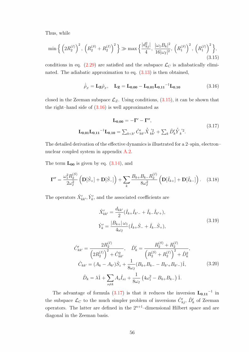
Thus, while

min{(

2R(I)2

)2

,(R

(S)2 +R

(I)2

)2 }� max

{ |d2kj|4,|ω1Bk|2

16|ωI |2,(R

(S)1

)2

,(R

(I)1

)2 },

(3.15)

conditions in eq. (2.29) are satisfied and the subspace LC is adiabatically elimi-

nated. The adiabatic approximation to eq. (3.13) is then obtained,

˙ρZ

= LZρZ , LZ = L0,00 − L0,01L0,11−1L0,10 (3.16)

closed in the Zeeman subspace LZ . Using conditions, (3.15), it can be shown that

the right–hand side of (3.16) is well approximated as

L0,00 = −Γ′ − Γ′′,

L0,01L0,11−1L0,10 =

∑k<k′ C

′kk′

ˆX′2kk′ +

∑k D

′k

ˆY′2k .

(3.17)

The detailed derivation of the effective dynamics is illustrated for a 2–spin, electron–

nuclear coupled system in appendix A.2.

The term L00 is given by eq. (3.14), and

Γ′′ =ω2

1R(S)2

2ω2I

(D[S+] + D[S−]

)+∑k

Bk+Bk−R(I)2

8ω2I

(D[Ik+] + D[Ik−]

). (3.18)

The operators X ′kk′ , Y′k , and the associated coefficients are

X ′kk′ =dkk′

2(Ik+Ik′− + Ik−Ik′+),

Y ′k =|Bk+|ω1

4ωI(Ik+S− + Ik−S+),

(3.19)

C ′kk′ =2R

(I)2(

2R(I)2

)2

+ C2kk′

, D′k =R

(S)2 +R

(I)2(

R(S)2 +R

(I)2

)2

+ D2k

,

Ckk′ = (Ak − Ak′)Sz +1

8ωI(Bk+Bk− −Bk′+Bk′−)1,

Dk = λ1 +∑s 6=k

AsIsz +1

8ωI

(4ω2

1 −Bk+Bk−)

1.

(3.20)

The advantage of formula (3.17) is that it reduces the inversion L0,11−1 in

the subspace LC to the much simpler problem of inversions C ′kj, D′k of Zeeman

operators. The latter are defined in the 2n+1–dimensional Hilbert space and are

diagonal in the Zeeman basis.

56

3.1.4 The Lindblad form

Utilizing the double–commutator, it is straightforward to re–write the right–hand

side of the Zeeman projected equation (3.16) in the purely Lindblad form, eq.

(2.11)

LZ = Γ(S)+ D(S+) + Γ

(S)− D(S−) +

∑k

Γ(I)k±

(D(Ik+) + D(Ik−)

)(3.21)

+∑k

Γ(IS)k D(Yk) +

∑k<k′

Γ(II)kk′ D(Xkk′).

The constant rates

Γ(S)± =

1∓ P0

2R

(S)1 +

ω21

2ω2I

R(S)2 , (3.22)

Γ(I)k± =

1

2

(R

(I)1 +

|Bk|2

4ω2I

R(I)2

), (3.23)

are related to the single–spin jump operators S±, Ik±, and the operator rates

Γ(IS)k =

ω21 |Bk+|2

8ω2I (R

(S)2 +R

(I)2 )

(1 + D2k)−1, (3.24)

Γ(II)kk′ =

d2kk′

4R(I)2

(1 + C2kk′)

−1, (3.25)

are related to the two–spin jump operators Xkk′ , and Yk;

Xkk′ = Ik+Ik′− + Ik−Ik′+,

Yk = Ik+S− + Ik−S+.

The re–written operator–valued coefficients Dk, Ckk′ are:

Dk =λ1 +

∑s 6=k AsIsz + 1

8ωI(4ω2

1 − |Bk+|2) 1

R(S)2 +R

(I)2

, (3.26)

Ckk′ =(Ak − Ak′)Sz + 1

8ωI(|Bk+|2 − |Bk′+|2)1

2R(I)2

. (3.27)

It is worth noting that for the operator–valued coefficient Ckk′ , eq. (3.27), the

second part, 18ωI

(|Bk+|2 − |Bk′+|2)1 is negligible in comparison to the first, hence

57

the rate Γ(II)kk′ is approximately state–independent, as

C2kk′ ≈

[(Ak − Ak′)Sz

]2

(2R(I)1 )2

=(Ak − Ak′)2

16 R(I)1

2 .

The situation is similar for eq. (3.26), where the term 18ωI

(4ω21 − |Bk+|2) is small in

comparison to the rest of terms, hence effectively eq. (3.26) can be approximated

to

Dk ≈λ1 +

∑s 6=k AsIsz

R(S)2 +R

(I)2

.

To implement the Zeeman–projected master equation, eq. (3.21), in the compu-

tationally convenient form of eq. (2.12), a correct treatment of the operator rates,

Ckk′ , Dk must be implemented. This procedure is described in appendix A.3.

3.1.5 Analysis of SE–DNP effective dynamics

The effective dynamics, outlined in eqs. (3.22 - 3.25) provide insight into the dy-

namics of SE–DNP, with much more clarity than the starting master equation,

eq. (3.2). The transfer of polarization from an electron to surrounding nuclei, po-

larization transport between nuclei and dissipative processes are all well described

by the four terms of the Lindbladian.

Electron relaxation

Equation (3.22) describes longitudinal relaxation of the central electron spin. This

is governed by spin–flips ’up’ (+) and ’down’ (-). The longitudinal relaxation rate

is weighted by the thermal electron polarization of the two states to ensure that

the electron relaxes back to thermal equilibrium. A comparison to eq. (3.1) shows

a perturbative, second order correction to the longitudinal relaxation of this spin.

This is a consequence of the applied microwave field; it relies on the microwave

field amplitude, ω1, the nuclear Larmor frequency ωI , and the electronic transverse

relaxation time R(S)2 . The driving microwave field effectively tilts the quantization

axis of the electron away from the Zeeman axis. The perturbative correction

corrects for this, approximating dynamics in a diagonal frame.

Nuclear relaxation

Equation (3.23) describes longitudinal relaxation of the nuclear spins. Since even

at low temperatures the thermal polarization of nuclear spins is very low, these

rates approximately coincide, and without any driving the nuclear spins will relax

to a state of no thermal polarization. A comparison to eq. (3.1) shows that

58

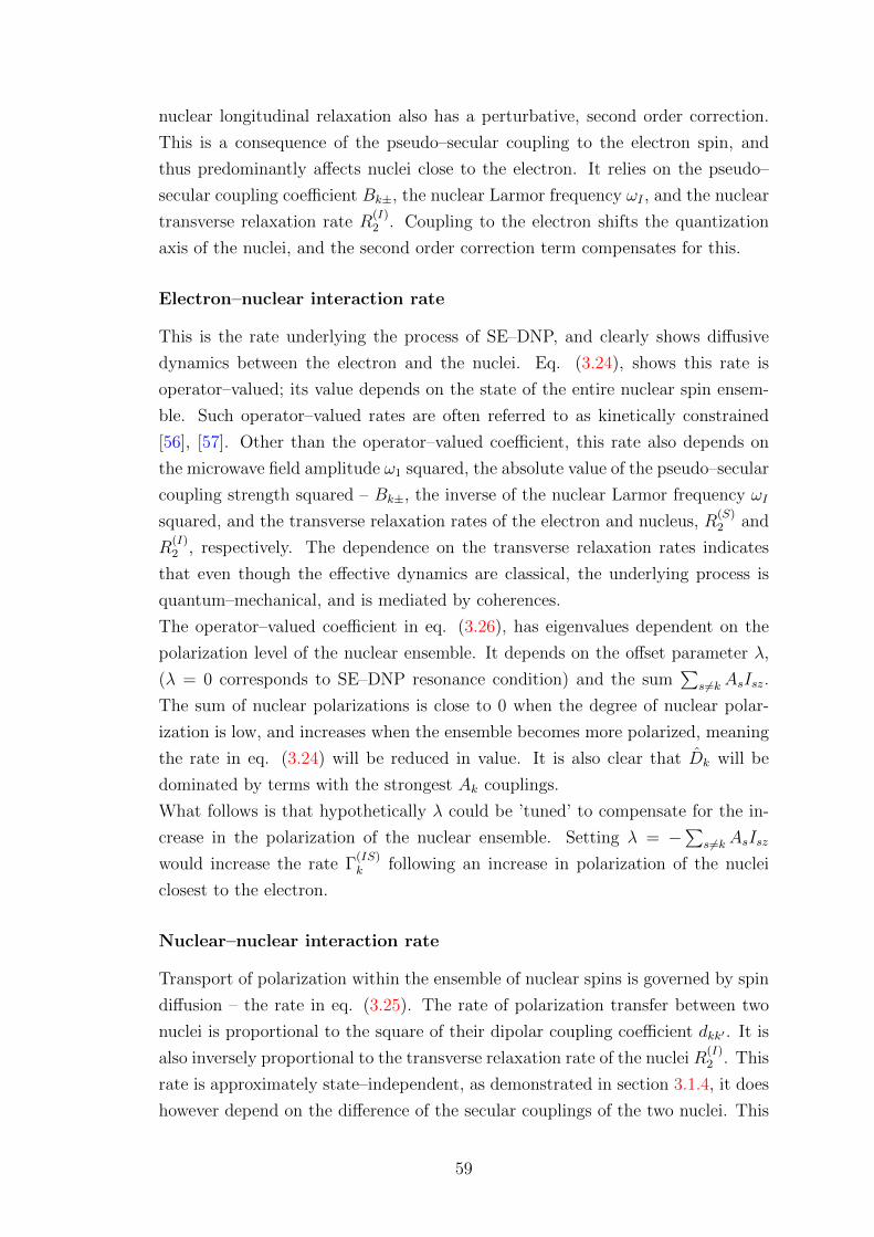
nuclear longitudinal relaxation also has a perturbative, second order correction.

This is a consequence of the pseudo–secular coupling to the electron spin, and

thus predominantly affects nuclei close to the electron. It relies on the pseudo–

secular coupling coefficient Bk±, the nuclear Larmor frequency ωI , and the nuclear

transverse relaxation rate R(I)2 . Coupling to the electron shifts the quantization

axis of the nuclei, and the second order correction term compensates for this.

Electron–nuclear interaction rate

This is the rate underlying the process of SE–DNP, and clearly shows diffusive

dynamics between the electron and the nuclei. Eq. (3.24), shows this rate is

operator–valued; its value depends on the state of the entire nuclear spin ensem-

ble. Such operator–valued rates are often referred to as kinetically constrained

[56], [57]. Other than the operator–valued coefficient, this rate also depends on

the microwave field amplitude ω1 squared, the absolute value of the pseudo–secular

coupling strength squared – Bk±, the inverse of the nuclear Larmor frequency ωI

squared, and the transverse relaxation rates of the electron and nucleus, R(S)2 and

R(I)2 , respectively. The dependence on the transverse relaxation rates indicates

that even though the effective dynamics are classical, the underlying process is

quantum–mechanical, and is mediated by coherences.

The operator–valued coefficient in eq. (3.26), has eigenvalues dependent on the

polarization level of the nuclear ensemble. It depends on the offset parameter λ,

(λ = 0 corresponds to SE–DNP resonance condition) and the sum∑

s 6=k AsIsz.

The sum of nuclear polarizations is close to 0 when the degree of nuclear polar-

ization is low, and increases when the ensemble becomes more polarized, meaning

the rate in eq. (3.24) will be reduced in value. It is also clear that Dk will be

dominated by terms with the strongest Ak couplings.

What follows is that hypothetically λ could be ’tuned’ to compensate for the in-

crease in the polarization of the nuclear ensemble. Setting λ = −∑

s 6=k AsIsz

would increase the rate Γ(IS)k following an increase in polarization of the nuclei

closest to the electron.

Nuclear–nuclear interaction rate

Transport of polarization within the ensemble of nuclear spins is governed by spin

diffusion – the rate in eq. (3.25). The rate of polarization transfer between two

nuclei is proportional to the square of their dipolar coupling coefficient dkk′ . It is

also inversely proportional to the transverse relaxation rate of the nuclei R(I)2 . This

rate is approximately state–independent, as demonstrated in section 3.1.4, it does

however depend on the difference of the secular couplings of the two nuclei. This

59

is a consequence of the coupling to the electron shifting the Larmor frequencies

of the nuclei. If the difference between the frequencies of the two nuclei becomes

significant, then the interaction between them becomes ineffective. In such case

the rate, eq. (3.25) becomes quenched and very little or no polarization transfer

takes place.

3.2 Error testing of Zeeman projection in SE–

DNP

The effective SE–DNP dynamics are an approximation to the dynamics in a diago-

nal frame. It is important to know when the assumptions underlying the projection

are valid. The conditions for the Zeeman projection are outlined in eq. (3.15).

For the rate Γ(IS)k , we require

1� |ω1||Bk|2

16(ωI)2(R(S)2 +R

(I)2 )2

.

For a hydrogen nucleus, in a modest magnetic field of BZ = 3.4 T, ωI = 144.8

MHz. Setting the transverse relaxation rates to: R(I)2 = 104 (s−1), R

(S)2 = 105

(s−1), the above condition is satisfied for example parameters of ω1 = 500 kHz,

Bk± = 30 MHz, giving

|ω1||Bk|2

16(ωI)2(R(S)2 +R

(I)2 )2

∼ 0.012� 1.

For the rate Γ(II)kk′ , we require

1� (dkk′)2

8(R(I)2 )2

Selecting again R(I)2 = 104, the above is satisfied for dkk′ on the order of a few

kilohertz. For dkk′ = 4 kHz,

(dkk′)2

8(R(I)2 )2

∼ 0.02� 1.

In order to verify the accuracy of the Zeeman projection more carefully, a more

systematic approach was taken. The virtual system pictured in fig. 3.1 was used

with variable separation a (for 2 A ≤ a ≤ 10 A). The nuclear coordinates are

given in table (3.1). Since the coupling strength between spins is not affected by

azimuthal rotations, most of the spins are placed in the y–z plane.

60

Figure 3.1: Test system, consisting of 5 nuclei (blue dots) surrounding an electron(red dot). The nuclear coordinates are given in the table below.

Spin x y z

S 0 0 0

I1 −a 0 0

I2 0 0 −aI3

a√2

0 a√2

I4a√2

0 a(1 +√22 )

I5 0 −a√32 −a

2

Table 3.1: Coordinate table.

Based on the separation a, the dipolar coupling strength dkk′ , secular coupling

Ak, and pseudo–secular coupling Bk± will vary accordingly. The simulations were

carried out using the gyromagnetic ratio of a 1H nucleus, and a magnetic field

of 3.4 T. In order to generate a significant nuclear polarization enhancement, it

was necessary to use a microwave field amplitude of 500 kHz for an inter–spin

separation of a = 2A. Such microwave field strength would be very difficult to

generate experimentally without a resonance cavity. The remaining simulation

parameters were: T = 1 K, T(S)1 = 1 ms, T

(I)1 = 1 h, T

(S)2 = 200 ns, T

(I)2 = 0.2

ms. The simulation duration (build–up time) was 1h. These parameters were

61

consistently used for a separations of 2–5 A.

The error testing was performed by comparing results obtained using the full

Liouvillian, eq. (3.2), and the Liouvillian projected into the Zeeman subspace –

eq. (3.21). In each case, the polarization curves of the nuclei are normalised to

the electronic thermal equilibrium polarization.

Figure 3.2: Nuclear polarization curves for a = 2A. The spins are numbered inthe legend in the same order as shown in table 3.1.

Figure 3.3: Error between full Liouvillian and Zeeman–projected master equationat a = 2A. A maximum error of 2.2 % is seen in the early stages of the simulation,and this falls to 1.5 % at steady–state.

62

Polarization curves for the system in fig. 3.1, when a = 2 A are shown in

figure 3.2. It can be seen that most of the nuclei in the system very quickly reach

steady–state. Nuclei with very weak pseudo–secular coupling (e.g. I1), take longer

to reach a steady–state, as would be expected. At approximately 800 s, all spins

are at steady–state.

Figure 3.3 shows a maximum error of approximately 2.2 % for a spin separation

of 2 A. This error falls below 1.5 % at steady–state. The error is seen to be lower

at larger spin–spin separations, as can be seen in figs. 3.4 – 3.7.

Figure 3.4: Error for a = 3 A (LHS) and 4 A (RHS). The error never exceeds 1%.

At separations of a = 3 A and 4 A the error is around 1 % in the very early

dynamics, and falls to 0.3 % and ∼ 0.1 % respectively, at steady state.

For separations of a = 5–10 A, the microwave field amplitude was reduced to an

experimentally more reallistic strength of 200 kHz, and the electronic transverse

relaxation time constant T(S)2 was increased 5–fold to T

(S)2 = 1 µs. For a = 5 A

there is an error of 0.15 % in the early dynamics, and this value falls as the system

approaches steady–state.

Figure 3.5: Error for a = 5 A (LHS) and 6 A (RHS).

63

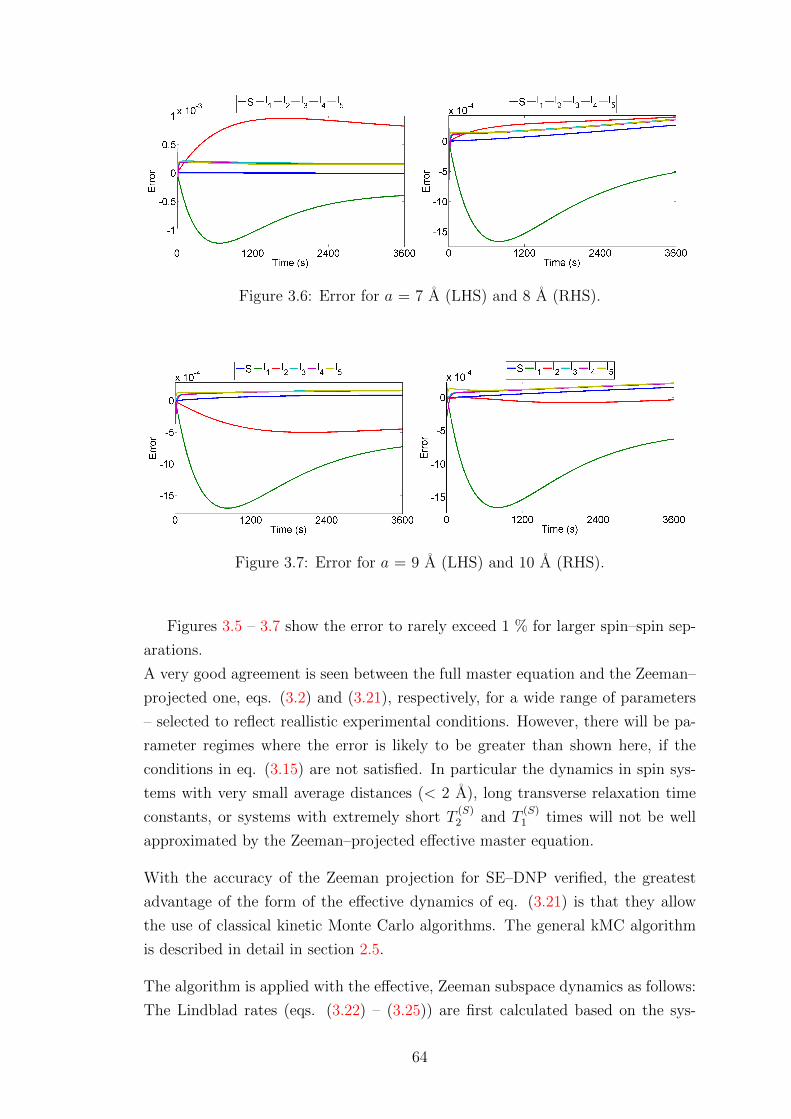
Figure 3.6: Error for a = 7 A (LHS) and 8 A (RHS).

Figure 3.7: Error for a = 9 A (LHS) and 10 A (RHS).

Figures 3.5 – 3.7 show the error to rarely exceed 1 % for larger spin–spin sep-

arations.

A very good agreement is seen between the full master equation and the Zeeman–

projected one, eqs. (3.2) and (3.21), respectively, for a wide range of parameters

– selected to reflect reallistic experimental conditions. However, there will be pa-

rameter regimes where the error is likely to be greater than shown here, if the

conditions in eq. (3.15) are not satisfied. In particular the dynamics in spin sys-

tems with very small average distances (< 2 A), long transverse relaxation time

constants, or systems with extremely short T(S)2 and T

(S)1 times will not be well

approximated by the Zeeman–projected effective master equation.

With the accuracy of the Zeeman projection for SE–DNP verified, the greatest

advantage of the form of the effective dynamics of eq. (3.21) is that they allow

the use of classical kinetic Monte Carlo algorithms. The general kMC algorithm

is described in detail in section 2.5.

The algorithm is applied with the effective, Zeeman subspace dynamics as follows:

The Lindblad rates (eqs. (3.22) – (3.25)) are first calculated based on the sys-

64

tem parameters. The rate for the flip–flop interaction between an electron and a

nucleus (eq. (3.24)) is state–dependent and hence is initiated using the thermal

equilibrium state. Next, two random numbers r1 and r2 are generated. The time

required for the next event to take place is calculated using a natural logarithm of

the first random number and the inverse of the sum of all rates of jumps that are

possible in the system. In the next step it is decided which type of jump will be

carried out. For this purpose all rates are normalised to sum up to 1, and arranged

in a cumulative sum array. An element in this array is identified which is higher in

value than the second random number. The operation corresponding to that rate

in the array element is then carried out. Accordingly, operations with higher rate

values are statistically more likely to occur than events with low rates. Once the

operation or jump is carried out, the effective rates for the flip flop jump between

a nucleus and the electron (eq. (3.24)) are re–calculated based on the current

system state. The steps outlined are repeated until a desired time is reached in

the trajectory. Many trajectories are computed and averaged to approximate the

polarization dynamics of the system. As previously discussed; the method does

not require vast amounts of memory since only an (n + 1)–element binary array

is required that stores the current orientation of the z–component (spin state) of

each individual spin.

Figure 3.8: Comparison of polarization curves computed using eq. (3.21) – solidblack lines, to the polarization curves approximated using kinetic Monte Carloalgorithms – dashed coloured lines. A good fit is seen between the two. Thepolarization curves estimated using kMC show an inherent random error that isreduced with averaging over a higher number of trajectories. The labelling ofnuclear spins corresponds to the labelling used in table 3.1.

65

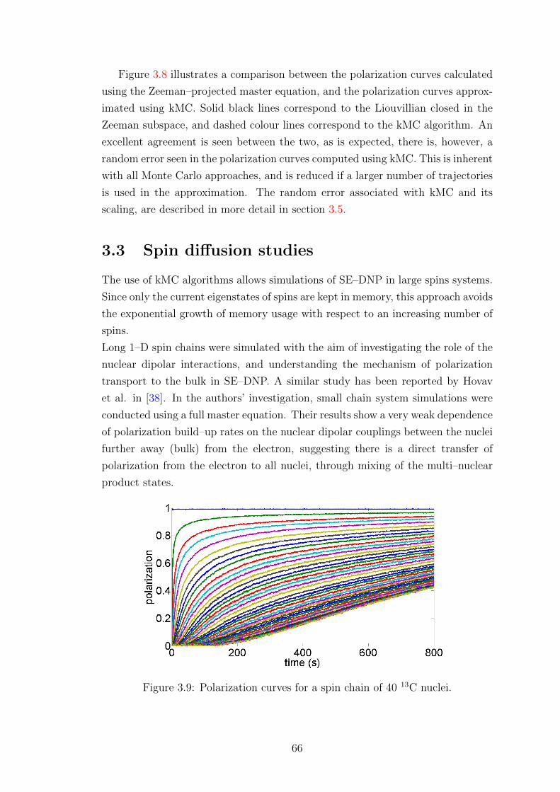
Figure 3.8 illustrates a comparison between the polarization curves calculated

using the Zeeman–projected master equation, and the polarization curves approx-

imated using kMC. Solid black lines correspond to the Liouvillian closed in the

Zeeman subspace, and dashed colour lines correspond to the kMC algorithm. An

excellent agreement is seen between the two, as is expected, there is, however, a

random error seen in the polarization curves computed using kMC. This is inherent

with all Monte Carlo approaches, and is reduced if a larger number of trajectories

is used in the approximation. The random error associated with kMC and its

scaling, are described in more detail in section 3.5.

3.3 Spin diffusion studies

The use of kMC algorithms allows simulations of SE–DNP in large spins systems.

Since only the current eigenstates of spins are kept in memory, this approach avoids

the exponential growth of memory usage with respect to an increasing number of

spins.

Long 1–D spin chains were simulated with the aim of investigating the role of the

nuclear dipolar interactions, and understanding the mechanism of polarization

transport to the bulk in SE–DNP. A similar study has been reported by Hovav

et al. in [38]. In the authors’ investigation, small chain system simulations were

conducted using a full master equation. Their results show a very weak dependence

of polarization build–up rates on the nuclear dipolar couplings between the nuclei

further away (bulk) from the electron, suggesting there is a direct transfer of

polarization from the electron to all nuclei, through mixing of the multi–nuclear

product states.

Figure 3.9: Polarization curves for a spin chain of 40 13C nuclei.

66

To explore this, simulations of 1–D 13C chains were implemented, with spin

chain lengths ranging from 30 – 50 nuclear spins. In each simulation the spin chain

was placed at an angle of 45◦ to the magnetic field vector, BZ .

Figure 3.9 illustrates the polarization build–up curves for each of the nuclear spins

in the chain. The parameters were chosen in accordance with parameters selected

by the authors in ref. [38]. There is a slight delay in time between the build–up

of each successive spin in the chain, indicating behaviour characteristic of spin–

diffusion.

Figure 3.10: The dependence of mean nuclear polarization on coupling parametersin the spin chain.

In figure 3.10 the polarization build–up trajectories shown in fig. 3.9 are av-

eraged, to give the mean nuclear polarization build–up in time – blue line. A

comparison is then made for a variety of coupling parameters. The nucleus clos-

est to the electron is referred to as the core nucleus, the remainder of nuclei are

treated as the bulk. The red line shows the difference in polarization build–up if

the nucleus–nucleus coupling parameter dkk′ for the bulk nuclei is halved. A large

drop in polarization is observed, and the polarization build–up rate is much slower.

The black line shows outcome if all of the nuclear dipolar coupling parameters dkk′

are halved. The difference between the red and black lines is small in comparison

to the difference betweem the blue and red lines. The green line shows the po-

larization build–up seen if in addition to halving dkk′ values, the pseudo–secular

coupling parameter Bk+ of the core nucleus is reduced by√

2. The difference

between the black and green lines is negligible.

It is thus clearly seen in fig. 3.10 that the rate of polarization transport across the

chain shows a large dependence on the dipolar coupling parameters. This further

strengthens the argument spin diffusion is the mechanism of polarization trans-

port to the bulk. This is in contrast to the conclusions drawn in [38], where the

67

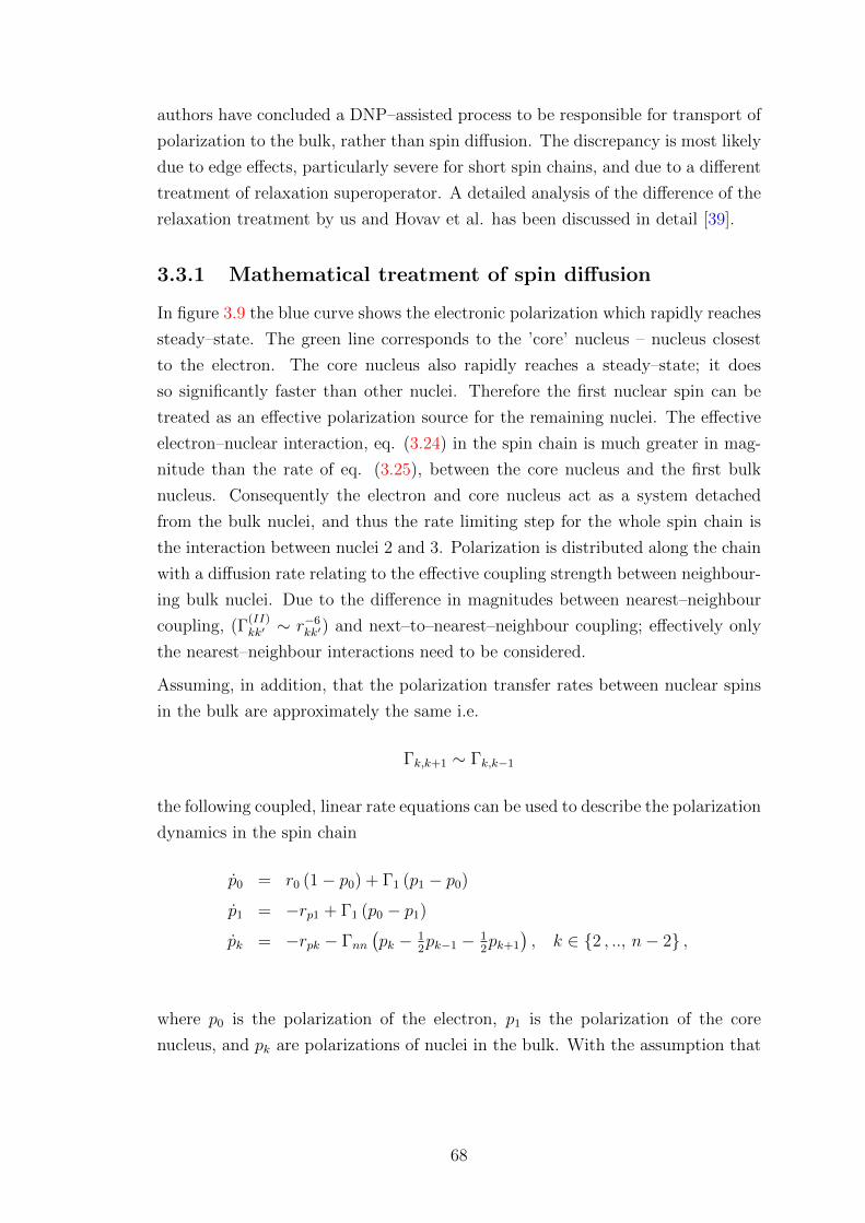
authors have concluded a DNP–assisted process to be responsible for transport of

polarization to the bulk, rather than spin diffusion. The discrepancy is most likely

due to edge effects, particularly severe for short spin chains, and due to a different

treatment of relaxation superoperator. A detailed analysis of the difference of the

relaxation treatment by us and Hovav et al. has been discussed in detail [39].

3.3.1 Mathematical treatment of spin diffusion

In figure 3.9 the blue curve shows the electronic polarization which rapidly reaches

steady–state. The green line corresponds to the ’core’ nucleus – nucleus closest

to the electron. The core nucleus also rapidly reaches a steady–state; it does

so significantly faster than other nuclei. Therefore the first nuclear spin can be

treated as an effective polarization source for the remaining nuclei. The effective

electron–nuclear interaction, eq. (3.24) in the spin chain is much greater in mag-

nitude than the rate of eq. (3.25), between the core nucleus and the first bulk

nucleus. Consequently the electron and core nucleus act as a system detached

from the bulk nuclei, and thus the rate limiting step for the whole spin chain is

the interaction between nuclei 2 and 3. Polarization is distributed along the chain

with a diffusion rate relating to the effective coupling strength between neighbour-

ing bulk nuclei. Due to the difference in magnitudes between nearest–neighbour

coupling, (Γ(II)kk′ ∼ r−6

kk′) and next–to–nearest–neighbour coupling; effectively only

the nearest–neighbour interactions need to be considered.

Assuming, in addition, that the polarization transfer rates between nuclear spins

in the bulk are approximately the same i.e.

Γk,k+1 ∼ Γk,k−1

the following coupled, linear rate equations can be used to describe the polarization

dynamics in the spin chain

p0 = r0 (1− p0) + Γ1 (p1 − p0)

p1 = −rp1 + Γ1 (p0 − p1)

pk = −rpk − Γnn(pk − 1

2pk−1 − 1

2pk+1

), k ∈ {2 , .., n− 2} ,

where p0 is the polarization of the electron, p1 is the polarization of the core

nucleus, and pk are polarizations of nuclei in the bulk. With the assumption that

68

rate of polarization transfer between bulk nuclei is constant along the chain;

pk = −rpk − Γnn (pk − pk−1) .

The nuclear polarization at thermal equilibrium is negligible, and generally in SE–

DNP Γ1 � Γnn, Γ1 � r0, Γnn � rp. It is therefore reasonable to assume in the

derivation that the polarization of the core nucleus is constant in time and close

in value to the electron quasi–steady–state polarization.

p1(t) ∼ 1 = const

The above assumptions work only if relaxation of nuclear spins in the system is

weak. Including dissipative contributions makes it difficult to solve the above

rate equations analytically. Neglecting edge effects and assuming the chain is

semi–infinite, in which case polarization is measured along a continuous spatial

coordinate ’x’, the equation describing polarization transfer from the core nucleus

to the rest of the nuclei can be written as

a2k

∂2p

∂x2≈ 1

2pk−1 + 1

2pk+1 − pk,

with ak being the effective separation between nuclei in the bulk. Since

∂p

∂t= Γnn(1

2pk−1 + 1

2pk+1 − pk),

the diffusion equation is recovered

∂p

∂t= D

∂2p

∂x2, (3.28)

where D = a2kΓnn. The solution to eq. (3.28) for the imposed initial conditions

pt=0,x>0 = 0, pt=0,x=0 ≈ = 1 is

p (x, t) = erfc

(x

2√Dt

), (3.29)

where erfc is the complimentary error function

erfc(x) =2√π

∫ ∞x

e−ε2

dε.

Setting eq. (3.29) equal to erfc(1), the diffusion length is obtained

x = 2√Dt. (3.30)

69

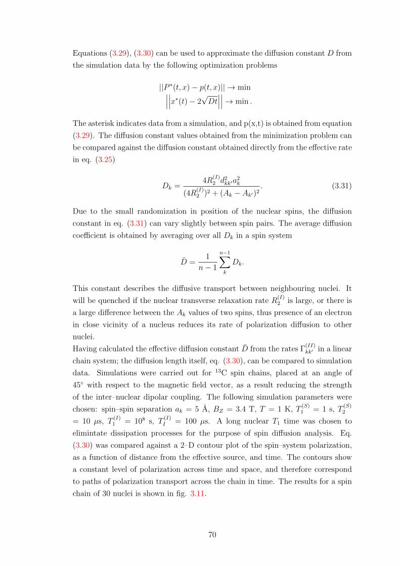
Equations (3.29), (3.30) can be used to approximate the diffusion constant D from

the simulation data by the following optimization problems

||P ∗(t, x)− p(t, x)|| → min∣∣∣∣∣∣x∗(t)− 2√Dt∣∣∣∣∣∣→ min .

The asterisk indicates data from a simulation, and p(x,t) is obtained from equation

(3.29). The diffusion constant values obtained from the minimization problem can

be compared against the diffusion constant obtained directly from the effective rate

in eq. (3.25)

Dk =4R

(I)2 d2

kk′a2k

(4R(I)2 )2 + (Ak − Ak′)2

. (3.31)

Due to the small randomization in position of the nuclear spins, the diffusion

constant in eq. (3.31) can vary slightly between spin pairs. The average diffusion

coefficient is obtained by averaging over all Dk in a spin system

D =1

n− 1

n−1∑k

Dk.

This constant describes the diffusive transport between neighbouring nuclei. It

will be quenched if the nuclear transverse relaxation rate R(I)2 is large, or there is

a large difference between the Ak values of two spins, thus presence of an electron

in close vicinity of a nucleus reduces its rate of polarization diffusion to other

nuclei.

Having calculated the effective diffusion constant D from the rates Γ(II)kk′ in a linear

chain system; the diffusion length itself, eq. (3.30), can be compared to simulation

data. Simulations were carried out for 13C spin chains, placed at an angle of

45◦ with respect to the magnetic field vector, as a result reducing the strength

of the inter–nuclear dipolar coupling. The following simulation parameters were

chosen: spin–spin separation ak = 5 A, BZ = 3.4 T, T = 1 K, T(S)1 = 1 s, T

(S)2

= 10 µs, T(I)1 = 108 s, T

(I)I = 100 µs. A long nuclear T1 time was chosen to

elimintate dissipation processes for the purpose of spin diffusion analysis. Eq.

(3.30) was compared against a 2–D contour plot of the spin–system polarization,

as a function of distance from the effective source, and time. The contours show

a constant level of polarization across time and space, and therefore correspond

to paths of polarization transport across the chain in time. The results for a spin

chain of 30 nuclei is shown in fig. 3.11.

70

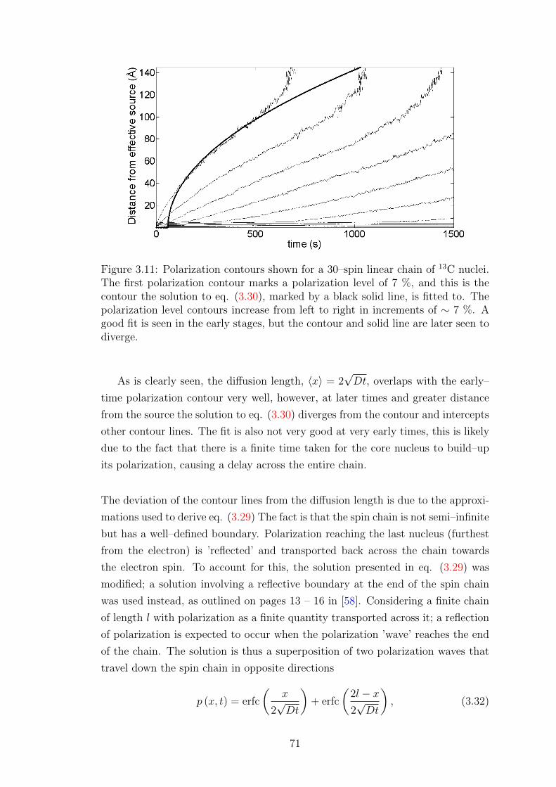
Figure 3.11: Polarization contours shown for a 30–spin linear chain of 13C nuclei.The first polarization contour marks a polarization level of 7 %, and this is thecontour the solution to eq. (3.30), marked by a black solid line, is fitted to. Thepolarization level contours increase from left to right in increments of ∼ 7 %. Agood fit is seen in the early stages, but the contour and solid line are later seen todiverge.

As is clearly seen, the diffusion length, 〈x〉 = 2√Dt, overlaps with the early–

time polarization contour very well, however, at later times and greater distance

from the source the solution to eq. (3.30) diverges from the contour and intercepts

other contour lines. The fit is also not very good at very early times, this is likely

due to the fact that there is a finite time taken for the core nucleus to build–up

its polarization, causing a delay across the entire chain.

The deviation of the contour lines from the diffusion length is due to the approxi-

mations used to derive eq. (3.29) The fact is that the spin chain is not semi–infinite

but has a well–defined boundary. Polarization reaching the last nucleus (furthest

from the electron) is ’reflected’ and transported back across the chain towards

the electron spin. To account for this, the solution presented in eq. (3.29) was

modified; a solution involving a reflective boundary at the end of the spin chain

was used instead, as outlined on pages 13 – 16 in [58]. Considering a finite chain

of length l with polarization as a finite quantity transported across it; a reflection

of polarization is expected to occur when the polarization ’wave’ reaches the end

of the chain. The solution is thus a superposition of two polarization waves that

travel down the spin chain in opposite directions

p (x, t) = erfc

(x

2√Dt

)+ erfc

(2l − x2√Dt

), (3.32)

71

and in such case the level curve corresponding to the diffusion length is found by

numerically solving

erfc

(x

2√Dt

)+ erfc

(2l − x2√Dt

)= erfc (1) , (3.33)

as there is no analytical solution.

The solution to eq. (3.33) is shown in comparison to eq. (3.30) for a spin chain

with 30 nuclei in figure 3.12. Other than at the very early stages of the dynamics,

the fit of reflective boundary solution (red line) to the polarization contour is very

good. The red line follows the contour shape much more closely than the black

line.

Figure 3.12: Polarization contours shown for a 30–spin linear chain of 13C nuclei.The first polarization contour marks a polarization level of 7 %, and the polar-ization level contours increase from left to right in increments of ∼ 7 %. Theblack line marks the solution to eq. (3.30). The reflective boundary solution, eq.(3.33), is shown in red. The reflective boundary solution matches the polarizationcontour much more closely, indicating that a semi–infinite chain treatment is notsuitable.

The same is seen for a slightly longer spin chain in fig. 3.13, where the spin

chain consists of 1 electron and 40 13C nuclear spins. Again, the red line, eq.

(3.33), matches the shape of the polarization contours much more closely.

72

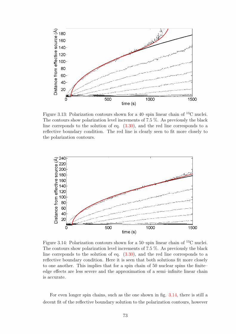
Figure 3.13: Polarization contours shown for a 40–spin linear chain of 13C nuclei.The contours show polarization level increments of 7.5 %. As previously the blackline correponds to the solution of eq. (3.30), and the red line corresponds to areflective boundary condition. The red line is clearly seen to fit more closely tothe polarization contours.

Figure 3.14: Polarization contours shown for a 50–spin linear chain of 13C nuclei.The contours show polarization level increments of 7.5 %. As previously the blackline correponds to the solution of eq. (3.30), and the red line corresponds to areflective boundary condition. Here it is seen that both solutions fit more closelyto one another. This implies that for a spin chain of 50 nuclear spins the finite–edge effects are less severe and the approximation of a semi–infinite linear chainis accurate.

For even longer spin chains, such as the one shown in fig. 3.14, there is still a

decent fit of the reflective boundary solution to the polarization contours, however

73

it can be seen that the fit is not as close as in fig. (3.12), for example. It is also

clear that the solutions to eqs. (3.30, 3.33) match each other much more closely,

thus indicating that the role of the reflective boundary becomes less important

for longer spin chains. The general fit being slightly worse than that seen in fig.

3.12 or fig. 3.9 is likely to be due to the randomization in spin position, leading

to a slight deviation of diffusion constant values across the chain from the average

diffusion coefficient value.

Our findings strongly suggest, therefore, that the transport of polarization to bulk

nuclei in SE–DNP is governed by spin diffusion. This work would not be possible

without the use of the effective dynamics and kMC. Moreover it is clear that small

spin–system simulations suffer quite severely from finite–boundary effects. This

signifies the advantage and necessity of using large–scale many body simulations

for understanding the physics of DNP.

3.4 Large spin ensemble calculations

The classical form of the equations governing the dynamics of SE–DNP, eqs. (3.22

– 3.25), enables efficient numerical treatment with the use of kinetic Monte Carlo

algorithms, in order to simulate and study large spin ensembles. The spin systems

in figures 3.11 – 3.14 are already far beyond the capability of the full master

equation, eq. (3.2), and therefore can already be considered large spin ensembles.

In this section, large spin system simulations of 3D cubic lattices are shown, to

demonstrate the capability of the effective treatment, and the insight it provides.

The parameters constant across all simulations are the temperature T = 1 K,

magnetic field strength, BZ = 3.4 T, and offset from the ZQ transition frequency

λ = 0.

3.4.1 Hydrogen nuclei

A 5x5x5 cubic lattice was simulated with a lattice constant of 30 A, making the

nearest–neighbour separation between nuclei 6 A. This value is close to the mean

proton–proton separation expected in DNP juice1. A 5 % uniform randomization

in the position of the spins was additionally applied to make the simulation more

realistic. A total of 124 1H nuclei surround the central electron spin. The following

relaxation times were chosen: T(S)1 = 1 s, T

(S)2 = 10 µs, T

(I)1 = 1 h, and T

(I)2 =

160/30/10 : d8–glycerol/D2O/H2O (vol %)

74

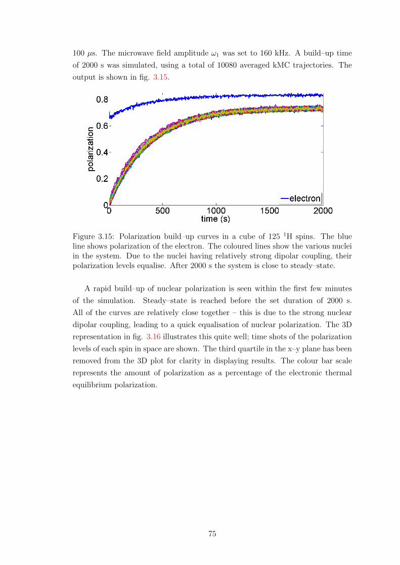
100 µs. The microwave field amplitude ω1 was set to 160 kHz. A build–up time

of 2000 s was simulated, using a total of 10080 averaged kMC trajectories. The

output is shown in fig. 3.15.

Figure 3.15: Polarization build–up curves in a cube of 125 1H spins. The blueline shows polarization of the electron. The coloured lines show the various nucleiin the system. Due to the nuclei having relatively strong dipolar coupling, theirpolarization levels equalise. After 2000 s the system is close to steady–state.

A rapid build–up of nuclear polarization is seen within the first few minutes

of the simulation. Steady–state is reached before the set duration of 2000 s.

All of the curves are relatively close together – this is due to the strong nuclear

dipolar coupling, leading to a quick equalisation of nuclear polarization. The 3D

representation in fig. 3.16 illustrates this quite well; time shots of the polarization

levels of each spin in space are shown. The third quartile in the x–y plane has been

removed from the 3D plot for clarity in displaying results. The colour bar scale

represents the amount of polarization as a percentage of the electronic thermal

equilibrium polarization.

75

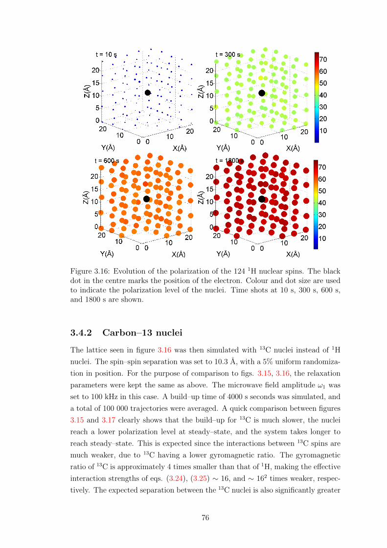
Figure 3.16: Evolution of the polarization of the 124 1H nuclear spins. The blackdot in the centre marks the position of the electron. Colour and dot size are usedto indicate the polarization level of the nuclei. Time shots at 10 s, 300 s, 600 s,and 1800 s are shown.

3.4.2 Carbon–13 nuclei

The lattice seen in figure 3.16 was then simulated with 13C nuclei instead of 1H

nuclei. The spin–spin separation was set to 10.3 A, with a 5% uniform randomiza-

tion in position. For the purpose of comparison to figs. 3.15, 3.16, the relaxation

parameters were kept the same as above. The microwave field amplitude ω1 was

set to 100 kHz in this case. A build–up time of 4000 s seconds was simulated, and

a total of 100 000 trajectories were averaged. A quick comparison between figures

3.15 and 3.17 clearly shows that the build–up for 13C is much slower, the nuclei

reach a lower polarization level at steady–state, and the system takes longer to

reach steady–state. This is expected since the interactions between 13C spins are

much weaker, due to 13C having a lower gyromagnetic ratio. The gyromagnetic

ratio of 13C is approximately 4 times smaller than that of 1H, making the effective

interaction strengths of eqs. (3.24), (3.25) ∼ 16, and ∼ 162 times weaker, respec-

tively. The expected separation between the 13C nuclei is also significantly greater

76

than that of 1H, weakening the effective dipolar interaction further by a factor of

∼ (10.3/6)6.

Figure 3.17: Polarization build–up curves for a cube of 125 13C nuclei. The blueline shows polarization of the electron. The coloured lines show the various nucleiin the system. In 13C, the dipolar coupling is weaker than in 1H, hence the nuclearpolarization levels do not equalise as well. After 4000 s the system is close tosteady–state.

The microwave field amplitude ω1 chosen to produce the simulation in fig.

3.15 was 60 % higher than that for fig. 3.17. This is due to the fact that the 1H

nuclei are coupled to the electron more effectively and depolarize the electron more

efficiently, thus the electron does not saturate. In figure 3.17 it is evident that the

electron polarization level is much lower, due to 13C coupling to the electron being

much weaker. The 13C nuclei do not depolarize the electron spin as efficiently,

hence it is closer to saturation by the the microwave field. A higher microwave

field amplitude ω1 would not be beneficial in this case. It is very likely it would

have a negative effect instead. The fact that the 13C–13C coupling is much weaker

manifests itself in fig. 3.17 – the polarization curves show a lot more spread than

those in fig. 3.15. This is also shown more clearly in the 3D figures, 3.18. The

plots clearly show that nuclei closer to the electron (with greatest Bk± values)

have a higher degree of polarization than nuclei at the edge of the lattice. It is

clear that the spin–diffusion rate is much slower for 13C nuclei.

77

Figure 3.18: Evolution of polarization of the 125 13C nuclear spins. The black dotin the centre marks the position of the electron. Colour and dot size are used toindicate the polarization level of the nuclei. Time shots at 10 s, 300 s, 600 s, and1800 s are shown, as a comparison against figure 3.16.

3.4.3 Carbon–13 – large spin system simulations

Following the simulations shown in figs. 3.15 – 3.18, cubic lattices with 73, 93, and

113 spins were simulated. Odd numbers were always chosen for the dimension size

in order to place the electron radical exactly in the centre of the lattice. For all

cases, the microwave field amplitude ω1 was ∼ 100 kHz. The following relaxation

parameters apply to all three cases: T(S)1 = 1 s, T

(S)2 = 10 µs, T

(I)2 = 100 µs.

The separation between nuclei was set to be ∼ 10 A; with 5 % randomization

in position. A build–up time of 4000 s was simulated in each case. For the spin

systems with 73, and 93; T(I)1 = 1 h. For the lattice with 113 nuclear spins,

T(I)1 = 1 h. Polarization dynamics were approximated by averaging over 100 000

trajectories, 20 000 trajectories, 10 000 trajectories for the spin systems with: 343

spins, 729 spins, and 1331 spins respectively.

78

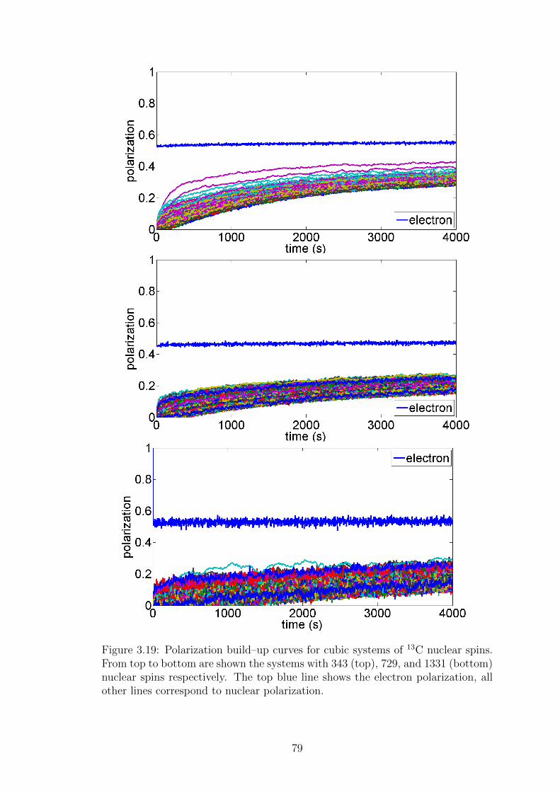
Figure 3.19: Polarization build–up curves for cubic systems of 13C nuclear spins.From top to bottom are shown the systems with 343 (top), 729, and 1331 (bottom)nuclear spins respectively. The top blue line shows the electron polarization, allother lines correspond to nuclear polarization.

79

The lower numbers of trajectories averaged was due to the long times2 needed

to simulate the latter cases. The results are shown in fig. 3.19.

Figure 3.19 makes it very apparent that for larger spin systems the build–up time

and the time taken to reach steady–state are significantly longer. It also appears

that the steady–state polarization values the nuclear spins reach are lower. Given

the conclusion from section 3.3.1, it is expected the last subplot of figure 3.19

suffers from edge effects the least, and corresponds most closely to the build–up

that would be expected in a realistic experimental set–up. The spread in nuclear

polarization values in fig. 3.19 is much greater than that seen for a smaller sys-

tem with similar parameters – figure 3.17. The limiting factor is clearly the weak

interaction between 13C nuclei, leading to an inefficient transport of polarization.

This figure illustrates the importance of using large–scale system simulations in

understanding the dynamics that govern DNP. The polarization dynamics seen in

figs. 3.15 – 3.19 would not be reflected in small spin systems – this applies partic-

ularly to the distribution of polarization among spins, the polarization build–up

rates, and the steady–state polarization values reached. All of these properties

are visibly affected by the number of spins interacting in the system, and seem

especially important in cases where the inter–nuclear interactions are relatively

weak due to large separations of spins, small gyromagnetic ratios, or both.

A close look at figure 3.20 shows that some nuclei further from the electron

have unusually high polarization values i.e. higher than their surrounding neigh-

bours. This phenomenon is purely down to the random noise in the system, and

is affected by the number of trajectories averaged to approximate the polarization

curves of each spin. It is clear then, when looking at this figure, that a larger num-

ber of trajectories would be beneficial for a more accurate solution. The amplitude

of the noise is very likely to be due to the weak interactions in the system. If there

are weak interactions present in the system, these are dominated by other interac-

tions which have a higher probability of occurring as an event. Consequently the

weak interactions are not sampled enough in the 10 000 trajectory course of the

simulation. This under–sampling causes a significant error for nuclei further from

the electron. This discovery suggests that the error magnitude approximation for

the kMC method may depend on the number of spins in the system. This was

investigated, and the results are described in the next section.

2for 1331 spins, the total simulation run–time was ∼ 26 days, on a dual processor 20–coreworkstation. The processors in use were Intel Xeon E5–2690 v2 3.00 GHz.

80

Figure 3.20: Time–shots showing polarization of nuclear spins arranged in a cu-bic, regular lattice (11 × 11 × 11). The black dot in the centre is the electron.Polarization build–up is fastest for nuclei that are close to the electron and atan angle of π/4 with respect to BZ . The contribution of spin–diffusion is shownin the bottom figure. The bottom–right figure shows a system with no nucleardipolar interactions in comparison to the normal case in the bottom–left. Spinswithin one quarter of the cube are hidden for better visibility. The inserts showpolarization of nuclei in the planes marked in the top–left part of the figure.

The bottom part of figure 3.20 shows the importance of dipolar interactions,

and spin diffusion in the system. A simulation was carried out for a system without

any nuclear dipole interactions. On the RHS part of this figure, nuclei close to the

electron reach much greater levels of polarization, but there is no transport to the

bulk. In the LHS, the same core electrons are at a lower polarization level due to

transport of polarization to the bulk.

3.4.4 Fitting of polarization curves

The polarization build–up curves of individual nuclei are subject to random error.

Other than increasing the number of trajectories to average over in the kMC

simulations, the random error can be reduced by fitting the polarization curves

81

to an analytical function. This section describes the fitting approaching that has

been implemented – with some success. A suitable function for modelling the

build–up of polarization is

p(t) = pss(1− e−t/τ ),

where τ is the polarization build–up time constant, and pss is the polarization

reached at steady–state (t → ∞). Another possibility is to use a bi–exponential

fit of the form

p(t) = pss(1− e−t/τ1) + p′ss(1− e−t/τ2).

This fit now has two time–constants τ1, τ2, and each corresponds to a different

process contributing to build–up of polarization of a particular spin. Most likely,

in the case of the systems studied, this would include contributions of polarization

due to spin–diffusion, and direct contributions from the electron – applicable to

nuclei close to the electron. Polarization curves of nuclei further away from the

electron should fit a mono–exponential function quite well. A comparison to the

output of figure 3.17 is shown first, in figure 3.21. The bi–exponential function

was used for fitting in this case.

Figure 3.21: Polarization curves fitted to the output of figure 3.17 – a bi–exponential fit is used. On the right the fitting error, found by taking an absolutedifference between the two figures. This was done to clearly illustrate the max-imum error. Other than at the very early time of the simulation, the RHS plotshows the random error associated with kMC algorithms.

Other than at very early times of the simulation, the fit is very accurate, and

the error rarely exceeds 2 %. The adjusted R2 value rarely falls below 0.995.

Next, the fits to the polarization curves in figure 3.19 are shown.

82

Figure 3.22: Polarization curves fitted to the output of figure 3.19, and on the right,the fitting error, found by taking an absolute difference between the figures. Theabsolute value is taken for clarity to illustrate maximum error. With increasingspin system the random error clearly increases, as well as the error in the veryearly stages of the simulation.

The top figure corresponds to the simulation of the spin system with 343 spins.

The fit to the polarization curves is overall very good, with an adjusted R2 value

averaging at 0.995, and the error rarely exceeding 3 %. The middle part of fig-

ure 3.22 corresponds to the spin lattice with 729 nuclei. The fit is rather bad at

the very early stages of the simulation with the error reaching 10 %. This error

does, however, fall rapidly in time and stays below 4 % for the most part of the

polarization build–up. The adjusted R2 value averages at 0.97, indicating a good

quality fit overall. Considering, 20 000 trajectories were used for this simulation in

comparison to 100 000 in fig. 3.21, and the top part of fig. 3.22, this is a good fit.

It could be used for extrapolation to determine steady–state polarization values

of each spin.

The fit is much worse for the bottom part of fig. 3.22, where only 10 000 tra-

jectories have been averaged. The adjusted R2 value averages around 87 % for

83

the spins. As was the case in figures 3.21 and 3.22 (middle and top), the error is

larger in the early stages of polarization build–up, and then falls at later times.

Typically, the error stays at a maximum of around 6 % for some of the the spins.

Fitting to a higher number of terms

The figures showing a poorer fit, i.e. the middle and bottom parts of fig. 3.22

were then fitted to a function consisting of four exponential terms:

p(t) = pss(1− e−t/τ1) + p′ss(1− e−t/τ2) + p′′ss(1− e−t/τ3) + p′′′ss(1− e−t/τ4).

Whereas it is difficult to explain the presence of four different processes, each

acting over a different time–scale, the use of a quad–exponential fitting function

significantly improves the fit quality to the polarization build–up curves of the

spin system of 728 nuclei, as shown in fig. 3.23 below.

Figure 3.23: Fitting of the polarization curves from figure 3.19 (middle part), andassociated error. The fit is made using a function containing four exponentialterms. An absolute value of the error is taken. A much closer fit is found than infigure 3.22.

The fitting to a higher number of terms removes the error previously seen in

the early times of polarization build–up. The error due to the fitting does not

exceed 3.5 %, which is on the scale of random error expected from using kMC

algorithms.

In the case of the 1331–spin simulation, a fit with four terms reduces the large

error seen in the early stages of the simulation. The error during the rest of the

polarization build–up is not affected significantly.

84

Figure 3.24: Fitting of the polarization curves from figure 3.19 (bottom part),and associated error. The fit is made to a function containing four exponentialterms, and again an absolute value of the error is taken. A comparison to figure3.22 shows the early–stage error is reduced and thus a much better fit is found,with only the random error remaining. An increase in the maximum kMC randomerror is seen for larger spin systems.

It can be seen that the error is in the vicinity of 6 % for some nuclei. The mean

error (averaged over spins) is approximately 1.4 %. The fit can be considered quite

accurate, with the deviation from the lines of best fit being due to the random

error, which is inherent in all Monte Carlo algorithms. The fitting described in

this section can thus be effectively used to remove the random error of simulations

relying on the kMC algorithm.

A more comprehensive error analysis is described in the next section.

3.5 Monte Carlo scaling and error analysis

In this section the error associated with kMC algorithms is analysed more care-

fully. The scaling of the random error with respect to an increasing number of

trajectories is verified. The scaling of the error with respect to an increasing num-

ber of spins in the system is then shown. In the last part of this section, the

scaling of simulation duration is shown with respect to an increasing system size.

3.5.1 Scaling of error with number of spins

The analysis was mostly carried out using results from three simulations, carried

out for cubic systems containing 13C nuclei, with a uniform spin–spin separation

– subject a to a small degree of uniform randomization in spin position. The

same parameters were used in each simulation; BZ = 3.4 T, T = 1 K, T(S)1 = 1

s, T(S)2 = 10 µs, T

(I)1 = 1 h, T

(I)2 = 100 µs, spin–spin separation = 10.3 A. The

cubic lattices contained 3×3×3, 5×5×5, and 7×7×7 spins respectively. A 20 000

85

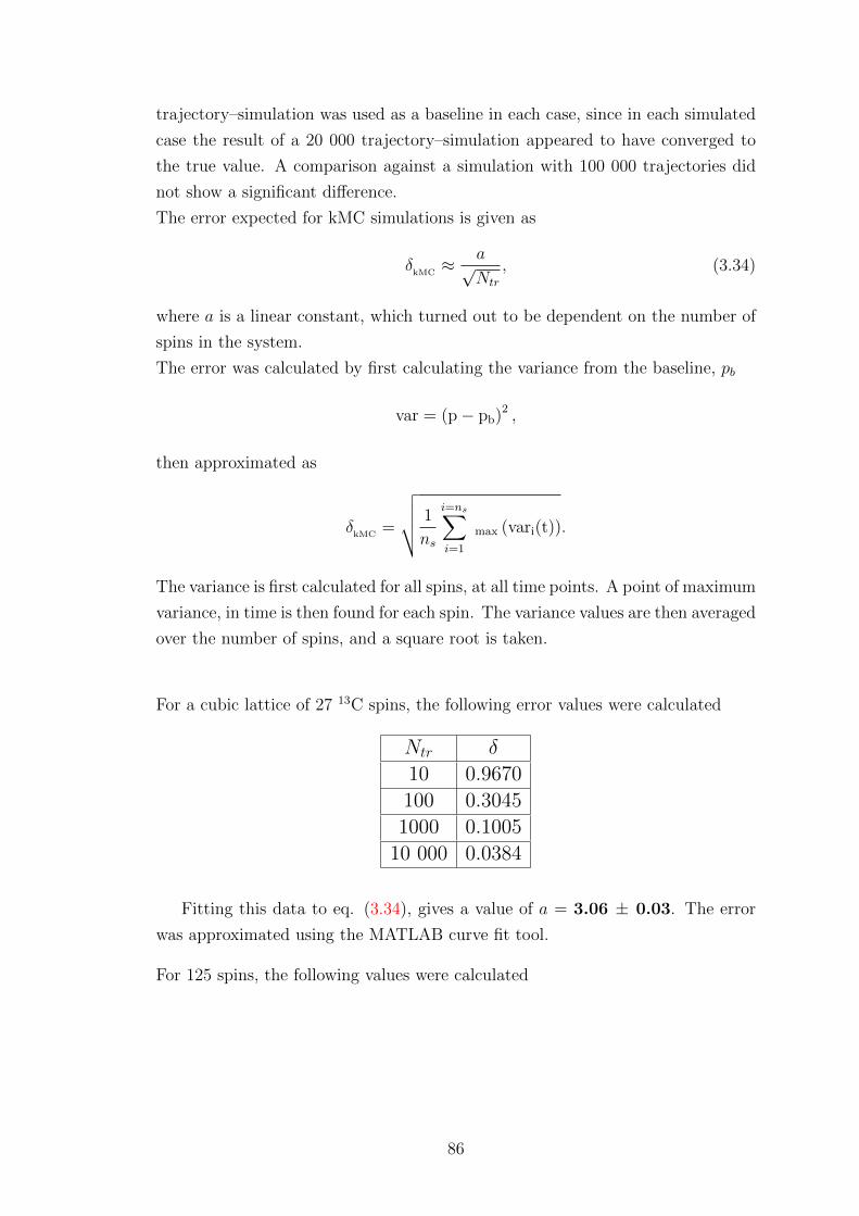
trajectory–simulation was used as a baseline in each case, since in each simulated

case the result of a 20 000 trajectory–simulation appeared to have converged to

the true value. A comparison against a simulation with 100 000 trajectories did

not show a significant difference.

The error expected for kMC simulations is given as

δkMC≈ a√

Ntr

, (3.34)

where a is a linear constant, which turned out to be dependent on the number of

spins in the system.

The error was calculated by first calculating the variance from the baseline, pb

var = (p− pb)2 ,

then approximated as

δkMC

=

√√√√ 1

ns

i=ns∑i=1

max (vari(t)).

The variance is first calculated for all spins, at all time points. A point of maximum

variance, in time is then found for each spin. The variance values are then averaged

over the number of spins, and a square root is taken.

For a cubic lattice of 27 13C spins, the following error values were calculated

Ntr δ

10 0.9670

100 0.3045

1000 0.1005

10 000 0.0384

Fitting this data to eq. (3.34), gives a value of a = 3.06 ± 0.03. The error

was approximated using the MATLAB curve fit tool.

For 125 spins, the following values were calculated

86

Ntr δ

10 1.0359

100 0.3348

1000 0.1085

10 000 0.0419

giving a value of a = 3.29 ± 0.03.

Finally, for 343 spins, the following values were calculated

Ntr δ

10 1.2105

100 0.5060

1000 0.1344

10 000 0.0538

Fitting this data to eq. (3.34), gives a value of a = 3.9 ± 0.3. It is also worth

noting that the error approximated this way is likely to be exaggerated. Figure

3.25 illustrates the value of a coefficients as a function of the number of spins in

the system, for the three cubic lattices.

Figure 3.25: Coefficient a from eq. 3.34 shown as a function of the number ofspins. It is seen here that with an increasing number of spins in the system, theerror associated with the kMC algorithm will also increase. The data here fits asecond order polynomial equation, indicating a quadratic scaling of the error withrespect to the number of spins.

The relationship of error as a function of the number of spins fits a quadratic

polynomial perfectly – with SSE = 0, and R2 = 1.

87

A simple extrapolation of the fit for a cubic lattice with 729 spins would suggest

a should be around ∼ 5. The value of a in the actual simulation results seemed

to decrease instead. This was investigated. For each simulation, histograms were

plotted showing the distribution of error values for different numbers of trajectories

averaged. First the histograms for the 27–spin simulation were plotted for varying

numbers of trajectories – 20 bins were used for histogram plotting.

Figure 3.26: Distribution of errors for a cubic lattice of 27 spins. From left to right;100 trajectories, 1000 trajectories, 10 000 trajectories were used respectively.

Next, the histograms for the 125 spin simulation were plotted (30 bins used

for histograms):

Figure 3.27: Distribution of errors for a cubic lattice of 125 spins. From left toright; 100 trajectories, 1000 trajectories, 10 000 trajectories.

Followed by the histograms for the 343 spin simulation (30 bins used for his-

tograms).

88

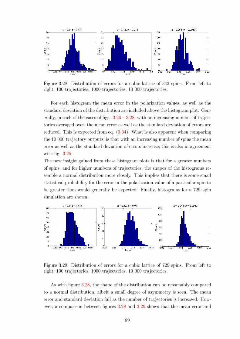
Figure 3.28: Distribution of errors for a cubic lattice of 343 spins. From left toright; 100 trajectories, 1000 trajectories, 10 000 trajectories.

For each histogram the mean error in the polarization values, as well as the

standard deviation of the distribution are included above the histogram plot. Gen-

erally, in each of the cases of figs. 3.26 – 3.28, with an increasing number of trajec-

tories averaged over, the mean error as well as the standard deviation of errors are

reduced. This is expected from eq. (3.34). What is also apparent when comparing

the 10 000 trajectory outputs, is that with an increasing number of spins the mean

error as well as the standard deviation of errors increase; this is also in agreement

with fig. 3.25.

The new insight gained from these histogram plots is that for a greater numbers

of spins, and for higher numbers of trajectories, the shapes of the histograms re-

semble a normal distribution more closely. This implies that there is some small

statistical probability for the error in the polarization value of a particular spin to

be greater than would generally be expected. Finally, histograms for a 729–spin

simulation are shown.

Figure 3.29: Distribution of errors for a cubic lattice of 729 spins. From left toright; 100 trajectories, 1000 trajectories, 10 000 trajectories.

As with figure 3.28, the shape of the distribution can be reasonably compared

to a normal distribution, albeit a small degree of asymmetry is seen. The mean

error and standard deviation fall as the number of trajectories is increased. How-

ever, a comparison between figures 3.28 and 3.29 shows that the mean error and

89

distribution of errors are generally lower for the 729–spin simulation. It is ex-

pected that the middle and RHS plots of fig. 3.29 are closer to the baseline than

the corresponding case in fig. 3.28. Rather than the solutions for the 729 spin

lattice being more accurate, they fit closer to a baseline, which in this case is

further away from the correct solution. In the case of this spins system, a solution

with more averaged trajectories would have to be used as a baseline.

It is expected that for simulations with even greater spin numbers, such as the

simulation with 1331 spins in fig. 3.20, a number of spins will have an error greater

than generally anticipated (3.5 %) for 10 000 averaged trajectories – as seen for

example in fig. 3.8. This also explains the error seen in some of the polarization

curves. The probability of the error being greater than this value is small (regions

far from the mean of the Gaussian), hence the number of spins with a large error

is expected to be small.

The nature of the random error associated with the Monte Carlo algorithms relies

on choosing an optimal number of trajectories to be averaged. If the number is

too small, the accuracy of the solution will be insufficient, on the other hand, too

large a number of trajectories is a waste of computational time. In accordance

with eq. (3.34) increasing the number of trajectories by ten–fold will increase the

simulation run–time by a factor of 10, but the error will only be reduced by a

factor of√

10.

If one is only interested in the mean ensemble polarization of a system, then a

lower number of trajectories can be used. The random nature of the errors means

that ensemble averaging of the polarization of spins will lead to averaging out of

the individual errors.

3.5.2 Scaling of simulation duration

As mentioned in section 2.5 – describing implementation of the kMC algorithm,

use of this algorithm circumvents the exponential scaling of memory usage with

respect to the number of spins. When using the kMC algorithm only the current

state of the system, coupling parameters, and effective rates are kept in memory.

The state of the system, as well as rates in eq. (3.23), (3.24) all scale linearly

with respect to an increasing number of spins. The rate in eq. (3.25) scales

quadratically with respect to an increasing number of spins. Thus, the memory

scaling with respect to an increasing number of spins is described by a second–

order polynomial. The CPU usage with an increasing number of spins is more

tricky to determine. This was analysed by measuring the time taken for 10 000

trajectories in simulations of systems depicted in figs. 3.18 and 3.19. The result

is shown below in figure 3.30.

90

Figure 3.30: Time taken for simulaions of spin systems with an increasing numberof spins. The point of 0 spins would naturally take no time. The times for thecubic 13C spin lattices are as follows: 125 spins – 0.5 h, 343 spins – 4.43 h, 729spins – 100 h, 1331 spins, 626 hours. The points fit a third order polynomial. Thesimulation duration also depends on the dipolar coupling parameter strengths,thus varying the spacing between the spins will also vary the computational time.

The line of best fit follows a third–order polynomial equation, with no offset

f(ns) = b(ns)3 + c(ns)

2 + d(ns),

very closely. The terms b, c, d are constant coefficients with values of b = 2.51×10−7

(± 31 %), c = 3.85×10−5 (± 100 %),d = -2.5×10−2 (± 100 %). It is clear then

that for larger spin systems (eg. 13×13×13), the time such a simulation would

take makes it unfeasible without the use of a supercomputer cluster.

3.6 Adiabatic elimination of Solid Effect dynam-

ics for hetero–nuclear spins

The adiabatic elimination projection of the SE–DNP dynamics onto the Zeeman

subspace can be carried out for a system consisting of hetero–nuclear spins, pro-

vided these are relatively close in frequency. One such example is a system con-

sisting of protons and fluorine nuclei. The projection is carried out in a similar

manner to that described in section 3.1. An offset from the SE–DNP resonances

for the nuclear spins is introduced - δ. For example, if the projection was to be

carried out for protons, all the 1H nuclei would have δ = 0, and the second species

91

(e.g. fluorine) will have an offset of δ = 1HωI − 19FωI .

For the zero–quantum subspace projection the strict mathematical requirement is

that 1Hδ � ωI . Formally the condition for this projection is then

ωI � Ak, Bk±, dkk′ , δk,Γ(S)z ,Γ

(S)± ,Γ

(I)kz ,Γ

(I)k±. (3.35)

The relaxation superoperator is unaltered. The system Hamiltonian becomes

HZ = ∆Sz +∑k

Ikz

H0 = λSz +∑k

δkIkz +∑k

AkSz Ikz +ω1

2(S+ + S−)

+dkk′∑kk′

(2Ikz Ik′z −1

2Ik+Ik′− −

1

2Ik−Ik′+)

H± =∑k

Bk±Sz Ik±.

The projection onto the Zeeman subspace is carried out exactly as before; subject

to the same conditions as described in eq. (3.15).

The effective dynamics are written in the Lindblad form, shown in eq. (2.11)

LZ = Γ(S)+ D(S+) + Γ

(S)− D(S−) +

∑k

Γ(I)k±

(D(Ik+) + D(Ik−)

). . . (3.36)

+∑k

Γ(IS)k D(Yk) +

∑k<k′

Γ(II)kk′ D(Xkk′).

The constant rates

Γ(S)± =

1∓ P0

2R

(S)1 +

ω21

2ω2I

R(S)2 , (3.37)

Γ(I)k± =

1

2

(R

(I)1 +

|Bk|2

4ω2I

R(I)2

), (3.38)

are related to the single–spin jump operators S±, Ik±. These are identical to the

homo–nuclear case, eqs. (3.22), (3.23). The operator rates

Γ(IS)k =

ω21 |Bk+|2

8ω2I (R

(S)2 +R

(I)2 )

(1 + D2k)−1, (3.39)

Γ(II)kk′ =

d2kk′

4R(I)2

(1 + C2kk′)

−1, (3.40)

92

are related to the two–spin jump operators Xkk′ , and Yk;

Xkk′ = Ik+Ik′− + Ik−Ik′+,

Yk = Ik+S− + Ik−S+.

The operator–values coefficients Dk, Ckk′ appearing in the above equations are:

Dk =(λ− δk)1 +

∑s 6=k AsIsz + 1

8ωI(4ω2

1 − |Bk+|2) 1

R(S)2 +R

(I)2

, (3.41)

Ckk′ =(δk − δk′)1 + (Ak − Ak′)Sz + 1

8ωI(|Bk+|2 − |Bk′+|2)1

2R(I)2

. (3.42)

It is worth noting that for the operator–valued coefficient Ckk′ , eq. (3.42), the last

part, 18ωI

(|Bk+|2 − |Bk′+|2 1 is as previously negligible in comparison to the first

two terms

C2kk′ ≈

[(δk − δk′) + (Ak − Ak′)Sz

]2

(2R(I)1 )2

.

3.6.1 Analysis of hetero–nuclear SE–DNP effective dynam-

ics

Electron–nuclear interaction rate

The addition of an offset parameter δk in the state–dependent coefficient Dk, in eq.

(3.41), means this coefficient will typically be large for large δk. For a magnetic

field of 3.4 T, and at the proton resonance; the δk for fluorine nuclei is ∼ 8.5 MHz.

This value would likely dominate the terms in eq. (3.41) and cause the rate Γ(IS)k

to be quenched for fluorine nuclei.

Nuclear–nuclear interaction rate

The form of the rate Γ(II)kk′ for a heteronuclear system depends on the difference

between the offsets δk in the coefficient Ckk′ – eq. (3.42) – of any two nuclei. This

implies that the effective internuclear interaction is efficient between spins of the

same species, but becomes inefficient between spins of different nuclei.

On the other hand, there exists a possibility for the offset difference δk − δkk′ to

cancel with Ak − Ak′ , or at least collectively reduce the magnitude of Ckk′ . Thus

cross–polarization under DNP for hetero–nuclear systems appears to be feasible,

even for the simplest of DNP mechanisms; SE–DNP.

93

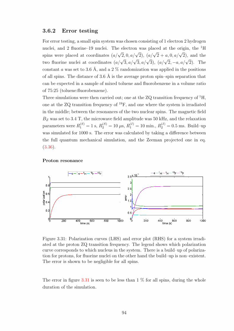
3.6.2 Error testing

For error testing, a small spin system was chosen consisting of 1 electron 2 hydrogen

nuclei, and 2 fluorine–19 nuclei. The electron was placed at the origin, the 1H

spins were placed at coordinates (a/√

2, 0, a/√

2), (a/√

2 + a, 0, a/√

2), and the

two fluorine nuclei at coordinates (a/√

3, a/√

3, a/√

3), (a/√

2,−a, a/√

2). The

constant a was set to 3.6 A, and a 2 % randomization was applied in the positions

of all spins. The distance of 3.6 A is the average proton spin–spin separation that

can be expected in a sample of mixed toluene and fluorobenzene in a volume ratio

of 75:25 (toluene:fluorobenzene).

Three simulations were then carried out; one at the ZQ transition frequency of 1H,

one at the ZQ transition frequency of 19F, and one where the system is irradiated

in the middle; between the resonances of the two nuclear spins. The magnetic field

BZ was set to 3.4 T, the microwave field amplitude was 50 kHz, and the relaxation

parameters were R(S)1 = 1 s, R

(S)2 = 10 µs, R

(I)1 = 10 min., R

(I)2 = 0.5 ms. Build–up

was simulated for 1000 s. The error was calculated by taking a difference between

the full quantum mechanical simulation, and the Zeeman projected one in eq.

(3.36).

Proton resonance

Figure 3.31: Polarization curves (LHS) and error plot (RHS) for a system irradi-ated at the proton ZQ transition frequency. The legend shows which polarizationcurve corresponds to which nucleus in the system. There is a build–up of polariza-tion for protons, for fluorine nuclei on the other hand the build–up is non–existent.The error is shown to be negligible for all spins.

The error in figure 3.31 is seen to be less than 1 % for all spins, during the whole

duration of the simulation.

94

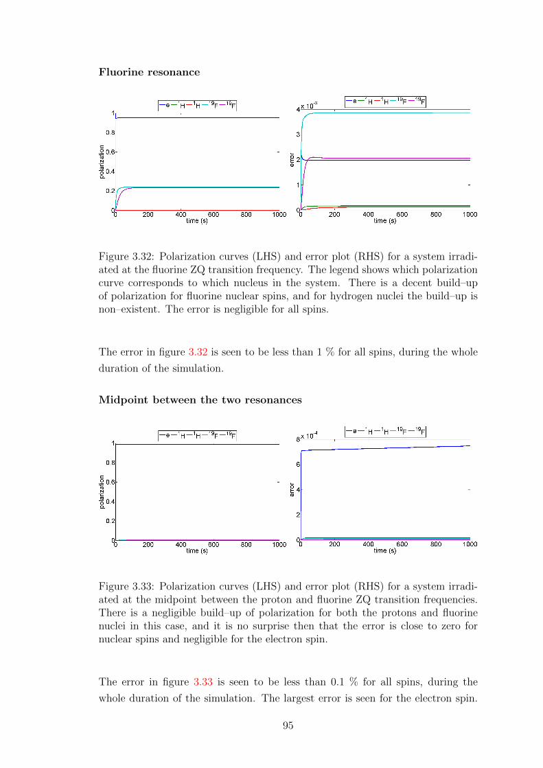
Fluorine resonance

Figure 3.32: Polarization curves (LHS) and error plot (RHS) for a system irradi-ated at the fluorine ZQ transition frequency. The legend shows which polarizationcurve corresponds to which nucleus in the system. There is a decent build–upof polarization for fluorine nuclear spins, and for hydrogen nuclei the build–up isnon–existent. The error is negligible for all spins.

The error in figure 3.32 is seen to be less than 1 % for all spins, during the whole

duration of the simulation.

Midpoint between the two resonances

Figure 3.33: Polarization curves (LHS) and error plot (RHS) for a system irradi-ated at the midpoint between the proton and fluorine ZQ transition frequencies.There is a negligible build–up of polarization for both the protons and fluorinenuclei in this case, and it is no surprise then that the error is close to zero fornuclear spins and negligible for the electron spin.

The error in figure 3.33 is seen to be less than 0.1 % for all spins, during the

whole duration of the simulation. The largest error is seen for the electron spin.

95

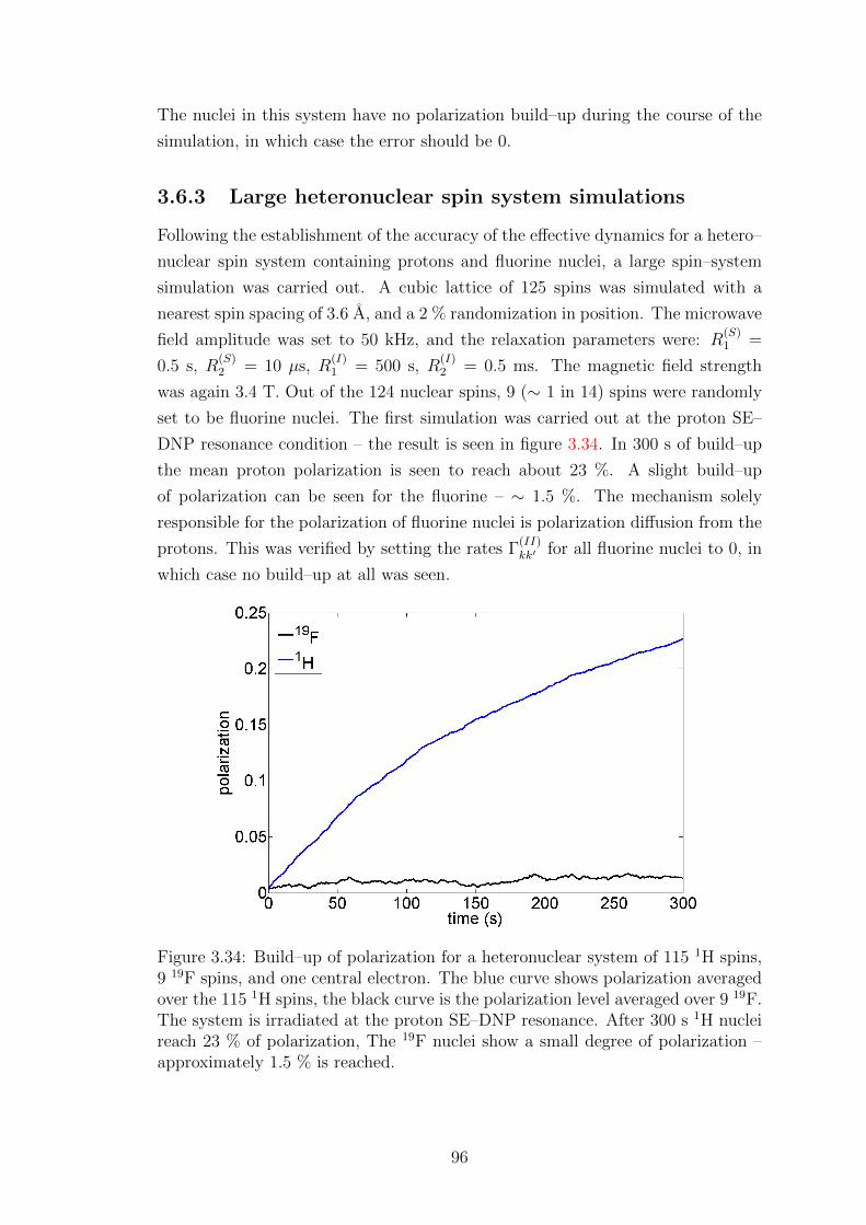
The nuclei in this system have no polarization build–up during the course of the

simulation, in which case the error should be 0.

3.6.3 Large heteronuclear spin system simulations

Following the establishment of the accuracy of the effective dynamics for a hetero–

nuclear spin system containing protons and fluorine nuclei, a large spin–system

simulation was carried out. A cubic lattice of 125 spins was simulated with a

nearest spin spacing of 3.6 A, and a 2 % randomization in position. The microwave

field amplitude was set to 50 kHz, and the relaxation parameters were: R(S)1 =

0.5 s, R(S)2 = 10 µs, R

(I)1 = 500 s, R

(I)2 = 0.5 ms. The magnetic field strength

was again 3.4 T. Out of the 124 nuclear spins, 9 (∼ 1 in 14) spins were randomly

set to be fluorine nuclei. The first simulation was carried out at the proton SE–

DNP resonance condition – the result is seen in figure 3.34. In 300 s of build–up

the mean proton polarization is seen to reach about 23 %. A slight build–up

of polarization can be seen for the fluorine – ∼ 1.5 %. The mechanism solely

responsible for the polarization of fluorine nuclei is polarization diffusion from the

protons. This was verified by setting the rates Γ(II)kk′ for all fluorine nuclei to 0, in

which case no build–up at all was seen.

Figure 3.34: Build–up of polarization for a heteronuclear system of 115 1H spins,9 19F spins, and one central electron. The blue curve shows polarization averagedover the 115 1H spins, the black curve is the polarization level averaged over 9 19F.The system is irradiated at the proton SE–DNP resonance. After 300 s 1H nucleireach 23 % of polarization, The 19F nuclei show a small degree of polarization –approximately 1.5 % is reached.

96

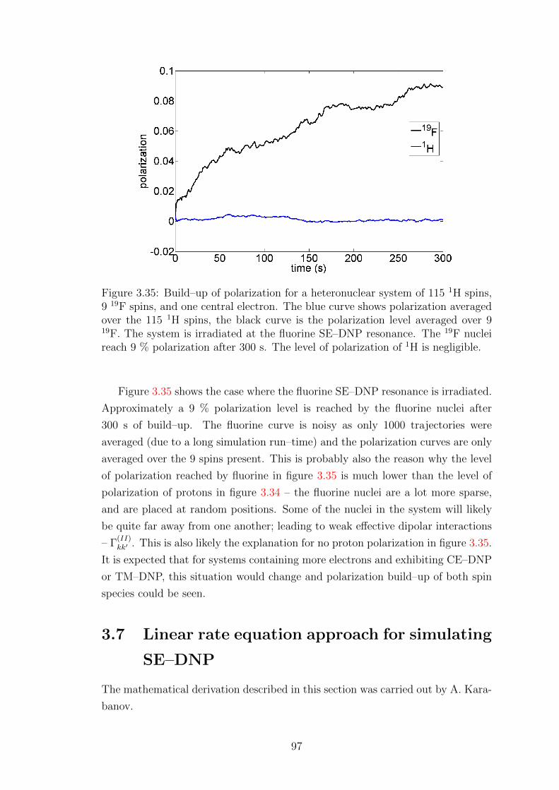
Figure 3.35: Build–up of polarization for a heteronuclear system of 115 1H spins,9 19F spins, and one central electron. The blue curve shows polarization averagedover the 115 1H spins, the black curve is the polarization level averaged over 919F. The system is irradiated at the fluorine SE–DNP resonance. The 19F nucleireach 9 % polarization after 300 s. The level of polarization of 1H is negligible.

Figure 3.35 shows the case where the fluorine SE–DNP resonance is irradiated.

Approximately a 9 % polarization level is reached by the fluorine nuclei after

300 s of build–up. The fluorine curve is noisy as only 1000 trajectories were

averaged (due to a long simulation run–time) and the polarization curves are only

averaged over the 9 spins present. This is probably also the reason why the level

of polarization reached by fluorine in figure 3.35 is much lower than the level of

polarization of protons in figure 3.34 – the fluorine nuclei are a lot more sparse,

and are placed at random positions. Some of the nuclei in the system will likely

be quite far away from one another; leading to weak effective dipolar interactions

– Γ(II)kk′ . This is also likely the explanation for no proton polarization in figure 3.35.

It is expected that for systems containing more electrons and exhibiting CE–DNP

or TM–DNP, this situation would change and polarization build–up of both spin

species could be seen.

3.7 Linear rate equation approach for simulating

SE–DNP

The mathematical derivation described in this section was carried out by A. Kara-

banov.

97

The SE–DNP dynamics enclosed in the zero–quantum subspace of the density

operator – master equation in eq. (3.13) are projected onto the subspace of spin

polarizations, in a manner similar to that seen in section 3.1.3.

The subspace of Zeeman orders covers terms

LZ = span{1, Sz, Ikz, SzIkz, IkzIk′z, . . .},

and LC then covers the complimentary subspace. The subspace containing the

polarization dynamics is a (n+1)–dimensional single–spin Zeeman–order subspace

– in other words it is a subspace within the Zeeman subspace concerning single–

spin coherence orders.

LP = span{Sz, Ikz, Ik′z, . . .

}⊂ LZ .

3.7.1 Projection onto the polarization subspace

The relevant projection superoperator onto the polarization subspace is PP , and

QP is the complimentary projection superoperator. The action of the superoper-

ator L00 is enclosed in LP , and acts on operators Sz, Ikz as follows

L00Sz = −R(S)1

2Sz, L00Ikz = −R

(I)1

2Ikz,

the action of PPM2PP leads to second order correction terms resulting in

Γ′ = −R(S)2 ω2

1

2ω2I

Sz −R

(I)2 |Bk±|2

8ω2I

,

analogous to the relaxation term seen originally for the Zeeman–projected dy-

namics, shown in eq. (3.14) and (3.18). In the same manner as with the Zeeman–

subspace projection, the dynamics of H ′1 and H0 were projected onto the polar-

ization subspace LP

L10 = −iQP(

ˆH ′0 + ˆH ′1

)PP ,

L01 = −iPP(

ˆH ′0 + ˆH ′1

)QP ,

L11 = −i(

ˆH0,0 + ˆH1,0

)+ Γ′.

98

Acting on terms in the polarization subspace these give

L10Sz =iω1

4ωI

∑k

(Bk+Ik+S− −Bk−Ik−S+

),

L10Ikz =iω1

4ωI

∑k

(Bk−Ik−S+ −Bk+Ik+S−

)+i

2

∑k<k′

dkk′(Ik+Ik′− − Ik−Ik′+

),

thus it is accurate to calculate the action of L11 on the operators Ik±S∓, Ik±Ik′∓,

L11

(Ik±S∓

)= Pk±Ik±S∓, Pk± = ±iλ± i

∑s 6=k

AsIsz − (R(I)2 +R

(S)2 ),

L11

(Ik±Ik′∓

)= Pkk′ Ik±Ik′∓, Pkk′ = i(Ak − Ak′)Sz − 2R

(I)2 .

Immediately a resemblance to the form of the effective rates for the Zeeman–

subspace master equation – eq. (3.20) can be seen. In addition, the superoperator

L11 acts trivially on Pk± and Pkk′ , hence

(L11)m(Ik±S∓

)= (Pk±)mIk±S∓,

(L11)m(Ik±Ik′∓

)= (Pkk′)

mIk±Ik′∓,

for m = 1, 2, 3, . . . , and as follows from linear algebra properties

eL11

(Ik±S∓

)= ePk±tIk±S∓,

eL11

(Ik±Ik′∓

)= ePkk′ tIk±Ik′∓.

The operators Ikz commute with each other. From the properties of these opera-

tors, and that of Sz, we get that

ePk±t = e(±iλ−R(I)2 −R

(S)2 )t

∏k′ 6=k

[cos

(Ak′t

2

)± 2i sin

(Ak′t

2

)Ik′z

],

ePkk′ t = e(−R(I)2 −R

(S)2 )t

[cos

((Ak − Ak′)t

2

)± 2i sin

((Ak − Ak′)t

2

)Sz

].

The result of the action of L01 must belong to LZ hence;

L01eL11tIk±S∓ = ePk±tL01Ik±S∓, L01e

L11tIk±Ik′∓ = ePkk′ tL01Ik±Ik′∓.

Using the formulas

L01Ik±S∓ = ±iω1Bk±

4ωI

(Sz − Ikz

), L01Ik±Ik′∓ = ±idkk

′

2

(Ikz − Ik′z

),

99

one obtains

L01eL11tL10Sz = − ω2

1

16ω2I

∑k

|Bk|2(ePk+t + ePk−t

)(Sz − Ikz

)(3.43)

L01eL11tL10Ikz =

ω21

16ω2I

|Bk|2(ePk+t + ePk−t

)(Sz − Ikz

)(3.44)

− 1

4

∑k′ 6=k

(ePk′kt + ePkk′ t

)(Ikz − Ik′z

)Furthermore,

ePk′kt + ePkk′ t = 2e−2R(I)2 t cos

((Ak − Ak′)t

2

),

hence the terms resulting in dipolar flip–flops, i.e. terms proportional to d2kk′ are

enclosed in LP . The terms proportional to |Bk|2 are not. Higher Zeeman orders

are generated due to the presence of the factors(ePk+t + ePk−t

).

This is avoided if the negative eigenvalues of L11 are large due to decoherence

rates; R(I)2 and R

(S)2 . Under the assumptions required for the projection onto the

Zeeman subspace, eq. (3.15) this issue will be avoided, and the dynamics will

remain within the polarization subspace LP of the Zeeman subspace LZ ;

˙ρ = LP ρ.

The result is a set of linear rates describing polarization build–up for nuclear

spins, and the depolarization of the electron spin. The dynamics for each spin are

described analytically as follows

LP Sz = −R(S)1

2Sz −

R(S)2 ω2

1

2ω2I

Sz −∑k

ω21 |Bk|2

8ω2I

Dk

(Sz − Ikz

), (3.45)

LP Ikz = −R(I)1

2Ikz −

R(I)2 |Bk|2

8ω2I

Ikz +ω2

1 |Bk|2

8ω2I

Dk

(Sz − Ikz

)(3.46)

−1

2

∑kk′

d2kk′Ckk′

(Ikz − Ik′z

).

The coefficients Ckk′ and Dk are given as

Ckk′ =

∫ ∞0

e−2R(I)2 t cos

((Ak − Ak′)t

2

)dt, (3.47)

Dk =

∫ ∞0

e−(R(I)2 +R

(S)2 )t cos(λt)

∏k′ 6=k

cos

(Ak′t

2

)dt. (3.48)

100

For the coefficient Ckk, nuclei with a significant coupling strength dkk′ will not have

a difference in secular coupling strengths Ak that is larger than 2R(I)2 , hence this

coefficient will rapidly tend to a steady–state value. The effective rate of inter–

nuclear dipolar flip flops will have the same form as Γ(II)kk′ in eq. (3.23), which has

previously been shown to be state–independent.

The story is slightly different for the coefficient Dk. This coefficient is to com-

pensate for the state–depencence of rate Γ(IS)k in eq. (3.22), manifested in the

state–dependent coefficient, shown in eq. (3.26). There exist systems where Ak

can exceed R(I)2 +R

(S)2 .

The product part of eq. (3.48)

∏k′ 6=k

cos

(Ak′t

2

), (3.49)

causes Dk to be time–dependent due to the oscillatory behaviour of the product

of cosine functions. Using properties of trigonometric functions it can be shown

that the fastest–oscillating part of the product in eq. (3.49) will oscillate with a

frequency of ∼∑

k′ 6=k|Ak|

2. Thus as an upper–bound on the oscillation frequencies

of the product in eq. (3.49) is it reasonable to take∑

kAk2

, and if this term is

much greater than R(I)2 +R

(S)2 , than the coefficient Dk will have a significant time–

dependence in the early stages of the simulation, and its decay to a steady–state

will not be quick enough.

The conditions in eq. (3.15) have to be met to make the projection onto the

polarization subspace accurate, but in addition, the error will likely be large if∑k |Ak|

2(R(I)2 +R

(S)2 )� 1. (3.50)

This has to be avoided in a system of choice.

3.7.2 Error testing against Zeeman projection

With the accuracy of the Zeeman projection established in section 3.2, the linear

rate equation approach was compared to the simulations implemented with the

use of kMC algorithms; for the purpose of an error analysis. A cubic system of 125

spins was chosen, with the electron spin in the centre. The separation between

the nearest–neighbour spins a was varied between 6 A and 10 A. Simulations

were carried out for both 13C and 1H nuclear spins. A 5 % randomization in

the position of spins was applied. The magnetic field BZ was set to 3.4 T, the

relaxation parameters were R(S)1 = 1 s, R

(S)2 = 10 µs, R

(I)1 = 1 h, R

(I)2 = 0.1 ms.

101

The microwave field amplitude ω1 was set to 50 kHz unless otherwise stated.

For a spacing of 10 A the error is negligible – figure 3.36 A, and the fraction on

the LHS of eq. (3.50) is equal to ∼ 8.8. A inter–spin spacing of 9 A results in

a slightly larger but still acceptable error, seen in figure 3.36 B. The fraction in

eq. (3.50) is 12.4 in this case. For spacings of 8 A and 7 A respectively the error

increases each time – figure 3.36 C & D. The sum of secular coupling strengths,

divided by the decoherence rates are in this case 17.6 and 26.1 respectively, thus

more than an order of magnitude greater than 1, and the regime outlined by the

inequality in eq. (3.50) is reached.

Figure 3.36: Errors analysis was carried out for a cube of 124 13C spins surroundingan electron spin. The inter–spin spacing, a is varied. Part A) – a = 10 A, Part B)– a = 9 A, Part C) – a = 8 A, Part D) – a = 7 A. The error for each individualspin is shown. The blue line corresponds to the electron, which typically has thelowest error. The error is seen to increase for stronger spin–spin coupling.

As expected, the error gets worse when the separation is reduced to 6 A, in

figure 3.37 A, where the ratio of the sum of secular coupling strengths to the

decoherence rates is 41.9. This is then compared to a simulation of the same

system with hydrogen nuclei, where ω1 = 160 kHz. Protons have a much higher

gyromagnetic ratio than 13C nuclei, hence the error in figure 3.37 B is even higher.

The ratio of the sum of the secular coupling strengths to R(S)2 + R

(I)2 is 165.2 in

this case.

102

Figure 3.37 C shows the simulation outcome for 13C nuclei with a = 6 A, but the

decoherence rate R(S)2 increased to 106 (s−1), as a comparison to figure 3.37 A.

The error falls below 2 % for all spins other than the electron, as the ratio from

eq. (3.50) is now reduced from 41.9 to 4.6.

Figure 3.37: Error analysis carried out for cubic lattices of 124 1H or 13C nuclearspins surrounding a central electron. The error for each spin is shown; the blueline corresponds to the the electron spin and the rest corresponds to the nuclearspins. Part A) simulation for 13C where a = 6 A, Part B) simulation for 1H wherea = 6 A ω1 = 160 kHz. For 1H nuclei, which have stronger coupling, the erroris significantly larger. Part C) simulation for 13C with a = 6 A and the rate of

electronic decoherence increased (T(S)2 = 1 µs). For shorter decoherence times the

error is reduced as the condition in eq. (3.50) is met again.

3.7.3 Very large spin–system simulations

Having established the parameter region where the formalism of the linear effective

rates is accurate; a simulation was carried out on a spin system containing 9261

spins. The model system is a cube of dimension 21× 21× 21. A spacing of 10 A

was set between nearest spins, with a 5 % randomization in position of all spins.

The magnetic field Bz was set to 3.4 T, the microwave field amplitude ω1 = 250

kHz, and the following relaxation parameters were chosen: T(S)1 = 20 ms, T

(S)2 =

10 µs, T(I)1 = 1 h, T

(S)2 = 0.1 ms.

103

The simulation took 450 seconds, thus illustrating the power and efficiency of the

linear rate formalism, in eqs. (3.45), (3.46).

Nuclear polarization is normalised to the electronic thermal polarization. The

system in figure 3.38 is seen to reach an average level of 11 % of polarization

after 1 hour of microwave irradiation. The time–shot parts of figure 3.38 show the

diffusive transport of polarization to the bulk, and the high level of polarization

reached by the core. A spin system of this size is expected to suffer a lot less from

a reflective boundary, and in addition, periodic boundary conditions to imitate a

sample with a number of spins on the order of Avogadro’s constant could most

likely be considered.

Figure 3.38: Large spin system simulation showing the build–up of polarizationfor a cubic lattice of 9260 13C nuclei surrounding a central electron spin. The firstpart shows the mean nuclear polarization as a function of time. The system isseen to reach steady–state after a time of 5 h, with a polarization level of ∼ 15 %.Time shots illustrating polarization of individual spins, at 900 s, 1800 s, and 3600s are also shown. These clearly demonstrate diffusive transport from core nucleito the bulk.

104

Chapter 4

Radical design

In this chapter the dependence of nuclear polarization during DNP build–up on the

geometrical configuration of the system is studied. The study is carried out using

a model central spin system, consisting of an electron surrounded by many nuclei

and exhibiting SE–DNP. It’s made feasible by the use of the kinetic Monte Carlo

method, which allows one to significantly increase the number of spins considered

in the model system. Our findings demonstrate that increasing the minimal dis-

tance between nuclei and electrons leads to a rise of the nuclear bulk polarization.

These observations therefore have implications for the design of radicals that can

lead to improved bulk nuclear spin polarization.

This chapter largely follows the work published by us in [59].

4.1 Introduction

The formalism described in section 3.1 opens up the possibility of analysing polar-

ization transport in systems of up to a few thousand coupled spins. The focus of

this chapter is on the insight that such simulations can provide in understanding

the dynamics of large, uncoupled spin ensembles during DNP. In particular, it is

shown how the bulk polarization level crucially depends on the immediate molec-

ular environment of the unpaired electron spin.

The effective rates can be used to distinguish between bulk and core nuclei. Com-

parison between the two rates (Γ(IS)k and Γ

(II)kk′ ) for each nucleus determines whether

it belongs to the core or to the bulk. In the case that the effective hyperfine rate,

eq. (3.24), is greater than the effective nuclear dipolar rate (Γ(IS)k > Γ

(II)kk′ ), eq.

(3.25), the interaction with the electron will be dominating, indicating a core

nucleus. The opposite would be true (Γ(IS)k < Γ

(II)kk′ ) for a bulk nucleus.

105

4.2 Model spin system

Large spin–system simulations were carried out in order to gain further insight

into the optimal conditions for SE–DNP, for achieving the highest nuclear spin

polarization and the fastest build–up rate of nuclear polarization. This kind of

analysis provides important information for a tailored radical design in which

radical compounds would be synthesized with desired properties. In this context,

that would correspond to an optimal separation between the electron radical,

and the nuclear spins closest to it, as well as on the geometry of the molecule

containing the electron radical. In order to analyse the spin dynamics during SE–

DNP, a system of one central electron surrounded by 13C nuclear spins arranged

in a 5×5×5 cubic grid was chosen – thus consisting of a total of 124 nuclear spins.

The nearest neighbour separation between nuclear spins was set to 4 A, and a

1% uniform randomization in position of each spin was applied. Such an average

distance between nuclei corresponds to 26 M of a 13C labelled molecule or in other

words – it is slightly shorter then the average distance between 13C nuclei in free

pyruvic acid (4.8 A) [60]. The magnetic field was set to be 3.4 T, the temperature

was set 1K, and a microwave field amplitude of 20 kHz was chosen to approximate

realistic experimental conditions (without the use of a gyrotron microwave source

or a resonance cavity). The relaxation parameters were set to be: T(S)1 = 0.5 s,

T(S)2 = 10 µs, T

(I)1 = 1 h, T

(I)2 = 0.5 ms. The polarization dynamics during one

hour of microwave irradiation were simulated using our effective rate formalism

and a kMC algorithm.

In order to better understand the dependence on polarization build–up on the

coupling parameters, these were plotted as a function of position in space. Figs. 4.1

and 4.2 show the spatial dependence of the secular and pseudo–secular hyperfine

interaction strengths Ak and Bk for the 124 13C nuclei. The rate in eq. (3.24)

shows a squared dependence on Bk± i.e. the pseudo–secular hyperfine coupling

strength. It is therefore reasonable to expect that nuclei with the highest Bk±

values will have the highest effective rate Γ(IS)k values.

On the other hand, nuclei with the highest Ak will be shifted in frequency the

most, due to the interaction with the electron. The rate in eq. (3.25) will be lower

between nuclei that have a large difference in their secular coupling strengths. The

efficiency of SE–DNP for the nuclear ensemble, seen in terms of build–up duration

and steady–state polarization level, will rely on a delicate interplay between these

two processes.

106

Figure 4.1: Strength of the secular hyperfine interaction Ak between the centralelectron (black) and the 124 13C nuclei. The colour scale indicates the couplingstrength in kHz. Note the non–uniform scale of the colour bar.

Figure 4.2: Strength of the pseudo–secular hyperfine interaction Bk between thecentral electron (black) and the 124 13C nuclei. The colour scale indicates thecoupling strength in kHz. Note the non–uniform scale of the colour bar.

The magnitudes of the secular part and the pseudo–secular part of the hyper-

fine interaction (previously shown in 2.2) are given by

107

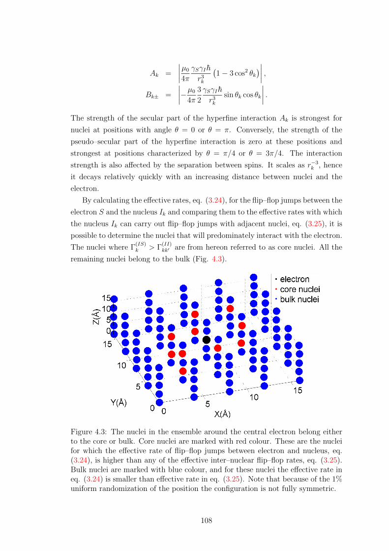
Ak =

∣∣∣∣µ0

4π

γSγI~r3k

(1− 3 cos2 θk

)∣∣∣∣ ,Bk± =

∣∣∣∣−µ0

4π

3

2

γSγI~r3k

sin θk cos θk

∣∣∣∣ .The strength of the secular part of the hyperfine interaction Ak is strongest for

nuclei at positions with angle θ = 0 or θ = π. Conversely, the strength of the

pseudo–secular part of the hyperfine interaction is zero at these positions and

strongest at positions characterized by θ = π/4 or θ = 3π/4. The interaction

strength is also affected by the separation between spins. It scales as r−3k , hence

it decays relatively quickly with an increasing distance between nuclei and the

electron.

By calculating the effective rates, eq. (3.24), for the flip–flop jumps between the

electron S and the nucleus Ik and comparing them to the effective rates with which

the nucleus Ik can carry out flip–flop jumps with adjacent nuclei, eq. (3.25), it is

possible to determine the nuclei that will predominately interact with the electron.

The nuclei where Γ(IS)k > Γ

(II)kk′ are from hereon referred to as core nuclei. All the

remaining nuclei belong to the bulk (Fig. 4.3).

Figure 4.3: The nuclei in the ensemble around the central electron belong eitherto the core or bulk. Core nuclei are marked with red colour. These are the nucleifor which the effective rate of flip–flop jumps between electron and nucleus, eq.(3.24), is higher than any of the effective inter–nuclear flip–flop rates, eq. (3.25).Bulk nuclei are marked with blue colour, and for these nuclei the effective rate ineq. (3.24) is smaller than effective rate in eq. (3.25). Note that because of the 1%uniform randomization of the position the configuration is not fully symmetric.

108

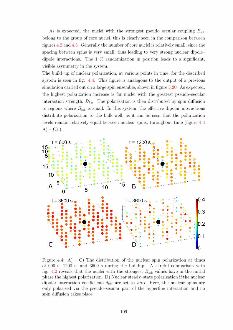
As is expected, the nuclei with the strongest pseudo–secular coupling Bk±

belong to the group of core nuclei, this is clearly seen in the comparison between

figures 4.2 and 4.3. Generally the number of core nuclei is relatively small, since the

spacing between spins is very small, thus leading to very strong nuclear dipole–

dipole interactions. The 1 % randomization in position leads to a significant,

visible asymmetry in the system.

The build–up of nuclear polarization, at various points in time, for the described

system is seen in fig. 4.4. This figure is analogous to the output of a previous

simulation carried out on a large spin ensemble, shown in figure 3.20. As expected,

the highest polarization increase is for nuclei with the greatest pseudo–secular

interaction strength, Bk±. The polarization is then distributed by spin diffusion

to regions where Bk± is small. In this system, the effective dipolar interactions

distribute polarization to the bulk well, as it can be seen that the polarization

levels remain relatively equal between nuclear spins, throughout time (figure 4.4

A) – C) ).

Figure 4.4: A) – C) The distribution of the nuclear spin polarization at timesof 600 s, 1200 s, and 3600 s during the buildup. A careful comparison withfig. 4.2 reveals that the nuclei with the strongest Bk± values have in the initialphase the highest polarization. D) Nuclear steady–state polarization if the nucleardipolar interaction coefficients dkk′ are set to zero. Here, the nuclear spins areonly polarized via the pseudo–secular part of the hyperfine interaction and nospin diffusion takes place.

109

Several nuclei closest to the electron clearly show a lower polarization level than

the remainder. These are the nuclei with the highest secular coupling strength

(see figure 4.1). Part B) of figure 4.4 shows that the two nuclei directly above and

below the electron have a much lower polarization level. These two nuclei have

the highest Ak values. The remaining 4 closest nuclei in plane with the electron

have a secular value 2 times smaller than that, yet they still show a lower degree

of polarization in comparison to the bulk. It thus becomes clear that nuclei with

low Bk± values and high Ak are a hindrance to the mechanism of polarization

transport to the bulk. The contributions of the effective dipolar rate Γ(II)kk′ can be

seen in figure 4.4 D). There the effective rate for internuclear flip–flops was set to

zero during the course of the simulation. In such case only nuclei in regions with

Bk± 6= 0 receive significant electronic polarization during SE DNP.

4.3 Influence of nuclei close to the electron

The result in figure 4.4 shows that some nuclei might be reducing the efficiency

with which polarization is transferred to the bulk. In our study we analysed the

effect on the average bulk polarization under changes to the configuration of this

model system. The six nuclei which are the nearest neighbours to the electron spin,

hence ones with the highest secular hyperfine interaction strength (Ak) were first

removed in succession. The simulation was re–run starting from the initial thermal

equilibrium state, upon removal of each nucleus from the system, in order to study

the effect this had on the bulk polarization. The polarization level at steady–

state, so after 1 hour of build–up was calculated each time. Following removal

of the nearest neighbouring nuclei, further nuclei adjacent to the electron were

subsequently removed. A study as such would of course not be possible without

many–body system simulations, made possible by the effective Zeeman–subspace

master equation and efficient kMC algorithms. The idea here is to understand the

role of the secular and pseudo–secular terms of the hyperfine interaction of nuclei

in immediate proximity of the electron on spin–diffusion and hence on the bulk

nuclear polarization. Fig. 4.5 shows the order and the position of the removed

nuclei. The dependence of the mean nuclear spin polarization per nucleus at steady

state, on the number of removed nuclei is summarized in fig. 4.6. The nuclei

are removed in the sequence depicted in figure 4.5. The first data point (black)

represents the average nuclear spin polarization in the system without removal

of any nuclei. The next six data points (dark blue) indicate the average nuclear

spin polarization if the six nuclei with the strongest secular hyperfine interaction

strength Ak are successively removed.

110

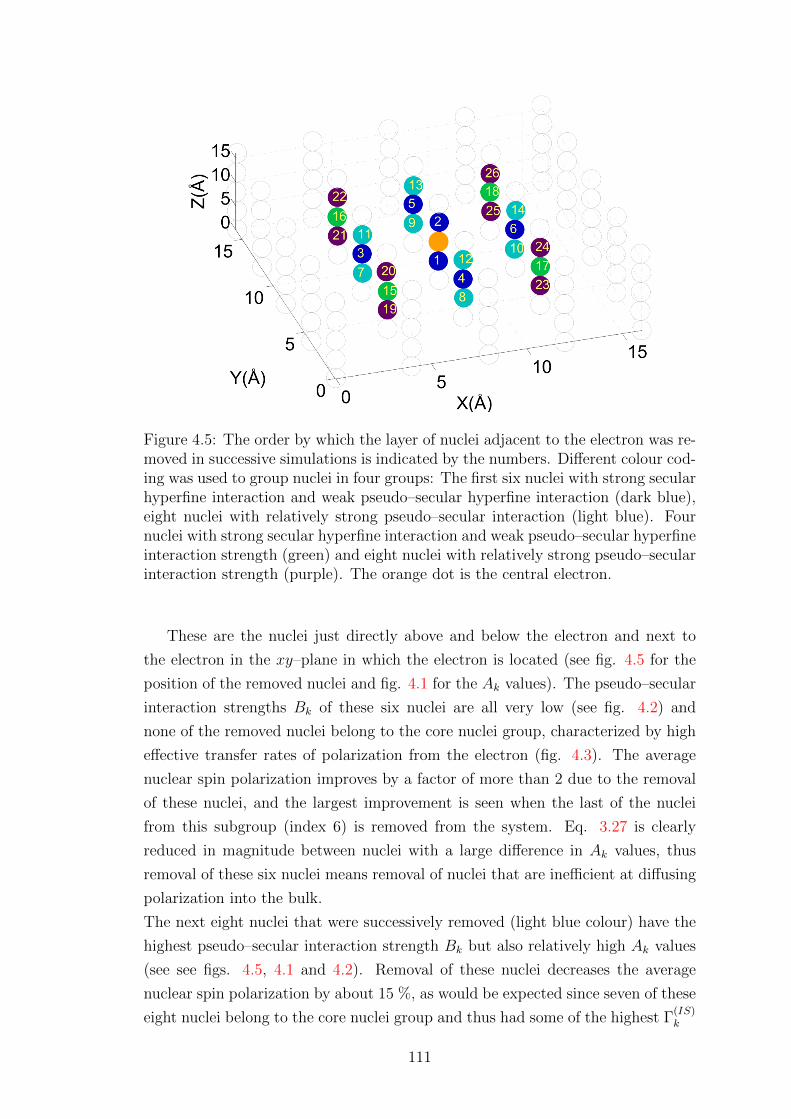
Figure 4.5: The order by which the layer of nuclei adjacent to the electron was re-moved in successive simulations is indicated by the numbers. Different colour cod-ing was used to group nuclei in four groups: The first six nuclei with strong secularhyperfine interaction and weak pseudo–secular hyperfine interaction (dark blue),eight nuclei with relatively strong pseudo–secular interaction (light blue). Fournuclei with strong secular hyperfine interaction and weak pseudo–secular hyperfineinteraction strength (green) and eight nuclei with relatively strong pseudo–secularinteraction strength (purple). The orange dot is the central electron.

These are the nuclei just directly above and below the electron and next to

the electron in the xy–plane in which the electron is located (see fig. 4.5 for the

position of the removed nuclei and fig. 4.1 for the Ak values). The pseudo–secular

interaction strengths Bk of these six nuclei are all very low (see fig. 4.2) and

none of the removed nuclei belong to the core nuclei group, characterized by high

effective transfer rates of polarization from the electron (fig. 4.3). The average

nuclear spin polarization improves by a factor of more than 2 due to the removal

of these nuclei, and the largest improvement is seen when the last of the nuclei

from this subgroup (index 6) is removed from the system. Eq. 3.27 is clearly

reduced in magnitude between nuclei with a large difference in Ak values, thus

removal of these six nuclei means removal of nuclei that are inefficient at diffusing

polarization into the bulk.

The next eight nuclei that were successively removed (light blue colour) have the

highest pseudo–secular interaction strength Bk but also relatively high Ak values

(see see figs. 4.5, 4.1 and 4.2). Removal of these nuclei decreases the average

nuclear spin polarization by about 15 %, as would be expected since seven of these

eight nuclei belong to the core nuclei group and thus had some of the highest Γ(IS)k

111

rates.

The next four nuclei (green) that were removed have high Ak values and low

Bk values. The removal of these nuclei increases again the average nuclear spin

polarization of the ensemble. Following the removal of these nuclei, the nuclei

left remaining in the system have more efficient polarization exchange rates, Γ(II)kk′ .

Compared to the polarization level of the last bright blue data point (spin index

number 14) the increase is more than 30 %.

Figure 4.6: Mean polarization per nucleus versus the number of nuclei removedfrom the model system. The colour coding is identical to the one used in fig.4.5. The first data point corresponds to the mean polarization without any nucleiremoved (black). The next six data points (dark blue) correspond to the meanpolarization if the six nuclei with strongest secular hyperfine interaction strengthAk are removed. The next eight data points (light blue) correspond to the meanpolarization if nuclei with strong pseudo–secular interaction strength are removed(Bk). The next four data points again correspond to removal of nuclei with highAk values and the final eight data points (purple) correspond to removal of nucleiwith high Bk values. The broken black line has been added as a visual guide.

This polarization level compared to the average polarization for the reference

system without any nuclei removed, shows that the polarization of this system

(marked by spin index number 19 in figure 4.5) is increased by more than a factor

of 2.3. The last eight nuclei that were removed have high Bk values and the

average nuclear spin polarization level decreases by about 10%.

In order to interpret these results it is instructive to analyse the distribution

of frequencies which are characteristic for SE–DNP. The effect of the nuclei with

112

strong secular hyperfine interaction (high Ak values) is a splitting of the frequencies

ωS ± ωI at which SE–DNP is mediated by an excitation of ZQ or DQ transitions

[61, 37]. The splitting of these frequencies for each nucleus Ik can be calculated

by using [61, 37]

ωDNPIk= ωS ± ωI −

1

2

∑i 6=k

siAi, si = ±1, (4.1)

where si is a sum implying that one needs to add up over both of the possible

permutations. In order to calculate the splitting frequencies for a given nucleus,

one needs to sum over all permutations of all other spins. This means that for a

system of n nuclei the total number of DNP frequencies is 124 × 2(n−1) – a number

that is not computationally feasible. Because the number of transition frequencies,

resulting from the coupling of 124 nuclei to the electron is extremely high, we

have selected only 25 nuclei to calculate these frequencies. These were chosen

by ordering all nuclei according to secular coupling strength, Ak, in a decreasing

order. The first 25 nuclei with the highest Ak values were then selected each time,

reducing the number of frequencies to a more feasible value. The distributions of

frequencies calculated using eq. (4.1) are shown in histograms (see fig. 4.7). The

histograms are plotted for systems with 0, 2, 6, 14, 18, and 24 nuclei removed,

respectively. In these histograms the fractional number of transition frequencies

at which nucleus–electron flip–flops occur are plotted against the frequency offset

with respect to the ZQ frequency ωS + ωI .

With the removal of the first six nuclei the distribution becomes significantly

narrower – these have the largest effect on the width of the distribution of the SE–

DNP frequencies. Further removal of nuclei reduces the width of the distribution

less significantly, until the Ak values of the removed nuclei are so weak that no

further significant change is observed. From fig. 4.7 we can conclude that initially

the successive removal of nuclei with strong secular coupling causes a larger number

of nuclei to have transition frequencies closer to the microwave carrier frequency,

set to ωS+ωI and hence SE–DNP will be more efficient. However, while this has a

positive effect on the average nuclear spin polarization, removal of nuclei with high

Bk values that can transfer polarization to the bulk by spin diffusion, does have

a negative effect on the average nuclear spin polarization. These considerations

show the delicate interplay between the various parameters in the spin ensemble,

controlled by the geometry of the system.

113

Figure 4.7: Histograms show the distribution of frequencies for ZQ transitions thatoccur in the model spin ensemble. The frequencies are given as offset frequenciesin respect to the ZQ transition ωS + ωI . The nuclei are successively removed(none, 2, 6, 14, 18 and 24 removed) and the frequencies for ZQ transitions arecalculated. The first two nuclei with the strongest secular hyperfine interactionAk were removed, leading to a significant narrowing of the distribution. Removalof the next 4 nuclei then very visibly narrows the distribution of frequencies fur-ther. Additional nuclei were then subsequently removed, in an order of descendingsecular hyperfine interaction strength. Fig 4.5 shows the positions of the removednuclei. Generally the width of the distribution becomes narrower with increasingnumbers of nuclei removed. However, the six nuclei that were removed at the endhave only very weak Ak values, and there is no significant change between the lasttwo histograms.

Our simulation results demonstrate that the average nuclear spin polarization

is more than 2 times higher if the 26 nuclei adjacent to the central electron are

removed. The removal of the nuclei means that nearest distance between nuclei

and electron has increased by a factor of 2. The separation between the electron

and nearest nuclei is now 8 A, while the separation between neighbouring nuclear

114

spins is still 4 A. This is somewhat analogous to increasing the volume occupied

by the molecule containing the electron radical. The expulsion volume for nuclei

could be implemented by designing radical molecules with additional functional

groups.

If further layers of nuclei were removed it is to be expected that the average nuclear

spin polarization would decrease to levels below the initial level, i.e. that of the

system without any nuclei removed, since the pseudo–secular interaction strength

would become too weak for an efficient polarization transfer between the central

electron and the interacting nuclei. From these considerations it is clear that there

must be a set of parameters that gives the optimum DNP efficiency; parameters

for which the build–up time would be the shortest, and for which the nuclear

spin polarization will reach its highest level. Such an optimum does depend in a

complex way on all parameters including the microwave irradiation strength, the

average distance between the nuclei, the nearest distance between nuclei and the

central electron, and the various R1, R2 relaxation parameters.

4.4 Radical design

The simulations and the results presented in this work point to a possible expla-

nation why the trityl radical, currently in frequent use for 13C dissolution DNP,

seems to perform particularly well [62, 63]. The explanation is based on the as-

sumption that there is also an optimal distance for CE–DNP between the electron

and the nuclei.

The bulky aromatic groups of the tritly compound keep the molecules that carry

the 13C–label (e.g. [1− 13C] pyruvate) at an appreciable distance to the electron

(analysis for 1H nuclei was carried out in [64]). The relatively large separation

between 13C nuclei and the electron results in a relatively narrow distribution of

the possible DNP transition frequencies in the nuclear spin ensemble. The 13C

nuclei are, however, still near enough to ensure a high pseudo–secular interaction

between the first layer of nuclei and the electron. Furthermore, the large sepa-

ration between the electron spin and the nearest layer of nuclei will result in a

lower difference between the secular hyperfine interaction strengths of adjacent

nuclei as opposed to a case of a radical with a smaller steric factor – allowing

nuclei to get very close to the electron spin. This in turn will lead to more efficient

spin diffusion (rate eq. (3.25)) between nuclei closest to the electron and those in

the next layer – further away – meaning polarization will be transported through

the lattice more rapidly. These considerations demonstrate that the performance

of DNP is critically dependent on the immediate molecular environment of the

115

paramagnetic centre and that improvements in the performance of DNP could be

obtained by a precise radical design.

116

Chapter 5

Cross Effect

5.1 Effective Cross Effect dynamics

This chapter focuses on cross effect DNP. The theory is already described in chap-

ter 2. In this section the adiabatic elimination and projection of the CE-DNP

dynamics onto the Zeeman subspace of the density operator is described - the

original derivation of the effective dynamics was carried out by A. Karabanov.

The effective dynamics and the parameters they depend on are then described

in great detail. This is followed by a comprehensive error analysis, spin diffusion

studies in 1D systems, optimisation studies for bi-radicals, and finally large spin

ensemble simulations. The research described in this chapter is not yet published

as of the time of writing.

It is also to be noted that the relaxation rates of T1 and T2 for both electron spins

have been chosen to be identical, however this is not a requirement and can be

altered at will. The same applies to the relaxation rates for the nuclei - there can

be variation in T(I)1 and T

(I)2 values of the system.

5.1.1 Elimination of non-zero quantum coherences

The CE–DNP dynamics are projected onto the diagonal part of the density op-

erator, the so–called Zeeman subspace, in a two–step process. The resonance

condition for the cross effect, outlined in 2.3.1 indicates that the mechanism of

transfer of polarization to the nuclear spins is optimal when one of the electrons

has their EPR transition saturated; i.e. the microwave radiation is on resonance

with its Larmor frequency.

Thus by projecting the dynamics at the CE–DNP resonance condition, the dynam-

ics are projected onto the zero–quantum subspace of the off–resonance electron and

the nuclear spins. Subsequently the derived dynamics are then projected onto the

117

Zeeman subspace of this zero–quantum subspace. In effect, the relevant subspace

dimension of the density operator is reduced from 4(n+2) to 2(n+2) for n nuclear

spins. The general mathematical procedure of adiabatic elimination is explained

in great detail in section 2.4.

The CE–DNP Hamiltonian for a single electron pair and n nuclei is shown in 2.22.

For convenience, the rotating–frame Hamiltonian is separated into four parts

H = HZ

+ H0 + H+ + H−,

where

HZ = ∆1S(1)z + ∆2S

(2)z +

∑k

ωI Ikz

H0 = λ2S(2)z + λ1

(S(1)z + S(2)

z

)+ 2DS(1)

z S(2)z +

∑k

A(1)k IkzS

(1)z

+ω1

2

(S

(1)+ + S

(1)−

)+∑k

A(2)k IkzS

(2)z +

∑k<k′

(2Ikz Ik′z − Ik · Ik′

)H± =

ω1

2S

(2)± −

D

2S

(2)± S

(1)∓ +

1

2

2,n∑j,k

B(j)k±Ik±S

(j)z ,

with offset terms ∆1,∆2, which are ∆j = ω(j)S − ωµw, i.e. the difference between

the Larmor frequency of an electron and the microwave field frequency.

At the CE–DNP resonance, ∆1 ≈ 0 and ∆2 ≈ ±ωI , hence the Zeeman Hamilto-

nian becomes HZ = ωI

(±S(2)

z +∑

k Ikz

). The offset terms from this CE–DNP

resonance condition are λ1, λ2. Their form is λ1 = ∆1, λ2 = ∆2 −∆1 − ωI .

The terms HZ , H0 keep dynamics of a particular subspace enclosed in that sub-

space. Terms H±, on the other hand, cause cross–overs between the different

subspaces.

The system is also subject to dissipation. There is longitudinal relaxation driv-

ing all spins back to their thermal equilibrium, and there are also decoherence

processes. The dissipator for this system is written as

Γ =∑j

(Γ

(S)+ D[S

(j)+ ] + Γ

(S)− D[S

(j)− ] + Γ(S)

z D[S(j)z ])

+∑k

(Γ

(I)k+D[Ik+] + Γ

(I)k−D[Ik−] + Γ

(I)kz D[Ikz]

),

118

with associated rates

Γ(S)± =

R(S)1

2(1∓ pth) Γ(S)

z = 2R(S)2

Γ(I)k+ = Γ

(I)k− =

R(I)1

2Γ

(I)kz = 2R

(I)2 . (5.1)

The evolution of the system is then described by the Liouville von Neumann

equation˙ρ = (−i ˆH + Γ)ρ. (5.2)

The Liouville state space can be decomposed as

L =∑Lq,

where Lq is the subspace of q–quantum coherences,

ˆHZ ρ = qωI ρ, ρ ∈ Lq, q = 0, ±1, . . . , ±(n+ 1). (5.3)

The case of q = 0, i.e. when ˆHZ ρ = 0 denotes the zero–quantum subspace of the

electron (at offset ∆2 = ωI) and the nuclear spins. The subspace of interest is

therefore the one that commutes with the Zeeman Hamiltonian. The dynamics in

this subspace are a lot slower than the dynamics in the other subspaces, since at

high field

ωI � D,Ak, Bk±, dkk′ ,Γ(S)z ,Γ

(S)± ,Γ

(I)kz ,Γ

(I)k±. (5.4)

Letting the subspace H0 be the zero–quantum subspace, and H1 the complimen-

tary subspace

H0 = L0, H1 =∑q 6=0

Lq,

the relations

(−i ˆH0 + Γ)Lq ⊂ Lq, ˆH± Lq ⊂ Lq±1

along with (5.3) give the following properties

L00ρ0 = −i ˆH0 + Γρ0, L10ρ0 = −i( ˆH+ + ˆH−)ρ0,

L01L±1 = −i ˆH∓ L±1, L01Lq = 0, |q| > 1,

L11L±1 = −(±iωI1 + i ˆH0 + i ˆH± − Γ)L±1,

L11Lq = −(iqωI1 + i ˆH0 + i ˆH+ + i ˆH− − Γ)Lq, |q| > 1.

(5.5)

Due to the presence of relaxation, the eigenvalues of the superoperator L11 have

negative real parts, ζ−, thus the solution in H1 rapidly tends to a steady–state.

Therefore, the condition outlined in section 2.4 is satisfied, and the Kernel func-

119

tion is well approximated by its time–independent steady–state form. The zero–

quantum master equation is well approximated by

˙ρ0 = (L00 + M) ρ0,

where M ≡ −L01L−111 L10.

5.1.2 Superoperator M

In order to find the explicit form of M, the properties of superoperators sum-

marised in eq. (5.5) were used. Superoperator L01 acting on ρ0 leaves the dynamics

in the first quantum coherence subspace L±1

L10ρ0 = −i( ˆH+ + ˆH−)ρ0.

Letting X = L−111 L10ρ0, it is clear that

L11X = L10ρ0 = −i(

ˆH+ + ˆH−

)ρ0.

Therefore, since ωI � (H0,±,D), X can be expanded as a rapidly–converging

power series, truncated to second order. This is carried out in a similar fashion to

that in the case of SE–DNP, shown in section 3.1.2.

As before, the superoperator M is found as a series

M = ω−1I M1 + ω−2

I M2 + . . . (5.6)

converging exponentially fast

M−m∑k=1

ω−kI Mk ∼ εm+1 (ε� 1),

with terms

M1 = −i[ ˆH+,ˆH−], M2 = − ˆH+(i ˆH0 − Γ) ˆH− − ˆH,−(i ˆH0 − Γ) ˆH+, . . . (5.7)

It follows from (5.5) that

ζ− > |ωI |, ‖L01‖ ≤ max ‖ ˆH ±‖, ‖L10‖ ≤ 2 max ‖ ˆH ±‖.

Hence, because of eq. (5.4), equation (5.2) can be replaced by its adiabatic ap-

proximation˙ρ = L0ρ (5.8)

120

with

L0 = L00 + M = M0 + ω−1I M1 + ω−2

I M2,

where

M0 = −i ˆH0 + Γ.

5.1.3 Elimination of non–Zeeman spin orders

Following the procedure from the initial Liouvillian L, eq. (5.2), to the Liouvillian

L0, in eq. (5.8), a master equation accurately describing the dynamics closed in

the subspace H0 is obtained. In this section, the procedure of projection of the

dynamics within zero–quantum subspace onto the Zeeman subspace is described.

This projection results in classical–like dynamics concerning the diagonal elements

of the density operator.

The zero–quantum subspace is decomposed as

L0 = LZ + LC ,

where

LZ = span{1, S(1)z , S(2)

z , Ikz, S(1)z S(2)

z , S(1)z Ikz, . . .},

is the subspace of Zeeman spin orders, and LC the complementary subspace con-

sisting of non–Zeeman, zero–quantum coherences.

The commutation character of the notation ˆO ≡ [O, ·] implies that the super-

operator M1 is a commutation (mathematical proof in appendix A.1):

M1 = −i ˆH1, H1 = [H+, H−] = H1,0 + H ′1,

H1,0 =ω2

1

2S(2)z + ωI

∑k

(bk0 + bk1S1zS2z

)Iz +

D2

4

(S2z − S1z

)H ′1 = −ω1

4

(B

(2)k+S

(2)− Ik+ +B

(2)k−S

(2)+ I−

)− Dω1

2

(S

(1)+ + S

(1)−

)S(2)z

+D

4

[(B

(2)+ −B

(1)+

)S

(1)+ S

(2)− Ik+ +

(B

(2)− −B

(1)−

)S

(1)− S

(2)+ Ik−

],

where bk0 and bk1 are:

bk0 =1

8ωI

(∣∣∣B(1)k

∣∣∣2 +∣∣∣B(2)

k

∣∣∣2) , bk1 =1

2ωI

(B

(1)k+B

(2)k− +B

(1)k−B

(2)k+

).

We have also

H0 = H0,0 + H ′0, Γ = Γ0 + Γ′,

121

where

H0,0 = λ1S(1)z + (λ1 + λ2) S(2)

z + 2DS(1)z S(2)

z +∑j,k

A(j)k S(j)

z Ikz + 2∑k,k′

dk,k′ Ikz Ik′z

H ′0 =ω1

2

(S

(1)+ + S

(1)−

)− dkk′

2

(Ik+Ik′− + Ik−Ik′+

),

and

Γ0 =∑j

R(S)2 D[S(j)

z ] +∑k

R(I)2 D[Ikz],

Γ′ =∑j

{R

(S)1

2(1− pth)D[S

(j)+ ] +

R(S)1

2(1 + pth)D[S

(j)− ]

}

+∑k

R(I)1

2

(D[Ik+] + D[Ik−]

). (5.9)

In agreement with previous notation, 2.4,

L0,kj = πkL0πj, k, j = 0, 1 ,

π0 = PZ , π1 = QC ,

where PZ , QC are projections onto the subspaces LZ ,LC respectively.

The superoperators ˆH0,0,ˆH1,0, Γ0 trivially act on LZ . Within the accuracy of

∼ ω−1I , only the superoperators ˆH

′0, ˆH

′1 contribute to L0,10, L0,01, since

PZM2QC , QCM2PZ � ˆH ′0,ˆH ′1

and thus the terms that scale as ω−2I are negligible. The same applies toQCM2QC ,

hence the superoperator

X = −i ˆH 0,0 + Γ0

maps LC to itself with eigenvalues ζ ′k satisfying

Re ζ ′k < 0, |ζ ′k| > min{2R(I)2 , R

(S)2 +R

(I)2 }.

Thus, under the conditions

1) max(

eig(T0) · eig(Y0))� 1, 2) max

(eig(T2k) · eig(Y2k)

)� 1,

3) max(

eig(T3k) · eig(Y3k))� 1, 4) max

(eig(Tkk′) · eig(Ykk′)

)� 1,(5.10)

122

the subspace LC is adiabatically eliminated and we come then to the approxima-

tion for eq. (5.8),

˙ρZ

= LZρZ , LZ = L0,00 − L0,01L0,11−1L0,10, (5.11)

closed in the Zeeman subspace LZ . Using the fact that ||ω−1I

ˆH0,±||, ||ω−1I Γ|| � 1,

and assuming conditions (5.10), it can be shown that the right–hand side of (5.11)

is well approximated as

L0,11 = Γ′ + Γ′′,

−L0,01L0,11−1L0,10 = T0

ˆY 20

∑k

(T2k

ˆY 22k + T3k

ˆY 23k

)+∑k<k′

Tkk′ˆY 2kk′ ,

(5.12)

where Γ′ is given by eq. (5.9), and Γ′′ is obtained from PZM2PZ ;

Γ′′ =ω2

1R(S)2

2ω2I

(D[S+] + D[S+]

)+R

(S)2 D2

ω2I

(D[K+] + D[K−]

)+R

(I)2

ωI

∑k

(bk0 + bk1S

(1)z S(2)

z

)(D[Ik+] + D[Ik−]

), (5.13)

and

Y0 =ω1

2

(1− D

ωIS(2)z

)(S

(1)+ + S

(1)−

),

Y2k = − ω1

4ωI

(B

(2)k+S

(2)− Ik+ +B

(2)k−S

(2)+ I−

),

Y3k =D

4ωI

[(B

(2)+ −B

(1)+

)S

(1)+ S

(2)− Ik+ +

(B

(2)− −B

(1)−

)S

(1)− S

(2)+ Ik−

],

Ykk′ =dkk′

2(Ik+Ik′− + Ik−Ik′+),

T0 =R

(S)2(

R(S)2

)2

+ P 20

, T2k =R

(I)2 +R

(S)2(

R(I)2 +R

(S)2

)2

+ P 22k

,

T3k =R

(I)2 + 2R

(S)2(

R(I)2 + 2R

(S)2

)2

+ P 23k

, Tkk′ =2R

(I)2(

2R(I)2

)2

+ P 2kk′

,

(5.14)

with the state–dependent coefficients written out explicitly as

123

P0 = λ1 −D2

4ωI+ 2DS(2)

z +∑k

(A

(1)k + bk1S

(2)z

)Ikz,

P2k = λ1 + λ2 +2ω2

1 +D2

4ωI− bk0 +

(2D − A(1)

k

)S(1)z +

∑s 6=k

A(2)s Isz,

P3k = λ2 +ω2

1 +D2

2ωI− bk0 +

bk1

4+∑s 6=k

(A(2)s − A(1)

s

)Isz,

Pkk′ = bk0 − bk′0 + (bk1 − bk′1) S(1)z S(2)

z +2∑j=1

(A

(j)k − A

(j)k′

)S(j)z .

(5.15)

The advantage of formulas (5.12), (5.14) is that they reduce the inversion of L0,11−1

in the subspace LC to the much simpler problem of inversions of the Zeeman

operators T0, T2k, T3k, Tkk′ . The latter are defined in the 2n+1–dimensional Hilbert

space and are diagonal in the Zeeman basis.

5.1.4 The Lindblad form

Utilizing the double–commutator, it is straightforward to re–write the right–hand

side of the Zeeman–projected equation (5.11) in the purely Lindbladian form, eq.

(2.11)

LZ =∑j

(Γ

(Sj)+ D(S+) + Γ

(Sj)− D(S−)

)+∑k

(Γ

(I)k+D(Ik+) + Γ

(I)k−D(Ik−)

)+Γ(SS)

(D(K+) + D(K−)

)+∑k

Γ(IS)k D(Yk) (5.16)

+∑k<k′

Γ(II)kk′ D(Xkk′) +

∑k

Γ(ISS)k D(Zk).

Single spin processes

The rates

Γ(S1)± =

1∓ P0

2R

(S)1 +

ω21

2

(1− D

ωIS(2)z

)T0, (5.17)

Γ(S2)± =

1∓ P0

2R

(S)1 +

ω21

2ω2I

R(S)2 , (5.18)

Γ(I)k± =

R(I)1

2+R

(I)2

ωI

(bk0 + bk1S

(1)z S(2)

z

), (5.19)

are all related to the single–spin jump operators S(j)± , Ik±.

124

Two–spin processes

The operator rates

Γ(IS)k =

ω21 |Bk+|2 (R

(S)2 +R

(I)2 )

8ω2I

((R(S)2 +R

(I)2 )2 + P 2

2k)−1, (5.20)

Γ(II)kk′ = d2

kk′R(I)2 ((2R

(I)2 )2 + P 2

kk′)−1, (5.21)

Γ(SS) =R

(S)2 D2

2ω2I

, (5.22)

are all associated with the two–spin jump operators

Yk = S(2)− Ik+ + S

(2)+ Ik−, Xkk′ = Ik+Ik′− + Ik−Ik′+, K± = S

(2)± S

(1)∓ .

Three–spin processes

The three spin rate

Γ(ISS)k =

D2∣∣∣B(2)

k −B(1)k

∣∣∣2 (R(I)2k + 2R

(S)2

)8ω2

I

((R

(I)2k + 2R

(S)2

)2

+ P 23k

)−1

(5.23)

and corresponding jump operator

Zk = S(1)+ S

(2)− Ik+ + S

(1)− S

(2)+ Ik−,

describe the cross effect mechanism.

To implement the Zeeman–projected master equation, eq. (5.16), the rates are

treated as described in appendix A.3.

5.1.5 Analysis of CE–DNP effective dynamics

The effective dynamics, governed by eqs. (5.17 – 5.23), provide a lot of insight

into the mechanism of CE–DNP and give much more clarity than the starting,

full master equation – eq. (5.2). The transfer of polarization from the electron

pair to surrounding nuclei, the effect analogous to SE–DNP between the second

electron (at resonance condition ∆2 = ±ωI) and nuclei, polarization transport

between nuclei, effective cross–relaxation between electrons, and the dissipative

processes for all spins are all well described by these seven effective rates. As was

the case with the Zeeman projection for SE–DNP, some of the effective rates are

state–dependent, i.e. kinetically constrained [56], [57].

Each of the processes underlying CE–DNP is described in detail in this section.

125

Relaxation of the first electron

Equation (5.17) describes dissipation processes of the first electron spin – this is

the spin at the resonance condition of ∆1 ≈ 0. The dissipative process is governed

by single–spin flips ’up’ (+) and ’down’ (-). The first part of this rate describes the

relaxation of this spin back to its thermal equilibrium. This process is weighted

by the longitudinal relaxation constant R(S)1 , and the thermal polarization value

of the electrons P0. This part is identical to that seen in eq. (5.1). In the absence

of a driving field, and if P0 = 0 the ’down’ (-) rate will dominate.

The second part of rate (5.17) is a consequence of this electron being on–resonance

with the microwave field, and it describes the saturation of this electron. This part

relies on the microwave field amplitude ω1 squared and thus at moderate to high

microwave power values, this term will dominate leading to ’up’ and ’down’ rates

being roughly equal and having a significantly large value – resulting in rapid spin

flips of this electron. This part of the rate also depends on the strength of the

coupling to the second electron D, and the operator–valued coefficient T0. Both of

these terms will consequently reduce the efficiency of saturation of this electron.

The coefficient T0 also depends on the coupling strength to the second electron,

in addition it relies on the transverse electronic relaxation rate R(S)2 , the offset

parameter λ1 (indicating how close the microwave radiation is in frequency to

this electron), the secular coupling strengths Ak of the nuclei to this electron, as

well as the pseudo–secular coupling strengths Bk between both electrons and the

surrounding nuclei. In short, strong coupling of any spins to this electron will lead

to a less efficient saturation process.

Relaxation of the second electron

Equation (5.18) describes relaxation of the second electron spin – that is the spin

on resonance with the nuclear Larmor frequency (∆2 ≈ ±ωI). The first part again

drives this electron back to its thermal equilibrium through longitudinal relaxation

processes governed by R(S)1 . A comparison to eq. (5.1) shows a perturbative,

second order correction to the relaxation of this spin. This is a consequence

of the applied microwave field; it relies on the microwave field amplitude, ω1,

the nuclear Larmor frequency ωI , and the electronic transverse relaxation time

R(S)2 . The driving microwave field effectively tilts the quantization axis of the

electron away from the Zeeman axis. The perturbative correction corrects for

this, approximating dynamics in a diagonal frame. It is worth noting that the

form of this rate is identical to the relaxation rate for the central electron in

SE–DNP, as shown in eq. (3.22).

126

Nuclear relaxation

Equation (5.19) describes relaxation of the nuclear spins. Given that the thermal

polarization of nuclear spins is very small even at low temperatures; the flip ’up’

and flip ’down’ rates approximately coincide and without any driving the nuclear

spins will relax to a state of no polarization. A comparison to eq. (5.1) shows that

the nuclear spin relaxation rate also has a perturbative, second order correction.

This is a consequence of the pseudo–secular coupling of nuclei to the electron spins

and therefore affects nuclei closest to the electron the most, and it is indirectly

effected by the interaction between the electron spins. Because of this interaction

between the electron radical pair this rate is also dependent on the electronic

states. It relies on the pseudo–secular coupling coefficients B(1)k±, B

(2)k±, the nuclear

Larmor frequency ωI , the nuclear transverse relaxation rate R(I)2 , and the states

of electrons S(1)z , S

(2)z . Coupling to the electrons shifts the quantization axis of the

nuclei, thus the second order correction term is to compensate for this.

Electron–nuclear interaction rate

This is the rate, eq. (5.20), corresponding to the interaction between the sec-

ond electron (off–resonance with respect to the microwave frequency) and the

nuclear ensemble, showing diffusive dynamics. The form of this rate is analogous

to the electron–nuclear rate governing the solid effect – eq. (3.24). In fact, if the

first (on–resonance) electron is moved far away from the ensemble in which case

D,A(1)k , B

(1)k → 0, the exact form of the SE–DNP effective rate is recovered. The

presence of this rate shows that the mechanism of SE–DNP is also present in the

case of CE–DNP.

The rate depends on the microwave field amplitude ω1 squared, the inverse of the

nuclear Larmor frequency ωI squared, the pseudo–secular coupling B(2)k between

the second electron and a nucleus, the transverse relaxation rates of the electron

and nuclei – R(S)2 , R

(I)2 respectively, and the operator–valued coefficient P2k. The

dependence on the transverse relaxation rates indicates that even though the ef-

fective dynamics are classical, the underlying process is quantum–mechanical, and

is mediated by coherences.

The value of P2k, eq. (5.15), depends on the state of the entire nuclear spin ensem-

ble, more precisely, it has eigenvalues dependent on the polarization level of each

nuclear spin. This term also depends on the offset parameters λ1 + λ2 – which is

equivalent to ∆2 − ωI , i.e. the offset from the SE–DNP condition for the second

electron, the microwave field amplitude squared, the electronic dipolar coupling

D squared, the nuclear Larmor frequency, the pseudo–secular couplings B(1)k , B

(2)k

to both electrons, and the secular coupling strength A(1)k to the first electron.

127

Therefore it is clear that the rate in eq. (5.20) will be reduced in value as the

nuclear spin ensemble becomes more polarized. It is also clear that P2k will be

dominated by terms with the strongest Ak couplings. If the coupling between the

electrons is strong then the mechanism driving SE–DNP will be quenched quite

severely.

Nuclear–nuclear interaction rate

Transport of polarization within the ensemble of nuclear spins is governed by spin

diffusion – the rate in eq. (5.21). The rate of polarization transfer between two

nuclei is proportional to the square of their dipolar coupling coefficient dkk′ , it is

inversely proportional to the transverse relaxation rates of the nuclei R(I)2 , and

it is inversely proportional to the square of the state–dependent coefficient Pkk′ .

This rate is analogous to the effective rate of interaction between nuclei seen in

the case of SE–DNP (eq. (3.25)), with the addition of dependence on the coupling

strengths to the first (on–resonance) electron.

The state–dependent coefficient Pkk′ depends on the differences of the secular

A(1)k , A

(2)k , and pseudo–secular B

(1)k , B

(2)k coupling coefficients between two nuclei,

for each electron. This introduces a state–dependence on the electronic states

S(1)z , S

(2)z . Even though the coefficients bk0, bk1 are significantly smaller, and can

again (as in the case of SE–DNP) be discarded, the square of Pkk′ retains its state–

dependence.

The dependence on the difference of the secular couplings of the two nuclei arises

as a consequence of the coupling to an electron shifting the nuclei in frequency.

If the difference between the frequencies of the two nuclei becomes large, then

the interaction between them becomes ineffective; the rate in eq. (5.21) becomes

quenched, and very little or no polarization transfer takes place between them.

This is because of the fact that nuclei off–resonance with respect to one another

do not interact very well.

Effective electron–electron interaction rate

Equation (5.22) describes a cross–relaxation dissipative mechanism between the

electron pair, resulting from the projection of the dynamics onto the Zeeman sub-

space. This rate is constant, and is dependent on the transverse relaxation rate of

the electrons R(S)2 , the electronic dipolar coupling strength D squared, and the in-

verse of the nuclear Larmor frequency ωI squared. The presence of this rate shows

that even without introducing a phenomenological cross–relaxation dissipator be-

tween the electrons in the system, there will still exist an effective cross–relaxation

mechanism as a consequence of the strong dipolar coupling between them, lead-

128

ing to flip–flop jumps between the two electrons. The presence of the transverse

relaxation rate shows that this mechanism is mediated by the coherences of each

of the electrons, and thus the underlying nature of this interaction is coherent.

Three–spin interaction rate

Equation (5.23) is the rate governing the three–spin interaction process charac-

teristic of CE–DNP. The mechanism itself relies on spin flips between both of

the electrons and a coupled nucleus. The form of the rate shows dependence

on the square of the electronic dipolar coupling ’D’, the squared absolute differ-

ence between the pseudo–secular coupling coefficients B(j)k of each electron, and

it is inversely proportional to the nuclear Larmor frequency ωI squared. The rate

also depends on the sum of the nuclear and electronic transverse relaxation terms

R(I)2 , R

(S)2 . Although the rate is not visibly, directly affected by the microwave field

amplitude ω1; it is dependent on the operator–valued coefficient P3k.

The coefficient P3k depends on the offset term λ2 – this is the offset from the

CE–DNP resonance condition, it also depends on the dipolar coupling D, the mi-

crowave field amplitude ω1, the nuclear Larmor frequency ωI , and the secular Ak

as well as pseudo–secular Bk± electron–nuclear coupling strengths.

This rate will be reduced in value if the offset term λ2 is large. In addition this

rate will be reduced due to the presence of nuclei that have a very large difference

between the secular couplings to each electron (if A(2)k −A

(1)k is large), particularly

as the ensemble becomes more polarized.

A comparison of eqs. (5.23) (5.20) – corresponding to the CE–DNP and SE–DNP

effective rates respectively, provides insight into the superior efficiency of CE over

SE. The SE rate depends on the microwave amplitude, where it is difficult to

achieve high ω1 values without using expensive microwave hardware. With very

high microwave power the SE mechanism would be quenched, and in addition a

significant heating of the sample would be expected from a large microwave flux.

The three–spin rate depends instead on the electron–electron coupling D, which

tends to be in the order of several MHz for bi–radicals (leading to D2 � ω21), and

thus causing the CE–DNP rate to be orders of magnitude greater than the SE–

DNP rate. The presence of the term∣∣∣B(2)

k −B(1)k

∣∣∣2 also makes it clear that this

rate relies on an asymmetry in the pseudo–secular couplings to a nucleus. Thus for

nuclei placed at an equal distance between the electrons this rate will be reduced

severely. It will on the other hand have a large magnitude when B(1)k+ � B

(2)k+ or

B(2)k+ � B

(1)k+.

A clear link has been established between the rate magnitude, and the fast nuclear

polarization build–up as well as the high steady–state polarization of the bulk ex-

129

perienced in CE–DNP. It also enabled us to study ways of improving the build–up

times and nuclear polarization in large spin ensembles. This has been shown in

section 5.5. The operator–valued coefficients in eqs. (5.15), (5.23) suggest that

the offset coefficients λ1, λ2 can be ’tuned’ to give a more optimised polarization

output.

5.2 Validity of assumptions

The CE–DNP projection onto the Zeeman subspace was tested extensively for

a variety of parameters to try to determine the parameter regimes for which its

accuracy holds. It was noticed that the error became large in the intermediate

regime of D coupling strength, while it was small for either weakly or strongly

coupled electron spins.

5.2.1 Testing the zero–quantum subspace master equation

The first step of the projection was tested to start with – the projection onto

the zero–quantum subspace of the second electron spin and the nuclear ensemble.

The error was obtained by calculating the polarization curves using the full master

equation, and comparing those against the polarization curves obtained with the

zero–quantum subspace master equation. Both were normalised with respect to

the electronic thermal equilibrium polarization value, and hence the error was

obtained by computing the difference between the two outputs:

δp = p− pZQ.

The error testing was carried out for a single nuclear spin coupled to an electron

pair (with variable separation) as shown in figure 5.2. The result is seen in figure

5.1 below. The same analysis was carried out for the spin system shown in figure

5.3 with the same conclusion and no significant difference in error curves.

130

Figure 5.1: Testing the accuracy of the zero–quantum projection for CE–DNPdynamics. The bottom figure shows the error on a logarithmic scale. The errordoes not exceed 5 % until D is very high; For a microwave power of ω1 = 400 kHz(black solid line) the error is equal to 2.7 % for D = 120 MHz.

Figure 5.1 clearly shows that the zero–quantum projection is very accurate

across a wide range of electron–electron coupling strengths. The error does not

become large until D exceeds 100 MHz, and a large microwave field amplitude

is chosen as well. In the case of bi–radicals with such extremely strong dipolar

coupling, it is expected that the cross–effect mechanism would be quenched, hence

the region where D > 100 MHz is not of interest.

131

5.2.2 Testing the Zeeman subspace projection

The error testing of the zero–quantum projected master equation gave very sat-

isfactory results. The next step was the error testing of the projection onto the

Zeeman subspace. In the adiabatic elimination procedure, 2.4 it is assumed that

the Kernel function K can be approximated by its time–independent value due to

it rapidly reaching steady–state∫ ∞0

K(t) =∑k

Kk

[eεkt

εk

]∞0

= −∑k

Kk

εk≡ −LZ,00L

−100 L00,Z ,

in other words we assume the memory function decays quickly. Under this as-

sumption the Laplace transform of the kernel function

lK(ε) =∑k

Kk

ε− εk

is expanded around ε ≈ 0, so in result we have the Maclaurin series

lK (ε) ≈ lK(0) +∂lK(0)

∂ε(ε) +

∂2lK(0)

∂ε2(ε2/2

)+ . . .

and if eig (L00,Z · LZ,00)� ε2k then

−∂lK(0)

∂ε(ε) = −

∑k

Kk

ε2k≈ 0

and as a result

lK(ε) ≈ lK(0) = −∑k

Kk

εk.

The assumption is valid, as long as the condition

−∂lK(0)

∂ε(ε) ≡ −

∑k

Kk

ε2k≈ 0

is satisfied. Otherwise the Zeeman–subspace master equation is non–Markovian,

and higher–order terms of the above Maclaurin series would have to be consid-

ered. In the first derivative term (−∑

kKkε2k

), the ε2k part corresponds to squared

eigenvalues of L00. In order to check the validity of the Zeeman projection, the

term

LZ,00L−200 L00,Z

was checked for a variety of coupling parameters strengths. It is required that the

eigenvalues of the first derivative term should be very small ≈ 0. This also follows

132

from the previous condition

eig (L00,Z · LZ,00)� ε2k.

Proceeding with the analysis described above, the eigenvalues of the triple–product

Kernel were analysed for a variety of parameters. Error analysis was carried out for

the system geometries shown in figures 5.2 and 5.3. A 0.5 % linear randomization

in position was applied for all spins.

Figure 5.2: Basic system geometry used for error testing. The red dots are elec-trons, and the blue dot is a 1H nucleus. The separation between the electrons ’a’was varied between 5A and 1000 A.

Figure 5.3: System geometry used for error testing. The red dots are electrons,and the blue dots are 1H nuclei. The separation between the electrons ’a’ wasvaried between 5A and 1000 A. There are now two nuclear spins in the system.On the left, the further nucleus is placed behind the core nucleus thus acting as abulk nucleus. On the right, the second nucleus is placed next to the first electronin a symmetric geometry.

Figure 5.4 shows the mean nuclear polarization as a function of D for the

geometries depicted in figures 5.2 and 5.3, for microwave field amplitudes values

of 5 kHz, 50 kHz, and 100 kHz.

133

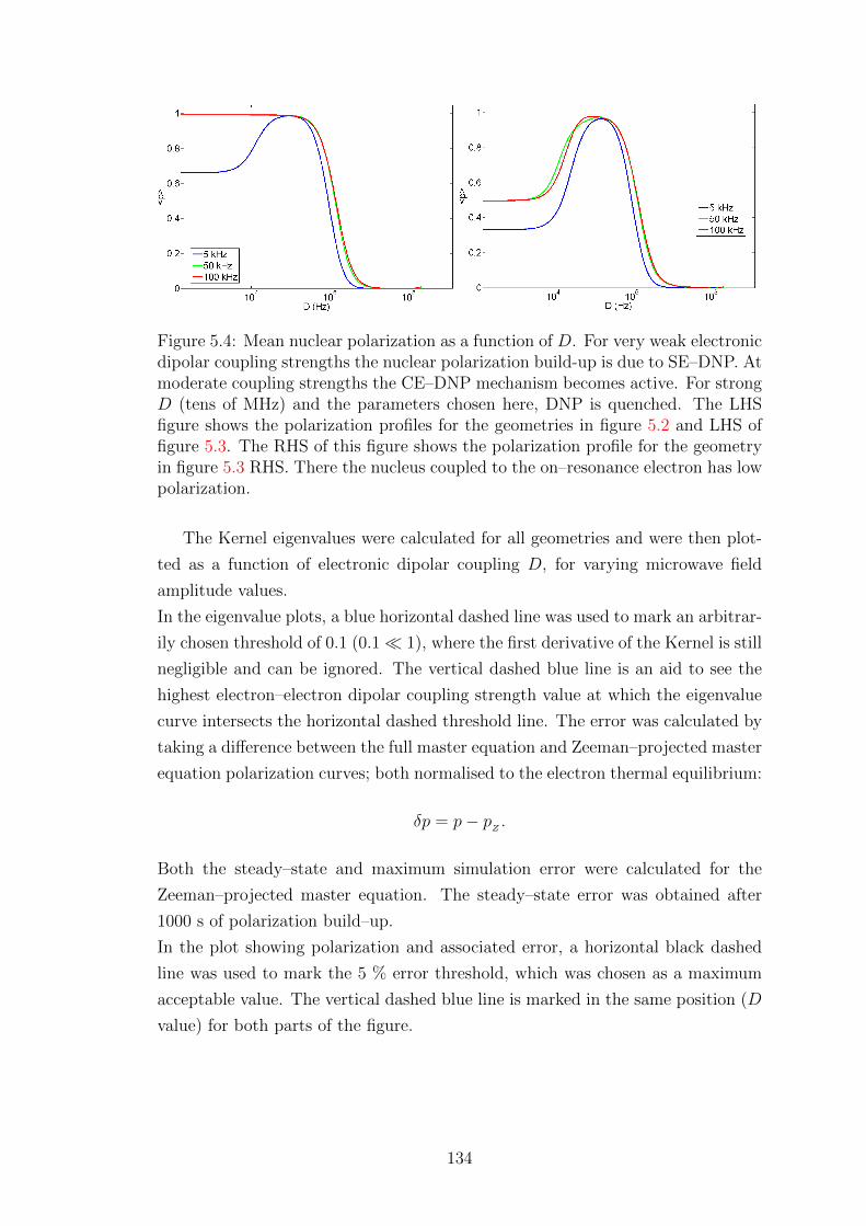
Figure 5.4: Mean nuclear polarization as a function of D. For very weak electronicdipolar coupling strengths the nuclear polarization build-up is due to SE–DNP. Atmoderate coupling strengths the CE–DNP mechanism becomes active. For strongD (tens of MHz) and the parameters chosen here, DNP is quenched. The LHSfigure shows the polarization profiles for the geometries in figure 5.2 and LHS offigure 5.3. The RHS of this figure shows the polarization profile for the geometryin figure 5.3 RHS. There the nucleus coupled to the on–resonance electron has lowpolarization.

The Kernel eigenvalues were calculated for all geometries and were then plot-

ted as a function of electronic dipolar coupling D, for varying microwave field

amplitude values.

In the eigenvalue plots, a blue horizontal dashed line was used to mark an arbitrar-

ily chosen threshold of 0.1 (0.1� 1), where the first derivative of the Kernel is still

negligible and can be ignored. The vertical dashed blue line is an aid to see the

highest electron–electron dipolar coupling strength value at which the eigenvalue

curve intersects the horizontal dashed threshold line. The error was calculated by

taking a difference between the full master equation and Zeeman–projected master

equation polarization curves; both normalised to the electron thermal equilibrium:

δp = p− pZ.

Both the steady–state and maximum simulation error were calculated for the

Zeeman–projected master equation. The steady–state error was obtained after

1000 s of polarization build–up.

In the plot showing polarization and associated error, a horizontal black dashed

line was used to mark the 5 % error threshold, which was chosen as a maximum

acceptable value. The vertical dashed blue line is marked in the same position (D

value) for both parts of the figure.

134

5 kHz

Figure 5.5: Eigenvalues and corresponding error calculated for the geometry infigure 5.2, for ω1 = 5 kHz. The horizontal dashed line is not intersected by theeigenvalue curve, and hence the corresponding error is not excessive - here it isless than 3 %.

Figure 5.6: Eigenvalues and corresponding error calculated for the geometry infigure 5.3 (LHS), for ω1 = 5 kHz. The horizontal dashed line is not intersected bythe eigenvalue curve, and the error does not exceed 1 %.

135

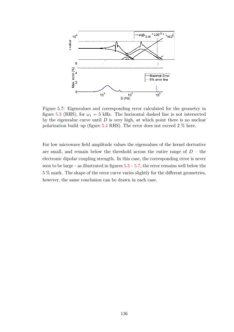
Figure 5.7: Eigenvalues and corresponding error calculated for the geometry infigure 5.3 (RHS), for ω1 = 5 kHz. The horizontal dashed line is not intersectedby the eigenvalue curve until D is very high, at which point there is no nuclearpolarization build–up (figure 5.4 RHS). The error does not exceed 2 % here.

For low microwave field amplitude values the eigenvalues of the kernel derivative

are small, and remain below the threshold across the entire range of D – the

electronic dipolar coupling strength. In this case, the corresponding error is never

seen to be large – as illustrated in figures 5.5 – 5.7, the error remains well below the

5 % mark. The shape of the error curve varies slightly for the different geometries,

however, the same conclusion can be drawn in each case.

136

50 kHz

Figure 5.8: Eigenvalues of the three–part kernel product, and on the bottom theerror between the Zeeman subspace master equation and the full master equation,calculated for the geometry in figure 5.2. Both are plotted as a function of D.The vertical dashed blue line indicates the point where the eigenvalues becometoo large, and where the error can be expected to increase.

Figure 5.9: Eigenvalues of the three–part kernel product, and on the bottom theerror between the Zeeman subspace master equation and the full master equation,calculated for the geometry in figure 5.3 (LHS). Both are plotted as a function ofD. The vertical dashed blue line indicates the point where the eigenvalues becometoo large and thus where the error can be expected to increase.

137

Figure 5.10: Kernel eigenvalues, and the corresponding error between the Zeemansubspace master equation and the full master equation, calculated for the geometryin figure 5.3 (RHS), and shown as a function of D. The vertical dashed blue lineindicates the point where the eigenvalues become too large, and where the errorcan be expected to become large.

It can be clearly seen that the error at ωA = 50 kHz is significant for low–moderate

D values. In this regime the eigenvalues of the first derivative of the Kernel become

too large, resulting in a large error. The error curves vary significantly between the

different geometries, and the maximal error seen in figure 5.9 is slightly lower than

in figure 5.8. It also appears that the range of electron–electron dipolar coupling

strengths for which the error exceeds 5 % is slightly narrower in figure 5.9, yet wider

in figure 5.10. In general, however, it appears that there is a connection between

the eigenvalue magnitude and the corresponding error magnitude in figures 5.8–

5.10.

Figure 5.11: Steady–state error calculated after 1000 s of build–up correspondingfor the geometry in figure 5.2. The microwave field amplitude is 50 kHz. Acomparison to figure 5.8 indicates that at steady–state the error associated withthe projection onto the Zeeman subspace decreases significantly.

138

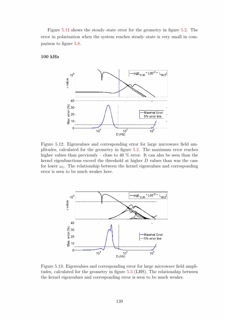
Figure 5.11 shows the steady–state error for the geometry in figure 5.2. The

error in polarization when the system reaches steady–state is very small in com-

parison to figure 5.8.

100 kHz

Figure 5.12: Eigenvalues and corresponding error for large microwave field am-plitudes, calculated for the geometry in figure 5.2. The maximum error reacheshigher values than previously – close to 40 % error. It can also be seen than thekernel eigenfunctions exceed the threshold at higher D values than was the casefor lower ω1. The relationship between the kernel eigenvalues and correspondingerror is seen to be much weaker here.

Figure 5.13: Eigenvalues and corresponding error for large microwave field ampli-tudes, calculated for the geometry in figure 5.3 (LHS). The relationship betweenthe kernel eigenvalues and corresponding error is seen to be much weaker.

139

Figure 5.14: Eigenvalues and corresponding error for large microwave field ampli-tudes, calculated for the geometry in figure 5.3 (RHS).

At high microwave field amplitudes the maximum error increases and remains

excessive for higher D values than was previously the case. In this case there is

also less of a correlation between the error prediction based on eigenvalues, and

the error curve itself.

5.2.3 Summary

Overall it can be seen that there is a link between the eigenvalues of the first

derivative of the kernel function becoming too large to the error seen due to

the projection onto the Zeeman subspace. However, what is more important is

the knowledge of what causes the eigenvalues to become too large. The current

treatment here is indicative but overall not completely sufficient for this purpose,

and a more accurate rigorous, prediction of parameter regions of excessive error

was needed.

In conclusion, finding the point at which the eigenvalues of the kernel triple–

product become too large corresponds relatively well to the region of parameters

where the error between the full master equation and Zeeman–projected master

equation becomes large. Looking at the eigenvalues of the kernel can indicate the

rough value of D, to estimate the boundary beyond which the approximations

required for the Zeeman projection appear to break down.

5.3 Predicting regions of excessive error

The excessive error found for systems with moderate–strength electronic dipolar

coupling (D on the order of 10 kHz – 100 kHz), and where the microwave power is

140

relatively high, has been attributed to one or more of the conditions in eq. (5.10)

being violated. The Hamiltonian terms relevant to the Zeeman projection were

separated in section 5.1.3 between ones that describe the exchange between the

Zeeman and non–Zeeman subspaces; H ′0, H ′1, from the terms that keep dynamics

enclosed in either subspace; H0,0, H1,0.

The Hamiltonian terms H ′0, H′1 when transferred to the Zeeman interaction frame

of reference acquire a time–dependence resulting in an oscillating Hamiltonian

HNZ = ei(H0,0+H1,0)t(H ′0 + H ′1

)e−i(H0,0+H1,0)t,

where it is required that the oscillation frequencies are much higher than the mag-

nitude of the term they are applicable to, thus leading to the strict conditions for

the Zeeman projection eq. (5.10). The conditions of 2–4 in eq. (5.10) are generally

satisfied for parameters typical of CE–DNP. Condition 4 will not be satisfied if the

inter–nuclear separation becomes too small, similarly to the condition in SE–DNP

– eq. (3.15) – relating R(I)2 and |d2

kk′|/4.

The first condition

max(

eig(T0) · eig(Y0))� 1, (5.24)

however, is not satisfied in some cases where the microwave field amplitude ω1 is

significant in comparison to R(S)2 (P 2

0 + (R(S)2 ) 2)−1.

This can be used directly to predict regions where our effective formalism for CE–

DNP will be incorrect, and can be done so quite quickly using numerical analysis

for a system of choice – it does not suffer from the exponential scaling with respect

to the number of spins in a system.

141

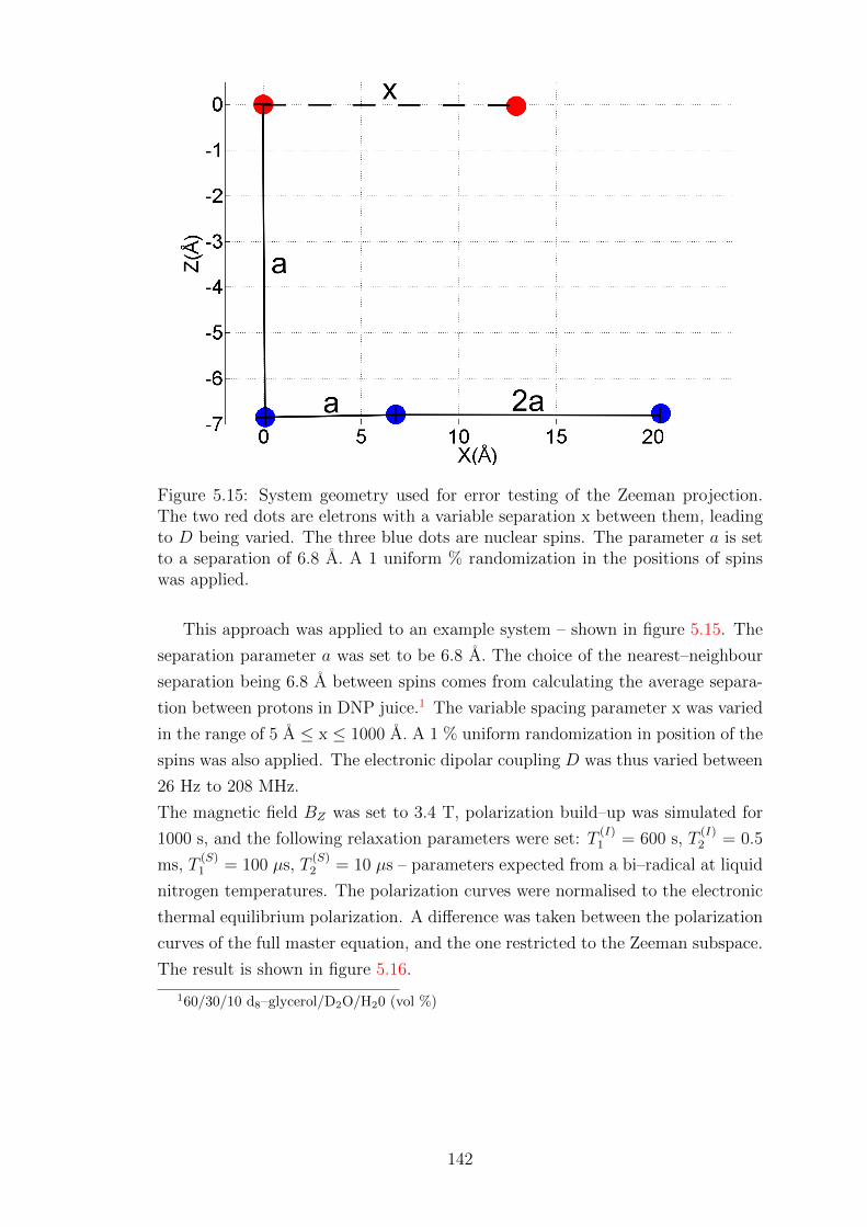
Figure 5.15: System geometry used for error testing of the Zeeman projection.The two red dots are eletrons with a variable separation x between them, leadingto D being varied. The three blue dots are nuclear spins. The parameter a is setto a separation of 6.8 A. A 1 uniform % randomization in the positions of spinswas applied.

This approach was applied to an example system – shown in figure 5.15. The

separation parameter a was set to be 6.8 A. The choice of the nearest–neighbour

separation being 6.8 A between spins comes from calculating the average separa-

tion between protons in DNP juice.1 The variable spacing parameter x was varied

in the range of 5 A ≤ x ≤ 1000 A. A 1 % uniform randomization in position of the

spins was also applied. The electronic dipolar coupling D was thus varied between

26 Hz to 208 MHz.

The magnetic field BZ was set to 3.4 T, polarization build–up was simulated for

1000 s, and the following relaxation parameters were set: T(I)1 = 600 s, T

(I)2 = 0.5

ms, T(S)1 = 100 µs, T

(S)2 = 10 µs – parameters expected from a bi–radical at liquid

nitrogen temperatures. The polarization curves were normalised to the electronic

thermal equilibrium polarization. A difference was taken between the polarization

curves of the full master equation, and the one restricted to the Zeeman subspace.

The result is shown in figure 5.16.

160/30/10 d8–glycerol/D2O/H20 (vol %)

142

Figure 5.16: Zeeman subspace projection error for CE–DNP, shown as a functionof D for several microwave amplitude values. Here a 5 % error has been selectedas an upper limit on the acceptable error. The grey area highlights the range ofD values where for ω1 = 400 kHz the error exceeds the acceptable upper limit.

It can be seen that the error becomes large, and is spread over a greater range

of D for higher microwave field amplitude values, ω1. The area where the error

exceeds 5 % for ω1 = 400 kHz has been shaded in light grey for the purpose of

a visual aid – it covers roughly the range of 10 kHz < D < 1 MHz – and it has

been decided to be outside the acceptable range of accuracy. The region where

the error becomes too large can be predicted using the condition in eq. (5.24).

Figure 5.17 shows the prediction corresponding to figure 5.16, calculated for the

same parameters. The shaded grey region covers the same region in both figures.

The regime where the output of eq. (5.24) increases beyond a certain threshold

(arbitrarily chosen to be 0.1 in this case) indicates the region where the error

will become too large (in figure 5.16). For lower D values the electrons become

decoupled, and SE–DNP is recovered, hence the error decreases again.

143

Figure 5.17: Prediction of regions of excessive error associated with the Zeemanprojection for CE–DNP – predicted using eq. (5.24). The grey area highlightsthe range of D values where for ω1 = 400 kHz the error exceeds 5 %. The figureshows that where the product of |Y0T0| exceeds 0.1 the error becomes excessive.To the left of the shaded area D has low values, and SE–DNP is recovered, thusthe erorr falls again.

Using the above figures it is apparent that even for very high microwave field

amplitudes (ω1 = 400 kHz) our CE–DNP formalism is correct for electronic dipolar

coupling strengths D exceeding 1 MHz. All bi–radicals currently, commonly in use

exceed this coupling strength, meaning the CE–DNP formalism presented here is

suitable for studying such systems. Griffin et al. report in [65] on the coupling

strengths of several bi–radicals. Bi–radicals such as TOTAPOL and BTurea have

D values of 23.2 MHz, and 35.2 MHz respectively; corresponding to separations of

13.1 A and 11.4 A between the electron spins. Even the BTnE (n = 2,3,4) series of

bi–radicals have a coupling strength significantly larger than 1 MHz. Their dipolar

coupling parameters are reported [65] to be 22.2 MHz (BT2E, 13.3 A separation

between electrons), 15.6 MHz (BT3E – 15 A), and 11.6 MHz (BT4E – 16.5 A).

In a previous publication, [66] the same bi–radical family was reported to have D

values of 11 MHz (BT2E), 5.2 MHz (BT3E), and 3.3 MHz (BT4E). These values

still live comfortably outside the region of large error seen in figure 5.16.

5.3.1 Error under shorter decoherence times

The form of the state–dependent rate T0 in eq. (5.14) indicates that the condition

in eq. (5.24) will be satisfied for a greater range of parameters if the decoherence

144

rate is increased, i.e. if T(S)2 is reduced. Figure 5.18 below shows the comparison

to the output from figure 5.16 for T(S)2 reduced from 10 µs to 1 µs.

Figure 5.18: Zeeman subspace projection error for CE–DNP, shown as a functionof D for several microwave amplitude values, T

(S)2 = 1 µs. As before a 5 % error has

been selected as an upper limit on the acceptable error. The grey area highlightsthe range of D values where for ω1 = 400 kHz the error exceeds the acceptableupper limit. With a shorter decoherence time the erorr is reduced for all D values.For microwave field amplitude values of up to 100 kHz the error remains below 5% across the entire range of D.

This is predicted again using the condition in eq. (5.24) for the outlined pa-

rameters, and is shown in figure 5.19. It is very clear that with shorter coherence

times, and low–moderate ω1 values (up to 100 kHz) – the error remains below 5 %

for the entire range of D values. In figure 5.18 is can also be seen that the range

over which the error exceeds 5 % is much more narrow than that which is seen in

figure 5.16.

145

Figure 5.19: Prediction of regions of excessive error associated with the Zeemanprojection for CE–DNP, with T

(S)2 = 1 µs – calculated using eq. (5.24). The grey

area highlights the range of D values where for ω1 = 400 kHz the error exceeds 5%. In this figure the grey region is much more narrow. In addition, |Y0T0| valuesare lower for all ω1.

In order to establish the suitability of using a T(S)2 of 1 µs in simulations, liter-

ature references were compared. Values anywhere in the range of 0.5 µs to 20 µs

are reported. In a theoretical study of transition between SE–DNP and CE–DNP,

the authors in [36] varied T(S)2 between 0.5 µs 20 µs. In [67] an electron T

(S)2 of

10 µs time was set as a ”reasonable guess”. An electronic T(S)2 time of 10 µs is

also reported in [68]. A shorter T(S)2 time of 4 µs was reported by the authors in

[69]. Decoherence time constants of 1 µs were reported in [70, 71], and in [72] the

authors imply a direct measurement of T(S)2 – also to be 1 µs.

Finally, the authors in [73] report measurements of T(S)2 for TOTAPOL and

AMUPol at temperatures of 100 K, and magnetic fields of 3.4 T, 9.8 T. In some

cases bi–exponential fitting was used. For TOTAPOL at 3.4 T the T(S)2 was mea-

sured at 0.1 µs (second time constant – 0.3 µs), and 0.3 µs at 9.8 T.

For AMUPol the corresponding measurements were 0.7 µs and 0.8 µs respectively.

It is worth noting that in some unusual, extreme cases the T(S)2 can be even shorter,

as in the case of silicon nano–particles [74], where the electronic decoherence time

constant can be on the order of tens of nanoseconds.

146

5.3.2 Error testing with shorter T(S)1 times

A study was then conducted relating the electronic longitudinal relaxation time,

T(S)1 to the error seen in the formalism. Figures 5.16 and 5.18 show the error seen

in the formalism for a T(S)1 time of 100 µs. Reducing the T

(S)2 time by one order of

magnitude reduces the error significantly, and it reduces the range over which the

error is excessive. Increasing the electronic T(S)1 relaxation time is seen to reduce

this error further.

Figure 5.20: Zeeman subspace projection error for CE–DNP, shown as a functionof D for several microwave amplitude values and T

(S)2 = 1 µs. Electronic T

(S)1 =

50 ms – top part, and 500 ms for the bottom part. As before a 5 % error has beenselected as an upper limit on the acceptable error. The grey area highlights therange of D values where for ω1 = 400 kHz, and T

(S)1 = 50 ms (top part) the error

exceeds the acceptable upper limit. The grey region is left in the bottom figurefor an easy comparison between the two.

The error in the top part of figure 5.20 is visibly reduced in magnitude for

all ω1 values when T(S)1 is increased to 50 ms. The range over which the error

is excessive is, in addition, reduced in comparison to figure 5.18. Increasing T(S)1

further to 500 ms reduces this error such that for all values of ω1 the maximum

simulation error lies below the 5 % mark.

It is helpful to again relate the parameters used in the simulation to those reported

147

in the literature. The electronic T(S)1 is very temperature dependent. Depending

on the temperature the experiments have been carried out at, the T(S)1 of radicals

and bi–radicals have been reported to be anywhere in the range of 0.1 ms to a few

hundreds of miliseconds. The authors in [70] carried out simulations where T(S)1

times as short as 100 µs were used. In [71] the longitudinal relaxation time is set

to 0.3 ms. One can assume that these values were to correspond to time constants

realistic for samples at 100 K.

In [68] actual T(S)1 measurements were carried out on TEMPOL at temperatures

of 10 K, 20 K and 40 K. The T(S)1 times the authors report are 17 ms, 5.3 ms,

and 0.8 ms respectively. For TEMPOL, again, [67] the measurements at 20 K,

7 K, and 2.7 K yield T(S)2 times of 5.5 ms, 50 ms, and 240 ms. For TOTAPOL,

T(S)1 measurements were carried out in [69]. There the T

(S)1 times are shown for

temperatures of 6 K – 40 K. These are as follows: 40 K: ∼ 1 ms, 30 K: ∼ 1 ms,

20 K: 10 ms, 10 K: 60 ms, and 5 K: 150 ms. In [73] the T(S)1 for TOTAPOL at

100 K was measured to be 10 µs (second fitting constant 50 µs) at 3.4 T, and 9

µs (50 µs for the second time constant) at 9.8 T.

For AMUPol the corresponding time constants were 50 µs (160 µs – second time

constant) at 3.4 T, and 60 µs (230 µs for the second fitting constant) at 9.8 T.

Nuclear longitudinal relaxation times T(I)1 are reported to be anywhere in the range

of seconds to minutes, whereas the transverse relaxation times T(I)2 are anywhere

between 3 µs to 1 ms, in publications [36], [67] – [72].

This shows that the parameters chosen by us for the simulations are reasonable

and are within experimental measurements.

148

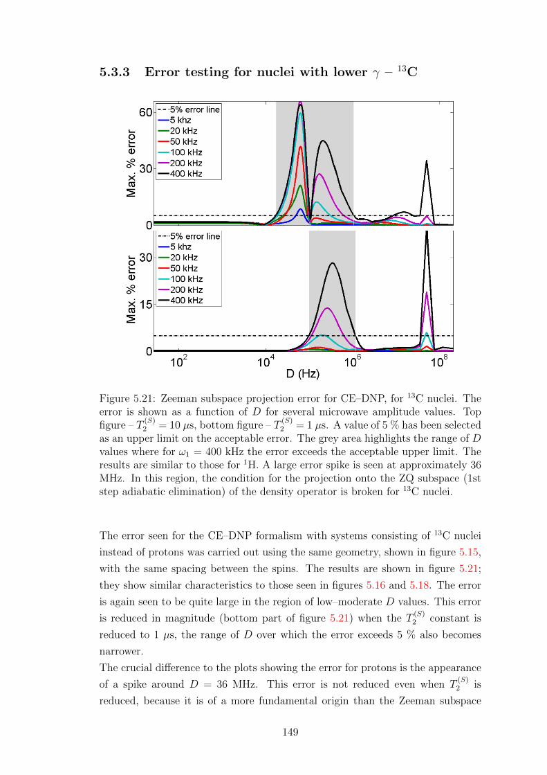
5.3.3 Error testing for nuclei with lower γ – 13C

Figure 5.21: Zeeman subspace projection error for CE–DNP, for 13C nuclei. Theerror is shown as a function of D for several microwave amplitude values. Topfigure – T

(S)2 = 10 µs, bottom figure – T

(S)2 = 1 µs. A value of 5 % has been selected

as an upper limit on the acceptable error. The grey area highlights the range of Dvalues where for ω1 = 400 kHz the error exceeds the acceptable upper limit. Theresults are similar to those for 1H. A large error spike is seen at approximately 36MHz. In this region, the condition for the projection onto the ZQ subspace (1ststep adiabatic elimination) of the density operator is broken for 13C nuclei.

The error seen for the CE–DNP formalism with systems consisting of 13C nuclei

instead of protons was carried out using the same geometry, shown in figure 5.15,

with the same spacing between the spins. The results are shown in figure 5.21;

they show similar characteristics to those seen in figures 5.16 and 5.18. The error

is again seen to be quite large in the region of low–moderate D values. This error

is reduced in magnitude (bottom part of figure 5.21) when the T(S)2 constant is

reduced to 1 µs, the range of D over which the error exceeds 5 % also becomes

narrower.

The crucial difference to the plots showing the error for protons is the appearance

of a spike around D = 36 MHz. This error is not reduced even when T(S)2 is

reduced, because it is of a more fundamental origin than the Zeeman subspace

149

projection. The simulations were carried out at BZ = 3.4 T, meaning the Larmor

frequency ωI of 13C nuclei is approximately 34 MHz. The error spike for high

D values appears due to a violation in the conditions of the projection of the

dynamics into the zero–quantum subspace, shown in eq. (5.4). In order to avoid

this issue, one can either carry out simulations for bi–radicals that do not exceed

this electronic coupling strength, or the simulations could be carried out at a

higher magnetic field, increasing ωI .

5.3.4 Error testing summary

In summary the formalism is correct and suitable for simulations involving bi–

radical molecules. For low–moderate microwave field amplitude values, studies

can be accurately carried out on systems resembling two mono–radicals in close

proximity at the CE–DNP resonance condition – for example at ω1 = 100 kHz,

simulations can be carried out for separations between the electronic spins of ∼40 A or less.

There is a region of parameters corresponding to low–medium electronic coupling

strength D where the error becomes large, and it is shown here that this error is re-

duced if the the electronic decoherence time is set to an experimentally reasonable

and realistic value of of 1 µs. It also helps if the T(S)1 time–constant is increased.

Thus simulations in this range of D values can be carried out for bi–radicals with

a larger distance separating the electron spins, studied at low temperatures –

typically of a few Kelvin, where the T(S)1 times increase very significantly.

5.4 Spin diffusion studies

In order to study spin diffusion in 1–D chains of nuclear spins interacting with

a bi–radical electron spin pair; a treatment similar to that applied in the case

of SE–DNP (section 3.3.1) was implemented. The testing geometry is shown in

figure 5.22.

150

Figure 5.22: Spin chain of 30 13C nuclei (blue dots) next to an electron spin pair(red dots). The nuclear spin chain is at an angle of 45◦ to the magnetic field. Theseparation of the electron spins was set to 40 A, and the separation between thenuclear spins (and the distance between electron 2 and the nearest nucleus) wasset to 5 A. A 5 % uniform randomization was applied to the position of all spins.

As in the case of SE–DNP, the first nucleus – treated and referred to as the core

nucleus – is the effective source of polarization diffusing into the spin chain. The

effective rate corresponding to the inter–nuclear flip–flops driving spin diffusion in

eq. (5.13) shows dependence on the states of both electrons, of which there are a

total of four possible permutations.

For simplicity of the diffusion analysis in the 1–D chain, the four effective dipolar

interaction rates were averaged. The following parameters were used for the simu-

lations: ω1 = 50 kHz, T(S)1 = 14.3 ms, T

(S)2 = 10 µs, T

(I)1 = ∞, T

(I)2 = 100 µs, BZ

= 3.4 T. The electronic spins were set to be separated by 40 A, the inter–nuclear

separations, as well as the distance between the second electron to the core nu-

cleus were set to 5 A. The nuclear spin chain was placed at an angle of 45◦ to BZ .

A uniform, 5 % randomization was applied to the position of each spin. Figure

5.16 shows that the parameters chosen here do not result in a large error and are

reliable.

Figure 5.23 shows the polarization contours in the spin system, as a function of

time and distance from the effective source, thus indicating the spin–diffusion

pathways. A comparison to the early–time contours shows a good fit to the

reflective–boundary solution to the diffusion equation (eq. (3.33)) – discussed

in more detail in section 3.3.1. Unsurprisingly then the mechanism of polarization

transport to the bulk in systems exhibiting CE–DNP is spin diffusion. One of the

assumptions is that rate–limiting step is the transfer of polarization between the

core nucleus to the bulk nuclei. This would imply that the rate of diffusion would

151

be the same for a given system regardless of whether the mechanism of nuclear

polarization build–up is SE–DNP or CE–DNP – which tends to be more efficient.

Figure 5.23: A comparison of polarization contours to solutions to the to thediffusion equation with a reflective boundary (red) and without (black), for thegeometry seen in figure 5.22. An average over 100 000 trajectories was taken. Thepolarization contours correspond to polarization level increments of 8 %. There isa better fit of the reflective boundary solution to the polarization contour in thecase of CE–DNP, than was seen for SE–DNP.

In order to verify this, a comparison was made to SE–DNP. The same system

geometry (figure 5.22) was used with electron 1 (on–resonance to the microwave

radiation) removed. The relaxation parameters and ω1 were left unchanged. The

result is shown in figure 5.24 – top part. The bottom part shows a comparison

between the mean nuclear polarization in the chain during build–up for CE–DNP

and SE–DNP. The polarization diffusion constant calculated in the cases of both

CE–DNP and SE–DNP was the same at a value of 5.39 A2/s. This is expected,

however, a comparison between figures 5.23 and 5.24 shows a significant differ-

ence. The system exhibiting CE–DNP shows a quicker polarization build–up –

particularly in the very early stages. In the bottom part of figure 5.24 it does

however appear that the polarization levels would equalise after a long time; at

steady–state. The polarization contours in figure 5.23 do fit the solution to the

diffusion equation much more closely than in the top part of figure 5.24.

It appears that even though in both cases the exchange between the core and

bulk nuclei is the rate–limiting step and the rates of diffusion are identical, the

152

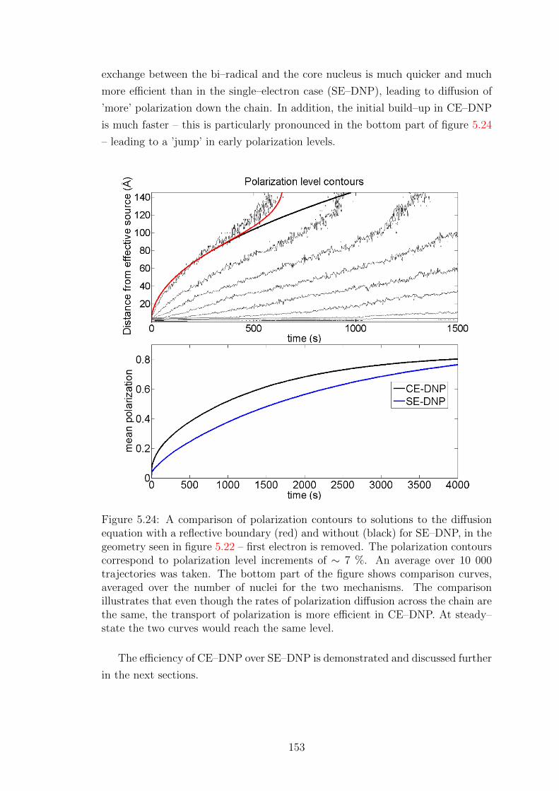
exchange between the bi–radical and the core nucleus is much quicker and much

more efficient than in the single–electron case (SE–DNP), leading to diffusion of

’more’ polarization down the chain. In addition, the initial build–up in CE–DNP

is much faster – this is particularly pronounced in the bottom part of figure 5.24

– leading to a ’jump’ in early polarization levels.

Figure 5.24: A comparison of polarization contours to solutions to the diffusionequation with a reflective boundary (red) and without (black) for SE–DNP, in thegeometry seen in figure 5.22 – first electron is removed. The polarization contourscorrespond to polarization level increments of ∼ 7 %. An average over 10 000trajectories was taken. The bottom part of the figure shows comparison curves,averaged over the number of nuclei for the two mechanisms. The comparisonillustrates that even though the rates of polarization diffusion across the chain arethe same, the transport of polarization is more efficient in CE–DNP. At steady–state the two curves would reach the same level.

The efficiency of CE–DNP over SE–DNP is demonstrated and discussed further

in the next sections.

153

5.5 Optimisation studies

The analytical form of the effective dynamics for CE–DNP in eq. (5.14) provides

a clearer insight into the mechanism that leads to build–up of nuclear polariza-

tion. The form of the rates also provides a hint to the possibility of increasing

the efficiency of the mechanism and making the process more optimised. For the

CE–DNP mechanism to be efficient, the rates corresponding to operators Y0, Y3k

in eq. (5.14) should be as large as possible. The rate corresponding to Y0 de-

scribes the process of saturation of the on–resonance electron, whereas the rate

corresponding to Y3k describes the three–spin flip processes characteristic of the

CE–DNP mechanism.

The state dependent coefficients P0, P3k reduce the magnitude of the respective

rates. The presence of the offset terms λ1, and λ2 in the respective coefficients

points to a possibility of ’tuning’ and reducing the magnitude of operators P0,

P3k. The parameter P0 depends on ωI , D, A(1)k , and bk1, which in turn depends

on B(1)k±, B

(2)k±. The secular and pseudo–secular coupling coefficients are geometry–

dependent and thus vary between spins. The nuclear Larmor frequency and the

electronic dipolar coupling are constants in the model spin systems, thus the mag-

nitude of P0 can be reduced by setting λ1 to λ1 = −D + D2

4ωI.

The coefficients P3k depend on ω1, ωI , D, A(1)k , A

(2)k , bk0, bk1. The last two –

bk0, bk1 depend on the pseudo–secular coupling of a nucleus to the electron spins.

Again, the secular and pseudo–secular couplings are dependent on the geometry

and thus will vary between spins. The parameters ωI , ω1, D are constants in our

spin systems, thus the magnitude of P3k is reduced by setting λ2 = −ω21+D2

2ω1.

Going back to the definition of λ2 (λ2 = ∆2−∆1−ωI), this would imply that the

exact CE–DNP resonance condition is

∆2 −∆1 = ωI −ω2

1 +D2

ω2I

.

In practice, it is likely that this exact resonance condition will be nearly impossible

to target because of the dependence on ω1 which will vary between experiments

and experimental set–ups, and because of the fact that in experiments it is likely

that – due to a distribution of orientations of bi–radicals – D will also vary.

What also follows is that the first electron should be irradiated at

∆1 = −D +D2

4ωI,

and not directly on–resonance with the microwave radiation. This is much more

realistic to achieve experimentally.

This was verified using the Zeeman master equation, eq. (5.16) for a range of

154

λ1, λ2, where −35 MHz ≤ λ1, λ2 ≤ 35 MHz. The test was carried out for the

geometry shown in figure 5.15, with the separation between electron spins set

to 13.1 A (corresponding roughly to the separation in TOTAPOL). With the

vector combining the electron spins being perpendicular to BZ , the D value was

approximately 11.6 MHz. One percent randomization in the position of all spins

was applied, and the following parameters were used: ω1 = 400 kHz, BZ = 3.4 T,

T(S)1 = 100 µs, T

(S)2 = 10 µs, T

(I)1 = 10 mins., T

(I)2 = 0.5 ms. Polarization build–up

was simulated for 1000 s. The result is shown in figure 5.25. It can be seen that

the optimal value for λ1 is just under -10 MHz. Given D ∼ 11.6 MHz, this would

confirm that in fact λ1 = −D + D2

4ωI.

Figure 5.25: Mean steady–state nuclear polarization as a function of frequencyoffsets from the CE–DNP resonance condition; λ1 and λ2. Nuclear polarizationis normalised to the electronic thermal equilibrium polarization. The colour barscale shows the corresponding polarization level. The insert shows the estimatedpolarization build–up time as a function of the same offsets. The calculation wascarried out using the Zeeman–projected master equation. Offsets λ1, λ2 are variedin steps of 0.67 MHz.

The result is less obvious for λ2 where the optimal point lies close to 0. Nu-

merically evaluated for this simulation, the value of λ2 = −ω21+D2

2ω1is ≈ -0.47 MHz,

which would be difficult to see with the resolution of figure 5.25. This result was

then compared to the output seen from the full master equation (eq. (5.2)) using

the same parameters, in order to verify the accuracy. The result is seen in figure

5.26. Using the definitions of offsets λ1, λ2, it is clear to see that figure 5.26 shows

the same results as figure 5.25, on a different grid. There is a transformation of

155

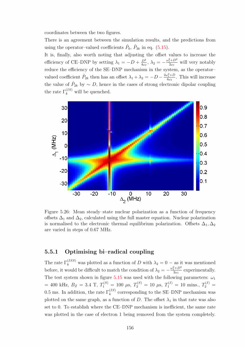
coordinates between the two figures.

There is an agreement between the simulation results, and the predictions from

using the operator–valued coefficients P0, P3k in eq. (5.15).

It is, finally, also worth noting that adjusting the offset values to increase the

efficiency of CE–DNP by setting λ1 = −D + D2

4ωI, λ2 = −ω2

1+D2

2ω1will very notably

reduce the efficiency of the SE–DNP mechanism in the system, as the operator–

valued coefficient P2k then has an offset λ1 +λ2 = −D− 2ω21+D

4ωI. This will increase

the value of P2k by ∼ D, hence in the cases of strong electronic dipolar coupling

the rate Γ(IS)k will be quenched.

Figure 5.26: Mean steady–state nuclear polarization as a function of frequencyoffsets ∆1 and ∆2, calculated using the full master equation. Nuclear polarizationis normalised to the electronic thermal equilibrium polarization. Offsets ∆1,∆2

are varied in steps of 0.67 MHz.

5.5.1 Optimising bi–radical coupling

The rate Γ(ISS)k was plotted as a function of D with λ2 = 0 − as it was mentioned

before, it would be difficult to match the condition of λ2 = −ω21+D2

2ω1experimentally.

The test system shown in figure 5.15 was used with the following parameters: ω1

= 400 kHz, BZ = 3.4 T, T(S)1 = 100 µs, T

(S)2 = 10 µs, T

(I)1 = 10 mins., T

(I)2 =

0.5 ms. In addition, the rate Γ(IS)k corresponding to the SE–DNP mechanism was

plotted on the same graph, as a function of D. The offset λ1 in that rate was also

set to 0. To establish where the CE–DNP mechanism is inefficient, the same rate

was plotted in the case of electron 1 being removed from the system completely.

156

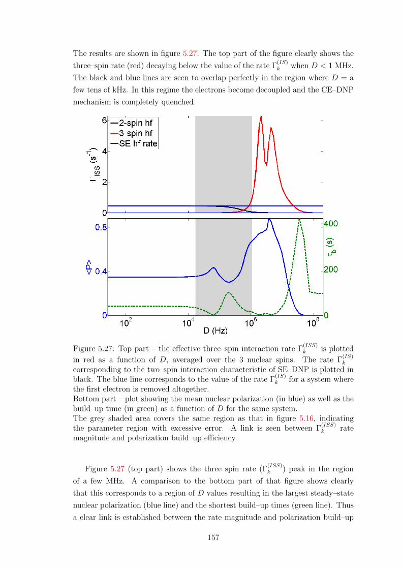
The results are shown in figure 5.27. The top part of the figure clearly shows the

three–spin rate (red) decaying below the value of the rate Γ(IS)k when D < 1 MHz.

The black and blue lines are seen to overlap perfectly in the region where D = a

few tens of kHz. In this regime the electrons become decoupled and the CE–DNP

mechanism is completely quenched.

Figure 5.27: Top part – the effective three–spin interaction rate Γ(ISS)k is plotted

in red as a function of D, averaged over the 3 nuclear spins. The rate Γ(IS)k

corresponding to the two–spin interaction characteristic of SE–DNP is plotted inblack. The blue line corresponds to the value of the rate Γ

(IS)k for a system where

the first electron is removed altogether.Bottom part – plot showing the mean nuclear polarization (in blue) as well as thebuild–up time (in green) as a function of D for the same system.The grey shaded area covers the same region as that in figure 5.16, indicatingthe parameter region with excessive error. A link is seen between Γ

(ISS)k rate

magnitude and polarization build–up efficiency.

Figure 5.27 (top part) shows the three spin rate (Γ(ISS)k ) peak in the region

of a few MHz. A comparison to the bottom part of that figure shows clearly

that this corresponds to a region of D values resulting in the largest steady–state

nuclear polarization (blue line) and the shortest build–up times (green line). Thus

a clear link is established between the rate magnitude and polarization build–up

157

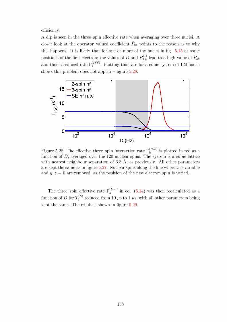
efficiency.

A dip is seen in the three–spin effective rate when averaging over three nuclei. A

closer look at the operator–valued coefficient P3k points to the reason as to why

this happens. It is likely that for one or more of the nuclei in fig. 5.15 at some

positions of the first electron; the values of D and B(1)k± lead to a high value of P3k

and thus a reduced rate Γ(ISS)k . Plotting this rate for a cubic system of 120 nuclei

shows this problem does not appear – figure 5.28.

Figure 5.28: The effective three–spin interaction rate Γ(ISS)k is plotted in red as a

function of D, averaged over the 120 nuclear spins. The system is a cubic latticewith nearest neighbour separation of 6.8 A, as previously. All other parametersare kept the same as in figure 5.27. Nuclear spins along the line where x is variableand y, z = 0 are removed, as the position of the first electron spin is varied.

The three–spin effective rate Γ(ISS)k in eq. (5.14) was then recalculated as a

function of D for T(S)2 reduced from 10 µs to 1 µs, with all other parameters being

kept the same. The result is shown in figure 5.29.

158

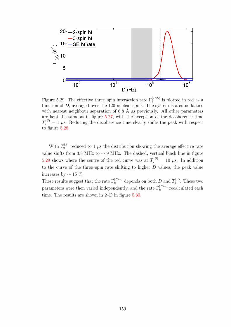
Figure 5.29: The effective three–spin interaction rate Γ(ISS)k is plotted in red as a

function of D, averaged over the 120 nuclear spins. The system is a cubic latticewith nearest neighbour separation of 6.8 A as previously. All other parametersare kept the same as in figure 5.27, with the exception of the decoherence timeT

(S)2 = 1 µs. Reducing the decoherence time clearly shifts the peak with respect

to figure 5.28.

With T(S)2 reduced to 1 µs the distribution showing the average effective rate

value shifts from 3.8 MHz to ∼ 9 MHz. The dashed, vertical black line in figure

5.29 shows where the centre of the red curve was at T(S)2 = 10 µs. In addition

to the curve of the three–spin rate shifting to higher D values, the peak value

increases by ∼ 15 %.

These results suggest that the rate Γ(ISS)k depends on both D and T

(S)2 . These two

parameters were then varied independently, and the rate Γ(ISS)k recalculated each

time. The results are shown in 2–D in figure 5.30.

159

Figure 5.30: The effective three–spin interaction rate Γ(ISS)k is mapped as a func-

tion of D, and R(S)2 averaged over the 120 nuclear spins. The grey–scale bar shows

the magnitude of the rate Γ(ISS)k for a particular set of D and R

(S)2 values. The

insert shows the steady–state polarization (blue) and build–up time (green) as a

function of R(S)1 – the T

(S)1 inverse. Due to the restriction of using a master equa-

tion, the system geometry in figure 5.15 was used for the insert calculation. AT

(S)2 value of 10 µs was used for this calculation, ω1 = 100 kHz, and D = 3.8 MHz.

The figure shows that for increasing D coupling strengths a shorter decoherencetime is also required, and there exists an optimal T

(S)1 for highest polarization.

A very clear dependence on both the transverse relaxation rate R(S)2 and the

electronic dipolar coupling D is seen. For stronger dipolar coupling D there is

a corresponding optimal R(S)2 value, that will maximise the value of the effective

rate Γ(ISS)k . The insert also hints at the existence of an optimal R

(S)1 value for

which the steady–state polarization of the system will be greatest. Given the

result of the comparison in figure 5.27 it can thus be expected that the efficiency

of the CE–DNP mechanism, seen as an output in nuclear polarization, depends on

the relaxation parameters of the electron spins, and the dipolar coupling between

them.

AMUPol and TOTAPOL [65] are bi–radicals that perform quite well in MAS

CE–DNP experiments, resulting in rapid build–up of polarization leading to large

enhancements. The relaxation parameters measured for those bi–radicals in [73]

(written out at the end of section 5.3.2) appear in agreement with the theoretical

160

prediction of figure 5.30. The T(S)1 time measured by the authors lies close to the

peak of the insert in figure 5.30. The T(S)2 values measured by the authors, and the

corresponding D values of those bi–radicals, which are accurately known, place

these bi–radicals along the ’white’ ridge of Γ(ISS)k values of figure 5.30.

It is important to keep in mind that formalism we have developed is applicable to

static samples, the studies of which are currently rather limited [69, 75, 76].

The output seen in figure 5.30 is likely to change with microwave field amplitude,

however it is not expected the difference would be very significant. The trend

with respect to D and T(S)2 is expected to be the same. The insert of figure 5.30

on the other hand is expected to be quite dependent on D, ω1, and T(S)2 , but it

is expected some optimum would exist for a chosen parameter set. The master

equation in eq. (5.16) can be used for a set of desired parameters to determine

the optimal T(S)1 .

Microwave power

Regardless of the fact that the dependency of the efficiency of CE–DNP on the

microwave field amplitude is less severe than that seen in SE–DNP [37], it is

reasonable to expect that there may be some optimal level of microwave power.

To investigate this, several simulations were ran for a cuboid system of 148 1H

spins with a bi–radical embedded within the nuclear spin lattice. The separation

between nearest–neighbour spins was set to 6.8 A, D was set to 3.8 MHz (19 A

separation), T(S)1 = 100 µs, T

(S)2 = 10 µs, T

(I)1 = 10 mins, T

(I)2 = 0.5 ms, BZ =

3.4 T, and a 3 % uniform randomization was applied to the position of the spins.

Simulations were carried out for ω1 values of 5 kHz, 20 kHz, 50 kHz, 100 kHz, 200

kHz, 400 kHz, 700 kHz, and 1000 kHz (the error for which has been verified to

be below 5% at D = 3.8 MHz). A comparison was then made between the mean

nuclear polarization levels reached in each case, after an irradiation of 5 s. Error

bars were established based on the error in the effective formalism, eq. (5.16) at

the value of D = 3.8 MHz. The result is shown in figure 5.31.

161

Figure 5.31: Mean sample polarization as a function of microwave field amplitudeω1, plotted with the estimated error bars. Each point corresponds to the meannuclear polarization after 5 seconds of build–up, for a given microwave field am-plitude. The black, dashed line shows a linear fit to the last three data pointsbased on their scatter.

A line of best fit is also plotted for the last three points in order to take into

account the larger magnitude of error that is seen for these points. The optimal

point of microwave power appears to be around ω1 = 400 kHz, after that the

polarization levels drop.

5.5.2 Simulations for bi–radicals with optimised parame-

ters

Having determined a set of optimal parameters, a large spin simulation was im-

plemented. The system of choice was the same cuboid (5×6×5) with 148 nuclear

spins surrounding a pair of electronic spins. The separation between nearest–

neighbour nuclear spins was 6.8 A, D was set to 3.8 MHz (19 A separation), T(S)1

= 100 µs, T(S)2 = 10 µs, T

(I)1 = 10 mins, T

(I)2 = 0.5 ms, BZ = 3.4 T, and a 3 %

uniform randomization was applied to the position of the spins. The resonance

offset terms λ1, λ2 have been set to their optimal values, determined previously.

The microwave field amplitude was, however, dropped to ω1 = 100 kHz, as this

reduced the computational time by a factor of ∼16. Figure 5.31 shows that a drop

in ω1 from 400 kHz to 100 kHz reduces the polarization level by 33 %, implying

the build–up time has not been severely increased. The polarization build–up of

162

individual spins, in time is shown in figure 5.32.

Figure 5.32: Time–shots showing the build–up of polarization in the cuboid systemwith optimised parameters. The diameter and colour of the spheres indicates thenuclear polarization value for each spin – the scale of which is shown on thecolour bar. The black dots represent the electron spins. A very rapid build–up ofpolarization is seen. After 15 s the average nuclear polarization is 90 % and thespins are close to steady–state.

A rapid build–up of polarization is seen in the spin system, with most nuclei

reaching ∼ 90 % polarization after 15 seconds of irradiation. Nuclei in–plane with

the electron spin pair; i.e. the plane where the coordinate Z ≈ 0, reach lower levels

of polarization in comparison to the remainder of the system. Particularly the

nuclei closest to either electron spin or those in–between the electron spins. These

nuclei are shifted in frequency (an effect analogous to what has been described

in section 4.3) due to the very strong secular coupling to the electronic spins,

and thus the mechanism (corresponding to rates Γ(ISS)k , Γ

(IS)k ) of polarization

transfer for these nuclei is less effective. The mechanism of CE–DNP was directly

compared here to the mechanism of SE–DNP. The first electron spin was moved

163

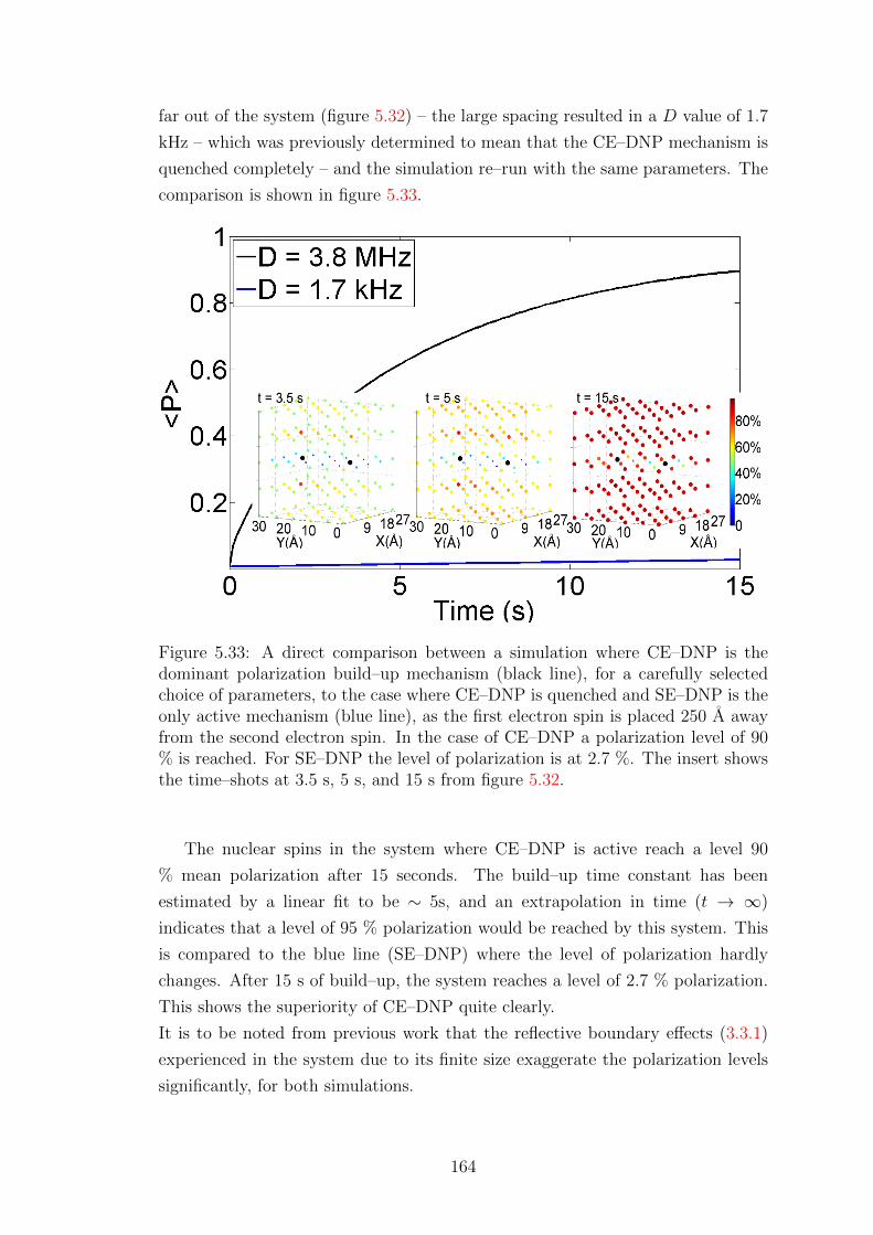
far out of the system (figure 5.32) – the large spacing resulted in a D value of 1.7

kHz – which was previously determined to mean that the CE–DNP mechanism is

quenched completely – and the simulation re–run with the same parameters. The

comparison is shown in figure 5.33.

Figure 5.33: A direct comparison between a simulation where CE–DNP is thedominant polarization build–up mechanism (black line), for a carefully selectedchoice of parameters, to the case where CE–DNP is quenched and SE–DNP is theonly active mechanism (blue line), as the first electron spin is placed 250 A awayfrom the second electron spin. In the case of CE–DNP a polarization level of 90% is reached. For SE–DNP the level of polarization is at 2.7 %. The insert showsthe time–shots at 3.5 s, 5 s, and 15 s from figure 5.32.

The nuclear spins in the system where CE–DNP is active reach a level 90

% mean polarization after 15 seconds. The build–up time constant has been

estimated by a linear fit to be ∼ 5s, and an extrapolation in time (t → ∞)

indicates that a level of 95 % polarization would be reached by this system. This

is compared to the blue line (SE–DNP) where the level of polarization hardly

changes. After 15 s of build–up, the system reaches a level of 2.7 % polarization.

This shows the superiority of CE–DNP quite clearly.

It is to be noted from previous work that the reflective boundary effects (3.3.1)

experienced in the system due to its finite size exaggerate the polarization levels

significantly, for both simulations.

164

5.5.3 CE–DNP at low temperature

It has been shown in this chapter that CE–DNP can be very efficient with the

use of bi–radicals and high microwave power (generally leading to high ω1), what

is important there, as shown in figure 5.30 is that the T(S)1 time should be suf-

ficiently short, so that the first electron is not completely saturated by the mi-

crowave radiation. Thus these experiments are often carried out at relatively high

temperatures (typically 80–100 K) [24]. The longitudinal relaxation times T1 are

dependent on the temperature of the sample, and the magnetic field strength – in

[69] for example the authors take measurements of T(S)1 for TOTAPOL at varying

temperatures.

Figure 5.34: Steady–state polarization and build–up time calculated for the systemgeometry shown in figure 5.15. The parameters are as follows: ω1 = 50 kHz, BZ

= 3.4 T, T(S)2 = 10 µs, T

(I)1 = 10 mins., T

(I)2 = 0.5 ms. The T

(S)1 has been varied

from top to bottom as follows: top part – 100 µs, middle part – 10 ms, bottompart – 100 ms. The shaded area shows the error regime for ω1 = 50 kHz. It canbe seen that with longer T

(S)1 times the peak of the polarization curve shifts to

lower D values, implying that bi–radicals will probably not work well at very lowtemperatures.

165

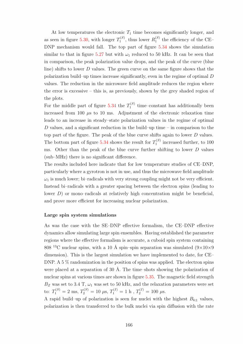
At low temperatures the electronic T1 time becomes significantly longer, and

as seen in figure 5.30, with longer T(S)1 , thus lower R

(S)1 the efficiency of the CE–

DNP mechanism would fall. The top part of figure 5.34 shows the simulation

similar to that in figure 5.27 but with ω1 reduced to 50 kHz. It can be seen that

in comparison, the peak polarization value drops, and the peak of the curve (blue

line) shifts to lower D values. The green curve on the same figure shows that the

polarization build–up times increase significantly, even in the regime of optimal D

values. The reduction in the microwave field amplitude reduces the region where

the error is excessive – this is, as previously, shown by the grey shaded region of

the plots.

For the middle part of figure 5.34 the T(S)1 time–constant has additionally been

increased from 100 µs to 10 ms. Adjustment of the electronic relaxation time

leads to an increase in steady–state polarization values in the regime of optimal

D values, and a significant reduction in the build–up time – in comparison to the

top part of the figure. The peak of the blue curve shifts again to lower D values.

The bottom part of figure 5.34 shows the result for T(S)1 increased further, to 100

ms. Other than the peak of the blue curve further shifting to lower D values

(sub–MHz) there is no significant difference.

The results included here indicate that for low temperature studies of CE–DNP,

particularly where a gyrotron is not in use, and thus the microwave field amplitude

ω1 is much lower; bi–radicals with very strong coupling might not be very efficient.

Instead bi–radicals with a greater spacing between the electron spins (leading to

lower D) or mono–radicals at relatively high concentration might be beneficial,

and prove more efficient for increasing nuclear polarization.

Large spin system simulations

As was the case with the SE–DNP effective formalism, the CE–DNP effective

dynamics allow simulating large spin ensembles. Having established the parameter

regions where the effective formalism is accurate, a cuboid spin system containing

808 13C nuclear spins, with a 10 A spin–spin separation was simulated (9×10×9

dimension). This is the largest simulation we have implemented to date, for CE–

DNP. A 5 % randomization in the position of spins was applied. The electron spins

were placed at a separation of 30 A. The time–shots showing the polarization of

nuclear spins at various times are shown in figure 5.35. The magnetic field strength

BZ was set to 3.4 T, ω1 was set to 50 kHz, and the relaxation parameters were set

to: T(S)1 = 2 ms, T

(S)2 = 10 µs, T

(I)1 = 1 h , T

(I)2 = 100 µs.

A rapid build–up of polarization is seen for nuclei with the highest Bk± values,

polarization is then transferred to the bulk nuclei via spin diffusion with the rate

166

of diffusion along the Z axis significantly (expected to be 2 times greater) faster

than within the X–Y plane; as expected. After 1000 s the core nuclei of the system

are approaching a steady–state, while the polarization of the edge nuclei is slightly

lower. The final mean polarization level of the ensemble is 64 %.

Figure 5.35: A cuboid lattice containing 808 13C spins, surrounding a bi–radicalelectron spin pair. The separation between the electron spins (black dots) is 30A, leading to D of ∼ 0.5 MHz. The nearest–neighbour separation between spinsis 10 A, with a 5 % randomization in the position of each spin. The polarizationlevels of each nuclear spin are shown at times of 10 s, 100 s, 500 s, and 1000 s.Microwave irradiation was simulated for a time of 2000 s. The total simulationrun–time was 36 days on a dual–processor Intel Xeon E5 2690 workstation.

Low temperature comparison between CE–DNP and SE–DNP

A similar system to that shown in figure 5.35 was used to make a comparison

between the mechanisms of SE–DNP and CE–DNP at low temperatures for large

spin ensembles. A symmetric cube was chosen (9×9×9 dimension) as this is

preferred for SE–DNP simulations where the single electron spin is placed in the

167

centre of the system. To keep the symmetry for the equivalent CE–DNP system,

the electron spins were placed at a separation of 40 A, lowering D to 100 kHz. Such

a system could correspond to a pair of mono–radical molecules whose electron spins

are at the CE–DNP resonance condition (∆2 −∆1 ≈ ±ωI), due to a difference in

their magnetic environment. The T(S)1 was increased to 11 ms. The microwave field

amplitude was set to ω1 = 100 kHz for the system exhibiting SE–DNP (for higher

efficiency), for the system with two electron spins it was left unchanged at ω1 =

50 kHz. In both systems, the nuclear–nuclear dipolar interaction was removed

by setting the rates Γ(II)kk′ (eqs. (5.14), (3.25)) to 0. This was done to ignore

spin–diffusion effects and directly compare the efficiency with which polarization

is transferred directly from the electron spins to the surrounding nuclei.

Figure 5.36: Comparison between SE–DNP and CE–DNP for the same systemgeometry. There are no nuclear interactions present in the system. The blackdots denote electronic spins. The microwave field amplitude used in the SE–DNPsimulation is twice as large as that in the case of CE–DNP, otherwise all parametersare identical. The colour bar shows the level of polarization each nucleus has at theend of the simulation. The same scale is used for both parts of the figure. With nopolarization diffusion in the system, the figure illustrates that the effective rangeof interaction between the electrons and nuclei is significantly greater in CE–DNP.

The result is shown in figure 5.36. The figure shows a significant build–up of

nuclear polarization for nuclei with relatively large Bk± values. Other remaining

nuclei show no polarization – as would be expected with no spin diffusion in the

system. Selecting an arbitrary nuclear polarization level, and comparing the dis-

tance at which that level of polarization is found in each system; it was determined

that the range of effective interaction between electrons and nuclei is greater for

CE–DNP by at least a factor of√

2.

168

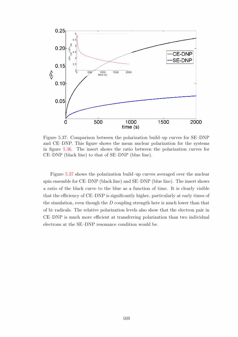
Figure 5.37: Comparison between the polarization build–up curves for SE–DNPand CE–DNP. This figure shows the mean nuclear polarization for the systemsin figure 5.36. The insert shows the ratio between the polarization curves forCE–DNP (black line) to that of SE–DNP (blue line).

Figure 5.37 shows the polarization build–up curves averaged over the nuclear

spin ensemble for CE–DNP (black line) and SE–DNP (blue line). The insert shows

a ratio of the black curve to the blue as a function of time. It is clearly visible

that the efficiency of CE–DNP is significantly higher, particularly at early times of

the simulation, even though the D coupling strength here is much lower than that

of bi–radicals. The relative polarization levels also show that the electron pair in

CE–DNP is much more efficient at transferring polarization than two individual

electrons at the SE–DNP resonance condition would be.

169

Chapter 6

Conclusion & Outlook

A new formalism was developed for SE–DNP and CE–DNP allowing large spin

system simulations. This was carried out by projecting the dynamics of the Liou-

ville von Neumann equation onto the diagonal of the density operator, with the

use of adiabatic elimination and Nakajima–Zwanzig projection operators. The

resulting, effective dynamics are incoherent and were written in the form of Lind-

bladian dissipators. This reduced the dimension of the dynamics from 4n to 2n for

n spins. In addition the form of the effective dynamics allows the use of kinetic

Monte Carlo algorithms, which avoid the exponential growth of the Liouville space

with respect to an increasing number of spins. This permitted simulations of very

large spin systems. The analytical form of the extracted effective rates provides

a clear insight into the mechanism underlying SE–DNP and CE–DNP; a much

clearer understanding than can be obtained from the full quantum–mechanical

formalism.

A comprehensive error analysis was first carried out. We showed that our formal-

ism is accurate for spin–spin separations down to 2 A.

Although the formalism is accurate over a wide range of parameters, there are real

systems where it is not suitable. One example of a system that cannot be mod-

elled using the effective dynamics is a sample of silicon micro/nano – particles [74],

[77]. Given the high concentration of electron radicals these samples may contain,

it is questionable whether the SE–DNP mechanism is the dominant DNP mech-

anism, and whether the full Liouvillian in eq. (3.2) would be suitable to start with.

In our formalism the entire dynamics of SE–DNP are described using four rates,

one of which is state–dependent. The rates described correspond to particular

operations in the system e.g. single spin flips describing relaxation, and flip–flops

describing polarization exchange between spins in the system. Simulating large

linear spin systems we have found the mechanism of polarization transport to the

bulk in DNP to be spin diffusion. We have simulated the polarization dynamics

170

in very large spin ensembles and demonstrated a possibility of fitting polarization

curves of individual spins, in order to reduce the polarization error and the num-

ber of kMC trajectories executed in the simulation. We have shown the scaling of

the random error associated with Monte Carlo algorithms, as well as the simula-

tion run–time with respect to an increasing number of spins. In addition we have

demonstrated how the projection onto the Zeeman subspace can be extended to

heteronuclear systems, with nuclei close in Larmor frequency values. Finally for

SE–DNP, we have found a formalism suitable for nuclei with lower γ values (e.g.13C) that relies on linear rates, avoiding kMC algorithms and quantum master

equations, allowing one to simulate spin systems of tens of thousands of spins in

a matter of minutes.

In chapter 4 the necessity and clear advantage of using large spin system simula-

tions, when studying the mechanism of DNP, were shown. A study was conducted,

analysing the effect of nuclei in immediate vicinity to the electron, on DNP perfor-

mance – in terms of transport of polarization to the bulk. We studied the effect of

the removal of core nuclei on polarization build–up rates of the remaining nuclei

as well as their steady–state ensemble polarization values. A clear improvement

in both can be seen when core nuclei – those in the immediate vicinity of the

electron, are removed from the system. Build–up rates increase significantly, and

the mean steady–state polarization level increases by more than a factor of 2. We

have explained this using simulated DNP transition spectra, which illustrate the

effect of linewidth narrowing with the removal of nuclei strongly coupled to the

electron. The rate of spin–diffusion into the bulk is also significantly improved

with the removal of core nuclei. Crucially, the improvement can be explained us-

ing the effective rates. The results presented here may give an insight or guidance

in radical–design for optimised DNP experiments. The efficiency of designed rad-

icals can be theoretically predicted and assessed.

Chapter 5 focuses on the effective dynamics of CE–DNP, obtained by adia-

batic elimination. The entire dynamics of CE–DNP are described using seven

rates, most of which are state dependent. As was the case with SE–DNP, the

mechanism of polarization transport to the bulk was determined to be spin diffu-

sion. A comprehensive error analysis was carried out and we have demonstrated

that regions of excessive error can be predicted quite accurately. The formalism

is suitable for simulating dynamics of systems containing bi–radicals or mono–

radicals in close proximity – found at the CE–DNP resonance condition. The

analytical form of the effective rates provides a clear insight into the mechanism

underlying CE–DNP. A link is found between the magnitude of the three–spin

rate, and the magnitude of the steady–state polarization and nuclear polarization

171

build–up time. The dependence of polarization on microwave power and electronic

T1 times is shown. A crucial dependence of the three–spin rate on the electronic

dipolar coupling strength and decoherence times is also illustrated. The effective

rates thus provide a means of predicting the efficiency of bi–radicals and give some

optimisation capability; the effectiveness of a parameter choice can be studied from

a theoretical point of view before synthesis. Large spin system simulations were

then executed with an improved parameter choice, for bi–radicals, and this was

seen to lead to a very rapid build–up of polarization.

The work presented here is one of many important steps taken to understand DNP,

in order to maximise its effectiveness. We have provided a lot of new insight into

the mechanisms of SE–DNP and CE–DNP for static solid–state samples, through

a new formalism enabling simulations of large spin systems. The limitations of

the formalism are that as it stands, it cannot be used to simulate frequency–sweep

experiments nor MAS DNP. Future work will involve extensions of this formalism

to the case of rotating solids.

It has been recently found that the dynamics of a system containing several elec-

trons and one nuclear spin can be described by a master equation in the Lindblad

form [78]. Work on TM–DNP and an effective formalism describing the dynamics

there would be sought after. A formalism where any or all of the three solid–state

DNP mechanisms are present would also be of interest. Especially since there are

very few experiments published in the literature where SE–DNP seems to be the

sole mechanism for generating non–thermal nuclear spin states.

Fundamental work by Vega and co–workers has demonstrated that a mixture of

SE–DNP and CE–DNP is responsible for the build up of nuclear polarization at

cryo–temperatures using the trityl radical [67, 79]. Even for such complex systems

it appears to be feasible, based on our work involving the reduction of the required

state space, to derive a set of equations that can describe the nuclear polarization

dynamics.

Finally, it would be of interest to study the newly–discovered mechanisms of OE–

DNP found in insulating solids during magic angle spinning, and the promising

concept of pulsed DNP.

172

Appendix

A.1 Commutative form of Hamiltonian superop-

erators

As mentioned in the main text, the double-hat notation implies a commutation

operation, i.e. for some arbitrary operator X; ˆX =[X, ρ

]. The form of superop-

erator M1 may be re-written as follows

M1 = −i[

ˆH+,ˆH−

][

ˆH+,ˆH−

]ρ =

(ˆH+

ˆH− − ˆH−ˆH+

)ρ = ˆH+

(H−ρ− ρH−

)− ˆH−

(H+ρ− ρH+

). . .

= H+H−ρ− H+ρH− − H−ρH+ + ρH−H+

−H−H+ρ+ H−ρH+ + H+ρH− − ρH+H− . . .

=(H+H− − H−H+

)ρ− ρ

(H+H− − H−H+

).

Hence it is clear that

M1 = −i[

ˆH+,ˆH−

]≡ −i ˆH1,

where

H1 =(H+H− − H−H+

)=[H+, H−

].

A.2 Explicit derivation of rate ΓIS for a two-spin

system

The two-spin SE-DNP, Zeeman-subspace Master equation is well approximated

by˙ρZ

=(Γ′ + PZM2PZ − L0,01L11

−1L0,10

)ρZ. (6.1)

173

To find an explicit form of L−100 , one is looking for an operator X that satisfies

L00XH′1ρZ = H ′1ρZ .

Given H ′1 = − ω1

4ωI

(B+I+S− +B−I−S+

), we can define the operator Y = B+I+S−

for convenience. Its Hermitian conjugate is Y † = B−I−S+. With the lack of

dipolar interactions in a system of one nucleus;

L0,10 = QCH ′1PZ = H ′1, L0,01 = PZH ′1QC = H ′1.

The right-hand size of eq. (6.1) is derived as follows

L0,01L11−1L0,10 ρZ =

ω1

4ωI

(ˆY + ˆY †

)L−100

ω1

4ωI

(ˆY + ˆY †

)ρZ. . .

=ω2

1

16ω2I

(ˆY + ˆY †

)L−100

(ˆY ρ

Z+ ˆY †ρ

Z

). . .

=ω2A

16ω2I

(ˆY + ˆY †

)((R12 + iD

)−1 ˆY ρZ

+(R12 − iD

)−1 ˆY †ρZ

).

Here R12 = (R(S)2 +R

(I)2 ) and D = λ+

ω21

2ωI− |B±|

2

8ωI. Both

(R12 ± iD

)−1

commute

with Y and Y †, and ˆY ˆY ρZ

= 0 as well as ˆY † ˆY †ρZ

= 0. Thus,

LZ,00

L00−1L

00,ZρZ

=ω2

1

16ω2I

((R12 + iD

)−1 ˆY † ˆY ρZ

+(R12 − iD

)−1 ˆY ˆY †ρZ

). . .

=ω2A

16ω2I

((R12 + iD

)−1 (Y †Y ρ

Z− Y †ρ

ZY − Y ρ

ZY † + ρ

ZY Y †

)+(

R12 − iD)−1 (

Y Y †ρZ− Y ρ

ZY † − Y †ρ

ZY + ρ

ZY †Y

)ρZ

).

Because[ρZ, Y Y †

]= 0,

[ρZ, Y †Y

]= 0

LZ,00

L00−1L

00,ZρZ

= . . .

− ω21

16ω2I

((R12 + iD

)−1

+(R12 − iD

)−1)(

Y ρZY † − 1

2

{ρZ, Y †Y

}). . .

− ω21

16ω2I

((R12 + iD

)−1

+(R12 − iD

)−1)(

Y †ρZY − 1

2

{ρZ, Y Y †

}).

174

Since(R12 + iD

)−1

+(R12 − iD

)−1

=R12 − iDR12

2 + D2+

R12 + iD

R122 + D2

=2R12

R122 + D2

,

LZ,00

L00−1L

00,Zρ

Z= − ω2

1

8ω2I

R12

R122 + D

2

(D[Y ] + D[Y †]

)ρZ.

The complex coefficients B± can be factored out, by taking out the absolute value

|B±|, allowing the operator Y to be re-written as Y = I+S−, and hence the

nuclear-electronic flip-flop dissipator becomes

Γ(IS)1 =

ω21 |B±|

2

8ω2I

R12

R122 + D2

(D[Y ] + D[Y †]

), (6.2)

where as before Y = I+S−, R12 = R(S)2 +R

(I)2 , and D = λ+

ω2A

2ωI− |B±|

2

8ωI.

A.3 Computational form of operator-valued rates

For an arbitrary Hermitian operator Sα, acting on an arbitrary density operator

ρ;

Sα =

(α γ

γ∗ β

); ρ =

(a c

c∗ b

)where {a, b, c, α, β, γ} ∈ C; the column density matrix can be written in column-

stacked form

col ρ =

a

c∗

c

b

. (6.3)

The following is true in general:

col

(Sαρ

)=

αa+ γc∗

γ∗a+ βc∗

αc+ γb

γ∗c+ βb

6= col

(ρSα

)=

αa+ γ∗c

αc∗ + γ∗b

γa+ βc

γc∗ + βb

.

A superoperator form, which would give the same result when acting on the

column-stacked density matrix i.e. col ρ in eq. (6.3) is sought after.

One such possibility is(

1⊗ Sα)

which acting on eq. (6.3) gives the following

175

result:

Sα col ρ =(

1⊗ Sα)

col ρ =

α γ 0 0

γ∗ β 0 0

0 0 α γ

0 0 γ∗ β

col ρ =

αa+ γc∗

γ∗a+ βc∗

αc+ γb

γ∗c+ βb

.

The other is(S∗α ⊗ 1

)- here the asterisk represents a matrix conjugate, not to be

mistaken with a Hermitian conjugate.

S′α col ρ =(S∗α ⊗ 1

)col ρ =

α 0 γ∗ 0

0 α 0 γ∗

γ 0 β 0

0 γ 0 β

col ρ =

αa+ γ∗c

αc∗ + γ∗b

γa+ βc

γc∗ + βb

.

From this one can conclude that

Sαρ ≡(

1⊗ Sα)

col ρ

ρSα ≡(

¯Sα ⊗ 1

)col ρ.

This property is generally expected to be true for 2×2 matrix operators, and their

Kronecker products - applicable to spin-1/2 systems.

If an arbitrary operator Sα acts on a Lindbladian dissipator of the form

˙ρ = SαD[Lk]ρ = Sα

(LkρL

†k − 1/2

{ρ, L†kLk

})then if the Lindblad dissipator is re-written to act on a column density operator

col ρ, i.e.

˙col ρ = Sα

(L∗k ⊗ Lk −

1

21⊗ L†kLk −

1

2(L†kLk)

∗ ⊗ 1

)col ρ,

then the superoperator Sα has the form

Sα =(

1⊗ Sα).

176

A.4 Overhauser Effect dynamics projected onto

Zeeman subspace

Solid-state Overhauser Effect DNP (OE-DNP) is most prominent in samples where

the electron radical is delocalised over a relatively large volume. As example

of such systems exhibiting OE-DNP would be metal conductors, graphene and

samples with free radicals. The mechanism relies on the stochastic interactions

between an electron and nuclei, which lead to cross-relaxation flip-flop or flip-flip

transitions of the electron and a nucleus, driven by saturation of the electronic

spin transition. The stochasticity of the interaction between an electron and a

nucleus arises due to rotations and/or vibrations in the lattice. The OE will be

most efficient if in the spectral density spectrum of a sample, there is a large

difference in density values between the frequencies corresponding to ZQ, and DQ

transitions.

More recently OE-DNP has been shown to be present in insulating solids which

are subject to MAS [24]. There the mechanism is advantageous as it appears that

the DNP enhancement increases with an increase in the magnetic field strength.

The system Hamiltonian in the rotating frame of reference can be rewritten for

convenience;

HZ = ∆Sz +∑k

ωI Ikz,

H0 = λSz +ω1

2(S+ + S−) +

∑k

AkSz Ikz

+∑kk′

dkk′(2Ikz Ik′z −1

2Ik+Ik′− −

1

2Ik−Ik′+),

H± =∑k

Bk±Sz Ik±.

The system is also subject to longitudinal relaxation back to thermal equilibrium,

decoherence, and double-quantum as well as zero-quantum cross-relaxation tran-

sitions

Γ = Γ(S)+ D[S+] + Γ

(S)− D[S−] + Γ(S)

z D[Sz] +∑k

(Γ(I)k+D[Ik+] + Γ

(I)k−D[Ik−] + Γ

(I)kz D[Ikz]

+Γ(SI)++ D[T+] + Γ

(SI)−− D[T−] + Γ

(SI)+− D[U+] + Γ

(SI)−+ D[U−]),

where the operators T, U are

T± = S±Ik± U± = S±Ik∓.

177

These are responsible for double-quantum and zero-quantum cross-relaxation tran-

sitions, respectively.

The OE resonance condition is ∆ ≈ 0. At this condition, the Zeeman Hamiltonian

becomes HZ =∑

k ωI Ikz.

As was the case with projections for SE-DNP and CE-DNP, the Liouville state

space can be decomposed as

L =∑Lq,

where Lq is the subspace of q-quantum coherences,

ˆH Z ρ = qωI ρ, ρ ∈ Lq, q = 0, ±1, . . . , ±(n+ 1). (6.4)

Since

ωI � Ak, Bk±, dkk′ ,Γ(S)z ,Γ

(I)kz ,Γ

(S)± ,Γ

(I)k±,Γ

(SI)±± ,Γ

(SI)±∓ ,

dynamics in the subspace where ˆH Z ρ = qωI ρ, for q 6= 0 evolve on a time-scale

much faster than the subspace where ˆH Z ρ = 0. It is thus possible to separate the

dynamics between these subspaces. The Hilbert subspace that commutes with

HZ is referred to from hereon as the zero-quantum subspace. It is in fact the

zero-quantum subspace of the nuclear spins. This projection itself is analogous to

projecting the dynamics onto the subspace of nuclear spins and the off-resonance

electron in the CE-DNP case, as there the first (on-resonance) electron is also

saturated by microwave radiation.

Under the conditions

(2R(I)2 )2 � d 2

kk′

4

(R(S)2 )2 �

{ω2

1

2, R

(S)1 , R

(I)1 ,Γ

(SI)±± ,Γ

(SI)±∓

}(6.5)

using the adiabatic elimination procedure described in section 2.4 it is possible

to project the OE-DNP dynamics onto the Zeeman subspace resulting in effective

classical-like dynamics

˙ρ = LZρ, LZ = L0,00 + M′, M′ = −L0,01L0,11−1L0,10. (6.6)

Here

L0,00 = Γ′ + Γ′′,

178

and the superoperator M′ is well approximated as

M′ =∑k<k′

Γ(II)kk′ D[Xkk′ ]. (6.7)

where Γ′ is

Γ′ = Γ(S)+ D[S+] + Γ

(S)− D[S−] +

∑k

(Γ(I)k+D[Ik+] + Γ

(I)k−D[Ik−]

+Γ(SI)++ D[T+] + Γ

(SI)−− D[T−] + Γ

(SI)+− D[U+] + Γ

(SI)−+ D[U−])

and Γ′′ is

Γ′′ =ω2

1

2

R(S)2

(R(S)2 )2 + α2

(D[S+] + D[S−]

)+|Bk|2R(I)

2

8ω2I

∑k

(D[Ik+] + D[Ik−]

),

and

Γ(II)kk′ =

d2kk′

2

2R(I)2

(2R(I)2 )2 + β 2

kk′

,

Xkk′ = (Ik+Ik′− + Ik−Ik′+),

α = λ1 +∑k

AkIkz,

βkk′ = (Ak − Ak′)Sz +1

8ωI(|Bk|2 − |Bk′|2)1.

(6.8)

As was the case with SE-DNP and CE-DNP, the effective dynamics show a state-

dependence - eq. (6.8). Kinetic Monte Carlo algorithms can be used to simulate

large spin system ensembles.

179

Bibliography

[1] I. Bertini, K.S. McGreevy, and G. Parigi. NMR of Biomolecules. Wiley–

Blackwell, 2012.

[2] K. Wutrich et al. Improved spectral resolution in cosy 1H NMR spectra of

proteins via double quantum filtering. Biochem. Biophys. Res. Commun.,

117(2):497–485, 1983.

[3] S. B. Shuker, P. J. Hajduk, R. P. Meadows, and S. W. Fesik. Discovering

high–affinity ligands for proteins: SAR by NMR. Science, 274(5292):1531–

1534, 1996.

[4] F. Chiti and C. M. Dobson. Protein misfolding, functional amyloid, and

human disease. Annu. Rev. Biochem., 75(1):333–366, 2006.

[5] S. V. Dvinskikh, V. Castro, and D. Sandstrom. Heating caused by radiofre-

quency irradiation and sample rotation in 13 C magic angle spinning NMR

studies of lipid membranes. Magn. Reson. Chem., 42(10):875–881, 2004.

[6] H. J. Jakobsen, A. R. Hove, R. G. Hazell, H. Bildsoe, and J. Skibsted. Solid–

state 14 N MAS NMR of ammonium ions as a spy to structural insights for

ammonium salts. Magn. Reson. Chem., 44(3):348–356, 2006.

[7] J.-L. Hodeau and R. Guinebretiere. Crystallography: past and present. Appl.

Phys. A, 89(4):813–823, 2007.

[8] F. W. Wehrli. On the 2003 nobel prize in medicine or physiology awarded to

Paul C. Lauterbur and Sir Peter Mansfield. Magn. Reson. Med., 51(1):1–3,

2004.

[9] P.M. Matthews et al. Advances in functional and structural MR image analy-

sis and implementation as FSL. NeuroImage, 23, Supplement 1:S208 – S219,

2004.

[10] S. Ogawa, T.M. Lee, and D.W. Tank. Brain magnetic resonance imaging

with contrast dependent on blood oxygentation. Proc. Natl. Acad. Sci.,

87(24):9868–9872, 1990.

180

[11] E. J. Hall and D. J. Brenner. Cancer risks from diagnostic radiology. Brit.

J. Radiol., 81(965):362–378, 2008.

[12] M. H. Levitt. Spin Dynamics. Wiley, 2008.

[13] J. S. Natterer and J. Bargon. Parahydrogen induced polarization. Prog. Nucl.

Mag. Res. SP., 31(4):293 – 315, 1997.

[14] P. Maletinsky et al. A robust scanning diamond sensor for nanoscale imaging

with single nitrogen–vacancy centres. Nature, 7:320–324, 2012.

[15] C. C. Vassiliou et al. Room–temperature in situ nuclear spin hyperpolar-

ization from optically pumped nitrogen vacancy centres in diamond. Nat.

Commun., 6:8965, 2015.

[16] T. G. Walker and W. Happer. Spin–exchange optical pumping of noble–gas

nuclei. Rev. Mod. Phys., 69:629–642, Apr 1997.

[17] J. F. G. Vliegenthart et al. Carbohydrate–protein interaction studies by laser

photo CIDNP NMR methods. Glycoconjugate J., 14(4):531–534, 1997.

[18] D. C. Williamson et al. Reversible interactions with para–hydrogen enhance

nmr sensitivity by polarization transfer. Science, 323(5922):1708–1711, 2009.

[19] L. C. L. Hollenberg et al. The nitrogen–vacancy colour centre in diamond.

Phys. Rep., 528(1):1 – 45, 2013.

[20] J. Wrachtrup et al. Dynamic polarization of single nuclear spins by optical

pumping of nitrogen–vacancy color centers in diamond at room temperature.

Phys. Rev. Lett., 102:057403, Feb 2009.

[21] H.R. Ward. Chemically induced dynamic nuclear polarization (CIDNP). I.

Phenomenon, examples, and applications. Acc. Chem. Res., 5(1):18–24, 1972.

[22] S. H. Pine. Chemically induced dynamic nuclear polarization. J. Chem.

Educ., 49(10):664, 1972.

[23] J. E. Harriman. Theoretical Foundations of Electron Spin Resonance, vol-

ume 37. Academic Press, 1978.

[24] T.V. Can, Q.Z. Ni, and R.G. Griffin. Mechanisms of dynamic nuclear polar-

ization in insulating solids. J. Magn. Reson., 253:23 – 35, 2015.

[25] R. G. Griffin and T. F. Prisner. High field dynamic nuclear polarization–the

renaissance. Phys. Chem. Chem. Phys., 12:5737–5740, 2010.

181

[26] T. Maly et al. Dynamic nuclear polarization at high magnetic fields. J. Chem.

Phys., 128(5), 2008.

[27] K. M. Brindle et al. Detecting tumor response to treatment using hyperpolar-

ized 13C magnetic resonance imaging and spectroscopy. Nat. Med., 13:1382–

1387, 2007.

[28] J. A. Murray et al. Metabolic imaging of patients with prostate cancer using

hyperpolarized 1–13C pyruviate. Science Trans. Med., 5:198ra108, 2013.

[29] K. Golman et al. Increase in signal–to–noise ratio of > 10,000 times in liquid-

state NMR. Proc. Natl. Acad. Sci., 100(18):10158–10163, 2003.

[30] C.-G. Joo, K.-N. Hu, J. A. Bryant, and R. G. Griffin. In situ temper-

ature jump high–frequency dynamic nuclear polarization experiments: en-

hanced sensitivity in liquid–state NMR spectroscopy. J. Am. Chem. Soc.,

128(29):9428–9432, 2006.

[31] A. W. Overhauser. Polarization of nuclei in metals. Phys. Rev., 92:411–415,

Oct 1953.

[32] T. R. Carver and C. P. Slichter. Experimental verification of the overhauser

nuclear polarization effect. Phys. Rev., 102:975–980, May 1956.

[33] A. K. Geim and K. S. Novoselov. The rise of graphene. Nat. Mat., 6:183–191,

2007.

[34] Y. Hovav, A. Feintuch, and S. Vega. Theoretical aspects of dynamic nuclear

polarization in the solid state – spin temperature and thermal mixing. Phys.

Chem. Chem. Phys., 15:188–203, 2013.

[35] E. C. Reynhardt and G. L. High. Dynamic nuclear polarization of diamond.

I. solid state and thermal mixing effects. J. Chem. Phys., 109(10):4090–4099,

1998.

[36] D. Shimon, Y. Hovav, A. Feintuch, D. Goldfarb, and S. Vega. Dynamic

nuclear polarization in the solid state: a transition between the cross effect

and the solid effect. Phys. Chem. Chem. Phys., 14:5729–5743, 2012.

[37] Y. Hovav, A. Feintuch, and S. Vega. Theoretical aspects of dynamic nuclear

polarization in the solid state – the solid effect. J. Magn. Reson., 207(2):176

– 189, 2010.

[38] Y. Hovav, A. Feintuch, and S. Vega. Dynamic nuclear polarization assisted

spin diffusion for the solid effect case. J. Chem. Phys., 134(7), 2011.

182

[39] A. Karabanov, G. Kwiatkowski, and W. Kockenberger. Spin dynamic sim-

ulations of solid effect DNP: the role of the relaxation superoperator. Mol.

Phys., 112(14):1838–1854, 2014.

[40] J. Preskill. Lecture notes for physics 229: Quantum infor-

mation and computation. https://docs.google.com/file/d/

0B0xb4crOvCgTdjgxcGxyM0k1azA/edit, September 1998. California

Institute of Tehnology.

[41] A.J. Fisher et al. Graduate course notes on open quantum systems. University

of Waterloo, 2004.

[42] T.F. Havel. Robust procedures for converting among Lindblad, Kraus and

matrix representations of quantum dynamical semigroups. J. Math. Phys.,

44(2):534–557, 2003.

[43] C. Ates, B. Olmos, W. Li, and I. Lesanovsky. Dissipative binding of lattice

bosons through distance–selective pair loss. Phys. Rev. Lett., 109:233003, Dec

2012.

[44] K. Dietz. Decoherence by Lindblad motion. J. Phys. A-Math. Gen.,

37(23):6143, 2004.

[45] A. Isar, A. Sandulescu, H. Scutaru, E. Stefanescu, and W. Scheid. Open

quantum systems. Int. J. Mod. Phys. E, 03(02):635–714, 1994.

[46] A. Purkayastha, A. Dhar, and M. Kulkarni. Out–of–equilibrium open quan-

tum systems: A comparison of approximate quantum master equation ap-

proaches with exact results. Phys. Rev. A, 93:062114, Jun 2016.

[47] D. Stanek, C. Raas, and G. S. Uhrig. Dynamics and decoherence in the

central spin model in the low–field limit. Phys. Rev. B, 88:155305, Oct 2013.

[48] F. Mintert, M. Lapert, Y. Zhang, S. J. Glaser, and D. Sugny. Saturation of a

spin-1/2 particle by generalized local control. New J. of Phys., 13(7):073001,

2011.

[49] V. V. Albert, G. D. Scholes, and P. Brumer. Symmetric rotating–wave ap-

proximation for the generalized single–mode spin–boson system. Phys. Rev.

A, 84:042110, Oct 2011.

[50] H. P. Breuer and F. Petruccione. The theory of open quantum systems. UOP

Oxford, 2002.

[51] C. D. Jeffries. Dynamic Nuclear Orientation. Interscience Publishers, 1963.

183

[52] A. Karabanov, D. Wisniewski, I. Lesanovsky, and W. Kockenberger. Dynamic

nuclear polarization as kinetically constrained diffusion. Phys. Rev. Lett.,

115:020404, Jul 2015.

[53] M. B. Plenio and P. L. Knight. The quantum–jump approach to dissipative

dynamics in quantum optics. Rev. Mod. Phys., 70:101–144, Jan 1998.

[54] H.-P. Breuer, B. Kappler, and F. Petruccione. Stochastic wave–function

method for non–markovian quantum master equations. Phys. Rev. A,

59:1633–1643, Feb 1999.

[55] H. Carmichael. An open systems approach to quantum optics, volume 18.

Springer Berlin Heidelberg, 1993.

[56] F. Ritort and P. Sollich. Glassy dynamics of kinetically constrained models.

Adv. Phys., 52(4):219–342, 2003.

[57] J. P. Garrahan and D. Chandler. Coarse–grained microscopic model of glass

formers. Proc. Natl. Acad. Sci., 100(17):9710–9714, 2003.

[58] J. Crank. The mathematics of diffusion. Oxford University Press, 2nd edition,

March 1980.

[59] D. Wisniewski, A. Karabanov, I. Lesanovsky, and W. Kockenberger. Solid

effect DNP polarization dynamics in a system of many spins. J. Magn. Reson.,

264:30 – 38, 2016.

[60] J.H. Ardenkjaer-Larsen, S. Macholl, and H. Johannesson. Dynamic nuclear

polarization with trityls at 1.2 K. Appl. Magn. Reson., 34:509 – 522, 2008.

[61] V. Nagarajan, Y. Hovav, A. Feintuch, S. Vega, and D. Goldfarb. EPR de-

tected polarization transfer between Gd 3+ and protons at low temperature

and 3.3 T: The first step of dynamic nuclear polarization. J. Chem. Phys.,

132:214504, 2010.

[62] K. Golman et al. EPR and DNP properties of certain novel single electron

contrast agents intended for oximetric imaging. J. Magn. Reson., 133:1 –12,

1998.

[63] H. Johanneson, S. Macholl, and J.H. Ardenkjaer-Larsen. Dynamic nuclear

polarization of [1-13C]pyruvic acid at 4.6 Tesla. J. Magn. Reson., 197:167–

175, 2009.

[64] O. N. Martyanov et al. Hyperfine interactions of narrow–line trityl radical

with solvent molecules. J. Magn. Reson., 233:29–36, 2013.

184

[65] K.-N. Hu, C. Song, H.-h. Yu, T. M. Swager, and R. G. Griffin. High–frequency

dynamic nuclear polarization using biradicals: A multifrequency EPR line-

shape analysis. J. Chem. Phys., 128(5), 2008.

[66] K.-N. Hu, H. h. Yu, T. M. Swager, and R. G. Griffin. Dynamic nuclear

polarization with biradicals. J. Am. Chem. Soc., 126(35):10844–10845, 2004.

[67] S. Vega et al. The electron depolarization during dynamic nuclear polariza-

tion: measurements and simulations. Phys. Chem. Chem. Phys., 17:226–244,

2015.

[68] S. Vega et al. Effects of the electron polarization on dynamic nuclear polar-

ization in solids. Phys. Chem. Chem. Phys., 17:6053–6065, 2015.

[69] D. Shimon, A. Feintuch, D. Goldfarb, and S. Vega. Static 1H dynamic nuclear

polarization with the biradical TOTAPOL: a transition between the solid

effect and the cross effect. Phys. Chem. Chem. Phys., 16:6687–6699, 2014.

[70] G. De Paepe et al. Nuclear depolarization and absolute sensitivity in magic–

angle spinning cross effect dynamic nuclear polarization. Phys. Chem. Chem.

Phys., 17:21824–21836, 2015.

[71] F. Mentink-Vigier, U. Akbey, H. Oschkinat, S. Vega, and A. Feintuch. The-

oretical aspects of magic angle spinning – dynamic nuclear polarization. J.

Magn. Reson., 258:102 – 120, 2015.

[72] R. Rizzato, I. Kaminker, S. Vega, and M. Bennati. Cross–polarisation edited

ENDOR. Mol. Phys., 111(18-19):2809–2823, 2013.

[73] D. Mance, P. Gast, M. Huber, M. Baldus, and K. L. Ivanov. The magnetic

field dependence of cross–effect dynamic nuclear polarization under magic

angle spinning. J. Chem. Phys., 142(23), 2015.

[74] M. Lee, M. C. Cassidy, C. Ramanathan, and C. M. Marcus. Decay of nuclear

hyperpolarization in silicon microparticles. Phys. Rev. B, 84:035304, Jul 2011.

[75] K. R. Thurber, W.-M. Yau, and R. Tycko. Low–temperature dynamic nuclear

polarization at 9.4 T with a 30 mW microwave source. J. Magn. Reson.,

204(2):303 – 313, 2010.

[76] K. R. Thurber and R. Tycko. On mechanisms of dynamic nuclear polarization

in solids. Israel J. Chem., 54(1-2):39–46, 2014.

[77] A. E. Dementyev, D. G. Cory, and C. Ramanathan. Dynamic nuclear polar-

ization in silicon microparticles. Phys. Rev. Lett., 100:127601, Mar 2008.

185

[78] A. De Luca and A. Rosso. Dynamic nuclear polarization and the paradox of

quantum thermalization. Phys. Rev. Lett., 115:080401, 2015.

[79] D. Banerjee, D. Shimon, A. Feintuch, S. Vega, and D. Goldfarb. The interplay

between the solid effect and the cross effect mechanisms in solid state 13C DNP

at 95 GHz using trityl radicals. J. Magn. Reson., 230:212–219, 2013.

186