WiserBAN - CORDIS · FP7-I CT-2009-5 WiserBAN (257454) D3.1.v5 2 Body Area Networks WP Number: 3...
149
FP7-ICT-2009-5 WiserBAN (257454) D3.1v5 This project is funded by the European Commission under the 7 th Research Framework Programme. WiserBAN Project Acronym: WiserBAN Project Title: Smart miniature low-power wireless microsystem for Body Area Networks Call: FP7-ICT-2009-5, Collaborative project Grant Agreement no.: 257454 Project Duration: 36 months Coordinator: CSEM Beneficiaries: CSEM Centre Suisse D’Electronique et de Microtechnique SA – Recherche et Development CSEM CH Commissariat a L’Energie Atomique et aux Energies Alternatives CEA FR Fraunhofer-Gesellschaft zur Foerderung der Angewandten Forschung E.V. FRAUNHOFER DE Valtion Teknillinen Tutkimuskeskus VTT FI Technische Universitat Berlin TUB DE Alma Mater Studiorum-Universita di Bologna UNIBO IT Sorin CRM SAS SORIN FR EPCOS SAS EPCOS FR MED-EL Elektromedizinische Geraete GmbH MED-EL AT Siemens Audiologische Technik GmbH DE-SAT DE Debiotech S.A. DEBIOTECH CH SignalGenerix Ltd SG CY RTD TALOS Ltd TALOS CY
Transcript of WiserBAN - CORDIS · FP7-I CT-2009-5 WiserBAN (257454) D3.1.v5 2 Body Area Networks WP Number: 3...

FP7-ICT-2009-5 WiserBAN (257454) D3.1v5
This project is funded by the European Commission under the 7th
Research Framework Programme.
WiserBAN
Project Acronym: WiserBAN
Project Title: Smart miniature low-power wireless microsystem for Body Area Networks
Call: FP7-ICT-2009-5, Collaborative project
Grant Agreement no.: 257454
Project Duration: 36 months
Coordinator: CSEM
Beneficiaries:
CSEM Centre Suisse D’Electronique et de Microtechnique SA –
Recherche et Development
CSEM CH
Commissariat a L’Energie Atomique et aux Energies Alternatives CEA FR
Fraunhofer-Gesellschaft zur Foerderung der Angewandten
Forschung E.V.
FRAUNHOFER DE
Valtion Teknillinen Tutkimuskeskus VTT FI
Technische Universitat Berlin TUB DE
Alma Mater Studiorum-Universita di Bologna UNIBO IT
Sorin CRM SAS SORIN FR
EPCOS SAS EPCOS FR
MED-EL Elektromedizinische Geraete GmbH MED-EL AT
Siemens Audiologische Technik GmbH DE-SAT DE
Debiotech S.A. DEBIOTECH CH
SignalGenerix Ltd SG CY
RTD TALOS Ltd TALOS CY

FP7-I CT-2009-5 WiserBAN (257454) D3.1.v5
2
Body Area Networks
WP Number: 3
Deliverable identifier: D 3.1
Deliverable title: Final report on the antenna-human body interactions, around-the-body
propagation
Due date of the deliverable: 31/08/2011
Actual submission date to the EC:
Organization name of lead partner for this Document (partner name):
Author(s): D’ERRICO Raffaele (CEA), ROSINI Ramona (CEA, UniBO),
DELAVEAUD Christophe (CEA), VASYLCHENKO Alexander (CSEM)
Document Status:
Project funded by the European Commission within the Seventh Framework
Programme
Dissemination Level
PU Public PU
PP Restricted to other program participants (including the Commission Services)
RE Restricted to a group specified by the consortium (including the Commission
Services)
CO Confidential, only for members of the consortium (including the Commission
Services)

FP7-I CT-2009-5 WiserBAN (257454) D3.1.v5
3
Revision History Version Date Changed page(s) Cause of change Partner
1
27/07/11 All Contents and
structure
CEA
2
23/09/11 All Contents CEA
3
29/09/11 All Small contents
modification and
format editing
CEA
4
05/10/11 Sections 5.5 6.3 9 Contents and
modifcations in
other sections
CSEM
5
05/10/11 All Quality check
version
CEA
Disclaimer: The information in this document is subject to change without notice.
Company or product names mentioned in this document may be trademarkers or
registered trademarks of their respective companies.
All rights reserved. The document is proprietary of the WiserBAN consortium members. No copying or
distributing, in any form or by any means is allowed without the prior written
agreement of the owner of the property rights.
Τhis document reflects the authors’ view. The European Community is not liable for
any use that may be made of the information contained herein.
FP7-I CT-2009-5 WiserBAN (257454) D3.1.v5
4
Contents
Executive Summary ........................................................................................................ 6
1 Introduction to body-centric channel models ........................................... 7
2 State of the art of channel models and antennas in BANs ........................ 8
2.1 On-body channel ...................................................................................... 10
2.1.1 Standardized channel models: path loss and first order characteristics .................................................................................... 10
2.1.2 Impulse response (IR) and small scale statistics .......................... 13
Summary of the IEEE 802.15.4a model [15] , [19] , [20] ........................ 13
Summary of the IEEE 802.15.6 model ....................................................... 14
2.1.3 Time-variant channel models ...................................................... 15
2.1.4 Analytical models ......................................................................... 17
2.2 In-body channel models ........................................................................... 18
2.3 Body-to-body and Off-Body channels ...................................................... 19
2.3.1 Body-to-Body communications ................................................... 20
2.3.2 Off-Body communications ........................................................... 22
2.4 Antenna-body interaction ........................................................................ 24
2.4.1 Antennas for on-body applications.............................................. 25
2.4.2 Implanted antennas ..................................................................... 27
2.5 Conclusions and general considerations ................................................. 28
3 Test-bed and procedures for channel and antenna characterization in BAN context ................................................................................................................. 30
3.1 Time-domain measurement setup at CEA ............................................... 30
Transmitter side ......................................................................................... 31
Receiver side .............................................................................................. 31
Measurement setup .................................................................................. 33
3.2 Frequency domain measurement setup for dynamic channel measurements ......................................................................................... 34
3.3 Frequency-domain measurement setup at CSEM ................................... 35
4 Antennas on the body ............................................................................. 39
4.1 Identified antennas .................................................................................. 39
4.1.1 Microstrip dipole antenna with integrated FR4-based balun dedicated for antenna-body interaction measurements .................. 39
4.1.2 Wideband planar monopole with integrated balun .................... 42
4.1.3 Top-loaded monopole ................................................................. 44
4.2 Antenna-body interaction ........................................................................ 47
4.2.1 Body effect on return loss ............................................................ 48
4.2.2 Body effect on radiation proprieties ........................................... 52
5 BAN channel characterization ................................................................. 54
5.1 Identified scenarios for WiserBAN ........................................................... 54
5.2 On-body measurement campaigns at CEA .............................................. 55
5.2.1 Preliminary on-body channel measurement campaign .............. 55
5.2.2 Full on-body channel measurement campaign at CEA ................ 57
5.3 Off-Body measurement campaign ........................................................... 61

FP7-I CT-2009-5 WiserBAN (257454) D3.1.v5
5
5.4 Body-to-Body measurement campaign ................................................... 64
5.5 Frequency domain measurement campaign on human phantom .......... 67
6 On-body Channel modelling for BANs ..................................................... 72
6.1 Results from the preliminary campaign................................................... 72
6.1.1 Channel gain model ..................................................................... 72
6.1.2 Shadowing and fading model ...................................................... 74
6.1.3 Space-time slow fading correlation ............................................. 78
6.1.4 Doppler spectrum modelling ....................................................... 79
6.2 Full measurement campaign results ........................................................ 85
6.2.1 Channel gain model ..................................................................... 85
6.2.2 Shadowing and fast fading model ............................................... 89
6.3 Frequency domain results on human phantom ...................................... 98
7 Off-Body Channel modelling for BANs .................................................. 105
7.1 Distance-dependent model: LOS and NLOS conditions ......................... 105
7.2 Angle dependent model: circular movement ........................................ 111
8 Body-to-Body Channel modelling for BANs ........................................... 116
8.1 Channel gain and fading model ............................................................. 116
9 In-body channel model .......................................................................... 123
10 Conclusions ............................................................................................ 129
List of Tables ............................................................................................ 131
List of Figures ........................................................................................... 133
Glossary ................................................................................................... 138
List of reference documents .................................................................... 139
Appendix: Additional measurement campaigns for protocol performance evaluation ......................................................................................... 146

FP7-I CT-2009-5 WiserBAN (257454) D3.1.v5
6
Executive Summary
This deliverable is the final report on the results obtained on antenna-human body
interaction, around-the-body propagation in the scope of task T3.1 of the WiserBAN
project.
Section 1 introduces the context of the channel modelling activity in the project.
In Section 2 a state-of–the-art on body-centric channel model focused on, but not
limited to, 2.4 GHz bands is presented. In particular it is shown that literature lacks
of dynamic models for on-body, body-to-body and off-body channels. Most of results
are in static conditions or are not suited to the WiserBAN project for what concerns
the antenna employed, the node emplacement or the band.
The section 3 presents the test-beds employed for channel measurements in T3.1. Two
different approaches have been retained: time domain and continuous wave
measurements were performed by CEA in order to address dynamic channels, while
CSEM performed frequency domain measurements on a phantom.
Section 4 presents the antennas employed for channel measurements and the results
on antenna-body interaction. Planar and top-loaded monopoles have been used in
order to characterize different polarization properties.
Section 5 presents the measurement campaigns carried out within T3.1, covering all
the body-centric channels, i.e. on-body, off-body, body-to-body and in-body
scenarios.
Section 6 presents the results on on-body dynamic channel considering different
antennas, movement and environments. Measurements were performed on both real
human subjects at CEA and human phantom at CSEM.
Sections 7 and 8 present the off-body and body-to-body channel models respectively.
The analysis is carried out with respect to the node emplacement and the antenna
separation.
Finally section 9 investigates the link budget for the in-body communication. Two
different links were addressed: the first considers both antennas in the human body,
while a second one considers the channel between one implanted antenna and
another antenna outside the human body.
FP7-I CT-2009-5 WiserBAN (257454) D3.1.v5
7
1 Introduction to body-centric channel models
A good understanding of channel characteristics is of fundamental importance in
order to design operative and reliable communication systems. Physical (PHY),
Medium Access Control (MAC) and Upper Layers protocols are strictly connected to
the knowledge of propagation mechanisms and channel models, and a number of
studies have been performed in that direction for Body-centric communications.
As far as Body Area Networks (BANs) scenarios are concerned, it is possible to point
out three types of channels that have to be investigated separately. They are
characterized by specific features and the nodes involved in the communication are
located in different places related to the human body. The channel models
classification can be organized according to the antennas location around the body:
On-Body channel: in this case both end points of the communication link are placed
on the human subject. The propagation takes place along or around the body by
diffraction (creeping waves), by Line-of-Sight (LOS) path in specific scenarios such
as a link between the waist and the wrist, and hybrid mechanisms (e.g. diffraction off
of arms). The shadowing effect of the body could affect significantly the system
performance.
In-Body channel: the propagation takes place between an implanted device and
another that is positioned in or on the body itself (we can distinguish between in-in
and in-on body communication). Human tissues and organs are extremely lossy
materials leading to sever attenuation.
Body-to-Body or Off-Body channel: we refer to body-to-body channels when the
communication takes place between at least two human subjects, wearing different
BAN, free to move relatively to each other in the environment, whereas off-body
channels occur when one of the end point of the communication link is represented by
an external fixed device e.g. a gateway or a router. In these cases a free-space
propagation component has also to be considered.
The WiserBAN project is focused on the development of an ultra-miniaturized and
ultra low-power radio frequency (RF) microsystem for BAN, targeting primarily
wearable and implanted devices for healthcare, biomedical and lifestyle applications.
This deliverable presents a state-of-the-art of the body-centric channel models
presented in literature and the results of the preliminary studies carried out in the
WiserBAN project.

FP7-I CT-2009-5 WiserBAN (257454) D3.1.v5
8
2 State of the art of channel models and antennas in BANs
A number of investigations have been carried out in the last years on body-centric
channel, because of the increasing interest in BANs for a huge number of possible
applications.
In particular in November 2007 the IEEE 802.15 Task Group 6, also known as IEEE
802.15.6, was formed in order to standardize BANs, which were not covered by any
existing communication standard yet.
The intended standard, which should be released at the end of 2011, will define the
PHY and MAC layers optimized for short-range transmissions in, on or around the
human body. The purpose is to support a low complexity, low cost, ultra-low power
and highly reliable wireless communication for use in close proximity to, or inside, a
human body (but not limited to humans) to serve a variety of applications both
medical/healthcare and non-medical.
The broad range of possible application fields in which BANs could be involved into,
leads to an equally wide variety of system requirements that have to be met. The
definition of a unique PHY layer has turned to be not a feasible solution; hence the
IEEE802.15.6 standardisation group has proposed three different alternatives:
narrowband centred at different frequencies, UWB and Human Body Communication
(HBC). Figure 1 graphically summarizes the spectrum allocation chart of all available
frequencies for BAN applications, with the specification of the related country or
region where they could be used.
Figure 1: WBAN frequency bands allocated in different countries.
The channel models presented by the “Channel Modelling Subgroup of
IEEE802.15.6” generally characterize the path loss in different BAN scenarios, also
taking into account possible shadowing effects due to the human body or obstacles
near it and postures of the subject [1] .
The human body is not an ideal medium for frequency wave transmission,
considering that it is partially conductive and consists of materials of different
characteristics. Moreover, depending on the operation frequency and the particular
tissue considered, the body can also lead to high losses. This complexity and the
specificity of the body shape make it extremely difficult to drive a simple path loss
model for BAN.
As shown in Table 1, the standardisation group has identified a list of scenarios in
which BAN IEEE802.15.6 compliant devices will operate, along with their
description and the frequency band of interest:

FP7-I CT-2009-5 WiserBAN (257454) D3.1.v5
9
Table 1: List of scenarios and their description
The scenarios are determined based on the location of the nodes; according to their
physical emplacement, three different types of nodes have been identified:
Implant node: placed inside the human body, immediately below the skin or
further deeper inside the body tissue.
Body Surface node: placed on the surface of the human skin or at most 2cm
away.
External node: not in contact with human skin (between a few centimetres and
up to 5 meters away from the body).
In Table 1 the scenarios are grouped into classes that can be represented by the same
Channel Model (CM).
It is important to remark that the channel model for scenarios involving implanted
devices is fundamentally different from the one characterizing body surface
communications, for that reason the CMs could be divided into two subgroups: CM1
and CM2 for channel model involving at least one implant device, and CM3 along
with CM4 for the Body Surface to Body Surface or to external nodes
communications.
Figure 2: IEEE Channel models
A graphical representation of the scenarios and the relative channel model is
presented in Figure 2.
This section presents a state-of-the-art of body-centric channel including the IEEE
models and the main works presented in literature.
Before entering into the details of each model that will be presented and that
constitutes the basic background for further investigation and modelling attempts in
the WiserBAN context, it is necessary to underline that all these models are far from

FP7-I CT-2009-5 WiserBAN (257454) D3.1.v5
10
giving an exhaustive characterization of the propagation channel for BAN scenarios.
Each of them lacks in taking into account more than one source of variability, such as
population (human subjects), postures and movements, antenna and frequency
variability, and only few studies consider the time varying characteristics of the
channel.
It would be also very difficult to compare the results presented in these works because
there is no standardized measurement protocol that could be used as a reference and
often the data have been collected for too specific scenarios, loosing in this way the
desirable generality that a model should present.
2.1 On-body channel
First investigations on on-body propagation have been carried out in 2002-2003 [2] ,
[3], although contributions concerning related questions (such as the strong influence
of the body on antennas, beam shadowing by persons, etc.) have been published since
the late 90s. In Europe, contributions have been provided by ETH Zurich [4], IMEC
(NL), ULB (Brussels) and UCL (Louvain) [5], [6], [7], [9], the University of
Birmingham and Queen Mary University of London [10], , and Queen’s University of
Belfast [12], [13]. Worldwide, contributions have come from Japan, Korea,
Singapore, Australia and the USA.
The considered frequency bands are typically around 400, 600, 900 MHz, 2.45 GHz
and 3-10 GHz for Ultra Wideband (UWB).
In next sections the most significant results and conclusions about proposed models
characterizing the BAN channel will be described.
2.1.1 Standardized channel models: path loss and first order
characteristics
The propagation mechanisms on (and/or around) the human body are very specific,
mainly combining free space propagation, diffraction (creeping waves) and off
reflections (from the environment), resulting in particular channels (as compared to
“usual” ones such as indoor, urban, etc.).
One of the main parameters in channel modelling is the mean path loss and the
shadowing and fading characteristics.
The conventional approach for modelling the Path Loss (PL), precisely as a function
of the distance PL(d), is still widely used, although it is questionable.
Different kinds of models are proposed in the literature and all of them are for
example retained in the IEEE 802.15.6 proposal.
Power law model [14]
(1)
where a and b are parameters of the model and N is a normally distributed variable,
centred and with standard deviation ζN (see Table 2). It is used for both Narrowband
and UWB channels.
Note that variants, in particular dual-slope models, are also proposed in the literature.
This path loss model, namely CM3A in the IEEE 802.15.6, is based on measurements
that cover the frequency interval of 2.4-2.5GHz. Details of the measurement set up,
derivation and data analysis can be found in [14] .
NbdadPL )log()( [mm][dB][mm]

FP7-I CT-2009-5 WiserBAN (257454) D3.1.v5
11
Table 2: CM3 A model parameters
• a and b: Coefficients of linear fitting
• d: Tx-Rx distance in mm.
• N: Normally distributed variable with standard deviation ζN
Exponential model
Exponential model following the simple form:
(2)
is proposed essentially for the UWB channel; it is used e.g. in [15] for the
propagation along or around torso in an anechoic chamber environment
“Saturation” model [16]
This kind of model is “hybrid” in the sense that it merges a local propagation model
(on-body to on-body, or “on-on”) and the influence of the environment (typically
Multi-Paths Components – MPCs – reflecting off of the walls) resulting in an
exponential part for “short distances” (on-on mechanism) and a “plateau” for larger
distances, accounting for a “saturation” behaviour of the PL in indoor premises whose
MPCs reflecting off the room become dominant (saturation due to “environmental
MPCs”). It has been proposed for Narrowband channels at 915 MHz and 2.4 GHz.
The corresponding formula (which is really ambiguous as written for example in the
table of §8.2.5 B of [1] ) should be read:
(3)
where P0, P1, and M0 are parameters of the model, nP is a unit variance centred normal
random variable and σP is the PL standard deviation (relative to mean).
This model, namely CM3B, is based on measurements at 2.45GHz. Details of the
measurement set up, derivation and data analysis can be found in [16] . The path loss
follows an exponential decay around the perimeter of the body. It flattens out for large
distances due to the contribution of multipath components from indoor environment.
Table 3 presents the model and corresponding parameters.
)()( 00[dB] ddPdPL
PP
PdMPnedPL
)1010log(10)(
10/343.4/)(10/
[dB][cm]1]cm[00

FP7-I CT-2009-5 WiserBAN (257454) D3.1.v5
12
Table 3: CM3 B model parameters
• P0: The average loss close to the antenna
• M0: The average decay rate in dB/cm for the surface wave travelling
around the perimeter of the body
• P1: The average attenuation of components in an indoor environment
radiated away from the body and reflected back towards the
receiving antenna
• ζp: The log-normal variance in dB around the mean, representing the
variations measured at different body and room locations. This
parameter will depend on variations in the body curvature, tissue
properties and antenna radiation properties at different body locations.
• np: Zero mean and unit variance Gaussian random variable
The small scale fading is represented by a Ricean distribution with K factor that
decreases as the path loss increases. The delay spread is normally distributed. Table 4
and Table 5 summarize the model and the corresponding parameters.
Table 4: Small scale fading in CM3 B model
Table 5: Delay spread fading in CM3 B model
“Scenario-based” models, [17][18]
In this more recent approach, application-dependent radio link “scenarios” are
retained, e.g. belt to chest for ECGs (Electrocardiograms), and PLs are derived from
measurements averaging various sources of variability (human subject, and/or “local
positioning”, posture, unwanted movements, antennas, etc.). It has been proposed for
both Narrowband and UWB channels.

FP7-I CT-2009-5 WiserBAN (257454) D3.1.v5
13
The following path loss measurements have been performed at frequency of 2.36GHz
for everyday activities such as walking around the office, working in the office,
driving, at home, etc… and sleeping on a bed and in a bedroom. Details of the
measurement set up, derivation and data analysis can be found in [17][18]. Table 6
summarizes the results.
As observed, the dominant factor affecting fading in the channel appears to be the
movement of the test subject. This is to be expected, as movement causes the
separation and orientation of the antennas to change.
Table 6: CM3 C model parameter
• Ptx: Transmitted power
• Prx: The RMS received power
• Gamplifiers: Amplifier gain
• Lcable: Cable loss
The first-order statistics fits to everyday and sleeping on-body channel gain data,
where the data has been normalized to mean of each link data set. The gamma
distribution is the best fitting distribution type for this data, apart from overall sets,
non-normalized, which is lognormal.
The shadowing term, i.e. the stochastic term added to the PL model (expressed in dB)
and accounting for its variance, is generally assessed as a centred normal variable
with standard deviation σN , resulting in the “classical” log-normal behaviour.
A small parametric analysis of the antenna-body spacing effect on the PL is
provided in [1]. As expected, the PL exponent n essentially does not depend on
whereas the PL0 does:
0/
0/
0
PL
n (4)
This is due to the fact that n depends only on the physical phenomena along the
propagation path (creeping waves, absorption, diffraction, etc.) whereas PL0 is
“source dependent” (antenna type and coupling to the body). This trend is confirmed
by several works.
2.1.2 Impulse response (IR) and small scale statistics
Summary of the IEEE 802.15.4a model [15] , [19] , [20]

FP7-I CT-2009-5 WiserBAN (257454) D3.1.v5
14
Although this model has been partially checked with a few measurements of
“control”, it is worthwhile to point out that its initial version – and notably its
structure – was extracted from electromagnetic simulations (with the anatomic model
of the “Visual Human Project” over a reflecting ground) over a [2-6] GHz bandwidth.
Moreover, antennas behaviour was completely excluded from the model.
This model is consequently more or less restricted to the anechoic chamber
environment with ground echoes, which may be considered as a representation of an
outdoor environment.
Contrary to conventional Rayleigh or Ricean models, amplitude distributions are
found to be log normal and bin to bin correlated (mainly between adjacent ones).
The number of clusters is fixed (only 2 are considered, one for the “on-on” and
another for the ground reflection), as long as the inter-cluster and inter-path arrival
time.
Three scenarios – corresponding to the receiver position on the front, side and back of
the body – are specified with different parameterizations.
Improvements to take into account the multi-path components (MPCs) originating
from the surrounding environment have been proposed in [6], [7] and recalled in
[19] . Components creeping around the body are generated according to the previous
correlated log-normal model, whereas the MPCs coming from the environment are
added using a SV model modified as follows: the original exponential decay model of
the Power Delay Profile (PDP) is replaced by a dual slope exponential decay model,
with slopes Γ1 (dB/ns), then Γ2 (dB/ns) after an empirically derived breakpoint of T1
= 40 ns. Variation around this trend is log-normally distributed with a standard
deviation ζ. Intra-cluster exponential decay (γ) model is unchanged.
The cluster arrival time statistics of the measurements (office environment) are more
closely fitted by a Weibull distribution (with shape parameter α and scale parameter
β) than by the Poisson process of the “generic” (SV-based) model.
The small-scale fading statistics, extracted from the received energy in each bin,
turned out to be either Nakagami-m or log-normal with almost the same confidence
levels.
In addition, a large-scale statistics of the energy reflected back from the surrounding
environment – corresponding to the exploration of various locations in a room – is
found to follow a lognormal distribution; the first empirical moments (lognormal
mean μoff,dB and standard deviation ζoff,dB are obtained as ML estimates of the
distribution of the integrated energy received after the arrival time of the diffracted
MPCs (creeping waves around the body) and normalized to the transmitted energy.
Note that, comparing these figures with the path loss of the IEEE 802.15.4a BAN
model, it appears that, for the scenarios were the antennas are placed on the same side
of the body, the contribution of the surrounding environment is almost insignificant
(ground reflection excluded), whereas it can be the reverse when antennas are placed
on both sides. Due to the shadowing effect of the body, μoff,dB varies typically from
about -70 dB for the “front scenario” (antennas on the same side) to about -80 dB for
the “back” one.
Summary of the IEEE 802.15.6 model
The PDP model – proposed by NICT – is a classical single cluster tapped delay line/
Poisson process model, with:

FP7-I CT-2009-5 WiserBAN (257454) D3.1.v5
15
1
0
)()exp()(L
jah
(5)
where, a, τ, υ, are respectively the amplitude, arrival time and phase for -th path.
The phase υ is modelled as a uniformly distributed random variable (r.v.) (over [0,
2π[).
The path amplitude a is modelled by an exponential decay Γ with a Ricean factor γ0,
which reads:
0)/log(exp(10
00)(
0
S
a dB (6)
where S is a stochastic term modelled by a log-normal distribution with zero-mean
and standard deviation of ζS. The path arrival time η is modelled by a Poisson
distribution, which is given by:
)](exp[)( 11 p (7)
where λ is the path arrival rate. The number of the arrival paths L is modelled by a
Poisson distribution, which reads:
!
)exp()(
L
LLLP
L
(8)
where L is the average of L.
The parameters values extracted by model fitting from measurements are listed
below:
γ0=-4.6 dB, Γ = 59.7 ns, ζS = 5.02 dB, λ = 1.85 ns-1
and L = 38.1 for the hospital
room environment.
2.1.3 Time-variant channel models
Despite the huge number of scientific contributions on BAN channel existing in
literature, only few works address the issue of time-variant channel modelling,
whereas most others focus on static or quasi-static scenarios. Obviously, the human
body mobility should be taken into account in order to accurately describe the radio
channel characteristics and design cooperative protocols for BANs applications.
However, the characterization of these phenomena presents some technical difficulties
in performing measurements. The path losses that have to be measured are generally
very high (more than 70-80 dB), because of strong shadowing effect produced by the
human body. This means that measurement test-beds with a reasonable signal
dynamic must be employed. That is why frequency domain measurements are often
performed by means of Vector Network Analyser (VNAs) to characterize BAN
channel [21], [22], ,[23]. Quasi-static measurement campaigns employing VNA have
been performed by Fort in the UWB by focusing on the arm movement. The authors
found a log-normal distribution for the path loss fluctuations around the mean value at
three different antenna locations on torso. No distinction between the slow and the
fast fading components is considered, and the frequency dependence of the path loss
is not included.
Narrowband quasi-static measurements at 2.45 GHz have been performed in anechoic
chamber by highlighting the effect of body posture [21], [22]; again a log-normal
distribution variation of path gain around its means value has been proved, without
any separation of the small and large fading component. A similar pseudo-dynamic
measurement method has been applied in [24] to reproduce the human walking
motion.
FP7-I CT-2009-5 WiserBAN (257454) D3.1.v5
16
The measurement test-bed for on-body channel measurements at 868 MHz employed
by Scanlon and Cotton presents some interesting features since different sensors on
body are able to collect RSSI values, avoiding in that way cable parasitic effects [25] .
The main drawback of this measurement setup is that no phase information is given,
so that it is not possible to evaluate the channel dispersion characteristics. Nakagami
and Rice distributions with high K-factor have been found to best fit fading
distribution for respectively standing and moving scenarios. The same team also
performed some measurements at 2.45 GHz with a TX on waist and receiver on
different positions on body [26], [27], [28] . In [26] the authors propose a Nakagami-
m distribution to model the fading channel characteristics. In stationary scenario high
m value of the Nakagami distribution suggests the existence of a predominant
component.
Measurements by NICT have employed a channel sounder at 4.5 GHz [29]. The
transmitting antenna was placed on the navel, while the receiving one was on different
positions on body. The scenarios measured in anechoic chamber were: standing
position, walking on the spot, and up-down movement. The authors propose three
different distributions of the relative path gain. Normal or log-normal distribution
seem the best suited distributions for static or little movement scenarios, while the
Weibull distribution can be employed in larger human body movements.
An important work in on-body narrowband channel characterization has been carried
out by NICTA in [17] [17]. This work focuses on two frequencies relevant for the
ISM band: 820 MHz and 2.36 GHz. The human subject was asked to perform three
different actions: standing still, walking on the spot and running on the spot. The
receiving antenna is placed on the right hip or chest, while the transmitting antennas
were located on different body positions. The analysis carried out shows that a unique
distribution is not suitable to describe all the scenarios for the three different body
movements, moreover the authors pointed out the dependency of different fading
characteristics on the carrier frequency and movement. Despite the fact that different
statistical behaviours have been pointed out according to the scenario, the results
presented in [17] have been integrated in the final IEEE 802.15.6 report [1] by
merging all the scenarios together.
The same team has also performed some investigations on the stability and temporal
correlation of the dynamic BAN channel, introducing a new parameter called channel
variation factor, calculated as the ratio between the standard deviation and the square
root of mean received power [30].
Recently real-time channel measurements have been exploited in order to define a
channel model which keeps space-time correlation properties, in fact this kind of
knowledge is mandatory to define the possibility for use of cooperative approaches in
BANs [31], [32].
In [33] a specific scenario at 2.45 GHz is investigated to model the fading correlation
between two antennas as a function of the distance d. With respect to the scenarios
specification in IEEE 802.15.4a, sensors are distributed horizontally on the front
abdomen at a given level of the torso. The measurements are conducted in a quasi-
anechoic environment in the walking mode (torso is kept standing still without actual
walking while the arms periodically move forward and backward). The fading
distribution in BAN follows a lognormal distribution.

FP7-I CT-2009-5 WiserBAN (257454) D3.1.v5
17
The measurement results show consistent relationships between correlation
coefficient and the distance difference. An average linear approximation to model the
fading correlation variation is proposed for the front abdomen body area:
ρ= 1 − 0.043 d[cm] (9)
with a shared propagation distance of 12cm between the transmitting and the
receiving antennas.
The measurement protocol presents the following parameters:
Sampling rate: 1kHz,
Observation time: 20s,
Body movements. Natural arm swinging (around 1.2s/cycle),
Perimeter of abdomen: 86cm,
Torso’s height: 183cm,
Torso’s weight: 80kg,
Front body region: a span of 20cm from the centre to left/right side.
In [34], a front/back scenario is analysed with the help of a human body model based
on an ellipsoid representing the torso trunk. Two cylinders representing the arms are
added with a swinging movement alternatively forward and backward in a periodical
pattern. There are three propagation paths: propagation paths reflected by left/right
arms and propagation path around body trunk. For the NLOS case, the reflected
propagation paths are combined by the tangent free-space propagation path from the
arm centre to the ellipse and the creeping waves from the tangent point to the
destination.
It is observed that the fading correlation obtained at the back side of torso trunk has
steep drops at given distances. This could be due to the body surface shape change at
some position of the back side of torso trunk. The paper also demonstrates that even if
there are only three MPCs for each channel, their different phase contribution to the
channel can still affect the channel correlation under regular body movements.
One of the latest measurement campaign performed in order to investigate the
characteristics of time-variant BAN channel at 2.45GHz has been carried out at CEA-
Leti and the results are presented in [35], The measurement campaign has been
realised in both anechoic chamber and indoor environment involving different human
subjects, who stood still just changing the arm position, walked in straight line and ran
on the spot. The results extend to the WiserBAN project will be presented in Section 5
and 6.
2.1.4 Analytical models
Since 2007 the UCL (Université Catholique de Louvain) in Belgium, together with
other different European research teams, has been performing several studies on the
physical propagation mechanisms concerning on-body transmissions [36], [37], [38],
[39]. In order to derive a model which leads to a deeper insight into expected
propagation trends and which takes into account the proper effect produced by the
human body itself (i.e. shape, tissue composition, etc.), Maxwell equations have been
directly solved. The human body has been modelled as an infinite lossy cylinder, and
the presence of different sources of excitation has been considered: infinite line source
with different phase velocities, evanescent and propagating modes of the plane wave
and point source.

FP7-I CT-2009-5 WiserBAN (257454) D3.1.v5
18
The models derived have been validated through the comparison of the results with
data acquired through specific measurement campaigns.
Interesting studies performed on the realisation of an analytic BAN channel
propagation model are presented in [40], [41] where the creeping waves theory is used
in the prediction of the surface wave attenuation on curved surfaces (i.e. head and
waist).
Gupta and Abhayapala present an analytical electromagnetic channel model for BAN
[42] . Specifically, the dyadic Green’s function for a cylindrical human body model is
used. Four possible cases are considered, where the transmitter and receiver are either
inside or outside the body. An exact analytical expression is derived for the case
where both transmitter and receiver are outside the body.
2.2 In-body channel models
The most common EM link used for implanted devices in the human body is the
inductive link. One of the use cases explored within MicraBAN is an inductively
coupled cochlear implant. The implant incorporates a relatively small coil inside the
silicone housing of the implant. In the middle of the coil a permanent magnet is
placed in order to mechanically support and align an external coil, which is placed on
the temporal bone outside the head. The inductive coupling between the collinear
coils is used as a communication channel. The main drawbacks of the inductive link
are the relatively low frequency limits and the available bandwidth, which
consequently result in a low data rate.
The European Telecommunication Standards Institute (ETSI) [43] is an official
European Standards Organization also recommending the standardization of the
Medical Implant Communication Systems (MICS). A technical report from ETSI is
providing a survey on applicability and feasibility study for low power MICS
operating around 2.45 GHz [44]. A work presented in [45] has characterized the
amount of power absorbed by the body tissues of a wireless source implanted in a
bladder. Regardless of the antenna type the gain at 402 MHz and 868 MHz varied
from -14 to -20dBi depending from the different body typed models used in the
simulations [45] .
The major complication for the MICS is that their antenna is placed in the human
body, which is a lossy medium. The energy of the EM wave dissipates and attenuates
considerably when the wave front reaches the surface of the body. A study in [46] on
in-body propagation through tissues in 403 MHz and 2.4 GHz confirms that the in-
body propagation loss is much higher than that of on-body propagation at 2.4 GHz.
As measured in [46], relative path gain at a distance of 10 cm for 2.4 GHz is about -40
dB for on-body channel and about -80 dB for the in-body channels. To overtake such
drawback the authors introduce a concept placing an on-body device coordinating the
communication for the MICS. Such body surface coordinator has more resources and
is relatively more powerful as compared to the medical implants.
In-body channel models are also included in the IEEE document but they refer only to
the frequency interval between 402 MHz and 405MHz. On the other hand, WiserBAN
project aims at using the 2.45GHz ISM band also for implant nodes; this will require
different kinds of studies for a proper model of these channels. Anyway, it will be
given a briefly insight of the IEEE802.15.6 models for the in-body scenarios CM2
Scenario S2 (Implant to Body Surface) and CM2 Scenario S3 (Implant to external),
that could be interesting in WiserBAN applications. Concerning Implant to Body
Surface CM2 (Scenario S2) for 402-405 MHz, since physical measurement and

FP7-I CT-2009-5 WiserBAN (257454) D3.1.v5
19
experimental study inside human body are not feasible [47], a 3D simulation &
visualization scheme was used to study the propagation characteristics in the Medical
Implant Communications Service (MICS) band (402-405MHz). The human body
model used in this study includes (frequency dependent) dielectric properties of 300+
parts in a male human body with a maximum resolution of 2mm. The implant antenna
used in this study is a multi-thread loop antenna with the following characteristics
[48]:
• Size: 8.2 x 8.1 x 1 mm
• Metallic Layer: Copper, t=0.036 mm
• Substrate: D51 (NTK), =30, tanθ= 0.000038, and t=1mm
• The metallic layer is covered by RH-5, εr=1.0006, tanθ = 0, t =1mm
Parameters of a statistical path loss model have been extracted which fit the following
equation.
SddndPLdPL 0100 log10 (10)
Where sNS ,0~ and d0 = 50mm
The parameters corresponding to this channel model are expressed in the Table 7.
Details of the model derivation can be found in [49], [50].
Table 7: CM2 channel model parameters
The Implant to external CM2 Scenario S3 scenario can be approximated by
considering a combination of scenarios S2 and S6 (or S7). In the simple case of an
environment where there is neither object nor obstacle, a free-space path loss can be
added to CM2 to account for the additional loss that the implant signal will go
through once it leaves the body. This usually occurs after around 10cm away from the
body surface.
On the other hand, if there are objects within the 5 meter distance of the human body,
a channel model for scenarios S6 or S7 (at 400 MHz) can account for the impact of
these objects. Therefore, such model can be added to CM2 to emulate scenario S3.
(Remark: the path loss model for S6 (or S7) in this case should not include the on-
body transmitter antenna gain).
2.3 Body-to-body and Off-Body channels
Even if a lot of efforts have been put on the study of propagation dynamics and
channel characteristics for on-body communications, body-to-body (or inter-body) as
well as off-body channels have been little investigated. Hereafter a general overview
on the proposed channel models for these scenarios will be given.

FP7-I CT-2009-5 WiserBAN (257454) D3.1.v5
20
2.3.1 Body-to-Body communications
Some research teams realized different measurement campaigns in order to collect
data to characterize the inter-body channel. In particular, S.L. Cotton and W.G.
Scanlon from the Queen University of Belfast performed the statistical description of
the dynamic body to body communications at 2.45GHz. They considered a scenario
representative of indoor sweep and search operations for fire and rescue personnel
where four subjects move in a building, one of them held the transmitter device while
the other three played the role of the receivers ( [51], [52]). The authors demonstrate
(see Figure 3) that the k-µ distribution is able to provide a good fit to the distribution
of small-scale fading for all the considered links, in comparison to other statistics such
as Nakagami, Lognormal, Rice and Weibull.
Figure 3: Fading distribution in body-to-body channel
Considering also the low cross correlation and comparable mean signal levels
characterizing the received signals, the idea of employing spatial diversity to improve
channel performance could be an interesting option.
Similar conclusions on diversity are presented in [53] and [54] even if measurements
have been carried out wideband at the carrier frequency of 5.5GHz in an indoor
environment. Considering the classical distance-dependent path loss model, the
authors propose an inter-BAN channel model where the shadowing is best described
by a Log-normal distribution and the path loss exponent results to be always smaller
than 2.
Another statistical description of the inter-BAN channel is given in [55] and [56].
The authors investigated propagation characteristics in the frequency band centred at
2.45 GHz and 5.8 GHz through an extensive measurement campaign involving two
subjects (one with the transmit antenna and the other equipped with the receiving
devices) in an office environment. The users were positioned at different distances
between each others, performing various random activities with random body
orientations. Variations of the channel path gain was found to follow a gamma
distribution with mean and variance values following a power law in respect to the
distance between the two BANs, the rate of decrease resulted to be almost
independent of the considered frequency, while more related on the device on-body
position.

FP7-I CT-2009-5 WiserBAN (257454) D3.1.v5
21
Moreover, the short-term fading turned to be described by a Rican distribution with
K-parameter depending more on the on-body position of the antenna than on the
distance, while the long-term fading followed either a gamma distribution (when the
distance between the subjects remains constant) or a lognormal one (if the distance
also changes randomly). For this distribution, the mean and the variance decrease with
the distance following a power law with a rate of decrease almost independent from
the frequency band but strictly related to the antenna position.
Investigations on the UWB have been performed by the Institute for Infocomm
Research of Singapore [57]. Collecting data in an anechoic chamber environment for
two subjects standing at various distances with different body orientations, the authors
found that the path loss, calculated through the classical distance-dependent formula,
was strongly related to the devices on-body emplacement as well as to the relative
position of the human bodies.
Hanlen et al. performed some measurements focusing on coexistence problems when
multiple BANs are co-located [58] and [59]. Since none of the networks has the right
to stop the transmission of the others, they obviously mutually interfere, and this
could lead to a severe degradation of the performances of the reference network.
Collecting the RSSI values of all the investigated links (reference and interferer), the
authors found that the interference signal power is dominated by factors which are not
related to the distance but regard mostly subject movements, both local (e.g. arm
swinging) and global (i.e. walking or running). Moreover, results show that Signal-to-
Interference Ratio (SIR) could be low or even negative, since the interferers were
often more powerful than the reference link because of the great shadowing effect of
the human body that could lead to power absorption up to 60dB.
Authors also wandered if the reference and the interferer links were sufficiently
independent, such that it would be possible to measure them separately and later
combine them. The computation of correlation coefficients has revealed that the two
signals are generally uncorrelated and also statistically independent when considered
over large periods of time (order 100’s of seconds). Differently considering short
intervals, the two channels may show correlation, in particular when the subject
movement is not the main source of channel dynamic and hence it varies slowly. The
answer to the initial question remains still open, since the correlation between
interferers and reference signal is strongly related to the subject instantaneous activity.
Ray-Tracing methods have also been used recently in [60] for off-body and body-to-
body communications. The 2D scenario considered in this work does not take into
account the environment around the bodies and the latter are modelled as closed
cylindrical surfaces with constitutive parameters chosen based on the “Muscle”
model. This approach could represent a powerful building block in the perspective of
modelling inter-BAN communications (i.e. at least the part which does not involve an
interaction with the environment).
Differently from that, in [61] and [62] Cotton and Scanlon present a novel approach to
simulating dynamic soldier-to-soldier signal propagation using jointly an animation-
based technology, in order to take into account real body movements (Poser7 software
tool), a computer generated environmental model (AutoCAD software package from
Autodesk), and a commercial ray-launching engine to perform channel prediction.
The reference scenario, in this case, was that of millimetre-wave (60GHz) soldier-to-
soldier communication for counter-insurgency cordon and sweep operations. Authors

FP7-I CT-2009-5 WiserBAN (257454) D3.1.v5
22
simulated the field of action and the realistic movement of a team of four soldiers to
extract important channel metrics such as root mean square, angle of arrival and delay
spread.
In [63] the same team of researchers realised a simulated study of the co-channel
inter-BAN interference at 2.45GHz and 60GHz. Using an accurate CAD model of an
indoor location together with a human body model obtained through the use of Poser7
animation software and a full 3D ray-launching simulator tool, the authors found that
on-body communications at 2.45GHz were heavily susceptible to interference caused
by undesired signal reception from other nearby BANs, while operating at the 60GHz
frequency generally provides mitigation of co-channel interference, allowing a greater
number of networks to co-exist.
2.3.2 Off-Body communications
One of the first attempts in giving a complete insight on the off-body channel
characteristics has been done by Ziri-Castro et al. in [64]. The authors presented a
comparison between measured data and simulations of a narrowband 5.2GHz radio
channel for two indoor scenarios (a corridor and an office). The measurements
involved one fixed transmitter and one receiver placed on the hip of a subject walking
towards (LOS conditions) and away (Non-LOS conditions) from the transmitting
antenna, whereas the simulations were performed using a three-dimensional image-
based propagation prediction technique. The use of a simulation tool seemed to be
appropriate for LOS case but revealed some inaccuracies in NLOS situations.
Statistical analysis on small-scale fading proved a good fitting with Rayleigh (signal
level below the mean) or Lognormal (signal level above the mean) distribution for the
corridor environment, whereas in the office case the Lognormal statistic turned to be
the best one.
The research group at the Queen’s University of Belfast performed a set of
experiments in order to extract a channel model for off-body communications at the
frequency of 868MHz [65], [66], [67] and [68]. Measurements have been done
considering several receiving antennas placed on the subject’s body, different
environments (i.e. anechoic chamber, open office and hallway), LOS and NLOS
conditions and a walking movement.
Data analysis pointed out how both antenna positioning and human body movement
play an extremely important role in indoor propagation characteristics for wearable
systems. Moreover, it has been verified that Nakagami-m distribution provides the
optimum fit for the majority of the off-body propagation channel investigated in both
anechoic and indoor multipath environments. This distribution turned out to be
suitable for the considered scenarios as, differently from other distribution like Rice
or Rayleigh, it does not assume scattered components of equal amplitude. Level
Crossing Rate (LCR) and Average Fade Duration (AFD) were also provided, which
are well described by Nakagami second order statistics.
In [68] the cross correlation level between fading experienced at different body
locations was also evaluated, the low values found suggest the idea that a spatial
diversity combining scheme could improve significantly the system performances.
A similar experiment is presented in [69], the authors perform a measurement
campaign collecting real time channel responses at the carrier frequencies of 820MHz
and 2.36 GHz for a subject equipped with two antennas and standing still in front of a

FP7-I CT-2009-5 WiserBAN (257454) D3.1.v5
23
fixed RX antenna, just changing body orientation and the relative distance or
performing a walk towards the receiving device.
Different statistics have been compared in order to find the one that best describes the
received signal amplitude; overall, the Lognormal distribution provides the most
reliable fit for both the considered bands (see Figure 4).
Figure 4: Fading distribution of off-body channel
In order to evaluate the channel stability, the authors introduced a new parameter
called channel variation factor and calculated as the ratio between the standard
deviation and the root mean square power of a channel response sequence. Off-body
BAN channel turned out to be quite stable, more at 802MHz than at 2.36GHz, with a
coherence time reasonably of the order of tens of milliseconds; on-body device
position also played a significant role in the channel temporal stability.
Considering the great advantages that the use of UWB could bring to the system
performances in terms of reduction of multipath fading, possibility of reaching high
data rates and decrease of the operative power, some researches have also been
performed focusing on the characterization of the channel at these frequencies.
Goulianos et al. from the University of Surrey [70], [71], [72], proposed to model the
off-body communication channel with a multi-slope Path Loss equation obtained from
the study of propagation mechanisms around the body (creeping waves) combined
with the traditional distance-dependent Path Loss formula.
Based on the measured data, statistical channel parameters have been extracted with
respect to both the radial coordinate ρ, denoting the distance between the transmitter
and the body centre, and the body orientation angle ΘA, which is formed by the lines
connecting the body centre to the transmitter and to the on-body antenna respectively.
Mathematically the model could be expressed as:
AASASAAAS
ASAALALAAAL
ALAAA
A
nL
nL
nL
L
0,
,
00
(11)

FP7-I CT-2009-5 WiserBAN (257454) D3.1.v5
24
Where L0(ρ) is expressed by:
0
10000 log10
nLL (12)
and ΘAL and ΘAS are the breaking point angles, that are defined as the angle after
which the decay coefficient nΘ(ΘA) changes its arithmetic value. These angles
indicate respectively the passage from the lit zone and from the shadow region of the
transmitter.
Power delay profile analysis and modelling were also performed.
Focusing on a real hospital environment in [73] the authors present a measurement
campaign for stationary and mobile UWB off-body channels. Measurements were
made using RF-over-fibre technology to eliminate unwanted electromagnetic effects
associated to the use of co-axial cables. The results show that Received Signal
Strength (RSS) values depend on whether transmitting and receiving antennas are in
relative line of sight or non line-of-sight conditions. For mobile tests, both LOS and
NLOS cases tend to have log-normally distributed fading with the latter having
significantly lower mean signal strength. In stationary conditions, signal strength
results also dependent on user orientation, with difference between standing and
sitting in the same location.
In the IEEE 802.15.6 CM4 address the body surface to external scenarios. The
following path loss measurements have been performed at frequency of 2.36GHz for
sleeping position on a bed and in a bedroom. Details of the measurement set up,
derivation and data analysis can be found in [74]. Table 8 summarizes the results.
The transmitter is placed on the chest and the receiver is away from the body with
various distances as outlined.
Table 8: CM4 channel model
The first-order statistics fit with off-body sleeping channel data, where the data has
been normalized to mean of each link data set. The gamma distribution is the best
fitting distribution type for this data, apart from overall sets, non-normalized, which is
lognormal.
The second-order statistics fit with off-body sleeping channel data. Lognormal is the
best fitting distribution type for channel outage distribution (linear magnitude values)
for this data.
2.4 Antenna-body interaction
The dielectric properties of malignant tissues have been of interest for several reasons.
The dielectric data are needed in microwave hyperthermia as a modality in cancer
treatment as well as in developing the heterogeneous models simulating the electrical
properties for implanted and placed on-body wireless sensor nodes and actuators.
Another potential application includes microwave imaging [75]. At radio and
microwave frequencies, the dielectric properties of biological matter are basically

FP7-I CT-2009-5 WiserBAN (257454) D3.1.v5
25
determined by the charging of the cell membrane through a combined impedance of
the intra- and extracellular media [75]. They also depend on the chemical composition
of the tissue [76]. In the WiserBAN project the EM properties of human body tissues
are necessary to be defined for a proper modeling BAN propagation channel and
antenna-body interaction for on-body and implantable wireless devices.
An ordinary body model has been presented in [77]. It comprises a plastic tank filled
with a commercial body tissues simulating liquid (Figure 5 left). Such model has been
verified numerically (Figure 5 right) and experimentally and it is an elegant solution
for a fast estimation on antenna-body interaction without demanding much of
computational recourses. For the practical experiments the use of a compact phantom
model is desirable. It has been shown in [77] the minimum size of 220 mm × 220 mm
× 110 mm is sufficient to emulate an electrically large body –size phantom at 868
MHz and 2.45 GHz frequency bands.
Figure 5: Experimental setup (left) and equivalent EM simulation model (right) of the
homogeneous phantom model presented in [77].
The approach demonstrated in [77] does not take into account that the composition of
the body tissues is substantially different for different body regions. In [78] an
extended study was performed for any tissue composition that might occur at any
location of the human body. A planar tissue model shown in Figure 6 was simulated
using the finite-difference time domain method. This has considered the effect of
possible tissue variations but not the uncertainties of the dielectric parameters of each
layer in the model. However these uncertainties are relatively small compared to the
variation between tissue types and the proposed model is a viable solution for SAR
estimation.
Figure 6: Layered planar tissue model presented in [78].
2.4.1 Antennas for on-body applications
Considering the natural need to keep the dimension of the wireless sensor nodes as
small as possible the requirements for the antenna system are very crucial in terms of
available real estate. The most antennas for BAN application fall into the category of
electrically small. Designing an electrically small antenna reduced in most cases to
find the best possible compromise between antenna dimensions and radiation

FP7-I CT-2009-5 WiserBAN (257454) D3.1.v5
26
characteristics. In extreme cases, the casing radiates most of the power whereas the
actual antenna merely acts as a resonator to set the appropriate working frequency. An
example illustrating this is shown in Figure 7 [79]. This a good example of an antenna
integrated into a wrist watch as a part of the BAN sensor network. It consists of a
PIFA antenna designed for a Bluetooth transceiver integrated in a wristwatch casing.
A comprehensive survey of the work performed on electrically small antenna design
was performed by the IST FP-6 networks of excellence ACE [80] and ACE2 [81], and
has been summarized in a paper on small antenna design [82].
Figure 7: Miniature Bluetooth antenna (left), simulated current distribution on it (right).
Figure 8: CAD model of the finger-ring antenna.
For the case of wearable antennas for BAN, extra requirements can be added to the
challenging small size and low profile characteristics. Besides, an antenna
polarization which is normal to the body surface and which possess a low mutual
influence by the human body, keeping high radiation efficiency and low SAR, is
desirable. Different approaches can be found in literature, from the most extravagant
wearable finger-ring antenna [83] at UWB (7.25GHz – 10.25GHz) (see Figure 8), to
the classical PIFA or IFA solutions [84]. The latter introduces the new asset of a
polymer ferrite sheet placed on the backside of the antenna, which reduces the body
impact on the original antenna behaviour, masking the body absorption and improving
the isolation between the antenna and its environment. Other approaches of textile
patch antennas make use of large, flexible and electrically conductive ground planes
to achieve the targeted low human body absorption. Nonetheless, these latter solutions
can be considered more suitable for off-body systems, but less appealing for on-body
systems like the ones targeted in the WiserBAN System-in-Package solution.
An emerging technology for BAN antennas is the Cavity Slot Antenna. The PIFA-like
behaviour of these radiating elements, together with its high integration level, makes
it an appealing solution. Operating principles and expected performance in the
vicinity of the human body are analysed and described in [85].

FP7-I CT-2009-5 WiserBAN (257454) D3.1.v5
27
Figure 9: Picture of a wearable compact sensor integrating a printed dipole antenna suitable for
healthcare applications presented in [86].
In the WiserBAN project, an antenna system able to co-habit within the System
Package and in the vicinity of the human body will be investigated. The main focus
will be on miniaturization, applying the different presented approaches, as well as on
performance. Innovative printed antennas are considered as good candidates to meet
the system requirements. Concerning the integration with the package, a smart
antenna design is expected in order to overcome the challenging environment and be
easily accommodated with the rest of the circuitry (see example in Figure 9). The
importance of including full sensor details in determining and analysing the antenna
performance was clearly proven in [86].
Over the last decade a special attention has been devoted to BAN antennas integrated
into human outerwear such as textile antennas [87], [88] or even military UHF
antennas for armored vests [89].
2.4.2 Implanted antennas
The implanted antennas should radiate being into an inhomogeneous lossy medium.
In many cases it can be presented as a stratified medium with every stratum
representing a particular biological tissue of a human body. An additional challenge
lies in exactly modelling the biological tissues, as their properties vary from one
individual to another. A general solution is to use average values for the body tissue
model and to ensure the antenna performance with some margins encountering the
parametric variation of the environment. A study [92] in characterizing a skin
mimicking material has been done prior the design of a dual band implantable antenna
[93], which was embedded in this skin mimicking material. The antenna in [92] and
[93] are operating at ISM band (2.4-2.48 GHz).
A practical example of an implantable antenna co-designed together with the whole
implantable device was presented in [90], [91]. Figure 10 shows the sketch on the
implantable device sealed in a biocompatible casing material. The choice of such
biocompatible materials is limited and it is important to have them characterized at
the targeted frequencies prior the design phase of the implantable antenna. [90]. The
dimensions of the implant with an integrated antenna in Figure 10 are L = 32.1 mm
and D = 10 mm. The lateral length of the conformal ground plane is hg = 10.65 mm.
The maximum gains of the antenna at 405 MHz and 2.473 GHz taking into account
the body are -32.6 dBi and -20.1 dBi respectively. This would allow an adequate dual-
band performance for a 2 m operating range.

FP7-I CT-2009-5 WiserBAN (257454) D3.1.v5
28
Figure 10: Design of the implantable dual band antenna proposed in [89].
A very small antenna having 10 mm substrate diameter is presented in [94]. It is used
for a wireless capsule endoscope system. The antenna has 4.2% fractional bandwidth
with the center frequency of 2.45 GHz. It was realized on a low loss PCB material and
encapsulated in a biocompatible capsule for in vivo test. The raw data measured from
a pig show that the loss along the wireless link is about -60dB. For a human body the
link loss is expected to be lower. Another miniature PCB antenna with dimensions of
5 × 4.8 × 1 mm was proposed in [95]. An alternative look to obtain a very small
antenna capable to fit into an implantable micro device is described in [96]. The
antenna comprises a cantilever MEMS resonators which a sensitive to low power
magnetic fields at kHz – MHz frequency range. This antenna is chip size (roughly of
2 × 2 × 0.5 mm) and suitable for implantable bio devices. This MEMS antenna is
produced utilizing the same silicon processing steps similar to those used in RF chips
production, which makes it possible to monolithically integrate it onto the same
substrate with the radio ICs.
2.5 Conclusions and general considerations
As it could be seen from previous paragraphs, there is a high dispersion of the results
presented in literature, notably as regards to Path Loss data and models both in a
controlled environment (anechoic chamber) and in various indoor premises.
This is due to the fact that BAN channel is characterised by a large variability with
regards to population (human subjects), postures and movements (including
involuntary micro-movements, breathing, internal fluxes, etc.), used antennas
(including distance from the body and polarization), positioning on the body and
surrounding environment.
The numerous sources of variability have not been investigated with a sufficiently
funded and rigorous statistical approach: in particular, the collected statistical sets
seem either too small or too specific.
The classical approach of the path loss depending on the distance in on-body channel
could be questionable: in classical channels (indoor, urban, etc.) antennas are usually
far away enough to be in their respective far field zones, and weakly perturbed by
their environment. In these contexts, the power law model (function of the distance) is
valuable and physically funded, and the constant term PL0 is primarily fixed by the
chosen reference distance and possibly the frequency. For the on-body channel, the
physical interpretation of this term is completely different and depends on the energy
absorbed by the body notably in the vicinity of the antennas, which is actually related

FP7-I CT-2009-5 WiserBAN (257454) D3.1.v5
29
to the antenna total efficiency, not only in the usual sense (i.e. including return losses)
but body included.
All these considerations have led to the conclusion that a scenario-based approach is
far more appropriate and promising, as described for the experiences presented in the
next sections.
Concerning body-to-body channel there is neither contribution nor literature at 2.45
GHz exploitable for WiserBAN scenarios and the off-body studies do not include the
human mobility which is fundamental for a correct and realistic channel modelling.
In-body to on-body channel or external devices links are different scenarios which can
be assumed as a sum of in-body propagation and free-space propagation. In these
scenarios the main issue is the antenna efficiency in the body. As in the IEEE model a
simplified approach can be to consider the antenna gain in the body as an extra-loss to
the body to off-body channel.

FP7-I CT-2009-5 WiserBAN (257454) D3.1.v5
30
3 Test-bed and procedures for channel and antenna
characterization in BAN context
In task 3.1 there are two main paths of exploration related to the EM propagation in
and around human body.
The very first one is the antenna-body interaction. The vicinity effect of the human
body in antenna performance, in terms of impedance matching, radiation pattern and
efficiency will be studied for different antennas. These antennas will be designed and
customized for several use-case scenarios identified by industrial partners in the
WiserBAN project. The second exploration path will focus on channel
characterization and modelling. CSEM will study the propagation channel and
measurements in the frequency domain and CEA will characterize the channel for
BAN in the time domain.
In this Section we present the test beds that will be employed to characterize the
channel and the antenna-body interaction.
3.1 Time-domain measurement setup at CEA
In this section the time-domain channel measurement test-bed available at CEA-Leti
(Grenoble) will be described. Most of the investigations and models presented in
literature (see Chapter 2) are based on static measurements. However, the radio link
performances can be strongly affected by fading and/or shadowing due to the human
body’s movements. Moreover, a Doppler frequency shift can occur in time-variant
channels. The test-bed here presented has been specifically set up, in order to obtain a
reliable characterization of the time-variant channel in BANs, by taking into account
realistic scenarios.
The time-domain channel test-bed is mainly composed by a pulse step generator, a
wideband real-time digital oscilloscope, a power amplifier at transmitting side, and
several low noise amplifiers at receiving side, in a sort of SIMO (Single Input
Multiple Output) configuration (Figure 11). The idea is to collect simultaneously up
to four channel impulse responses (CIRs), each one corresponding to a different
location on body. RF cables and antennas are obviously part of the test-bed. A brief
description of each element composing the test bed is given below.
Figure 11: Time domain channel measurement test-bed

FP7-I CT-2009-5 WiserBAN (257454) D3.1.v5
31
1 2 3 4 5 6 7 8 9-20
-15
-10
-5
0
Frequency [GHz]
Norm
aliz
ed s
pectu
m [
dB
]
Transmitter side
On transmitter side, a Pulse Generator Picosecond Pulse Lab 4050B (Figure 12) has
Figure 12: Pulse Generator Picosencond Pulse Lab 4050B
been employed to generate a wide band signal. The instrument produces 10 V, 45 ps
rise time pulses with 10 ns duration. The Generator Pulse Repetition Rate (GPRR) can
be suitably tuned from 1 Hz to 1 MHz.
Figure 13: Waveform (left), normalized spectrum (right) at forming filter output.
Two additional impulse forming networks allow to fit the desired pulse shape in the 2-
9 GHz bandwidth (see Figure 13).
A Power Amplifier (PA) AMF-4B-030070-33P MITEQ® is used just behind the two
forming filters, delivering 37dB gain (±3dB) in the frequency band of interest.
Receiver side
A wide band real-time Digital Oscilloscope Tektronix DSA71254B (Figure 14), is
employed at the receiving side. The instrument can collect up to four channels
simultaneously. Obviously this is an interesting feature for time-variant BAN channel
measurements, allowing to gather received signals at different antenna positions on-
body, while the subject is moving (e.g. walking, sitting down/standing up…). This is
representative of realistic applications in which different on-body sensors send
information to a central node at the same time.
0 50 100 150 200-0.4
-0.2
0
0.2
0.4
Dealy [ns]
Volt

FP7-I CT-2009-5 WiserBAN (257454) D3.1.v5
32
Figure 14: Digital Oscilloscope Tektronix DSA71254B
The sampling rate of the instrument has been set to 12.5 GSps in order to get a
resolution time step of 80 ps. The acquisition time window is fixed to 200 ns, which
results into 2500 collected points for each CIR. As a consequence, scatters up to a
distance of 30 meters can be detected.
In order to get a continuous collection of CIRs during an observation time Tobs the
digital oscilloscope works in “Fast Frame Mode”. The total observation time is given
by the Generator Pulse Repetition Period (GPRP) and the number of collected pulses:
GPRPNT pobs . (13)
Since averaging is not available in “Fast Frame Mode”, it is performed in post-
processing resulting in a Pulse Repetition Period (PRP):
GPRPNPRP Avg (14)
where AvgN is the averaging factor. As a consequence AvgP NNN CIRs will be
available (Figure 15). The choice of these parameters has to be done carefully in order
to obtain the best trade-off in terms of signal dynamic and channel time variation:
PRP should be chosen small enough to consider the channel static between two
consecutive CIRs and AvgN should be large enough to measure high Signal-to-Noise
Ratio (SNR) CIRs.
Figure 15: Time line of the data acquisition cycle at the receiver
pN , Tobs
Capture time =
GPRP
670µs
AvgN , PRP
CIR 1
AvgN ,
PRP CIR N

FP7-I CT-2009-5 WiserBAN (257454) D3.1.v5
33
A Low Noise Amplifier (LNA) AFS42-00101000-20-10P-42 MITEQ®
is used at each
receiving channel, delivering 42 dB gain (± 2 dB) in the frequency band of interest.
The LNA should be placed just behind the receiving antenna front-end in order to
reduce the noise figure. However, since the LNAs are armoured in order to prevent
harmful interferences, their on-body location should cause difficulties to the human
movement. Moreover, the LNA’s armour will act as a metallic scatter on the human
body, affecting the measurements results. As a consequence LNAs have been placed
close to the oscilloscope. It has been tested that this LNA emplacement does not
dramatically affect the signal dynamic since the cables employed present a low
attenuation.
Measurement setup
One of the main problem in channel measurement with a digital oscilloscope is the
low dynamic achieved with respect to acquisitions performed with a Vector Network
Analyzer (VNA). In Figure 16 the measured noise floor of the test-bed used for
different averaging factor is shown. As expected, increasing the averaging factor will
lead to high SNR signals, because the noise level decreases.
1 2 3 4 5 6 7 8 9-120
-110
-100
-90
-80
-70
-60
-50
-40
Frequency [GHz]
H21 [
dB
]
NAvg
=1
NAvg
=16
NAvg
=32
N Avg=64
Figure 16: Noise floor for different Averaging factors
The total number of collected signal Np for every channel is equal to 22500. In order
to get an observation time of about 3 seconds, that allows the subject to perform at
least an entire walking cycle, the Generator Pulse Repetition Period (GPRP) has been
set equal to 133µs:
ssGPRPNT pobs 313322500 . (15)
Preliminary test measurements have shown strong path losses and important fading
dips up to -70 dB, in some disadvantageous scenarios. As a consequence the
averaging factor (NAvg) could not be set to a too small value. The choice done is to set
NAvg=150, in order to obtain high SNR CIRs, which results into a pulse repetition
period
msGPRPNPRP Avg 20 (16)
This value seems reasonable to characterize the time-variant channel, by considering
that the speed of a human body in common activities is in the range of 0.5-2 m/s.

FP7-I CT-2009-5 WiserBAN (257454) D3.1.v5
34
3.2 Frequency domain measurement setup for dynamic channel
measurements
In the Off-Body and Body-to-Body scenarios some preliminary measurement tests
have pointed out the existence of significant path loss (PL) values with fadings which
yield to very low link budgets, up to -100dB. This trend is clearly evident in Non
Line-of-Sight (NLOS) conditions, when the receiving antenna is completely
shadowed from the transmitting one by the human body itself.
For that reason another measurement test-bed has been set up. A Vector Network
Analyser (VNA) has been employed in order to have a higher signal dynamic with
respect to the Digital Oscilloscope.
The test-bed is mainly composed by a Rohde&Schwarz R&S®ZVA24 4-ports
Vector Network Analyzer, some RF cables and the antennas (one at the transmitter
side and three at the receiver side), as shown in Figure 17.
Figure 17: Test bed wiyth R&S
®ZVA24 Vector Network Analyzer 4-ports
The main technical characteristics of the VNA used are listed in Table 9:
Device Characteristics
Vector Network
Analyser (VNA)
Model: R&S®ZVA24 4-ports
Frequency range: 10 MHz to 24 GHz
Measurement bandwidth: 1 Hz to 1 MHz
Number of measurement
points: 1 to 60001
Dynamic range: > 130 dB, typ. 135 dB @2,45GHz
Power range: –30 dBm to +13 dBm, typ. –40 to
+18 dBm
Noise level @10Hz
Measurement Bandwidth: < –115 dBm
Operational Mode: Continuous Wave (CW)
Table 9: VNA technical characteristics
The VNA has been used in Continuous Wave (CW) operational mode that allows the
continuous acquisition of the data for a specified interval of time Tobs, focusing just on
a single frequency carrier f0. The acquisition parameters that have to be properly set
according to the specific investigated scenario are the Sampling Rate (Rs) that
depends on the Number of sampling points (Np), the IF Bandwidth and Tobs and the
power level used for the transmission.

FP7-I CT-2009-5 WiserBAN (257454) D3.1.v5
35
For the Off-Body scenario the parameters set has been defined as:
Carrier Frequency: f0=2,45GHz
Tx Power Level: +18dBm
Number of Sampling Points: Np =5001
Observation Interval: Tobs =10sec Sampling Rate Rs=2ms
IF Bandwidth: 1KHz
while for the Body-to-Body scenario the parameters set has been chosen as:
Carrier Frequency: f0=2,45GHz
Tx Power Level: +18dBm
Number of Sampling Points: Np =5001
Observation Interval: Tobs =5sec Sampling Rate Rs=2ms
IF Bandwidth: 1KHz
3.3 Frequency-domain measurement setup at CSEM
The initial study of this work is focused on the influence of the body tissues on the
antenna performance, followed by an investigation of the influence of the human
body movement and the effect of the multipath caused by the surrounding
environment on the BAN channel properties. Therefore we propose a measurement
procedure in two different environments: an anechoic environment, where the effect
of the surrounding environment is negligible, and an indoor office/laboratory
environment with office furniture, computers and lab equipment. The measurement
system utilizes a Vector Network Analyzer HP8720D (VNA) to generate and measure
the test signals. The transmitting antenna was excited using a continuous wave (CW)
signal at 2.45 GHz generated by the transmitter system of the VNA. The VNA has
been properly configured to permit simultaneous measurements of the absolute power
of the signal at both receiving antennas. The control of the measurement procedure
and the acquisition of the measurement data are conducted by a computer connected
with the VNA.
The widely used method for measuring human body influence on antenna
characteristics is to use a homogeneous model as it is shown in Figure 18. The on-
body antenna measurements are performed by using a physical body phantom. This
phantom is constructed using a PVC tube filled with a body tissues simulating
solution. It allows modelling EM and geometrical characteristics of a biological body.

FP7-I CT-2009-5 WiserBAN (257454) D3.1.v5
36
Figure 18: Measurement setup for antenna-body interaction using a body phantom (left);
antenna placed on the body with various spacing (right).
The propagation investigation will follow process below:
Perform simulations (HFSS good anatomically correct model of human body);
Measurements with some antennas in free space (planar dipoles, top-loaded
monopoles);
Measurements with antennas placed on human body and on the SAM
phantom;
Measurements with different distances between antenna and body to
characterize the antenna-body interaction
The aim will be:
Investigating the effect of antennas and deriving the best topology for different
use cases;
Investigating the effect of polarization (antennas with tangential vs. normal
polarization to the body surface);
Channel modeling for various distance dependencies and measurements using
the SAM phantom.
The measurement setup at CSEM consists of fully equipped anechoic chamber for
antenna and RF system measurements. The fully anechoic chamber with remote
control offers a controlled propagation environment for antenna radiation pattern and
gain measurement, e.g. for WPANs, BANs and UWB systems. The chamber consists
of a metallic Faraday cage of 4.72 x 4.05 x 3.05 meters with absorbent materials and a
rotating platform on the inside. If required, the chamber can be made semi-anechoic
by removing the absorbers on the floor. The useful space inside the chamber is 3.81 x
3.14 x 2.14 meters, and the chamber can be used for measurements above 400 MHz.
The upper limit is determined by measurement equipment. The chamber is equipped
with reference antennas, a 40 GHz network analyzer and a 26.5 GHz spectrum
analyzer. It can be used for 2-D antenna radiation pattern measurements, total radiated
power (TRP) measurements and for EMC measurements. A human body phantom and
a human hand phantom are also available.

FP7-I CT-2009-5 WiserBAN (257454) D3.1.v5
37
Figure 19: Fully equipped anechoic chamber
Main specifications of the anechoic chamber:
Faraday box outer dimensions 4726 × 4056 × 3056 mm
The available dimensions for measurements inside 3812 × 3142 × 2142 mm
Frequency coverage 420 MHz – 40 GHz
Facility of radiation pattern measurement: fully 360°
Facility of gain measurement using reference antennas
Figure 20: Schematic view on the antenna measurements setup
A cylindrical phantom is used to analyze the in-body communication channel. The
phantom dimensions are indicated in Figure 21. About half of the phantom volume is
filled with muscle simulating liquid MSL2450V2 fabricated by Schmid & Partners
Engineering AG (SPEAG).

FP7-I CT-2009-5 WiserBAN (257454) D3.1.v5
38
Figure 21: Phantom model for in-body channel measurements
The target parameters of the body tissue simulating liquid are defined in the IEEE
1528 and IEC 62209 compliance standards. The measured and targeted dielectric
properties for the desired frequency range of 2.4 – 2.5 GHz is given in Table 10. As
the present study is mainly focused on narrowband antennas, dispersion models have
not been applied to these electrical properties, and therefore constant permittivity and
loss tangent values have been assumed for the whole operating band.
Frequency
[MHz]
Measured Target Diff. to Target [%]
ε´ ε´´ σ [S/m] ε σ Δ-ε Δ- σ 2400 51.1 14.55 1.94 52.8 1.9 -3.2 2.1
2425 51.0 14.66 1.98 52.7 1.93 -3.3 2.7
2450 50.9 14.76 2.01 52.7 1.95 -3.4 3.2
2475 50.8 14.87 2.05 52.7 1.99 -3.5 3.1
2500 50.7 14.97 2.08 52.6 2.02 -3.7 3.0 Table 10: Dielectric properties of body tissues simulating liquid
Another important aspect is the size of the numerical phantom used in EM simulation
in order to validate the measurements and speed up the antennas and communication
link design processes. This aspect will have a strong impact on the simulation time
and therefore an optima trade-off between the accuracy and simulation time has to be
taken into account while using a body phantom for measurements campaigns. It has
been derived in [78] that simulation results for different phantom length and width
values are converging a minimum dimension around 117 mm. The sizes of our
cylindrical phantom are fully satisfying these minimal dimensions required at 2.45
GHz. The shell thickness of a body phantom is an important factor for measuring on-
body antennas; however these effects are easily calibrated out during the channel
characterization of the in-body communication link. The shell thickness of the used
phantom is 5 mm and it is made of a transparent Plexiglas.
FP7-I CT-2009-5 WiserBAN (257454) D3.1.v5
39
4 Antennas on the body
In this section we present the antennas employed for channel measurements and the
first results on the antenna-body interaction.
4.1 Identified antennas
Within the WiserBAN project all the antennas belong to the category of electrically
small antennas. One of the challenges in small antenna design is to precisely measure
an electrically small antenna. In the antennas integrated in small wearable devices the
sizes of the radiating top patch and the ground plane are different, which yields an
unbalanced radiating behaviour of the antenna as a whole. If one designs an antenna,
where the bottom ground plane and the top radiator have comparable sizes and most
of their area is overlapping, the antenna then becomes more balanced, with both (top
and bottom) elements radiating virtually equal. In general, the size of the ground
plane is a very important issue when miniaturizing the antenna. It becomes a
significant radiation source in the case of small antennas and has a big influence on
the antenna impedance. The measurement equipment uses unbalanced coaxial cables.
If we connect one of the balanced or semi-balanced antennas, spurious currents will
flow on the outside of the outer conductor of the coaxial line. These common-mode
currents degrade the quality of the measurement results. The use of ferrite chokes
around the coaxial cable would effectively suppress common-mode current.
Unfortunately, this solution works well at low frequencies. It barely helps at
frequencies higher than 2GHz depending on the type of ferrite material used. A
solution can be to design a purely balanced antenna and to connect it to the coaxial
cable through a balun transformer. For instance in UWB applications the majority of
non-dispersive antennas have differential feeding. The most popular are Vivaldi, bow-
tie, elliptical dipole antennas etc. In [99] impact of common mode currents on
performance of an UWB elliptical dipole antenna was investigated. The solution was
again the use of an UWB balun, which was placed perpendicular to the antenna plane.
This precludes the balun integration in the same PCB board together with the antenna.
First the characteristic case of designing a planar balun for a narrowband dipole
antenna will be considered. The proposed narrowband balun is co-designed in the
same PCB board with the microstrip dipole antenna, using the two metallization
layers and one through substrate metal VIA. This antenna will be presented in
paragraph 4.1.1.
Additionally a wideband planar dipole with integrated balun and a top-loaded
monopole fed by stripline, designed at CEA will be presented, in paragraph 4.1.2 and
4.1.3.
4.1.1 Microstrip dipole antenna with integrated FR4-based balun
dedicated for antenna-body interaction measurements
In widely used microstrip-based monopole antennas the sizes of the radiating top
patch and the ground plane are different, which yields an unbalanced radiating
behavior of the antenna as a whole. The ground plane becomes a significant radiation
source and has a big influence on the antenna impedance especially in a close vicinity
to a human body. Additionally, the measurement equipment uses unbalanced coaxial
cables. Connecting balanced or semi-balanced antennas will cause spurious currents

FP7-I CT-2009-5 WiserBAN (257454) D3.1.v5
40
flowing on the outside of the outer conductor of the coaxial line. These common-
mode currents degrade the quality of the measurement results. The use of ferrite
chokes around the coaxial cable would effectively suppress common-mode current.
Unfortunately, this solution works well at low frequencies. It generally does not help
at frequencies higher than 1.5 GHz depending on the type of ferrite material used. An
enabling solution in our work is to design a purely balanced antenna and to connect it
to the coaxial cable through a balun transformer, which is directly integrated to the
antenna substrate.
To evaluate antenna performance within the vicinity of a human body a balanced and
an unbalanced antenna have been designed. Figure 22 shows a sketch of the proposed
microstrip dipole antenna, where the length of a dipole arm is about λ/4. The two
antennas were optimized for working in the ISM band with a centre frequency at 2.45
GHz. The dipoles were realised on FR4 substrate with a thickness of 1.5 mm. The
dipole with the differential feed consists of soldering pads for two SMA connectors,
transitions from an unbalanced 50Ω CPW line to a balanced 100Ω CPS line and the
radiating microstrip dipole. For the measurements a similar dipole but with a single-
ended feeding was used. The dipole with an unbalanced microstrip line feeding is
shown in Figure 23.
Figure 22: Top view on the ISM dipole with balanced feed (left). Detail on the principal radiation
pattern planes (right). All dimensions are in mm.

FP7-I CT-2009-5 WiserBAN (257454) D3.1.v5
41
Figure 23: Detail on the ISM printed dipole with integrated balun: top view (left), 3D sketch
(right). All dimensions are in mm.
The feeding microstrip line accommodates the end-launch SMA connector at the edge
of the board and its remaining part comprises the top metal layer of the integrated
balun. This structure was a part of a polarization diversity antenna in [100]. The
microstrip via-hole balun acts as a transformer from the single-ended microstrip
feeding to the two printed dipole strips. The ground plane of the microstrip line is
realized in the bottom metal layer of the PCB together with the dipole strips. An
etched slot in the ground plane provides 180 phase difference at the feeding point of
the dipole arms, where the through via is placed.
The ready for measurements ISM dipole with an integrated balun is shown in Figure
24.
Figure 24: Ready for measurements ISM dipoles with single-ended (left) and differential feeding
(right).
Figure 25 shows return loss measurements and simulations, which are in a good
agreement. The measured radiation pattern presented in Figure 26 is similar to the one
of a classical half-wave dipole antenna. The normalized pattern for the half-wave
dipole with the balun has a symmetrical toroidal shape, which is not disturbed by the
presence of the integrated balun. The proposed integrated balun validates our
supposition, that by integrating it close to the antenna in the same substrate, the
antenna radiation properties remain unchanged. Such radiation pattern with stable and
predictable polarization properties is very suitable for on-body measurements, as its
polarization can be intuitively changed relatively to the human body surface.

FP7-I CT-2009-5 WiserBAN (257454) D3.1.v5
42
Figure 25: Return loss and matching of the ISM printed dipole with integrated balun.
Figure 26: Measured radiation pattern for ISM printed dipole with integrated balun.
4.1.2 Wideband planar monopole with integrated balun
The starting point of the antenna design is a classical notch antenna with reduced
ground plane. Nevertheless the reduction of the ground plane yields to a radiating
behaviour similar to a short-circuited printed dipole antenna. Thus the ground plane
acts as dipole arms at λ/2.
Since the printed dipole presents a relatively small bandwidth, the notch design has
been modified in order to achieve wideband behaviour. This is obtained by means of
an elliptical shape of the dipole arms, which results into a larger notch.
As a consequence the wideband impedance matching is obtained by combining two
different antenna modes: in the first octave the antenna acts as a dipole, with omni-
directional characteristics in the azimuth plane; while at highest frequencies the notch
acts as an aperture antenna with small directive characteristics.
Additional antenna size reduction is obtained by folding up the dipole arms, which
leads to a miniaturization factor of λ/5 instead of λ/2. A prototype has been realized
on FR4 substrate of 0.8 mm thickness (Figure 27) at CEA.

FP7-I CT-2009-5 WiserBAN (257454) D3.1.v5
43
Figure 27: Antenna design.
Figure 28: Antenna S11 (left) and total efficiency (right).
The antenna reflection coefficient has been measured in “on-air” and “on-body”
conditions, as depicted in Figure 28. This antenna was originally designed to work in
the 1.5–3.1 GHz band (|S11| <-7dB). Nevertheless it can be employed up to 5 GHz if a
slightly higher mismatch can be accepted (|S11| < -6dB), since the antenna presents
good performance in terms of total efficiency. Figure 28 shows a total efficiency
larger than 75 % in the 1.5–5 GHz, with except of a small dip at 60 % in the 3.2–3.7
GHz band.
One of the main issues in small antenna characterization is the influence of the RF
cable. This parasitic effect can greatly affect the channel characterization. To avoid
these phenomena, this design presents a Balun structure, which allows the use of a
SMA connector placed on the plane of the dipole structure. At the same time the SMA
connector and RF cable orientation are orthogonal to the antenna radiated field,
thanks to the Balun design.
A cable-less test-bed has been set up to characterize the radiation pattern of small
antennas. The test bed is based on a fibre optic link. A Transmitter Optical Sub-
Assembly converts RF signal to an optical one. Then a Receiver Optical Sub-
Assembly converts the optical signal into a RF feed to the Antenna Under Test.
The angle-dependent transfer function, ),,( fH , of the antenna has been measured
by using the optic link and the classical RF cable, in order to highlight the influence
of the parasitic effect due to the cable.
Given the large bandwidth of the antenna, the Mean Realized Gain (MRG) computed
in the azimuth plane. Figure 29 shows the MRG measured with both methods for two
different bandwidths: from 1.5 GHz to 3 GHz and from 1.5 GHz to 5 GHz. The
antenna presents good omni-directional characteristics in both bands. Nevertheless the
poor impedance matching at higher frequencies yields to a slight gain decrease, as
observed in Figure 29b.

FP7-I CT-2009-5 WiserBAN (257454) D3.1.v5
44
(a) (b)
Figure 29: Mean Realized Gain: (a) [1.5-3] GHz, (b) [1.5-5] GHz. Measure with RF cable (blue)
and optic link (red).
The most important outcome is that the differences between the RF cable and optic
link measurements are practically irrelevant. This result shows that the antenna is
notably a good candidate for on-body channel sounding, avoiding RF cable parasitic
effect.
A second Planar (PL) monopole has been designed without folding the dipole arms
(Figure 30).
This antenna, realized on FR4 substrate, presents 25x35x0.8 mm3
dimensions and its
impedance matching band is 2.22-5.06 GHz, with respect to S11<-6dB. The antenna
presents a quasi-omnidirectional behaviour as the previous antenna, and 70% total
efficiency on the air at 2.4 GHz. This antenna has been employed in the second
measurement campaigns at CEA.
Figure 30 Planar Monopole antenna
4.1.3 Top-loaded monopole
A wide band top loaded monopole has been designed in the scope of the WiserBAN
project to investigate on-body channel by considering a polarization normal to the
ground plane. The antenna is fed by a stripline on Roger 4003 substrate. This feeding
allows the use of coaxial cables normal with respect to the main antenna polarization,
and minimizes its influence on channel measurements. The antenna height is 11.5
mm and the ground plane is 50mmx50mm. Antenna design and prototype are shown
in Figure 31.

FP7-I CT-2009-5 WiserBAN (257454) D3.1.v5
45
Figure 31: Top loaded monopole antenna
Measurement results show that reflection coefficient is below -7 dB over a very large
bandwidth from 2.33 GHz up to 11 GHz, so that both 2.4 GHz and UWB can be
investigated by using this antenna.
2 3 4 5 6 7 8 9 10 11
x 109
-30
-25
-20
-15
-10
-5
0
Fequency [Hz]
S11 [
dB
]
Figure 32: Atnenna return loss
A human homogenous body phantom (εr=41,ζ=0.7 S/m ) has been considered in
simulation. Simulation results show that total efficiency is at least 70% from 2.36 to 5
GHz.
Figure 33: Antenna realized gain at 2.4 GHz on body: main polarization (left) cross-polarization
(right)

FP7-I CT-2009-5 WiserBAN (257454) D3.1.v5
46
Figure 33 shows the simulated gain pattern at 2.4 GHz on the body. The antenna
keeps good monopolar behaviour even when it is placed on the body.
In addition a narrow-band band top-loaded monopole has been designed (Figure 34).
Given the smaller bandwidth, the antenna dimension are also reduced to 40x40x5
mm3. The antenna impdeance band is 2.36-2.5 GHZ with respect to S11<-10dB,
according to the on-body location, as shown in Figure 35.
In Figure 36 we show the radiation patterns measured on the air. The omnidirectional
behaviour on the azimuth plane has been verified.
Simulation results showed that antenna efficiency decreases from 98% to 68% when
placed on the body.
Figure 34 Narrowband top loaded monopole
-40
-35
-30
-25
-20
-15
-10
-5
0
2 2.1 2.2 2.3 2.4 2.5 2.6 2.7 2.8 2.9 3
|S1
1|
(dB
)
frequency (GHz)
C air
F air
C arm
F arm
C chest
F chest
Figure 35 Measured return loss on different on-body positions

FP7-I CT-2009-5 WiserBAN (257454) D3.1.v5
47
Figure 36 Narrowband top-loaded monopole radiation patterns
4.2 Antenna-body interaction
Antennas used in WiserBAN project need to be designed to operate properly in the
vicinity of the human body. Two different human body models are used to study
antennas performance. The first body model comprises a lossy dielectric rectangular
placed next to an antenna under design. The dielectric box is intended to provide an
appropriate emulation of the body two thirds body muscle equivalent with εr = 62 +
j55 (equivalent tan δ = 0.89). This model can give a good initial estimation on
antenna-body interaction. The second model comprises a layered structure, which is
more representative and yet more demanding for computational resources. The
layered model is presented in Figure 37. The three body tissue layers can vary
individually and their dimensions are strongly dependent on the chosen area on the
human body itself. Table 11 gives some average thicknesses for three different
individuals. The EM properties of these tissues are given in Table 12 for 2.45 GHz.
Bones and other organs are not considered because of their relatively small volumes
and their marginal impact on the antenna performance due to the isolation by the prior
layers.
Figure 37: Proposed adjustable phantom model for various body parts.
The antennas used in on-body application must be designed to favourably propagate
trapped creeping waves present with non-perfect conductors and especially in a
stratified medium. In this way, the body skin-air interface and interlayer interfaces in
the human body itself are used to guide the signal rather than rely solely on multipath
reflections.
Tissue thickness [mm] “Skinny” model “Average” model “Fat” model
Skin 0.6 1.3 2
Fat 0.4 10.5 20.6
Muscle 20 20 20
Table 11: Dimensions of body layers
The lateral dimensions of the body tissues were considered 150 × 150 mm in the
initial simulations using Ansys HFSS ver.13. These finite dimensions affect not only
the losses by the body tissues but also introduce some wave reflections at the
boundaries and consequently some spurious refraction from the body phantom edges
will affect the radiation properties of the antenna. Later simulations showed a good
convergence of the simulation results when the lateral dimensions of the body tissues
are decreased to 80 × 95 mm, which dramatically saves the computational resources
required.

FP7-I CT-2009-5 WiserBAN (257454) D3.1.v5
48
Tissue Permittivity Loss tangent Conductivity [S/m] Penetration depth [mm]
Dry skin 38 0.28 1.48 22
Wet skin 20 0.84 23.98 1
Fat 5.3 0.14 0.106 114
Muscle 52.7 0.24 1.77 21
Table 12: EM properties of human body tissues at 2.45 GHz
4.2.1 Body effect on return loss
First of all the measurements of the PCB dipole antenna were performed in free space.
Figure 38 presents antenna matching measured in free space. As it can be noticed it is
perfectly matched to 50 Ohm at 2.4 GHz without the presence of the human body.
Figure 38: Free space antenna measurements antenna matching (right).
The PCB dipole antenna has no coating, which would isolate some conducting parts
of the antenna. Therefore the impedance mismatch is evident while dipole side of the
antenna is put in direct contact with a human body or SAM phantom. Due to
conductive properties of human skin the impedance of the dipole decreases compared
to the antenna impedance in free space, as shown in Figure 39. The skin conductivity
and permittivity varies dramatically from person to person and even for a single
person but in different physical state. Conductivity of a dry and wet human skin varies
by factor of 16 at 2.45 GHz (Table 12). Even if the dipole microstrips will not come
in a direct contact with human body the difference in the penetration depth for the RF
signal at 2.45 GHz will cause a dramatic frequency detuning of a BAN antenna.

FP7-I CT-2009-5 WiserBAN (257454) D3.1.v5
49
Figure 39: Measured antenna detuning (right) due to direct contact its dipole side with body
tissues.
Figure 40 show measured antenna detuning due to direct contact its microstrip side
with body tissues. Although the real part of the impedance does not change much the
imaginary part has a pronounced inductive behaviour. A direct contact of the top
microstrip to the skin forces the EM fields to be not entirely confined between the
microstrip and its ground plane but also to propagate into the human skin tissues.
Figure 40: Measured antenna detuning (right) due to direct contact its microstrip side with body
tissues.
Figure 41 summarizes the antenna detuning due to a direct contact of the dipole side
with the skin layer. The measurements are performed on the SAM phantom and two
humans.

FP7-I CT-2009-5 WiserBAN (257454) D3.1.v5
50
Figure 41: Measured return loss with antenna dipole side placed on body.
Figure 42 summarizes the antenna detuning due to a direct contact of the microstrip
side with the skin layer. The measurements are performed on the SAM phantom and
three humans. The obvious conclusion is that some spacing between an antenna and
the human tissues has to be respected no matter what side of the dipole antenna is
looking into the skin layer.
Figure 42: Measured return loss with antenna microstrip side placed on body.
Figure 43 show a simulation setup used for investigation of antenna-body interaction
with various antenna separations to the body tissues. The measured antenna matching
at 2.4 – 2.5 GHz is presented in Figure 44. It can be seen that, for an antenna
separation starting from 5 mm, the antenna mismatch is satisfactory. For the presented
PCB dipole the antenna separation of 10 mm (which corresponds to about λ/10) does
not have a significant impact on the antennas input impedance.

FP7-I CT-2009-5 WiserBAN (257454) D3.1.v5
51
Figure 43: Validated human tissues model for EM simulations.
Figure 44: Antenna matching versus the separation distance for frequency sweep 2.4 – 2.5 GHz.
In Figure 45 the simulated in Ansoft HFSS and measured return loss are compared for
antenna separation of 5 mm. The measurements and simulation results have a
satisfactory agreement except for the measurements using the SAM body phantom.
There is a good grouping of the measurements for different people as the dipole did
not come in a direct contact to skin. A significant results difference for the SAM
phantom has still be investigated. The SAM body phantom is constructed using a
PVC tube filled with a kind of Ringer solution. A liter of Ringer solution is
composed of:
o Industrial Ethylene Glycol (Ethanediol) OH-CH2-CH2-OH 482 mL
o Distilled water H2O 354 mL
o Natrium Chloride NaCL 18.6 g

FP7-I CT-2009-5 WiserBAN (257454) D3.1.v5
52
Figure 45: Return loss simulation and consolidated measurements for various tissue models for
separation distance of 5 mm.
Figure 46: Return loss simulation and consolidated measurements for various tissue models for
separation distance of 10 mm.
For the antenna separation of 10 mm the convergence of the measured and simulated
return Loss is quite good (Figure 46). The results for different humans and the SAM
phantom are converging at all the frequencies of interest, which indicates a fading
effect of the body vicinity to the radiating antenna elements.
4.2.2 Body effect on radiation proprieties
Using a specially shaped numerical or physical phantom (Figure 47 and Figure 48) it
is possible to distinguish the surface wave effects from other propagation modes, so
that on-body antennas can be investigated and optimized.

FP7-I CT-2009-5 WiserBAN (257454) D3.1.v5
53
Figure 47: Simulated E-field distribution for antenna in free space (E-plane).
Figure 47 shows E-field distribution for the PCB dipole in free space at 2.45 GHz.
The field distribution is rather homogeneous in all the direction. The presence of the
layered human body phantom completely changes the E-field distribution on both
near- and far-field of the antenna (Figure 48). One can notice some field confinements
in the upper (skin) layer of the human tissues. By a proper selection of the antenna
characteristics stronger surface waves can be launched along the body surface. This
can facilitate the on-body communication channel where no line of sight is available.
On Figure 48 blue colour corresponds to the lowers E-field magnitude and red colour
corresponds to the strongest E-field components. Compared to Figure 47 the lateral
spread (along X axis) of the E-fiels is significantly more pronounced in Figure 48,
when the human body is present.
Figure 48: Simulated E-field distribution for antenna with separation distance of 1 mm.
Compared to 418 MHz and 868 MHz, antenna performance can be relatively better at
2.45 GHz despite much higher losses. Particularly when the antenna body spacing is
around λ/8 – λ/10 and more. The negative effects of body proximity increase as
antenna-body separation decreases, but the dielectric properties of body tissues vary
significantly with the frequency increase. For instance the relative permittivity of dry
skin decreases from 46 at 400 MHz to about 38 at 2.45 GHz, the loss tangent changes
from 0.66 to 0.28 respectively. These dielectric properties at 2.45 are more
advantageous for antenna working at 2.45 GHz rather than at 400 MHz.
Z
X

FP7-I CT-2009-5 WiserBAN (257454) D3.1.v5
54
5 BAN channel characterization
5.1 Identified scenarios for WiserBAN
One of the use cases in WiserBAN involves an insulin pump wirelessly connected to a
handheld glucometer and a remote control. The pump is mounted directly on the body
in the upper abdominal region (Figure 49). The pump receives a command from a
glucometer on an amount and timing for injecting insulin into the body. All activity of
the pump and the glucometer is logged and transmitted to the remote control, which
will deliver these data to the remote health provider via conventional communication
infrastructure such as Wi-Fi, GSM etc. The remote control is based on a commercially
available mobile phone with an installed proprietary micro SD card, which bridges the
BAN data to the operation system of the phone. The importance of the dynamic
behaviour of the BAN communication channel is primary for this scenario. While
local scattering will play a part in communication between sensor nodes or medical
devises mounted on the body, significant variation in the channel are also due to
changes in the geometry of the body. Even whet standing or sitting the body is
subjected to small movements. Thus channel characterization needs to account both
for variable positioning of the on- or in-body transmitter, and the dramatic changes of
the local environment. Additionally, the local geometry changes of the human body
may also affect the input impedance or radiation pattern of the antenna.
Figure 49: WiserBAN use-case for operation of an insulin pump wirelessly connected to a
handheld glucometer and a remote control.
Over the past decade, large improvements in hearing aid developments have been
observed especially due to the introduction of digital hearing aids and the
development of sophisticated audio signal processing algorithms, such as
beamformers, noise reduction, and signal compression. However, speech
understanding in noisy environments still poses problems to hearing aid users. Latest
applications such as wireless audio transmission integrated in hearing aids show one
direction addressing this problem. This application allows the wireless transmission of
audio signals such as telephone or TV signals directly into hearing aids in order to
present them at the best available signal-to-noise ratio (SNR). To further enhance
speech intelligibility in noisy acoustic environments multiple research works are done
with one direction focusing binaural signal processing. Here, a wireless acoustic link
between the hearing aids is supposed to be available. Binaural beamformers then offer
the possibility to enhance the signals even more than currently possible with monaural

FP7-I CT-2009-5 WiserBAN (257454) D3.1.v5
55
solutions. The use 2.4 GHz wireless link is a promising candidate for satisfying a
demand to high data-rate.
Figure 50: WiserBAN use case for the hearing aids.
A WiserBAN user case related to this problem is concerned for both in-the-ear and
behind-the-ear hearing aids. The considered cochlear implants can also benefit from
use of the binaural audio link. Figure 50 details on such use case scenario. The
mounted on- or in-body hearing aids systems have to establish a robust wireless link
between each other. Additionally some audio streaming devices can be connected to
the hearing aid devices with a RF link. A shown in Figure 50 remote control can be
carried on-body, it can also present a classical off-body communication link problem.
5.2 On-body measurement campaigns at CEA
In this section we present the measurement campaigns for on-body channel
characterization. Two time-domain measurement campaigns have been performed on
real human subjects at CEA, to investigate the effect of movement and antenna on
channel characteristics. In addition a frequency domain channel measurement
campaign on human phantom has been realized at CSEM.
5.2.1 Preliminary on-body channel measurement campaign
Previous on-body channel measurement campaigns have been carried out at CEA-Leti
in time domain. The test-bed was able to collect simultaneously up to four channel
impulse responses (CIRs), each one corresponding to a different location on the body.
Besides the need to characterize the time variations of the channel, this choice enables
to investigate the time-spatial correlations of the channel. CIRs are collected every 20
ms, obtained by averaging over 30 CIRs to enhance the measurement Signal-to-Noise
Ratio (SNR). In the scope of WiserBAN project the test-bed has been upgraded in
order to increase the repetition period.
This acquisition rate is considered enough for our purposes, since it allows measuring
Doppler shifts up to 25 Hz, corresponding to a maximum speed of 3.1 m/s at 2.4 GHz.
Measurements were performed in anechoic chamber and indoor environments. In
anechoic chamber a catwalk of 3 meters, realized by solid RF absorber, was placed to
allow human movements. The indoor scenario is a medium-large room used for
exhibition. Wood desks, chairs, computers and office furniture are present and a large
partition in the middle is used for presentations. Three different human moving
conditions have been measured: standing still, walking, running on a spot. In the first
one the human subject does not move (with except of involuntary breathing
movements) and 3 different right arm angular positions have been tested: 0, 45 and

FP7-I CT-2009-5 WiserBAN (257454) D3.1.v5
56
90 with respect to the body axis in the front direction. In the walking condition the
human subject walks on 3 meters, while in the other scenarios (still and running) he
stands on a fixed point. The walking average speed was approximately 0.75 m/s. In a
first set of measurements the transmitting antenna is on “Hip” (left side) and we
collect the simultaneously received signal on “Chest”, “Right Thigh”, “Right Wrist”
and “Right Foot”. In a second set of measurements the transmitting antenna is placed
on “Left Ear” and we collect the simultaneously received signal on “Right Ear”,
“Hip”, “Right Wrist” and “Right Foot”. In order to reproduce the same antenna
emplacement for the different human subjects some reference points were adopted.
The “Hip” position is situated 18 cm to the left of the navel, the “Thigh” position is 13
cm above the knee, the “Chest” position is on the sternum, “Foot” position is on toes
and “Wrist” position corresponds to a watch-like emplacement. The two on-body
schemes are presented in Figure 52.
Figure 51: Measured environments: anechoic chamber (left), indoor (right)
Figure 52: Measurement setups: TX on the Hip (left), TX on the Left Ear (right)
Table 13: Human body characteristics for different subjects
For both anechoic chamber and indoor environment three cycles of 4 seconds
(equivalent to 3×200 CIRs) have been recorded in the still and walking scenarios,
while one cycle of 20 seconds (equivalent to 1 × 800 CIRs) has been collected in the

FP7-I CT-2009-5 WiserBAN (257454) D3.1.v5
57
running scenario. The human body variability was taken into account by repeating the
experiment for 7 different male human subjects, whose characteristics are reported in
Table 13. The antenna employed is the wideband planar monopole described in
section 4.12.
The great non-homogeneity of the human body, and the variability given by the
human subjects, suggests a “scenario based” channel model, depending on antenna
emplacement. The analysis presented in the next sessions is carried out for a specific
scenario, which identifies:
a transmitting antenna TX Hip, Left Ear
a receiving antenna RX Hip, Chest, Right Wrist, Right Thigh, Right Foot,
Right Ear
a movement m Still, Walking, Running
an environment e Anechoic, Indoor
More generally we indicate a particular scenario in our notation as
e m,RX,TX, S . The “scenario-based” approach attempts to model the on-body
channel by defining a specific condition instead of giving a unique model for the
whole human body.
5.2.2 Full on-body channel measurement campaign at CEA
Considering the specific needs of the WiserBAN project, the second measurement
campaign performed at CEA-Leti focused on the characterisation of the propagation
channel only at the frequency f0=2.45 GHz in the ISM band.
The main goal of the work performed was to extract a channel model that takes into
account different sources of channel variability. These could be listed as follows:
Nature of the link: On-body (intra-BAN perspective), Off-body (off-BAN
perspective) and Body-to-Body (inter-BAN perspective);
Human variability: different human subjects used during the measurement
process;
Environment variability: the measurement were performed in different
locations (anechoic chamber and indoor premises);
Antenna type: two different sets of antennas were used, one normally polarised
in respect to the body surface (Top Loaded Monopole – TL Monopole), while
the other one is characterised by tangential polarisation (Planar Monopole –
PL Monopole);
Time-variant channel: different dynamic movements were reproduced by the
subjects.
As already pointed out in the previous paragraph, all these elements of variability
suggest the idea to extract a channel model that is “scenario-based”, where each
scenario is identified by the movement performed, the environment considered, the
type of antenna and the positions of the Transmitter (Tx) and the Receiver (Rx)
antenna that define the particular link considered.
The on-body analysis focuses on the characterisation of the propagation channel that
is set up between a Transmitter node (Tx) and a Receiver (Rx) both placed on the

FP7-I CT-2009-5 WiserBAN (257454) D3.1.v5
58
subject’s body. The node emplacement considered for the measurement campaign
performed is presented in Figure 53.
Figure 53: Node emplacement for On-body scenario
The measurement test bed used for this scenario, and that has been fully described in
Section 3.1, allows the simultaneous collection of four different channel impulse
responses, each one corresponding to one specific Tx-Rx.
.
As shown in Figure 53, the Rxs are always placed on the same positions, namely:
Rx1: Right Thigh;
Rx2: Right Hand;
Rx3: Left Hand;
Rx4: Left Ear;
while the transmitter is alternatively positioned on:
Tx1: Left Hip;
Tx2: Heart;
Tx3: Right Ear.
On-body channel for four different human subjects, two males and two females, has
been investigated; the most relevant physical characteristics are listed in Table 14.

FP7-I CT-2009-5 WiserBAN (257454) D3.1.v5
59
Subject's physical characteristics
Weight (Kg) Height (m)
Subject A (male) 63 1,69
Subject B (female) 45 1,6
Subject C (male) 74 1,75
Subject D (female) 61 1,7
Table 14: Subjects' main physical characteristics
In order to reproduce the same antenna emplacement for the different human subjects,
some reference points have been adopted. The “Rx1” is situated 32 cm above the
knee, “Rx2” and “Rx3” positions correspond to a watch-like emplacement, “Tx1” is
placed on the left hip bone while “Tx2” lies 5 cm left to the sternum. For the nodes
placed on the ears (“Rx4” and “Tx3”), a hat with two side pockets has been used to
host the antennas.
The environmental variability has been taken into account repeating the same
measurements in two different locations: an anechoic chamber and an indoor office
equipped with tables, chairs and general office furniture. In the anechoic chamber a
catwalk of 3 meters, realized by solid RF absorbers, was placed to allow human
movements. Anyway the presence of the floor and some portions of uncovered
metallic floor (even if far away from the area where measurements were performed)
makes the environment not perfectly anechoic, and so we will refer to it as a quasi-
anechoic chamber. A schematic plan of both the environments considered is
presented in Figure 54, where the red arrows represent the length of the walk
performed by the subjects.
Figure 54: On-Body measurements locations: indoor office (left) and quasi-anechoic chamber
(right)
For every transmitting antenna position, namely “Tx1”, “Tx2”, “Tx3”, each subject
has performed 2 walking cycles covering 3.5 m distance in the indoor office and 3m
in the quasi-anechoic chamber, considering an approximate human walking speed in
the range of 1-1.2 m/s.

FP7-I CT-2009-5 WiserBAN (257454) D3.1.v5
60
Moreover, other two cycles of measurements have been acquired, while the subject
simulates the movement of standing up and sitting down from a chair.
Every acquisition lasted 3 seconds, that is an interval of time large enough to let the
subject performing a complete movement cycle, and is composed of Np=22500 CIRs,
considering a GPRP equal to 133µs (for more details see section 3.1).
In order to reduce the noise level, getting then high SNR signals, the total number of
CIRs has been averaged by Navg=150 in the post-processing treatment.
It is equivalent to say that during each acquisition cycle N low noise CIRs have been
recorded, where N is given by N=Np/Navg=22500/150=150.
Two acquisitions have been performed only in the quasi-anechoic premises, while the
subjects stood still with the arms lying along the body, and the only source of channel
time-variability is related to involuntary breath movements.
Finally, for every single link the set of data available for the investigations could be
summed up as shown in Table 15:
Number of available CIRs
Quasi-anechoic
chamber
Indoor
Office
Walking 2x150 2x150
Sitting down/
Standing up 2x150 2x150
Standing Still 2x150 /
Table 15: Number of available CIRs for On-Body scenario
It is also necessary to remark that all the acquisitions described above have been
realised with both sets of antennas: PL Monopole and TL Monopole. This kind of
measurements could finally give the opportunity to draw some considerations about
the different influence that the type of polarisation plays on the on-body propagation
channel performances.
Unfortunately, given some mechanical constraints on the antenna SMA connector and
cable, the sitting down/standing up scenario was not considered when receiver is on
the hip. As a consequence the results on channel modelling won’t be presented in the
next sessions.
Always keeping in mind the “scenario-based” approach used to model the on-body
channel, all the analysis presented in the next sections will refer to a particular
scenario S which is identified by:
a Tx antenna position Left Hip, Heart, Right Ear
a Rx antenna position Right Thigh, Right Hand, Left Hand, Left Ear
a Movement m Walking, Sitting down/Standing up, Standing still
an Environment e Quasi-Anechoic Chamber, Indoor Office
an Antenna set a Top Loaded Monopole, Planar Monopole
More generally, a particular scenario will be further indicated with the notation
ae, m,RX,TX, Body-On S .

FP7-I CT-2009-5 WiserBAN (257454) D3.1.v5
61
5.3 Off-Body measurement campaign
The off-body analysis focuses on the characterisation of the propagation channel that
is set up between a Receiving (Rx) node placed on the subject’s body and an external
gateway that plays the role of the Transmitter (Tx). The node emplacement
considered for the measurement campaign performed is presented in Figure 55.
Figure 55: Node emplacement and measurement test bed for Off-Body scenario at CEA
The measurement test bed used for this scenario, and that has been fully described in
section 3.2, allows the simultaneous collection of three different channel transfer
functions through the acquisition of the Si1 parameters, each one corresponding to the
i-th receiving antenna.
As shown in Figure 55, the Rxs are always placed on the same on-body positions,
namely:
Rx1: Left Hip;
Rx2: Heart;
Rx3: Right Ear;
while the transmitter (Tx) is placed on the top of a support 1.2 m high, acting as an
external gateway.
“Rx1” is placed on the left hip bone, “Rx2” lies 5cm left to the sternum, while “Rx3”
is hosted by the right pocket on the very same hat also used for the On-body
measurements.
The human subject considered is 1.8 m tall and weights 73 kg.
The environmental variability has been taken into account by repeating the same
measurements in two different locations: the quasi-anechoic chamber (as explained
above) and a large indoor laboratory equipped with tables, chairs and some devices.
In the quasi-anechoic chamber a catwalk of 3 meters, realized by solid RF absorber,
was placed to allow human movements. A schematic plan of both the environment

FP7-I CT-2009-5 WiserBAN (257454) D3.1.v5
62
considered is presented in Figure 56, where the red arrows represent the length of the
walk performed by the subject.
Figure 56: Off-Body measurements locations: indoor laboratory (left) and quasi-anechoic
chamber (right)
In order to get a complete characterisation of the off-body channel, four different
movement conditions have been reproduced and the related data have been recorded.
The first set of measurements has been performed while the subject stood still at a
fixed distance from the transmitter antenna for the entire duration of the acquisition,
which is 5 seconds (see Paragraph 3.2). Starting from 1 meter far from the Tx, the
measurements have been repeated every Δd=2λ (25 cm at 2.45 GHz), up to a distance
of 4 meters from the external gateway. The subject stood alternatively in LOS (0°)
and NLOS (180°) conditions, facing or giving his back side to the transmitting
antenna.
A schematic representation of the measurement process is given in Figure 57.
Figure 57: Distance descrete off-body measurements setup
This set of distance-discrete measurements will be useful in order to extract the
distance-dependent component from the global expression of the link channel gain
(G(d)|dB). More details on the channel model extracted for the off-body scenario will
be given in the following chapter.
In the second group of measurements the subject has performed 10 dynamic walking
cycles of 5 seconds each, covering a distance of 3 meters (from 1m to 4m far from the
transmitter).

FP7-I CT-2009-5 WiserBAN (257454) D3.1.v5
63
The first 5 acquisitions reproduce LOS conditions, with the user walking towards the
transmitter, whereas in the other 5 he moves away from it (NLOS case).
The third set of acquisitions aimed to model the expression of the channel gain as a
function of the relative angle α created by the front side of the user with respect to the
external gateway. For that purpose several measurements have been performed while
the subject stood still 2m far from the transmitter and rotates by an angular step
Δα=45°, making a complete clock-wise rotation from α=0° to α=360°.
In this way the shadow effect of the body could be completely described; from LOS
(α=0°) to the maximum shadowing condition (α=180°) before returning back to LOS
(α=360°). Figure 58 shows a schematic representation of the measurement performed.
Figure 58: Angle-dependent off-Body measurement setup
In the last set of measurements the user has performed a continuous rotation from 0°
to 360° with respect to the Tx, considering an averaged angular velocity of 70°/s
(360°/5s). The measurements have been repeated 3 times at different distances from
the gateway (2m, 3m and 4m).
Considering that every acquisition is composed of 2501 samples, acquired in an
interval of 5seconds with a sampling rate of 2ms, the total amount of data available
for the post processing treatments could be summarised as in Table 16:
Number of available sampled Data
Quasi-anechoic
chamber Indoor Laboratory
Stationary Walk LOS
(Δd=2λ )
1x2501
(for every step )
1x2501
(for every step )
Stationary Walk NLOS
(Δd=2λ )
1x2501
(for every step )
1x2501
(for every step )
Dynamic Walk 5x2501 3x2501
Stationary Rotation
(Δα=45°)
1x2501
(for every step )
1x2501
(for every step )
Dynamic Rotation 3x2501 3x2501
Table 16: Number of available sampled data for Off-Body scenario
It is also necessary to remark that all the acquisitions described above have been
realised with both sets of antennas: PL Monopole and TL Monopole.

FP7-I CT-2009-5 WiserBAN (257454) D3.1.v5
64
Always keeping in mind the “scenario-based” approach used to model the off-body
channel, all the analysis presented in the next sections will refer to a particular
scenario S which is identified by:
the Tx antenna used as external gateway
a Rx antenna position Left Hip, Heart, Right Ear
a Movement m Stationary Walk, Dynamic Walk, Stationary Rotation,
Dynamic Rotation
an Environment e Quasi-Anechoic Chamber, Indoor Laboratory
an Antenna set a Top Loaded Monopole, Planar Monopole
More generally, a particular scenario will be further indicated with the notation
ae, m,RX,TX, Body-Off S .
5.4 Body-to-Body measurement campaign
The body-to-body analysis aims at characterising the propagation channel set up
between two subjects, namely A and B, each one representing a single Body Area
Network. For the specific analysis realised, subject A always wears the transmitter
(Tx), while B hosts the receiving antennas (Rx).
The node emplacement considered for the measurement campaign performed is
presented in Figure 59.
Figure 59: Node emplacement and measurement test bed for Body-to-Body scenario
The measurement test bed used for this scenario, described in Paragraph 3.2, allows
the simultaneous collection of three different channel transfer functions through the
acquisition of the Si1 parameters, each one coming from one of the i-th receiving
antenna.
As shown in Figure 59, the Rxs are always placed on the same positions on subject B,
namely:
Rx1: Left Ear;

FP7-I CT-2009-5 WiserBAN (257454) D3.1.v5
65
Rx2: Heart;
Rx3: Right Hip;
while subject A always wears the transmitter, which is alternatively positioned on:
Tx1: Left Thigh;
Tx2: Right Hip;
Tx3: Right Hand.
“Rx1” is hosted by the left pocket on the very same hat also used for the On-body
measurements. “Rx2” lies 5cm left to the sternum, while “Rx3” is placed on the right
hip bone.
“Tx1” is located 32cm above the knee, “Tx2” stands on the right hip bone, and “Tx3”
position corresponds to a watch-like emplacement.
Four different human subjects, sorted by couple, have been used during the
measurements. Their main physical characteristics are listed in Table 17, as well as
their role in the couple.
Subject's physical characteristics
Weight (Kg) Height (m) Couple/Role
Subject A 63 1.69 Couple 1 B
Subject B 45 1.6 Couple 2 A
Subject C 74 1.75 Couple 2 B
Subject D 61 1,7 Couple 1 A
Table 17: Subjects' main physical characteristics and role in the couple
The measurements have been performed only in indoor premises: a laboratory
equipped with tables, chairs and some technical equipment. A schematic plan of this
environment is presented in Figure 60 where the red arrow represents the length of the
walk performed by the subject.
Figure 60: Body-to-Body measurements location: indoor laboratory
In order to characterise the Body-to-Body channel different movement conditions
have been reproduced and the related data have been recorded.
The first set of measurements has been performed in the case where subject A stood
still at one end of the room while subject B performed 4 walking cycles, alternatively
forwards (LOS) and backwards (NLOS) A. In the first case, starting from the same
position where subject A stands, B realises a continuous walk covering a distance of 8
meters in 10 seconds, with an average speed of 0.8m/s. The same distance and

FP7-I CT-2009-5 WiserBAN (257454) D3.1.v5
66
acquisition time characterise the two backwards walking cycles. A schematic
representation of the measurement process is given in Figure 61.
Figure 61: First set of Body-to-Body measurements
The second group of acquisitions is similar to the previous one, but in this case
subject B performs a complete rotation, from α=0° to α=360°, in front of user A, at
different distances from him (1m, 3m, 5m and 7m). Every trial has been repeated four
times, twice clock-wise and twice anti clock-wise, and assuming an approximate
angular speed of 36° (360°/10s). The Tx was placed only in the Heart position.
This kind of measurements is well suited to point out the shadow effect that the
human body exerts on the propagation channel.
Considering that every acquisition is composed of 5001 samples, acquired in an
interval of 10 seconds with a sampling rate of 2ms (see Paragraph 3.2), the total
amount of data available for the post processing treatments could be summarised as in
Table 18.
Number of available sampled Data
Indoor Laboratory
Dynamic Walk
LOS case 2x5001
Dynamic Walk
NLOS case 2x5001
Dynamic
Rotation
4x5001
(at every distance step)
Table 18: Number of available sampled data for Body-to-Body scenario
All measurements described above have been realised with both sets of antennas: PL
Monopole and TL Monopole.

FP7-I CT-2009-5 WiserBAN (257454) D3.1.v5
67
Always keeping in mind the “scenario-based” approach used to model the body-to-
body channel, all the analysis presented in the next sections will refer to a particular
scenario S which is identified by:
a Tx antenna position Right Hand, Right Hip, Left Thigh
a Rx antenna position Left Ear, Heart, Right Hip
a Movement m Dynamic Walk LOS, Dynamic Walk NLOS, Dynamic
Rotation
an Environment e Indoor Laboratory
an Antenna set a Top Loaded Monopole, Planar Monopole
More generally, a particular scenario will be further indicated with the notation
ae, m,RX,TX, Body-to-Body S .
For the sake of completeness, it is worth to say that other two sets of acquisition have
been performed for the body-to-body scenario, but the data acquired have not been
post-processed. The first one concerns the two subjects performing a parallel march,
walking side by side covering the same distance of 8 m (Figure 62b). On the contrary,
the second group of measurements has been done when users A and B walk one
towards the other passing from LOS to NLOS conditions when they cross each other
approximately at the middle of the 8m-path (Figure 62a). These data are available for
WP4 investigations on protocol aspects and interferences.
Figure 62: Additional Body-to-Body measurements: a) opposite walk, b) parallel walk
5.5 Frequency domain measurement campaign on human phantom
The frequency domain measurements using SAM phantom will indicate the main link
budget parameters for the WiserBAN project use scenarios. For all the measurements
the planar monopole antennas with integrated balun are used. As the SAM phantom is
representing the human upper body and the head the following measurement
campaigns are considered. In a numerical analysis a generic body model can be
realized by introducing the body tissues as a homogeneous media of two-thirds
muscle equivalent tissues, which has according to IEEE standard permittivity of 52.7,
conductivity of 1.95 S/m and loss tangent of 0.24. This standardized SAM phantom
produced by MCL Technology Ltd (the UK) can be used for all the on-body
propagation measurements.
Firstly we will investigate the radio propagation channel between the upper
abdominal and the ears. This scenario will emulate propagation channel between the
hearing aid devices and the insulin pump. In Figure 63 the placement points for the
hearing aids are marked with green circles “1” and “2” and the insulin pump is fixed

FP7-I CT-2009-5 WiserBAN (257454) D3.1.v5
68
in the blue point “P”. The receiving antenna is placed on the upper abdominal and its
polarization is parallel to the floor and also tangential to the human body. Further on
the dipole antenna positioned in a way that its polarization is parallel to the floor will
be referred as horizontally polarized (HP). Likewise the dipole antenna with main
polarization perpendicular to the floor will be referred as vertically polarized (VP). In
both HP and VP cases the antenna polarization plane is always tangential to the
surface of the human body. Figure 63 gives details on the aforementioned
measurement cases.
As it was already mentioned, to derive essential BAN channel characteristics the
dynamics of the channel during arbitrary body motions should be taken into account.
The arm movement is a dominant factor that influences the on-body propagation
channel [98]. An additional study in WiserBAN considers the effect of the arm
movement of a mobile user on the performance of on-body channels in both an
anechoic chamber and an indoor environment. These measurements have been
performed on a moving human subject in an anechoic chamber.
Figure 63: Propagation scenarios involving antennas: a) general scheme of placement points, b)
Ear-to-Insulin pump with both antennas horizontally polarized, c) Ear(HP)–to-Cheas(VP), d)
Ear(VP)–to-Cheas(HP)
For the ear-to-ear channel characterization we propose scenario specific approach,
where in both measurements and simulations the interaction between the antennas and
the human body are taken into account. For the given dipoles it has been empirically
derived that with antenna-body separation above 10 mm (which corresponds to about
λ/10) the convergence of the measured and simulated return loss and input
impedances is good. Therefore all further antenna placements will be done with
spacing to the body of 10 mm.
a) b) c) d)

FP7-I CT-2009-5 WiserBAN (257454) D3.1.v5
69
Figure 64: Schematic view on the distance dependencies: Cross-polarization when one antenna is
moving (left), Co-polarization during simultaneous movement of two antennas (right)
The measurements scenarios for ear-to-ear channel characterization are detailed in
Figure 64. The total over the head distance from left to right ear is 36 cm, which
corresponds to about 3λ0 at 2.45 GHz. Every step in antenna placement is 3 cm
(~λ0/4) and they are indicated by points U1 through U11 in Figure 64. During the first
measurement one dipole is fixed on the left ear (Rx) and another (Tx) is moving to it
over the head.
During the second measurement a simultaneous movement of antennas to the top of
the head is performed. During these measurements, the antennas are in mutual cross-
polarization, when one antenna has a polarization parallel to the floor (HP) and the
other has a perpendicular one (VP). Otherwise, they are in mutual co-polarization
when both antennas are having their polarization parallel to the floor (HP). All the
measurements with the planar dipoles have the polarization tangential to the human
surface.
Figure 65: Schematic view on the distance dependencies with one antenna moving: in front of the
face (left), behind the head (right)
Similarly the distance dependencies are measured for the around the head paths (in
front of the face and behind the human occiput). One antenna is fixed on the left ear
and another is moving to it around the face of the SAM phantom (Figure 65).
Simultaneous antenna movement around the head is shown in details in Figure 67.
The hearing aids in the WiserBAN project will exploit the ear-to-ear communication.
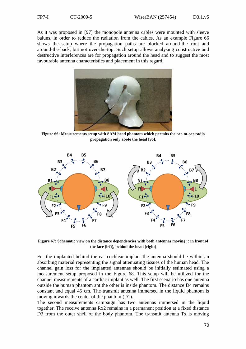
FP7-I CT-2009-5 WiserBAN (257454) D3.1.v5
70
As it was proposed in [97] the monopole antenna cables were mounted with sleeve
baluns, in order to reduce the radiation from the cables. As an example Figure 66
shows the setup where the propagation paths are blocked around-the-front and
around-the-back, but not over-the-top. Such setup allows analysing constructive and
destructive interferences are for propagation around the head and to suggest the most
favourable antenna characteristics and placement in this regard.
Figure 66: Measurements setup with SAM head phantom which permits the ear-to-ear radio
propagation only abote the head [95].
Figure 67: Schematic view on the distance dependencies with both antennas moving: : in front of
the face (left), behind the head (right)
For the implanted behind the ear cochlear implant the antenna should be within an
absorbing material representing the signal attenuating tissues of the human head. The
channel gain loss for the implanted antennas should be initially estimated using a
measurement setup proposed in the Figure 68. This setup will be utilized for the
channel measurements of a cardiac implant as well. The first scenario has one antenna
outside the human phantom ant the other is inside phantom. The distance D4 remains
constant and equal 45 cm. The transmit antenna immersed in the liquid phantom is
moving inwards the center of the phantom (D1).
The second measurements campaign has two antennas immersed in the liquid
together. The receive antenna Rx2 remains in a permanent position at a fixed distance
D3 from the outer shell of the body phantom. The transmit antenna Tx is moving

FP7-I CT-2009-5 WiserBAN (257454) D3.1.v5
71
away from the Rx2 antenna towards the symmetry axis of the cylindrical body
phantom. In other words while distance to the outer shell D3 remains constant the
distance D2 changes.
Figure 68: Measurements scenarios using liquid body phantom

FP7-I CT-2009-5 WiserBAN (257454) D3.1.v5
72
6 On-body Channel modelling for BANs
A common assumption is to define the radio channel as a composite of the linear
wave interactions, which occur between a transmitting and a receiving antenna, and
can be represented by means of a time-varying linear filter characterized by its
impulse response );( th , also known as input-delay spread function according to the
classical Bello’s definition A snapshot of );( th at observation time nt can be
expressed as:
)()();()(
1
nk
tjtK
k
nkn tetath nk
n
(17)
where )( nk ta , nk t and nk t represent respectively the amplitude, phase and delay
of the k-th path, while ntK is the total number of multi path components.
Imposing a limited rectangular bandwidth B, the discrete delays are combined into L
delays bins.
When the delay separation between of a number of paths ( )()( njni tt for
)(,...,2,1, ntNji ) is less than the bin separation BT /1 , they cannot be resolved as
distinct. As a consequence the resolved path is:
nk
n
tjtN
k
nknl etatA
)(
1
)()( (18)
The channel impulse response can be written as:
)(sin)();()(
1
nl
tL
l
nln tBctAthn
(19)
where )( nl t are the discrete time bin.
The time variant transfer function can be expressed as:
dethftH fj2);();(
(20)
By integrating over the frequency we obtain the time dependent power transfer
function averaged over the band of interest:
dfftHB
tPB
2
);(1
)( (21)
where B is the bandwidth of interest. This quantity is often approximated by the RSSI
signal at the receiver.
6.1 Results from the preliminary campaign
6.1.1 Channel gain model
For a given channel transfer function the total power, or channel gain, is given by:
obsT B
obs
dtdfftHBT
G2
0 );(1
(22)
where is the averaging observation period. The channel gain is a key parameter,
which determines the signal-to-noise ratio, averaged over small-scale and large-scale

FP7-I CT-2009-5 WiserBAN (257454) D3.1.v5
73
fading, which can be achieved by the wireless system. The averaging operation over
the bandwidth supposes that all the dielectric constant of materials and all propagation
phenomena related with, do not depend on the frequency. This assumption
corresponds in a certain way to a WSS assumption in Bello’s definitions. In classical
indoor and outdoor channels the is often expressed as a function of antenna
separation. A number of studies in the literature investigated the channel gain, or
equivalently the mean path loss, as a function of the antenna separation, by defining a
path loss coefficient.
Here we use a “scenario-based” approach as explained above. We computed the
channel gain by means of (22) for each scenario and we found a significant variation
between different human subjects. These results can be easily explained by the fact
that even if the antenna position is carefully reproduced on each human subject, the
differences on body shape and dielectric proprieties yield to different path losses.
From measurement results we found that the most appropriate way to describe is a
log-normal distribution. As a consequence the channel gain in dB can be represented
by a Gaussian random variable (r.v.):
SS 000 ,~
dBG (23)
where the mean value and standard deviation depend on the scenario S, as described
above. The statistical analysis is here performed on the mean channel gain of different
subjects, so that normal distribution accounts for the dissimilarities between human
bodies. Some local micro-variations of the antenna emplacement due to dissimilar
body shapes, produce also differences in mean channel gain, and their effect is taken
into account by (23). In Table 19 and Table 20 we list the results for the investigated
scenarios.
TX on Hip
Anechoic chamber Indoor
RX µ0S [dB] σ0S [dB] µ0S [dB] σ0S [dB]
Chest -60.8792 4.15 -54.6518 4.8124
Thigh -64.3146 1.5457 -60.7145 2.6247
Right Wrist -63.2105 2.6178 -57.8699 5.1064
Right Foot -67.1255 5.1838 -60.4444 2.2669
Chest -53.3737 7.8693 -51.7554 7.2704
Thigh -61.9708 6.4907 -59.4894 3.0444
Right Wrist -62.1787 5.9615 -59.592 4.2025
Right Foot -68.6067 7.411 -58.3369 2.5985
Chest -52.7866 3.3482 -47.947 7.5404
Thigh -59.121 4.4368 -57.8446 3.521
Right Wrist -65.8698 4.3149 -61.7829 3.8987
Right Foot -71.2233 8.4303 -60.4773 1.9647
Table 19: Channel gain parameters TX on Hip

FP7-I CT-2009-5 WiserBAN (257454) D3.1.v5
74
TX on Left Ear
Anechoic chamber Indoor
RX µ0S [dB] σ0S [dB] µ0S [dB] σ0S [dB]
Right Ear -63.2533 6.3566 -60.222 3.1504
Hip -60.1378 8.941 -60.2879 6.0754
Right Wrist -72.9014 2.6375 -64.4708 3.2828
Right Foot -75.3591 4.5385 -62.7263 2.191
Right Ear -61.0003 2.7018 -60.0321 3.0879
Hip -57.9352 7.1715 -58.777 4.9483
Right Wrist -71.855 2.9189 -63.0413 1.9839
Right Foot -72.9939 4.6507 -61.0049 1.31
Right Ear -61.3644 3.649 -60.7473 5.3087
Hip -63.8337 7.545 -60.7622 5.706
Right Wrist -71.9968 2.2282 -63.5684 2.2375
Right Foot -77.7146 3.4217 -62.7026 1.1543
Table 20: Channel gain parameters TX on Ear
As shown in Table 19 and Table 20 the dispersion on channel gain can be
considerable especially in anechoic chamber (large ζ0S ), where the propagation
occurs mainly by creeping waves on-body, line-of-sight and by a small reflection on
the ground.
Moreover the path loss is stronger in the anechoic chamber, while in indoor the
propagation occurs by multiple bounces (e.g; reflections, diffractions...) in the
environment, which results into an additional energy contribution. This phenomenon
is particularly clear when the receiving antenna is significantly masked by the human
body. For instance in the Hip-Foot and Ear-Foot links we measured a channel gain up
to 10 dB and 15 dB stronger in the indoor environment. We can remark a more
important dispersion in the Hip-Chest and Ear-Hip links, showing a significant
variability of the human body. When the antennas are placed on torso the propagation
is mainly due to creeping waves and no “on-air” propagation occurs. Thus in these
kinds of scenarios the body shape and composition plays a more important role, which
yields to a large ζ0S .
6.1.2 Shadowing and fading model
It is well-known that one can distinguish a slow fading component ntS and a fast
one ntF in the time-dependent power transfer function:
nnn tFtSGtP 0 (24)
We extracted from our measurements the slow fading component by applying a low
pass filter, practically realized by averaging the time-dependent power transfer
function on a sliding temporal window.
The slow component is basically due to the shadowing by human body. As shown in
Figure 69, the shadowing strictly depends on the movement condition. When the
human subject does not move the slow component is quite moderated, since the
shadowing condition basically remains identical. The shadowing also depends on the

FP7-I CT-2009-5 WiserBAN (257454) D3.1.v5
75
way of moving of each human subject. Figure 70 shows for instance that the
amplitude of the slow component is larger in subject B than D, since one oscillates his
arms more the other one, when walking.
The statistical analysis on the slow component has been carried out on the time
dependent samples dBntS )( of the whole population of the human subjects. It has been
found that the shadowing in dB follows a normal distribution:
SsdBntS ,0~)( (25)
where the standard deviation Ss accounts for the slow variations of the power transfer
function given by shadowing from human body, in a specific scenario.
Figure 69: Time-variant power transfer function and slow fading in indoor: TX on Hip, 2.45 GHz
band, still (left) and walking subject (right)
Figure 70: Shadowing for human subject B and D: Walking Hip-to-Wrist link
In Table 21 and Table 22 we list the values of Ss when TX is on Hip. As expected
we have a larger standard deviation in moving scenario. It is interesting to notice that
the larger variations around the mean value have been found in the walking case. The
standard deviation of the running subject is smaller than the walking one, since people
tend to keep arms close to the body, limiting their oscillating movement. Similarly,
the legs’ movement is faster than in the walking scenario but, since the subject keeps
standing on the same spot, the feet do not move backwards and forwards in a circular

FP7-I CT-2009-5 WiserBAN (257454) D3.1.v5
76
arc with respect to the body axis. As a consequence the shadowing condition is less
time-varying than in the walking scenario, which results into a smallerSs . Moreover
the slow fading effect is smaller in indoor since the propagation occurs also by
reflection on the surrounding environment, which somewhat mitigate the shadowing
by human body. The two random variables describing the channel gain and
shadowing are obtained by statistical analysis on human body variability and human
body movement, so that it is reasonable to consider that they are uncorrelated. As a
consequence the channel gain (in dB) presents a slow variation around the mean
valueS0 , which is described by a total variance
22
0 SS s .
TX on Hip
Chest Thigh R Wrist R Foot
Anech
oi
c
Still 0.6329 0.4269 1.0185 0.4564
Walking 2.2892 5.4279 4.4565 5.2028
Running 2.3997 2.5117 3.6504 2.8322
Indo
or Still 0.638 0.2578 0.2706 0.2593
Walking 1.6049 3.486 2.7915 2.734
Running 2.0977 2.0965 2.5062 1.8854
Table 21: Shadowing parameters TX on Hip
TX on Left Ear
R ear Hip R Wrist R Foot
Anech
oi
c
Still 0.7205 1.1237 1.781 0.8133
Walking 0.7293 2.1193 3.5141 4.4149
Running 0.5409 2.9261 3.1742 1.7009
Indo
or Still 0.5768 1.5246 0.8373 0.7621
Walking 0.9393 2.2444 1.8723 2.1241
Running 0.7259 2.282 1.9811 1.3007
Table 22: Shadowing parameters TX on Ear
The shadowing effect discussed above, represents a large scale variation of the power
transfer function which is mainly due to the masking effect by human body.
Nevertheless a fast fading component is also present, as depicted in Figure 69.
Obviously by integrating over a large bandwidth in (22) the fast fading is sensibly
reduced. As a consequence here we focus on the power transfer function at single
frequency at 2.45 GHz. The bandwidth is implicitly the one employed in
measurements, i.e. 10 MHz. The slow fading is extracted by applying a sliding
temporal window.
Table 23: Fading characteristics at 2.45 GHz (B =10 MHz): TX on Hip, Indoor, walking
scenarios.

FP7-I CT-2009-5 WiserBAN (257454) D3.1.v5
77
In Table 23 we report the slow and fast fading characteristics when the human subject
walks in an indoor environment. The fading duration is computed as the average time
below the mean value. Measurement results show that the fade duration can affect
directly the single symbol transmission, while the shadowing can affect the packet
one (Table 24).
Measurement results show that fast fading follows a Rice distribution:
202
22
2 2exp
Ipdf (26)
Where 0I
represents the modified Bessel function of the first kind with order zero,
and and are the parameters of the distribution. Figure 71 shows the good
agreement of data and the Rice model, in the walking and running scenarios.
Figure 71: Fast fading distribution in indoor: TX on Hip, walking (left) and running (right).
In Table 24 we list the parameters of the Rice distribution of nt obtained by
Akaike method from measurement results. Results show a high k-factor
( é
xK 2/2 ) when the human subject does not move, which means that there is a
main path with a strong energy contribution. As a consequence the channel
experiment a little fast fading, which is mainly due to involuntary breathing
movements. In walking scenarios, the K-factor is low, which results in a more
important fast fading. For instance in the Hip-Foot link the nodes are often masked by
the body and propagation occurs by reflection on surrounding environments. As a
consequence K-factor is close to 0 and we can approximate the fading statistic with a
Rayleigh distribution.
Table 24: Fading statistics at 2.45 GHz (B =10 MHz): TX on Hip, Indoor.
When moving from anechoic chamber to indoor scenario the multi-paths coming from
surrounding scatterers superpose to the purely on-body propagation (i.e. diffraction on
the body and transmission in line of sight). Since each multi-path component yields an
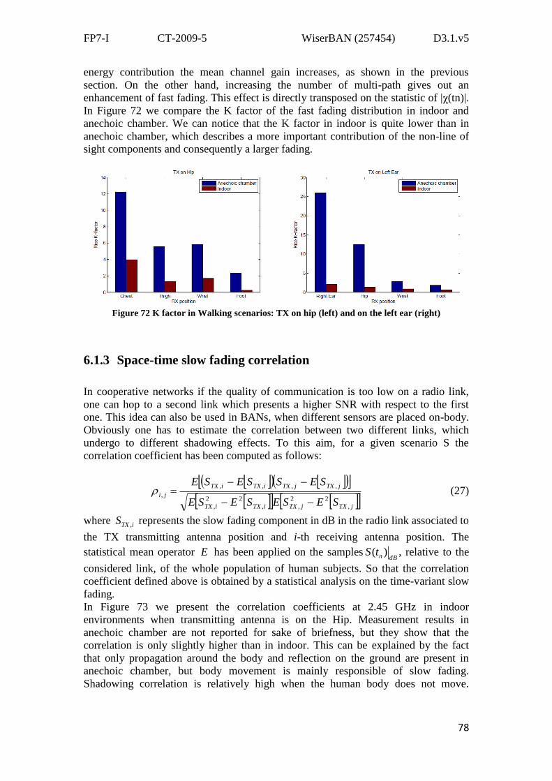
FP7-I CT-2009-5 WiserBAN (257454) D3.1.v5
78
energy contribution the mean channel gain increases, as shown in the previous
section. On the other hand, increasing the number of multi-path gives out an
enhancement of fast fading. This effect is directly transposed on the statistic of |χ(tn)|.
In Figure 72 we compare the K factor of the fast fading distribution in indoor and
anechoic chamber. We can notice that the K factor in indoor is quite lower than in
anechoic chamber, which describes a more important contribution of the non-line of
sight components and consequently a larger fading.
Figure 72 K factor in Walking scenarios: TX on hip (left) and on the left ear (right)
6.1.3 Space-time slow fading correlation
In cooperative networks if the quality of communication is too low on a radio link,
one can hop to a second link which presents a higher SNR with respect to the first
one. This idea can also be used in BANs, when different sensors are placed on-body.
Obviously one has to estimate the correlation between two different links, which
undergo to different shadowing effects. To this aim, for a given scenario S the
correlation coefficient has been computed as follows:
jTXjTXiTXiTX
jTXjTXiTXiTX
ji
SESESESE
SESSESE
,
22
,,
22
,
,,,,
,
(27)
where iTXS , represents the slow fading component in dB in the radio link associated to
the TX transmitting antenna position and i-th receiving antenna position. The
statistical mean operator E has been applied on the samplesdBntS )( , relative to the
considered link, of the whole population of human subjects. So that the correlation
coefficient defined above is obtained by a statistical analysis on the time-variant slow
fading.
In Figure 73 we present the correlation coefficients at 2.45 GHz in indoor
environments when transmitting antenna is on the Hip. Measurement results in
anechoic chamber are not reported for sake of briefness, but they show that the
correlation is only slightly higher than in indoor. This can be explained by the fact
that only propagation around the body and reflection on the ground are present in
anechoic chamber, but body movement is mainly responsible of slow fading.
Shadowing correlation is relatively high when the human body does not move.

FP7-I CT-2009-5 WiserBAN (257454) D3.1.v5
79
Nevertheless the small value of Ss reduces the correlation significance in Still
scenarios.
The scenarios which present high shadowing (generally when one antenna is on a
limb) present the highest correlation. For instance in walking scenarios the Hip-Wrist,
Hip-high and Hip-Foot are strongly correlated. It is very interesting to see that
correlation is inverted for Wrist/Thigh and Wrist/Foot. This is due to the fact that the
receiving antennas are all on right limbs while the transmitting antenna is on the left
side. During a walk, humans tend to alternate the movement of legs and arms. As a
consequence shadowing on right wrist is the opposite of shadowing on right thigh and
right foot, while shadowing on foot and thigh follow the same temporal behaviour (as
depicted in Figure 73. This macro effect is verified in both anechoic and indoor
environments. Finally in running scenarios the shadowing on limbs are more
correlated than shadowing on chest, but generally less correlated than in walking
scenarios. This is due to the fact that the human subjects have less control on the
synchronism of movements, which results into a higher asynchronism of shadowing
thus a lower correlation.
Figure 73: Correlation coefficients: TX on Hip
6.1.4 Doppler spectrum modelling
In classical time-variant channel models, the mobility is often taken into account by a
movement of the receiving antenna at speed v with respect to the transmitting one. By
considering that a small movement, corresponding to a time separation t , the
amplitude and phase of the k-th MPC can be considered constant, while the phase
variation is ktv cos/2
In the case of isotropic scattering, the received
signals come from all directions with equal probabilities. The isotropic scattering
model, also known as the Clarke’s model, corresponds to the uniform distribution for
the angle of arrival [,[ k . This assumption and hypothesis of uncorrelated
scatters (US) yields to the classical Jake’s bath-tube like Doppler spectrum [101] .
Previous works on indoor channel with fixed antennas and moving scenarios have
highlighted Doppler behaviour different from the Jakes/Clarke model [102] ,[103] . In
these scenarios the time variance of the channel is given by the people movement in
the environment where the fixed antennas are placed. The Doppler spectrum in this
case is centred around a mean value at 0 Hz and can be modelled by a Laplacian
distribution [104].
In BANs the antennas are placed on-body, and the human subject is set free to move.
The scatters are given by the surrounding environment and the human body itself. In

FP7-I CT-2009-5 WiserBAN (257454) D3.1.v5
80
practical situations the antennas reciprocal positions do not vary significantly, while
the scatters position, with respect to the TX-RX link, can change with the human
movement. Thus the on-body channel can be assumed, in a first approximation, as a
fixed TX-RX situation with moving scatters, producing the time variance of the
channel. This assumption is quite correct when both transmitting and receiving
antennas are placed on the torso or on the same limb, or, more generally, when there
is a slight movement of the receiver antenna with respect to transmitter (e.g. Hip-Foot
link, and arm swinging). In these cases the Doppler function is centred at = 0 Hz.
In anechoic chamber no scatters are present with except the body itself. In Figure 74
we show the normalized Doppler Spectra at 2.4 GHz, when the human subject walks
in anechoic chamber. When one antenna is on the torso and the other on a moving
limb, the distance between TX and RX can change slightly. However the velocity of
the receiving antenna with respect to the transmitting one is very low, and the time-
variance is mainly given by the varying position of the scatters. As a consequence the
Doppler function is still centred at = 0, but it presents a smoother behaviour, as
shown in Figure 74.
Figure 74: Normalized Doppler Spectra: human walking in anechoic chamber
The difference between the levels of the floor when the receiving node is on the chest,
with respect to the nodes on the limbs, can be explained by the increased degree of
mobility in the latter case. Given this behaviour of the Doppler spectra it is useful to
identify the bandwidths with respect to a threshold, e.g. -20 dB below the peak value
at 0 Hz, instead of the maximum Doppler Shift. In Table 25 we list the results
obtained from our measurements in anechoic chamber.
A rigorous mathematical formulation of Doppler spectrum from moving scatterers
has been recently given in [105]. By assuming uniform scattering pattern and
independence of scatterers, the Doppler spectrum can be decomposed by Bessel and
Legendre functions. Instead of Laplacian distribution a simplified expression of the
normalized Doppler spectrum can be the following:
2
1)(
BODYOND (28)

FP7-I CT-2009-5 WiserBAN (257454) D3.1.v5
81
In Figure 74 we show the good approximation of this model with the measurement
results, by using the values of listed in Table 25. A small value of represents a
modest degree of mobility, as in the Hip-Chest, Ear-Ear and Ear-Hip links.
Table 25: Doppler Bandwidth at -20 dB and model parmeter of on-body Doppler
Some important differences can be noticed when moving from the anechoic scenario
to a realistic one. In Figure 75 we show the normalized average power of effective
scattering distribution, for the Hip to Wrist channel in walking scenarios. When the
human subject is in anechoic chamber, since no off-body scatterers are present, most
of energy is concentrated around 3ns, which is close to time-of-flight between the
node locations. The effective scattering distribution presents a high peak at the
frequency Doppler = 0. When human subjects are in indoor environment we can
clearly identify some off-body scatterers, far away from the on-body ones. It is
interesting to notice that the presence of these scatterers yields to no-symmetric
scattering distribution. This is mainly due to the fact that the antennas are placed on
the front side of the body. As a consequence the scatterers in a half space behind the
body are strongly masked by the shadowing of the body itself.
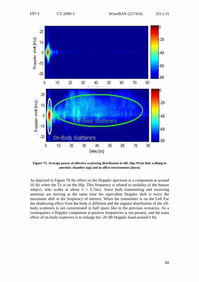
FP7-I CT-2009-5 WiserBAN (257454) D3.1.v5
82
Figure 75: Average power of effective scattering distribution in dB: Hip-Wrist link walking in
anechoic chamber (up) and in office environment (down)
As depicted in Figure 76 the effect on the Doppler spectrum is a component at around
10 Hz when the Tx is on the Hip. This frequency is related to mobility of the human
subject, who walks at about v = 0.7m/s. Since both transmitting and receiving
antennas are moving at the same time the equivalent Doppler shift is twice the
maximum shift at the frequency of interest. When the transmitter is on the Left Ear
the shadowing effect from the body is different and the angular distribution of the off-
body scatterers is not concentrated in half space like in the previous scenarios. As a
consequence a Doppler component at positive frequencies is not present, and the main
effect of on-body scatterers is to enlarge the -20 dB Doppler band around 0 Hz

FP7-I CT-2009-5 WiserBAN (257454) D3.1.v5
83
Figure 76: Normalized Doppler Spectra by human walking in anechoic chamber: TX on Hip
(up), TX on Left Ear (down)
When a well-identified Doppler component is present, like in the on Hip scenario, is it
possible to separate the off-body scatterer Doppler contribution from the purely on-
body one. In these cases one can express the total Doppler Spectrum as the
combination of two independents factors:
)()()( BODYOFFBODYONTOT DDD (29)
where BODYOND is the component related to the on-Body scatterers, as in (28), and
)(BODYOFFD to the off-body ones. Obviously the factorization of these two
components is a strong approximation, but it yields to a simple model. In the
scenarios with TX on the Hip, it was found that the off-boy presents a Gaussian shape
in dB:
2
2
02
exp)(
m
dBBODYOFF DD
(30)
-20 -10 0 10 20-40
-35
-30
-25
-20
-15
-10
-5
0
Nor
m.
Dop
pler
Spe
ctru
m [
dB]
Doppler Shift [Hz]
L Ear-R Ear
L Ear-Hip
L Ear-Wrist
L Ear-Foot
-25 -20 -15 -10 -5 0 5 10 15 20 25-45
-40
-35
-30
-25
-20
-15
-10
-5
0
Norm
aliz
ed D
opple
r S
pectr
um
Doppler shift [Hz]
Hip-Chest
Hip-Thigh
Hip-Wrist
Hip-Foot

FP7-I CT-2009-5 WiserBAN (257454) D3.1.v5
84
In Figure 77 we show the good agreement between measurements and the model
expressed in (29). Table 26 lists the parameters of Doppler Spectrum for some
scenarios in indoor on-body channels. It is interesting to notice that the off-body
component presents in all scenarios a mean value around 10 Hz, showing some
reproducibility of the effect of the off-body scatterers.
Figure 77: Normalized Doppler Spectra: human walking in Indoor, Hip- Wrist Channel
Table 26: Doppler parameters in indoor
The knowledge of Doppler Spectrum allows the quantification of how much
broadening is imposed on the spectrum of signal, according to the rate of change in
the channel state. In multi-path scenarios the Doppler shift of each path can be
different from that of another path, which results into a Doppler spreading. The
Doppler spread can be used to evaluate the time-variance of the channel and estimate
the coherence time at 0.5 correlation threshold and shown in Figure 78, [106] .
Figure 78: Choerence time: TX on Hip (left), on Ear (right)
-20 -10 0 10 20-30
-25
-20
-15
-10
-5
0
Doppler Frequency Shift [Hz]
Norm
. D
opple
r S
pectr
um
Measurement
Model

FP7-I CT-2009-5 WiserBAN (257454) D3.1.v5
85
6.2 Full measurement campaign results
Starting from the same assumptions presented in the previous section, the studies
performed on the acquired data aim at extracting a complete on-body channel model
through the description of the three different components constituting the time-
dependent channel power transfer function P(t). Considering the “scenario-based”
approach, all the results presented will refer to a specific scenario Body-OnS that will be
clarified every time when needed.
6.2.1 Channel gain model
The mean channel gain G0 is here computed by means of (22), by considering Tobs is
the duration of the acquisition set to 3 seconds, and B is the bandwidth considered
equal to 10 MHz and centred on the carrier frequency 2.45 GHz.
In order to consider the variation on channel gain related to the characteristics of the
body, it is more appropriate to describe the channel gain in dB giving its mean value
(μ0S) and standard deviation (σ0S) for every investigated scenario Body-OnS .
Table 27, Table 28 and Table 29 list the values obtained, sorted by scenario. It’s
worth to remember that channel model for the sitting/standing scenario and Tx on hip
is not available, since measurements were not performed.
Tx Heart - Top Loaded Monopole Tx Heart - Planar Monopole
Quasi-anechoic chamber
Indoor Office Quasi-anechoic
chamber Indoor Office
Rxs μ0S [dB] σ0S [dB] μ0S [dB] σ0S [dB] μ0S [dB] σ0S [dB] μ0S [dB] σ0S [dB]
Walking Right Thigh -38,45 1,06 -38,65 1,15 -66,77 3,35 -62,72 2,41
Rigth Hand -47,07 2,16 -49,47 1,2 -63,87 6 -60,15 5,79
Left Hand -43,86 2,46 -42,97 3,19 -60,42 4,35 -58,35 1,5
Left Ear -48,62 3,62 -46,82 4,57 -61,06 5,18 -60,48 3,5
Sitting/ Standing
Right Thigh -39,45 1,59 -41,04 1,44 -63,96 5,36 -58,02 3,61
Rigth Hand -46,54 2,46 -47,73 4,6 -58,41 2 -56,06 4,89
Left Hand -43,52 2,35 -43,02 2,76 -54,62 3,07 -56,21 3,53
Left ear -48,34 2,43 -43,47 1,98 -63,07 2,72 -59,13 4,47
Standing Still
Right Thigh -38,75 0,92 / / -68,34 4,92 / /
Rigth Hand -46,58 1,69 / / -66,25 6,17 / /
Left Hand -42,12 1,87 / / -62,43 2,36 / /
Left Ear -45,01 1,36 / / -60,96 2,27 / /
Table 27: Channel Gain values for scenarios where Tx is placed on Heart

FP7-I CT-2009-5 WiserBAN (257454) D3.1.v5
86
Tx Left Hip - Top Loaded Monopole Tx Left Hip - Planar Monopole
Quasi-anechoic chamber
Indoor Office Quasi-anechoic
chamber Indoor Office
Rxs μ0S [dB] σ0S [dB] μ0S [dB] σ0S [dB] μ0S [dB] σ0S [dB] μ0S [dB] σ0S [dB]
Walking Right Thigh -38,78 2,06 -38,4 1,17 -63,85 2,4 -60,77 4,89
Rigth Hand -52,09 4,58 -53,09 2,89 -67,54 7,5 -61,69 6,9
Left Hand -40,32 3,17 -40,74 4,32 -50,38 1,08 -49,62 2,95
Left Ear -47,24 2,02 -48,3 2,69 -68,45 5,4 -64,26 3,3
Standing Still
Right Thigh -42,78 2,26 / / -61,17 1,06 / /
Rigth Hand -48,35 4,8 / / -68,97 1,29 / /
Left Hand -34,52 1,37 / / -47,59 2,4 / /
Left Ear -46,77 1,46 / / -69,77 3,63 / /
Table 28: Channel Gain values for scenarios where Tx is placed on Left Hip
Tx Right Ear - Top Loaded Monopole Tx Right Ear - Planar Monopole
Quasi-anechoic chamber
Indoor Office Quasi-anechoic
chamber Indoor Office
Rxs μ0S [dB] σ0S [dB] μ0S [dB] σ0S [dB] μ0S [dB] σ0S [dB] μ0S [dB] σ0S [dB]
Walking Right Thigh -55,13 3,29 -57,57 1,84 -72,53 5,96 -67,01 2,77
Rigth Hand -53,82 3,92 -53,31 3,19 -64,61 4,49 -59,18 2,27
Left Hand -66,59 4,98 -57,57 0,91 -74,89 2,63 -65,67 4,63
Left Ear -35,81 0,82 -37,01 2 -58,54 6,05 -54,67 4,73
Sitting/ Standing
Right Thigh -56,77 2,99 -57,78 2,56 -72,27 3,58 -65,93 4,41
Rigth Hand -54,2 2,97 -55,18 1,95 -61,83 5,41 -61,22 2,5
Left Hand -61,52 3,62 -58 1,52 -73,82 3,26 -64,79 3,63
Left ear -36,33 1,56 -36,43 2,08 -57,41 8,28 -55,44 6,33
Standing Still
Right Thigh -53,82 1,99 / / -76,22 3,05 / /
Rigth Hand -49,92 2,47 / / -67,77 2,47 / /
Left Hand -66,87 3,43 / / -78,83 2,05 / /
Left Ear -33,69 0,81 / / -68,02 4,12 / /
Table 29: Channel Gain values for scenarios where Tx is placed on Right Ear
The analysis has been performed gathering the mean channel gain of the four different
subjects, so that the standard deviation ζ0S accounts for the heterogeneity brought by
the human bodies in terms of body shape and dielectric properties. Moreover, even if
the nodes emplacement is carefully reproduced, some local micro-variations of their

FP7-I CT-2009-5 WiserBAN (257454) D3.1.v5
87
position could produce differences in the mean channel gain values, which are also
considered in ζ0S.
The numerical results presented in Table 27, Table 28 and Table 29 are useful in order
to make some comparative considerations between the two different sets of antennas
(for more details see Paragraph 4.1.2 and Paragraph 4.1.3) and the influence of the
environments where the measurements have taken place.
First of all, it is possible to remark how the path loss is generally stronger when
Planar Monopole antennas (PL Monopole) have been used, comparing to the case
with Top Loaded Monopole (TL Monopole), as shown in Figure 79. As expected, the
antenna with normal polarisation with respect to the body surface (TL Monopole) is
more suited for On-Body applications, supporting the creeping-waves propagation
over the body. This leads to higher values in terms of channel gain up to 22-25dB
with respect to the ones found for tangentially polarised antennas (PL Monopole).
This effect is particularly evident for those channels with a strong on-body
propagation component and where no “on-air” propagation occurs, such as Heart-
Thigh, Hip-Thigh and Ear-Ear links.
0 0.5 1 1.5 2 2.5-80
-75
-70
-65
-60
-55
-50
-45
-40
-35
-30G0 vs. Anetnna Type - Anechoic Chamber - Tx Hip - Standing Still
Time [s]
Channel G
ain
[dB
]
Rx Left Ear, P(t)
Rx Left Ear, G0
Rx Left Hand, P(t)
Rx Left Hand, G0
Rx Right Hand, P(t)
Rx Right Hand, G0
Rx Right Thigh, P(t)
Rx Right Thigh, G0
PLMonopole
TLMonopole
Figure 79: G0 comparison for different antenna sets
For PL Monopoles it could also be pointed out that the dispersion on the channel gain
is relevant especially in quasi-anechoic environment, where the ζ0S values are larger
than those found for the indoor scenario. Same considerations could not be drawn for
the TL Monopole case, where the standard deviations are generally smaller than in the
former case and the difference between indoor and anechoic environment is not so
stressed. This is due to the fact that the presence of a ground plane makes the antenna
less influenced but the human body.
The different behavior of the two sets of antennas in respect with the environment
considered could be explained assuming that in anechoic chamber the propagation
occurs mainly by creeping waves on-body and small reflection on the ground, and

FP7-I CT-2009-5 WiserBAN (257454) D3.1.v5
88
these phenomena affects more the performances of tangentially polarized antennas,
like the PL Monopole, than those of antennas with normal polarization.
It could also be noticed that, for the PL antenna, the mean path loss is stronger in the
anechoic chamber than in indoor, because in the latter environment the multi-paths
contribution due to reflections and diffractions from the environment is very
significant, leading to an additional energy contribution. This trend is more evident
when one of the nodes composing the link is considerably masked by the human
body. For instance, channel gain stronger up to 10 dB in indoor than anechoic
chamber have been measured for the Right Ear-Left Hand channel, where the whole
body shadows the communication.
For the same reasons explained above, this is not at all valid for the TL Monopoles,
where all the scenarios present almost the same values for the channel gain.
A graphical example is given in Figure 80:
0 0.5 1 1.5 2 2.5-85
-80
-75
-70
-65
-60
-55
-50G0 for TL Monopole vs. Environment - Tx Ear - Rx Thigh - Sitting
Time [s]
Channel G
ain
[dB
]
Rx Right Thigh, P(t), Indoor
Rx Right Thigh, G0, Indoor
Rx Right Thigh, P(t), Anechoic
Rx Right Thigh, G0, Anechoic
0 0.5 1 1.5 2 2.5-85
-80
-75
-70
-65
-60
-55
-50G0 for PL Monopole vs. Environment - Tx Ear - Rx Thigh - Sitting
Time [s]
Channel G
ain
[dB
]
Rx Right Thigh, P(t), Indoor
Rx Right Thigh, G0, Indoor
Rx Right Thigh, P(t), Anechoic
Rx Right Thigh, G0, Anechoic
Figure 80: G0 values in different environment for PL Monopole (up) and TL Monopole (down)

FP7-I CT-2009-5 WiserBAN (257454) D3.1.v5
89
6.2.2 Shadowing and fast fading model
As pointed out in (24) the time-dependent power transfer function is also defined by a
slow fading or shadowing S(t) and a fast fading F(t) components. In order to extract
S(t) from the data acquired, a low pass filter has been applied to P(t), practically
realised by averaging it on a sliding temporal window, letting the slow variations of
this function to be followed.
0 0.5 1 1.5 2 2.5-60
-55
-50
-45
-40
-35
-30Anechoic Chamber - Tx Heart - Top Loded Monopole - Still
Time [s]
Channel G
ain
[dB
]
Rx Thigh, P(t)
Rx Thigh, G0*S(t)
Rx Right Hand, P(t)
Rx Right hand, G0*S(t)
Rx Left Hand, P(t)
Rx Left Hand, G0*S(t)
Rx Left Ear, P(t)
Rx Left Ear, G0*S(t)
0 0.5 1 1.5 2 2.5 3-70
-65
-60
-55
-50
-45
-40
-35
-30Indoor - Tx Hip - Top Loaded Monopole - Walking
Time [s]
Channel G
ain
[dB
]
Rx Thigh, P(t)
Rx Thigh, G0*S(t)
Rx Right Hand, P(t)
Rx Right Hand, G0*S(t)
Rx Left Hand, P(t)
Rx Left hand, G0*S(t)
Rx Left Ear, P(t)
Rx Left Ear, G0*S(t)
Figure 81: Time-variant power transfer function and slow fading component: standing still (up)
and walking (down) conditions
In wireless communications, the slow fading component accounts for the shadowing
effect of some obstacles that obstruct the direct link between nodes. For the specific
case of BANs this term is strictly connected to the shadowing produced by the human
body itself, and heavily depends on the movement conditions. This effect is
graphically represented in Figure 81 where it is possible to notice that when the
subject stands still (up) in the same position, the shadowing component is almost

FP7-I CT-2009-5 WiserBAN (257454) D3.1.v5
90
constant, and the only slight variations of P(t) are due the involuntary breathing
movements. On the other side, the shadowing effect of the human body is stronger
when the subject walks (down), in particular for those links where one node is placed
on a limb. For example, focusing on the Hip-Right Hand link, it is possible to
reconstruct the walking movement following the shadowing trend and considering
that the subject swings his arms cyclically.
It is interesting to notice how Thigh and Hand links show negative correlation, as
shown by red (Right Tight) and blue (Right Hand) lines in Figure 81. Their trends
follow opposite pattern since, during a normal walk, hands swing opposite to the legs
movements.
It is also worth noticing that every subject walks or, in general, moves in a different
way, and this obviously affects the shadowing trend. This dispersion is more evident
for those links where at least one of the nodes is placed on a limb (i.e. hand or thigh)
and Figure 82 gives an example of how differently two subjects could move in
walking (up) and sitting down/standing up (down) conditions.
0 0.5 1 1.5 2 2.5-10
-8
-6
-4
-2
0
2
4
6
8
10
Time [s]
Shadow
ing [
dB
]
Tx Heart - Rx Left Hand - TL Monopole - Walking
Subject C
SubjectD
0 0.5 1 1.5 2 2.5-10
-8
-6
-4
-2
0
2
4
6
8
10Tx Heart - Rx Left Hand - PL Monopole - Sitting
Time [s]
Shadow
ing [
dB
]
Subeject C
Subject D
Figure 82: Different subjects’ movement in walking (up) and sitting down/standing up (down)
conditions. Heart-Hand link.
In order to completely describe the slow fading component S(t), a statistical analysis
has been performed gathering the acquired data of all the subject sorted by scenario

FP7-I CT-2009-5 WiserBAN (257454) D3.1.v5
91
Body-OnS . As in the previous section, it has been found that the shadowing in dB
follows a normal distribution SsdBntS ,0~)( , where the standard deviation ζSS
accounts for the slow variations of the power transfer function given by the
shadowing from human body, in a specific scenario. As an example of the statistic
given, Figure 83 presents the normal fitting obtained for the shadowing values in dB
for the scenario with PL Monopole in anechoic chamber when the Tx is placed on the
Hip.
-15 -10 -5 0 5 10 150
0.02
0.04
0.06
0.08
0.1
0.12
0.14
0.16
0.18
0.2
S(tn)
Anchoic Chamber - Planar Monopole - Tx Hip - Walking
PD
F
Rx Thigh, S(tn)
Fit Rx Thigh, S(tn)
Rx Right Hand, S(tn)
Fit Rx Right hand, S(tn)
Rx Left Hand, S(tn)
Fit Rx Left Hand, S(tn)
Rx Left Ear, S(tn)
Fit Rx Left Ear, S(tn)
Figure 83: Probability Density Function of shadowing in anechoic environment for PL Monopole
in walking conditions
The statistical description of the shadowing has been given through its standard
deviation ζSS , as well as other characteristic parameters like the mean duration of the
fade in ms, its mean depth in dB and the rate of appearance in s-1
.
The characterisation has been performed for every combination of antenna,
environment and moving condition, as reported in Table 30, Table 31, Table 32,
Table 33, Table 34 and Table 35.

FP7-I CT-2009-5 WiserBAN (257454) D3.1.v5
92
Shadowing statistics - Top Loaded Monopole - Tx Heart
Walking Sitting Down / Standing Up
Rxs σS
Duration [ms]
Depth [dB]
Rate [s
-1]
σS Duration
[ms] Depth [dB]
Rate [s
-1]
Anechoic Chamber
Right Thigh 1,07 554 -1,12 0,88 2,01 535 -2,76 0,71
Rigth Hand 3,46 664 -5,53 0,58 2,15 713 -2,67 0,57
Left Hand 3,67 540 -4,93 0,72 2,57 588 -4,27 0,72
Left Ear 1,06 616 -0,97 0,72 1,12 706 -1,52 0,62
Indoor Right Thigh 1,4 488 -2,31 0,79 3,22 764 -4,91 0,54
Rigth Hand 2,57 517 -3,39 0,79 3,85 880 -7,8 0,38
Left Hand 1,97 546 -3,28 0,75 2,83 590 -3,92 0,63
Left ear 1,5 404 -1,87 1 0,9 507 -1,09 0,86
Table 30: Shadowing statistics for TL antenna Tx on Heart
Shadowing statistics - Planar Monopole - Tx Heart
Walking Sitting Down / Standing Up
Rxs σS
Duration [ms]
Depth [dB]
Rate [s
-1]
σS Duration
[ms] Depth [dB]
Rate [s
-1]
Anechoic Chamber
Right Thigh 3,2 536 -4,1 0,81 4,09 631 -5,58 0,67
Rigth Hand 4,34 556 -6,1 0,75 3,13 698 -3,87 0,57
Left Hand 4,33 660 -4,89 0,71 5,25 871 -8,26 0,43
Left Ear 0,97 663 -0,93 0,67 1,15 702 -1,3 0,63
Indoor Right Thigh 1,82 322 -1,57 1,38 3,14 678 -4,27 0,58
Rigth Hand 2,99 338 -1,98 1,42 4,42 688 -5,66 0,58
Left Hand 4,21 612 -5,55 0,75 4,93 681 -6,26 0,63
Left ear 1,96 321 -1,88 1,25 2,39 542 -3,01 0,75
Table 31: Shadowing statistics for PL antenna Tx on Heart
Shadowing statistics - Top Loaded Monopole - Tx Left Hip
Walking Sitting Down / Standing Up
Rxs σS
Duration [ms]
Depth [dB]
Rate [s
-1]
σS Duration
[ms] Depth [dB]
Rate [s
-1]
Anechoic Chamber
Right Thigh 1,43 551 -1,77 0,75 / / / /
Rigth Hand 4,05 380 -4,58 1 / / / /
Left Hand 3,73 564 -5,27 0,67 / / / /
Left Ear 1,35 478 -1,87 0,84 / / / /
Indoor Right Thigh 1,01 345 -1,2 1,13 / / / /
Rigth Hand 3,98 484 -5,04 0,84 / / / /
Left Hand 3,45 514 -4,33 0,84 / / / /
Left ear 2,79 397 -2,75 1 / / / /
Table 32: Shadowing statistics for TL antenna Tx on Left Hip

FP7-I CT-2009-5 WiserBAN (257454) D3.1.v5
93
Shadowing statistics - Planar Monopole - Tx Left Hip
Walking Sitting Down / Standing Up
Rxs σS
Duration [ms]
Depth [dB]
Rate [s
-1]
σS Duration
[ms] Depth [dB]
Rate [s
-1]
Anechoic Chamber
Right Thigh 3,49 360 -4,39 1,21 / / / /
Rigth Hand 6,07 529 -9,5 0,67 / / / /
Left Hand 7,17 520 -10,45 0,76 / / / /
Left Ear 3,4 600 -3,61 0,72 / / / /
Indoor Right Thigh 3,05 560 -3,42 0,84 / / / /
Rigth Hand 3,76 730 -5,88 0,58 / / / /
Left Hand 7,22 506 -11,43 0,72 / / / /
Left ear 2,38 328 -1,98 1,3 / / / /
Table 33: Shadowing statistics for PL antenna Tx on Left Hip
Shadowing statistics - Top Loaded Monopole - Tx Right Ear
Walking Sitting Down / Standing Up
Rxs σS
Duration [ms]
Depth [dB]
Rate [s
-1]
σS Duration
[ms] Depth [dB]
Rate [s
-1]
Anechoic Chamber
Right Thigh 4,06 570 -5,88 0,71 2,89 605 -3,42 0,62
Rigth Hand 2,25 588 -2,34 0,79 3,82 1000 -4,95 0,5
Left Hand 2,53 383 -2,77 1,23 6,73 803 -8,49 0,53
Left Ear 0,12 634 -0,15 0,71 0,2 780 -0,14 0,58
Indoor Right Thigh 3,17 379 -2,81 1,34 2,08 415 -2,16 1,29
Rigth Hand 2,89 363 -2,65 1,05 2,08 407 -1,85 1,09
Left Hand 1,72 306 -1,38 1,09 2,19 302 -1,85 1
Left ear 0,67 388 -0,83 0,89 0,59 423 -0,48 1,13
Table 34: Shadowing statistics for TL antenna Tx on Right Ear
Shadowing statistics - Planar Monopole - Tx Right Ear
Walking Sitting Down / Standing Up
Rxs σS
Duration [ms]
Depth [dB]
Rate [s
-1]
σS Duration
[ms] Depth [dB]
Rate [s
-1]
Anechoic Chamber
Right Thigh 2,91 345 -3,95 1 3,94 720 -5,19 3,94
Rigth Hand 2,42 545 -2,53 0,84 3,11 577 -3,35 3,11
Left Hand 6,4 613 -4,19 0,81 3,82 649 -4,77 3,82
Left Ear 0,67 855 -1,26 0,47 0,71 737 -0,67 0,71
Indoor Right Thigh 2,23 336 -2,13 2,23 2,21 377 -1,91 2,21
Rigth Hand 2,58 428 -2,89 2,58 2,71 397 -2,41 2,71
Left Hand 2,37 411 -2,55 2,37 2,43 445 -2,68 2,43
Left ear 2,15 501 -2,87 2,15 1,75 355 -1,71 1,75
Table 35: Shadowing statistics for PL antenna Tx on Right Ear

FP7-I CT-2009-5 WiserBAN (257454) D3.1.v5
94
The data presented could draw to some interesting conclusions: in general the
shadowing effect results smaller in indoor premises than in anechoic chamber, leading
to smaller values of ζS. This is reasonable considering that in indoor the propagation
occurs also by reflections on the environment, which somehow mitigate the
shadowing due to human body movement. This is true for all the links except for
those where the receiver is placed on the left ear, probably due to the particular
position of the node.
Figure 84 helps in better understanding the effect explained above. The particular
examples refer to the PL Monopole used in walking scenario for the Tx placed on the
Heart, it is possible to notice that the indoor shadowing, i.e. continuous lines, (Figure
84 up) is in general less varying) than in anechoic (down). This yields to (smaller
value of the shadowing standard deviation. Figure 84 shows also that for Planar
Monopole the path loss is stronger in anechoic chamber that in indoor environment, as
stated at the end of Paragraph 6.2.1. On the other hand when moving from an
anechoic chamber to an indoor scenario fast fading is obviously increased.
0 0.5 1 1.5 2 2.5-90
-85
-80
-75
-70
-65
-60
-55
-50
-45Indoor - PL Monopole - Tx Heart - Walking
Time [s]
Channel G
ain
[dB
]
Rx Right Hand, P(t)
Rx Right Hand, G0*S(t)
Rx Left Hand, P(t)
Rx Left Hand, G0*S(t)
Rx Left Ear, P(t)
Rx Left Ear, G0*S(t)
Rx Right Thigh, P(t)
Rx Right Thigh, G0*S(t)
0 0.5 1 1.5 2 2.5-90
-85
-80
-75
-70
-65
-60
-55
-50
-45Quasi-Anchoic Chamber - PL Monopole - Tx Heart - Walking
Time [s]
Channel G
ain
[dB
]
Rx Right Thigh, P(t)
Rx Right Thigh, G0*S(t)
Rx Right Hand, P(t)
Rx Right Hand, G0*S(t)
Rx Left Hand, P(t)
Rx Left Hand, G0*S(t)
Rx Left Ear, P(t)
Rx Left Ear, G0*S(t)
Figure 84: Shadowing effect: indoor (up) and anechoic chamber (down)

FP7-I CT-2009-5 WiserBAN (257454) D3.1.v5
95
As far as the comparison between the two different set of antenna is concerned, it is
possible to notice, from the values presented in the Tables above, that Planar
Monopole antenna are generally characterised by a larger value of the standard
deviation, meaning that they result more sensitive to the shadowing effect of the
human body and to its movement, than TL antenna. This is also due to the fact that
the TL monopole has a normal polarization with respect to the body-surface, which
advantages the creeping waves. As a consequence the main path due to diffraction
around the body is enhanced when using the TL antenna, and becomes predominant
with respect to the other paths, which results in a smaller fading.
The last component that completes the channel model for the on-body scenario is the
fast fading F(t). It represents the remaining term in P(t) once subtracting the slow
varying component, represented by the term G0*S(t), and it accounts for all the
contributions deriving from reflections or diffractions from the human body or the
surrounding environment, as presented in Figure 80 or Figure 84.
From the comparison of the results in anechoic and indoor environments, both in
moving or still conditions, it is evident how the latter location affects the time-varying
power transfer function producing a more significant multipath effect represented by
F(t), as it was expected.
Considering that the fast fading could be expressed as 2|)(|)( ttF , measurements
results show that |χ| follows a Nakagami distribution, which is defined through a
shape and a spread parameters, respectively μF and wF. A graphical example of the
goodness of fit obtained is presented in Figure 85 for TL Monopole in walking
conditions:
0 0.5 1 1.5 2 2.5 30
0.1
0.2
0.3
0.4
0.5
0.6
0.7
0.8
0.9
1
|X(t)|
Indoor - Top Loaded Monopole - Tx Ear - Walking
CD
F
Rx Thigh, |X(t)|
Fit Rx Thigh, |X(t)|
Rx Right Hand, |X(t)|
Fit Rx Right Hand, |X(t)|
Rx Left Hand, |X(t)|
Fit Left Hand, |X(t)|
Rx Left Ear, |X(t)|
Fit Rx Left Ear, |X(t)|
Figure 85: Cumulative Distribution Function for Fast Fading component in Indoor for TL
Antenna
Table 36, Table 37, Table 38, Table 39, Table 40 and Table 41 list the values obtained
for the statistical characterization of the fast fading as well as the mean duration of the
fade in ms, its mean depth in dB and the rate of appearance in s-1
, for all possible
scenarios:

FP7-I CT-2009-5 WiserBAN (257454) D3.1.v5
96
Fast fading statistics - Top Loaded Monopole - Tx Heart
Walking Sitting Down / Standing Up
Rxs μF wF
Duration [ms]
Depth [dB]
Rate [s
-1]
μF wF Duration
[ms] Depth [dB]
Rate [s
-1]
Anechoic Chamber
Right Thigh
67,6 1,01 118 -0,6 3,88 26 1,01 112 -0,74 4,09
Rigth Hand 70,84 1,01 146 -0,49 3,05 67,13 1,01 156 -0,64 3,1
Left Hand 61,34 1,01 190 -0,64 2,05 88,93 1,01 144 -0,57 3,63
Left Ear 91,14 1 98 -0,52 4,49 87,17 1,01 84 -0,36 5,35
Indoor Right Thigh 35,83 1,02 79 -0,8 5,56 17,1 1,03 111 -1,35 4,09
Rigth Hand 11,14 1,05 69 -1,53 6,31 19,75 1,04 86 -1,27 5,14
Left Hand 23,49 1,02 76 -0,92 5,81 22,92 1,03 103 -1,13 4,6
Left ear 8,99 1,06 63 -1,81 7,02 39,64 1,02 77 -0,87 6,06
Table 36: Fast Fading statistics for TL antenna Tx on Heart
Fast fading statistics - Planar Monopole - Tx Heart
Walking Sitting Down / Standing Up
Rxs μF wF
Duration [ms]
Depth [dB]
Rate [s
-1]
μF wF Duration
[ms] Depth [dB]
Rate [s-1]
Anechoic Chamber
Right Thigh
12,13 1,06 88 -1,7 5,39 8,53 1,04 116 -2,17 4,18
Rigth Hand 57,29 1,01 71 -0,73 6,22 99,18 1,01 90 -0,41 5,06
Left Hand 35,61 1,02 96 -0,84 4,55 62,8 1,02 96 -0,67 4,34
Left Ear 101,62 1,01 51 -0,43 8,74 124,38 1,01 49 -0,37 9,15
Indoor Right Thigh 2,13 1,27 52 -4,56 9,06 5,41 1,1 88 -2,8 5,6
Rigth Hand 2,26 1,27 52 -4,45 8,81 8,71 1,08 86 -1,94 5,3
Left Hand 3,3 1,16 56 -3,54 8,06 8,37 1,06 85 -1,69 5,47
Left ear 3,49 1,16 66 -3,34 6,98 5,88 1,08 84 -2,49 5,93
Table 37: Fast Fading statistics for PL antenna Tx on Heart
Fast fading statistics - Top Loaded Monopole - Tx Left Hip
Walking Sitting Down / Standing Up
Rxs μF wF
Duration [ms]
Depth [dB]
Rate [s-1]
μF wF Duration
[ms] Depth [dB]
Rate [s-1]
Anechoic Chamber
Right Thigh
23,36 1,02 139 -1,05 3,55 / / / / /
Rigth Hand 8,74 1,07 213 -1,98 2,38 / / / / /
Left Hand 7,68 1,07 200 -1,97 2,51 / / / / /
Left Ear 58,92 1,01 142 -0,55 3,3 / / / / /
Indoor Right Thigh 16,28 1,03 110 -1,36 4,09 / / / / /
Rigth Hand 4,52 1,07 78 -3,06 6,14 / / / / /
Left Hand 15,51 1,03 116 -2,18 4,59 / / / / /
Left ear 7,7 1,07 72 -2,17 6,52 / / / / /
Table 38: Fast Fading statistics for TL antenna Tx on Left Hip

FP7-I CT-2009-5 WiserBAN (257454) D3.1.v5
97
Fast fading statistics - Planar Monopole - Tx Left Hip
Walking Sitting Down / Standing Up
Rxs μF wF
Duration [ms]
Depth [dB]
Rate [s-1]
μF wF Duration
[ms] Depth [dB]
Rate [s-1]
Anechoic Chamber
Right Thigh
2,8 1,18 117 -5,02 4,18 / / / / /
Rigth Hand 4,42 1,11 110 -3,1 4,48 / / / / /
Left Hand 8,24 1,06 278 -1,56 1,86 / / / / /
Left Ear 12,75 1,06 76 -1,63 5,57 / / / / /
Indoor Right Thigh 3,19 1,16 77 -3,85 6,6 / / / / /
Rigth Hand 3,41 1,16 66 -3,24 7,73 / / / / /
Left Hand 5,51 1,07 123 -3,13 4 / / / / /
Left ear 2,57 1,2 67 -4,08 7,27 / / / / /
Table 39: Fast Fading statistics for PL antenna Tx on Left Hip
Fast fading statistics - Top Loaded Monopole – Tx Right Ear
Walking Sitting Down / Standing Up
Rxs μF wF
Duration [ms]
Depth [dB]
Rate [s-1]
μF wF Duration
[ms] Depth [dB]
Rate [s-1]
Anechoic Chamber
Right Thigh
19,71 1,03 125 -1,2 3,51 28,71 1,13 113 -0,85 4,2
Rigth Hand 66,81 1 124 -0,6 3,43 94,42 1,04 90 -0,55 4,3
Left Hand 17,7 1,03 87 -1,25 5,01 45,01 1,12 81 -1 5,78
Left Ear 4243 1 45 -0,07 9,82 4237 1,01 47 -0,07 9,19
Indoor Right Thigh 2,26 1,26 71 -4,51 6,98 2,78 1,18 91 -4,09 5,47
Rigth Hand 4,46 1,12 73 -3,07 6,35 4,56 1,1 75 -2,94 6,18
Left Hand 1,84 1,33 67 -5,08 7,44 2,2 1,25 78 -5,19 6,27
Left ear 26,77 1,01 79 -1,05 5,85 39,74 1,01 70 -0,88 6,22
Table 40: Fast Fading statistics for TL antenna Tx on Right Ear
Fast fading statistics - Planar Monopole - Tx Right Ear
Walking Sitting Down / Standing Up
Rxs μF wF
Duration [ms]
Depth [dB]
Rate [s-1]
μF wF Duration
[ms] Depth [dB]
Rate [s-1]
Anechoic Chamber
Right Thigh
3,91 1,13 91 -3,3 5,07 9,83 1,05 68 -1,6 6,83
Rigth Hand 59,9 1,04 86 -0,97 5,18 77,32 1,01 88 -0,94 5,3
Left Hand 4,62 1,12 69 -2,55 6,06 8,23 1,07 57 -1,69 7,28
Left Ear 137,9 1,01 55 -0,39 8,29 201,02 1 49 -0,29 9,4
Indoor Right Thigh 1,76 1,33 67 -5,38 7,35 2,57 1,98 79 -4,14 6,21
Rigth Hand 2,32 1,24 80 -4,81 5,97 2,84 1,17 94 -4,27 5,31
Left Hand 1,86 1,33 68 -5,34 6,98 2,48 1,21 83 -4,4 5,85
Left ear 3,57 1,15 82 -3,25 5,46 4,03 1,12 89 -3,69 5,6
Table 41: Fast Fading statistics for PL antenna Tx on Right Ear

FP7-I CT-2009-5 WiserBAN (257454) D3.1.v5
98
It is interesting to notice how the values of the spread parameter characterising the
Nakagami distribution are sensibly higher in the Top Loaded Monopole case. This
means that there is a main path with stronger energy contribution and, as a
consequence, the channel experiments less fast fading in comparison to the case when
Planar Monopole are used.
Finally, comparing the values of the duration of the fading and shadowing dips, it is
clear that the latter one is a long-term phenomenon that happens fewer times during
the channel evolution (slow fading), while the former is short in time and its rate of
appearance is higher due to the fact that it takes into account the fast variations of the
time-varying channel, as already pointed out in previous paragraphs.
6.3 Frequency domain results on human phantom
The scenario of the radio propagation channel between the upper abdominal and the
ears has been described in Section 5.5. In Figure 63 (a) the fixation points of the
hearing aid antennas are marked as “1” and “2” and the insulin pump is fixed in point
“P”. The receiving antenna is placed on the upper abdominal with constant HP and
also tangential to the human body. Figure 63 (a) and (b) give detailed explanation on
the antenna fixation points. The measurement results are shown in Figure 86. Black
solid lines on the curves represent a moving average (with averaging factor of 20) to
the raw measurement data. This allows us to mitigate some noise effects of the
measurement equipment. As it can be seen in Figure 86 the mutual cross polarization
and positions of Rx and Tx antennas give a spread in path gain of about 9 dB.
Figure 86: Measured path gain for the ear-to-upper abdominal channel
Figure 87 shows measured paths gains for different positions of the ear-chest channel.
For the placed on-body antennas a practical scenario will be a mobile phone or mp3
player hanging on a lanyard which wirelessly communicates with a wireless headset
worn at/in the ears. The minimum link budget requirement using dipole antennas is
around 55 dB and maximum is reaching 70 dB.

FP7-I CT-2009-5 WiserBAN (257454) D3.1.v5
99
Figure 87: Measured path gain for the ear-to-chest channel
The measured path gain results for a SAM phantom (Figure 88) and results simulated
in HFSS (v.13) fall within the range from -45 to -50 dB. Some slight disagreement
can be attributed to the impact of the measuring cable on the measurements and
deviation in dielectric properties of the body simulating liquid used in measurements
and simulations. A fair correspondence of simulation and measurement results
suggests that such numerical model is capable facilitate a further design process of
on-body communication antenna systems. The path loss is stronger in the anechoic
chamber, while the measurement in conventional indoor conditions occurs to be quite
oscillating over the frequency range. This is caused by multiple reflections in the
environment, which results into an additional energy contribution to the path gain of
the ear-to-ear link. Generally a channel gain up to 5-7 dB stronger in the indoor
environment.
Figure 88 Measurements vs. simulation for Ear-to-Ear link using planar dipoles

FP7-I CT-2009-5 WiserBAN (257454) D3.1.v5
100
Figure 89: Simulated setup in HFSS using planar dipoles
Figure 89 shows an anatomic numerical model used in HFSS in order to reproduce
measurement results for ear-to-ear channel model. The topology of this numerical
model is homogeneous and replicates the dimensions and the EM properties of the
utilized SAM phantom. There is a good agreement between measurement and
simulation at 2.45 GHz, which proves the validity of the developed numerical mode
for HFSS simulations.
Figure 90: Measured path gain for different scenarios using top-loaded monopoles
The aforementioned use cases are also characterized with the narrowband top-loaded
monopoles described in Section 4.1.3. Generally the path gain is 3 to 10 dB better
using the top-loaded monopoles rather than the planar dipoles. Additionally the top-
loaded monopoles are less sensitive to the mutual positioning, as they by default
having a normal to the human body polarization in all the application cases.
Figure 91 illustrates measurement cases for the ear-to-ear links in different
environments indoor and in an anechoic chamber. For the planar dipoles described in
Section 2.4.1 it has been empirically derived that with antenna-body separation above
10 mm (which corresponds to about λ/10) the convergence of the measured and
simulated return loss and input impedances are good. The top-loaded monopole
described in Section 4.1.3 has been placed directly on the phantom surface.

FP7-I CT-2009-5 WiserBAN (257454) D3.1.v5
101
Figure 91: Measurement cases for characterization of the around-the-head propagation channel: a)
planar dipoles in conventional RF lab, b) planar dipoles in anechoic chamber, c) top-loaded monopoles in anechoic chamber
During the first measurement one dipole is fixed on the left ear (Rx) and another (Tx)
is moving to it over the head. The measured path gain is shown in Figure 92 for both
co- and cross- polarization cases.
Figure 92: Measured path gain for the above-the-head distance dependence when only one
antenna is moving
During the second measurement a simultaneous movement of antennas to the top of
the head is performed. Their measured path gains are presented in Figure 93. In both
measurements, the antennas are in mutual cross-polarization, when one antenna has a
polarization parallel to the floor and the other has a perpendicular one. Otherwise,
they are in mutual co-polarization when both antennas are having their polarization
parallel to the floor.
Figure 93: Measured path gain during the simultaneous antennas displacement

FP7-I CT-2009-5 WiserBAN (257454) D3.1.v5
102
One should keep in mind that all the measurements with the planar dipoles have the
polarization tangential to the human surface. The cross-polarization decreases the
measured path gain to about 10dB. A solution to mitigate such significant signal drop
due to polarization mismatch is to use antennas with polarization normal to the human
body surface. Therefore a third set of measurement was done using top-loaded
monopoles, which radiate with polarization perpendicular to the human surface. The
details on the design of this monopole are given in Section 4.1.3. The measured ear-
to-ear path gain is generally higher 2-5 dB compared to the results obtained with
planar dipoles. It is also worth to mention that the top-loaded monopoles were placed
directly on the body, whereas the planar monopoles had an antenna-body separation
of 10 mm. The measured top-loaded monopoles path gain can be seen in Figure 94.
Figure 94: Measured path gain for the above-the-head distance dependencies for top-loaded
monopoles
Figure 95: Measured by top-loaded monopoles path gain when only one antenna is moving in front of the head
In Figure 95 measures distance dependancy is shown when only one antenna is
moving. This set of measurements has been performed with top-loaded monopoles
and it is detailed in Figure 65 of Section 5.5. A positive interference is clearly seen in
Figure 95. When antennas are at 9 cm fron each other the path gain is about -45 dB,

FP7-I CT-2009-5 WiserBAN (257454) D3.1.v5
103
while when they are at 30 cm, the path gain is approaching -20 dB. This 25 dB
difference is caused by a distructive interference, when the distanced between the
antennas abowe the head and in front of the head are both about a multiple of λ0/2.
Hence we can draw a conclusion that the ear-to-ear propagation strongly depends on
the relative dimensions of the head, as the received signal is a sum of waves that
propagate above and around the head. Therefore is important to use an anatomically
correct head model and not a geometrical sphere or an infinitely extended cylinder
models.
Figure 96: Measured by top-loaded monopoles path gain when only one antenna is moving behind
the head
Measurement done with one top-loaded monopole moving behind the head in Figure
96 reveals a similar fading in the propagation channel. A simultaneous movement of
the top-loaded monopoles is presented in Figure 97 for in front-of-the-head scenario,
while in Figure 97 and Figure 98 the results for behind-the-head displacement are
presented. The worse case scenario for the link budget using the top-loaded
monopoles assumes about 45 dB channel losses. For the palnar monopoles however
the losses reach 50 dB for the worst propagation condition.
Figure 97: Simultaneous movement of two top-loaded monopoles in front-of-the-head

FP7-I CT-2009-5 WiserBAN (257454) D3.1.v5
104
Figure 98: Simultaneous movement of two top-loaded monopoles along behind-the-head path
Generally the measured path gain of the ear-to-ear channel is between -40 and -50 dB
depending on mutual antennas placement and their type. The measurements on
distance dependence revealed some instability with increase of distance, which is
stipulated by constructive and destructive interference around the head. This
interference effects are more pronounced for the “in front of the head” distance
dependencies. These interference effects were also observed in literature. Finally,
numerical model of the SAM phantom head was developed. The simulation results
correspond well with the measurement.
Nevertheless the great variability of the human body is not taken into account by this
model. So that the statistical model of sections 6.1 and 6.2 and the results on human
phantom are both useful to get a complementary characterization of the on the on-
body channel.

FP7-I CT-2009-5 WiserBAN (257454) D3.1.v5
105
7 Off-Body Channel modelling for BANs
In this section we present a space-time varying channel model for Off-Body
scenarios, where one end of the communication is stationary and placed outside the
human body, while the other one is located on it in a specific position and moves
according to the wearer movements.
The main idea that stands behind the analysis performed is to model the channel gain
(G|dB)) extracting a main component dependent on the distance (G0|dB) and/or on the
angle between the body and the external gateway, plus a random variable (F|dB) that
accounts for the movement of the subject and the environment considered, defining in
that way a sort of fading contribution.
The model could be represented through the following:
dBdBdBdBdB FddndGFGdG |010|0||0| )(log10)()( (31)
where d0 is the reference distance and is set equal to 1 m.
7.1 Distance-dependent model: LOS and NLOS conditions
In order to extract the distance dependent component of the channel gain (G0|dB) some
distance-discrete measurements have been performed, as fully described in Section
5.3, for both sets of antenna in LOS and NLOS conditions.
The LOS condition represents the scenarios where the subject stands in front of the
external gateway acting as the transmitter, and the angle α set between the body and
the Tx antenna is considered equal to 0°.
On the contrary, in NLOS condition the subject stands with his backside facing the
external transmitter, so that the body completely shadows the transmission, and α is
set to 180°.
The characterisation of G0|dB is achieved extracting from the data acquired the values
of G(d0)|dB and n, this last one considered as the path loss exponent. Figure 99 shows a
graphical example of the analysis performed.
The vertical sets of crosses represent the data acquired during the measurements at
each distance (from 1 to 4 meters far from the tx with a resolution of 0.25 m), while
the continuous line is the log-distance fit that allows the evaluation of G(d0) and n for
each link.
Just looking at the graphs it is possible to drawn some general considerations: in the
LOS case the dispersion of the acquired samples at a fixed distance is very limited,
meaning that there is a main direct path that leads the propagation. On the opposite,
NLOS scenarios are characterised by a significant dispersion of the data, up to 10-12
dB in indoor, due to the fact that the propagation occurs mainly by reflections or
diffractions on the body (if in anechoic chamber) and/or on the surrounding
environment (if in indoor).

FP7-I CT-2009-5 WiserBAN (257454) D3.1.v5
106
Figure 99: G0|dB trends for TL Monopole LOS conditions (up) and PL Monopole NLOS conditions
(down)
Table 42 and Table 43 give an overview on the results obtained respectively for the
Planar Monopole and the Top Loaded Monopole cases and for all possible scenarios.
Planar Monopole Quasi-Anechoic Chamber Indoor
LOS NLOS LOS NLOS
n G(d0) n G(d0) n G(d0) n G(d0)
Rx Right Ear -2,2 -63,48 -2,2 -51,69 -1,47 -50,24 -0,69 -53,43
Rx Heart -1,99 -41,75 -1,8 -72,46 -2 -38,92 -0,4 -62,62
Rx Left Hip -1,61 -50,11 -0,9 -69,09 -2 -51,94 -0,1 -68,78
Table 42: G0 characterisation: G(d0) and n values for Planar Monopole antennas

FP7-I CT-2009-5 WiserBAN (257454) D3.1.v5
107
Top Loaded Monopole Quasi-Anechoic Chamber Indoor
LOS NLOS LOS NLOS
n G(d0) n G(d0) n G(d0) n G(d0)
Rx Right Ear -2,18 -45,14 -2,07 -45,82 -1,62 -45,7 -2,96 -46,03
Rx Heart -2,44 -49,11 0 -71,42 -1,37 -54,71 0 -66,33
Rx Left Hip -1,83 -43,99 -0,24 -66,48 -1,99 -47,67 -0,59 -61,33
Table 43: G0 characterisation: G(d0) and n values for Top Loaded Monopole antennas
The values presented in tables could suggest some general considerations: the LOS
case in anechoic premises presents a value of the path loss exponent n around -2,
depending on the specific position of the receiver. This is in line to what has been
expected, considering that for this scenario the propagation is mainly due to a Line of
Sight component in the free space whose n value is commonly assumed to be equal to
-2. The slight differences found could be referred to the body effect, the antenna used
and the on-body position.
In indoor it is necessary to take into account the influence of the specific environment,
and this could explain the higher variability of path loss exponent around the free
space reference value.
In NLOS conditions, n generally assumes smaller values than in the LOS case; this is
reasonable considering that when the body completely shadows the transmitting
antenna from the receivers, the communication occurs mainly by multipath and there
is no more main dominant LOS path. Naturally, this trend is more evident in indoor
condition where the influence of the environment leads to a more significant
multipath component. In this case n presents values around 0, meaning that the
randomness of different contributions to the propagation globally remove the distance
dependence.
As far as the G(d0) value is concerned, when the user passes from LOS to NLOS
condition the path loss could increase significantly, with a difference up to 31 dB in
anechoic chamber. In indoor premises this phenomenon is still present even if slightly
less intense with a channel gain decrease up to 23 dB.
In general Top Loaded antennas present lower values for the channel gain (up to 8dB
less in anechoic and 7dB in indoor), but the trend is not confirmed by the link with the
Rx on Heart. This phenomenon supports the idea that the specific node location and
the antenna type play an important part in the definition of the channel characteristics.
In particular when the TL monopole is on the heart or on the hip, the LOS path is in
radiation pattern null, which gives higher losses.
When the antenna is on the Ear the TL monopole presents a non-null radiation pattern
in both LOS and NLOS case. This evidently affects the propagation in a different
way, and explain why G(d0) has very close values in both LOS and NLOS.
In order to complete the characterisation of the Off-Body channel, the fading
component F(t) has to be extracted and then statistically described.
Firstly, the distance dependent component previously described has been verified
through the comparison with the data acquired in dynamic walking conditions (LOS
and NLOS) both in anechoic and in indoor. Figure 100 shows the good agreement
between the dynamic acquisitions and the fit for G0|dB extracted from the distance
discrete measurements:

FP7-I CT-2009-5 WiserBAN (257454) D3.1.v5
108
0 0.5 1 1.5 2 2.5 3 3.5 4 4.5 5-110
-100
-90
-80
-70
-60
-50
Time [s]
Channel G
aun [
dB
]
Indoor - Planar Monopole - Dynamic NLOS - Rx Hip
Walk 1
Walk 2
Walk 3
Walk 4
Walk 5
Fit Hip
0 0.5 1 1.5 2 2.5 3 3.5 4 4.5 5-80
-75
-70
-65
-60
-55
-50
-45
-40
-35
-30
Time [s]
Channel G
ain
[dB
]
Anechoic Chamber - Top Loaded Monopole - Dynamic LOS - Rx Ear
Walk 1
Walk 2
Walk 3
Walk 4
Walk 5
Fit Ear
Figure 100: Comparison between the fit to distance-dependent component and dynamic acquisitions
Then, the fading component has been computed subtracting the G0|dB component from
the continuous measurements; considering that F(t) could be expressed as 2|)(|)( ttF .
Measurements results show that |χ| follows a Nakagami distribution, which is defined
through a shape and a spread parameters, respectively μ and w. A graphical example
of the data fit to the proposed distribution is shown in Figure 101 for two different
scenarios.

FP7-I CT-2009-5 WiserBAN (257454) D3.1.v5
109
0 0.5 1 1.5 2 2.5 30
0.1
0.2
0.3
0.4
0.5
0.6
0.7
0.8
0.9
|X(t)|
PD
F
Fading statistic - Indoor - Top Loaded Monopole - NLOS Conditions
Fading Rx Ear
Fit Ear
Fading Rx Heart
Fit Heart
Fading Rx Hip
Fit Hip
0.2 0.4 0.6 0.8 1 1.2 1.4 1.6 1.80
0.5
1
1.5
2
|X(t)|
PD
F
Fading statistic - Anechoic Chamber - Top Loaded Monopole - LOS Conditions
Fading Rx Ear
Fit Ear
Fading Rx Heart
Fit Heart
Fading Rx Hip
Fit Hip
Figure 101: Cumulative distribution function of the fading data F(t): NLOS (up) and LOS (down) for
TL Monopole
The study has been performed for all the possible scenarios combining the two
antennas types, the different environments and the propagation conditions (LOS and
NLOS). Table 44 and Table 45 present the whole sets of results obtained for the
statistical characterisation of the fading, as well as the mean duration of the fade in
ms, its mean depth in dB and the rate of appearance in s-1
.

FP7-ICT-2009-5 WiserBAN (257454) D3.1v5
This project is funded by the European Commission under the 7th
Research Framework Programme.
Fading statistics - Planar Monopole LOS Conditions NLOS Conditions
Rxs μ w Rate [s
-1]
Duration [ms]
Depth [dB] μ w
Rate [s
-1]
Duration [ms]
Depth [dB]
Anechoic Chamber
Rx Right Ear
1,04 0,66 2 0,41 -3,33 7,62 1,66 0,75 0,18 -1,06
Rx Heart 12,02 1,52 0,5 0,23 -0,83 1,42 2,02 7,7 0,04 -6,11
RxLeft Hip 11,43 1,04 1,35 0,36 -1,01 5,28 2,12 0,8 0,07 -1,6
Indoor Rx Right Ear 2,11 0,98 4,3 0,14 -6,77 1,24 2,09 4,55 0,07 -7,85
Rx Heart 5,48 0,73 1,65 0,5 -3,38 0,81 1,12 5,35 0,11 -12,24
RxLeft Hip 2,61 2,06 2,75 0,06 -5,83 0,92 1,91 6,25 0,07 -11,55
Table 44: Fading statistics for Planar Monopole Antenna
Fading statistics – Top Loaded Monopole LOS Conditions NLOS Conditions
Rxs μ w Rate [s
-1]
Duration [ms]
Depth [dB] μ w
Rate [s
-1]
Duration [ms]
Depth [dB]
Anechoic Chamber
Rx Right Ear
5,83 1,34 1,3 0,21 -1,01 9,96 1,14 2,35 0,17 -0,8
Rx Heart 2,74 1,08 1,05 0,5 -3,63 1,15 1,88 1,75 0,27 -5,69
RxLeft Hip 4,68 0,81 1,5 0,47 -1,8 0,82 0,8 2,1 0,36 -7,5
Indoor Rx Right Ear
2,15 0,76 3,4 0,22 -7,4 1,46 2,1 4,15 0,08 -7,16
Rx Heart 1,28 1,45 3,2 0,14 -8,89 1,02 1,79 6,25 0,07 -10,71
Rx Left Hip 1,46 1,49 3,3 0,13 -7,26 1,02 1,22 5,95 0,09 -11,65
Table 45: Fading statistics for Top Loaded Monopole Antenna

FP7-ICT-2009-5 WiserBAN (257454) D3.1v5
This project is funded by the European Commission under the 7th
Research Framework Programme.
When moving from anechoic to indoor scenario, the values of the shape factor
characterising the fading decrease. This is due to the fact that the increasing of the
multipath component, related to the influence of the environment, enhances the
fading, and this is directly transposed on its statistic, with a lower value of µ meaning
a weaker main path propagation component.
The same consideration can be drawn for the comparison between LOS and NLOS
conditions, where in the latter case the multipath is stronger than in the former due to
the shadowing effect of the body and, as already explained, the propagation occurs
mainly by reflected or diffracted waves.
To confirm this trend, the frequency of appearance of the fading, given by the rate
values listed in tables, is sensibly higher when in indoor than in anechoic or when in
NLOS than LOS case. In accordance to that, a higher fading rate is always followed
by deeper fading phenomena (see depth [dB] values in tables).
As for the channel gain, the link involving the antenna on the Ear results to be
peculiar. This is due to the particular shadowing condition and reciprocal antenna
positions.
7.2 Angle dependent model: circular movement
In the previous paragraph it has been presented a model for the Off-Body channel
where only the dependence on the distance d from the external gateway has been
taken into account.
This section is focused on the effect of body rotation, i.e. the angle set up between the
subject and the transmitter antenna, which affects the propagation channel. An
evaluation of the mean shadow effect due to the human body while it performs a
complete 360° rotation (starting from LOS, α=0°) is performed.
For this kind of analysis circular, both static and dynamic, measurements have been
used. A detailed description of the measurement set-up is given Paragraph 5.3.
The circular static measurements performed allow the evaluation of the channel gain
for every angular position with a step of 45°. For instance in Figure 102 we show the
angular dependent path loss, when receiver is on the Ear (blue line), Heart (green line)
and Hip (red line), for both antennas.

FP7-I CT-2009-5 WiserBAN (257454) D3.1.v5
112
Figure 102: Static circular acquisition for Off-Body channel with PL Monopole (up) and TL Monopole
(down) in quasi-anechoic chamber
The vertical sets of crosses represent the acquired data at every angular step, from 0°
to 360°, while the dashed line links the mean values of each group of acquisitions,
representing a sort of mean shadowing effect of the body.
As it could be expected, it appears clearly that the two sets of antennas are
characterised by different shadowing trends, and this is due to the fact that their
radiation pattern end polarization characteristics are significantly dissimilar. For
details on the antenna sets see Chapter 4.
The same considerations could be done also for the measurements performed in
indoor, whose graph are not here presented only for the sake of briefness.
The analysis has been performed for every possible scenario, Table 46 and Table 47
list all the values obtained:

FP7-ICT-2009-5 WiserBAN (257454) D3.1v5
This project is funded by the European Commission under the 7th
Research Framework Programme.
Rx Right Ear Rx Heart Rx Left Hip
max mean std max mean std max mean std
PL TL PL TL PL TL PL TL PL TL PL TL PL TL PL TL PL TL
0° / / / / 0,22 1,21 / / / / 0,2 1,79 / / / / 0,19 1,27
45° -7,12 -0,91 -8,73 0,33 1,7 0,36 -2,4 10,15 -2,77 11,41 0,49 0,61 3,98 0,03 3,97 1,26 0,22 0,48
90° -3,26 -6,75 -4,58 -7,28 1,22 1,53 -9,41 8,34 -9,5 9,88 0,28 0,86 -0,34 5,1 -0,16 5,99 0,11 0,6
135° -2,97 -9,31 -2,8 -8,68 0,18 0,93 -25,68 -1,03 -27,34 0,84 1,6 0,46 -9,86 7,18 -10,2 9 0,41 0,1
180° -2,5 -3,47 -3,65 -4,89 0,86 1,68 -23,33 -0,66 -24,99 0,41 1,39 1 -13,38 -11,58 -16,7 -13,26 2,47 2,45
225° 2,6 -9,04 1,12 -8,79 1,43 0,8 -15,84 0,77 -17,03 2,48 0,81 0,41 -12,4 -8,88 -15,2 -9,75 2,34 1,6
270° 9,63 -4,45 9,53 -3,36 0,61 0,35 -20,81 8,03 -22,77 9,8 1,3 0,55 -12,35 2,15 -15,5 3,62 1,62 0,5
315° 9,07 -10,33 9,14 -13,17 0,27 3,39 -11,57 9,21 -12,4 10,74 1,03 0,71 -3,68 6,46 -6,23 7,52 2,06 0,72
360° 3,81 -3,02 4,09 -2,17 0,12 0,64 -1,94 -0,4 -2,25 1,21 0,41 0,51 -1,71 0 -1,76 0 0,32 1,27
Table 46: Shadowing effect for TL Monopole and PL Monopole in Indoor Environment
Rx Right Ear Rx Heart Rx Left Hip
max mean std max mean std max mean std
PL TL PL TL PL TL PL TL PL TL PL TL PL TL PL TL PL TL
0° / / / / 0,43 0,1 / / / / 0,14 0,18 / / / / 0,03 0,09
45° 2,37 -4,6 2,83 -4,65 0,24 0,09 -13,48 9,06 -13,92 9,38 0,39 0,03 1,56 -7,13 1,61 -8,38 0,03 0,67
90° -1,96 -7,74 -1,49 -7,95 0,24 0,12 -17,3 6,53 -18,11 6,68 0,6 0,11 -5,1 3,54 -5,17 3,59 0,08 0,1
135° 6,18 -9,02 7,19 -9,32 0,07 0,23 -26,41 -5,06 -27,49 -5,12 0,66 0,17 -12 -1,43 -12,3 -1,43 0,19 0,06
180° 10,8 -2,12 11,87 -2,28 0,05 0,2 -24,55 -10,99 -25,06 -11,56 0,38 0,61 -26,3 -13,23 -27 -13,75 0,37 0,28
225° 2,42 -3,56 2,68 -5,51 0,43 1,24 -23 -7,89 -24,09 -8,43 0,65 0,48 -24,3 -9,87 -25,4 -11,86 0,65 1,86
270° 19,84 -3,37 20,66 -4,09 0,14 0,88 -7,06 2,33 -7,06 2,1 0,11 0,25 -13,7 -5,93 -14 -6,62 0,21 0,32
315° 20,06 -5,71 20,94 -7,29 0,17 0,96 0,7 4,52 0,34 4,7 0,33 0,14 -3,89 -0,71 -4,09 -1,68 0,13 0,54
360° 7,38 -0,41 8,06 -0,53 0,24 0,09 1,86 -0,49 1,73 -1,03 0,13 0,44 -0,07 2,26 -0,15 2,16 0,06 0,12
Table 47: Shadowing effect for TL Monopole and PL Monopole in Quasi-Anechoic chamber

FP7-ICT-2009-5 WiserBAN (257454) D3.1v5
This project is funded by the European Commission under the 7th
Research Framework Programme.
Every row represents an angular position, while the columns present the maximum
value of the channel gain, its mean and standard deviation normalized to the results
obtained for α=0° (first row). The aim is to define an additional loss contribution that
could be added to the distance dependent component of the global channel gain
(G0|dB); this additional term takes into account the angular shift of the body with
respect to the position of the external transmitter.
As to confirm the fact that the two sets of antenna behave in a different way while the
subject moves circularly, the values in the Max and Mean columns of PL and TL
present completely different trends. In order to verify the reliability of the data
acquired in the static circular measurements, a comparison with the dynamic circular
acquisitions has been performed. Figure 103 shows the good agreement between the
two sets of measurements. The dashed line links the mean value of the discrete
samples, whereas the dotted curve represents the continuous acquisition while the
subject moves circularly. To better compare the curves, a mean shadowing effect
component has been extracted from the dynamic data averaging them on a sliding
temporal window of a proper size (continuous line). The trends of the dashed and the
continuous line result to be very similar, despite the loss of synchronism while
performing the dynamic circular walk. This confirms the reliability of the results
obtained for the characterization of the body effect in function of the angle.
Figure 103: Comparison between body shadowing effect computed from static and dynamic measurements

FP7-I CT-2009-5 WiserBAN (257454) D3.1.v5
115
Additionally, dynamic circular walks have been realised at different distances (2m,
3m and 4m far from the external transmitter).
Figure 104 shows that the trend of the body shadowing remains always the same no
matter which is the distance it is referred to. The variation of the channel gain values
as a function of the distance results to be in good accordance with the results
previously presented and listed in Table 42 and Table 43 for α=0° and α=180°.
Figure 104: Comparison of the body shadowing effect at different distances for the PL Monopole
case

FP7-I CT-2009-5 WiserBAN (257454) D3.1.v5
116
8 Body-to-Body Channel modelling for BANs
In this section we present a space-time varying channel model for body-to-body
scenarios, where each end of the communication channel is “worn” by a different
human subject and located in a specific on-body position.
The main idea that stands behind the analysis performed is to model the channel gain
(G|dB)) extracting a main component dependent on the distance (G0|dB) plus a random
variable (F|dB) that accounts for the movement of the subject and the environment
considered, defining in that way a sort of fading contribution. The model could be
represented through the following:
dBdBdBdBdB FddndGFGdG |010|0||0| )(log10)()( (32)
where d0 is the reference distance and is set equal to 1 m.
8.1 Channel gain and fading model
As fully described in Section 5.4, in order to extract the distance dependent
component of the channel gain (G0|dB) different sets of measurement have been
realised while one subject walks towards (LOS) or backwards (NLOS) the other one
who stands still in the meantime, for both sets of antenna but just in indoor premises.
Figure 105 gives two examples of the acquisitions obtained: the one on the top
represents LOS conditions while the other one NLOS. It is clear that the latter case
suffers more from a fading effect with respect to the former one. When one subject
walks backward the other one (NLOS), the entire body stands in between the
transmitters and the receivers and the propagation occurs mainly by reflections and
diffraction on the body and/or on the environment; this leads to a more significant
multipath effect, strictly related to the fading component.

FP7-I CT-2009-5 WiserBAN (257454) D3.1.v5
117
1 2 3 4 5 6 7 8-100
-90
-80
-70
-60
-50
-40
-30
Distance [m]
Channel G
ain
[dB
]
Indoor - Planar Monopole - LOS - Tx Thigh - Rx Hip
Walk 1
Walk 2
Walk 3
Distance-dependent
component
1 2 3 4 5 6 7 8-110
-100
-90
-80
-70
-60
-50
Distance [m]
Channel G
ain
[dB
]
Indoor - Planar Monopole - NLOS - Tx Thigh - Rx Hip
Walk 1
Walk 2
Walk 3
Distance-dependent
component
Figure 105: Examples of acquired data while one subject performs a walk towards (up) and
backwards (down) the other one
In order to characterise the distance dependent component of the channel gain it is
necessary to evaluate G(d0) and n, respectively the channel gain at the reference
distance d0 and the path loss exponent. Those values have been extracted using a
polynomial fitting of the data acquired. The results are listed in Table 48 and Table 49
for all the possible body-to-body scenarios and a graphical example is given in Figure
105, where the black line represents the log-distance fit.
Planar Monopole - Indoor
Tx Right Hip Tx Left Thigh Tx Right Hand
n G(d0) n G(d0) n G(d0)
LOS Rx Left Ear -1,14 -56,8 -0,75 -58,33 -0,69 -57,6
Rx Right Hip -3,33 -37,88 -1,68 -47,64 -2,8 -36,1
Rx Heart -1,14 -54,02 -1 -57,67 -0,74 -51,3
NLOS Rx Left Ear -0,8 -70,59 -0,82 -67,53 -1,07 -64,38
Rx Right Hip -1,15 -66,33 -0,67 -66,5 -1,17 -58,8
Rx Heart -0,67 -70,77 -0,46 -70,3 -0,72 -63,46
Table 48: G0 characterisation: G(d0) and n values for Planar Monopole antennas

FP7-I CT-2009-5 WiserBAN (257454) D3.1.v5
118
Top Loaded Monopole - Indoor
Tx Right Hip Tx Left Thigh Tx Right Hand
n G(d0) n G(d0) n G(d0)
LOS Rx Left Ear -0,95 -52,97 -1,33 -52,9 -1,2 -48,34
Rx Right Hip -1,7 -46,89 -1,99 -47,1 -1,86 -45,2
Rx Heart -2,19 -44,85 -2,57 -41,67 -2,46 -43,7
NLOS Rx Left Ear -0,77 -60,3 -0,92 -59,76 -0,7 -58,06
Rx Right Hip -1,47 -55,47 -1,28 -56,77 -1,01 -56,53
Rx Heart -1,64 -56,1 -1,99 -53,86 -1,91 -52,46
Table 49: G0 characterisation: G(d0) and n values for Top Loaded Monopole antennas
From the data presented above some general considerations could be drawn: first of
all the path loss exponent significantly decreases when switching from LOS to NLOS
scenario, meaning that the multipath phenomenon that greatly affect the propagation
in the latter case reduces the distance dependence of the mean channel gain. This
behavior is true for both the sets of antenna used, even if it is more stressed for the
Planar Monopoles, and not always valid for the link which involves the ear. As
already stated, this channel is kind of particular, considering that LOS and NLOS
conditions are not referred to a complete masking effect of the body, but are
equivalent just to an inversion of the antenna position, from right side of the head to
the left side.
Another observation that could be done is that the values of n strongly depends on the
specific position of the receiver more than that of the transmitter, this could be
explained by the fact that the three Txs are placed approximately on the same
horizontal line, i.e. barely at the same height from the floor, so the different position
of the Rxs play a more important role in the channel performances. To confirm this
assumption, if looking to a single row (both in LOS or NLOS), the n values are very
similar for the three transmitters, with a maximum dispersion of 0.35 in the worst
case. To generalize this conclusion, it is possible to say that the path loss exponent
strongly depends on the specific relative position of the ends of the communication
links.
As far as the G(d0) value is concerned, when the user passes from LOS to NLOS
condition the path loss could increase significantly, with a difference up to 29 dB for
PL monopole, and 12 dB for TL Monopoles.
In general, Top Loaded antennas present higher values for the channel gain (up to
14dB more), but this is not true for a couple of links (i.e. Hip-Hand and Hip-Hip)
confirming that the specific node location and the antenna type play an important part
in the definition of the channel characteristics.
In order to complete the characterisation of the body-to-body channel, the fading F(t)
has to be extracted and then statistically described.
It has been calculated subtracting the distance dependent component G0|dB, defined
through the values listed in Table 48 and Table 49, from the data acquired through the
dynamic measurements.
The analysis results show that fast fading follows a Nakagami distribution, which is
defined through a shape and a spread parameters, respectively μ and w. Figure 106

FP7-I CT-2009-5 WiserBAN (257454) D3.1.v5
119
shows a graphical examples of distribution fit obtained in for two different scenarios,
respectively LOS and NLOS for Top Loaded Monopole.
0 0.5 1 1.5 2 2.50
0.1
0.2
0.3
0.4
0.5
0.6
0.7
0.8
0.9
1
|X(t)|
Indoor Fading - Top Loaded Monopole - Tx Wrist - LOS Condition
CD
F
Fading Tx Wrist Rx Ear
Fit Ear
Fading Tx Wrist Rx Hip
Fit Hip
Fading Th Wrist Rx Heart
Fit Heart
0 0.5 1 1.5 2 2.5 3 3.5 4 4.50
0.1
0.2
0.3
0.4
0.5
0.6
0.7
0.8
0.9
1
|X(t)|
Indoor Fading - Top Loaded Monopole - Tx Thigh - NLOS Condition
CD
F
Fading TxThigh Rx Ear
Fit Ear
Fading Tx Thigh Rx Hip
Fit Hip
Fading Tx Thigh Rx Heart
Fit Heart
Figure 106: Cumulative distribution function of the fading data F(t): LOS (up) and NLOS (down) for
TL Monopole
The study has been performed for all the possible scenarios combining the two
antenna types and the propagation conditions (LOS and NLOS). Table 50 and Table
51 present the whole sets of results obtained for the statistical characterisation of the
fading, as well as the mean duration of the fade in ms, its mean depth in dB and the
rate of appearance in s-1
.

FP7-I CT-2009-5 WiserBAN (257454) D3.1.v5
120
Fading statistics - Planar Monopole LOS Conditions NLOS Conditions
Rxs μ w Rate [s
-1]
Duration [ms]
Depth [dB] μ w
Rate [s
-1]
Duration [ms]
Depth [dB]
Tx Right Hip
Rx Right Hip 1,05 1,73 2,06 0,22 -7,41 0,79 2,12 6,17 0,07 -10,6
Rx Heart 0,62 2,68 1 0,52 -10,8 0,52 3,33 4,67 0,11 -10,67
RxLeft Ear 0,59 2,87 1,77 0,27 -11,4 0,74 2,26 5,57 0,08 -10,94
Tx Right Hand
Rx Right Hip 1,15 1,64 2,31 0,16 -7,12 0,98 1,8 8,8 0,05 -9,95
Rx Heart 1,05 1,73 2,31 0,17 -6,37 0,8 2,09 7,09 0,07 -10,04
RxLeft Ear 0,76 2,2 2,37 0,2 -9 0,82 2,06 6,69 0,07 -10,52
Tx Left Thigh
Rx Right Hip 1,26 1,56 2,26 0,17 -6,06 0,91 1,9 7,11 0,06 -11,3
Rx Heart 0,75 2,21 1,83 0,25 -7,47 0,69 2,4 5,34 0,09 -10,94
RxLeft Ear 0,9 1,9 2,74 0,16 -7,93 0,81 2,07 6,43 0,07 -9,9
Table 50: Fading statistics for Planar Monopole Antenna
Fading statistics – Top Loaded Monopole LOS Conditions NLOS Conditions
Rxs μ w Rate [s
-1]
Duration [ms]
Depth [dB] μ w
Rate [s
-1]
Duration [ms]
Depth [dB]
Tx Right Hip
Rx Right Hip 0,95 1,84 3,57 0,12 -10,88 0,99 1,79 7,06 0,06 -10,02
Rx Heart 0,93 1,87 2,94 0,15 -10,45 0,86 1,97 5,43 0,08 -11,3
RxLeft Ear 0,92 1,88 3,29 0,13 -9,58 0,96 1,83 7,49 0,06 -11,31
Tx Right Hand
Rx Right Hip 1,1 1,68 4,63 0,09 -9,86 1,01 1,76 6,94 0,06 -10,47
Rx Heart 0,98 1,8 4,31 0,1 -10,84 0,87 1,97 5,66 0,08 -10,89
RxLeft Ear 1,31 1,53 3,66 0,12 -7,93 0,8 2,1 5,57 0,08 -10,46
Tx Left Thigh
Rx Right Hip 0,93 1,87 4,67 0,09 -10,83 0,94 1,86 6,89 0.07 -10,76
Rx Heart 0,94 1,85 3,43 0,12 -10,21 0,84 2,02 5,49 0.08 -10,24
RxLeft Ear 0,89 1,93 4,8 0,09 -9,9 0,87 1,96 6,77 0.07 -11,44
Table 51: Fading statistics for Top Loaded Monopole Antenna
It is interesting to notice that moving from LOS to NLOS scenario, the shape
parameter slightly decrease, but, differently from the Off-Body case previously
considered.

FP7-I CT-2009-5 WiserBAN (257454) D3.1.v5
121
Nevertheless, to confirm the more significant fading contribution when the subject is
in NLOS conditions, fades result to be more frequent than in LOS (up to 7,5 times per
seconds), as well as deepest, with a mean value up to -11 dB in the worst case.
A second set of measurements has been performed in order to quantify the average
body shadowing effect on the channel performances. The data has been acquired
while one subject stands still and the other one performs a complete rotation, starting
from LOS (α=0°), passing to NLOS conditions (α=180°) and finishing in the starting
position (α=360°). The moving subject wears the Tx only in the Heart position and
the circular walks have been repeated at difference distance from the still user (1m,
3m, 5m, 7m), for more details see Paragraph 5.4.
The mean body masking effect has been calculated averaging the samples recorded
over a temporal sliding window of a proper size, following the slow variations of the
curves. An example of the results obtained is presented in Figure 107.
0 50 100 150 200 250 300 350-110
-100
-90
-80
-70
-60
-50
-40
-30
Angle [°]
Channel G
ain
[dB
]
Shadowing Effect - Planar Monopole - Indoor- Tx Heart - Rx Heart
Shadowing Effect 1m, Rx Heart
Shadowing Effect 3m, Rx Heart
Shadowing Effect 5m, Rx Heart
Shadowing Effect 7m, Rx Heart
Dynamic Circular Data 1m, Rx Heart
Dynamic Circular Data 3m, Rx Heart
Dynamic Circular Data 5m, Rx Heart
Dynamic Circular Data 7m, Rx Heart
0 50 100 150 200 250 300 350-110
-100
-90
-80
-70
-60
-50
-40
-30
Angle [1]
Channel G
ain
[dB
]
Shadowing Effect - Top Loaded Monopole - Indoor- Tx Heart - Rx Heart
Shadowing Effect 1m, Rx Heart
Shadowing Effect 3m, Rx Heart
Shadowing Effect 5m, Rx Heart
Shadowing Effect 7m, Rx Heart
Dynamic Circular Data 1m, Rx Heart
Dynamic Circular Data 3m, Rx Heart
Dynamic Circular Data 5m, Rx Heart
Dynamic Circular Data 7m, Rx Heart
Figure 107: Mean shadowing effect of the body for PL Monopole (up) and TL Monopole (down) in
function of the distance with the Rx placed on the Heart

FP7-I CT-2009-5 WiserBAN (257454) D3.1.v5
122
The dashed lines represent the acquired data while the subject performs the dynamic
circular movement, each one related to a particular distance, whereas the continuous
curves refers to the averaged contribution, representing the shadowing effect of the
body.
It is possible to notice that the two sets of curves, related to the different antenna
types, present quite similar trends, even if the ones obtained for PL Monopole show a
deepest dip, meaning that they suffer from a stronger shadowing when moving from
LOS to NLOS conditions.
This phenomenon is also confirmed inTable 52, where the values for the mean body
shadowing effect are listed. They have been computed as the mean difference
between the maximum and minimum values of the slow varying curves shown in
Figure 107.
Except for the case where the Rx is placed on the Ear, Planar Monopole generally
present a higher value of the mean shadowing in respect to what has been found for
Top Loaded antennas.
Mean Shadowing Effect [dB] - Dynamic Circular - Tx Heart - Indoor
1 meter 3 meter 5 meter 7 meter
Planar Monopole Rx Right Ear 18,69 16,5 15,23 13,7
Rx Heart 23,5 17,23 19,71 21
Rx Left Hip 23,39 16,84 19,18 17,36
Top Loaded Monopole Rx Right Ear 19,6 14,32 15,2 13,57
Rx Heart 14,24 13,97 14,12 15,5
Rx Left Hip 17,44 15,4 11,42 14,83
Table 52: Mean shadowing body effect for the two sets of antenna as a function of the distance
Finally, another consideration that could be drawn from Figure 107 is that the trend of
the channel gain as a function of the angle is not strictly dependent on the distance at
which the movement has been performed. For both the antenna sets, the curves
present in fact approximately the same trends. However, the depth of the fade could
vary in function of the distance considered, as shown in Table 52.
Considering that the transmitter is not located in the same position as for the
previously illustrated measurements, it is not so easy to make a direct comparison
between the values in Table 52 and those in Table 42 and Table 43. Anyway,
considering the reference distance of 1 meter, it is possible to notice a good agreement
between the data that reveals a very similar shadowing effect, with a relatively small
dispersion mainly due to the different node emplacement.

FP7-I CT-2009-5 WiserBAN (257454) D3.1.v5
123
9 In-body channel model
In this section the simulation models for the in-body propagation is presented and
compared with the measurements using the planar dipole. All the simulation results
are obtained by using a simplified dipole antenna in order to be able to use available
computational resources. The dipole is tuned to have a resonance frequency at 2.45
GHz. It is a classical wire dipole with wire radius of about 1 mm and a total length of
the two arms of 5.51 cm. The dipole has a protective radome in order to isolate it from
a direct contact with the. The numerical human phantom is a solid cylinder filled with
body simulating liquid which represents a homogeneous body tissue. The body
simulating liquid is modeled with tabulated dielectric properties at 2.45 GHz, which
are: permittivity = 52.7, conductivity = 1.95 Siemens/m and loss tangent = 0.24.
The first simulation scenario is somewhat idealistic, as it assumes the body tissues
evenly surrounding one immersed dipole and the other one remains in free space at a
constant separation distance of 58 cm. The topology of the simulation setup is
depicted in Figure 108. The simulated path loss for this scenario is given in Figure
109.
Figure 108: Simulation model for the dipole evenly surrounded by body tissues
Figure 109: Simulated path loss for the dipole evenly surrounded by body tissues

FP7-I CT-2009-5 WiserBAN (257454) D3.1.v5
124
The next two simulation scenarios have already been described in Section 5.5. For
both of the ideal wire dipoles are utilized with an air radome, which is an air shell of 1
mm entirely surrounding the antenna. The simulation model is detailed in Figure 110
(left) and its simulated path gain results are given in Figure 110 (right).
Figure 110: Simulation of the S21 parameter for one antenna placed in free space and the other one
inside the phantom: simulation setup (left) path gain results (right)
The simulation campain when both antennas are inside the body phantom is depicted
in Figure 111 (left). The simulation results for the path gain are given in Figure 111
(right). The receive antenna was placed with distance of 1 cm from the outer shell of
the phantom, while the transmit antenna was moved with 1cm steps away from the
receive antenna inside towards the phantom symmetry axis.
Figure 111: Simulation of the S21 parameter for both antennas placed inside the phantom:
simulation setup (left) path gain results (right)
Generally, the expression for the maximum gain G(dB) at a given distance X can be
describe by the following expression:
G(dB)=Gantenna_air(dB)-Setup_Const-LF*(X-1) (33)

FP7-I CT-2009-5 WiserBAN (257454) D3.1.v5
125
where Gantenna_air is antenna gain in dB measured in free space. The variable
Setup_Const is defined by the topology and initial distances of the existing
measurement or simulation setup. For instance the distance of the antenna placed
outside of the body phantom has a the free space loss which shows a square law
dependence on both frequency and distance. Finally, LF is a loss factor stipulated by
the propagation losses in the muscle simulating liquid at a given freqiency.
From the simulation results shown in Figure 108 and in Figure 111 an averaged
expression for the maximum gain at 2.45 GHz can be derived using:
G(dB)=Gantenna_air(dB)-14.1-2.5*(X-1) (34)
The measurements campaigns for evaluating the in-body propagation channel were
performed with the planar dipoles. These dipoles have to be prevented from a direct
contact with the body simulating liquid. As it was derived earlier the radome of 1 cm
all around the antenna will keep the dipoles impedances and radiation properties with
similar values to those of free space. Figure 112 shows the dipole antenna enclosed
with a Styrofoam material with thickness of 1 cm. The dielectric constant of
styrofoam at RF/microwave frequencies is about 1.02. That is, it is virtually identical
to air/free space. All the measurements are performed in an anechoic chamber, which
is free of multipath and interference effects.
Figure 112: Planar dipole antennas enclosed in Styrofoam used for in body channel
characterization: side view (left) and top view (right)
The first measurements campaign has been described in Section 5.5 and it is similar to
the simulation done for the setup depicted in Figure 110 (left). The outer antenna is
placed at a constant distance to the body phantom which equals 45cm. The antenna
inside the phantom is gradually moving from the outer of the phantom to its middle.
Figure 113 shows a photo of such measurements setup. Despite of having an
integrated baluns on the antenna substrates high frequency ferrites were used in order
to suppress spurious common modes induced on cables at the air-liquid interface. The
raw measurement results for a frequency sweep are depicted in Figure 114 for all the
antenna separation distanced. It can be seen that below the level of -70 dB for the
measured S21 the noise effects of the measurement equipment are quite pronounced.
Therefore an averaging factor for 20 subsequent measurements was applied. The raw
measurements results with the averaging applied is presented in Figure 117.

FP7-I CT-2009-5 WiserBAN (257454) D3.1.v5
126
Figure 113: Measurement setup for in-off body channel characterization
Figure 114: Measured path gain for the frequency sweep at different antenna separation
The integrated curve for the path gain at 2.45 GHz of the first setup (Figure 113) is
shown in Figure 115. To derive the maximum path gain at 2.45 the following
expression can be used:
G(dB)=Gantenna_air(dB)-39.14-4.62*(X-1) (35)
This equation is derived from the fitted linear regression, which is shown as a black
dashed line in Figure 115.

FP7-I CT-2009-5 WiserBAN (257454) D3.1.v5
127
Figure 115: Measured at 2.45 GHz path gain related to fluid thicknesses between antenna and
phantom outer
The measurements campain when both antennas are inside the body phantom is
depicted in Figure 116. The measured raw results in frequency domain for frequency
range of 2.35 – 2.55 GHz are given in Figure 117. The receive antenna was placed
with distance of 5 cm from the outer shell of the phantom, while the transmit antenna
was moved with 1 cm steps away from the receive antenna inside towards the
phantom symmetry axis.
Figure 116: Measurement setup path with two antennas in the body phantom

FP7-I CT-2009-5 WiserBAN (257454) D3.1.v5
128
Figure 117: Measured path gain for the frequency sweep with different distances between two
antennas in the body phantom
The integrated curve for the path gain at 2.45 GHz of the second setup (Figure 116) is
shown in Figure 118. To derive the maximum path gain at 2.45 the following
expression can be used:
G(dB)=Gantenna_air(dB)-12.15-4.57*(X-1) (36)
This equation is derived from the fitted linear regression. The fitted regression line is
shown as a black dashed line in Figure 118.
Figure 118: Measured at 2.45 GHz path gain between two antennas immerged in the body phantom

FP7-I CT-2009-5 WiserBAN (257454) D3.1.v5
129
10 Conclusions
In this deliverable we have presented a state-of-the art of body-centric channels and
the preliminary results in T3.1 of the WiserBAN project.
In Section 2 it has been shown that there is a large dispersion of results presented in
literature, due to the fact that BAN channel is characterised by a large variability as
regards to population (human subjects), postures and movements (including
involuntary micro-movements, breathing, internal fluxes, etc.), used antennas
(including distance from the body and polarization), positioning on the body and
surrounding environment.
The numerous sources of variability lead to the conclusion that a scenario-based
approach is far more appropriate and promising.
Contributions on in-body propagation are mainly focused on 400 MHz. A common
approach is to consider the in-body to on-the-body (or external device) as a mix of on-
body propagation and free-space, taking into account the antenna gain in situ, i.e. in
the body, which includes the in-body propagation itself. The same approach can be
used in the WiserBAN project at 2.4 GHz.
Concerning body-to-body and off-body channels there is a small contribution in
literature at 2.45 GHz which do not include the human mobility which is fundamental
for a correct and realistic channel modelling or the scenarios are not suited for
WiserBAN.
In addition a state of the art of the antenna for body-centric application has been
presented. Generally it has been shown that antennas based on patch topologies
provide the best results as they operate against a ground plane that shields them from
the body at the expense of having mainly off-body radiation. At the same time the
antenna topologies such as planar monopoles or dipoles place tangentially to the
human body can only operate correctly if some isolation technique is applied. For
each application a trade-off between compactness, efficiency and desired radiation
pattern has to be found.
In Section 3 we presented the test-beds that have been employed to characterize the
body-centric channels. CEA has been focus on time-domain measurements: two
different test-beds have been employed for on-body and the off-body (or body-to-
body) channel characterization. This choice is due to the difference constraints on
signal dynamic and acquisition rate for the different channels.
CSEM has been focusing on frequency domain characterization. For this a narrow
band dipole antenna has been developed. It has an integrated balun on the same
substrate and allows clearly define polarization planes. With this antenna numerous
modelling and experimentation campaigns were performed. The antenna has to have a
separation finite applied when placed on the human body.
In Section 4 we presented the antennas employed for channel characterization. CSEM
usex a narrowband dipole with integrated balun plus a narrowband top loaded
monopole from CEA. CEA employed wideband planar monopole and a top-loaded
monopole fed by stripline, in order to investigate two different polarizations on the
body. The results on antenna-body interaction showed an antenna detuning when
placed on the body;
Section 5 presented the measurement campaigns that have been carried out in the
scope of T3.1. In particular CEA has been focusing on dynamic aspect of body-
centric channels, while CSEM on the antenna-body interaction and the static channel,
by employing a human phantom.
The WiserBAN on-body channel model has been presented in Section 6.

FP7-I CT-2009-5 WiserBAN (257454) D3.1.v5
130
It has been pointed out that the time-dependent power transfer function could be
divided into three main components: the mean channel gain, shadowing and fast
fading. These components have been statistically modelled in several scenarios.
Moreover new results on Doppler modelling in on-body channels have been
presented, showing that we can separately model the contribution of the on-body
scatterers and off-body scatterers. Doppler spectrum modelling allows indirectly the
characterization of the coherence time, which can be assumed as the fading rate.
Further measurements carried out by employing a top-loaded monopole and planar
monopole showed the differences due to the polarization orientations. It has been
proven that normal polarization with respect to the body surface is generally more
suited to propagate creeping waves around the body. This effect implies a higher
channel gain and smaller fading effect with respect to the parallel orientation. Thus
antenna designs with vertical orientation are recommended for WP4.
Sections 7 and 8 presents the channel modelling for off-body and body-to-body
scenarios, based on an extensive measurement campaign carried out at CEA. A
distance dependent model has been extracted according to the antenna emplacement,
the environment and the antennas employed. It’s been shown how the joint-effect of
the antenna design (polarization and radiation pattern) and emplacement can strongly
affect the channel characteristics. In particular the distinction between the LOS and
NLOS condition is not the same when considering the antenna and ear or on the torso.
As a consequence a complete channel model including losses, fading, and shadowing,
due to the angular dependent masking effect of the body, has been given according to
the specific scenario considered, on both LOS and NLOS conditions.
Section 9 is dedicated to the in-body channel characterization. A homogeneous fluid
phantom was utilized for these purposes. A number of expressions were derived for
estimation of the in-body channel for when both antennas are in the body simulating
liquid and when one antenna is placed outside of the body phantom. The amount of
isolation around the antenna is important for its correct functioning. Finally numerical
models of body tissues were developed for antenna design purposes.
This deliverable presented the results of T3.1 for channel modelling. These results
have been or will be employed in WP3 for antenna design and WP4 for protocol
performance evaluation. Besides the models provided in this document, some
additional measurements have been performed for WP4 purposes and reported in
appendix.

FP7-I CT-2009-5 WiserBAN (257454) D3.1.v5
131
List of Tables
Table 1: List of scenarios and their description ............................................................. 9
Table 2: CM3 A model parameters .............................................................................. 11
Table 3: CM3 B model parameters .............................................................................. 12
Table 4: Small scale fading in CM3 B model ................................................................ 12
Table 5: Delay spread fading in CM3 B model ............................................................. 12
Table 6: CM3 C model parameter ................................................................................ 13
Table 7: CM2 channel model parameters ................................................................... 19
Table 8: CM4 channel model ....................................................................................... 24
Table 9: VNA technical characteristics ......................................................................... 34
Table 10: Dielectric properties of body tissues simulating liquid ................................ 38
Table 11: Dimensions of body layers ........................................................................... 47
Table 12: EM properties of human body tissues at 2.45 GHz ..................................... 48
Table 13: Human body characteristics for different subjects...................................... 56
Table 14: Subjects' main physical characteristics ........................................................ 59
Table 15: Number of available CIRs for On-Body scenario .......................................... 60
Table 16: Number of available sampled data for Off-Body scenario .......................... 63
Table 17: Subjects' main physical characteristics and role in the couple.................... 65
Table 18: Number of available sampled data for Body-to-Body scenario .................. 66
Table 19: Channel gain parameters TX on Hip ............................................................. 73
Table 20: Channel gain parameters TX on Ear ............................................................. 74
Table 21: Shadowing parameters TX on Hip ................................................................ 76
Table 22: Shadowing parameters TX on Ear ................................................................ 76
Table 23: Fading characteristics at 2.45 GHz (B =10 MHz): TX on Hip, Indoor, walking scenarios. ..................................................................................................................... 76
Table 24: Fading statistics at 2.45 GHz (B =10 MHz): TX on Hip, Indoor. .................... 77
Table 25: Doppler Bandwidth at -20 dB and model parmeter of on-body Doppler ... 81
Table 26: Doppler parameters in indoor ..................................................................... 84
Table 27: Channel Gain values for scenarios where Tx is placed on Heart ................. 85
Table 28: Channel Gain values for scenarios where Tx is placed on Left Hip .............. 86
Table 29: Channel Gain values for scenarios where Tx is placed on Right Ear ............ 86
Table 30: Shadowing statistics for TL antenna Tx on Heart ......................................... 92
Table 31: Shadowing statistics for PL antenna Tx on Heart ........................................ 92
Table 32: Shadowing statistics for TL antenna Tx on Left Hip ..................................... 92
Table 33: Shadowing statistics for PL antenna Tx on Left Hip ..................................... 93
Table 34: Shadowing statistics for TL antenna Tx on Right Ear ................................... 93
Table 35: Shadowing statistics for PL antenna Tx on Right Ear ................................... 93
Table 36: Fast Fading statistics for TL antenna Tx on Heart ........................................ 96
Table 37: Fast Fading statistics for PL antenna Tx on Heart ........................................ 96
Table 38: Fast Fading statistics for TL antenna Tx on Left Hip ..................................... 96
Table 39: Fast Fading statistics for PL antenna Tx on Left Hip .................................... 97
Table 40: Fast Fading statistics for TL antenna Tx on Right Ear ................................... 97
Table 41: Fast Fading statistics for PL antenna Tx on Right Ear................................... 97
Table 42: G0 characterisation: G(d0) and n values for Planar Monopole antennas .. 106
Table 43: G0 characterisation: G(d0) and n values for Top Loaded Monopole antennas.................................................................................................................................... 107

FP7-I CT-2009-5 WiserBAN (257454) D3.1.v5
132
Table 44: Fading statistics for Planar Monopole Antenna ........................................ 110
Table 45: Fading statistics for Top Loaded Monopole Antenna ............................... 110
Table 46: Shadowing effect for TL Monopole and PL Monopole in Indoor Environment............................................................................................................... 113
Table 47: Shadowing effect for TL Monopole and PL Monopole in Quasi-Anechoic chamber ..................................................................................................................... 113
Table 48: G0 characterisation: G(d0) and n values for Planar Monopole antennas .. 117
Table 49: G0 characterisation: G(d0) and n values for Top Loaded Monopole antennas.................................................................................................................................... 118
Table 50: Fading statistics for Planar Monopole Antenna ........................................ 120
Table 51: Fading statistics for Top Loaded Monopole Antenna ................................ 120
Table 52: Mean shadowing body effect for the two sets of antenna as a function of the distance ................................................................................................................ 122
FP7-I CT-2009-5 WiserBAN (257454) D3.1.v5
133
List of Figures
Figure 1: WBAN frequency bands allocated in different countries. .............................. 8
Figure 2: IEEE Channel models ....................................................................................... 9
Figure 3: Fading distribution in body-to-body channel ............................................... 20
Figure 4: Fading distribution of off-body channel ....................................................... 23
Figure 5: Experimental setup (left) and equivalent EM simulation model (right) of the homogeneous phantom model presented in [77]. ..................................................... 25
Figure 6: Layered planar tissue model presented in [78]. ........................................... 25
Figure 7: Miniature Bluetooth antenna (left), simulated current distribution on it (right). .......................................................................................................................... 26
Figure 8: CAD model of the finger-ring antenna. ........................................................ 26
Figure 9: Picture of a wearable compact sensor integrating a printed dipole antenna suitable for healthcare applications presented in [86]. .............................................. 27
Figure 10: Design of the implantable dual band antenna proposed in [89]................ 28
Figure 11: Time domain channel measurement test-bed ........................................... 30
Figure 12: Pulse Generator Picosencond Pulse Lab 4050B ......................................... 31
Figure 13: Waveform (left), normalized spectrum (right) at forming filter output. ... 31
Figure 14: Digital Oscilloscope Tektronix DSA71254B ................................................. 32
Figure 15: Time line of the data acquisition cycle at the receiver ............................... 32
Figure 16: Noise floor for different Averaging factors ................................................. 33
Figure 17: Test bed wiyth R&S®ZVA24 Vector Network Analyzer 4-ports ................... 34
Figure 18: Measurement setup for antenna-body interaction using a body phantom (left); antenna placed on the body with various spacing (right). ................................ 36
Figure 19: Fully equipped anechoic chamber .............................................................. 37
Figure 20: Schematic view on the antenna measurements setup .............................. 37
Figure 21: Phantom model for in-body channel measurements................................. 38
Figure 22: Top view on the ISM dipole with balanced feed (left). Detail on the principal radiation pattern planes (right). All dimensions are in mm. ........................ 40
Figure 23: Detail on the ISM printed dipole with integrated balun: top view (left), 3D sketch (right). All dimensions are in mm. .................................................................... 41
Figure 24: Ready for measurements ISM dipoles with single-ended (left) and
differential feeding (right). .......................................................................................... 41
Figure 25: Return loss and matching of the ISM printed dipole with integrated balun....................................................................................................................................... 42
Figure 26: Measured radiation pattern for ISM printed dipole with integrated balun....................................................................................................................................... 42
Figure 27: Antenna design. .......................................................................................... 43
Figure 28: Antenna S11 (left) and total efficiency (right). ........................................... 43
Figure 29: Mean Realized Gain: (a) [1.5-3] GHz, (b) [1.5-5] GHz. Measure with RF cable (blue) and optic link (red). .................................................................................. 44
Figure 30 Planar Monopole antenna ........................................................................... 44
Figure 31: Top loaded monopole antenna .................................................................. 45
Figure 32: Atnenna return loss .................................................................................... 45
Figure 33: Antenna realized gain at 2.4 GHz on body: main polarization (left) cross-polarization (right) ....................................................................................................... 45
Figure 34 Narrowband top loaded monopole ............................................................. 46

FP7-I CT-2009-5 WiserBAN (257454) D3.1.v5
134
Figure 35 Measured return loss on different on-body positions ................................ 46
Figure 36 Narrowband top-loaded monopole radiation patterns .............................. 47
Figure 37: Proposed adjustable phantom model for various body parts. ................... 47
Figure 38: Free space antenna measurements antenna matching (right). ................. 48
Figure 39: Measured antenna detuning (right) due to direct contact its dipole side with body tissues. ........................................................................................................ 49
Figure 40: Measured antenna detuning (right) due to direct contact its microstrip side with body tissues. ................................................................................................. 49
Figure 41: Measured return loss with antenna dipole side placed on body. .............. 50
Figure 42: Measured return loss with antenna microstrip side placed on body. ....... 50
Figure 43: Validated human tissues model for EM simulations. ................................. 51
Figure 44: Antenna matching versus the separation distance for frequency sweep 2.4 – 2.5 GHz. ..................................................................................................................... 51
Figure 45: Return loss simulation and consolidated measurements for various tissue models for separation distance of 5 mm. .................................................................... 52
Figure 46: Return loss simulation and consolidated measurements for various tissue models for separation distance of 10 mm. .................................................................. 52
Figure 47: Simulated E-field distribution for antenna in free space (E-plane). ........... 53
Figure 48: Simulated E-field distribution for antenna with separation distance of 1 mm. .............................................................................................................................. 53
Figure 49: WiserBAN use-case for operation of an insulin pump wirelessly connected to a handheld glucometer and a remote control. ....................................................... 54
Figure 50: WiserBAN use case for the hearing aids. .................................................... 55
Figure 51: Measured environments: anechoic chamber (left), indoor (right) ............ 56
Figure 52: Measurement setups: TX on the Hip (left), TX on the Left Ear (right) ........ 56
Figure 53: Node emplacement for On-body scenario ................................................. 58
Figure 54: On-Body measurements locations: indoor office (left) and quasi-anechoic chamber (right) ............................................................................................................ 59
Figure 55: Node emplacement and measurement test bed for Off-Body scenario at CEA ............................................................................................................................... 61
Figure 56: Off-Body measurements locations: indoor laboratory (left) and quasi-anechoic chamber (right) ............................................................................................. 62
Figure 57: Distance descrete off-body measurements setup ..................................... 62
Figure 58: Angle-dependent off-Body measurement setup ........................................ 63
Figure 59: Node emplacement and measurement test bed for Body-to-Body scenario...................................................................................................................................... 64
Figure 60: Body-to-Body measurements location: indoor laboratory ........................ 65
Figure 61: First set of Body-to-Body measurements ................................................... 66
Figure 62: Additional Body-to-Body measurements: a) opposite walk, b) parallel walk...................................................................................................................................... 67
Figure 63: Propagation scenarios involving antennas: a) general scheme of placement points, b) Ear-to-Insulin pump with both antennas horizontally polarized, c) Ear(HP)–to-Cheas(VP), d) Ear(VP)–to-Cheas(HP) ..................................................... 68
Figure 64: Schematic view on the distance dependencies: Cross-polarization when one antenna is moving (left), Co-polarization during simultaneous movement of two antennas (right)............................................................................................................ 69

FP7-I CT-2009-5 WiserBAN (257454) D3.1.v5
135
Figure 65: Schematic view on the distance dependencies with one antenna moving: in front of the face (left), behind the head (right) ....................................................... 69
Figure 66: Measurements setup with SAM head phantom which permits the ear-to-ear radio propagation only abote the head [95]. ........................................................ 70
Figure 67: Schematic view on the distance dependencies with both antennas moving: : in front of the face (left), behind the head (right) ..................................................... 70
Figure 68: Measurements scenarios using liquid body phantom ............................... 71
Figure 69: Time-variant power transfer function and slow fading in indoor: TX on Hip, 2.45 GHz band, still (left) and walking subject (right) ................................................. 75
Figure 70: Shadowing for human subject B and D: Walking Hip-to-Wrist link ............ 75
Figure 71: Fast fading distribution in indoor: TX on Hip, walking (left) and running (right). .......................................................................................................................... 77
Figure 72 K factor in Walking scenarios: TX on hip (left) and on the left ear (right) ... 78
Figure 73: Correlation coefficients: TX on Hip ............................................................. 79
Figure 74: Normalized Doppler Spectra: human walking in anechoic chamber ......... 80
Figure 75: Average power of effective scattering distribution in dB: Hip-Wrist link walking in anechoic chamber (up) and in office environment (down) ....................... 82
Figure 76: Normalized Doppler Spectra by human walking in anechoic chamber: TX on Hip (up), TX on Left Ear (down)............................................................................... 83
Figure 77: Normalized Doppler Spectra: human walking in Indoor, Hip- Wrist Channel...................................................................................................................................... 84
Figure 78: Choerence time: TX on Hip (left), on Ear (right) ......................................... 84
Figure 79: G0 comparison for different antenna sets .................................................. 87
Figure 80: G0 values in different environment for PL Monopole (up) and TL Monopole (down) .......................................................................................................................... 88
Figure 81: Time-variant power transfer function and slow fading component: standing still (up) and walking (down) conditions ....................................................... 89
Figure 82: Different subjects’ movement in walking (up) and sitting down/standing up (down) conditions. Heart-Hand link. ...................................................................... 90
Figure 83: Probability Density Function of shadowing in anechoic environment for PL Monopole in walking conditions .................................................................................. 91
Figure 84: Shadowing effect: indoor (up) and anechoic chamber (down) .................. 94
Figure 85: Cumulative Distribution Function for Fast Fading component in Indoor for TL Antenna ................................................................................................................... 95
Figure 86: Measured path gain for the ear-to-upper abdominal channel .................. 98
Figure 87: Measured path gain for the ear-to-chest channel ..................................... 99
Figure 88 Measurements vs. simulation for Ear-to-Ear link using planar dipoles ....... 99
Figure 89: Simulated setup in HFSS using planar dipoles .......................................... 100
Figure 90: Measured path gain for different scenarios using top-loaded monopoles.................................................................................................................................... 100
Figure 91: Measurement cases for characterization of the around-the-head propagation channel: a) planar dipoles in conventional RF lab, b) planar dipoles in anechoic chamber, c) top-loaded monopoles in anechoic chamber ........................ 101
Figure 92: Measured path gain for the above-the-head distance dependence when only one antenna is moving ....................................................................................... 101
Figure 93: Measured path gain during the simultaneous antennas displacement ... 101

FP7-I CT-2009-5 WiserBAN (257454) D3.1.v5
136
Figure 94: Measured path gain for the above-the-head distance dependencies for top-loaded monopoles............................................................................................... 102
Figure 95: Measured by top-loaded monopoles path gain when only one antenna is moving in front of the head ....................................................................................... 102
Figure 96: Measured by top-loaded monopoles path gain when only one antenna is moving behind the head ............................................................................................ 103
Figure 97: Simultaneous movement of two top-loaded monopoles in front-of-the-head ........................................................................................................................... 103
Figure 98: Simultaneous movement of two top-loaded monopoles along behind-the-head path ................................................................................................................... 104
Figure 99: G0|dB trends for TL Monopole LOS conditions (up) and PL Monopole NLOS conditions (down) ...................................................................................................... 106
Figure 100: Comparison between the fit to distance-dependent component and dynamic acquisitions .................................................................................................. 108
Figure 101: Cumulative distribution function of the fading data F(t): NLOS (up) and LOS (down) for TL Monopole ..................................................................................... 109
Figure 102: Static circular acquisition for Off-Body channel with PL Monopole (up) and TL Monopole (down) in quasi-anechoic chamber .............................................. 112
Figure 103: Comparison between body shadowing effect computed from static and dynamic measurements............................................................................................. 114
Figure 104: Comparison of the body shadowing effect at different distances for the PL Monopole case ...................................................................................................... 115
Figure 105: Examples of acquired data while one subject performs a walk towards (up) and backwards (down) the other one ................................................................ 117
Figure 106: Cumulative distribution function of the fading data F(t): LOS (up) and NLOS (down) for TL Monopole .................................................................................. 119
Figure 107: Mean shadowing effect of the body for PL Monopole (up) and TL Monopole (down) in function of the distance with the Rx placed on the Heart ...... 121
Figure 108: Simulation model for the dipole evenly surrounded by body tissues .... 123
Figure 109: Simulated path loss for the dipole evenly surrounded by body tissues 123
Figure 110: Simulation of the S21 parameter for one antenna placed in free space and the other one inside the phantom: simulation setup (left) path gain results (right) 124
Figure 111: Simulation of the S21 parameter for both antennas placed inside the phantom: simulation setup (left) path gain results (right) ........................................ 124
Figure 112: Planar dipole antennas enclosed in Styrofoam used for in body channel characterization: side view (left) and top view (right) .............................................. 125
Figure 113: Measurement setup for in-off body channel characterization .............. 126
Figure 114: Measured path gain for the frequency sweep at different antenna separation .................................................................................................................. 126
Figure 115: Measured at 2.45 GHz path gain related to fluid thicknesses between antenna and phantom outer ..................................................................................... 127
Figure 116: Measurement setup path with two antennas in the body phantom ..... 127
Figure 117: Measured path gain for the frequency sweep with different distances between two antennas in the body phantom ........................................................... 128
Figure 118: Measured at 2.45 GHz path gain between two antennas immerged in the body phantom ............................................................................................................ 128
Figure 119: Test-bed used for acquisitions for cooperative studies ......................... 146

FP7-I CT-2009-5 WiserBAN (257454) D3.1.v5
137
Figure 120: Measurements scenario for analysis on cooperation ............................ 147
Figure 121: First set of measurements ...................................................................... 147
Figure 122: Second set of measurements ................................................................. 148
Figure 123: Third set of measurements ..................................................................... 148
Figure 124: Additional Off-Body measurement campaign set up ............................. 148
Figure 125: Plan of the office and position of the external gateways ....................... 149

FP7-I CT-2009-5 WiserBAN (257454) D3.1.v5
138
Glossary
BAN: Body Area Networks
PHY: Physical
MAC: Medium Access Control
UWB: Ultra Wide Band
MICS: Medical Implant Communication Service
PL: Path Loss
MPC: Multi Path Component
LOS: Line Of Sight
NLOS: Non Line Of Sight
TL Monopole: Top Loaded Monopole
PL Monopole: Planar Monopole
CIR: Channel Impulse Response
HP: Horizontal Polarization
VP: Vertical Polarization
SAM: Specific Anthropomorphic Mannequin

FP7-I CT-2009-5 WiserBAN (257454) D3.1.v5
139
List of reference documents
[1] IEEE P802.15-08-0780-11-0006 (K. Y. Yazdandoost and K. Sayrafian-Pour):
Channel Model for Body Area Network (BAN), IEEE 802.15 Task Group 6
Document, Sept. 2010
[2] T. Zasowski, F. Althaus, A. Wittneben and G. Troster: UWB for noninvasive
wireless body area networks: Channel measurements and results, UWBST 2003.
[3] P. S. Hall, M. Ricci and T. M. Hee: Measurement of On-Body Propagation
Channels, IEEE Internal Symposium on Antennas and Propagation Digest, June 2002,
pp. 310-313.
[4] T. Zasowski, G. Meyer, F. Althaus, A. Wittneben : Propagation Effects in
UWB Body Area Networks, 2005 IEEE International Conference on Ultra-Wideband,
Zurich, 5-8 Sept. 2005.
[5] A. Fort, C. Desset, P. De Doncker, P. Wambacq and L. Van Biessen: An
Ultra-Wideband Body Area Propagation Channel Model–From Statistics to
Implementation, IEEE transactions on MTT, vol. 54, n° 4, April 2006.
[6] A. Fort, C. Desset, J. Ryckaert, P. De Doncker, L. Van Biessen, S. Donnay:
Characterization of the Ultra Wideband Body Area Propagation Channel, 2005
International Conference on Ultra-Wideband, Zurich, 5-8 Sept. 2005.
[7] A. Fort, J. Ryckaert, C. Desset, P. De Doncker, P. Wambacq and L. Van
Biessen: Ultra-Wideband Channel Model for Communication Around the Human
Body, IEEE JSAC, vol. 24, n° 4, April 2006.
[8] J. Ryckaert, P. De Doncker, R. Meys, A. de Le Hoye and S. Donnay :
Channel model for wireless communication around human body, Electronics Letters
29th april 2004, Vol. 40 No. 9.
[9] S. V. Roy, C. Oestges, F. Horlin and Ph. De Doncker: On-body propagation
velocity estimation using ultra-wideband frequency-domain spatial correlation
analysis, El. Letters, vol. 43, n° 25, Dec. 2007.
[10] P. S. Hall, Y. Hao, Y. I. Nechayev, C. Constantinou, C. Parini, M. R.
Kamarudin, T. Z. Salim, D. T. M. Hee, R. Dubrovka, A. S. Owadally, W. Song, A.
Serra, P. Nepa, M. Gallo, and M. Bozzetti: Antennas and Propagation for On-Body
Communication Systems, IEEE AP Mag., vol. 49, n° 3, June 2007.
[11] P. S. Hall and Y Hao, Ed.: Antennas and Propagation for Body-Centric
Wireless Communications, Artech House, 2006.
[12] S. L. Cotton and W. G. Scanlon: A Statistical Analysis of Indoor Multipath
Fading for a Narrowband Wireless Body Area Network, Personal Indoor and Mobile
Radio Communications, 2006 IEEE.
[13] S. L. Cotton and W. G. Scanlon: A Higher Order Statistics for Lognormal
Small-Scale Fading in Mobile Radio Channels, IEEE Antennas and Wireless
Propagation Letter, vol. 6, 2007.
[14] IEEE 802.15-08-0416-04-0006 (Takahiro Aoyagi, Jun-ichi Takada, Kenichi
Takizawa, Hirokazu Sawada, Norihiko Katayama, Kamya Yekeh Yazdandoost,
Takehiko Kobayashi, Huan-Bang Li, and Ryuji Kohno): Channel Models for
wearable and implantable WBANs – NICT, IEEE 802.15 Task Group 6 Document,
Nov. 2008,
[15] IEEE P802.15-08-0418-01-0006 (G. Dolmans & A. Fort): Channel Model
WBAN – Holst Centre / IMEC-NL, IEEE 802.15 Task Group 6 Document, Jul. 2008
[16] Guido Dolmans and Andrew Fort, “Channel models WBAN-Holst centre/IMEC-
NL,” IEEE 802.15-08-0418-01-0006, July 2008.

FP7-I CT-2009-5 WiserBAN (257454) D3.1.v5
140
[17] IEEE P802.15-08-0421-00-0006 (D. Miniutti, L. Hanlen, D. Smith, A. Zhang,
D. Lewis, D. Rodda, B. Gilbert): Narrowband Channel Characterization for BANs,
IEEE 802.15 Task Group 6 Document, Jul. 2008,
[18] IEEE P802.15-08-0781-00-0006 (N.-G. Kang, C. Cho, S.-H. Park, E. T.
Won): Channel Models for WBANs – Samsung Electronics, IEEE 802.15 Task Group
6 Document, Nov. 2008,
[19] A. F. Molisch, D. Cassioli, C. Chong, S. Emami, A. Fort, B. Kannan, J.
Karedal, J. Kunish and H. G. Schantz: A Comprehensive Standardized Model for
Ultrawideband Propagation Channels, IEEE Transactions on Antennas and
Propagation, vol. 54, n° 11, Nov. 2006.
[20] A. F. Molisch: Ultrawideband Propagation Channels – Theory, Measurement
and Modeling, IEEE Trans. on VT, vol. 54, n° 5, pp. 1528-1545, Sept. 2005.
[21] Nechayev, Y.I. and Hall, P.S. and Constantinou, C.C. and Hao, Y. and
Alomainy, A. and Dubrovka, R. and Parini, C.G: On-body path gain variations with
changing body posture and antenna position, IEEE AP-S Int. Symp./USNC/URSI
Nat. Radio Sci. Meeting, pp. 731-734, 2005,
[22] Hao, Y. and Alomainy, A. and Zhao, Y. and Parini, C.G. and Nechayev, Y.
and Hall, P. and Constantinou, C.C, Statistical and deterministic modelling of radio
propagation channels in WBAN at 2.45 GHz, Antennas and Propagation Society
International Symposium 2006, IEEE, pp. 2169-2172, 2006,
[23] H. Ghannoum, R. D'Errico, Ch. Roblin and X. Begaud: Characterization of the
UWB on-body propagation channel, Proceedings of the EuCAP, Nice, Nov. 2006.
[24] A. Taparugssanagorn, C. Pomalaza-Raez, R. Tesi, M. Hamalainen, and J.
Iinatti, Effect of body motion and the type of antenna on the measured uwb channel
characteristics in medical applications of wireless body area networks. In Proceedings
of IEEE International Conference on Ultra-Wideband, 2009 (ICUWB 2009),
Vancouver, Canada, Sept. 2009, pp. 332–336, 2009.
[25] S. L. Cotton and W. G. Scanlon, “A Statistical Analysis of Indoor Multipath
Fading for a Narrowband Wireless Body Area Network”, in Proc. IEEE PIMRC’06,
2006
[26] W. Scanlon and S. Cotton, “Understanding on-body fading channels at 2.45
GHz using measurements based on user state and environment”. In Proceedings of
Loughborough Antennas and Propagation Conference, 2008 (LAPC 2008),
Loughborough, U.K, pp. 10–13, 2008.
[27] S. Cotton, G. Conway, and W. Scanlon, “A time-domain approach to the
analysis and modeling of on-body propagation characteristics using synchronized
measurements at 2.45 GHz”. IEEE Transactions on Antennas and Propagation, vol.
57, no. 4, Part 1, pp. 943–955, 2009.
[28] S.L.Cotton, W.G.Scanlon, "Characterization of the on-body channel in an
outdoor environment at 2.45 GHz", Antennas and Propagation, 2009. EuCAP 2009.
3rd European Conference on , March 2009.
[29] IEEE P802.15-08-0489-01-0006 (M. Kim, J. Takada, L. Materum, T. Kan, Y.
Terao, Y. Konishi, K. Nakai and T. Aoyagi): Statistical Property of Dynamic BAN
Channel Gain at 4.5GHz, IEEE 802.15 Task Group 6 Document, September 2008,
[30] J.Zhang, D.B.Smith, L.W.Hanlen, D.Minutti, D.Rodda, B.Gilbert, "Stability of
Narrowband Dynamic Body Area Channel", Antennas and Wireless Propagation
Letters, IEEE , April 2009
[31] “Cooperative Mechanisms in On-Body Area Networks” D’Errico R., Rosini R.,
Maman M COST 2100 TD(10)11083 Aalborg, Denmark 2010/June/2-4

FP7-I CT-2009-5 WiserBAN (257454) D3.1.v5
141
[32] E. Ben Hamida, R. D’Errico, B. Denis, “Topology Dynamics and Network
Architecture Performance in Wireless Body Sensor Networks”, in Proc. IFIP
NTMS’11, Paris, Feb. 2011
[33] L. Liu, P. De Doncker, C. Oestges, Fading correlation analysis for front
abdomen propagation in body area networks, COST 2100 TD(08) 522, Trondheim,
Norway, June 4-6, 2008,
[34] L. Liu, P. De Doncker, C. Oestge, Fading Correlation Measurement and
Modeling on the Front and Back side of a Human Body, COST 2100 TD(08) 642,
Lille, France, Oct. 6-8, 2008
[35] R. D’Errico, L. Ouvry, “Time-variant BAN Channel Characterization”, in
Proc. IEEE PIMRC’09, Tokyo, Sept. 2009
[36] G.Roqueta, A.Fort, C.Craeye, C.Oestges, "Analytical Propagation Models for
Body Area Networks", Antennas and Propagation for Body-Centric Wireless
Communications, 2007 IET Seminar on, June 2007
[37] F.Keshmiri, A.Fort, C.Craeye, "Analysis of wave propagtion for BAN
applications", Antennas and Propagation, 2009. EuCAP 2009. 3rd European
Conference on , March 2009
[38] A.Fort, F.Keshmiri, G.Roqueta, C.Craeye, C.Oestges, "A Body Area
Propagation Model Derived Form Fundamental Principles: Analytical Analysis and
Comparison With Measurements", Antennas and Propagation, IEEE Transactions on,
February 2010
[39] L.Liu, F.Kesmiri, P.De Doncker, C.Craeye, C.Oestges, "3-D Body Scattering
Interference to Vertically Polarized On-Body Propagation", Antennas and
Propagation Society International Symposium (APSURSI), 2010 IEEE, July 2010.
[40] T.Alves, B.Poussot, J-M.Laheurte, H.Terchoune, M-F.Wong, V.Fouad Hanna,
"Analytical Propagation Modelling of BAN Channels based on the Creeping Wave
Theory", Antennas and Propagation (EuCAP), 2010 Proceedings of the Fourth
European Conference on, April 2010
[41] T.Alves, B.Poussot, J-M.Laheurte, "Analytical Propagation Modelling of
BAN Channels based on the Creeping- Wave Theory", Antennas and Propagation,
IEEE Transactions on , April 2011
[42] A.Gupta, D.Abhayapala, "Body Area Networks: Radio Channel Modelling
and Propagation Characteristics", Communications Theory Workshop, 2008.
AusCTW 2008. Australian, February 2008
[43] European Telecommunication Standards Institute (ETSI), http://www.etsi.org
[44] ETSI TR 102 655 V1.1.1, “Electromagnetic compatibility and Radio spectrum
Matters (ERM); System reference document; Short Range Devices (SDR); Low
Power Active Medical Implants (LP-AMI) operating in a 20 MHz band within 2360
MHz to 3400 MHz.” Nov. 2008.
[45] A. Sani, A. Alomainy and Y. Hao, “The Effect of Various Human Body Tissue
Models on Radiowave Propagation from a Bladder Implanted Wireless Source,” IEEE
Society Intl. Symp. on Antennas and Propag. (APSURSI), pp. 1 – 4, June 2009.
[46] B. Zhen, K. Takizawa, T. Aoyagi and R. Kohno, “A body surface coordinator
for implanted biosensor networks,” IEEE Proc. Intl. Conf. on Communications (ICC
2009), pp. 1 – 5, June 2009.
[47] Jaehwan Kim, Hyung Soo Lee, Jeong Ki Pack, Tae Hong Kim, “Channel
modeling for medical implanted communication systems by numerical simulation and
measurement,” IEEE 802.15-08-0274-02-0006, May 2008.
[48] Kamya Yekeh Yazdandoost and Ryuji Kohno, “Antenna for Medical Implanted
Communications System,” IEEE 802.15-07-0785-00-0ban, July 2007.

FP7-I CT-2009-5 WiserBAN (257454) D3.1.v5
142
[49] John Hagedorn, Judith Terrill, Wenbin Yang, Kamran Sayrafian, Kamya
Yazdandoost, Ryuji Kohno, “MICS Channel Characteristics; Preliminary Results”,
IEEE 802.15-08-0351-00-0006, September 2008.
[50] John Hagedorn, Judith Terrill, Wenbin Yang, Kamran Sayrafian, Kamya
Yazdandoost, Ryuji Kohno, “A Statistical Path Loss Model for MICS,” IEEE 802.15-
08-0519-01-0006, September 2008.
[51] S.L. Cotton, W.G. Scanlon, "The k-µ Distribution Applied to the Analysis of
Fading in Body to Body Communication Channels for Fire and Rescue Personnel",
Antennas and Wireless Propagation Letter, IEEE, vol.7, pp.66-69, 2008.
[52] S.L. Cotton, W.G. Scanlon, "Channel Characterization for Single- and
Multiple-Antenna Wearable Systems Used for Indoor Body-to-Body
Communications," Antennas and Propagation, IEEE Transactions on, vol.57, no.4,
pp.980-990, April 2009.
[53] Y.Wang, I.Bonev, J.Nielsen, I.Kovacs, G.F.Pedersen, "Characterisation of the
Indoor Multiantenna Body-to-Body Radio Channel", Antennas and Propagation,
IEEE Transactions on , April 2010.
[54] G.F.Pedersen, J.Nielsen, O.Franek, J.B.Andersen, M.Pelosi, Y.Wang,
"Measurement Based Investigations for Future Communication System Performance
Evaluation", Antennas & Propagation Conference, 2009. LAPC 2009. Loughborough,
November 2010.
[54] Z.H.Hu, Y.Nechyev, P.Hall, "Measurement and Statistical Analysis of the
Transmission Channel between Two Wireless Body Area Networks at 2,45GHz and
5,8GHz", ICECom, 2010 Conference Proceedings, September 2010.
[56] Z.H.Hu, Y.Nechyev, P.Hall, "Fading of the Transmission Channel Between
Two Wireless Body Area Networks in an Office at 2,45GHz and 5,8GHz", Antennas
and Propagation Conference (LAPC), 2010 Loughborough, Novembre 2010.
[57] T.S.P.See, J.Y.Hee, C.T.Ong, L.C.Ong, Z.N.Chen, "Inter-Body Channel
Model for UWB Communications", Antennas and Propagation, 2009. EuCAP 2009.
3rd European Conference on , March 2009.
[58] L.W.Hanlen, D.Minutti, D.Rodda, B.Gilbert, "Interference in Body Area
Networks: Distance does not dominate", Personal, Indoor and Mobile Radio
Communications, 2009 IEEE 20th International Symposium on, September 2009.
[59] A.J.Zhang, L.W.Hanlen, D.Minutti, D.Rodda, B.Gilbert, "Interference in Body
Area Networks: Are signl-links and interferece-links independent?" Interference in
body area networks: Are signal-links and interference-links independent?, September
2009.
[60] G. Koutitas, "Multiple Human Effects in Body Area Networks", IEEE Antennas
and Wireless Propagation Letters, vol.9, no., pp.938-941, 2010
[61] S.L. Cotton, W.G. Scanlon, B.K. Madahar, "Millimeter-wave soldier-to-soldier
communications for covert battlefield operations", IEEE Communications Magazine,
vol.47, no.10, pp.72-81, October 2009
[62] S.L. Cotton, G.W. Scanlon, K.B. Madahar, "Simulation of millimetre-wave
channels for short-range body to body communications," Antennas and Propagation
(EuCAP), 2010 Proceedings of the Fourth European Conference on , vol., no., pp.1-5,
12-16 April 2010
[63] S.L. Cotton, W.G. Scanlon, P.S. Hall, "A simulated study of co-channel inter-
BAN interference at 2.45 GHz and 60 GHz", Wireless Technology Conference
(EuWIT), 2010 European , vol., no., pp.61-64, 27-28 Sept. 2010

FP7-I CT-2009-5 WiserBAN (257454) D3.1.v5
143
[64] K.I.Ziri-Castro, W.G.Scanlon, N.E.Evans, "Indoor Radio Channel
Characterization and Modelling for a 5,2GHz Bodyworn Receiver", Antennas and
Wireless Propagation Letters, IEEE, December 2004
[65] S.L.Cotton, W.G.Scanlon, "Indoor Channel Characterisation for Wearable
Antenna Array at 868 MHz", Wireless Communications and Networking Conference,
2006. WCNC 2006. IEEE , September 2006
[66] S.L.Cotton, W.G.Scanlon, "Statistical Characterisation for a mobile Bodyworn
personal area network in an indoor multipath environment at 868MHz", Antennas and
Propagation, 2006. EuCAP 2006. First European Conference on, November 2006
[67] S.L.Cotton, W.G.Scanlon, "Characterisation and Modeling of the Indoor Radio
Channel at 868MHz for Mobile Bodyworn Wireless Personal Area Network",
Antennas and Wireless Propagation Letters, IEEE, March 2007
[68] S.L.Cotton, W.G.Scanlon, "Spatial Diversity and Correlation for Off-Body
Communications in Indoor Environments at 868MHz", Vehicular Technology
Conference, 2007. VTC2007-Spring. IEEE 65th, April 2007
[69] D.Smith, L.Hanlen, J.A.Zhang, D.Minutti, D.Rodda, B.Gilbert, "Characterization
of the Dynamic Narrowband On-Body to Off-Body Area Channel", Communications,
2009. ICC '09. IEEE International Conference on, March 2009
[70] A.A.Goulianos, T.W.C.Brown, S.Stavrou, "Ultra-Wideband Measurement and
results for Sparse Off-Body Communication Channels", Antennas and Propagation
Conference, 2008. LAPC 2008. Loughborough, March 2008
[71] A.A.Goulianos, T.W.C.Brown, S.Stavrou, "A Novel Path-Loss Model for UWB
Off-Body Propagation", Vehicular Technology Conference, 2008. VTC Spring 2008.
IEEE, May 2008
[72] A.A.Goulianos, T.W.C.Brown, S.Stavrou, "Power delay profile modelling of the
ultra wideband off-body propagation channel", Microwaves, Antennas & Propagation,
IET, January 2010.
[73] P.A.Catherwood, W.G.Scanlon, "Link Characteristics for an Off-Body UWB
Transmitter in a Hospital Environment", Antennas & Propagation Conference, 2009.
LAPC 2009. Loughborough, November 2009.
[74] Dino Miniutti, Leif Hanlen, David Smith, Andrew Zhang, Daniel Lewis, David
Rodda, Ben Gilbert, “Narrowband on body to off body channel characterization for
ban,” IEEE 802.15-08-0559-00-0006, August 2008.
[75] A. J. Surowiec, S. S. Stuchly, J. R. Baar, A. Swarup, “Dielectric properties of
breast carcinoma and the surrounding tissues,” IEEE Transactions on Biomedical
Engineering, Vol. 35, No. 4 pp. 257–263, 1988.
[76] K. R. Foster and H. P, Schwan, “Dielectric properties of tissues,” CRC
Handbook of Biological Effects of Electromagnetic Fields, Polk and E. Postow Eds.
Boca Raton, FL: CRC Press, 1986.
[77] J. Garcia, A. Arriola, G. Sasiain, D. Valderas, J. I. Sancho and X. Chen,
“Characterization of Phantom Size and Link Budget for Off-Body Communications,”
IEEE Procedings European Conf. On Antennas and Propag. (EuCAP), 2010.
[78] A. Christ, A. Klingenbock, T. Samaras, C. Goiceanu and N. Kuster, “The
Dependence of Electromagnetic Far-Field Absorption on Body Tissue Composition in
the Frequency Range From 300 MHz to 6 GHz,” IEEE Trans. Microwave Theory
And Tech., No. 5, 2006.ymp. on Applied Sciences in Biomedical and Comm. Tech.
(ISABEL 2009), pp. 1 – 6, Nov. 2009.
[79] J-F. Zürcher, O. Staub, A.K. Skrivervik, "SMILA: a compact and efficient
antenna for mobile communications", Microwave and Optical Tech. Lett., vol. 27, no.
3, pp. 155-157, Nov. 2000.

FP7-I CT-2009-5 WiserBAN (257454) D3.1.v5
144
[80] ACE: Antenna Centre of Excellence, FP6-IST (http://www.antennasvce.org/)
[81] ACE2: Antenna Centre of Excellence 2 (http://www.antennasvce.org/)
[82] A. K. Skrivervik, J.-F. Zurcher, 0. Staub and J. R. Mosig, “PCS Antenna Design:
The Challenge of Miniaturization,” IEEE Antennas and Propag. Magazine, Vol. 43,
No. 4, pp. 12 – 27, Aug. 2001.
[83] Hiroki Goto and Hisao Iwasaki, “A Finger-Ring UWB Monopole for BAN and
PAN,” IEEE Antennas and Propag. Society Int. Symp. (APSURSI), July 2010.
[84] T. Alves, R. Augustine, M. Grzeskowiak, B. Poussot, D. Delcroix, S. Protat, J.-
M. Laheurte and P. Queffelec, “BAN antenna design using ferrite polymer
composite,” IEEE Proc. 3rd European Conf. On Antennas and Propag. (EuCAP),
Mar. 2009.
[85] Nozomi Haga, N. Saito, K. Takahashi, M. Ito, K. “Characteristics of Cavity Slot
Antenna for Body-Area Networks,” IEEE Trans. on Antennas and Propag., Vol. 59,
No. 1, pp. 254 – 262, Jan. 2011.
[86] A. Alomainy, Yang Hao and F. Pasveer, “Numerical and Experimental
Evaluation of a Compact Sensor Antenna for Healthcare Devices,” IEEE Trans.
Biomedical Circuits and Systems, Vol. 1, No. 4, pp. 242-249, Dec. 2007.
[87] P. Salonen, Y. Rahmat-Samii, “Textile antennas: effects of antenna bending on
input matching and impedance bandwidth,” IEEE Mag. Aerospace and Electronic
Systems, Vol. 22, No. 3, pp. 10-14, Mar. 2007.
[88] C. Occhiuzzi, S. Cippitelli and G. Marrocco, “Modeling, Design and
Experimentation of Wearable RFID Sensor Tag,” IEEE Trans. on Antennas and
Propag., Vol. 58, No. 8, pp. 2490 – 2498, Aug. 2010.
[89] D. Psychoudakis, G. –Y. Lee, C. –C. Chen and J. L. Volakis, “Military UHF
body-worn antennas for armored vests,” IEEE Procedings 4th European Conf. On
Antennas and Propag. (EuCAP), Apr. 2010.
[90] A. K. Skrivervik and F. Merli, “Design and characterization of bio-implantable
antennas,” IEEE Intl. Conf. On Applied Electromagnetics and Comm. (IceCOM),
Sept. 2010.
[91] F. Merli, L. Bolomey, J.-F. Z¨urcher, E. Meurville and A. K. Skrivervik,
“Versatility and Tunability of an Implantable Antenna for Telemedicine,” IEEE Proc.
4th European Conf. On Antennas and Propag. (EuCAP), Apr. 2011.
[92] T. Yilmaz, T. Karacolak and E. Topsakal, “Characterization and Testing of a
Skin Mimicking Material for Implantable Antennas Operating at ISM Band (2.4
GHz–2.48 GHz),” IEEE Lett. Antennas and Wireless Propag., Vol. 7, pp. 418 – 420,
2008.
[93] T. Karacolak, R. Cooper and E. Topsakal, “Electrical Properties of Rat Skin and
Design of Implantable Antennas for Medical Wireless Telemetry,” IEEE Trans. on
Antennas and Propag., Vol. 57, No. 9, pp. 2806 – 2812, Sept. 2009.
[94] Xueyi Yu, Guolin Li, Lingwei Zhang and Zhihua Wang, “Design and Test of a
Miniature 2.45 GHz Antenna for Implantable Medical Devices,” IEEE 14th Int.
Mixed-Signals, Sensors, and Systems Test Workshop (IMS3TW), June 2008.
[95] K. Y. Yazdandoost, “A 2.4 GHz Antenna for Medical Implanted
Communications,” IEEE Asia Pacific Microwave Conf. (APMC), pp. 1775 – 1778,
Dec. 2009.
[96] L. A. Rocha and P. M. Mendes, “Electrically Small MEMS Antenna for Wireless
Biomedical Microsystems,” IEEE Proc. 38th European Microwave Conf. (EuMC),
pp. 262 – 265, Oct. 2008.

FP7-I CT-2009-5 WiserBAN (257454) D3.1.v5
145
[97] S. H. Kvist, J. Thayseny and K. B. Jakobsen, “Investigation of the Ear-To-Ear
Radio Propagation Channel,” IEEE Proc. 4th European Conf. On Antennas and
Propag. (EuCAP), Apr. 2011.
[98] Q. H. Abbasi, A. Sani, A. Alomainy, Yang Hao, “Arm movements effect on
ultra wideband on-body propagation channels and radio systems,” IEEE
Loughborough Antennas and Propag. Conf. (LAPS), pp.261-264, Nov. 2009.
[99] A. V. Vorobyov, J. H. Zijderfeld, A. G. Yarovoy and L. P. Ligthart. "Impact
common mode currents on miniaturized UWB antenna performance." European
Microwave Conf. (EuMC2005), 2005.
[100] H. -R. Chuang and L. -C. Kuo, “3-D FDTD design analysis of a 2.4 GHz
polarization-diversity printed dipole antenna with integrated balun and polarization-
switching circuit for WLAN and wireless communication applications,” IEEE Trans.
Microw. Theory Tech., Vol. 51, No. 2, pp. 374 – 381, Feb. 2003.
[101] W. Jakes, Microwave mobile communications. Wiley-IEEE Press, 1994.
[102] H. Hashemi, M. McGuire, T. Vlasschaert, and D. Tholl, “Measurements
and modeling of temporal variations of the indoorradio propagation channel,” IEEE
Transactions on Vehicular Technology, vol. 43, no. 3 Part 1, pp. 733–737,1994.
[103] S. Howard, K. Pahlavan, R. Co, and M. Marlboro, “Doppler spread
measurements of indoor radio channel,” Electronics Letters, vol. 26, no. 2, pp. 107–
109, 1990.
[104] P. Pagani and P. Pajusco, “Characterization and modeling of temporal
variations on an ultrawideband radio link,” Antennas and Propagation, IEEE
Transactions on, vol. 54, no. 11, pp. 3198–3206, 2006.
[105] J. Andersen, J. Nielsen, G. Pedersen, G. Bauch, and G. Dietl, “Doppler
spectrum from moving scatterers in a random environment,” Wireless
Communications, IEEE Transactions on, vol. 8, no. 6, pp. 3270–3277, 2009.
[106] R.D’Errico and L. Ouvry “Doppler Characteristics and Correlation Proprieties
of On-Body Channelst”, European Conference on Antenna and Propagation (EuCAP
2011), 11-16 April 2011, Rome, Italy.

FP7-I CT-2009-5 WiserBAN (257454) D3.1.v5
146
Appendix: Additional measurement campaigns for protocol performance evaluation
Additional measurements campaigns have been performed aiming at studying the
possibilities for nodes cooperation in the context of the Body Area Networks.
Some results obtained from this analysis have been included in the WiserBAN D4.1
Deliverable. For the sake of completeness, the test-bed and measurements set up used
for collecting the data used for this specific study will be presented hereafter.
In order to be able to perform an analysis on cooperation, a full mesh network
topology, where all the devices could communicate with any other one in the network,
has to be set up.
This has been realised through the use of the test-bed presented in Figure 119:
Figure 119: Test-bed used for acquisitions for cooperative studies
As it could be seen, the test-bench is very similar to the one presented in Section 3.1,
but it differs for the addition, at the transmitter side, of an electro-mechanical switch
with six possible outputs connected to six different antennas.
In this way, it will be possible to multiply the number of the transmitters; co-locating
them in the same on-body positions as the receivers will then allow some cooperative
investigations to be performed.
The other devices composing the test-bed are the same as the one presented in Section
3.1, except for the Digital Oscilloscope that is an older model with more constraints in
term of memory, and with a maximum possible number of recordable frames equal to
4500.
The reference measurements scenario considered for these experiments is presented in
Figure 120 with the indication of the position of the antennas on the body:
TX1
Post
Processing
Pulse Step Generator
Impulse forming
filter
PA
S W I T C H
TX2
TX3
TX4
TX5
TX6
LNA
Digital scope
RX1
RX2
RX3 LNA
LNA
LNA
RX4

FP7-I CT-2009-5 WiserBAN (257454) D3.1.v5
147
Figure 120: Measurements scenario for analysis on cooperation
To collect a significant amount of data to have a solid base on which performing the
post-processing, each measurement has been repeated three times and for three
different subjects.
The most interesting movement to be realised is the walking one; it is obviously
important that the subject repeats, for each acquisition period, more or less the same
movement from a specific starting point.
Three different walking sequences have been performed and they could be described
as:
1. Vertical walk from one side of the room to the opposite side; in Figure 1 are
shown the walk direction and the corresponding transmitter:
Figure 121: First set of measurements
2. Vertical walk from one side of the room to the opposite side; in Figure 122 are
shown the walk direction and the corresponding transmitter:
Antenna Position
TX1 right wrist
RX1 right wrist
TX2
right thigh (18cm up from
knee)
RX2
right thigh (18cm up from
knee)
TX3 left hip
RX3 left hip
TX4 back (kidney level)
RX4 back (kidney level)
TX5 left arm (lateral side)
TX6 right ear
1 2 3 4 5 6
1
2
3
5 4
1
2
3
RX TX
4
6

FP7-I CT-2009-5 WiserBAN (257454) D3.1.v5
148
Figure 122: Second set of measurements
3. Diagonal walk from the lower right corner of the room to the upper left corner; in
Figure 123 are shown the walk direction and the corresponding transmitter
Figure 123: Third set of measurements
For the sake of completeness, it is worth to say that another measurements campaign
has been performed for the Off-Body scenarios using the test bed presented in Section
3.1, which employs the Digital Oscilloscope even if its low dynamic is not well suited
for these kind of measurements, as already explained in Section 3.2.
Briefly, the measurements scenario could be summed up as in Figure 124.
Figure 124: Additional Off-Body measurement campaign set up Four different external gateways as been used at the same time, while the user worn
the transmitter every time in a different position.
1 2 3 4 5 6
1 2 3 4 5 6

FP7-I CT-2009-5 WiserBAN (257454) D3.1.v5
149
The measurements have been repeated both in indoor and in anechoic and for the two
sets of antenna. Four different subjects have been used during the acquisitions.
Red crosses in Figure 125 show the position of the receiving antennas while in indoor.
The movement performed were: 2 front walk (from side to side of the room), 2 back
walks (from side to side of the room) and 2 circular walks (in the middle of the room).
Figure 125: Plan of the office and position of the external gateways
The data recorded could be useful in order to perform some analysis on the
communication possibilities with external devices and on localisation issues.