1

Wireless transmission using the sole electric field

Patrick Lindecker (F6CTE) Maisons-Alfort (France)

07th of February 2017 Revision C

2

CONTENTS Page

1. Notations and constants used 1.1 Notations 1.2 Constants used 1.3 Abbreviations

2. Introduction 3. Reminder relative to the different ways of transmissions

3.1 Transmissions using the electromagnetic field 3.2 Transmissions using the sole magnetic field 3.3 Transmissions using the sole electric field

4. A bit of « theory » 4.1 Displacement current and conduction current 4.2 Proper capacity and capacity under influence (Ci), in presence of others electrodes 4.3 Electrical charge Q2 condensed on the cathode 4.4 Determination of the voltage (Vi) induced by the sole anode at cathode position 4.5 Thévenin model of the “Cathode source”

5. Application 5.1 Principle diagram 5.2 Description of the system of transmission

6. Tests and improvements in the course of tests 6.1 Available voltage and control of the law in 1/d4 6.2 First tests in the configuration described in §5.2 6.3 Second tests with different improvements 6.4 OA test in voltage follower

6.4.1 Test without the R input résistance 6.4.2 Test after elimination of the parasitic capacity

6.5 Other possible improvement included the reception in differential mode and the electroscope

7. Conclusion 8. References

3 3 3 4 8 8 8 8 10 10 11 12 14 16 19 19 20 25 25 25 26 27 27 28 29 33 34

REVISIONS The revision C concerns the Contents and the §3.3, 6.5 and 7.

3

1. Notations and constants used 1.1 Notations In the rest of the text:

the scalar values are written in normal characters and vectors in bold characters,

the mean value is indicated with « <> »,

the vector product is indicated with « ^ »,

the simple product is indicated with « * » or « . » or is not indicated if there is no ambiguity,

the powers of ten are indicated with Ex or 10x (for example 10-7 or E-7),

complex numbers are identified with an underline,

the absolute value is indicated with | |.

1.2 Constants used c (speed of light in free space): 299 792 458 ms-1 µ0 (vacuum permeability): 4.π.10-7 Hm-1 ε0 (vacuum permittivity): 8.85419 10-12 Fm-1

Note: c2 =1/(ε0* µ0)

1.3 Abbreviations VHV: Very High Voltage OA : Operational Amplifier SDR: Soft Defined Radio

4

2. Introduction

Preliminary : the scope of this article is only wireless transmission of information and, in no way, wireless transmission of energy. In other words, the goal, here, is not to transport the maximum of energy but to receive just enough energy to be able to correctly decode the transmitted message.

Wireless transmissions are currently being made in two different ways :

the most common is the one using an electromagnetic field (radio, hertzian television, etc),

the less common is the one using the sole magnetic field. A current use is the one aimed to communicate in subterranean spaces (see reference [1]).

A possibility which have never been object of any use in the transmissions domain (let’s say transport of information without sans conductor) is the one aimed to use the sole electric field. Actually, the electric field is used (through patents) in the energy transport without contact scope (by capacitive coupling). It can also be found an information transport proposal at very short distance but still under the energy domain, so as to manage, at best, the energy transfer according to the needs of the receiver and the possibilities of the transmitter. But it is not found information transport proposal through this way, outside the scope of energy transport. The first to find interest in this subject be Nikola Tesla, who took a patent in 1900 (see reference [2]). The principle is presented on the diagram in the next page.

5

Patent abstract On the left part, it can be found the transmitter (G) which generates an alternative voltage at about 240 KHz on the primary (C) of the voltage step-up transformer (A+C). The ball (D) (the anode) connected to the secondary (A) is loaded under a very high voltage of several Mvolts.

6

On the right part, it can be found the receiver which is the symmetric of the transmitter. It receives on its ball (D’) (the cathode) the high voltage and transforms it, thanks to the transformer (A’+C’), in low voltage at the primary level where it can be found the users (L and M). The energy transmission between the transmitter and the receiver is made by ionization of the air at low pressure (about 100 mbar), this one becoming more easily conductive than at atmospheric pressure, if the field is sufficiently elevated (according to the Paschen law). The goal is to create an electric discharge between transmitter and receiver. Consequently the electrodes (anode and cathode) are located at high altitude (more than 25 km) so as to take profit of the low pressure. This transmission way seems feasible at short distance (several tens of meters) but not beyond (in page 5 of his patent, Tesla planned, with this mean, to transmit energy at thousands of km, which seems, a priori, impossible). The probable electrical diagram is given hereafter.

Besides, in his patent (page 4), Tesla expects that if the user needs only weak quantities of energy, a transmission by electrostatic induction, therefore by capacitive coupling is possible. Nevertheless, he speaks of conduction current, although normally a capacitive coupling will normally only act through a displacement current (the conduction current is negligible in air, the air resistivity being extremely high). However, it is true that at these voltage levels (several millions of volts), air is partially ionized (due to the strong electric field) and permits the establishment of a non-negligible conduction current between anode and cathode. Present patents relative to energy transmission (and information transmission under the scope of energy transmission) Recently (2006) a patent has been applied (reference [4]), in the scope of energy transmission. It uses a specific arrangement (two electric dipoles longitudinally arranged and without ground connection). Other patents have followed.

7

Author proposal One of the objectives of amateur radio operators is to exchange information, without cable, as far as possible, in the most reliable way and this in all the possible ways and not only by using the electromagnetic field. The goal here is of course not to transport energy, even if it is necessary to receive a minimum quantity of energy to decode a message. On this basis, the author looks at the possibility to transmit digital messages using the electric field through a capacitive coupling, according to the following system principle diagram (derived from the one of Tesla) :

8

3. Reminder relative to the different ways of transmissions 3.1 Transmissions using the electromagnetic field In the so called far-field zone, a wave (so-called « plane and traveling ») of an electromagnetic nature propagates through two fields perpendicular between them, each one being itself perpendicular to the direction of the propagation axis in the vacuum (so these two fields form a transverse plan with respect to this direction). One is the electric field (« E ») and the other is the magnetic field (« B »). So the energy is transported by theses two fields, each one transporting the same quantity of energy. The scattered power per unit of area (or « energy flow ») is defined by the algebraic value of the Poynting vector (P= (E^B)/µ0). The E and B fields have the same phase and are linked by the relation E=B.c. For about our comparison, we have to keep that the mean power Pm received by a detector which area S is perpendicular to the direction of propagation is equal to <P>.S with <P>=Pt/(4.Pi. d2) in the case of a spherical radiation, Pt being the total radiated power and d the distance between the transmitter and the receiver. So the received power Pm varies as 1/d2 (which is favorable for a distant broadcast). See the reference [3] for more details. 3.2 Transmissions using the sole magnetic field The magnetic field is generated by a long solenoid wire-wounded, in general, around

a ferrite to increase the permeability (and consequently the B field supplied. Indeed, the B field value (at the center of the solenoid) is proportional to the intensity current, to the permeability and to the number of turns. Without detailing calculations, it can be shown that the electrical energy (linked to the E field induced by B, see Maxwell-Faraday equation) is negligible compared to the magnetic energy. Otherwise, the power Pm received at a given distance of the transmitter is proportional to B2, while B varies in 1/d2 (Biot and Savart formula) so Pm varies as 1/d4 with d the distance between the transmitter and the receiver (which specializes this type of transmission for a near or average field). 3.3 Transmissions using the sole electric field If the subject was a transmission of power through a huge condenser, with a total capacitive coupling (for example two flat and infinitely large electrodes separated by a finite distance), the received power would be equal to the one transmitted and the distance would not change anything. In our case, the two electrodes (anode/cathode) in facing arrangement have a finite dimension, as in a condenser but with a very weak capacitive coupling. Thereafter, it will be shown that for distant electrodes :

if the load reactance (the receiver) is equal to the source reactance, Pm will vary in 1/d3,

if it is not possible to match impedances (the input capacity of the receiver being much bigger than the cathode/anode capacity Ci), Pm will vary in 1/d4,

reversely, if it is possible to get a receiver input impedance much bigger than the cathode/anode capacity (Ci) reactance, Pm will vary in 1/d2, as for the electromagnetic field.

9

From this, it follows that according to the receiver diagram, to the electrodes size, to their configuration and to the voltage on the anode, it is possible to envisage such transmission in near or average zone, so up to several kilometers.

Note: as it is an electrostatic induction in direct line and not waves, it is not possible to hope a transmission by bounces on the ionized layers.

That is, in any case, enough to study this type of transmission. Let’s note that the transmitted power is a reactive power and not an active one, so always compensable (by an inductance in our case). However, when transmitting, the Joule losses in the primary of the step-up transformer can be widely superior to the transmitted power.

10

4. A bit of « theory » In what follows, we will implicitly assume that the dimension of the electrodes (anode and cathode) is very small compared to the wave length used (let’s say <1/100 of the wave length). So we are in quasi-stationary operation, that means that the equilibrium state between anode and cathode which is done by successive and reciprocal (anodecathode then cathodeanode…) electrostatic inductions (influences), at light speed, will be achieved quasi instantly (time very inferior to the alternative field period).

Note 1 : in fact, at a long distance between anode and cathode, it can be shown (by simulation) that after the first induction (anodecathode), the equilibrium is yet practically achieved (the influence of the cathode on the anode being negligible). So, it is as if the electric charge carried by the cathode evolved with a very slight delay compared to the electric charge carried by the anode. Note 2: for all purposes, it must be noted that electrodes have nothing to see with antennas (phase on electrodes is supposed identical everywhere…).

The goal of this chapter is to find the Thévenin generator for the cathode, as source of the receiver (which is the load).

4.1 Displacement current and conduction current First, let’s define what is the displacement current in a condenser and the very weak conduction current (cf . Maxwell-Ampère equation) through the same condenser. Conduction current As indicated on the following diagram, the conduction current is the current crossing the dielectric separating both electrodes (it will found on Internet a resistivity of 1 to 2 1011 ohms/cm for standard air, value which must depend on humidity). On the other hand, in a plasma (ionized gas), this resistivity can fall down to very low values, particularly in an electric arc. Displacement current The displacement current is the current oscillating between the electrode (cathode or anode) and the ground. These electrodes store electric charges like water towers store water. For those who want to deep the subject, see the document on reference [5]. In the next page, a diagram shows the two types of current. Note : the physical sense of the displacement current being a not totally solved subject, the indication given on the following diagram is the author‘s interpretation.

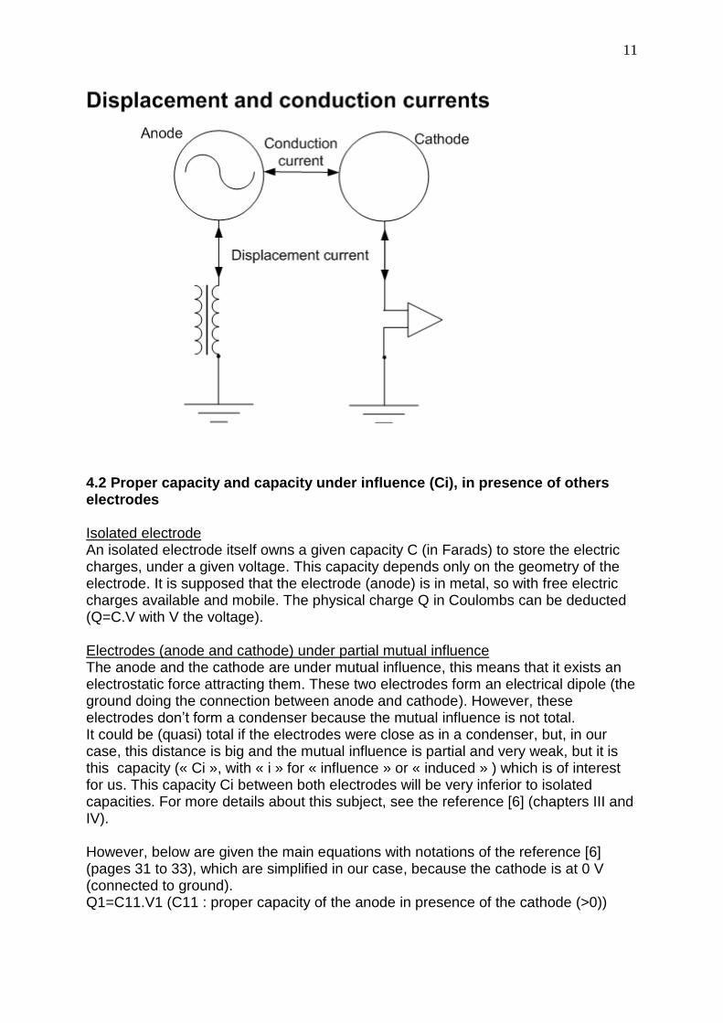
11

4.2 Proper capacity and capacity under influence (Ci), in presence of others electrodes Isolated electrode An isolated electrode itself owns a given capacity C (in Farads) to store the electric charges, under a given voltage. This capacity depends only on the geometry of the electrode. It is supposed that the electrode (anode) is in metal, so with free electric charges available and mobile. The physical charge Q in Coulombs can be deducted (Q=C.V with V the voltage). Electrodes (anode and cathode) under partial mutual influence The anode and the cathode are under mutual influence, this means that it exists an electrostatic force attracting them. These two electrodes form an electrical dipole (the ground doing the connection between anode and cathode). However, these electrodes don’t form a condenser because the mutual influence is not total. It could be (quasi) total if the electrodes were close as in a condenser, but, in our case, this distance is big and the mutual influence is partial and very weak, but it is this capacity (« Ci », with « i » for « influence » or « induced » ) which is of interest for us. This capacity Ci between both electrodes will be very inferior to isolated capacities. For more details about this subject, see the reference [6] (chapters III and IV). However, below are given the main equations with notations of the reference [6] (pages 31 to 33), which are simplified in our case, because the cathode is at 0 V (connected to ground). Q1=C11.V1 (C11 : proper capacity of the anode in presence of the cathode (>0))

12

Q2=C21.V1 (C21 : influence coefficient (negative capacity) between the anode and the cathode (<0)) Afterwards, it will be noted Ci=-C21, so Q2=-Ci.V1 V1=(1/C1).Q1 + (1/Cd).Q2 (C1 : capacity of the anode isolated in space (>0) and Cd a coefficient (negative capacity) depending on the geometry and the distance between electrodes) V2=0=(1/Cd).Q1 + (1/C2).Q2 (C2 : capacity of the cathode isolated in space (>0)) Determination of the Ci value For 2 spheres of respective radius R1 (for the anode) and R2 (for the cathode) and separated by a distance d, such that d>>R1 and R2, it can be shown that Ci tends to the following value : Ci=4*Pi* ε0*R1*R2/d.

Note : strictly speaking, the « influence coefficient » Cij is always negative and the capacity between electrodes Ci, equal to |Cij| is always positive.

It has to be noted that :

electrical charges on the cathode are inverted compared to those present on the anode,

the capacity of an isolated sphere of radius R1being valued as C=4*Pi* ε0*R1, it follows that Ci=C1*R2/d, C1 being the anode capacity (considered as isolated because at long distance from the cathode).

As any electrode tends to behave in an isotropic way at long distance, it follows that it can be considered an electrode of any shape as a sphere which center would correspond to the barycentre of electrical charges. In this case R (R1 or R2) would be considered as the characteristic dimension L of the electrode. For example , for a disk L=0.317 * the disk diameter, experimentally determined. Multiplasma (reference [7]) can be used, to determine Ci at a given distance.

Note : it is possible to change scale, as for example to interpret « mm » (base unit of Multiplasma) as cm or dm, but it will be necessary to apply a scale law (« law of similarity » ) (see the end of the Multiplasma handbook for details).

4.3 Electrical charge Q2 condensed on the cathode The charge Q2, condensed on the cathode, results from the capacity under influence Ci (Q2=-Ci.V1, with V1 the voltage on the anode). For example, for a system composed of two spheres (anode of radius R1 and cathode of radius R2, separated by a distance d), it is found : Q2=-4*Pi* ε0*R1*R2*V1/d (with ‘-‘ because the electrical charge is of opposite sign from the one condensed on the anode) Below, it will be found a screenshot of the Multiplasma program (reference [7]) showing the equipotentials between both electrodes :

on the left, an anode under the shape of a disk of diameter 10 cm and thickness 1 mm, supplied by 1000 V DC (direct current),

13

on the right, a cathode under the shape of a disk of diameter 5 cm and thickness 1 mm, connected to ground (so at 0 V) and separated from the anode by a distance of 30 cm.

In the bottom windows, it is successively found the charge on E1 (Q1=3.6582 E-9 C) and the one on E2 (Q2=-1.9100 E-10 C) then the capacities Cii and |Cij|. The one of interest is the influence capacity (Ci) between the electrodes Ci=|C12|=|C21|=0.1918 pF (or 1.9118 E-13 F). In this case, in can be noted that Ci=-Q2/V1 taking into the calculation uncertainties (the equipotentials and charge calculation being much more precise than the direct calculation of the capacities).

14

Of course, in our case, the transmitter will be supplied with an alternative current (AC) at a frequency « f » (of pulsation w=2Pi*f) and not in direct current, but this does not change the scope of the calculations. For example, the instantaneous charge on the anode can be expressed in the following way : Q1(t) = C11.V1.cos(w.t) with V1 the peak voltage on the anode. 4.4 Determination of the voltage (Vi) induced by the sole anode at cathode position Important : the cathode is not considered here as an electrode. Only its position is taken into account. It could also be considered that the cathode as isolated (not connected to ground), which comes to the same. Let’s suppose that the anode be a sphere of radius R1 raised at a voltage V1. It can be shown (using the sphere capacity) that the induced voltage in DC at a distance d is equal to Vi=V1*R1/d

Note 1 : the induction is supposed to propagate at the light speed. Nota 2 : in accordance with hypothesis taken in §4, it will be suppose that Vi and V1 have the same phase (to simplify, but this does not change anything in the principle).

For an electrode of any shape, R1 will correspond to the characteristic dimension L of the electrode (L=0.317*the disk diameter), with Vi= V1*L/d. It can be shown, using the Green reciprocity theorem (Reference [8] page 92) that Vi=(Q1-Q’1)*V1/Q’2. In this scope, one can use Multiplasma (reference [7]) to determine :

Q1 : the charge of the anode under voltage, alone (in single pole)

Q’1 : the charge of the anode under voltage, but with the cathode at 0 V under anode influence

Q’2 : the charge of the cathode at 0 V under influence of the anode Multiplasma (reference [7]) can also be used to directly to determine Vi at any distance along the z axis (horizontal). Below, on the screenshot, it can be seen that at z=+150 (cathode position), the induced voltage is equal to 104.9 V. It will be noted that the « field » around the disk tends to behave in an isotropic way at long distance, as for a sphere : the equipotentials seem to ellipses near the anode and to circles as soon as the distance from the anode increases.

15

16

4.5 Thévenin model of the “Cathode source” The general electrical model corresponding to the equations is given on the diagram below. Note that there is a voltage drop between anode and cathode due to the partial mutual influence.

The cathode can be seen as an electrode receiving energy from the upstream anode and delivering this energy on the load downstream. So the cathode is in the same time a receiver and a generator. The Thévenin model to determine is relative to the cathode seen from the « generator » point of view. It is thus necessary to determine 2 parameters : the open circuit voltage and the internal reactance :

The open circuit voltage of the “cathode” generator must be determined. Here it corresponds to the voltage Vi induced by the anode (and not V1). Indeed, if the cathode is isolated (or connected to ground via an infinite resistance), it will be submitted to the Vi voltage (cf. §4.4).

To determine the internal reactance Zi, it is enough to remove the load and to replace the generator by a short-circuit. In this case, from the load terminals, it remains Ci=-C21, so the internal reactance is the one given by Ci. The Thévenin diagram of the « Cathode source » is given in the next page.

Note : it is considered the input capacity and not the input resistance because in general the input resistance is widely superior to the input reactance, so the resistance can be neglected. For example, the digital voltmeter used for the tests has an impedance of 10 MOhms/100 pF in parallel. Now the reactance of the 100 pF capacity gives 178 Ko (at 8900 Hz), value very inferior to 10 MOhms.

17

According to the Ci and C values, it appears three different cases, presented below. Cc to Ci matching One can find to know what is the value Cc of the input capacity which permits to have the maximum of power on load level. It will be noted Zi=1/(j.Ci.w)=-j Xi with Xi= 1/(Ci.w) Ci and C form a capacitive bridge, so V/Vi=Ci/(Cc+Ci) After several calculations, it is found that the (reactive) available power P on Cc is equal to : P=Vi2.Ci2.Cc.w/(Ci+Cc)2 To find the ideal reactance, it is enough to derive P with respect to Cc then to equalize the result to 0. It will be found that Cc=Ci permits to match the maximum of power. This one is equal to Pmaximum=Vi2.Ci.w/4. It has been seen previously that for spheres, in the hypothesis of a long distance between anode and cathode :

Vi=V1*R1/d (R1: anode radius),

Ci=C1*R2/d (R2: cathode radius). Finally, it is founded that, in this case, Pmaximum=(V12 .R12.R2.C1.w)/d3 , with V1,R1,R2 et C1 independent from d. Given that any electrode tends to behave in an isotropic way at long distance (thus as a sphere), it follows that, in all cases, the maximum available power varies in 1/d3, if impedances are matched (Ci=Cc). Ci very inferior to Cc case In the general case, Ci is so much weak (quickly inferior to 0.1 pF) that Cc cannot be matched to Ci (case of the digital voltmeter used for the tests). It must be considered that Ci<<Cc. In this case, V/Vi=Ci/Cc and P=Vi2.Ci2.w/Cc. For spheres, it is found P=(V12 .R12.R22.C1.w)/d4 In this case, the maximum available power varies in 1/d4 (unfavorable case).

18

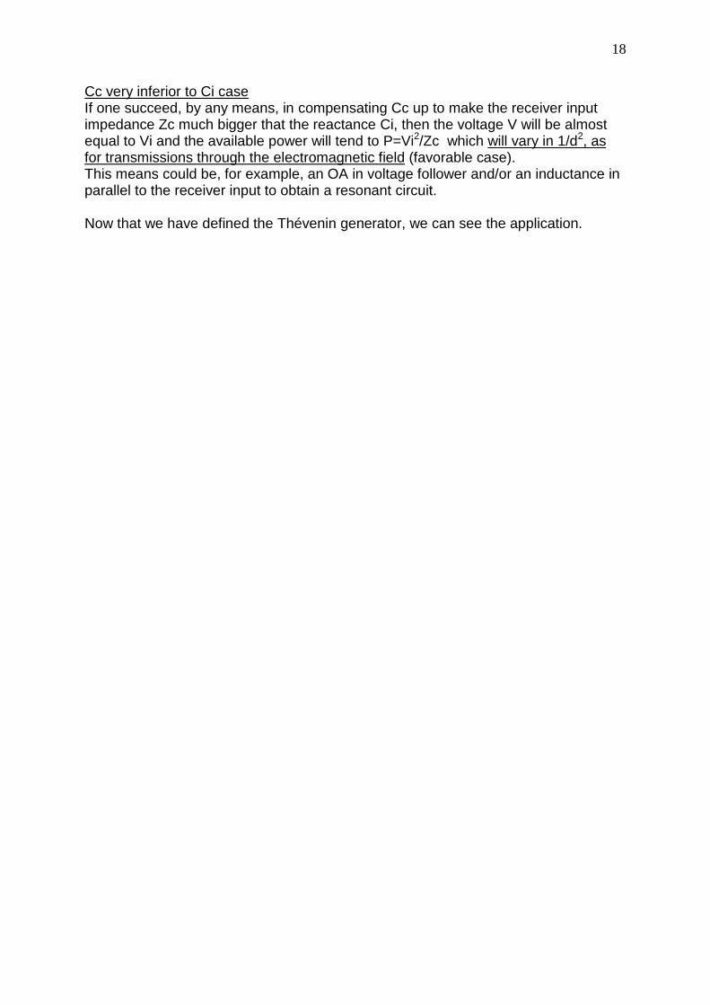
Cc very inferior to Ci case If one succeed, by any means, in compensating Cc up to make the receiver input impedance Zc much bigger that the reactance Ci, then the voltage V will be almost equal to Vi and the available power will tend to P=Vi2/Zc which will vary in 1/d2, as for transmissions through the electromagnetic field (favorable case). This means could be, for example, an OA in voltage follower and/or an inductance in parallel to the receiver input to obtain a resonant circuit. Now that we have defined the Thévenin generator, we can see the application.

19

5. Application 5.1 Principle diagram The author having at his disposal only one HF transceiver, tests could not be done on low Ham HF bands (let’s say from 135.7 to 1850 KHz). On the other hand, as he has at his disposal several PC equipped with a sound card, tests have been done on the 3 to 9 KHz band (which is not regulated) . Moreover, the 8.7 to 9.1 KHz band (called « Dreamer’s band ») seems to be an experimental band in several countries (see https://sites.google.com/site/sub9khz/). As a result of that, hereafter is what the author proposes.

20

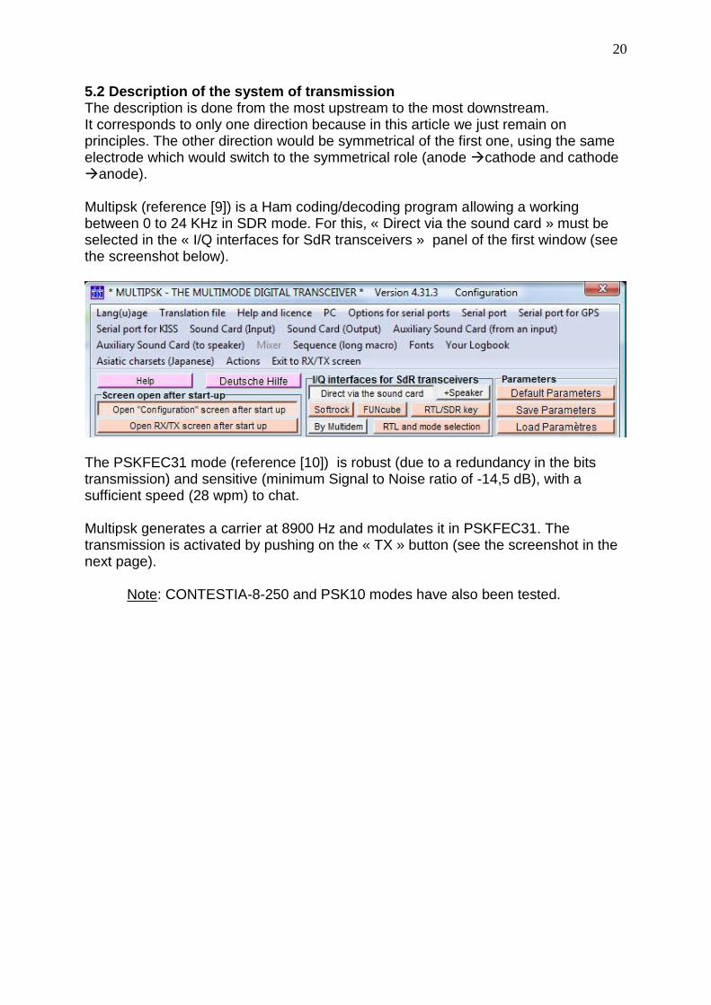
5.2 Description of the system of transmission The description is done from the most upstream to the most downstream. It corresponds to only one direction because in this article we just remain on principles. The other direction would be symmetrical of the first one, using the same electrode which would switch to the symmetrical role (anode cathode and cathode anode). Multipsk (reference [9]) is a Ham coding/decoding program allowing a working between 0 to 24 KHz in SDR mode. For this, « Direct via the sound card » must be selected in the « I/Q interfaces for SdR transceivers » panel of the first window (see the screenshot below).

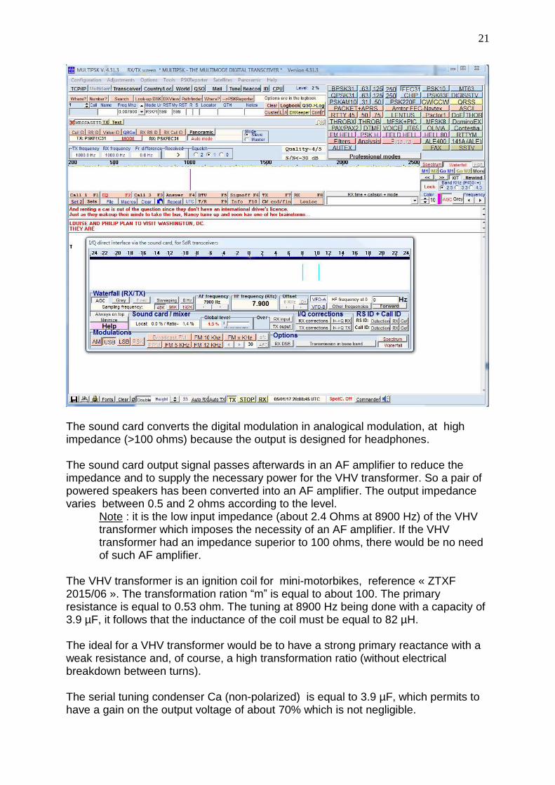
The PSKFEC31 mode (reference [10]) is robust (due to a redundancy in the bits transmission) and sensitive (minimum Signal to Noise ratio of -14,5 dB), with a sufficient speed (28 wpm) to chat. Multipsk generates a carrier at 8900 Hz and modulates it in PSKFEC31. The transmission is activated by pushing on the « TX » button (see the screenshot in the next page).

Note: CONTESTIA-8-250 and PSK10 modes have also been tested.

21

The sound card converts the digital modulation in analogical modulation, at high impedance (>100 ohms) because the output is designed for headphones. The sound card output signal passes afterwards in an AF amplifier to reduce the impedance and to supply the necessary power for the VHV transformer. So a pair of powered speakers has been converted into an AF amplifier. The output impedance varies between 0.5 and 2 ohms according to the level.

Note : it is the low input impedance (about 2.4 Ohms at 8900 Hz) of the VHV transformer which imposes the necessity of an AF amplifier. If the VHV transformer had an impedance superior to 100 ohms, there would be no need of such AF amplifier.

The VHV transformer is an ignition coil for mini-motorbikes, reference « ZTXF 2015/06 ». The transformation ration “m” is equal to about 100. The primary resistance is equal to 0.53 ohm. The tuning at 8900 Hz being done with a capacity of 3.9 µF, it follows that the inductance of the coil must be equal to 82 µH. The ideal for a VHV transformer would be to have a strong primary reactance with a weak resistance and, of course, a high transformation ratio (without electrical breakdown between turns). The serial tuning condenser Ca (non-polarized) is equal to 3.9 µF, which permits to have a gain on the output voltage of about 70% which is not negligible.

22

Note 1: a parallel tuning has no interest because the quality factor of the primary coil is too weak. Note 2 : the secondary impedance is so big that for the transformer, it is almost a working on an open circuit. Indeed, it can be determined the capacity of a disk of 270 mm (as anode) alone: 9.86 pF. So the impedance of this one is equal to Zs=1/(C.w)=1.8 Mohms. Even brought back to the primary Zp=1.8 E6/m2=180 ohms is negligible (“m” is the transformation ratio).

At the VHV transformer output, the maximum voltage is about 700 V RMS, so 1000 V peak. The anode and the cathode are, in fact, metal lids (used to cook). It is necessary to insulate the anode with a plastic film, to avoid to touch a surface at 1000 V.

Cautions At this level, it is not useless to remind here that the maximum of precautions must be taken against the risk of electrocution in VHV (gloves and insulation clothing…). It is necessary to check that all conductors of the VHV part are insulated. As a precaution, it must be considered that the breakdown voltage in air is equal to 1000 V/mm.

A high impedance input (here a CA3140 OA) is indispensable due to the high output impedance of the generator (cf. §4.5). Otherwise, the electric field 50 or 60 Hz is strong and, of course, present everywhere. It must be reduced at the maximum in the receiver. To do so, it has been added an input resistance R of 10 MOhms which limits the 50 or 60 Hz. The value of 10 MOhms has been fixed experimentally. It is this input resistance R at 10 MOhms which is going to, on the whole, fix the receiver input impedance (the one of the OA normally increases widely in voltage follower configuration).

Note : the author will test further (§6.4) if the OA input capacity (4 pF) really decreases in voltage follower configuration.

The CA3140 OA, configured in voltage follower, provides the signal under an output impedance of about 60 Ohms, which is sufficiently low. For more 50/60 Hz filtering, it is added, at the OA output, a coupling condenser Cf=2.2 nF which has a reactance of 8.1 KOhms at 8900 Hz, compatible with the microphone input impedance (10 to 50 KOhms). It will be found below the electronic diagram of the receiver.

23

This analogical signal is afterwards transmitted to the sound card microphone input (input impedance >=10 KOhms) which digitalizes the signal. Note that sound cards include an anti-aliasing filter which cuts frequencies above 24 KHz.

Note : the « ground » both for the transmitter as for the receiver is the electrical grid ground (which forms the return line).

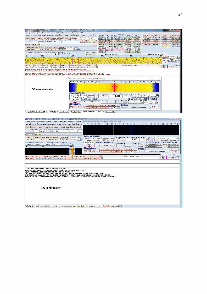
The digital signal is afterwards demodulated and decoded by Multipsk. The received message is displayed (it must correspond to the transmitted message). Hereafter, it will be found a picture and two screenshots showing the test equipment. On the left is the transmitter part and on the right the receiver part.

24

25

6. Tests and improvements in the course of tests 6.1 Available voltage and control of the law in 1/d4 Preliminaries As a first step, the author will show that, in the « Ci very inferior to Cc case » configuration (§4.5), it will be found an evolution in 1/d4. The author uses a digital voltmeter, so it can be considered that the previous Thévenin diagram (§4.5) is applicable with an input capacity Cc=100 pF. As V/Vi=Ci/Cc (§4.5), it follows that V=Vi.Ci/Cc. Previously, we have seen that for spheres, in the hypothesis of a long distance between anode and cathode :

Vi=V1*R1/d (R1: anode radius),

Ci=C1*R2/d (R2: cathode radius). So V=(V1*R1)/d*(C1*R2/d) = V1*R1*C1*R2/(Cc*d2) For standard electrodes, R1 and R2 can be replaced by their respective characteristic dimension. So the voltage measured on the terminals of the AO must vary in 1/d2 to show an evolution of the power in 1/d4. Test

Warning : measures done here are not laboratory ones, realized with certified equipment, according to a protocol, but measures done with amateur equipment without any protocol.

Multipsk is placed in « Tune » (transmission of a non-modulated carrier). It will be found an output voltage on the anode of about 577 V (“about” because the voltage fluctuates). Distance between electrodes (cm) Voltage (V) 31 8.85 50 3.7 80 1.28 100 0.73 120 0.53 150 0.4 As it can be seen, the voltage evolution follows a law in 1/d2. In fact, more precisely the voltage evolves according to Vi.Ci. 6.2 First tests in the configuration described in §5.2 Résults

26

Tests have been done at the maximum distance available on the author « experimentation table », i.e. 2,5 m. The limit to the PSKFEC31 transmission decoding depends first on the Signal to Noise ratio which must not be too much degraded (minimum : -14.5 dB) and moreover on the signal distortion, more or less important, generated by the transmission/reception chain. The main noise source is the 50 Hz or 60 Hz which pollutes the band in spite of the filters. In these conditions, amplifying the signal by the sound card « microphone » amplifier does not change anything, except slightly degrading the Signal to Noise ratio. The minimum voltage on the anode which permits a transmission without errors at 2,5 m in PSKFEC31 is 1 Volt RMS. So at 700 V RMS, the maximum range would be only about 2.5*√(700/1)=66 m Problems to take into account for tests

If the sound card output voltage is too strong, the AF amplifier BF distorts the signal and this one is no more decodable in PSKFEC31 even if the Signal to Noise ratio is very favorable. In fact, above a given power, the AF amplifier distorts the signal. This phenomena is much less sensitive in CONTESTIA-8-250 or even PSK10.

To do precise measures, it is preferable to shield wires with aluminum foil (or equivalent).

At high voltage on the anode (for example 700 Volts RMS), the PC close to the anode has failures (for example, the mouse no more reacts). It is the same problem as the HF feedback with transceivers transmitting. So it is necessary to move away the PC in transmission and to supply the anode with shielded cable with the shield connected to ground.

6.3 Second tests with different improvements Digital mode During the first tests, it has been noted that the CONTESTIA 8-250 and PSK10 modes are very efficient :

CONTESTIA 8-250 is sensitive (minimum Signal to Noise ratio= - 13 dB) and above all very robust due to a very strong redundancy,

PSK10 is not as robust as CONTESTIA 8-250 because there is none redundancy. On the other hand it is very sensitive (minimum Signal to Noise ratio= - 17,5 dB).

50 Hz or 60 Hz interferences To limit the 50/60 Hz interferences, the PC in reception has been supplied on its battery. There is no immediate improvement, except if the receiver chassis is disconnected from the ground, the receiver working in floating ground. In that case the level of interferences is reduced by a factor 3 (from the SdR indications of Multipsk). Note that there is no more connection between electric ground and the chassis of the equipment in the reception part. The configuration is no more a single

27

dipole « Anode/Cathode » but two dipoles «Anode-ground » and « Cathode/receiver chassis», but this does not change anything. It has been tried to supply the receiver with a 9 V battery. This gives only a weak advantage on the 50/60 Hz noise as the power pack transformer might be galvanically insulated. So, it is possible not to use the 9 V battery. The 50/60 Hz interferences having been very reduced, the sound card « microphone » amplifier has been used and adjusted on the +20 dB position, this to increase the signal level. Results The voltage level on anode becoming very weak, it has been measured the minimum voltage when no signal is transmitted. It has been found 0.035 V RMS. In these conditions, about the minimum voltage on the anode permitting a transmission without errors at 2,5 m is:

in CONTESTIA 8-250, this voltage is 0.051 Volt RMS . If the minimum voltage is considered, it is found √((0.051)2-(0.035)2)=0.037 V RMS. So at 700 V RMS, the maximum range would be about 2.5*√(700/0.037) = 344 m.

in PSK10, this voltage is 0.043 Volt RMS . If the minimum voltage is considered, it is found √((0.043)2-(0.035)2)=0.025V RMS. So at 700 V RMS, the maximum range would be about 2.5*√(700/0.025) = 418 m.

Maximum ranges (344 and 418 m) still remain weak. 6.4 OA test in voltage follower 6.4.1 Test without the R input résistance The OA CA3140 input impedance is 1.5 E12 ohms in parallel on a 4 pF capacity (4.5 MOhms at 8900 Hz). Theoretically in voltage follower, the input impedance is multiplied by G=(1+A) with A the open-loop gain. It can be estimated that the gain A is equal to the frequency at unity gain (3.7 MHz for the CA3140) which divides the frequency used (8900 Hz here). So A is equal to 415. The input capacity would hence pass from 4 pF to 4 pF/415 = 0.01 pF. It would be possible to work in the « Cc very inferior to Ci case » (cf. §4.5) and consequently with a power evolving in 1/d2, which would multiply the maximum range. So a test has been conducted by removing the 10 MOhms resistance R, the signal being directly applied to the OA input and the measure being taken at the OA output. It is found : Distance between electrodes (cm) Voltage (V) 31 0,88 50 0,43

28

80 0,13 100 0,100 120 0,046 150 0,03 It is noted that the voltage evolution unfortunately follows a law in 1/d2. Even worse, the voltage increases of 30% when the 10 MOhms resistance R is (re-)put in place. 6.4.2 Test after elimination of the parasitic capacity After searching a solution to this problem, it has been found that between the track connected to the OA input pin (+) and the ground, there had a parasitic capacity of 275 pF, which explained bad results. So, this pin (+) has directly connected to the cathode, without the resistance R nor the capacity of 470 nF. The residual capacity Cr (including the one of the OA in voltage follower) has been determined as being about 2,3 pF. Furthermore, to separate the 8900 Hz from the 50/60 Hz harmonics, the author has used Multipsk to measure the level on the band around 8900 Hz (in %). This level is homogenous to a voltage. It has been found the following levels (cf. following tables). In the first table, it can be seen that « N/N (at 20 cm) » follows the law in 1/d (« 20 cm/d ») up to about 80 cm, then, slowly, joins a law in 1/d2. This can be explained because the Ci capacity at d=20 cm is equal to 3.9 pF (and more for d<20 cm), it passes to 1 pF at 80 cm and finally to 0,4 pF at 2 m. Now the residual capacity (Cr) is about equal to 2.3 pF. So one passes from Ci>>Cr for d<<20 cm (law in 1/d, cf. §4.5) to Ci<<Cr at d>2 m (law in 1/d2, cf. §4.5). If the residual capacity Cr could be reduced down to 0 pF, the law followed would always been in 1/d. Distance between electrodes Level (L) L/ 20 cm/d (20 cm/d)2 (cm) (%) L (at 20 cm) 20 68.11 1 1 1 31 51.25 0.752 0.645 0.416 50 33.80 0.496 0.4 0.160 80 15.88 0.233 0.25 0.625 100 8.87 0.130 0.2 0.040 120 5.15 0.076 0.167 0.028 150 2.29 0.033 0.133 0.018 200 0.52 0.008 0.1 0.010 Below, it is shown the variation of Vi, Ci and Vi*Ci according to the distance. It can be shown that Vi and Ci follows, more or less, a law in 1/d and Vi*Ci a law in 1/d2.

29

Distance between electrodes 20 cm/d (20 cm/d)2 Vi/ Ci/ Vi*Ci/ (cm) Vi (at 20 cm) Ci (at 20 cm) Vi*Ci (at 20 cm) 20 1 1 1 1 1 31 0.645 0.416 0.691 0.668 0.462 50 0.4 0.160 0.443 0.424 0.188 80 0.25 0.062 0.281 0.267 0.075 100 0.2 0.040 0.226 0.214 0.048 120 0.167 0.028 0.188 0.179 0.033 150 0.133 0.018 0.151 0.143 0.022 200 0.1 0.010 0.113 0.108 0.012 An OA TL71, a LM741 and an OP27 have also been tested but less success. 6.5 Other possible improvement included the reception in differential mode and the electroscope List of the other possible improvements As we have now two dipoles («Anode-ground » and « Cathode/receiver chassis», we could think to improve either one or the other dipole. At this level, it can be reminded the formulas giving the received power P on the receiver (cf. §4.5) :

Cc=Ci : P=Vi2.Ci.w/4, varying in 1/d3

Ci<<Cc : P=Vi2.Ci2.w/Cc, varying in 1/d4

Cc<<Ci : P=Vi2/Zc , varying in 1/d2 To increase P, Vi and Ci must be increased and/or Cc must be decreased. For about Vi (voltage inducted by the anode, cf. §4.4), we can :

1. increase the voltage V1 on the anode, but caution on the electrocution risks, 2. increase the anode size: Vi is proportional to the anode characteristic

dimension, itself roughly proportional to the square root of its surface, 3. multiply the number of anodes (connected together).

For about Ci (influence capacity, cf. §4.2), we can :

1. increase the anode size or multiply the number of anodes (connected together),

2. increase the cathode size or multiply the number of cathodes (connected together),

Note : one could think to add a « reflector » connected to ground, just behind the anode to form a condenser, but this does not increase Ci.

For about Cc (input capacity, cf. §4.5), which reduced to the residual capacity Cr we can, to decrease (or even to cancel) its value, compensate it with a parallel resonance circuit (“trap circuit”):

1. either it is found the good value of inductance in parallel on the amplifier input but it will be necessary that the inductance be at a very high quality factor. This solution is not conceivable at 8900 Hz,

30

2. either a big capacity condenser (let’s say several nF, for example) is added in parallel to the amplifier input to be able to tune the whole with a weak inductance (on ferrite) of very high quality factor. This does not seem possible either at 8900 Hz, because the resistance of this trap circuit will not exceed the reactance of the 4pF of the OA.

For an OA, one can also improve the voltage follower which theoretically increases the input impedance and, so, decreases the AO input capacity. Perhaps supply voltages above +5/-5V (as used by the author) would decrease the residual capacity Cr. This case is, of course, the ideal case (but complicated one), because the maximum range will be widely increased due to the fact that all the voltage Vi is recovered. And even if the received power is negligible, the OA will give back all the necessary power to the signal.

Note 1 : if the OA input capacity could be completely compensated, then the CA3140 input impedance will pass to 1.5 TOhms (1.5 E12 Ohms) ! Note 2 : in this case, it is necessary to remove the resistance R of 50/60 Hz filtering, and only filter the 50/60 Hz downstream.

Reception in differential mode The author has tested a reception in differential mode, made according to the following diagram. It is hoped, ideally, that both noise sources (mainly 50/60 Hz) in common mode are going to cancel each other and that it will only remain the difference of voltage between cathodes #1 and 2, linked to their difference of distance compared to the anode. The Signal to Noise ratio might be appreciably increased.

31

The electronic diagram used is given below. The OA U2 and U3 are in voltage follower configuration. The outputs A and B of these OA drive the OA U4 in subtractor mode. The output of this OA (U4) is transmitted to the sound card input.

Note : this test has been done in the initial configuration (before elimination of the parasitic capacity). However, this elimination would not change not much here, because at 2 m it has been shown that the law is followed in 1/d2. In an ideal configuration where the residual capacity Cr would have been eliminated, it would be necessary to remove R1 et R2 from the following diagram. C6 et C9 could also been removed.

The comparison test is the following. The cathode #2 is at 2.5 m from the anode and the cathode #1 at 3.5 m from the anode. The cathodes are slightly laterally offset so as the cathode #2 does not hide the cathode #1. It is compared the normal reception done with the sole cathode #2 with the differential reception done with the cathodes #1 and 2. Test of the differential mode It is noted that the decoding in PSK10 starts on a voltage level about twice weaker in differential reception than in normal reception, which is positive.

32

Possible solution with an electrometer A possible solution would consist to use an electrometer vaccum tube to measure the very weak current issuing from the cathode. This thermoionic valve is called an “inverted triode” (the role of the plate (anode) and the grid being inverted). This apparatus would be able to measure currents down femtoA. However, it is aimed to continuous currents and not alternatives currents. Moreover the capacity of the control electrode is about several pF. This solution cannot be, a priori, envisaged. It would rather be necessary to envisage a solution directly implemented on the cathode. Solution with electroscope An electroscope is a mechanical electrometer. See Wikipédia with the key word « Electrometer » to see how it looks. Physically the two identical leaves at the same potential are loaded with the same electrical charge Q. The Coulomb force F which makes them repel is equal to F = 1/(4*Pi* ε0)*(Q/x)2, with x the distance between both leaves. According to the resistive force opposed by the spring (it’s a picture of course…), the charge Q value can be deduced. See the principle diagram below.

This concept could be directly applied to the cathode. Let’s imagine that this one is an electroscope. Both leaves, due to the anode electrostatic induction, are going to accumulate identical (and variable) charges according to the variable induced voltage Vi and the influence « capacity » Ci (§4.5). Let’s suppose that it could be possible to very precisely measure (at any time) the repulsion force F(t). So Q(t) would be deduced from F(t). Moreover, Q(t) is equal to Q(t)=Ci.Vi (§4.5) . As one knows that Ci and Vi are both proportional to the inverse of the distance, it follows that Vi can be extracted as being the square root of Q(t) (ignoring a constant factor), Q(t) varying in 1/d2. From Vi (varying in 1/d), it will be enough to manage this Vi value by the demodulator/decoder (the power in V2 will vary in 1/d2). It must be noted that an electroscope having a mechanical resonance around the transmitted frequency would be better. Of course, this apparatus does not exist…

33

7. Conclusion This type of digital transmission using the sole electric field, in the current state of what is available for amateurs, can permit links on several hundreds of m (cf. §6.3), but not beyond, except if an elevated voltage is used (which is dangerous) or if very large electrodes are used. For those for which such subject would have some interest, there are several possibilities of improvement :

on the reduction (see the quasi-complete elimination) of the amplifier input capacity (residual capacity Cr). Its resolution would permit to multiply the maximum range (cf. §4.5, §6.4.2 and §6.5), passing from an evolution of the received voltage in 1/d2 to an evolution in 1/d.

on the reception in differential mode which, if not increasing the signal level, increases the Signal to Noise ratio. The first positive test realized by the author (cf. §6.5) remains to be confirmed,

on the electrodes configuration. One could carry out simulations with Multiplasma (cf. [7]) or another equivalent soft,

on the possibility to transform the cathode in electroscope (cf. §6.5).

34

8. References [1] “Transmissions numériques magnétiques souterraines” by Bernard Lheureux (in French) http://www.tepex.fr/html/noteBL.html [2] « Apparatus for transmission of electrical energy » patent of 1900 by Nikola Tesla : http://www.mcnikolatesla.hr/wp-content/uploads/bsk-pdf-manager/81_00649621.PDF

[3] « Ondes électromagnétiques dans le vide » by Olivier Granier (in French): http://olivier.granier.free.fr/cariboost_files/PC-ondes-EM-vide.pdf [4] Patent WO 2007 107642 A1 « Device for transporting energy by partial influence through a dielectric medium » - Inventors : Patrick Camurati and Henri Bondar : http://www.google.fr/patents/WO2007107642A1?cl=en&hl=en [5] « Quelques remarques sur la transmission de l’énergie électromagnétique en champ proche » (in French) by H. Bondar and F. Bastien (PDF available on the Net) [6] “Cours d’Electrostatique-Electrocinétique” by Jonathan Ferreira (in French) (PDF available on the Net) [7] “Multiplasma 1.0” from the author (F6CTE) (in French and English): http://f6cte.free.fr/MULTIPLASMA_setup.exe [8] « The mathematical theory of electricity and magnetism » by Jeans (available on the Net) [9] “Multipsk 4.31.3” from the author (F6CTE) (basically in French and English but also in Spanish with an add-on): http://f6cte.free.fr/MULTIPSK_setup.exe [10] Description of the PSKFEC31 mode : http://f6cte.free.fr/PAPERS.ZIP