Wireless Sensor Networks - Network Coded Cooperative

IT 12 070

Examensarbete 30 hpDecember 2012

Wireless Sensor Networks - Network Coded Cooperative Communication

Design and Implementation

Nenghui Cui

Institutionen för informationsteknologiDepartment of Information Technology

mailto:[email protected]

Teknisk- naturvetenskaplig fakultet UTH-enheten Besöksadress: Ångströmlaboratoriet Lägerhyddsvägen 1 Hus 4, Plan 0 Postadress: Box 536 751 21 Uppsala Telefon: 018 – 471 30 03 Telefax: 018 – 471 30 00 Hemsida: http://www.teknat.uu.se/student

Abstract

Wireless Sensor Networks - Network CodedCooperative Communication

Nenghui Cui

This thesis is concerned with the design and implementation of a testbed for networkcoded cooperative communication (NC-CC) in IEEE 802.15.4-based wireless sensornetworks (WSNs). The work and test are based on Contiki 2.5 and sensor nodesZolertia Z1.In the testbed, a new network framework with large extensibility is provided, as wellas a basic realization of NC-CC. In our implementation, CC is realized as a Rimeprimitive in Contiki, while NC is inserted as a new layer between Rime and MAC toperform opportunistic coding. In this way the network stack of Contiki is extendedwhile still keeping the backward compatibility. Because of the lack of multicast in IEEE802.15.4 protocol and the contradiction of applying continuous overhearing onpower-constraint sensor nodes, new mechanisms called pseudo overhearing andpseudo multicast is proposed in our testbed.A configurable test program is also designed for the purpose of evaluation. Acombination of two senders, one relay and one destination is used as our networkmodel. Experiments show that all the designed functions work properly. But to berobust, more experiments under different models should be brought in the future. Amore detailed report on the experiments can be found in my project-partner YitianYan’s thesis.

Tryckt av: Reprocentralen ITCIT 12 070Examinator: Lisa KaatiÄmnesgranskare: Ping WuHandledare: Edith Cheuk-Han Ngai

Acknowledgements

I own my deepest gratitude to my family, without their support

I would never have had chance to study at Uppsala University,

not mention to start writing this thesis. Their endless love

gives me huge courage and faith in front of either study or life.

It also gives me great pleasure in acknowledging my

supervisor Edith Cheuk-Han Ngai and reviewer Ping Wu. Not

only because of their proper professional guidance all

through my thesis, but also thanks to Ngai’s happy smile the

magic power of which could always draw me away from

whatever-caused depressive mood, and thanks to Ping’s very

kind admonitions and correctness when I behaved too young.

Thanks to my project partner Yitian Yan. We shared the

longest time with each time during our theses. It might be our

most precious mutual memory in our lives.

I would also like to thank many of my friends who stayed with

me all the past year, sharing my happiness and sadness,

giving me power and hope. You made my life full of

splendidness.

I

Contents

List of Figures .......................................................................................................................... V

List of Tables .......................................................................................................................... VII

Glossary .................................................................................................................................. IX

Chapter 1. Introduction ..................................................................................................... 1

1.1 Background and Motivation ...................................................................................... 1

1.2 Challenges ................................................................................................................. 2

1.3 Our solution ............................................................................................................... 3

1.4 Delimitations and Assumptions ................................................................................ 4

1.5 Thesis Structure ......................................................................................................... 5

Chapter 2. Preliminaries .................................................................................................... 7

2.1 Wireless Sensor Networks......................................................................................... 7

2.2 Contiki ....................................................................................................................... 7

2.2.1 The network stack ............................................................................................ 8

2.2.2 Chameleon architecture .................................................................................. 8

2.2.3 Rime stack ........................................................................................................ 9

2.2.4 Packet attributes ............................................................................................ 10

2.2.5 Packet buffer .................................................................................................. 12

2.2.6 Announcement layer...................................................................................... 13

2.2.7 Radio duty cycle (RDC) ................................................................................... 14

2.3 Zolertia Z1................................................................................................................ 14

2.4 Cooperative Communication .................................................................................. 15

2.4.1 Overview ........................................................................................................ 15

2.4.2 Strategies of cooperation............................................................................... 16

2.4.3 The overhearing ............................................................................................. 17

2.4.4 Relay selection ............................................................................................... 18

II

2.5 Network Coding ....................................................................................................... 19

2.5.1 Overview ........................................................................................................ 19

2.5.2 Coding Algorithms .......................................................................................... 20

Chapter 3. Design Considerations and Related Works .................................................... 21

3.1 Preconditions .......................................................................................................... 21

3.1.1 The network environment ............................................................................. 21

3.1.2 Other requirements ....................................................................................... 21

3.2 Cooperative Communication .................................................................................. 22

3.2.1 Positioning...................................................................................................... 22

3.2.2 Pseudo overhearing ....................................................................................... 23

3.2.3 Target packets ................................................................................................ 23

3.2.4 Relay determination ...................................................................................... 24

3.2.5 Relay strategy ................................................................................................. 24

3.3 Network Coding ....................................................................................................... 25

3.3.1 Positioning...................................................................................................... 25

3.3.2 Overhearing ................................................................................................... 25

3.3.3 Coding targets ................................................................................................ 25

3.3.4 Pseudo multicast ............................................................................................ 26

3.3.5 Packets selection ............................................................................................ 26

3.3.6 Response mechanism .................................................................................... 26

3.3.7 Buffer management ....................................................................................... 27

Chapter 4. Design and implementation ........................................................................... 29

4.1 Overview ................................................................................................................. 29

4.2 The CC Primitive ...................................................................................................... 30

4.2.1 General process ............................................................................................. 30

4.2.2 Announcements ............................................................................................. 31

4.2.3 Neighbour table ............................................................................................. 31

4.2.4 Relay selection ............................................................................................... 32

4.2.5 Packet header ................................................................................................ 32

III

4.2.6 The CC primitive ............................................................................................. 33

4.2.7 Configurable parameters ............................................................................... 34

4.2.8 Overheads ...................................................................................................... 34

4.3 The Networking Coding Layer ................................................................................. 35

4.3.1 Overview ........................................................................................................ 35

4.3.2 Work flow ....................................................................................................... 35

4.3.3 Buffers ............................................................................................................ 36

4.3.4 Packet header ................................................................................................ 36

4.3.5 Packet length ................................................................................................. 38

4.3.6 Encoding ......................................................................................................... 39

4.3.7 Decoding ........................................................................................................ 39


4.3.9 Overheads ...................................................................................................... 40

Chapter 5. Experiments and Evaluation .......................................................................... 42

5.1 The Test Program .................................................................................................... 42

5.1.1 Feature list ..................................................................................................... 42


5.2 Overview of results ................................................................................................. 44

5.3 Experiment 1: unicast & CC comparison ................................................................. 44

5.4 Experiment 2: CC & NC-CC comparison .................................................................. 48

Chapter 6. Conclusion & Future works ............................................................................ 50

6.1 Conclusion ............................................................................................................... 50

6.2 Future work and possible optimization .................................................................. 50

Bibliography .......................................................................................................................... 52

Appendix A. The packet attributes available in Contiki ................................................. 55

Appendix B. Configuration file for test program ........................................................... 56

B.1. Original configuration file ................................................................................... 56

B.2. Custom configuration file ................................................................................... 56

B.3. Our configuration file ......................................................................................... 56

IV

Appendix C. Disabling address filtering in RDC layer ..................................................... 58

C.1. The original source code ..................................................................................... 58

C.2. Disable the address filtering to enable overhearing .......................................... 58

Appendix D. Configuration dictionary of test program ................................................. 59

Appendix E. The source-code list of our testbed .......................................................... 61

E.1. MAC layer ........................................................................................................... 61

E.2. NC layer* ............................................................................................................. 61

E.3. CC primitive* ...................................................................................................... 61

E.4. Test program* .................................................................................................... 61

V

List of Figures

Figure 1.1 the butterfly model of NC-CC ................................................................................. 2

Figure 1.2 the network model of NC-CC ................................................................................. 4

Figure 2.1 sample of wireless sensor networks ...................................................................... 7

Figure 2.2 the network stack of Contiki, in comparison of TCP/IP model .............................. 8

Figure 2.3 general work flow of Chameleon ........................................................................... 9

Figure 2.4 the structure of Rime stack .................................................................................. 10

Figure 2.5 a bit-optimized Rime header of a multihop channel (from 12.0 to 16.0, captured

on 16.0)......................................................................................................................... 11

Figure 2.6 the packet buffer for incoming packets ............................................................... 12

Figure 2.7 the packet buffer for newly generated packets ................................................... 13

Figure 2.8 the header priority in packetbuf of Contiki .......................................................... 13

Figure 2.9 architecture of announcement layer ................................................................... 14

Figure 2.10 Zolertia Z1 .......................................................................................................... 15

Figure 2.11 spatial diversity of Cooperative Communication ............................................... 16

Figure 2.12 data flow of direct transmission ........................................................................ 18

Figure 2.13 the concept of Network Coding ......................................................................... 19

Figure 2.14 a typical usage of network coding...................................................................... 20

Figure 4.1 the network stack with NC-CC implemented ....................................................... 29

Figure 4.2 the CC position as a channel in Rime stack .......................................................... 33

Figure 4.3 the place of NC header ......................................................................................... 37

Figure 4.4 four kinds of NC headers for different packets .................................................... 38

Figure 4.5 the length of packet encoded .............................................................................. 39

Figure 5.1 the RSSI value of unicast detected at the receiver side ....................................... 45

VI

Figure 5.2 the RSSI value of CC detected at the SINK side .................................................... 46

Figure 5.3 the RSSI value of packets from relay, detected at the SINK side ......................... 47

Figure 5.4 the RSSI value of packets from sender, detected at the SINK side ...................... 47

Figure 6.1 one optimization of the design of NC layer ......................................................... 51

VII

List of Tables

Table 2.1 the attribute-list of multihop primitive ................................................................. 11

Table 4.1 an example of neighbour table ............................................................................. 31

Table 5.1 Experiment Parameters of Comparing CC’s performance with unicast’s ............. 45

Table 5.2 Experiment Parameters of Comparing NC-CC's performance with CC’s ............... 48

Table 5.3 results of indoor experiment of comparing NC-CC with CC (power: 0dBm) ......... 48

Table 5.4 results of outdoor experiment of comparing NC-CC with CC (power: 0dBm) ...... 49

Table D.1 configuration dictionary of test program ............................................................. 59

IX

Glossary

CC Cooperative Communication

NC Network Coding

NC-CC Network Coded Cooperative Communication

WSN Wireless Sensor Network

E-Sender End-side Sender (the same meaning with original sender)

E-Receiver End-side Receiver (the same meaning with final receiver)

PID Packet ID

HDR Header

RSSI Received Signal Strength Indication

RDC Radio Duty Cycle

1

Chapter 1. Introduction

This chapter presents an introduction to the thesis, including the background and motivation of

the project and a brief summary of our solution. It starts with a discussion on the significant

improvement on the performance of wireless sensor networks (WSNs) by employing CC and NC

individually, and also the current achievements by combining them together. Then an

implementation of NC-CC on low-power WSNs is motivated, together with an analysis of

challenges we are facing with. After that, as our solution, a primitive design and implementation

of WSNs-based testbed is proposed shortly. Finally we claim some delimitation of our work and

also the structure of the following chapters.

1.1 Background and Motivation

In WSNs, due to the limits of sensor nodes’ size, weight, cost, and etc., some performance

problems like energy efficiency, reliability, latency, throughput, and etc. have been deemed as

the main challenges in this area [1]. Extensive researches have shown that cooperative

communication (CC) [2-4] and network coding (NC) [5] are effective in enhancement of the

performance of WSNs. Moreover, the possibility of combining these two emerging technologies

have also been talked intensely [6, 7] and many solutions have been proposed in recent years

[8-13].

CC has been proved to be effective on bringing some multiple-input multiple-output (MIMO)

benefits to WSNs that consist of single-antenna nodes. However, one drawback of CC is that it

brings some overheads due to the introduction of extra packets, which in turn may aggravate

the interference in wireless environments. NC, as a technology which can improve the network

throughput by reducing the transmitting packets, can be used as a good remedy to this

weakness.

The combination of CC and NC, which we called network coded cooperative communication

(NC-CC) here, theoretically should bring lots of benefits to WSNs such as space diversity,

interference reduction, and other benefits that only MIMO systems could have without bringing

heavy congestion to the network.

One typical combination of the two technologies is the butterfly model [5, 9] (Figure ), where

NC and CC work together to reach a maximal benefit of both spatial diversity and less

transmissions. In this model, P1 and P2 are two separate packets from node A and B

respectively to be sent to both nodes E and F (multicast). By using relay nodes C and D, both E

and F can gain spatial diversity but in regular transmissions it would cost two timeslots to

transmit P1 and P2 from C to D and another two timeslots from D to E and F. By applying

Chapter 1: Introduction

2

network coding on node C and D, transmissions are half reduced while keeping the benefits

brought by CC.

However, most of the practical works of CC and NC are based on 802.11 networks like the

widely talked CoopMAC for CC [14-17] and COPE for NC [18, 19]. The combination of NC-CC is

still on the theoretical stage and for other networks like cellular network [20] or 802.11 wireless

LANs [8, 9, 21, 22]. Moreover, most of the discussion is on physical level [7] like amplify-and-

forward and decode-and-forward. In 802.15.4 based WSNs, some roots that many theories

based on like multicast and overhearing become not easy anymore, and each consideration can

be even more sensitive by WSNs’ nature of consisting of tiny-size resource-constraint sensor

nodes. In such low-rate wireless environment, problems existed in regular wireless networks

like interference and signal fading, can be even more significant that many existing mature

protocols and architect cannot be usable in the new environment.

Although still a few works like [23] have been carried out on analysing the feasibility of applying

NC-CC on such low-rate WSNs, however, no real implementations have been given to evaluate

theoretical algorithms or other assumptions due to the lack of a suitable testbed. A testable,

easily configurable framework is urgently needed in order to make further step in this area.

1.2 Challenges

Although the work on 802.11-based wireless networks has gained lots of progress in theoretical

and practical aspects, 802.15.4-based wireless networks are very different and thus lots of work

on 802.11-based networks cannot be directly used.

A B

C

D

E F

P1 P2

P1 ⊕P2

P1 ⊕P2

P1 P2

P1, P2 P1, P2

Figure 1.1 the butterfly model of NC-CC

3

In 802.15.4-based wireless networks, some specific considerations are put on the top priority

when doing the design, such as the power consumption, the weak calculation capability and the

number of antennas. Functions like overhearing should be avoided or reduced as much as

possible. Too many packets will have significant impact on signal interference so protocols like

TCP/IP will not be suitable to put on such low-rate WSNs. Some features are innately missing in

802.15.4 like multicast, which is an essential part of many network coding solutions on 802.11-

based wireless networks so the whole structure of them need to be re-considered if someone

wants to move them to low-rate WSNs.

To conclude, there are still a bunch of details to consider when implementing a workable

testbed even there are many excellent examples to reference. Some ideas might be borrowed

but no existing solutions could be directly used without change. Therefore the structure of such

testbed is actually designed from zero. And the implementation on a specific platform is totally

new in this area.

1.3 Our solution

In this paper, we aim at the realization of a testbed for network coded cooperative

communication (NC-CC) in low-rate WSNs, using Zolertia Z1 wireless sensors [24] and Contiki

which is an open source operating system [25]. To this end, we extended the existing network

protocol stack of Contiki with the two technologies transparently applied. To be specific, we

inserted a new layer transparently between MAC and Rime layer for dealing with network

coding and extended the Rime primitives to support cooperative communication.

The new network framework is aim to be used as a test-bed for all the researchers who are

focus on either CC or NC or the combination of the two on low-rate WSNs. It is backward

compatible with the legacy 802.15.4 system. By using this testbed, one can easily apply new

algorithms into experiments and get the results in a practical environment, which is significantly

meaningful to both theoretical researches and practical applications development in the future.

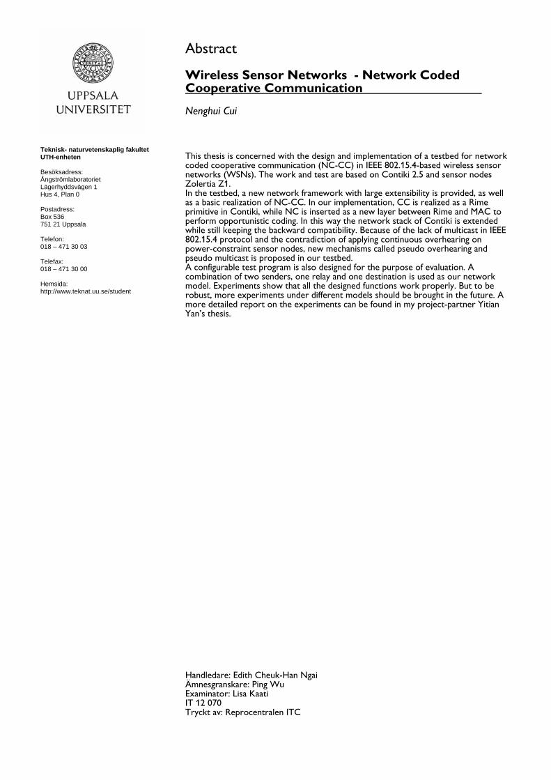
The model we use for NC-CC is described as Figure 1.2. At least two sender nodes are required

for network coding to take effect. In the figure they are marked with Sender A and Sender B.

Relay is an intermediate node selected to route when direct transmission may lead to worse

quality. Relay will opportunistically code several packets together, like as in the figure P1 and P2

are XOR-coded as one packet. Sink is a special sensor node used for collecting sensor

information from other nodes, usually equipped with a continuous power supplier and doesn’t

have to send out sensor information itself. In our model all the packets should make Sink as the

final receiver. The relay itself may also have sensor information to send in the reality. But here

as to simplify the model, we assume that relays are only used to forward packets.


4

The model above is a basic demonstration and can be adjusted for specific purposes. For

example, relay candidates can be more in order to test the relay selection algorithm. In our

implementation we select the ‘best’ relay based on the RSSI value, which will be talked in the

following chapters. Senders can be either single when NC is not enabled, or more than two in a

complicated network.

The detail of experiments by using this model will be talked on Chapter 5. The design of our

testbed will be explained in Chapter 3 and Chapter 4.

1.4 Delimitations and Assumptions

This thesis is intended to realize testbed of NC-CC in an 802.15.4-based WSN using Contiki

operating system. The focus will be put on the design and implementation of a workable

software architect, rather than the comparison of algorithms of CC or NC. The concrete

algorithm can be changed for different purposes of research. And it is our testbed that will

provide a much easier way to do such change so as to reduce the cost of implementing the

whole structure each time people want to test a specific theory. The testbed is far to a complete

perfect solution; instead it’s an initial work with a large space of improvement in the future.

To provide such a runnable testbed with easy configuration so that others can insert their own

algorithms or design ideas with minimal modification and evaluate it under a real environment,

as we can see in the following chapters, there are too many details to consider, each of which

could be a large topic. We will leave them as further work to other researchers who are

interested in. Here we list some delimitations of our implementation. The choice of each may

not be the perfect but it’s neither where our focus lies.

a. Technically WSNs are not limited to use 802.15.4 or other specifications. In this paper we

only consider those WSNs with 802.15.4 specification used. In the following chapters, when

we say WSNs, we are referring 802.15.4-based WSNs if not particularly specified.

Sender A

Sink

Sender B

Relay

P1

P2

P1 (overhear)

P2 (overhear)

P1 XOR P2

Figure 1.2 the network model of NC-CC

5

b. We use Contiki 2.5 as the target operating system on sensor nodes. There are many other

choices like TinyOS but again we would like to leave the chance to others. And up to now

Contiki has already published version 2.6 during the time of our working. We haven’t tested

our implementation under the newest version but theoretically it should have no problem.

Here we only talk about Contiki 2.5 all through the paper. When we say Contiki in the

following sections, we mean Contiki 2.5 if in a version-sensitive context.

c. We use Zolertia Z1 as our sensor nodes in experiments. It could be different results if one

uses other nodes for testing, since some performance may have large relationship with

hardware. Here we just compare the performance on the software level.

d. In our model as Figure 1.2, we assume that there are only at most two hops in the whole

transmitting route and such model is tested to be workable. But in the design we try to

make it as extensible as possible. The experiments are executed under the model as Figure

1.2. Other models with more hops could also work well or with a little bit adjustment but

there’s no promise for that.

e. In order to simplify the model, for easier comparison in the experiments, we assume the

relay doesn’t send data itself. Instead it only forwards packets from others when needed.

The model could still work if one makes relay to send data packets of its own, but the

performance may be largely different with what we evaluated in the experiments. A

possible bad result in that case doesn’t mean the overturn of our testbed; instead some

adjustment or improvement should be applied for that scenario.

f. In our model as Figure 1.2, the node called SINK is a special node whose purpose is to

collect data from other nodes. It doesn’t send data packets to any nodes. In some cases it

may send control packets or other necessary packets to make sure the model works. In our

model, it is the only mutual destination for all data packets. And we assume that a SINK

node should have continuous power supply instead of regular battery.

g. Some parts of our implementation, like the support of Z1, could be impacted by a third

force as the authors are continuously working on the improvement of Contiki. It is not

something under our control, and this is why we design our modules with very low-

coupling and try our best not to change the original source code.

1.5 Thesis Structure

In the following section, first we present a few preliminaries (Chapter 2) for understanding the

whole thesis.

Then in Chapter 3 we point out the main challenges we met while designing our testbed, and

the current research status for each issue, e.g., what others have done and how they contribute

to the progress of this area, and followed with how we thought about them.


6

In Chapter 4, we explain the detail of our design and how each part integrates together,

followed by the experiments and analysis we did (Chapter 5).

Chapter 6 presents the conclusion and some possible improvement that could be made in the

future.

7

Chapter 2. Preliminaries

2.1 Wireless Sensor Networks

A typical wireless sensor network (WSN) is made up of several sensor nodes, each equipped

with several specific sensors and antennas.

Sensor nodes are usually in small size and used outdoors. Therefore the power consumption is

always a big concern for both hardware and software development, which lead to the result of

weaker CPU, (usually) single antenna, and all kinds of software design for saving powers. Several

operating systems are specially designed for such power-constraint devices, like TinyOS [26] and

Contiki [25]. IEEE 802.15.4 [27] is such a standard that considered for low-rate wireless

networks, followed by many famous specifications such as ZigBee.

2.2 Contiki

Contiki is a lightweight and flexible operation system for memory-constrained networked

sensors, developed by Swedish institute of computer science (SICS) [25]. It uses a lightweight

event-scheduler in the kernel, leaving the pre-emptive multi-threading feature as an optional

library for applications. In [25] the details of Contiki like dynamic loading and replacement of

programs and services are introduced. But here we will only focus on thesis related knowledge,

mostly are network-based like the adaptive communication architecture of Contiki called

Chameleon [28], the Rime network stack [29], and radio duty cycles [30].

Most of the following introductions are based on the analysis of Contiki’s source code, as well as

published papers and some webpages. Contiki is implemented in the C language [25].

Figure 2.1 sample of wireless sensor networks

Chapter 2: Preliminaries

8

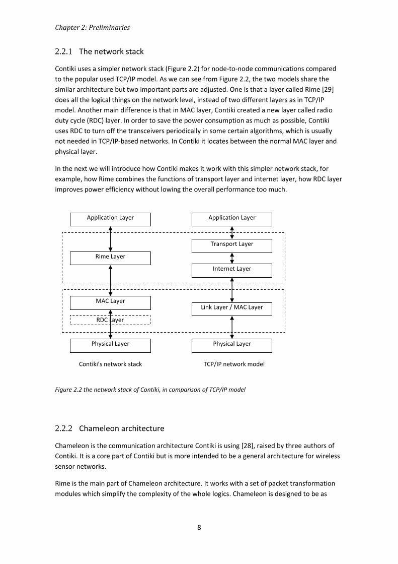
2.2.1 The network stack

Contiki uses a simpler network stack (Figure 2.2) for node-to-node communications compared

to the popular used TCP/IP model. As we can see from Figure 2.2, the two models share the

similar architecture but two important parts are adjusted. One is that a layer called Rime [29]

does all the logical things on the network level, instead of two different layers as in TCP/IP

model. Another main difference is that in MAC layer, Contiki created a new layer called radio

duty cycle (RDC) layer. In order to save the power consumption as much as possible, Contiki

uses RDC to turn off the transceivers periodically in some certain algorithms, which is usually

not needed in TCP/IP-based networks. In Contiki it locates between the normal MAC layer and

physical layer.

In the next we will introduce how Contiki makes it work with this simpler network stack, for

example, how Rime combines the functions of transport layer and internet layer, how RDC layer

improves power efficiency without lowing the overall performance too much.

Figure 2.2 the network stack of Contiki, in comparison of TCP/IP model

2.2.2 Chameleon architecture

Chameleon is the communication architecture Contiki is using [28], raised by three authors of

Contiki. It is a core part of Contiki but is more intended to be a general architecture for wireless

sensor networks.

Rime is the main part of Chameleon architecture. It works with a set of packet transformation

modules which simplify the complexity of the whole logics. Chameleon is designed to be as

RDC Layer

Application Layer

Rime Layer

MAC Layer

Physical Layer

Application Layer

Transport Layer

Link Layer / MAC Layer

Physical Layer

Contiki’s network stack TCP/IP network model

Internet Layer

9

adaptive as possible so as to separate the connection of different protocols. The detail of each

module will be introduced in the following sections.

The general work flow can be illustrated as Figure 2.3.

2.2.3 Rime stack

Rime stack is the main part of Chameleon. It is a lightweight layered communication stack for

sensor networks [29], locating between MAC layer and application layer.

Rime is designed to simplify the implementation of protocols in WSNs. It functions by providing

different kinds of communication primitives, like anonymous best-effort broadcast (abc),

identified sender best-effort broadcast (ibc), unicast abstraction (uc), reliable unicast (ruc), best-

effort multihop unicast (mh) and etc. (as listed in Figure 2.4)

These primitives are designed as many thin reusable modules so that other primitives can be

easily extended and more complex protocols can be easily set up on top of these primitives

(Figure 2.4).

Different Applications

Different Communication Primitives

Header transformation modules

Different MAC protocols

Rime stack

Figure 2.3 general work flow of Chameleon


10

Not like traditional layered communication architectures which were found too restrictive for

sensor networks [31], Rime designs each primitive-layer with high-level abstractions by taking

advantage of communication abstractions for distributed programming [32].

The Rime stack largely simplifies the implementation of protocols above primitives. The price is

a bit extra memory footprint. A preliminary evaluation is given in [29] showing that although

each primitive and each connection will have a small increase in the memory consumption, the

new implementation of complex protocols could have large decrease of both code lines and

memory footprint. The paper expects that in the future the overall resource consumption could

be better by using Rime stack.

2.2.4 Packet attributes

Chameleon separates the logic of different protocols/primitives and the low-level dealing of

packet headers [28] by using packet attributes.

Each communication primitive in Rime stack doesn’t need to handle the details of packet

headers like alignment or byte ordering. Instead, they simply keep a list of what kind of

attributes should appear in their headers and set the values before passing to lower layers. A

header transformation module will do the rest of things.

abc

Lower layer

ibc

uc

mh

Other primitives like stubborn ibc,

stubborn uc, reliable uc, unique abc,

unique ibc, best-effort multi-hop

flooding and etc.

Communication

primitives

Upper layer

Complex protocols like collect, mesh, routing, and etc.

Figure 2.4 the structure of Rime stack

11

Contiki provides a list of attributes name as enumerated type (see “Appendix A:

The packet attributes available in Contiki”). Addresses are also been treated as special types of

attributes. What each communication primitive or protocol has to keep is just the names of

attributes they want to have in headers. And those attributes, together with the channel

number of each primitive/protocol, form the content of Rime header.

Take multihop as an example. The attribute-list after expending is listed in Table 2.1. Each of

them should be set a correct value before passing to header transformation module. The

module will then get all the needed values from two global structures according to this

attribute-list, and put them bit by bit (by default chameleon_bitopt is used as the header

transformation module which does bit-optimization for headers) after the channel number.

Now a multihop channel numbered 135 wants to set up a connection from node 12.0 to node

16.0. Since there’s no third node, the packet will be directly sent to final receiver 16.0. The

packet header we detected on 16.0 can be explained by Figure 2.5. In Rime,

PACKETBUF_ADDRSIZE is two bytes.

Table 2.1 the attribute-list of multihop primitive

Type of attribute Size of attribute Description

PACKETBUF_ADDR_ESENDER PACKETBUF_ADDRSIZE The address of E-Sender

PACKETBUF_ADDR_ERECEIVER PACKETBUF_ADDRSIZE The address of E-Receiver

PACKETBUF_ATTR_HOPS PACKETBUF_ATTR_BIT * 5 The number of hops

PACKETBUF_ADDR_RECEIVER PACKETBUF_ADDRSIZE The address of receiver

PACKETBUF_ADDR_SENDER PACKETBUF_ADDRSIZE The address of sender

However, not all attributes are usable in Rime headers. There are actually three kinds of packet

attributes. By the difference of survival time, Contiki categorize them into three scopes [28]

(check “Appendix A” for detail categories):

10000111 (0x87) 00000000 (0x0)

00001100 (0xc) 00000000 (0x0)

00010000 (0x10) 00000000 (0x0)

00001000 (0x8) 10000000 (0x80)

00000000 (0x0) 01100000 (0x60)

00000000 (0x0)

Channel number,

here it’s 135

E-Sender, 2 bytes,

here it’s 12.0

E-Receiver, 2

bytes, 16.0

Number of

hops, 5 bits

Receiver, 2 bytes,

here it’s 16.0 Sender, 2 bytes, here it’s 12.0 The last 3 bits are just empty

Figure 2.5 a bit-optimized Rime header of a multihop channel (from 12.0 to 16.0, captured on 16.0)


12

a. Scope 0. Local information, only available within the node.

b. Scope 1. Information between two neighbours. Often used by MAC or lower layers. Lost

after one hop transmission.

c. Scope 2. End to end information. Often used by Rime or higher layer. Keep alive until the

final destination received.

2.2.5 Packet buffer

Buffer management is also an important part of Chameleon architecture, in which it is also

called Rime buffer [28]. In Contiki they use one global structure to store a full-length packet,

either it’s incoming or outbound. The structure is named packetbuf in Contiki with a fixed length,

by default 176 bytes. Headers and data part are separated in two ways, depends on the flow

direction of packet:

For incoming packets, the whole packet is put in the later 128 bytes area of packetbuf (Figure

2.6).

For newly generated outbound packets, the management of packet buffer is different. The first

48 bytes are actually reserved for headers. But for incoming packets, we don’t know the length

of header before buffering and analysing it. If the same packet is to be sent out again, for

example, when to be forwarded, again we don’t know how large the new header could be so as

the overflow may happen if we put the packet from the first byte in the beginning. Fortunately

we don’t have to worry about headers if we are about to send out our own packets, since there

are actually no physical headers when data are ready. Later headers will be formatted by

header transformation module from back to front like Figure 2.7 says.

48 Bytes 128 Bytes

HDR DATA

Figure 2.6 the packet buffer for incoming packets

13

When adding headers in packet buffer, the priority goes with the packet flow, from application

layer to physical layer. Each layer maintains its own header, adding it in front of other headers

before passing to lower layers, and remove it before passing to upper layers when a packet

receives (Figure 2.8). There are some APIs provided by Contiki for each layer to easily get the

location where they should add or remove their headers. Although the buffer management is

different for different cases, the APIs are unified and used as the same.

Figure 2.8 the header priority in packetbuf of Contiki

2.2.6 Announcement layer

Announcement is a service provided by Contiki for exchanging neighbour information, and is

especially optimized for low power WSNs with radio duty cycles [33]. It provides a unified mean

to broadcast extra information for all running protocols (Figure 2.9).

48 Bytes 128 Bytes

HDR DATA

Figure 2.7 the packet buffer for newly generated packets


14

2.2.7 Radio duty cycle (RDC)

RDC is also a very important part in Contiki. In different with 802.11-based networks, 802.15.4-

based networks take much more concern on power consumption when designing protocols.

Under this principle, radio transceivers should be off as much as possible to avoid unnecessary

listening. This brings the motivation of the design of radio duty cycle (RDC).

Over years many RDC mechanisms have been brought out [34], such as B-MAC [35], S-MAX [36],

X-MAC [37], BoX-MAC [38] and etc. Contiki provides several implemented RDC drivers like

ContikiMAC, X-MAC, compatibility X-MAC (CX-MAX), low-power probing (LPP), and Null-RDC

[30].

ContikiMAC is the default mechanism in Contiki tailored for the 802.15.4 radio and the CC2420

radio transceiver. It is announced to have very good power efficiency by keeping the nodes

sleep for 99% of the time while keep communicating within networks [30, 39]. To ensure an on-

time wake-up each time, ContikiMAC uses the Contiki real-time (rtimer) to set the call-back

schedule function which runs as a protothread [40].

However, because of the usage of very strict wake-up intervals, ContikiMAC requires to turn off

the overhear function in order to work properly. That could cause problem when implementing

CC and NC.

2.3 Zolertia Z1

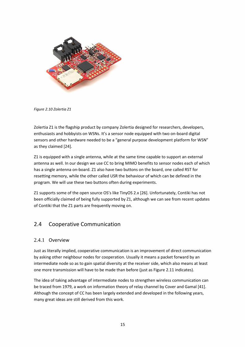
For our implementation, we use Zolertia Z1 (Figure 2.10) as our physical development platform.

MAC Layer

Announcement Layer Rime primitives and protocols

Figure 2.9 architecture of announcement layer

15

Figure 2.10 Zolertia Z1

Zolertia Z1 is the flagship product by company Zolertia designed for researchers, developers,

enthusiasts and hobbyists on WSNs. It’s a sensor node equipped with two on-board digital

sensors and other hardware needed to be a “general purpose development platform for WSN”

as they claimed [24].

Z1 is equipped with a single antenna, while at the same time capable to support an external

antenna as well. In our design we use CC to bring MIMO benefits to sensor nodes each of which

has a single antenna on-board. Z1 also have two buttons on the board, one called RST for

resetting memory, while the other called USR the behaviour of which can be defined in the

program. We will use these two buttons often during experiments.

Z1 supports some of the open source OS’s like TinyOS 2.x [26]. Unfortunately, Contiki has not

been officially claimed of being fully supported by Z1, although we can see from recent updates

of Contiki that the Z1 parts are frequently moving on.

2.4 Cooperative Communication

2.4.1 Overview

Just as literally implied, cooperative communication is an improvement of direct communication

by asking other neighbour nodes for cooperation. Usually it means a packet forward by an

intermediate node so as to gain spatial diversity at the receiver side, which also means at least

one more transmission will have to be made than before (just as Figure 2.11 indicates).

The idea of taking advantage of intermediate nodes to strengthen wireless communication can

be traced from 1979, a work on information theory of relay channel by Cover and Gamal [41].

Although the concept of CC has been largely extended and developed in the following years,

many great ideas are still derived from this work.


16

Cooperative communication has been proved by many papers about the improvement of

packet-reception-rate (PRR), transmitting speed, interference reduction and other multiple

input multiple output (MIMO) benefits by taking advantage of intermediate nodes to gain

spatial diversity (Figure 2.11). This is extremely meaningful in low-power WSNs where each

node often contains only one single antenna.

Figure 2.11 explains the basic idea of CC. Node A can improve the low-quality communication

with Node B by taking advantage of Node C’s forwarding which has high-quality channels to

both Node A and Node B. Here the quality can be speed or reliability or both in different context.

For example in [14] and [15], a higher throughput and lower interference are both achieved by

using a protocol called CoopMAC, which is designed based on IEEE 802.11.

2.4.2 Strategies of cooperation

There are different strategies to reach cooperation depending on different contexts and which

layer the implementation lies.

In the PHY layer [42-44] usually cooperation means an additional copy at the receiver side

where two copies of signals will be combined to get a single packet with higher robustness

against signal fading. In this case only one packet will be received in the upper layers, and this

packet should be exactly the same with the original one sent from the original sender.

In the higher levels including MAC [14, 15, 45], Network, or even Application layer, cooperation

is often reached in a way of two separate packets received by the destination at different time.

The receiver doesn’t combine the signals at PHY layer but leave the right to upper layers. These

two packets stand for the same original packet but do not have to be exactly the same. One of

them may contain additional information but all necessary original information should be kept

Node A Node B

Node C

a) Without Cooperative Communication

Node A Node B

Node C

b) With Cooperative Communication

Low quality transmission

High quality transmission High quality transmission

Low quality transmission

Figure 2.11 spatial diversity of Cooperative Communication

17

for recognition. For example, in CoopMAC [14], some areas in the MAC header may be changed

during relaying, but to upper layers the packets still seem exactly the same. In this way it also

increases the reliability since the transmission can be anyway considered successful as long as

any copy of the packet is correctly received.

These strategies of cooperation are different implementations for different contexts. Usually

they don’t co-exist at the same time.

By what strategy is used, CC can often be classified into the following categories (here we just

list some of them) [46, 47]:

a. Amplify and forward (AF) [48]

This method was first proposed on [49]. Just as the name implies, the relay simply

amplify and forward the received signal, even together with noise.

b. Classic multihop

The classic multihop can also be treated as a special case of CC, where only one route is

selected. Based on some routing algorithm, the sender is possible to set up a better

communication by hopping through multiple intermediate nodes. The receiver will only

receive one copy of the intended packet but the advantage is that overhearing is not

needed here.

c. Compress and forward (CF) [41]

d. Decode and forward (DF) [49-51]

Different with amplify and forward, which simply forwards the received signals together

with noise, DF tries to decode the packet first and re-encode the packet again before

relaying. In this way the noise can be largely reduced therefore improve the chance of

packets being correctly received.

e. Multipath decode and forward (MDF)

A full discussion of cooperation strategies is much too large to cover in this thesis. More

introductions can be found in the referenced papers above if readers are interested.

2.4.3 The overhearing

The overhearing feature is part of the preconditions for the concept of CC proposed in the very

beginning [41]. Relay offers help to the decoding at receiver side by overhearing transmissions

from sender and forward it when necessary.

Although the CC theory has been developed very much in the following years, in whatever way

CC is implemented, most of them still rely on the broadcast nature of wireless signals and make

nodes overhearing all packets even not sent to them. The overhearing is sometimes used to


18

realize opportunistic cooperation, or in other cases only used to extract neighbour information

like the channel qualities, for example, the CoopMAC protocol[14].

2.4.4 Relay selection

The intermediate doing forward is often called relay. It can be selected by sender or receiver

before transmission [14] or the relay itself can decide whether to forward an overheard packet

opportunistically, which is often called opportunistic relaying.

a. Direct transmission

A regular transmission can be one or more hops. The former one can be unicast or broadcast,

while the latter can be multihop. All of them set the address of next hop in packet header

without considering the performance of connections.

To be specific, in direct transmission a packet normally will go through all the network layers

when sending out, go up to some certain layer when forwarding (depends on which layer is

responsible of forwarding) and then go down again, and while receiving go through all the

network layers again but with an opposite way of sending. Take Contiki as an example, the data

flow of a direct transmission is like what Figure 2.12 says.

b. Opportunistic relaying

Opportunistic relaying only happens on relay side. The sender usually is not aware whether its

packets will be forwarded or not. When an intermediate node overheard a packet, it uses its

neighbour information to decide whether to forward it or not. If the answer is yes, then the

receiver of the original packet may receive two or even more the same packets if all the

channels work well.

Application layer

Rime layer

MAC layer

Physical layer

Application layer

Rime layer

MAC layer

Physical layer

Sender Relay Receiver

Application layer

Rime layer

MAC layer

Physical layer

Figure 2.12 data flow of direct transmission

19

The neighbour information can be got from different ways, either by extra exchanging packets,

or by analysing the information from normal packets.

If the intermediate node decides to forward a packet, it can also be two ways to do that. One is

to forward the exactly the same packet as it received. The other is only keep the data part and

other necessary parts intact and may edit a small part of headers before sending out. The

former way is more often to be seen in physical layer or MAC layer, while the latter way can be

higher to Rime layer.

c. Pre-Selected relaying

Relay can be pre-selected by sender or receiver. The decision can be sent to relay by extra

packets like 802.11’s RTS/CTS packets, or by annotating data packets. In the latter way the

sender should mark the address of relay in some area of packet header before sending out the

real packets. Then the relay can know whether it is selected and therefore do the forwarding as

requested.

The decision is again based on the channel information with neighbours. It can also be gained

from either specific extra packets or extracting from data packets or the combination of both.

2.5 Network Coding

2.5.1 Overview

The basic concept of NC is more like a mathematic way. Just as Figure 2.13 illustrated, multiply

packets can be coded into one packet so as to save the transmission times.

Node C

Node A

Node B

Packet 1

Packet 2

a) Without NC, two individual transmissions are needed

Node C

Node A

Node B

Packet 1 & 2

b) With NC, two packets are sent in one transmission

Figure 2.13 the concept of Network Coding


20

The idea of NC derives from a pioneering work by Ahlswede R. et al [5], which showed the utility

of NC for multicast in wired networks in 2000. After that the application of NC has been widely

broadened, for example, has been extended to wireless networks [52-56] which in fact have a

more urgent needs to improve their unreliability and broadcast nature.

The first implementation on wireless networks is presented in 2005 by Katti S. et al [18], named

COPE. It uses an opportunistic approach to network coding, which requires each node

overhearing all the time to learn neighbours’ status.

2.5.2 Coding Algorithms

The algorithm of encoding and decoding should be simple and make it possible to decode when

one coded packet is received. Exclusive or (XOR) is a commonly used algorithm for most of the

cases. It can be proved by mathematic that if packet 1, packet 2, …, packet n are XOR-ed

together, any of these packets can be decoded by the same operation XOR if the rest 1n

packets are already known, which can be explained by the formula (1) and (2).

1 2 ... ...encoded i np p p p p (1)

1 2 1 1... ...i encoded i i np p p p p p p (2)

The restriction of XOR algorithm asks any node trying to decode one packet should have the

ability to know all the other n-1 packets, which also means the network models should have

some limitation for the using of NC. The model in Figure 2.14 is a typical usage of NC. Node A

has a packet 1 sent to Node B, while Node B has another packet 2 sent to Node A. As an

intermediate node, Node C needs two individual timeslots to relay the two different packets.

After using NC, instead one timeslot is enough for transferring both packet 1 and packet 2 to

different nodes by taking advantage of the physical broadcast nature of wireless network. In this

model, both Node A and Node B have enough information to decode the received packet.

Node A Node

B

Node C Packet 1 to Node B Packet 2 to Node A

Packet 1 and 2 are encoded

Figure 2.14 a typical usage of network coding

21

Chapter 3. Design Considerations and Related Works

Although there are many research about CC, NC and NC-CC based on 802.11, it’s still new (on

implementation it’s still a blank page) for 802.15.4 and of course new for Contiki.

In this chapter we will discuss the issues we need to solve before we can carry out a feasible

plan.

3.1 Preconditions

3.1.1 The network environment

The model we use for evaluating our testbed is illustrated by Figure 1.2. But when doing design,

the testbed should be intended for more general network models.

Our target environment is 802.15.4-based WSN, which could be too obscure in design the

context. Here we list some important realities and assumptions to make the requirements of

testbed more specific:

a. No multicast. Since 802.15.4 doesn’t support multicast innately, many multicast-based

NC protocols would lose roots in such environment.

b. Ad hoc. Although the model in Figure 1.2 seems a fixed route during transmitting, as a

testbed, it should be able to adapt a changing environment quickly. Except the SINK

node, which functions different with any other nodes, in a general WSN each node can

be a sender or relay without prior notice. The senders may just start sending packets

when asked by some certain programs, and the relays can be dynamically chosen just

before transmission. What’s more, nodes can join or leave the network any time. All

these give our design a very high challenge.

c. RDC against overhearing. Since we use Contiki as nodes’ operating system, RDC will be

an indispensible function in the network. It makes nodes sleep as much as possible to

save energy. Therefore it will not be realizable to make assumptions like node is able to

overhear every packet in the air.

3.1.2 Other requirements

Besides all these network challenges the combination of which have never been worked out

before, our testbed should also satisfy other strict requirements:

Chapter 3: Design Considerations and Related Works

22

a. Backward compatible

So that nodes with our testbed enabled could also work well with those without;

b. Low coupling

So that people don’t have to change a lot when new version of Contiki released or

when network environment changed;

c. Easily configurable

With a little adjustment it can be adapted into different kinds of network models.

d. Power efficient

So the calculation should not be too complexity.

e. Memory limitation

Even one KB should be treasured on such sensor node.

f. Extensibility

Although the model we are using here has been reduced much complexity, the design

should be as extensible as possible. Model can be changed easily but an architect

design is hard to modify once implemented.

With all these constraints kept in mind, also based on the real structure of Contiki’s code, in the

following sections we give the analysis of how each part could be solved in the design of our

testbed.

3.2 Cooperative Communication

3.2.1 Positioning

The decision of where CC should function in the whole network stack may be the first barrier to

settle down before any other things could happen. However, this simple question relates to

many other factors and is also one of the most important decisions a designer should make.

As we talked in the previous chapter, the possible location of CC implementation could be

almost all layers: physical layer [42-44], MAC layer [14, 45, 57, 58], network layer (which is Rime

layer in Contiki), or even application layer. The way of implementing could also be different.

Some modified the existing protocol to extend the feature, some create an extra module

besides the existing ones to reduce the modification, others may choose to insert a totally new

layer (which can also be treated as a big module) between the existing layers to minimise the

impact to the original code.

23

Considering the principle we talked in the previous section that we shall keep the original

source code intact as much as possible, and the network structure of Contiki we introduced in

2.2, creating a new Rime primitive could be a best solution after balancing all the aspects.

3.2.2 Pseudo overhearing

Almost all current CC solutions rely on overhearing. Take network model in Figure 1.2 as an

example, regardless of whatever kind of relay strategies will be applied, relay has to overhear all

packets all the time in order to assist the transmission from sender to SINK.

However, in our low-rate WSNs, this precondition that relay should overhear all the time is not

realisable any more. In order to save the energy, Contiki uses RDC to control the node sleep or

wake up. When in sleep mode, the node is not able to overhear any packet. On the other hand,

if disable RDC to enable overhearing all the time, the energy consumption would be too high for

the whole network in which case the meaning of designing such testbed would be ridiculous.

One possible solution is to make SINK overhearing all the packets instead of relays. In our

assumption SINK is provided with continuous power supply therefore has no energy concerns.

Then the packet could be set relay to be its receiver but hide the real receiver in somewhere

else. In theory it should work but also requires a pre-selected relay before transmission.

3.2.3 Target packets

In a wireless network, many types of packets could co-exist peacefully, like broadcast, unicast or

multihop packets, each of which is used for different purpose but in an equivalent position

when transmitting in the air.

Packets in a typical WSN with Contiki installed can have the following types:

a. Strobe packets which are used to wake up sleepy nodes

b. Strobe-ACK packets which are acknowledgements for strobe packets

c. Data packets which can still be further categorized by different communication primitives

they are using, like unicast, broadcast, multihop, and etc.

d. Announcement packets, which is a mechanism provided by Contiki, used to exchange

neighbour information.

The packets CC would face depend on which layer CC locates.

If CC is implemented above MAC layer, then strobe-related packets will not be a concern since

they are only used in the MAC layer.

If CC is implemented in or above Rime layer, then announcement packets will be out of CC’s

control.


24

As we discussed in the previous sections, a realization as a Rime primitive could be a possible

solution in our context. But even in such implementation, CC can be designed to handle all Rime

packets or be separate with any other primitives, which is to say, when a CC communication is

set up, CC packets will work separately with other packets generated by for example unicast or

multihop. In the latter way, the decision gives back to application layer to decide whether to use

CC primitive or other existing primitives. Programs could control which data to send in

cooperated mode and which data be sent by simply unicast way. In the former way, a rewrite of

existing primitive is inescapable.

Considering all these factors we talked above, we suggest a new primitive should be the best

solution for CC in our context. In that case CC only needs to relay its own CC packets, which not

only simplifies the implementation, but also reduces unnecessary increase of transmitting

packets.

3.2.4 Relay determination

This section talks about who should be responsible to decide which relays to use during a

transmission. Many works have been done on this topic and a full discussion would be too much

for a thesis to contain. Generally, it can be decided by the sender [14, 15, 59], the receiver[60,

61], or the relay itself. The last case is also called opportunistic relaying.

Because of the reason we talked in 3.3.4, in order to realize pseudo overhearing, the sender has

to know which relay to use before sending out the packet. So in our situation, the sender would

be the best decision maker.

A relaying can also be two hops or more. As an initial design of testbed, we think two hops will

be tolerant in the beginning, since more hops is only a kind of tuning of two-hop relaying by

treating the relay as a sender and find a next relay again. Considering three hops or more at first

will largely increase the unnecessary complexity of design.

Relay can also be decided as one at a time or multiple nodes relaying the same packet together.

If regardless of network interference and the coming overhead, multiple copies of the same

packet could possibly increase the chance of receiving a correct packet. But in low-rate WSNs,

the increasing of packets could bring more even more drawbacks than the benefits it brings.

3.2.5 Relay strategy

Generally to say, there are two kinds of relay strategies to choose: either modify the packet or

keep it intact before forwarding.

The direct forwarding without modifying sounds much better at first sight, since it keeps the

packet integrity. But that would require CC implemented at physical layer, otherwise the MAC

layer would at least change the sender address in its header to be its own. Besides, it will have

difficulties to notify relay when to forward if the relay is decided by either sender or receiver.

Extra packets will be needed like CoopMAC does [14], while 802.15.4 doesn’t have 802.11’s

25

RTS/CTS mechanism. Moreover, since we use pseudo overhearing as we talked in 3.2.2, the

sender has to set relay as its receiver in packet’s MAC header, therefore anyway the relay has to

change this field before forwarding it to next hop.

3.3 Network Coding

3.3.1 Positioning

Just as the same situation CC faces, NC can also be put on almost all existing layers, or on a

totally new layer. It also depends on how the whole architect will be designed, for example, in

order to cooperate with CC, NC should possibly be placed somewhere below CC. The placement

will also certainly affect a lot on how the other modules will be designed.

Paper [18] and [19] presented a new coding architecture called COPE, which is designed for

802.11 based wireless networks. What it’s trying to solve has some similarities with ours, like

no-multicast, unpredictable traffic and dynamic environments. They put a new coding layer

between IP (which is Rime layer in our context) and MAC layers. Although their environment

also has many other differences with ours, we believe a new layer between Rime and MAC

should also work in our context.

3.3.2 Overhearing

Similar with CC, most of the NC implementations are based on relay’s overhearing all packets in

the air. The coding algorithm as we talked in 2.5.2 mathematically requires all encoded packets

should be able to be overheard in order to decode successfully at receiver’s side. However, in

our low-rate WSNs, RDC prevents relay to overhear all the time, thus the traditional way doesn’t

work anymore.

3.3.3 Coding targets

In many NC solutions they do coding for all kinds of packets, like unicast or multihop packets. In

out discussion, NC locates between MAC and Rime so it naturally also has the capability to code

all kinds of packets coming from upper layer.

However, in low-rate WSNs, the targeting packets should be carefully selected not to waste

unnecessary encoding which meant to fail for decoding. In many other implementations, the

success rate of decoding is sustained based on two preconditions: overhearing and learning

neighbour state. That means each relay should keep overhearing all the time which as we talked

before is not realisable in low-rate WSNs. Without overhearing, there will be only one copy for

each kind of packets except CC packets, and it will be not possible for receivers to decode but

only waste network bandwidth by re-transmitting all the time.


26

To conclude, in our case, we only consider coding and decoding those packets produced by CC.

To be more specific, those should all be outgoing packets.

3.3.4 Pseudo multicast

Although our model used in experiments (Figure 1.2) has just one mutual receiver, the design of

NC should be able to handle more complicated models for flexibility. Like in a typical butterfly

model (Figure 1.1), NC should be able to encode packets with different receivers. In that case,

since 802.15.4 doesn’t support multicast innately, the receiver address in MAC header should

be set as broadcast in order to mimic multicast. And it will be NC’s responsibility to check

whether it’s one of the intended recipients of the incoming ‘broadcast’ packets. To avoid

decoding all the packets each time blindly, NC may need to add some extra information in its

header.

3.3.5 Packets selection

To reach a high success rate for decoding, NC should be careful on packet selection when

encoding packets. A good decision would ask relay to gain enough information about what

packets its neighbours have received. For example, COPE [19] also gives out some assumption

that the node should have the knowledge of what its neighbours have heard in order to perform

its opportunistic coding.

This can be solved by sending exchanging packets each time a node receives a data packet. Then

it becomes a typical problem of exchanging neighbour information in a network, which already

has very good solutions on main networks like 802.11 or 802.3. However, in low-rate WSNs it’s

not realizable to afford such a huge network overhead. COPE [19] introduces an improved way

to annotate the data packet so the transmitting cost would be largely reduced. But it costs

much more calculation on each node, which will again aggravate the power consumption. By

any way it’s not possible for relay to know the real-time status of each neighbour. Relay has to

anyway guess based on limited information it gains.

Another solution is to carry out a good success/fail response mechanism. In the meanwhile, try

to make some algorithms to avoid failure as much as possible; either simple filters or dynamic

learning could work. The range of this topic is far beyond the purpose of this thesis.

3.3.6 Response mechanism

Failure can anyway happen. A proper response mechanism is necessary to assist the correctness

of the whole process.

A simple and common solution is to send ACK packets. One ACK for each success and each

failure is obvious too big overhead. Since there will possibly be more successes and less failure,

one may easily think that the ACK should only report when decoding fails. However, due to the

broadcast nature of wireless network, the decoding could be much easier than thought to fail if

27

relay has many neighbours around. The ACKs sent by every neighbour would again bring

network congestion.

Now let’s say we only send ACK when decoding is successful, still we have to decide whether

ACK should be sent on each successful step of decoding or only sent after the whole decoding

ends successfully. The answer is obvious in other regular NC applications. Due to the nature of

XOR algorithm, the packet with n packets encoded can be decoded completely only if the

receiver has already had all the 1n packets in the buffer. And in that case, only the last packet

decoded is the useful one since all other packets decoded will be duplicated. However, in NC-CC,

when NC works with CC, all packets are intended to be duplicated if no loss happens during

transmission. Duplication isn’t meaningless any more in this context. Any packet in the real

environment could drop by any reason, especially when two nodes have very bad signal

strength in low-rate WSNs, which is where CC helps. By combining NC with CC, the transmission

increased by CC could be largely reduced while still keep the possibility to recover lost packets.

If we send ACK on each step of decoding, it will certainly cause more ACK packets but on the

other hand may increase the chance of ACKs being received, which can further help improve the

buffer management on the relay side. As we will discuss later, NC layer needs to buffer some

outgoing packets for encoding. The buffer resource is very limited on some sensor nodes so it is

quite important for relay to cut these packets off the buffer when it’s already been received or

decoded by the correct node (in our context it’s SINK). An ACK mechanism for each individual

packet decoded out can help make the buffer efficient even the encoded packet cannot be

decoded completely or even some of the ACKs are lost while transmitting.

If no ACK is received after a certain time T, relay will re-send these packets individually without

being encoded, since the miss of ACK may be probably caused by an unsuccessful decoding so

that a simple re-transmission may not work again.

And if at the receiver side if a decoding does fail, we simply drop this packet and give no

feedback.

Another trouble is that since multiple packets will be decoded out if everything goes

successfully, it is important to specify when to pass the decoded packets to upper layer. Contiki

uses an event-driven kernel [25]. Therefore once NC gives out the control, the packet buffer will

possibly be polluted by other layers before it gets the control back. It’s NC’s responsibility to

protect packets before it completes all its process.

3.3.7 Buffer management

For encoding, only those CC packets are about to send out should be considered as encoding

candidates and buffered. The packet should be kept in the buffer until a certain time without

being encoded. Such packets should then be sent out directly.

When packets are selected for encoding, they should still be kept for a certain time T until ACK

received. If no corresponding ACK receives after T time, they should also be sent out directly

without being encoded.


28

For decoding, all the overheard CC packets should be buffered to maximum the chance of

successfully decoding. In our environment since only SINK is intended to decode, so that a

continuous overhearing is possible. When buffer is full, the oldest packet will be overwritten.

As we can see, packets for encoding and decoding are quite different and therefore should be

kept as two different buffers.

Since the memory is very limited on sensor nodes, all the two buffer will not be too large. Thus

no complicated searching algorithm is supposed to be applied here.

29

Chapter 4. Design and implementation

4.1 Overview

In order to implement NC-CC test-bed in Contiki, as we talked in the previous chapter, there

could be many possible ways of implementing. We brought out our solution in the target of

making the whole test-bed workable, additionally with possible performance enhancement. It

could not be the perfect one, but the meaning of our project is to encourage other researchers

by giving out an initial workable framework. In this chapter we’ll talk about how we design our

test-bed in detail, with brief explanation of why it should be like that.

After analysing the network stack of Contiki, we decide to create a new module to control the

logic of packet transmission for CC and add an entire layer to do the encoding/decoding things.

The network stack with NC-CC test-bed implemented is explained in Figure 4.1.

Figure 4.1 the network stack with NC-CC implemented

Just as Figure 4.1 illustrates, besides a test program in the application layer which we will

introduce in Chapter 5, we have a new communication primitive in Rime layer to do the work of

CC, and a new layer called NC layer inserted between Rime and MAC layer to take responsibility

of opportunistic coding.

a. The CC communication primitive in Rime layer

We add a new communication primitive for CC, on top of ‘broadcast’ primitive. It is

responsible of deciding which neighbour to relay, store suitable information in packet

header and exchange necessary information with neighbours.

b. The NC layer between Rime and MAC

Application Layer

Rime Layer

MAC Layer

Physical Layer

NC Layer

NC-CC Test Program

CC Protocol

Encoding / Decoding

RDC mechanism, CX-MAC

CC2420, overhearing

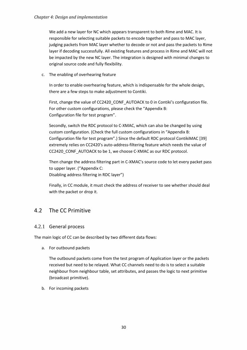
Chapter 4: Design and implementation

30

We add a new layer for NC which appears transparent to both Rime and MAC. It is

responsible for selecting suitable packets to encode together and pass to MAC layer,

judging packets from MAC layer whether to decode or not and pass the packets to Rime

layer if decoding successfully. All existing features and process in Rime and MAC will not

be impacted by the new NC layer. The integration is designed with minimal changes to

original source code and fully flexibility.

c. The enabling of overhearing feature

In order to enable overhearing feature, which is indispensable for the whole design,

there are a few steps to make adjustment to Contiki.

First, change the value of CC2420_CONF_AUTOACK to 0 in Contiki’s configuration file.

For other custom configurations, please check the “Appendix B:

Configuration file for test program”.

Secondly, switch the RDC protocol to C-XMAC, which can also be changed by using

custom configuration. (Check the full custom configurations in “Appendix B:

Configuration file for test program”.) Since the default RDC protocol ContikiMAC [39]

extremely relies on CC2420’s auto-address-filtering feature which needs the value of

CC2420_CONF_AUTOACK to be 1, we choose C-XMAC as our RDC protocol.

Then change the address filtering part in C-XMAC’s source code to let every packet pass

to upper layer. (“Appendix C:

Disabling address filtering in RDC layer”)

Finally, in CC module, it must check the address of receiver to see whether should deal

with the packet or drop it.

4.2 The CC Primitive

4.2.1 General process

The main logic of CC can be described by two different data flows:

a. For outbound packets

The outbound packets come from the test program of Application layer or the packets

received but need to be relayed. What CC channels need to do is to select a suitable

neighbour from neighbour table, set attributes, and passes the logic to next primitive

(broadcast primitive).

b. For incoming packets

31

Invoked by lower channel (broadcast channel), decide what to do (drop; pass to

application layer; relay) by checking attributes. If the packets need to be relayed to

other nodes, the logic is again the same with outbound packets.

4.2.2 Announcements

In order to exchange RSSI information, each node periodically broadcast announcement packets

to its neighbours.

In current implementation, two kinds of RSSI values are needed for relay selection. R-RSSI can

be extracted from any kind of packets received. So actually announcements are mainly used to

transfer D-RSSI only. The overhead may seem too large from some aspect. But in Contiki,

announcements can be shared by many communications together, which means many values

for different purposes will be put in one announcement packet, in which case the average

overhead would be largely reduced.

When one announcement is received, CC updates both R-RSSI and D-RSSI information in

neighbour table. New entry will be created if no existing neighbour found in the table. If the

announcement is from the SINK, then the R-RSSI extracted will be the newest D-RSSI of its own,

which will be put in the value part of next outbound announcement.

The announcement mechanism is provided by Contiki and is still being improved. Currently it

doesn’t leave much interface for customization. But by using a custom configuration file

(Appendix B), it’s still possible to make some adjustment. In our experiments, we changed the

sending frequency as you can see in Appendix B.

4.2.3 Neighbour table

CC maintains a table to keep track of all reachable neighbours. But only those neighbours that

can also reach SINK will be kept. The data is regularly updated for relay selection. If no

announcements from a neighbour are received for a certain time T, the corresponding entry will

be removed from the table. Here we set T as 200 seconds.

The following data is stored for each neighbour (Table 4.1 gives an example of neighbour table):

a. R-RSSI. The RSSI value between the host and the neighbour (the potential relay).

b. D-RSSI. The RSSI value between the neighbour and the destination (in our model it is

always the SINK). The SINK’s D-RSSI is set to be an unreasonably high value.

Table 4.1 an example of neighbour table

Address R-RSSI D-RSSI

15.0 -67 -70

17.0 -77 -58

12.0 -79 127


32

In resource constraint environment, memory usage should also be carefully controlled. We set a

maximal value for the number of neighbours could be stored. In current implementation it is 8.

4.2.4 Relay selection

As we mentioned above, our relay selection is based on comparing two types of values in the

neighbour table, S RRSSI and R DRSSI . Every neighbour node in the table might be selected

as next relay, which can be either destination or other node.

In order to select an overall best channel, we search in the table to find the node with best

value of the worse one between S RRSSI and R DRSSI . We call it the best-worst algorithm.

Define R as the set of all nodes recorded in the neighbour table and iR as the i th node in R.

The algorithm can be formulated as (3):

I iiS R R DR R

Best Relay Max Min RSSI ,RSSI (3)

When a relay is selected, it’s marked as the receiver at MAC layer while CC stores address of the

final receiver (which we called E-receiver) in Rime header, as well as other attributes. Due to the

variation of link qualities, the selected relay can be either destination or other nodes. Thus the

transmitting hops can be one or more. To simplify the experiments and avoid transmitting loops,

here we force the maximum hops to be two.

4.2.5 Packet header

Since CC is located in Rime stack, the packet header is managed by Chameleon’s header

transformation module and all we should do is to define the attribute list we need.

To make it as short as possible, we only defined three attributes in CC:

a. The address of E-Sender

Since the sender address in MAC header will be changed while forwarding, we have to keep

the address of original sender.

b. The address of E-Receiver

The same reason of E-Sender, we keep the address of end-receiver in CC headers.

c. The packet id

Because we modified some header of the packet while forwarding, we need an ID to

identify the same packet. To save the space, we use only one byte to present this id and

identify an identical packet using the combination of this packet id and E-Sender together.

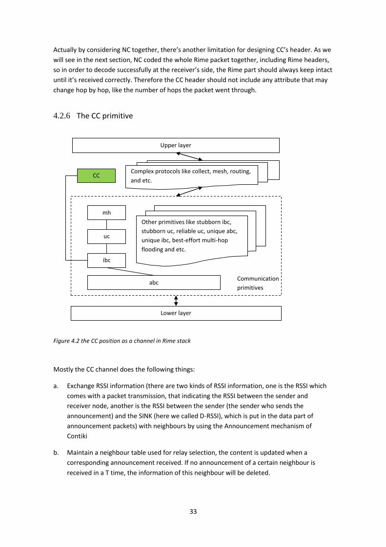
33

Actually by considering NC together, there’s another limitation for designing CC’s header. As we

will see in the next section, NC coded the whole Rime packet together, including Rime headers,

so in order to decode successfully at the receiver’s side, the Rime part should always keep intact

until it’s received correctly. Therefore the CC header should not include any attribute that may

change hop by hop, like the number of hops the packet went through.

4.2.6 The CC primitive

Figure 4.2 the CC position as a channel in Rime stack

Mostly the CC channel does the following things:

a. Exchange RSSI information (there are two kinds of RSSI information, one is the RSSI which

comes with a packet transmission, that indicating the RSSI between the sender and

receiver node, another is the RSSI between the sender (the sender who sends the

announcement) and the SINK (here we called D-RSSI), which is put in the data part of

announcement packets) with neighbours by using the Announcement mechanism of

Contiki

b. Maintain a neighbour table used for relay selection, the content is updated when a

corresponding announcement received. If no announcement of a certain neighbour is

received in a T time, the information of this neighbour will be deleted.

abc

Lower layer

ibc

uc

mh

Other primitives like stubborn ibc,

stubborn uc, reliable uc, unique abc,

unique ibc, best-effort multi-hop

flooding and etc.

Communication

primitives

Upper layer

Complex protocols like collect, mesh, routing,

and etc. CC


34

c. Decide which neighbour to be the next hop (relay selection), currently we support two

hops at most. The selection algorithm is based on the RSSI and DRSSI. If one neighbour has

the best worst-value of RSSI and DRSSI, it is selected as next relay.

d. Keep necessary information while relaying. An isolated packet ID is used for identification.

4.2.7 Configurable parameters

To let others easily adjust CC for different purposes, we use many macro definitions on

important variables.

a. The starting number of packet ID

b. Whether to enable text debug information (for neighbour-table the text debug

information can be separately controlled and have special function to print out the

neighbour-table in a human-readable form)

c. Whether to enable LED debug information

d. The maximal neighbours could be stored in the neighbour-table

e. After how long time without receiving announcements from a certain neighbour should

remove it from the neighbour-table

4.2.8 Overheads

Although CC may bring WSNs spatial diversity, reliability, and other MIMO benefits, it also

brings some extra burdens to the networks.

One is the introduction of announcement packets. Announcement is a mechanism provided by

Contiki, which is out of CC’s control on when and how to send the packets. In order to make a

good relay selection, CC actually asks for relatively frequent information exchanging with other

neighbours, which means there will be more announcement packets produced, the existence of

which will cause more packet conflicts and should not be ignored.

In our implementation, we put CC in Rime layer to take advantage of existing primitives. In such

design it requires overheard packets to go higher than putting CC in physical layer or MAC layer.

It will cause more time to handle each packet therefore the overall efficiency might be

influenced. However, we don’t how much it really will have.

In order to enabling overhearing, we turned off CC2420’s auto-address-filtering feature. This

feature can drop packets which are not for the node quickly without passing them to MAC layer.

The turning off will prevent nodes’ fast sleep which is important for power saving.

35

4.3 The Networking Coding Layer

4.3.1 Overview

The NC layer works like a transparent middleware between Rime and MAC layer. No extra

actions should be done for either Rime layer or MAC layer. Each other layer just works like

before and the NC layer will do all the encoding / decoding work without affecting the original

network stack.

Our NC layer employs opportunistic coding just like COPE [18] does. It selects multiple packets

to encode just before sending, or buffer them for a short certain time when there's no match

for encoding. After successfully decoding, all decoded packets are passed to Rime layer one by

one immediately.

4.3.2 Work flow

The main logic of NC layer can be described as following:

a. For outbound packets

Every outbound packet has to pass NC layer before getting to the MAC layer. The layer

is triggered by the upper Rime layer. Every packet should be checked first and only

those produced by CC channel would be treated specially. Other packets would be

simply given to MAC layer without any modification (just like transparent).

When a CC outbound packet is detected, the NC layer checks the outbound buffer to

see if there's any waiting packet meets the encoding requirement. There is an algorithm

specially to judge whether it should be encoded or not. Encode as many packets as

possible together until it reaches the MAX_ENCODED limit. If there is no matching

packet to encode, put the packet in outbound buffer, and send it directly if it is not

encoded in a certain time T1.

When n packets are encoded, they are still kept in the buffer until the corresponding

ACKs arrive, or send individually after a T2 time.

b. For incoming packets

Similar with outbound process, every incoming packet have to be checked by NC layer

before getting to Rime. Only the packets with NC header will be specially treated (let's

call them NC packets), while others be directly passed to upper layer.

The NC header has different kinds of structures, indicating whether it is an encoded

packet and how many packets encoded if so, or an ACK packet which means a

successful decoding finished. The detail will be talked later.

If an encoded packet detected, the NC layer will check the incoming buffer to see if

there's any packet able to help decoding. Every decoded packet is stored in the


36

incoming buffer for possible future decoding and also passes to the upper layer Rime.

An ACK is generated to say how many packets are successfully decoded.

4.3.3 Buffers

In order to support encoding and decoding, the NC layer maintains two different buffers, one

we called outbound buffer, which stores packets waiting to be encoded, another we called

incoming buffer, which is a packet library used for decoding.

a. The outbound buffer

NC only buffers CC’s packets in the outbound buffer. When it’s about to forward a

packet from CC, first it checks whether there are packets already in the buffer that can

be encoded together. If there are, then NC encodes them and sends the coded packet

out. The original packets will still be kept in the buffer for a certain time until an ACK

received.

If there’s no match currently, NC buffers the packet and waits a short time to see if

another packet needs to be sent out. After a certain time without being encoded, the

packet will be sent out directly and removed from the buffer immediately.

If a packet has been encoded and sent for a certain time without receiving any ACKs, it

will also be sent out again but without being encoded and also removed from the buffer

immediately.

b. The incoming buffer

The incoming buffer is used for decoding which is only at the SINK side in our context.

SINK has two sources of receiving packets, one from relay, and the other from senders.

Packets from senders are not encoded but still will be put in the incoming buffer for

decoding in the latter time. A general principle is that all CC packets will be buffered in

the incoming buffer, since we don’t know what kind of coded packets will be received

that require a pre-received packet for decoding.

The size of incoming buffer theoretically should be as large as possible. By the memory

limitation in our context, we set the maximal size as only 10 packets. The oldest one will

be overwritten by a new packet when buffer is full.

To identify a packet, we use the combination of the packet id and the address of E-

sender.

4.3.4 Packet header

In order not to bring chaos to Rime layer and MAC layer, the NC layer has its own header (as

Figure 4.3 illustrates). The NC header is not controlled by Chameleon’s header transformation

module.

37

a. For outbound packets, it adds the header before passing to MAC layer, without

modifying the Rime header. Since the MAC layer doesn't care about how the higher

layers deal with packets header, the NC header seems transparent both to Rime and

MAC layer.

b. For incoming packets, the MAC layer will remove its own MAC header before passing

the control to NC layer. Then the NC layer analyses the NC header and removes it

before passing above. Again, the NC layer becomes transparent both to upper and

lower layers.

Figure 4.3 the place of NC header

According to the type of packets, we define four different NC headers (Figure 4.4):

a. Single packet without encoded

The reason why we have to add an extra header in front of a not-encoded packet is that

when a new packet arrives, passed by MAC layer, on NC layer it has no idea of how to

get the ESENDER and E-PID information, therefore not possible to buffer it for the usage

of decoding next time.

b. Multiple encoded packets with the same destination

Right now our implementation in the code is the same with multiple destinations,

should be changed to how it is designed.

c. Multiple encoded packets with multiple destinations

It is the structure used to support pseudo multicast which we talked in 3.3. By having

such information in the header, NC doesn’t have to decoding tentatively without

knowing the exact receivers.

d. ACK packets


38

4.3.5 Packet length

If multiple packets with different length are encoded, the final length is the same with the

longest packet before encoding (Figure 4.5). And accordingly, when decoding, it will only be

possible to decode out packets all with the same length. It can be easily solved by adding a

length in the header. But in this stage it may not be a big problem thus we would rather leave it

to further improvement.

Channel NO.

Single packet without encoded

Type E-Sender PID

Channel NO. Type Receiver Num E-Sender PID

Multiple encoded packets with the same destination

… …

n the same structures n

Channel NO. Type E-Sender Num Receiver PID

Multiple encoded packets with multiple destinations

… …


Channel NO. Type E-Sender Num PID

ACK packets


Figure 4.4 four kinds of NC headers for different packets

39

Figure 4.5 the length of packet encoded

4.3.6 Encoding

We use XOR algorithm to encode and decode multiple packets. The idea of XOR has been

mentioned above as formula (1) and(2).

Since NC locates below the Rime, it is reasonable that all payloads to NC layer, including Rime

header and application data is encoded. But in this way we lose the information of what packets

are encoded. To solve this problem, as we can see from 4.3.4, some necessary information of all

encoded packets is stored in NC header, like the packet id, E-Sender and receiver.

We set a MAX_ENCODED parameter to say how many packets can be encoded together at most.

But the actual number depends on how many matching packets found in the outbound buffer.

The selection of encodable packets is done with a basic algorithm as following, which however

can be easily extended in the future.

a. We use two attributes to identify one packet: packet ID and E-sender. Packet ID is the id

generated by CC and set as an attribute for cross-layer use. To make it clear, it is

separated from the packet ID in MAC layer.

b. Packets with the same E-sender should not be encoded together. The reason is based

on the trait of wireless transmission and XOR algorithm. The XOR algorithm needs the

other 1n packets available if n packets are encoded. And in a wireless scenario, if the

signal channel is physically bad between two nodes, the packets from the same e-

sender are in a higher possibility to drop, which means, the less successful rate to

decode the packets.

4.3.7 Decoding

The decoding is the inverse operation of encoding. If n packets are encoded in a NC packet, you

need 1n of them right available in the incoming buffer in order to decode successfully.


40

By analysing information of encoded packets from NC headers, NC layer then check the

incoming buffer to see if it has all the packets needed.

a. If there are not enough decoding packets, the decoding is failed and no further action

will be performed.

b. If all the packets are decoded successfully, all of them are passed to upper layer Rime,

one by one. An ACK packet is sent with all decoded packets' information.

One thing is remarkable that the decoded packets should be passed to the upper layer only

when all packets are decoded successfully. That means all the decoded packets should be saved

with entire information before the decoding end. Otherwise the packet buffer where all the

decoding happens will be polluted by upper layers once NC passes packets to Rime.

The optimization of NC layer is talked in Chapter 6 “Conclusion & Future work”.


With easily modification (usually just change a value of the corresponding variable), NC allows

adjusting its behaviour when needed:

a. Whether to print out text debug information

b. Whether to print out report information (which concise format for statistics)

c. The channel number of NC

d. Whether to enable NC

e. The timeout period for waiting for ACKs

f. The maximal number of packets could be encoded together at one time

g. The maximal number of packets stored in outbound buffer

h. The maximal number of packets stored in incoming buffer

i. The timeout period for storing outbound packets, after this period if the packet hasn’t

been encoded and sent out, it will be sent out directly without encoded

4.3.9 Overheads

The NC theoretically should not have many overheads since it’s just a kind of decorating work to

the existing packets. However, to make the whole mechanism work, some prerequisites need to

be settled which can turn to be overheads.

41

The biggest of them is the buffer management. Either encoding or decoding needs to buffer a

number of packets, which will almost fulfil the small memory of sensor nodes. And it takes time

to copy large block of memories from here to there.

The second heaviest cost could be the processing of headers. The NC header not only adds

overhead to each packet transmission, but also cost some time to pack and unpack it each time.

Because of the position NC locates, it will not have the benefits of Chameleon which has a

header transformation module. Each bit should be handled by NC itself. The definition of

several different kinds of headers makes the work even more complicated.

Moreover, sometimes the relay has to resend the packets if no ACK packets are received in a

certain time, which means they are probably not decoded successfully.

Finally, the introduction of ACK packets could also increase the network congestion.

Chapter 5: Experiments and Evaluation

42

Chapter 5. Experiments and Evaluation

5.1 The Test Program

To evaluate the performance of CC&NC, we need to set up different network models. The test

program we design supports customized scenario (network models) by easily configuration and

a list of useful features like set up the scenario, dispatch different task to different nodes,

control the power, print detail information for debugging packets transmission or concise

information for statistics.

5.1.1 Feature list

a. Distribute different task to different nodes with the same program. That means, you

don't have to write different programs and upload them to different nodes. All

functions are written in one program. What you have to do is set up the roles for

different nodes, upload the same program to all nodes, and then each node will

perform by its role you predefined.

b. Multiple ways of printing information. There are three kinds of formatted information

can be chosen to print out, short and tidy report for statistics, important debugging

information, or even more detail binary information for some specific debugging. You

can switch on one or all of them, depending on the situation.

c. LED indicator. It's not always convenient to rely on the printed information especially

when doing experiment with more nodes than the laptops. We make it possible to

know some simple state information by taking the advantage of different LEDs.

Receive a packet: flush the BLUE light once. Either the SINK or the relay will have this

indicator.

When the USR button is pressed: the GREEN light will be on for a few seconds (can be

configured) and turns to off when start the real process.

When a packet is forwarded on relay side: relay will toggle the GREEN light once.

When all packets are sent: the sender will keep the GREEN light on.

d. Multiple ways to trigger some specific features. Usually the programs start working

when the nodes are reset, for example, when the firmware is uploaded, which is not the

experimenters want. We want the node to send packets in some certain time, for

example, when all other nodes are ready and reset. This test program offers two ways,

time and button, to control when a certain feature should start working. By clicking the

43

USR button, nodes will start working depends on their predefined roles, with a PRELUDE

time delayed:

SINK: start to collect and print the noise signal strength in a pre-defined frequency.

RELAY: start to collect and print the noise signal strength in a pre-defined frequency.

SENDER: start to send packets in a static or dynamic configurable interval.

e. Automatically change the transmission power in runtime. The starting power and the

changing order can be easily predefined.

f. Make the packet length fixed, which is very helpful for some statistics.

g. Support multiple senders and statistic count of received packets by each.


By easily changing the value of a configuration, one can make many adjustments to our test

program. A full list can be found in the “Appendix D:

Configuration dictionary of test program”.

a. Which node should be the SINK

b. The frequency of sending announcement packets

c. Whether enable the overhearing feature

d. Which RDC mechanism to use

e. Which powers should be tested

f. The amount of packets to send

g. The time interval of sending packets

h. Whether the sending should be random within the time interval

i. Maximal length of the data part

j. Maximal senders should support

k. The time of PRELUDE to wait before really start working

l. Whether to print out debug information

m. Whether to print out detail debug information like the binary data of packets

n. Whether enable the LEDs indicator

o. Whether to print out short brief report information


44

5.2 Overview of results

When evaluating only CC, we use PRR as the main measurement. The CC performs very well

when power is higher than -10 dBm, no significant difference compared with unicast (all around

100% PRR).

When comparing NC-CC with CC, we use both PRR and “Number of transmissions” as

measurement. When using a power higher than -7 dBm, the PRR becomes a little bit lower

under NC-CC than under only CC, e.g., 98.50% under NC-CC and 100% under only CC using 0

dBm, which means the introduce of NC may increase the chance of packet collisions but not

significantly (may depend on different network environments). In the meanwhile, the number

of transmissions is largely reduced by having NC enabled. The number of packets physically

received by antenna on the receiver side is 504 when using NC-CC and 1000 when using only CC.

The throughput is almost doubled.

However, all the performance mentioned above became dramatically unstable when the power

is set lower, for example, equal or less than -10 dBm. We may infer that in low powers due to

the introduction of announcement and extra node’s interference, it becomes easier for packet

collisions and nodes lost. A detail explanation may need further experiments.

For another analysis of these experiments, especially on low powers situations, please check the

thesis by my partner Yitian Yan [62].

5.3 Experiment 1: unicast & CC comparison

To test whether CC functions well, we designed three different models for evaluation (as listed

in Table 5.1):

a. no relay is used, to compare the performance with unicast communication primitive

b. one potential relay, to test how relay selection algorithm improves the overall

performance

c. one relay is forcedly used to forward each packet from source

45

Table 5.1 Experiment Parameters of Comparing CC’s performance with unicast’s

Parameter unicast CC(no relay) CC(one relay) CC(relay forced)

Number of senders 1 1 1 1

Number of relays 0 0 1 1 (forced)

Number of destinations 1 1 1 1

Distance between source and destination (m) ~10

Transmit power level (dBm) 0, –1, –3, –5, –7, –10, –15

Number of packets sent per sender per each power level

1000

Size of MAC frame (bytes) 20

We also compare the RSSI value at the SINK side. When using CC with no relay, we can see that

although the average value is quite close, the RSSI detected at the SINK side (Figure 5.2) is much

more unstable than unicast (Figure 5.1), which is possibly caused by extra announcement

packets. (In the figure power 0xFF means 0 dBm)

Figure 5.1 the RSSI value of unicast detected at the receiver side


46

Figure 5.2 the RSSI value of CC detected at the SINK side

When using force relayed CC, we filtered the RSSI values from those packets forwarded by relay

(see Figure 5.3), the average value turns to quite better than unicast or the same model from

the sender (see Figure 5.4), which on the other hand proves that the relay selection of CC does

improve the channel quality by choosing a relay with better connection with destination. But

due to the instability of signal strength in this model (mainly because of the existence of extra

node and extra packets), the sender doesn’t always choose the relay as next node, like the

experiment with one relay proves.

47

Figure 5.3 the RSSI value of packets from relay, detected at the SINK side

Figure 5.4 the RSSI value of packets from sender, detected at the SINK side


48

5.4 Experiment 2: CC & NC-CC comparison

While comparing CC with NC-CC, we use the network model in Figure 1.2. Table 5.2 lists the

parameters we use.

Table 5.2 Experiment Parameters of Comparing NC-CC's performance with CC’s

Parameter CC NC-CC

Number of senders 2 2

Number of relays 1 (forced) 1 (forced)

Number of destinations 1 1

Distance between source and destination (m)

~10

Transmit power level (dBm) 0, –1, –3, –5, –7, –10, –15

Number of packets sent per sender per each power level

500

Size of MAC frame (bytes) 20 25

We analysed data both from SINK and relay. By using the printed report information by our test

program, we can also know the status of encoding and decoding each time. Here we only count

the number of timeout after sending out encoded packets, which possibly means unsuccessful

decoding at receiver’s side.

First we get some results from experiments indoors which we list in Table 5.3 (data under low

power are filtered. Please refer my partner’s thesis [62] for more analysis).

Table 5.3 results of indoor experiment of comparing NC-CC with CC (power: 0dBm)

Measurement CC NC-CC

Packets sent by relay 1000 503

Received data packets from node 17.0 500 496


Packet reception ratio 99.9% 99.5%

Packets timeout - 16

We can see from the table that by enabling NC together with CC, the overall packets in the air

are largely reduced into almost half. The overhead is in contrast very little, with only 16 times

re-transmission in a 1000 traffic.

However, we should also be aware that in our experiments we use a fixed sending rate on both

senders, which is 0.8 second per packet. And we make the senders start sending almost at the

same time therefore the relay is possible to get a very high encoding rate. In the reality, since

49

we use opportunistic coding in our design, there may not have so large chance for relay to find

encodable packets each time.

Although in this experiment we can see that NC doesn’t introduce much packet loss to the

whole network, still we would like to see how the performance will be with the same settings

but outdoors.

The results in Table 5.4 came from our university’s one packing lot which has fewer fences

around. Again, we can see that NC-CC improves the throughput dramatically with just a few

costs, although the change of place doesn’t help in this case. The timeout may due to failed

decoding, the loss of encoded packets, or the loss of ACKs, which on the other hand also shows

the timeout mechanism works very well, more or less improve the stability of our architecture.

Table 5.4 results of outdoor experiment of comparing NC-CC with CC (power: 0dBm)

Measurement CC NC-CC

Packets sent by relay 1000 504



Packet reception ratio 100% 98.5%

Packets timeout - 17

Chapter 6: Conclusion & Future works

50

Chapter 6. Conclusion & Future works

6.1 Conclusion

This thesis aims at realizing a NC-CC testbed in 802.15.4-based WSNs and encourage other

researchers continue improving this initial framework.

From experiments we can see that our design and implementation function properly. With a

new CC communication primitive implemented in Rime layer and a new NC layer between Rime

and MAC, we have been able to select a proper next hop among neighbours which realizes

spatial diversity, and we are also able to encode/decode CC packets transparently to reduce

number of transmissions, which in turn increases the network throughput.

In this thesis, many innovative ideas are inspired which have never been carried out before. The

most recognizable two mechanisms are:

a. Pseudo overhearing (section 3.2.2).

b. Pseudo multicast (section 3.3.4).

And of course the testbed itself is also totally new in this area, including the positioning of NC-

CC (section 3.2.1 and 3.3.1), and many followed details.

We have to confess that some faultiness still exists in our framework, but there are more

remarkable ideas and works that should be a big step in this area. We hope our testbed can be

further developed in the future to be a more robust and more practical tool for more

researchers.

6.2 Future work and possible optimization

The current design still has many shortages which have to be addressed before putting it into

real practices:

a. The position of NC layer might be optimized.

We did think about putting NC layer a bit upper. It should still be not higher than Rime

but might take some advantage of the Chameleon architecture. One possible solution is

to put it under abc primitive but higher than the header transformation module. The

network stack will be like in Figure 6.1.

51

Figure 6.1 one optimization of the design of NC layer

The advantage of this design is it can fully integrate NC with CC. NC can combine the

attributes of CC and NC and pass them to the header transformation module, in which

case there will be only one NC-CC header instead of two separate ones. The existence

can still be transparent to other layers and NC doesn’t have to deal with packing and

unpacking of headers any more, which can simplify the whole process a lot.

b. Headers of both CC and NC need to be optimized.

They should be as short as possible and as we talked above we may combine them

together since anyway NC-CC needs both of them in order to function correctly.

c. Extend to more than two hops.

In the current design we only support maximal-two-hop relaying to avoid some

complicated problems like loop-relay. We think such simplification should be tolerant in

the first stage like CoopMAC [14] did. But it should be extended in the future to support

more freely scenarios.

d. Smarter announcement.

The announcement mechanism is provided by Contiki originally and we only modified

some parameters for adjustment. Since Contiki authors are still working on this part, it

can be smarter in the future so as the drawback of announcement can be largely

reduced.

e. Beacon might be enabled.

If the beacon mode defined in 802.15.4 can be implemented in Contiki, the network

coordinator can then control the wake up time of the attached devices. In that case

more energy can be saved. But it might have conflict with RDC layer.

f. Better algorithms.

Algorithms might all be improved, including relay selection of CC, encoding/decoding

mechanism of NC. Such open questions each can be an individual topic and also be

found in many other papers.

We hope that our trial implementation could lead to a good start of this direction and our

contribution here could help the advancement of NC-CC practicing.

52

Bibliography

[1] S. Misra, I. Woungang, and S. C. Misra, Guide to wireless sensor networks: Springer, 2009. [2] K. J. R. Liu, A. Sadek, W. Su, and A. Kwasinski, Cooperative communications and networking:

Cambridge Press, 2009. [3] J. N. Laneman, "Cooperative communications in mobile ad hoc networks," IEEE Signal

Processing Magazine, vol. 1053, 2006. [4] V. Stankovic, A. Host-Madsen, and Z. Xiong, "Cooperative diversity for wireless ad hoc

networks," IEEE Signal Processing Magazine, vol. 23, pp. 37-49, 2006. [5] R. Ahlswede, N. Cai, S. Y. R. Li, and R. W. Yeung, "Network information flow," Information

Theory, IEEE Transactions on, vol. 46, pp. 1204-1216, 2000. [6] S. Sharma, Y. Shi, J. Liu, Y. T. Hou, and S. Kompella, "Is network coding always good for

cooperative communications?," in INFOCOM, 2010 Proceedings IEEE, 2010, pp. 1-9. [7] S. Sharma, Y. Shi, J. Liu, Y. Hou, S. Kompella, and S. Midkiff, "Network Coding in Cooperative

Communications: Friend or Foe?," Mobile Computing, IEEE Transactions on, pp. 1-1, 2011. [8] T. E. Hunter, "Coded cooperation: a new framework for user cooperation in wireless

networks," University of Texas at Dallas, 2004. [9] J. Hu, P. Fan, K. Xiong, S. Yi, and M. Lei, "Cooperation-based Opportunistic Network Coding

in Wireless Butterfly Networks," in Global Telecommunications Conference (GLOBECOM 2011), 2011 IEEE, 2011, pp. 1-5.

[10] L. Xiao, T. Fuja, J. Kliewer, and D. Costello, "A network coding approach to cooperative diversity," Information Theory, IEEE Transactions on, vol. 53, pp. 3714-3722, 2007.

[11] K. Kandhway, "Network coding based cooperative communications," The University Of British Columbia, 2011.

[12] G. D. Menghwar and C. Mecklenbräuker, "Network coding for cooperative communications," in Proceedings of Junior Scientist Conference, 2008, pp. 105-106.

[13] M. Yu, J. Li, and R. S. Blum, "User cooperation through network coding," in Communications, 2007. ICC'07. IEEE International Conference on, 2007, pp. 4064-4069.

[14] P. Liu, Z. Tao, S. Narayanan, T. Korakis, and S. S. Panwar, "CoopMAC: A cooperative MAC for wireless LANs," Selected Areas in Communications, IEEE Journal on, vol. 25, pp. 340-354, 2007.

[15] T. Korakis, Z. Tao, Y. Slutskiy, and S. Panwar, "A cooperative MAC protocol for ad hoc wireless networks," in Pervasive Computing and Communications Workshops, 2007. PerCom Workshops' 07. Fifth Annual IEEE International Conference on, 2007, pp. 532-536.

[16] T. Korakis, Z. Tao, S. R. Singh, P. Liu, and S. S. Panwar, "Implementation of a cooperative MAC protocol: performance and challenges in a real environment," EURASIP J. Wirel. Commun. Netw., vol. 2009, pp. 1-19, 2009.

[17] T. Korakis, S. Narayanan, A. Bagri, and S. Panwar, "Implementing a cooperative MAC protocol for wireless LANs," in Communications, 2006. ICC'06. IEEE International Conference on, 2006, pp. 4805-4810.

[18] S. Katti, D. Katabi, W. Hu, H. Rahul, and M. Medard, "The importance of being opportunistic: Practical network coding for wireless environments," in Proc. 43rd Annual Allerton Conference on Communication, Control, and Computing, 2005.

[19] S. Katti, H. Rahul, W. Hu, D. Katabi, M. Médard, and J. Crowcroft, "XORs in the air: practical wireless network coding," in ACM SIGCOMM Computer Communication Review, 2006, pp. 243-254.

[20] H. Xu and B. Li, "XOR-assisted cooperative diversity in OFDMA wireless networks: optimization framework and approximation algorithms," in INFOCOM 2009, IEEE, 2009, pp. 2141-2149.

53

[21] S. Fu, K. Lu, Y. Qian, and M. Varanasi, "Cooperative network coding for wireless ad-hoc networks," in Global Telecommunications Conference, 2007. GLOBECOM'07. IEEE, 2007, pp. 812-816.

[22] C. Peng, Q. Zhang, M. Zhao, and Y. Yao, "On the performance analysis of network-coded cooperation in wireless networks," in INFOCOM 2007. 26th IEEE International Conference on Computer Communications. IEEE, 2007, pp. 1460-1468.

[23] D. Woldegebreal and H. Karl, "Network-coding-based cooperative transmission in wireless sensor networks: diversity-multiplexing tradeoff and coverage area extension," Wireless Sensor Networks, pp. 141-155, 2008.

[24] Zolertia. (2012, October 5). Z1 Platform. Available: http://www.zolertia.com/products/z1 [25] A. Dunkels, B. Gronvall, and T. Voigt, "Contiki-a lightweight and flexible operating system for

tiny networked sensors," in Local Computer Networks, 2004. 29th Annual IEEE International Conference on, 2004, pp. 455-462.

[26] (2012). TinyOS Home Page. Available: http://www.tinyos.net/ [27] L. M. S. Committee, "Part 15.4: Wireless Medium Access Control (MAC) and Physical Layer

(PHY) Specifications for Low-Rate Wireless Personal Area Networks (LR-WPANs)," IEEE Computer Society, 2003.

[28] A. Dunkels, F. Ö sterlind, and Z. He, "An adaptive communication architecture for wireless sensor networks," in Proceedings of the 5th international conference on Embedded networked sensor systems, 2007, pp. 335-349.

[29] A. Dunkels, "Rime-a lightweight layered communication stack for sensor networks," presented at the European Conference on Wireless Sensor Networks (EWSN), Delft, The Netherlands, 2007.

[30] SICS. (2012, October 5). Change MAC or Radio Duty Cycling Protocols. Available: http://www.sics.se/contiki/wiki/index.php/Change_MAC_or_Radio_Duty_Cycling_Protocols

[31] D. Estrin, R. Govindan, J. Heidemann, and S. Kumar, "Next century challenges: Scalable coordination in sensor networks," in Proceedings of the 5th annual ACM/IEEE international conference on Mobile computing and networking, 1999, pp. 263-270.

[32] R. Guerraoui and L. Rodrigues, Reliable Distributed Programming: Springer Verlag, Berlin, 2006.

[33] A. Dunkels, L. Mottola, N. Tsiftes, F. Ö sterlind, J. Eriksson, and N. Finne, "The announcement layer: Beacon coordination for the sensornet stack," Wireless Sensor Networks, pp. 211-226, 2011.

[34] P. Dutta and A. Dunkels, "Operating systems and network protocols for wireless sensor networks," Philosophical Transactions of the Royal Society A: Mathematical, Physical and Engineering Sciences, vol. 370, pp. 68-84, 2012.

[35] J. Polastre, J. Hill, and D. Culler, "Versatile low power media access for wireless sensor networks," in Proceedings of the 2nd international conference on Embedded networked sensor systems, 2004, pp. 95-107.

[36] W. Ye, J. Heidemann, and D. Estrin, "An energy-efficient MAC protocol for wireless sensor networks," in INFOCOM 2002. Twenty-First Annual Joint Conference of the IEEE Computer and Communications Societies. Proceedings. IEEE, 2002, pp. 1567-1576.

[37] M. Buettner, G. V. Yee, E. Anderson, and R. Han, "X-MAC: a short preamble MAC protocol for duty-cycled wireless sensor networks," in Proceedings of the 4th international conference on Embedded networked sensor systems, 2006, pp. 307-320.

[38] D. Moss and P. Levis, "Box-macs: Exploiting physical and link layer boundaries in low-power networking," Technical Report SING-08-00, Stanford University2008.

[39] A. Dunkels, "The ContikiMAC Radio Duty Cycling Protocol," Swedish Institute of Computer Science ISSN 1100-3154, 2011.

[40] A. Dunkels, O. Schmidt, T. Voigt, and M. Ali, "Protothreads: simplifying event-driven programming of memory-constrained embedded systems," in Proceedings of the 4th international conference on Embedded networked sensor systems, 2006, pp. 29-42.

[41] T. Cover and A. E. L. Gamal, "Capacity theorems for the relay channel," Information Theory, IEEE Transactions on, vol. 25, pp. 572-584, 1979.

http://www.zolertia.com/products/z1

http://www.tinyos.net/

http://www.sics.se/contiki/wiki/index.php/Change_MAC_or_Radio_Duty_Cycling_Protocols

54

[42] J. N. Laneman, D. N. C. Tse, and G. W. Wornell, "Cooperative diversity in wireless networks: Efficient protocols and outage behavior," Information Theory, IEEE Transactions on, vol. 50, pp. 3062-3080, 2004.

[43] G. Kramer, M. Gastpar, and P. Gupta, "Cooperative strategies and capacity theorems for relay networks," Information Theory, IEEE Transactions on, vol. 51, pp. 3037-3063, 2005.

[44] W. Su, A. K. Sadek, and K. Ray Liu, "Cooperative communication protocols in wireless networks: performance analysis and optimum power allocation," Wireless Personal Communications, vol. 44, pp. 181-217, 2008.

[45] C. Cetinkaya and F. Orsun, "Cooperative medium access protocol for dense wireless networks," in The Third Annual Mediterranean Ad Hoc Networking Workshop-Med Hoc Net 2004, 2004.

[46] A. Nosratinia, T. E. Hunter, and A. Hedayat, "Cooperative communication in wireless networks," Communications Magazine, IEEE, vol. 42, pp. 74-80, 2004.

[47] G. Kramer, I. Marid, and R. D. Yates, "Cooperative communications," Found. Trends Netw., vol. 1, pp. 271-425, 2006.

[48] I. Krikidis, J. Thompson, S. McLaughlin, and N. Goertz, "Amplify-and-forward with partial relay selection," Communications Letters, IEEE, vol. 12, pp. 235-237, 2008.

[49] J. N. Laneman, G. W. Wornell, and D. N. C. Tse, "An efficient protocol for realizing cooperative diversity in wireless networks," in Information Theory, 2001. Proceedings. 2001 IEEE International Symposium on, 2001, p. 294.

[50] A. Sendonaris, E. Erkip, and B. Aazhang, "User cooperation diversity. Part I. System description," Communications, IEEE Transactions on, vol. 51, pp. 1927-1938, 2003.

[51] A. Sendonaris, E. Erkip, and B. Aazhang, "User cooperation diversity. Part II. Implementation aspects and performance analysis," Communications, IEEE Transactions on, vol. 51, pp. 1939-1948, 2003.

[52] Y. Wu, P. A. Chou, and S. Y. Kung, "Minimum-energy multicast in mobile ad hoc networks using network coding," Communications, IEEE Transactions on, vol. 53, pp. 1906-1918, 2005.

[53] Y. E. Sagduyu and A. Ephremides, "Joint scheduling and wireless network coding," in Network Coding Workshop, 2005.

[54] D. S. Lun, N. Ratnakar, M. Médard, R. Koetter, D. R. Karger, T. Ho, E. Ahmed, and F. Zhao, "Minimum-cost multicast over coded packet networks," Information Theory, IEEE Transactions on, vol. 52, pp. 2608-2623, 2006.

[55] D. S. Lun, M. Médard, R. Koetter, and M. Effros, "Further results on coding for reliable communication over packet networks," in Information Theory, 2005. ISIT 2005. Proceedings. International Symposium on, 2005, pp. 1848-1852.

[56] D. S. Lun, M. Médard, and R. Koetter, "Efficient operation of wireless packet networks using network coding," in International Workshop on Convergent Technologies (IWCT), 2005.

[57] A. Miu, G. Tan, H. Balakrishnan, and J. Apostolopoulos, "Divert: fine-grained path selection for wireless LANs," in Proceedings of the 2nd international conference on Mobile systems, applications, and services, 2004, pp. 203-216.

[58] S. Sayed and Y. Yang, "A new cooperative MAC protocol for wireless LANs," in Proceedings of the London Communications Symposium (LCS'07), 2007.

[59] E. Beres and R. Adve, "On selection cooperation in distributed networks," in Information Sciences and Systems, 2006 40th Annual Conference on, 2006, pp. 1056-1061.

[60] H. Adam, C. Bettstetter, and S. M. Senouci, "Adaptive relay selection in cooperative wireless networks," in Personal, Indoor and Mobile Radio Communications, 2008. PIMRC 2008. IEEE 19th International Symposium on, 2008, pp. 1-5.

[61] R. Madan, N. Mehta, A. Molisch, and J. Zhang, "Energy-efficient cooperative relaying over fading channels with simple relay selection," Wireless Communications, IEEE Transactions on, vol. 7, pp. 3013-3025, 2008.

[62] Y. Yan, "Wireless Sensor Networks - Cooperation and Network Coding for Performance Enhancement: Theories and Experiments," MSc, Signals and Systems Division, Uppsala University, 2012.

55

Appendix A.

The packet attributes available in Contiki

enum { PACKETBUF_ATTR_NONE,

/* Scope 0 attributes: used only on the local node. */ PACKETBUF_ATTR_CHANNEL, PACKETBUF_ATTR_NETWORK_ID, PACKETBUF_ATTR_LINK_QUALITY, PACKETBUF_ATTR_RSSI, PACKETBUF_ATTR_TIMESTAMP, PACKETBUF_ATTR_RADIO_TXPOWER, PACKETBUF_ATTR_LISTEN_TIME, PACKETBUF_ATTR_TRANSMIT_TIME, PACKETBUF_ATTR_MAX_MAC_TRANSMISSIONS, PACKETBUF_ATTR_MAC_SEQNO, PACKETBUF_ATTR_MAC_ACK,

/* Scope 1 attributes: used between two neighbors

only. */ PACKETBUF_ATTR_RELIABLE, PACKETBUF_ATTR_PACKET_ID, PACKETBUF_ATTR_PACKET_TYPE, PACKETBUF_ATTR_REXMIT, PACKETBUF_ATTR_MAX_REXMIT, PACKETBUF_ATTR_NUM_REXMIT, PACKETBUF_ATTR_PENDING,

/* Scope 2 attributes: used between end-to-end nodes.

*/ PACKETBUF_ATTR_HOPS, PACKETBUF_ATTR_TTL, PACKETBUF_ATTR_EPACKET_ID, PACKETBUF_ATTR_EPACKET_TYPE, PACKETBUF_ATTR_ERELIABLE,

/* These must be last */ PACKETBUF_ADDR_SENDER, PACKETBUF_ADDR_RECEIVER, PACKETBUF_ADDR_ESENDER, PACKETBUF_ADDR_ERECEIVER,

PACKETBUF_ATTR_MAX };

56

Appendix B.

Configuration file for test program

Contiki supports custom configuration file to overwrite some values in the original one.

B.1. Original configuration file

The original configuration file lies on:

$Contiki/platform/<platform_name>/contiki-conf.h

Here ‘$Contiki’ stands for the real path where the Contiki source code locates.

<platform_name> stands for the real type of sensor node used. Since we are using Z1 in our

experiment, the path in our case is:

$Contiki/platform/z1/contiki-conf.h

One may check this file to see how many values could be changed in his custom

configuration file.

B.2. Custom configuration file As the official guide [30] says, one should create a file named project-conf.h under the

root folder of program’s source code, and add the following line to the project’s Makefile:

CFLAGS += -DPROJECT_CONF_H=\"project-conf.h\"

Here the backslash and quotation mark are necessary. Actually when we were starting our

implementation the official guide missed these marks which did trouble our progress for a

little bit.

B.3. Our configuration file

The following is the project-conf.h file we are using:

57

#define NETSTACK_CONF_RDC cxmac_driver #define CC2420_CONF_AUTOACK 0 // the address of the sink, globally used #define SINK_ID 12 #define RIME_CONF_BROADCAST_ANNOUNCEMENT_BUMP_TIME CLOCK_SECOND * 8 #define RIME_CONF_BROADCAST_ANNOUNCEMENT_MIN_TIME CLOCK_SECOND * 8 #define RIME_CONF_BROADCAST_ANNOUNCEMENT_MAX_TIME CLOCK_SECOND * 60

58

Appendix C.

Disabling address filtering in RDC layer

Here the source code is for CX-MAC RDC mechanism. For other protocols, the method is

similar.

C.1. The original source code

C.2. Disable the address filtering to enable overhearing

if (rimeaddr_cmp(packetbuf_addr(PACKETBUF_ADDR_RECEIVER), &rimeaddr_node_addr) || rimeaddr_cmp(packetbuf_addr( PACKETBUF_ADDR_RECEIVER), &rimeaddr_null)) { /* This is a regular packet that is destined to us or to the broadcast address. */

if (rimeaddr_cmp(packetbuf_addr(PACKETBUF_ADDR_RECEIVER), &rimeaddr_node_addr) || rimeaddr_cmp(packetbuf_addr( PACKETBUF_ADDR_RECEIVER), &rimeaddr_null) /* XXX: The following line added by Can, for overhearing */ || 1) { /* This can be any packet due to the enable of overhearing. */

59

Appendix D.

Configuration dictionary of test program

The table is sorted by the order of the actual appearance of them in source code.

Table D.1 configuration dictionary of test program

Parameter Name Default value Description

NETSTACK_CONF_RDC cxmac_driver

CC2420_CONF_AUTOACK 0

SINK_ID

RIME_CONF_BROADCAST_ANNO

UNCEMENT_BUMP_TIME CLOCK_SECOND * 8


UNCEMENT_MIN_TIME CLOCK_SECOND * 8


UNCEMENT_MAX_TIME CLOCK_SECOND * 60

CHANNEL 136 must be the same with CC_CHANNEL in

nc.c

PID_OPTIMIZATION 1

POWER_INDEX_END

power_index

6

0

the test program will automatically set

the power from 'power_index' to

'POWER_INDEX_END' (included)

power[]

sender_ready_count 0 optimize for multiply senders

INTERVAL (0.5) the sending rate (seconds)

RANDOM_INTERVAL 0

PRELUDE 1

time to wait (seconds) before the

actual sending, after the USR button is

pressed on the sensor

60

Parameter Name Default value Description

MAX_DATALEN 4

in order to make the whole packet 20

Bytes (when nc is NOT involved), how

many bytes left for the data part, at

least 3 (2 bytes of pid, 1 byte of power)

MAX_SENDERS 1 the maximum senders can support in

the testing scenario

SEND_COUNT 1000 the number of packets to send, in one

power cycle

relay1 & relay2

DEBUG 0 Different ways to output, set 1 to

switch on, 0 to switch off

DEBUGHDR 0

REPORT 1

LEDS_DEBUG 1

61

Appendix E.

The source-code list of our testbed

Items marked with start (*) do not belong to Contiki. They are created for our testbed.

In the following context, $Contiki means the path where the Contiki folder lies.

E.1. MAC layer Our contribution: make all received packets pass above even not for itself, let the NC-CC

layer decide whether they are useful.

Related source code: (under $Contiki/core/net/mac) cxmac.c

E.2. NC layer* Our contribution: add a new NC layer between Rime and MAC, responsible for encoding /

decoding CC packets.

Related source code: (under $Contiki/core/net/rime) nc.c* nc.h* nc_buf.c*

nc_buf.h* rime.c rime.h, (under $Contiki/core/net/mac) csma.c

E.3. CC primitive*

Our contribution: a new primitive in Rime layer, responsible for CC logics

Related source code: (under $Contiki/core/net/rime) cc.c* cc.h*

E.4. Test program*

Our contribution: a customizable program for testing purpose in the application layer.

Related source code: (under $Contiki/examples/z1/can) example-ccnc.c*

project-conf.h*

Wireless Sensor Networks - Network Coded Cooperative

Documents

Transcript of Wireless Sensor Networks - Network Coded Cooperative