Wireless Sensor Networks for Infrastructure Monitoring: Radio
15
1 Wireless Sensor Networks for Infrastructure Monitoring: Radio Propagation Neil Hoult, Yan Wu, Ian Wassell, Peter Bennett, Kenichi Soga and Cam Middleton Computer Laboratory & Department of Engineering WINES II: Smart Infrastructure The Problem • Aging infrastructure is a problem worldwide, e.g., • Large part of London Underground built around 100 years ago • Bridges carrying much heavier vehicle loads than anticipated when they were built. Higher than expected rates of corrosion. • Corrosion in pipes leading to high leakage in local water distribution network • Failure of critical infrastructure can give rise to • loss of life • high cost to the economy
Transcript of Wireless Sensor Networks for Infrastructure Monitoring: Radio

1
Wireless Sensor Networks for Infrastructure
Monitoring: Radio Propagation
Neil Hoult, Yan Wu, Ian Wassell, Peter Bennett, Kenichi Soga and Cam Middleton
Computer Laboratory & Department of Engineering
WINES II: Smart Infrastructure
The Problem
• Aging infrastructure is a problem worldwide, e.g.,
• Large part of London Underground built around 100 years ago
• Bridges carrying much heavier vehicle loads than anticipated when
they were built. Higher than expected rates of corrosion.
• Corrosion in pipes leading to high leakage in local water distribution
network
• Failure of critical infrastructure can give rise to
• loss of life
• high cost to the economy
2
The Solution
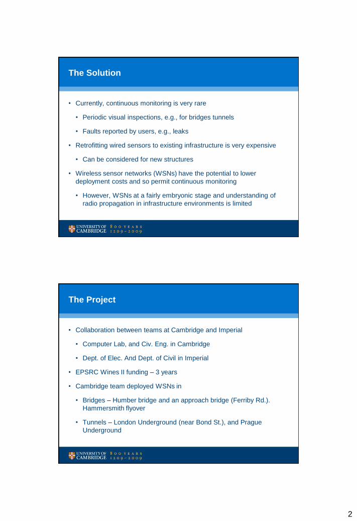
• Currently, continuous monitoring is very rare
• Periodic visual inspections, e.g., for bridges tunnels
• Faults reported by users, e.g., leaks
• Retrofitting wired sensors to existing infrastructure is very expensive
• Can be considered for new structures
• Wireless sensor networks (WSNs) have the potential to lower
deployment costs and so permit continuous monitoring
• However, WSNs at a fairly embryonic stage and understanding of
radio propagation in infrastructure environments is limited
The Project
• Collaboration between teams at Cambridge and Imperial
• Computer Lab, and Civ. Eng. in Cambridge
• Dept. of Elec. And Dept. of Civil in Imperial
• EPSRC Wines II funding – 3 years
• Cambridge team deployed WSNs in
• Bridges – Humber bridge and an approach bridge (Ferriby Rd.).
Hammersmith flyover
• Tunnels – London Underground (near Bond St.), and Prague
Underground
3
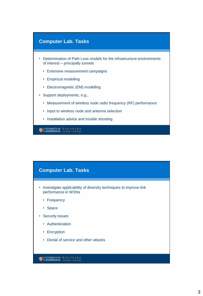
Computer Lab. Tasks
• Determination of Path Loss models for the infrastructure environments
of interest – principally tunnels
• Extensive measurement campaigns
• Empirical modelling
• Electromagnetic (EM) modelling
• Support deployments, e.g.,
• Measurement of wireless node radio frequency (RF) performance
• Input to wireless node and antenna selection
• Installation advice and trouble shooting
Computer Lab. Tasks
• Investigate applicability of diversity techniques to improve link
performance in WSNs
• Frequency
• Space
• Security issues
• Authentication
• Encryption
• Denial of service and other attacks
4
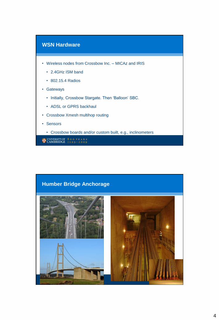
WSN Hardware
• Wireless nodes from Crossbow Inc. – MICAz and IRIS
• 2.4GHz ISM band
• 802.15.4 Radios
• Gateways
• Initially, Crossbow Stargate. Then ‘Balloon’ SBC.
• ADSL or GPRS backhaul
• Crossbow Xmesh multihop routing
• Sensors
• Crossbow boards and/or custom built, e.g., inclinometers
Humber Bridge Anchorage

5
Anchorage Deployment –
RH and temperature monitoring
• 12 node network
• 10 nodes measure RH and temperature
using off-the-shelf hardware
• 1 node acts as a relay
• 1 node measures inclination of the splay
saddle
• Gateway is connected to the Internet via
ADSL
• http://www.bridgeforum.com/humber/
Ferriby Road Bridge
6
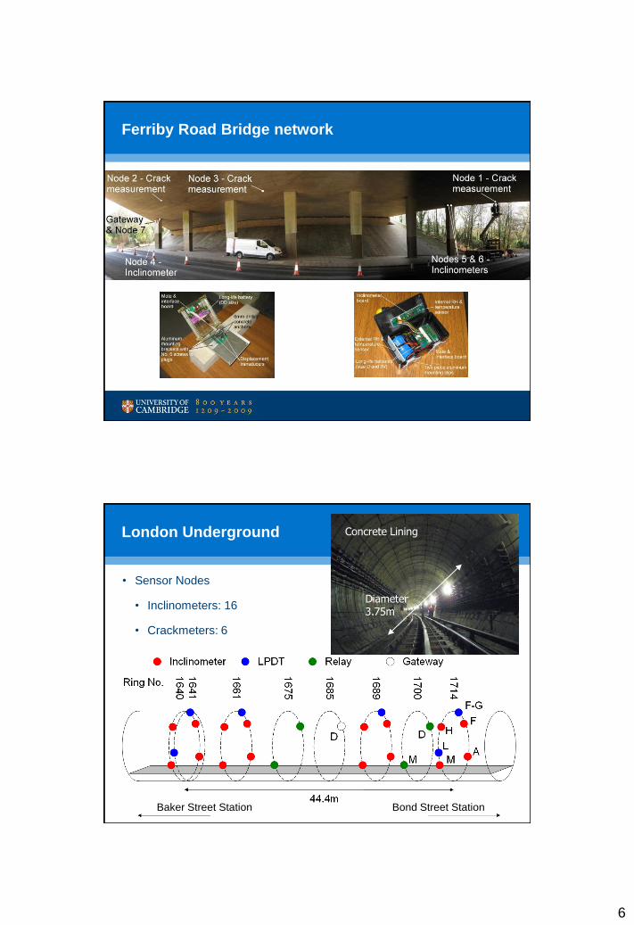
Ferriby Road Bridge network
London Underground
• Sensor Nodes
• Inclinometers: 16
• Crackmeters: 6
Diameter 3.75m
Concrete Lining
Bond Street Station Baker Street Station
7
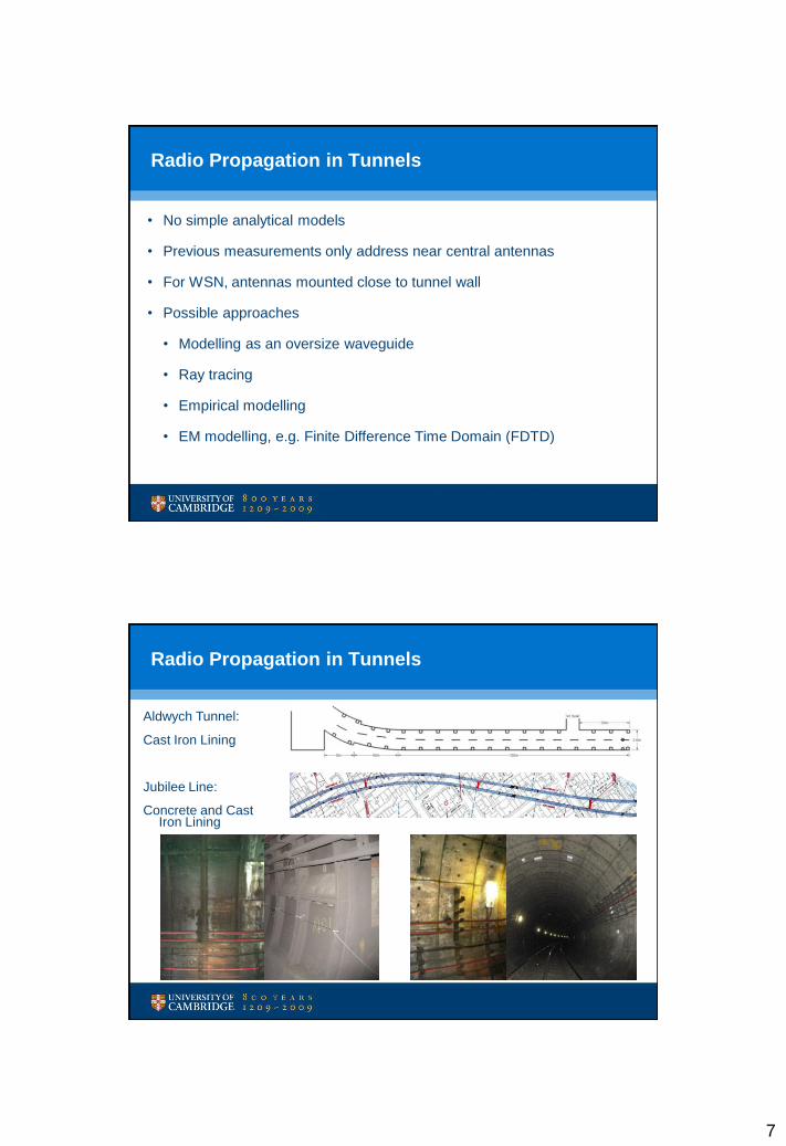
Radio Propagation in Tunnels
Expanded Concrete Segmental Lining
• No simple analytical models
• Previous measurements only address near central antennas
• For WSN, antennas mounted close to tunnel wall
• Possible approaches
• Modelling as an oversize waveguide
• Ray tracing
• Empirical modelling
• EM modelling, e.g. Finite Difference Time Domain (FDTD)
Aldwych Tunnel:
Cast Iron Lining
Jubilee Line:
Concrete and Cast Iron Lining
Radio Propagation in Tunnels
Cast Iron Lining Expanded Concrete Segmental Lining
8
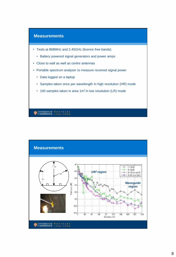
Measurements
• Tests at 868MHz and 2.45GHz (licence free bands)
• Battery powered signal generators and power amps
• Close to wall as well as centre antennas
• Portable spectrum analyser to measure received signal power
• Data logged on a laptop
• Samples taken once per wavelength in high resolution (HR) mode
• 100 samples taken in area 1m2 in low resolution (LR) mode
Measurements
1/R2 region
Waveguide
region
9
Comparisons
Factor Comparative Path Loss Performance
Antenna Position Centre to Centre (CC) > All other Side cases (SS)
Operating Frequency CC case: 868MHz > 2.45 GHz
SS case: 868MHz ≈ 2.45GHz
Material Cast Iron > Concrete
Course Straight ≈ Curved
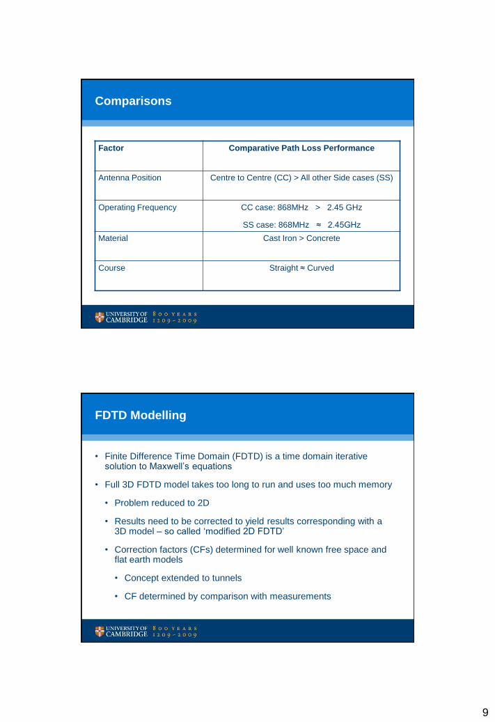
FDTD Modelling
• Finite Difference Time Domain (FDTD) is a time domain iterative solution to Maxwell’s equations
• Full 3D FDTD model takes too long to run and uses too much memory
• Problem reduced to 2D
• Results need to be corrected to yield results corresponding with a 3D model – so called ‘modified 2D FDTD’
• Correction factors (CFs) determined for well known free space and flat earth models
• Concept extended to tunnels
• CF determined by comparison with measurements
10
FDTD Modelling - Tunnel
• Comparison of modified 2D FDTD with measurements
CC (+20dB)
SS (-20dB)
1/R2 region
Waveguide
region
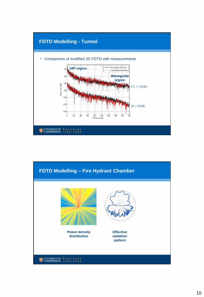
FDTD Modelling – Fire Hydrant Chamber
Power density
distribution
Effective
radiation
pattern

11
Current ways to Overcome Path Loss
• Increase transmit power
• Battery life penalty
• Improve receiver sensitivity
• Cost implications
• Relay/multihop networks
• Cost, installation time
• Increase antenna gain
• Size, cost, robustness issues
Antennas
58mm 215mm
42mm
12
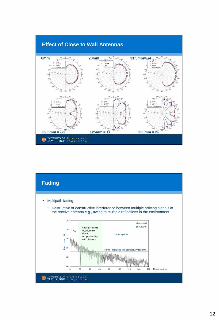
Effect of Close to Wall Antennas
6mm
62.5mm = l/2 125mm = 1l 250mm = 2l
31.5mm=l/4 20mm
Fading
• Multipath fading
• Destructive or constructive interference between multiple arriving signals at the receive antenna e.g., owing to multiple reflections in the environment
Distance / m
-100
-80
-60
-40
-20
0
0 20 40 60 80 100 120 140 160
Fading – some
locations no
signal,
inc. probability
with distance
No reception
Power required to successfully receive Pa
th L
oss / d
B
Measured
Simulation
OK

13
Fading
• Dependent on the environment – geometry, materials
• Can be modelled stochastically – difficult to predict exact location
• Fade positions static in a static environment
• Possibly solutions include frequency or space diversity
Empty People
Moving
Frequency Diversity
• Measurements conducted every 10m in 90m cast iron lined tunnel
• Measurements of received signal measured on 32 freq. channels,
5MHz spacing in 2.4GHz ISM band

14
Frequency Diversity (FD)
• Potential diversity gain quantified using correlation coefficient (CC)
• Values <0.7 indicate worthwhile gain
0 2 4 6 8 10 12 14 16 180.3
0.4
0.5
0.6
0.7
0.8
0.9
1
Channel Spacing
Avera
ge C
CC
SSS Measurement
SOS MeasurementCC • Hopping by 1 channel gives
reasonable FD gain
• FD gain increases with
channel separation
• Antennas on Same side
(SSS) of tunnel wall
experience less FD gain
than antennas on opposite
side (SOS)
Frequency Diversity (FD)
• Potential diversity gain quantified using correlation coefficient (CC)
• Values <0.7 indicate worthwhile gain
CC • FH gain decreases with
distance
• SOS in general experience
greater FD gain than SSS
0 10 20 30 40 50 60 70 80 900.3
0.4
0.5
0.6
0.7
0.8
0.9
1
Distance (m)
Avera
ge C
CC
SSS Measurement
SOS Measurement
15
Frequency Diversity (FD)
• FD has the potential to achieve diversity gain in the tunnel
environment
• Use of FD will improve link reliability and so ease deployment
problems
• No additional hardware required, but will make media access control
(MAC) layer more complicated
• Will give some immunity to radio frequency (RF) interference
• We will also be investigating the use of space diversity (SD)
Conclusions
• Use of WSN speeds up deployment but raises question of reliability
• Propagation knowledge important when planning deployment
• Lack of models for infrastructure deployments
• Antenna gain, radiation pattern and location important
• Fading a problem
• Difficult to accurately predict
• Frequency Diversity may be applicable in some environments
• Need for planning tools to assist in the deployment procedure, e.g.,
• To optimise placement of relay nodes