Wireless digital communication - MIT OpenCourseWare · PDF fileWireless digital communication...
61
Chapter 9 Wireless digital communication 9.1 Introduction This chapter provides a brief treatment of wireless digital communication systems. More exten- sive treatments are found in many texts, particularly [32] and [9] As the name suggests, wireless systems operate via transmission through space rather than through a wired connection. This has the advantage of allowing users to make and receive calls almost anywhere, including while in motion. Wireless communication is sometimes called mobile communication since many of the new technical issues arise from motion of the transmitter or receiver. There are two major new problems to be addressed in wireless that do not arise with wires. The first is that the communication channel often varies with time. The second is that there is often interference between multiple users. In previous chapters, modulation and coding techniques have been viewed as ways to combat the noise on communication channels. In wireless systems, these techniques must also combat time-variation and interference. This will cause major changes both in the modeling of the channel and the type of modulation and coding. Wireless communication, despite the hype of the popular press, is a field that has been around for over a hundred years, starting around 1897 with Marconi’s successful demonstrations of wireless telegraphy. By 1901, radio reception across the Atlantic Ocean had been established, illustrating that rapid progress in technology has also been around for quite a while. In the intervening hundred years, many types of wireless systems have flourished, and often later disappeared. For example, television transmission, in its early days, was broadcast by wireless radio transmitters, which is increasingly being replaced by cable or satellite transmission. Similarly, the point- to-point microwave circuits that formerly constituted the backbone of the telephone network are being replaced by optical fiber. In the first example, wireless technology became outdated when a wired distribution network was installed; in the second, a new wired technology (optical fiber) replaced the older wireless technology. The opposite type of example is occurring today in telephony, where cellular telephony is partially replacing wireline telephony, particularly in parts of the world where the wired network is not well developed. The point of these examples is that there are many situations in which there is a choice between wireless and wire technologies, and the choice often changes when new technologies become available. Cellular networks will be emphasized in this chapter, both because they are of great current interest and also because they involve a relatively simple architecture within which most of the physical layer communication aspects of wireless systems can be studied. A cellular network 305 Cite as: Robert Gallager, course materials for 6.450 Principles of Digital Communications I, Fall 2006. MIT OpenCourseWare (http://ocw.mit.edu/), Massachusetts Institute of Technology. Downloaded on [DD Month YYYY].
Transcript of Wireless digital communication - MIT OpenCourseWare · PDF fileWireless digital communication...
Chapter 9
Wireless digital communication
9.1 Introduction
This chapter provides a brief treatment of wireless digital communication systems. More extensive treatments are found in many texts, particularly [32] and [9] As the name suggests, wireless systems operate via transmission through space rather than through a wired connection. This has the advantage of allowing users to make and receive calls almost anywhere, including while in motion. Wireless communication is sometimes called mobile communication since many of the new technical issues arise from motion of the transmitter or receiver.
There are two major new problems to be addressed in wireless that do not arise with wires. The first is that the communication channel often varies with time. The second is that there is often interference between multiple users. In previous chapters, modulation and coding techniques have been viewed as ways to combat the noise on communication channels. In wireless systems, these techniques must also combat time-variation and interference. This will cause major changes both in the modeling of the channel and the type of modulation and coding.
Wireless communication, despite the hype of the popular press, is a field that has been around for over a hundred years, starting around 1897 with Marconi’s successful demonstrations of wireless telegraphy. By 1901, radio reception across the Atlantic Ocean had been established, illustrating that rapid progress in technology has also been around for quite a while. In the intervening hundred years, many types of wireless systems have flourished, and often later disappeared. For example, television transmission, in its early days, was broadcast by wireless radio transmitters, which is increasingly being replaced by cable or satellite transmission. Similarly, the point-to-point microwave circuits that formerly constituted the backbone of the telephone network are being replaced by optical fiber. In the first example, wireless technology became outdated when a wired distribution network was installed; in the second, a new wired technology (optical fiber) replaced the older wireless technology. The opposite type of example is occurring today in telephony, where cellular telephony is partially replacing wireline telephony, particularly in parts of the world where the wired network is not well developed. The point of these examples is that there are many situations in which there is a choice between wireless and wire technologies, and the choice often changes when new technologies become available.
Cellular networks will be emphasized in this chapter, both because they are of great current interest and also because they involve a relatively simple architecture within which most of the physical layer communication aspects of wireless systems can be studied. A cellular network
305
Cite as: Robert Gallager, course materials for 6.450 Principles of Digital Communications I, Fall 2006. MIT OpenCourseWare (http://ocw.mit.edu/), Massachusetts Institute of Technology. Downloaded on [DD Month YYYY].
� �
�� � ��� ��
306 CHAPTER 9. WIRELESS DIGITAL COMMUNICATION
consists of a large number of wireless subscribers with cellular telephones (cell phones) that can be used in cars, buildings, streets, etc. There are also a number of fixed base stations arranged to provide wireless electromagnetic communication with arbitrarily located cell phones.
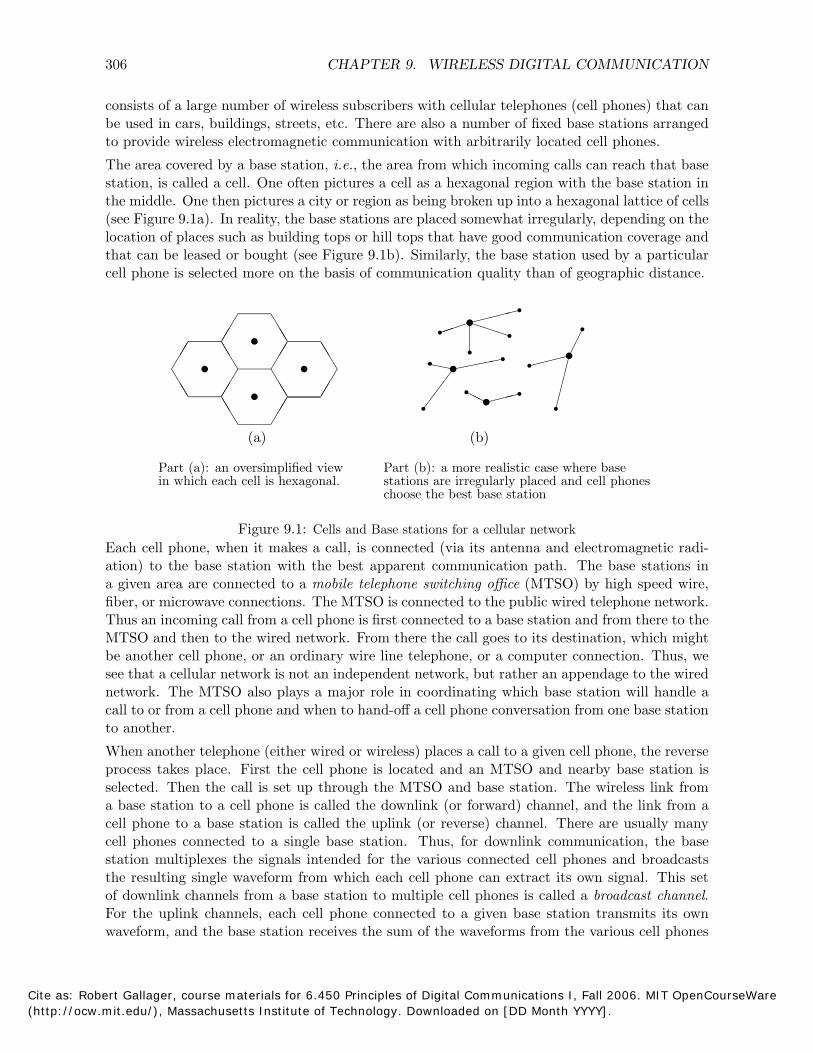
The area covered by a base station, i.e., the area from which incoming calls can reach that base station, is called a cell. One often pictures a cell as a hexagonal region with the base station in the middle. One then pictures a city or region as being broken up into a hexagonal lattice of cells (see Figure 9.1a). In reality, the base stations are placed somewhat irregularly, depending on the location of places such as building tops or hill tops that have good communication coverage and that can be leased or bought (see Figure 9.1b). Similarly, the base station used by a particular cell phone is selected more on the basis of communication quality than of geographic distance.
� � ����������� � �� � �� � � ���
��� �
��� �
�� � ��� � ����� ����
� � � � � ���
���� �
���� ��
�� � �� �� ��
���(a) (b)
Part (a): an oversimplified view Part (b): a more realistic case where base in which each cell is hexagonal. stations are irregularly placed and cell phones
choose the best base station
Figure 9.1: Cells and Base stations for a cellular network Each cell phone, when it makes a call, is connected (via its antenna and electromagnetic radiation) to the base station with the best apparent communication path. The base stations in a given area are connected to a mobile telephone switching office (MTSO) by high speed wire, fiber, or microwave connections. The MTSO is connected to the public wired telephone network. Thus an incoming call from a cell phone is first connected to a base station and from there to the MTSO and then to the wired network. From there the call goes to its destination, which might be another cell phone, or an ordinary wire line telephone, or a computer connection. Thus, we see that a cellular network is not an independent network, but rather an appendage to the wired network. The MTSO also plays a major role in coordinating which base station will handle a call to or from a cell phone and when to hand-off a cell phone conversation from one base station to another.
When another telephone (either wired or wireless) places a call to a given cell phone, the reverse process takes place. First the cell phone is located and an MTSO and nearby base station is selected. Then the call is set up through the MTSO and base station. The wireless link from a base station to a cell phone is called the downlink (or forward) channel, and the link from a cell phone to a base station is called the uplink (or reverse) channel. There are usually many cell phones connected to a single base station. Thus, for downlink communication, the base station multiplexes the signals intended for the various connected cell phones and broadcasts the resulting single waveform from which each cell phone can extract its own signal. This set of downlink channels from a base station to multiple cell phones is called a broadcast channel. For the uplink channels, each cell phone connected to a given base station transmits its own waveform, and the base station receives the sum of the waveforms from the various cell phones
Cite as: Robert Gallager, course materials for 6.450 Principles of Digital Communications I, Fall 2006. MIT OpenCourseWare (http://ocw.mit.edu/), Massachusetts Institute of Technology. Downloaded on [DD Month YYYY].
9.1. INTRODUCTION 307
plus noise. The base station must then separate and detect the signals from each cell phone and pass the resulting binary streams to the MTSO. This set of uplink channels to a given base station is called a multiaccess channel.
Early cellular systems were analog. They operated by directly modulating a voice waveform on a carrier and transmitting it. Different cell phones in the same cell were assigned different modulation frequencies, and adjacent cells used different sets of frequencies. Cells sufficiently far away from each other could reuse the same set of frequencies with little danger of interference.
All of the newer cellular systems are digital (i.e., use a binary interface), and thus, in principle, can be used for voice or data. Since these cellular systems, and their standards, originally focused on telephony, the current data rates and delays in cellular systems are essentially determined by voice requirements. At present, these systems are still mostly used for telephony, but both the capability to send data and the applications for data are rapidly increasing. Also the capabilities to transmit data at higher rates than telephony rates are rapidly being added to cellular systems.
As mentioned above, there are many kinds of wireless systems other than cellular. First there are the broadcast systems such as AM radio, FM radio, TV, and paging systems. All of these are similar to the broadcast part of cellular networks, although the data rates, the size of the areas covered by each broadcasting node, and the frequency ranges are very different.
In addition, there are wireless LANs (local area networks). These are designed for much higher data rates than cellular systems, but otherwise are somewhat similar to a single cell of a cellular system. These are designed to connect PC’s, shared peripheral devices, large computers, etc. within an office building or similar local environment. There is little mobility expected in such systems and their major function is to avoid stringing a maze of cables through an office building. The principal standards for such networks are the 802.11 family of IEEE standards. There is a similar even smaller-scale standard called Bluetooth whose purpose is to reduce cabling and simplify transfers between office and hand held devices.
Finally, there is another type of LAN called an ad hoc network. Here, instead of a central node (base station) through which all traffic flows, the nodes are all alike. These networks organize themselves into links between various pairs of nodes and develop routing tables using these links. The network layer issues of routing, protocols, and shared control are of primary concern for ad hoc networks; this is somewhat disjoint from our focus here on physical-layer communication issues.
One of the most important questions for all of these wireless systems is that of standardization. Some types of standardization are mandated by the Federal Communication Commission (FCC) in the USA and corresponding agencies in other countries. This has limited the available bandwidth for conventional cellular communication to three frequency bands, one around 0.9 gH, another around 1.9 gH, and the other around 5.8 gH. Other kinds of standardization are important since users want to use their cell phones over national and international areas. There are three well established mutually incompatible major types of digital cellular systems. One is the GSM system,1 which was standardized in Europe and is now used worldwide, another is a TDM (Time Division Modulation) standard developed in the U.S, and a third is CDMA (Code Division Multiple Access). All of these are evolving and many newer systems with a dizzying array of new features are constantly being introduced. Many cell phones can switch between multiple modes as a partial solution to these incompatibility issues.
1GSM stands for Groupe Speciale Mobile or Global Systems for Mobile Communication, but the acronym is far better known and just as meaningful as the words.
Cite as: Robert Gallager, course materials for 6.450 Principles of Digital Communications I, Fall 2006. MIT OpenCourseWare (http://ocw.mit.edu/), Massachusetts Institute of Technology. Downloaded on [DD Month YYYY].

308 CHAPTER 9. WIRELESS DIGITAL COMMUNICATION
This chapter will focus primarily on CDMA, partly because so many newer systems are using this approach, and partly because it provides an excellent medium for discussing communication principles. GSM and TDM will be discussed briefly, but the issues of standardization are so centered on non-technological issues and so rapidly changing that they will not be discussed further.
In thinking about wireless LAN’s and cellular telephony, an obvious question is whether they will some day be combined into one network. The use of data rates compatible with voice rates already exists in the cellular network, and the possibility of much higher data rates already exists in wireless LANs, so the question is whether very high data rates are commercially desirable for standardized cellular networks. The wireless medium is a much more difficult medium for communication than the wired network. The spectrum available for cellular systems is quite limited, the interference level is quite high, and rapid growth is increasing the level of interference. Adding higher data rates will exacerbate this interference problem even more. In addition, the display on hand held devices is small, limiting the amount of data that can be presented and suggesting that many applications of such devices do not need very high data rates. Thus it is questionable whether very high-speed data for cellular networks is necessary or desirable in the near future. On the other hand, there is intense competition between cellular providers, and each strives to distinguish their service by new features requiring increased data rates.
Subsequent sections begin the study of the technological aspects of wireless channels, focusing primarily on cellular systems. Section 9.2 looks briefly at the electromagnetic properties that propagate signals from transmitter to receiver. Section 9.3 then converts these detailed electromagnetic models into simpler input/output descriptions of the channel. These input/output models can be characterized most simply as linear time-varying filter models.
The input/output model above views the input, the channel properties, and the output at passband. Section 9.4 then finds the baseband equivalent for this passband view of the channel. It turns out that the channel can then be modeled as a complex baseband linear time-varying filter. Finally, in section 9.5, this deterministic baseband model is replaced by a stochastic model.
The remainder of the chapter then introduces various issues of communication over such a stochastic baseband channel. Along with modulation and detection in the presence of noise, we also discuss channel measurement, coding, and diversity. The chapter ends with a brief case study of the CDMA cellular standard, IS95.
9.2 Physical modeling for wireless channels
Wireless channels operate via electromagnetic radiation from transmitter to receiver. In principle, one could solve Maxwell’s equations for the given transmitted signal to find the electromagnetic field at the receiving antenna. This would have to account for the reflections from nearby buildings, vehicles, and bodies of land and water. Objects in the line of sight between transmitter and receiver would also have to be accounted for.
The wavelength Λ(f) of electromagnetic radiation at any given frequency f is given by Λ = c/f , where c = 3 × 10⁸ meters per second is the velocity of light. The wavelength in the bands allocated for cellular communication thus lies between 0.05 and 0.3 meters. To calculate the electromagnetic field at a receiver, the locations of the receiver and the obstructions would have to be known within sub-meter accuracies. The electromagnetic field equations therefore appear
Cite as: Robert Gallager, course materials for 6.450 Principles of Digital Communications I, Fall 2006. MIT OpenCourseWare (http://ocw.mit.edu/), Massachusetts Institute of Technology. Downloaded on [DD Month YYYY].
9.2. PHYSICAL MODELING FOR WIRELESS CHANNELS 309
to be unreasonable to solve, especially on the fly for moving users. Thus, electromagnetism cannot be used to characterize wireless channels in detail, but it will provide understanding about the underlying nature of these channels.
One important question is where to place base stations, and what range of power levels are then necessary on the downlinks and uplinks. To a great extent, this question must be answered experimentally, but it certainly helps to have a sense of what types of phenomena to expect. Another major question is what types of modulation techniques and detection techniques look promising. Here again, a sense of what types of phenomena to expect is important, but the information will be used in a different way. Since cell phones must operate under a wide variety of different conditions, it will make sense to view these conditions probabilistically. Before developing such a stochastic model for channel behavior, however, we first explore the gross characteristics of wireless channels by looking at several highly idealized models.
9.2.1 Free space, fixed transmitting and receiving antennas
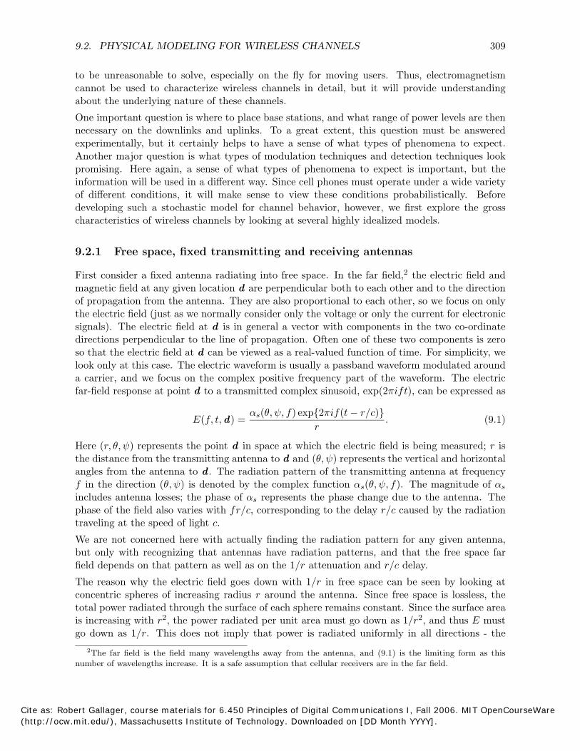
First consider a fixed antenna radiating into free space. In the far field,2 the electric field and magnetic field at any given location d are perpendicular both to each other and to the direction of propagation from the antenna. They are also proportional to each other, so we focus on only the electric field (just as we normally consider only the voltage or only the current for electronic signals). The electric field at d is in general a vector with components in the two co-ordinate directions perpendicular to the line of propagation. Often one of these two components is zero so that the electric field at d can be viewed as a real-valued function of time. For simplicity, we look only at this case. The electric waveform is usually a passband waveform modulated around a carrier, and we focus on the complex positive frequency part of the waveform. The electric far-field response at point d to a transmitted complex sinusoid, exp(2πift), can be expressed as
E(f, t, d) = αs(θ, ψ, f) exp{2πif(t − r/c)}
. (9.1) r
Here (r, θ, ψ) represents the point d in space at which the electric field is being measured; r is the distance from the transmitting antenna to d and (θ, ψ) represents the vertical and horizontal angles from the antenna to d . The radiation pattern of the transmitting antenna at frequency f in the direction (θ, ψ) is denoted by the complex function αs(θ, ψ, f). The magnitude of αs
includes antenna losses; the phase of αs represents the phase change due to the antenna. The phase of the field also varies with fr/c, corresponding to the delay r/c caused by the radiation traveling at the speed of light c.
We are not concerned here with actually finding the radiation pattern for any given antenna, but only with recognizing that antennas have radiation patterns, and that the free space far field depends on that pattern as well as on the 1/r attenuation and r/c delay.
The reason why the electric field goes down with 1/r in free space can be seen by looking at concentric spheres of increasing radius r around the antenna. Since free space is lossless, the total power radiated through the surface of each sphere remains constant. Since the surface area is increasing with r2, the power radiated per unit area must go down as 1/r2, and thus E must go down as 1/r. This does not imply that power is radiated uniformly in all directions - the
2The far field is the field many wavelengths away from the antenna, and (9.1) is the limiting form as this number of wavelengths increase. It is a safe assumption that cellular receivers are in the far field.
Cite as: Robert Gallager, course materials for 6.450 Principles of Digital Communications I, Fall 2006. MIT OpenCourseWare (http://ocw.mit.edu/), Massachusetts Institute of Technology. Downloaded on [DD Month YYYY].
∫ ∫
∫
310 CHAPTER 9. WIRELESS DIGITAL COMMUNICATION
radiation pattern is determined by the transmitting antenna. As seen later, this r−2 reduction of power with distance is sometimes invalid when there are obstructions to free space propagation.
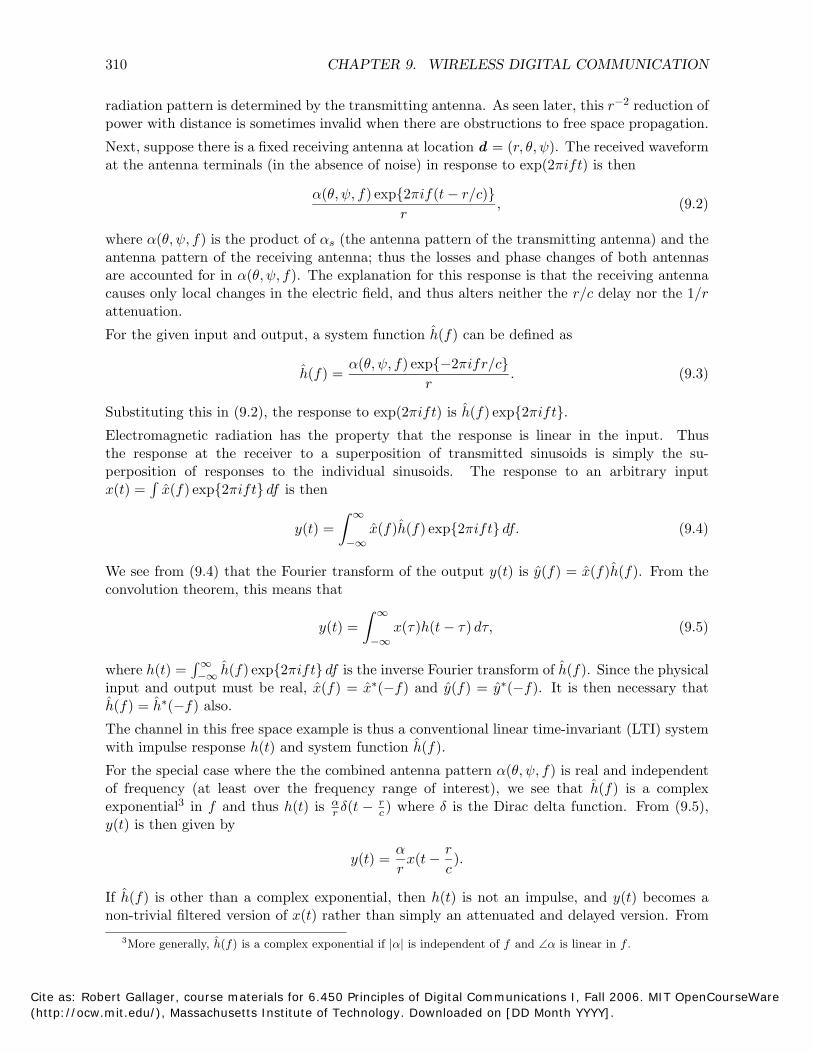
Next, suppose there is a fixed receiving antenna at location d = (r, θ, ψ). The received waveform at the antenna terminals (in the absence of noise) in response to exp(2πift) is then
α(θ, ψ, f) exp{2πif(t − r/c)}, (9.2)
r
where α(θ, ψ, f) is the product of αs (the antenna pattern of the transmitting antenna) and the antenna pattern of the receiving antenna; thus the losses and phase changes of both antennas are accounted for in α(θ, ψ, f). The explanation for this response is that the receiving antenna causes only local changes in the electric field, and thus alters neither the r/c delay nor the 1/r attenuation.
For the given input and output, a system function h(f) can be defined as
h(f) = α(θ, ψ, f) exp{−2πifr/c}
. (9.3) r
Substituting this in (9.2), the response to exp(2πift) is h(f) exp{2πift}. Electromagnetic radiation has the property that the response is linear in the input. Thus the response at the receiver to a superposition of transmitted sinusoids is simply the superposition of responses to the individual sinusoids. The response to an arbitrary input x(t) = x(f) exp{2πift} df is then
y(t) = ∞
x(f)h(f) exp{2πift} df. (9.4) −∞
We see from (9.4) that the Fourier transform of the output y(t) is y(f) = x(f)h(f). From the convolution theorem, this means that
y(t) = ∞
x(τ)h(t − τ) dτ, (9.5) −∞
where h(t) = ∫ ∞
h(f) exp{2πift} df is the inverse Fourier transform of h(f). Since the physical −∞input and output must be real, x(f) = x∗(−f) and y(f) = y∗(−f). It is then necessary that h(f) = h∗(−f) also.
The channel in this free space example is thus a conventional linear time-invariant (LTI) systemwith impulse response h(t) and system function h(f).
For the special case where the the combined antenna pattern α(θ, ψ, f) is real and independentof frequency (at least over the frequency range of interest), we see that h(f) is a complex
rexponential3 in f and thus h(t) is αr δ(t − c ) where δ is the Dirac delta function. From (9.5), y(t) is then given by
α r y(t) = x(t − ).
r c
If h(f) is other than a complex exponential, then h(t) is not an impulse, and y(t) becomes a non-trivial filtered version of x(t) rather than simply an attenuated and delayed version. From
3More generally, h(f) is a complex exponential if |α| is independent of f and ∠α is linear in f .
Cite as: Robert Gallager, course materials for 6.450 Principles of Digital Communications I, Fall 2006. MIT OpenCourseWare (http://ocw.mit.edu/), Massachusetts Institute of Technology. Downloaded on [DD Month YYYY].
9.2. PHYSICAL MODELING FOR WIRELESS CHANNELS 311
(9.4), however, y(t) only depends on h(f) over the frequency band where x(f) is non-zero. Thus it is common to model h(f) as a complex exponential (and thus h(t) as a scaled and shifted Dirac delta function) whenever h(f) is a complex exponential over the frequency band of use.
We will find in what follows that linearity is a good assumption for all the wireless channels to be considered, but that time invariance does not hold when either the antennas or reflecting objects are in relative motion.
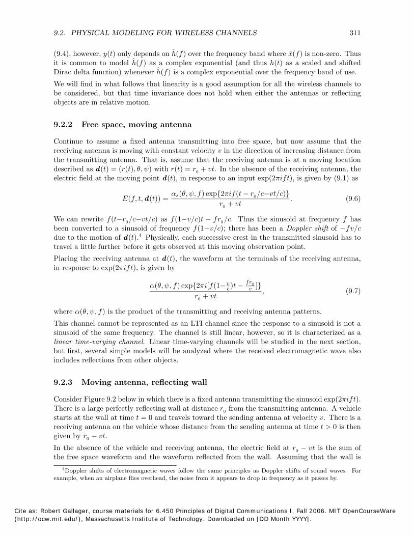
9.2.2 Free space, moving antenna
Continue to assume a fixed antenna transmitting into free space, but now assume that the receiving antenna is moving with constant velocity v in the direction of increasing distance from the transmitting antenna. That is, assume that the receiving antenna is at a moving location described as d(t) = (r(t), θ, ψ) with r(t) = r0 + vt. In the absence of the receiving antenna, the electric field at the moving point d(t), in response to an input exp(2πift), is given by (9.1) as
E(f, t, d(t)) = αs(θ, ψ, f) exp{2πif(t − r /c−vt/c)}
. (9.6)0
r0 + vt
We can rewrite f(t−r /c−vt/c) as f(1−v/c)t − fr /c. Thus the sinusoid at frequency f has0 0
been converted to a sinusoid of frequency f(1−v/c); there has been a Doppler shift of −fv/c due to the motion of d(t).4 Physically, each successive crest in the transmitted sinusoid has to travel a little further before it gets observed at this moving observation point.
Placing the receiving antenna at d(t), the waveform at the terminals of the receiving antenna, in response to exp(2πift), is given by
α(θ, ψ, f) exp{2πi[f(1−vc )t −
frc 0 ]}
, (9.7) r + vt0
where α(θ, ψ, f) is the product of the transmitting and receiving antenna patterns.
This channel cannot be represented as an LTI channel since the response to a sinusoid is not a sinusoid of the same frequency. The channel is still linear, however, so it is characterized as a linear time-varying channel. Linear time-varying channels will be studied in the next section, but first, several simple models will be analyzed where the received electromagnetic wave also includes reflections from other objects.
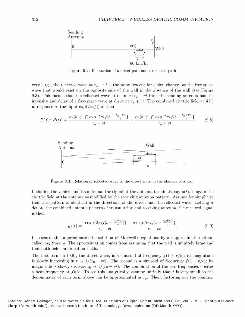
9.2.3 Moving antenna, reflecting wall
Consider Figure 9.2 below in which there is a fixed antenna transmitting the sinusoid exp(2πift). There is a large perfectly-reflecting wall at distance r0 from the transmitting antenna. A vehicle starts at the wall at time t = 0 and travels toward the sending antenna at velocity v. There is a receiving antenna on the vehicle whose distance from the sending antenna at time t > 0 is then given by r0 − vt.
In the absence of the vehicle and receiving antenna, the electric field at r0 − vt is the sum of the free space waveform and the waveform reflected from the wall. Assuming that the wall is
4Doppler shifts of electromagnetic waves follow the same principles as Doppler shifts of sound waves. For example, when an airplane flies overhead, the noise from it appears to drop in frequency as it passes by.
Cite as: Robert Gallager, course materials for 6.450 Principles of Digital Communications I, Fall 2006. MIT OpenCourseWare (http://ocw.mit.edu/), Massachusetts Institute of Technology. Downloaded on [DD Month YYYY].
312 CHAPTER 9. WIRELESS DIGITAL COMMUNICATION
Sending
�� ���� �� �� ����
�
Wall
Antenna
�
r(t)0
r0
60 km/hr
Figure 9.2: Illustration of a direct path and a reflected path
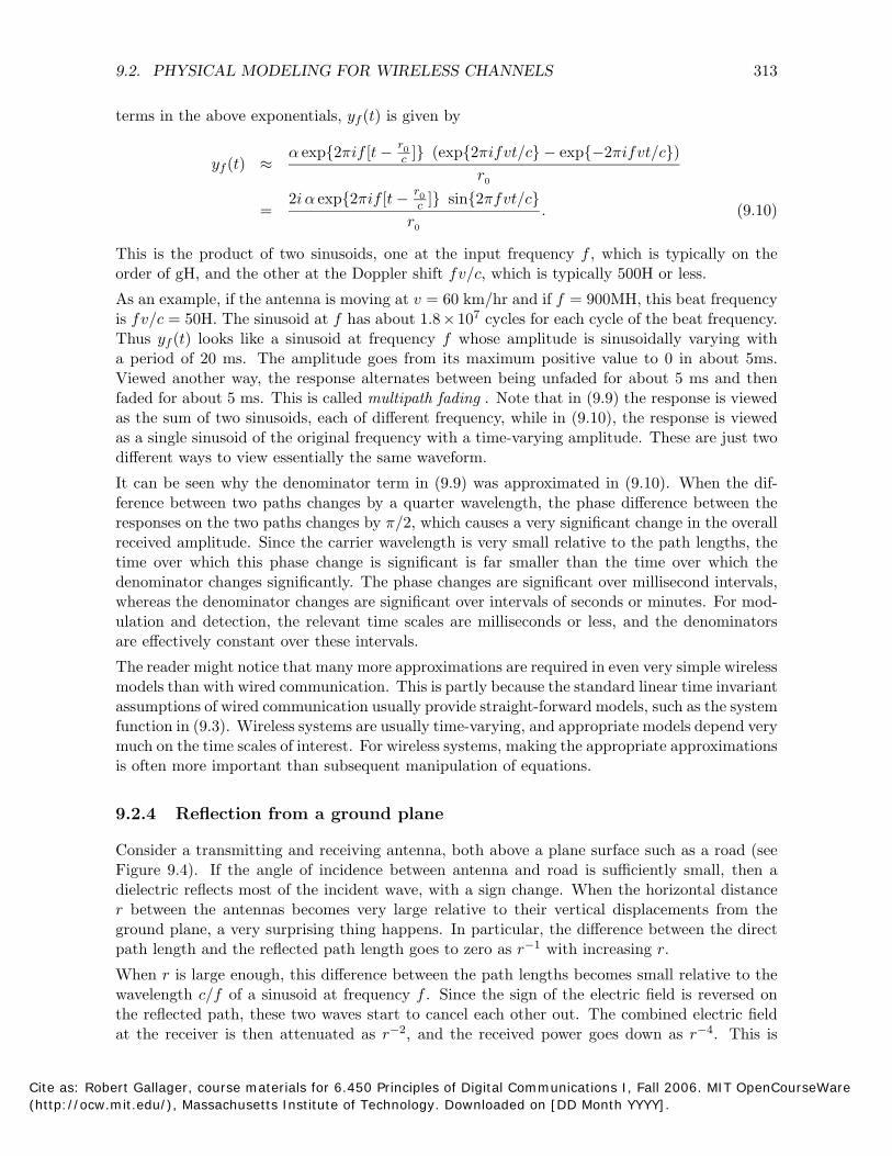
very large, the reflected wave at r0 − vt is the same (except for a sign change) as the free space wave that would exist on the opposite side of the wall in the absence of the wall (see Figure 9.3). This means that the reflected wave at distance r0 − vt from the sending antenna has the intensity and delay of a free-space wave at distance r0 + vt. The combined electric field at d(t) in response to the input exp(2πift) is then
0αs(θ, ψ, f) exp{2πif [t − r0−vt
αs(θ, ψ, f) exp{2πif [t − r +vt
E(f, t, d(t)) = r0 − vt
c ]} − r0 + vt
c ]}. (9.8)
Sending Antenna Wall
� �+vt
0 −vt
r0
Figure 9.3: Relation of reflected wave to the direct wave in the absence of a wall.
Including the vehicle and its antenna, the signal at the antenna terminals, say y(t), is again the electric field at the antenna as modified by the receiving antenna pattern. Assume for simplicity that this pattern is identical in the directions of the direct and the reflected wave. Letting α denote the combined antenna pattern of transmitting and receiving antenna, the received signal is then
0
yf (t) = α exp{2πif [t −
r0−c
vt ]} α exp{2πif [t − r +
c vt ]}
. (9.9) r0 − vt
− r + vt0
In essence, this approximates the solution of Maxwell’s equations by an approximate method called ray tracing. The approximation comes from assuming that the wall is infinitely large and that both fields are ideal far fields.
The first term in (9.9), the direct wave, is a sinusoid of frequency f(1 + v/c); its magnitude is slowly increasing in t as 1/(r0 − vt). The second is a sinusoid of frequency f(1 − v/c); its magnitude is slowly decreasing as 1/(r0 + vt). The combination of the two frequencies creates a beat frequency at fv/c. To see this analytically, assume initially that t is very small so the denominator of each term above can be approximated as r0 . Then, factoring out the common
Cite as: Robert Gallager, course materials for 6.450 Principles of Digital Communications I, Fall 2006. MIT OpenCourseWare (http://ocw.mit.edu/), Massachusetts Institute of Technology. Downloaded on [DD Month YYYY].
9.2. PHYSICAL MODELING FOR WIRELESS CHANNELS 313
terms in the above exponentials, yf (t) is given by
0
yf (t) α exp{2πif [t −
r ]} (exp{2πifvt/c} − exp{−2πifvt/c})c≈ r0
0
=2i α exp{2πif [t −
r ]} sin{2πfvt/c}. (9.10)c
r0
This is the product of two sinusoids, one at the input frequency f , which is typically on the order of gH, and the other at the Doppler shift fv/c, which is typically 500H or less.
As an example, if the antenna is moving at v = 60 km/hr and if f = 900MH, this beat frequency is fv/c = 50H. The sinusoid at f has about 1.8 × 10⁷ cycles for each cycle of the beat frequency. Thus yf (t) looks like a sinusoid at frequency f whose amplitude is sinusoidally varying with a period of 20 ms. The amplitude goes from its maximum positive value to 0 in about 5ms. Viewed another way, the response alternates between being unfaded for about 5 ms and then faded for about 5 ms. This is called multipath fading . Note that in (9.9) the response is viewed as the sum of two sinusoids, each of different frequency, while in (9.10), the response is viewed as a single sinusoid of the original frequency with a time-varying amplitude. These are just two different ways to view essentially the same waveform.
It can be seen why the denominator term in (9.9) was approximated in (9.10). When the difference between two paths changes by a quarter wavelength, the phase difference between the responses on the two paths changes by π/2, which causes a very significant change in the overall received amplitude. Since the carrier wavelength is very small relative to the path lengths, the time over which this phase change is significant is far smaller than the time over which the denominator changes significantly. The phase changes are significant over millisecond intervals, whereas the denominator changes are significant over intervals of seconds or minutes. For modulation and detection, the relevant time scales are milliseconds or less, and the denominators are effectively constant over these intervals.
The reader might notice that many more approximations are required in even very simple wireless models than with wired communication. This is partly because the standard linear time invariant assumptions of wired communication usually provide straight-forward models, such as the system function in (9.3). Wireless systems are usually time-varying, and appropriate models depend very much on the time scales of interest. For wireless systems, making the appropriate approximations is often more important than subsequent manipulation of equations.
9.2.4 Reflection from a ground plane
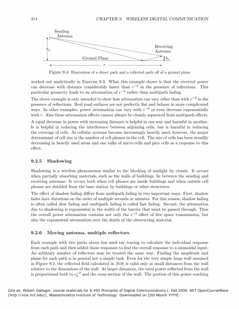
Consider a transmitting and receiving antenna, both above a plane surface such as a road (see Figure 9.4). If the angle of incidence between antenna and road is sufficiently small, then a dielectric reflects most of the incident wave, with a sign change. When the horizontal distance r between the antennas becomes very large relative to their vertical displacements from the ground plane, a very surprising thing happens. In particular, the difference between the direct path length and the reflected path length goes to zero as r−1 with increasing r.
When r is large enough, this difference between the path lengths becomes small relative to the wavelength c/f of a sinusoid at frequency f . Since the sign of the electric field is reversed on the reflected path, these two waves start to cancel each other out. The combined electric field at the receiver is then attenuated as r−2, and the received power goes down as r−4 . This is
Cite as: Robert Gallager, course materials for 6.450 Principles of Digital Communications I, Fall 2006. MIT OpenCourseWare (http://ocw.mit.edu/), Massachusetts Institute of Technology. Downloaded on [DD Month YYYY].
��������������������������������� ��
�
314 CHAPTER 9. WIRELESS DIGITAL COMMUNICATION
SendingAntenna
Receivinghs
����������������������
Antenna
� Ground Plane ��� ��hr
� r �
Figure 9.4: Illustration of a direct path and a reflected path off of a ground plane
worked out analytically in Exercise 9.3. What this example shows is that the received power can decrease with distance considerably faster than r−2 in the presence of reflections. This particular geometry leads to an attenuation of r−4 rather than multipath fading.
The above example is only intended to show how attenuation can vary other than with r−2 in the presence of reflections. Real road surfaces are not perfectly flat and behave in more complicated ways. In other examples, power attenuation can vary with r−6 or even decrease exponentially with r. Also these attenuation effects cannot always be cleanly separated from multipath effects.
A rapid decrease in power with increasing distance is helpful in one way and harmful in another. It is helpful in reducing the interference between adjoining cells, but is harmful in reducing the coverage of cells. As cellular systems become increasingly heavily used, however, the major determinant of cell size is the number of cell phones in the cell. The size of cells has been steadily decreasing in heavily used areas and one talks of micro cells and pico cells as a response to this effect.
9.2.5 Shadowing
Shadowing is a wireless phenomenon similar to the blocking of sunlight by clouds. It occurs when partially absorbing materials, such as the walls of buildings, lie between the sending and receiving antennas. It occurs both when cell phones are inside buildings and when outside cell phones are shielded from the base station by buildings or other structures.
The effect of shadow fading differs from multipath fading in two important ways. First, shadow fades have durations on the order of multiple seconds or minutes. For this reason, shadow fading is often called slow fading and multipath fading is called fast fading. Second, the attenuation due to shadowing is exponential in the width of the barrier that must be passed through. Thus the overall power attenuation contains not only the r−2 effect of free space transmission, but also the exponential attenuation over the depth of the obstructing material.
9.2.6 Moving antenna, multiple reflectors
Each example with two paths above has used ray tracing to calculate the individual response from each path and then added those responses to find the overall response to a sinusoidal input. An arbitrary number of reflectors may be treated the same way. Finding the amplitude and phase for each path is in general not a simple task. Even for the very simple large wall assumed in Figure 9.2, the reflected field calculated in (9.9) is valid only at small distances from the wall relative to the dimensions of the wall. At larger distances, the total power reflected from the wall is proportional both to r0
−2 and the cross section of the wall. The portion of this power reaching
Cite as: Robert Gallager, course materials for 6.450 Principles of Digital Communications I, Fall 2006. MIT OpenCourseWare (http://ocw.mit.edu/), Massachusetts Institute of Technology. Downloaded on [DD Month YYYY].
9.3. INPUT/OUTPUT MODELS OF WIRELESS CHANNELS 315
the receiver is proportional to (r0 − r(t))−2 . Thus the power attenuation from transmitter to receiver (for the reflected wave at large distances) is proportional to [r0(r0 − r(t)]−2 rather than to [2r0 − r(t)]−2 . This shows that ray tracing must be used with some caution. Fortunately, however, linearity still holds in these more complex cases.
Another type of reflection is known as scattering and can occur in the atmosphere or in reflections from very rough objects. Here the very large set of paths is better modeled as an integral over infinitesimally weak paths rather than as a finite sum.
Finding the amplitude of the reflected field from each type of reflector is important in determining the coverage, and thus the placement, of base stations, although ultimately experimentation is necessary. Studying this in more depth, however, would take us too far into electromagnetic theory and too far away from questions of modulation, detection, and multiple access. Thus we now turn our attention to understanding the nature of the aggregate received waveform, given a representation for each reflected wave. This means modeling the input/output behavior of a channel rather than the detailed response on each path.
9.3 Input/output models of wireless channels
This section shows how to view a channel consisting of an arbitrary collection of J electromagnetic paths as a more abstract input/output model. For the reflecting wall example, there is a direct path and one reflecting path, so J = 2. In other examples, there might be a direct path along with multiple reflected paths, each coming from a separate reflecting object. In many cases, the direct path is blocked and only indirect paths exist.
In many physical situations, the important paths are accompanied by other insignificant and highly attenuated paths. In these cases, the insignificant paths are omitted from the model and J denotes the number of remaining significant paths.
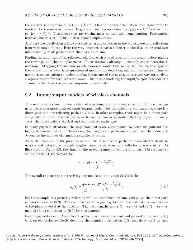
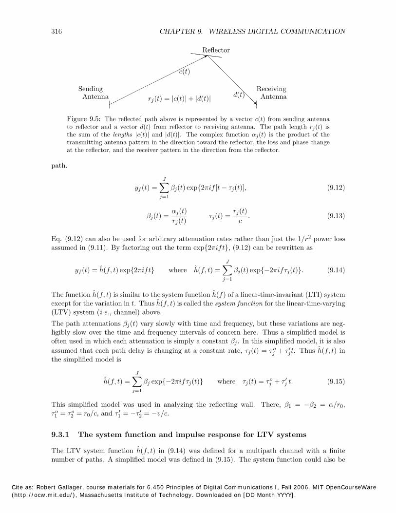
As in the examples of the previous section, the J significant paths are associated with attenuations and delays due to path lengths, antenna patterns, and reflector characteristics. As illustrated in Figure 9.5, the signal at the receiving antenna coming from path j in response to an input exp(2πift) is given by
αj exp{2πif [t − rj c (t) ]}
rj (t) .
The overall response at the receiving antenna to an input exp(2πift) is then
J rj (t) cyf (t) =
∑ αj exp{2πif [t − ]}. (9.11)
rj (t)j=1
For the example of a perfectly reflecting wall, the combined antenna gain α1 on the direct path is denoted as α in (9.9). The combined antenna gain α2 for the reflected path is −α because of the phase reversal at the reflector. The path lengths are r1(t) = r0 − vt and r2(t) = r0 + vt, making (9.11) equivalent to (9.9) for this example.
For the general case of J significant paths, it is more convenient and general to replace (9.11) with an expression explicitly denoting the complex attenuation βj (t) and delay τj (t) on each
Cite as: Robert Gallager, course materials for 6.450 Principles of Digital Communications I, Fall 2006. MIT OpenCourseWare (http://ocw.mit.edu/), Massachusetts Institute of Technology. Downloaded on [DD Month YYYY].
� �
∑
∑
∑
316 CHAPTER 9. WIRELESS DIGITAL COMMUNICATION
Reflector
c(t) �
����
����
����
�����
�
Sending �� Receiving
Antenna rj (t) = |c(t)| + |d(t)| d(t) ���
Antenna
Figure 9.5: The reflected path above is represented by a vector c(t) from sending antenna to reflector and a vector d(t) from reflector to receiving antenna. The path length rj (t) is the sum of the lengths |c(t)| and |d(t)|. The complex function αj (t) is the product of the transmitting antenna pattern in the direction toward the reflector, the loss and phase change at the reflector, and the receiver pattern in the direction from the reflector.
path.
J
yf (t) = βj (t) exp{2πif [t − τj (t)], (9.12) j=1
βj (t) = α
rj
j
((t
t
))
τj (t) = rj
c (t)
. (9.13)
Eq. (9.12) can also be used for arbitrary attenuation rates rather than just the 1/r2 power loss assumed in (9.11). By factoring out the term exp{2πift}, (9.12) can be rewritten as
J
yf (t) = h(f, t) exp{2πift} where h(f, t) = βj (t) exp{−2πifτj (t)}. (9.14) j=1
The function h(f, t) is similar to the system function h(f) of a linear-time-invariant (LTI) system except for the variation in t. Thus h(f, t) is called the system function for the linear-time-varying (LTV) system (i.e., channel) above.
The path attenuations βj (t) vary slowly with time and frequency, but these variations are negligibly slow over the time and frequency intervals of concern here. Thus a simplified model is often used in which each attenuation is simply a constant βj . In this simplified model, it is also assumed that each path delay is changing at a constant rate, τj(t) = τj
o + τj′t. Thus h(f, t) in
the simplified model is
J
h(f, t) = βj exp{−2πifτj (t)} where τj (t) = τjo + τj
′ t. (9.15) j=1
This simplified model was used in analyzing the reflecting wall. There, β1 = −β2 = α/r0, τ1
o = τ2 o = r0/c, and τ1
′ = −τ2′ = −v/c.
9.3.1 The system function and impulse response for LTV systems
The LTV system function h(f, t) in (9.14) was defined for a multipath channel with a finite number of paths. A simplified model was defined in (9.15). The system function could also be
Cite as: Robert Gallager, course materials for 6.450 Principles of Digital Communications I, Fall 2006. MIT OpenCourseWare (http://ocw.mit.edu/), Massachusetts Institute of Technology. Downloaded on [DD Month YYYY].
∫ ∫
∫ ∫
∫ [∫ ]
∫ [∫ ]
∫
9.3. INPUT/OUTPUT MODELS OF WIRELESS CHANNELS 317
generalized in a straight-forward way to a channel with a continuum of paths. More generally yet, if yf (t) is the response to the input exp{2πift}, then h(f, t) is defined as yf (t) exp{−2πift}. In this subsection, h(f, t) exp{2πift} is taken to be the response to exp{2πift} for each frequency f . The objective is then to find the response to an arbitrary input x(t). This will involve generalizing the well-known impulse response and convolution equation of LTI systems to the LTV case.
The key assumption in this generalization is the linearity of the system. That is, if y1(t) and y2(t) are the responses to x1(t) and x2(t) respectively, then α1y1(t) + α2y2(t) is the response to α1x1(t) + α2x2(t). This linearity follows from Maxwell’s equations5 .
Using linearity, the response to a superposition of complex sinusoids, say x(t) = ∞
x(f) exp{2πift} df , is −∞
y(t) = ∞
x(f)h(f, t) exp(2πift) df. (9.16) −∞
There is a temptation here to blindly imitate the theory of LTI systems and to confuse the Fourier transform of y(t), namely y(f), with x(f)h(f, t). This is wrong both logically and physically. It is wrong logically because x(f)h(f, t) is a function of t and f , whereas y(f) is a function only of f . It is wrong physically because Doppler shifts cause the response to x(f) exp(2πift) to contain multiple sinusoids around f rather than a single sinusoid at f . From the receiver’s viewpoint, y(f) at a given f depends on x(f) over a range of f around f .
Fortunately, (9.16) can still be used to derive a very satisfactory form of impulse response and convolution equation. Define the time-varying impulse response h(τ, t) as the inverse Fourier transform (in the time variable τ) of h(f, t), where t is viewed as a parameter. That is, for each t ∈ R,
h(τ, t) = ∞
h(f, t) exp(2πifτ) df h(f, t) = ∞
h(τ, t) exp(−2πifτ) dτ. (9.17) −∞ −∞
Intuitively, h(f, t) is regarded as a conventional LTI system function that is slowly changing with t and h(τ, t) is regarded as a channel impulse response (in τ) that is slowly changing with t. Substituting the second part of (9.17) into (9.16),
y(t) = ∞
x(f) ∞
h(τ, t) exp[2πif(t − τ)] dτ df. −∞ −∞
Interchanging the order of integration,6
y(t) = ∞
h(τ, t) ∞
x(f) exp[2πif(t − τ)] df dτ. −∞ −∞
Identifying the inner integral as x(t − τ), we get the convolution equation for LTV filters,
y(t) = ∞
x(t − τ)h(τ, t) dτ. (9.18) −∞
5Nonlinear effects can occur in high-power transmitting antennas, but we ignore that here. 6Questions about convergence and interchange of limits will be ignored in this section. This is reasonable since
the inputs and outputs of interest should be essentially time and frequency limited to the range of validity of the simplified multipath model.
Cite as: Robert Gallager, course materials for 6.450 Principles of Digital Communications I, Fall 2006. MIT OpenCourseWare (http://ocw.mit.edu/), Massachusetts Institute of Technology. Downloaded on [DD Month YYYY].

∫ ∫
∑ ∑
∑
318 CHAPTER 9. WIRELESS DIGITAL COMMUNICATION
This expression is really quite nice. It says that the effects of mobile transmitters and receivers, arbitrarily moving reflectors and absorbers, and all of the complexities of solving Maxwell’s equations, finally reduce to an input/output relation between transmit and receive antennas which is simply represented as the impulse response of an LTV channel filter. That is, h(τ, t) is the response at time t to an impulse at time t − τ . If h(τ, t) is a constant function of t, then h(τ, t), as a function of τ , is the conventional LTI impulse response.
This derivation applies for both real and complex inputs. The actual physical input x(t) at bandpass must be real, however, and for every real x(t), the corresponding output y(t) must also be real. This means that the LTV impulse response h(τ, t) must also be real. It then follows from (9.17) that h(−f, t) = h∗(f, t), which defines h(−f, t) in terms of h(f, t) for all f > 0.
There are many similarities between the results above for LTV filters and the conventional results for LTI filters. In both cases, the output waveform is the convolution of the input waveform with the impulse response; in the LTI case, y(t) = x(t − τ)h(τ) dτ , whereas in the LTV case, y(t) = x(t − τ)h(τ, t) dτ . In both cases, the system function is the Fourier transform of the impulse response; for LTI filters, h(τ) h(f) and for LTV filters h(τ, t) h(f, t), i.e., for each ↔ ↔ t the function h(f, t) (as a function of f) is the Fourier transform of h(τ, t) (as a function of τ). The most significant difference is that y(f) = h(f) x(f) in the LTI case, whereas in the LTV case, the corresponding statement says only that y(t) is the inverse Fourier transform of h(f, t)x(f).
It is important to realize that the Fourier relationship between the time-varying impulse response h(τ, t) and the time-varying system function h(f, t) is valid for any LTV system and does not depend on the simplified multipath model of (9.15). This simplified multipath model is valuable, however, in acquiring insight into how multipath and time-varying attenuation affect the transmitted waveform.
For the simplified model of (9.15), h(τ, t) can be easily derived from h(f, t) as
J
h(f, t) = βj exp{−2πifτj (t)} h(τ, t) = βj δ{τ − τj (t)}, (9.19)↔ j=1 j
where δ is the Dirac delta function. Substituting (9.19) into (9.18),
y(t) = βj x(t − τj (t)). (9.20) j
This says that the response at time t to an arbitrary input is the sum of the responses over all paths. The response on path j is simply the input, delayed by τj(t) and attenuated by βj . Note that both the delay and attenuation are evaluated at the time t at which the output is being measured.
The idealized, non-physical, impulses in (9.19) arise because of the tacit assumption that the attenuation and delay on each path are independent of frequency. It can be seen from (9.16) that h(f, t) affects the output only over the frequency band where x(f) is non-zero. If frequency independence holds over this band, it does no harm to assume it over all frequencies, leading to the above impulses. For typical relatively narrow-band applications, this frequency independence is usually a reasonable assumption.
Neither the general results about LTV systems nor the results for the multipath models of (9.14) and (9.15) provide much immediate insight into the nature of fading. The following
Cite as: Robert Gallager, course materials for 6.450 Principles of Digital Communications I, Fall 2006. MIT OpenCourseWare (http://ocw.mit.edu/), Massachusetts Institute of Technology. Downloaded on [DD Month YYYY].
∑
∑
∑
9.3. INPUT/OUTPUT MODELS OF WIRELESS CHANNELS 319
two subsections look at this issue, first for sinusoidal inputs, and then for general narrow-band inputs.
9.3.2 Doppler spread and coherence time
Assuming the simplified model of multipath fading in (9.15), the system function h(f, t) can be expressed as
J
h(f, t) = βj exp{−2πif(τj′ t + τj
o)}j=1
The rate of change of delay, τj′, on path j is related to the Doppler shift on path j at frequency
f by Dj = −fτj′, and thus h(f, t) can be expressed directly in terms of the Doppler shifts as
J
h(f, t) = βj exp{2πi(Djt − fτjo)}
j=1
The response to an input exp{2πift} is then
J
yf (t) = h(f, t) exp{2πift} = βj exp{2πi(f + Dj)t − fτjo} (9.21)
j=1
This is the sum of sinusoids around f ranging from f + Dmin to f + Dmax, where Dmin is the smallest of the Doppler shifts and Dmax is the largest. The terms −2πifτo are simply phases. j
The Doppler shifts Dj above can be positive or negative, but can be assumed to be small relative to the transmission frequency f . Thus yf (t) is a narrow band waveform whose bandwidth is the spread between Dmin and Dmax. This spread,
D = max Dj − min Dj (9.22)j j
is defined as the Doppler spread of the channel. The Doppler spread is a function of f (since all the Doppler shifts are functions of f), but it is usually viewed as a constant since it is approximately constant over any given frequency band of interest.
As shown above, the Doppler spread is the bandwidth of yf (t), but it is now necessary to be more specific about how to define fading. This will also lead to a definition of the coherence time of a channel.
The fading in (9.21) can be brought out more clearly by expressing h(f, t) in terms of its magnitude and phase, i.e., as |h(f, t)| ei∠h(f,t). The response to exp{2πift} is then
yf (t) = |h(f, t)| exp{2πift + i∠h(f, t)}. (9.23)
This expresses yf (t) as an amplitude term |h(f, t)| times a phase modulation of magnitude 1. This amplitude term h(f, t) is now defined as the fading amplitude of the channel at frequency |
ˆ|
f . As explained above, |h(f, t)| and ∠h(f, t) are slowly varying with t relative to exp{2πift}, so it makes sense to view |h(f, t)| as a slowly varying envelope, i.e., a fading envelope, around the received phase modulated sinusoid.
Cite as: Robert Gallager, course materials for 6.450 Principles of Digital Communications I, Fall 2006. MIT OpenCourseWare (http://ocw.mit.edu/), Massachusetts Institute of Technology. Downloaded on [DD Month YYYY].
∑
320 CHAPTER 9. WIRELESS DIGITAL COMMUNICATION
The fading amplitude can be interpreted more clearly in terms of the response �[yf (t)] to an actual real input sinusoid cos(2πft) = �[exp(2πift)]. Taking the real part of (9.23),
�[yf (t)] = |h(f, t)| cos[2πft + ∠h(f, t)].
The waveform �[yf (t)] oscillates at roughly the frequency f inside the slowly varying limits ±|h(f, t)|. This shows that|h(f, t)| is also the envelope, and thus the fading amplitude, of �[yf (t)] (at the given frequency f). This interpretation will be extended later to narrow band inputs around the frequency f .
We have seen from (9.21) that D is the bandwidth of yf (t), and it is also the bandwidth of �[yf (t)]. Assume initially that the Doppler shifts are centered around 0, i.e., that Dmax = −Dmin. Then h(f, t) is a baseband waveform containing frequencies between −D/2 and +D/2. The envelope of �[yf (t)], namely |h(f, t)|, is the magnitude of a waveform baseband limited to D/2. For the reflecting wall example, D1 = −D2, the Doppler spread is D = 2D1, and the envelope is | sin[2π(D/2)t]|. More generally, the Doppler shifts might be centered around some non-zero ∆ defined as the midpoint between minj Dj and maxj Dj . In this case, consider the frequency shifted system function ψ(f, t) defined as
J
ψ(f, t) = exp(−2πit∆) h(f, t) = βj exp{2πit(Dj−∆) − 2πifτjo} (9.24)
j=1
As a function of t, ψ(f, t) has bandwidth D/2. Since
|ψ(f, t)| = |e−2πi∆t h(f, t)| = |h(f, t)|,
the envelope of �[yf (t)] is the same as7 the magnitude of ψ(f, t), i.e., the magnitude of a waveform baseband limited to D/2. Thus this limit to D/2 is valid independent of the Doppler shift centering.
As an example, assume there is only one path and its Doppler shift is D1. Then h(f, t) is a complex sinusoid at frequency D1, but |h(f, t)| is a constant, namely |β1|. The Doppler spread is 0, the envelope is constant, and there is no fading. As another example, suppose the transmitter in the reflecting wall example is moving away from the wall. This decreases both of the Doppler shifts, but the difference between them, namely the Doppler spread, remains the same. The envelope |h(f, t)| then also remains the same. Both of these examples illustrate that it is the Doppler spread rather than the individual Doppler shifts that controls the envelope.
Define the coherence time Tcoh of the channel to be8
1 Tcoh = , (9.25)2D
This is one quarter of the wavelength of D/2 (the maximum frequency in ψ(f, t)) and one half the corresponding sampling interval. Since the envelope is |ψ(f, t)|, Tcoh serves as a crude
7Note that ψ(f, t), as a function of t, is baseband limited to D/2, whereas h(f, t) is limited to frequencies within D/2 of ∆ and yf (t) is limited to frequencies within D/2 of f+∆. It is rather surprising initially that all these waveforms have the same envelope. We focus on ψ(f, t) = e−2πif∆h(f, t) since this is the function that is baseband limited to D/2. Exercises 6.17 and 9.5 give additional insight and clarifying examples about the envelopes of real passband waveforms.
8Some authors define Tcoh as 1/(4D) and others as 1/D; these have the same order-of-magnitude interpretations.
Cite as: Robert Gallager, course materials for 6.450 Principles of Digital Communications I, Fall 2006. MIT OpenCourseWare (http://ocw.mit.edu/), Massachusetts Institute of Technology. Downloaded on [DD Month YYYY].
9.3. INPUT/OUTPUT MODELS OF WIRELESS CHANNELS 321
order-of-magnitude measure of the typical time interval for the envelope to change significantly. Since this envelope is the fading amplitude of the channel at frequency f , Tcoh is fundamentally interpreted as the order-of-magnitude duration of a fade at f . Since D is typically less than 1000H, Tcoh is typically greater than 1/2 msec.
Although the rapidity of changes in a baseband function cannot be specified solely in terms of its bandwidth, high bandwidth functions tend to change more rapidly than low bandwidth functions; the definition of coherence time captures this loose relationship. For the reflecting wall example, the envelope goes from its maximum value down to 0 over the period Tcoh; this is more or less typical of more general examples.
Crude though Tcoh might be as a measure of fading duration, it is an important parameter in describing wireless channels. It is used in waveform design, diversity provision, and channel measurement strategies. Later, when stochastic models are introduced for multipath, the relationship between fading duration and Tcoh will become sharper.
It is important to realize that Doppler shifts are linear in the input frequency, and thus Doppler spread is also. For narrow band inputs, the variation of Doppler spread with frequency is insignificant. When comparing systems in different frequency bands, however, the variation of D with frequency is important. For example, a system operating at 8 gH has a Doppler spread 8 times that of a 1 gH system and thus a coherence time 1/8th as large; fading is faster, with shorter fade durations, and channel measurements become outdated 8 times as fast.
9.3.3 Delay spread, and coherence frequency
Another important parameter of a wireless channel is the spread in delay between different paths. The delay spread L is defined as the difference between the path delay on the longest significant path and that on the shortest significant path. That is,
L = max [τj (t)] − min[τj (t)]. j j
The difference between path lengths is rarely greater than a few kilometers, so L is rarely more than several microseconds. Since the path delays τj (t) are changing with time, L can also change with time, so we focus on L at some given t. Over the intervals of interest in modulation, however, L can usually be regarded as a constant.9
A closely related parameter is the coherence frequency of a channel. It is defined as10
1 Fcoh = . (9.26)2L
The coherence frequency is thus typically greater than 100 kH. This section shows that Fcoh
provides an approximate answer to the following question: if the channel is badly faded at one frequency f , how much does the frequency have to be changed to find an unfaded frequency? We will see that, to a very crude approximation, f must be changed by Fcoh.
The analysis of the parameters L and Fcoh is, in a sense, a time/frequency dual of the analysis of D and Tcoh. More specifically, the fading envelope of �[yf (t)] (in response to the input cos(2πft))
9For the reflecting wall example, the path lengths are r0 − vt and r0 + vt, so the delay spread is L = 2vt/c. The change with t looks quite significant here, but at reasonable distances from the reflector, the change is small relative to typical intersymbol intervals.
10 Fcoh is sometimes defined as 1/L and sometimes as 1/(4L); the interpretation is the same.
Cite as: Robert Gallager, course materials for 6.450 Principles of Digital Communications I, Fall 2006. MIT OpenCourseWare (http://ocw.mit.edu/), Massachusetts Institute of Technology. Downloaded on [DD Month YYYY].
∑
322 CHAPTER 9. WIRELESS DIGITAL COMMUNICATION
is |h(f, t)|. The analysis of D and Tcoh concerned the variation of |h(f, t)| with t. That of L and Fcoh concern the variation of |h(f, t)| with f . ∑ In the simplified multipath model of (9.15), h(f, t) = βj exp{−2πifτj(t)}. For fixed t, this j is a weighted sum of J complex sinusoidal terms in the variable f . The ‘frequencies’ of these terms, viewed as functions of f , are τ1(t), . . . , τJ (t). Let τmid be the midpoint between minj τj(t) and maxj τj(t) and define the function η(f, t) as
η(f, t) = e 2πifτmid h(f, t) = βj exp{−2πif [τj(t) − τmid]}, (9.27) j
The shifted delays, τj(t) − τmid, vary with j from −L/2 to +L/2. Thus η(f, t), as a function of f , has a ‘baseband bandwidth’11 of L/2. From (9.27), we see that h(f, t) = η(f, t) . Thus the
ˆ| | | |
envelope |h(f, t)|, as a function of f , is the magnitude of a function ‘baseband limited’ to L/2.
It is then reasonable to take 1/4 of a ‘wavelength’ of this bandwidth, i.e., Fcoh = 1/(2L), as an order-of-magnitude measure of the required change in f to cause a significant change in the envelope of �[yf (t)].
The above argument relating L to Fcoh is virtually identical to that relating D to Tcoh. The interpretations of Tcoh and Fcoh as order-of-magnitude approximations are also virtually identical. The duality here, however, is between the t and f in h(f, t) rather than between time and frequency for the actual transmitted and received waveforms. The envelope |h(f, t)| used in both of these arguments can be viewed as a short-term time-average in |�[yf (t)]| (see Exercise 9.6 (b)), and thus Fcoh is interpreted as the frequency change required for significant change in this time-average rather than in the response itself.
One of the major questions faced with wireless communication is how to spread an input signal or codeword over time and frequency (within the available delay and frequency constraints). If a signal is essentially contained both within a time interval Tcoh and a frequency interval Fcoh, then a single fade can bring the entire signal far below the noise level. If, however, the signal is spread over multiple intervals of duration Tcoh and/or multiple bands of width Fcoh, then a single fade will affect only one portion of the signal. Spreading the signal over regions with relatively independent fading is called diversity, which is studied later. For now, note that the parameters Tcoh and Fcoh tell us how much spreading in time and frequency is required for using such diversity techniques.
In earlier chapters, the receiver timing has been delayed from the transmitter timing by the overall propagation delay; this is done in practice by timing recovery at the receiver. Timing recovery is also used in wireless communication, but since different paths have different propagation delays, timing recovery at the receiver will approximately center the path delays around 0. This means that the offset τmid in (9.27) becomes zero and the function η(f, t) = h(f, t). Thus η(f, t) can be omitted from further consideration and it can be assumed without loss of generality that h(τ, t) is nonzero only for |τ | ≤ L/2.
Next consider fading for a narrow-band waveform. Suppose that x(t) is a transmitted real passband waveform of bandwidth W around a carrier fc. Suppose moreover that W � Fcoh. Then h(f, t) ≈ h(fc, t) for fc−W/2 ≤ f ≤ fc+W/2. Let x+(t) be the positive frequency part of x(t), so that x+(f) is nonzero only for fc−W/2 ≤ f ≤ fc+W/2. The response y+(t) to x+(t) is given by (9.16) as y+(t) =
∫ f≥0 x(f)h(f, t)e2πift df and is thus approximated as
11In other words, the inverse Fourier transform, h(τ−τmid, t) is nonzero only for |τ−τmid| ≤ L/2.
Cite as: Robert Gallager, course materials for 6.450 Principles of Digital Communications I, Fall 2006. MIT OpenCourseWare (http://ocw.mit.edu/), Massachusetts Institute of Technology. Downloaded on [DD Month YYYY].
9.4. BASEBAND SYSTEM FUNCTIONS AND IMPULSE RESPONSES 323
∫ fc+W/2
y +(t) ≈ x(f)h(fc, t)e 2πift df = x +(t)h(fc, t). fc−W/2
Taking the real part to find the response y(t) to x(t),
y(t) ≈ |h(fc, t)| �[x +(t)e i∠h(f c,t)]. (9.28)
In other words, for narrow-band communication, the effect of the channel is to cause fading with envelope |h(fc, t)| and with phase change ∠h(fc, t). This is called flat fading or narrow-band fading. The coherence frequency Fcoh defines the boundary between flat and non-flat fading, and the coherence time Tcoh gives the order-of-magnitude duration of these fades.
The flat-fading response in (9.28) looks very different from the general response in (9.20) as a sum of delayed and attenuated inputs. The signal bandwidth in (9.28), however, is so small that if we view x(t) as a modulated baseband waveform, that baseband waveform is virtually constant over the different path delays. This will become clearer in the next section.
9.4 Baseband system functions and impulse responses
The next step in interpreting LTV channels is to represent the above bandpass system function in terms of a baseband equivalent. Recall that for any complex waveform u(t), baseband limited to W/2, the modulated real waveform x(t) around carrier frequency fc is given by
x(t) = u(t) exp{2πifct} + u∗(t) exp{−2πifct}. Assume in what follows that fc � W/2.
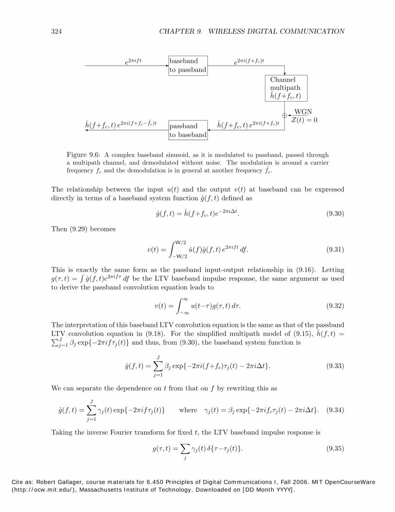
In transform terms, x(f) = u(f − fc) + u∗(−f + fc). The positive-frequency part of x(t) is simply u(t) shifted up by fc. To understand the modulation and demodulation in simplest terms,consider a baseband complex sinusoidal input e2πift for f ∈ [−W/2, W/2] as it is modulated,transmitted through the channel, and demodulated (see Figure 9.6). Since the channel maybe subject to Doppler shifts, the recovered carrier, fc, at the receiver might be different thanthe actual carrier fc. Thus, as illustrated, the positive-frequency channel output is yf (t) = h(f+fc, t) e2πi(f+fc)t and the demodulated waveform is h(f+fc, t) e2πi(f+fc−fc)t .
For an arbitrary baseband-limited input, u(t) = ∫ −WW/2 /2 u(f)e2πift df , the positive-frequency chan
nel output is given by superposition as∫ W/2
y +(t) = u(f)h(f+fc, t) e 2πi(f+fc)t df. −W/2
The demodulated waveform, v(t), is then y+(t) shifted down by the recovered carrier fc, i.e., ∫ W/2
v(t) = u(f)h(f+fc, t) e 2πi(f+fc−fc)t df. −W/2
Let ∆ be the difference between recovered and transmitted carrier,12 i.e., ∆ = fc − fc. Thus ∫ W/2
v(t) = u(f)h(f+fc, t) e 2πi(f−∆)t df. (9.29) −W/2
12It might be helpful to assume ∆ 0 on a first reading. =
Cite as: Robert Gallager, course materials for 6.450 Principles of Digital Communications I, Fall 2006. MIT OpenCourseWare (http://ocw.mit.edu/), Massachusetts Institute of Technology. Downloaded on [DD Month YYYY].
∫ ∫
∑
∑
∑
324 CHAPTER 9. WIRELESS DIGITAL COMMUNICATION
�e2πift baseband to passband
e2πi(f+fc)t
� Channel multipathh(f+fc, t)
WGN Z(t) = 0
h(f+fc, t) e2πi(f+fc)th(f+fc, t) e2πi(f+fc− fc)t � passband
to baseband �
⊕�
Figure 9.6: A complex baseband sinusoid, as it is modulated to passband, passed through a multipath channel, and demodulated without noise. The modulation is around a carrier frequency fc and the demodulation is in general at another frequency fc.
The relationship between the input u(t) and the output v(t) at baseband can be expressed directly in terms of a baseband system function g(f, t) defined as
g(f, t) = h(f+fc, t)e−2πi∆t . (9.30)
Then (9.29) becomes ∫ W/2
v(t) = u(f)g(f, t) e 2πift df. (9.31) −W/2
This is exactly the same form as the passband input-output relationship in (9.16). Letting g(τ, t) = g(f, t)e2πifτ df be the LTV baseband impulse response, the same argument as used to derive the passband convolution equation leads to
v(t) = ∞
u(t−τ)g(τ, t) dτ. (9.32) −∞
The interpretation of this baseband LTV convolution equation is the same as that of the passband LTV convolution equation in (9.18). For the simplified multipath model of (9.15), h(f, t) =∑J βj exp{−2πifτj(t)} and thus, from (9.30), the baseband system function is j=1
J
g(f, t) = βj exp{−2πi(f+fc)τj(t) − 2πi∆t}. (9.33) j=1
We can separate the dependence on t from that on f by rewriting this as
J
g(f, t) = γj(t) exp{−2πifτj(t)} where γj(t) = βj exp{−2πifcτj(t) − 2πi∆t}. (9.34) j=1
Taking the inverse Fourier transform for fixed t, the LTV baseband impulse response is
g(τ, t) = γj(t) δ{τ−τj(t)}. (9.35) j
Cite as: Robert Gallager, course materials for 6.450 Principles of Digital Communications I, Fall 2006. MIT OpenCourseWare (http://ocw.mit.edu/), Massachusetts Institute of Technology. Downloaded on [DD Month YYYY].
∑
∑
9.4. BASEBAND SYSTEM FUNCTIONS AND IMPULSE RESPONSES 325
Thus the impulse response at a given receive-time t is a sum of impulses, the jth of which is delayed by τj (t) and has an attenuation and phase given by γj (t). Substituting this impulse response into the convolution equation, the input-output relation is
v(t) = γj (t) u(t−τj (t)). j
This baseband representation can provide additional insight about Doppler spread and coherence time. Consider the system function in (9.34) at f = 0 (i.e., at the passband carrier frequency). Letting Dj be the Doppler shift at fc on path j, we have τj (t) = τj
o −Dj t/fc. Then
J
g(0, t) = γj (t) where γj (t) = βj exp{2πi[Dj − ∆]t − 2πifcτjo}.
j=1
The carrier recovery circuit estimates the carrier frequency from the received sum of Doppler shifted versions of the carrier, and thus it is reasonable to approximate the shift in the recovered carrier by the midpoint between the smallest and largest Doppler shift. Thus g(0, t) is the same as the frequency-shifted system function ψ(fc, t) of (9.24). In other words, the frequency shift ∆, which was introduced in (9.24) as a mathematical artifice, now has a physical interpretation as the difference between fc and the recovered carrier fc. We see that g(0, t) is a waveform with bandwidth D/2, and that Tcoh = 1/(2D) is an order-of-magnitude approximation to the time over which g(0, t) changes significantly.
Next consider the baseband system function g(f, t) at baseband frequencies other than 0. Since W � fc, the Doppler spread at fc + f is approximately equal to that at fc, and thus g(f, t), as a function of t for each f ≤ W/2, is also approximately baseband limited to D/2 (where D is defined at f = fc).
Finally, consider flat fading from a baseband perspective. Flat fading occurs when W � Fcoh, and in this case13 g(f, t) ≈ g(0, t). Then, from (9.31),
v(t) = g(0, t)u(t). (9.36)
In other words, the received waveform, in the absence of noise, is simply an attenuated and phase shifted version of the input waveform. If the carrier recovery circuit also recovers phase, then v(t) is simply an attenuated version of u(t). For flat fading, then, Tcoh is the order-of-magnitude interval over which the ratio of output to input can change significantly.
In summary, this section has provided both a passband and baseband model for wireless communication. The basic equations are very similar, but the baseband model is somewhat easier to use (although somewhat more removed from the physics of fading). The ease of use comes from the fact that all the waveforms are slowly varying and all are complex. This can be seen most clearly by comparing the flat-fading relations, (9.28) for passband and (9.36) for baseband.
9.4.1 A discrete-time baseband model
This section uses the sampling theorem to convert the above continuous-time baseband channel to a discrete-time channel. If the baseband input u(t) is bandlimited to W/2, then it can be
13There is an important difference between saying that the Doppler spread at frequency f+fc is close to that at fc and saying that g(f, t) ≈ g(0, t). The first requires only that W be a relatively small fraction of fc, and is reasonable even for W = 100 mH and fc = 1gH, whereas the second requires W � Fcoh, which might be on the order of hundreds of kH.
Cite as: Robert Gallager, course materials for 6.450 Principles of Digital Communications I, Fall 2006. MIT OpenCourseWare (http://ocw.mit.edu/), Massachusetts Institute of Technology. Downloaded on [DD Month YYYY].
∑ ∑
∫
∑
∫ ∑ ∫
∑
∑ [ ]
326 CHAPTER 9. WIRELESS DIGITAL COMMUNICATION
represented by its T -spaced samples, T = 1/W, as u(t) = usinc( t − ), where u = u( T ).T Using (9.32), the baseband output is given by
v(t) = u g(τ, t) sinc(t/T − τ/T − ) dτ. (9.37)
The sampled outputs, vm = v(mT ), at multiples of T are then given by14
vm = u g(τ, mT ) sinc(m − − τ/T ) dτ (9.38)
= um−k g(τ, mT ) sinc(k − τ/T ) dτ, . (9.39) k
where k = m− . By labeling the above integral as gk,m, (9.39) can be written in the discrete-time form ∑ ∫
vm = gk,m um−k where gk,m = g(τ, mT ) sinc(k − τ/T ) dτ. (9.40) k
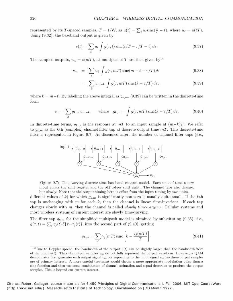
In discrete-time terms, gk,m is the response at mT to an input sample at (m−k)T . We refer to gk,m as the kth (complex) channel filter tap at discrete output time mT . This discrete-time filter is represented in Figure 9.7. As discussed later, the number of channel filter taps (i.e.,
input um+2 um+1 um um−1 um−2
���� ���� ���� ���� �� � � � ��g1,m g2,mg−1,m g0,mg−2,m
� � � � �
� � vm
Figure 9.7: Time-varying discrete-time baseband channel model. Each unit of time a new input enters the shift register and the old values shift right. The channel taps also change, but slowly. Note that the output timing here is offset from the input timing by two units.
different values of k) for which gk,m is significantly non-zero is usually quite small. If the kth tap is unchanging with m for each k, then the channel is linear time-invariant. If each tap changes slowly with m, then the channel is called slowly time-varying. Cellular systems and most wireless systems of current interest are slowly time-varying.
The filter tap gk,m for the simplified multipath model is obtained by substituting (9.35), i.e., g(τ, t) = γj(t) δ{τ−τj(t)}, into the second part of (9.40), gettingj
gk,m = ∑
γj(mT ) sinc k − τj(mT )
. (9.41)T
j
14Due to Doppler spread, the bandwidth of the output v(t) can be slightly larger than the bandwidth W/2 of the input u(t). Thus the output samples vm do not fully represent the output waveform. However, a QAM demodulator first generates each output signal vm corresponding to the input signal um, so these output samples are of primary interest. A more careful treatment would choose a more appropriate modulation pulse than a sinc function and then use some combination of channel estimation and signal detection to produce the output samples. This is beyond our current interest.
Cite as: Robert Gallager, course materials for 6.450 Principles of Digital Communications I, Fall 2006. MIT OpenCourseWare (http://ocw.mit.edu/), Massachusetts Institute of Technology. Downloaded on [DD Month YYYY].
9.4. BASEBAND SYSTEM FUNCTIONS AND IMPULSE RESPONSES 327
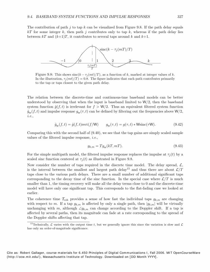
The contribution of path j to tap k can be visualized from Figure 9.8. If the path delay equals kT for some integer k, then path j contributes only to tap k, whereas if the path delay lies between kT and (k+1)T , it contributes to several taps around k and k+1.
sinc(k − τj(mT )/T )
0 1 2 3 k−1 τj (mT )
T
Figure 9.8: This shows sinc(k − τj (mt)/T ), as a function of k, marked at integer values of k. In the illustration, τj (mt)/T ) = 0.8. The figure indicates that each path contributes primarily to the tap or taps closest to the given path delay.
The relation between the discrete-time and continuous-tme baseband models can be better understood by observing that when the input is baseband limited to W/2, then the baseband system function g(f, t) is irrelevant for f > W/2. Thus an equivalent filtered system function g (f, t) and impulse response g (τ, t) can be defined by filtering out the frequencies above W/2,
W W
i.e.,
gW(f, t) = g(f, t)rect(f/W) g
W(τ, t) = g(τ, t) ∗ Wsinc(τW). (9.42)
Comparing this with the second half of (9.40), we see that the tap gains are simply scaled sample values of the filtered impulse response, i.e.,
gk,m = TgW(kT,mT ). (9.43)
For the simple multipath model, the filtered impulse response replaces the impulse at τj(t) by a scaled sinc function centered at τj(t) as illustrated in Figure 9.8.
Now consider the number of taps required in the discrete time model. The delay spread, L, is the interval between the smallest and largest path delay15 and thus there are about L/T taps close to the various path delays. There are a small number of additional significant taps corresponding to the decay time of the sinc function. In the special case where L/T is much smaller than 1, the timing recovery will make all the delay terms close to 0 and the discrete-time model will have only one significant tap. This corresponds to the flat-fading case we looked at earlier.
The coherence time Tcoh provides a sense of how fast the individual taps gk,m are changing with respect to m. If a tap gk,m is affected by only a single path, then |gk,m| will be virtually unchanging with m, although ∠gk,m can change according to the Doppler shift. If a tap is affected by several paths, then its magnitude can fade at a rate corresponding to the spread of the Doppler shifts affecting that tap.
15Technically, L varies with the output time t, but we generally ignore this since the variation is slow and Lhas only an order-of-magnitude significance.
Cite as: Robert Gallager, course materials for 6.450 Principles of Digital Communications I, Fall 2006. MIT OpenCourseWare (http://ocw.mit.edu/), Massachusetts Institute of Technology. Downloaded on [DD Month YYYY].

{ }
{ }
328 CHAPTER 9. WIRELESS DIGITAL COMMUNICATION
9.5 Statistical channel models
The previous subsection created a discrete-time baseband fading channel in which the individual tap gains gk,m in (9.41) are scaled sums of the attenuation and smoothed delay on each path. The physical paths are unknown at the transmitter and receiver, however, so from an input/output viewpoint, it is the tap gains themselves16 that are of primary interest. Since these tap gains change with time, location, bandwidth, carrier frequency, and other parameters, a statistical characterization of the tap gains is needed in order to understand how to communicate over these channels. This means that each tap gain gk,m should be viewed as a sample value of a random variable Gk,m.
There are many approaches to characterizing these tap-gain random variables. One would be to gather statistics over a very large number of locations and conditions, and then model the joint probability densities of these random variables according to these measurements, and do this conditionally on various types of locations (cities, hilly areas, flat areas, highways, buildings, etc.). Much data of this type has been gathered, but it is more detailed than what is desirable to achieve an initial understanding of wireless issues.
Another approach, which is taken here and in virtually all the theoretical work in the field, is to choose a few very simple probability models that are easy to work with, and then use the results from these models to gain insight about actual physical situations. After presenting the models, we discuss the ways in which the models might or might not reflect physical reality. Some standard results are then derived from these models, along with a discussion of how they might reflect actual performance.
In the Rayleigh tap-gain model, the real and imaginary parts of all the tap gains are taken to be zero-mean jointly-Gaussian random variables. Each tap gain Gk,m is thus a complex Gaussian random variable which is further assumed to be circularly symmetric, i.e., to have iid real and imaginary parts. Finally it is assumed that the probability density of each Gk,m is the same for all m. We can then express the probability density of Gk,m as
1 2 2
f�(Gk,m),�(Gk,m)(gre, gim) =2πσ2 exp
−gre
2σ
−2
gim , (9.44) k k
where σ2 is the variance of �(Gk,m) (and thus also of �(Gk,m)) for each m. We later address k how these rv’s are related between different m and k.
As shown in Exercise 7.1, the magnitude |Gk,m| of the kth tap is a Rayleigh rv with density
2
f ( g ) = |g|
exp −|g|
. (9.45)|Gk,m| | |σk
2 2σk 2
This model is called the Rayleigh fading model. Note from (9.44) that the model includes a uniformly distributed phase that is independent of the Rayleigh distributed amplitude. The assumption of uniform phase is quite reasonable, even in a situation with only a small number of paths, since a quarter wavelength at cellular frequencies is only a few inches. Thus even with fairly accurately specified path lengths, we would expect the phases to be modeled as uniform
16Many wireless channels are characterized by a very small number of significant paths, and the corresponding receivers track these individual paths rather than using a receiver structure based on the discrete-time model. The discrete-time model is none-the-less a useful conceptual model for understanding the statistical variation of multiple paths.
Cite as: Robert Gallager, course materials for 6.450 Principles of Digital Communications I, Fall 2006. MIT OpenCourseWare (http://ocw.mit.edu/), Massachusetts Institute of Technology. Downloaded on [DD Month YYYY].
9.5. STATISTICAL CHANNEL MODELS 329
and independent of each other. This would also make the assumption of independence between tap-gain phase and amplitude reasonable.
The assumption of Rayleigh distributed amplitudes is more problematic. If the channel involves scattering from a large number of small reflectors, the central limit theorem would suggest a jointly Gaussian assumption for the tap gains,17 thus making (9.44) reasonable. For situations with a small number of paths, however, there is no good justification for (9.44) or (9.45).
There is a frequently used alternative model in which the line of sight path (often called a specular path) has a known large magnitude, and is accompanied by a large number of independent smaller paths. In this case, gk,m, at least for one value of k, can be modeled as a sample value of a complex Gaussian rv with a mean (corresponding to the specular path) plus real and imaginary iid fluctuations around the mean. The magnitude of such a rv has a Rician distribution. Its density has quite a complicated form, but the error probability for simple signaling over this channel model is quite simple and instructive.
The preceding paragraphs make it appear as if a model is being constructed for some known number of paths of given character. Much of the reason for wanting a statistical model, however, is to guide the design of transmitters and receivers. Having a large number of models means investigating the performance of given schemes over all such models, or measuring the channel, choosing an appropriate model, and switching to a scheme appropriate for that model. This is inappropriate for an initial treatment, and perhaps inappropriate for design, returning us to the Rayleigh and Rician models. One reasonable point of view here is that these models are often poor approximations for individual physical situations, but when averaged over all the physical situations that a wireless system must operate over, they make more sense.18 At any rate, these models provide a number of insights into communication in the presence of fading.
Modeling each gk,m as a sample value of a complex rv Gk,m provides part of the needed statistical description, but this is not the only issue. The other major issue is how these quantities vary with time. In the Rayleigh fading model, these random variables have zero mean, and it will make a great deal of difference to useful communication techniques if the sample values can be estimated in terms of previous values. A statistical quantity that models this relationship is known as the tap-gain correlation function, R(k, ∆). It is defined as
R(k, n) = E[Gk,mG∗ ]. (9.46)k,m+∆
This gives the autocorrelation function of the sequence of complex random variables, modeling each given tap k as it evolves in time. It is tacitly assumed that this is not a function of time m, which means that the sequence {Gk,m; m ∈ Z} for each k is assumed to be wide-sense stationary. It is also assumed that, as a random variable, Gk,m is independent of Gk′,m′ for all k =� k′ and all m, m′. This final assumption is intuitively plausible19 since paths in different ranges of delay contribute to Gk,m for different values of k.
The tap-gain correlation function is useful as a way of expressing the statistics for how tap gains change, given a particular bandwidth W. It does not address the questions comparing different
17In fact, much of the current theory of fading was built up in the 1960s when both space communication and military channels of interest then were well modeled as scattering channels with a very large number of small reflectors.
18This is somewhat oversimplified. As shown in Exercise 9.9, a random choice of a small number of paths from a large possible set does not necessarily lead to a Rayleigh distribution. There is also the question of an initial choice of power level at any given location.
19One could argue that a moving path would gradually travel from the range of one tap to another. This is true, but the time intervals for such changes are typically large relative to the other intervals of interest.
Cite as: Robert Gallager, course materials for 6.450 Principles of Digital Communications I, Fall 2006. MIT OpenCourseWare (http://ocw.mit.edu/), Massachusetts Institute of Technology. Downloaded on [DD Month YYYY].
∑ ∑
| | ∑ ∑
330 CHAPTER 9. WIRELESS DIGITAL COMMUNICATION
bandwidths for communication. If we visualize increasing the bandwidth, several things happen. First, since the taps are separated in time by 1/W, the range of delay corresponding to a single tap becomes narrower. Thus there are fewer paths contributing to each tap, and the Rayleigh approximation can in many cases become poorer. Second, the sinc functions of (9.41) become narrower, so the path delays spill over less in time. For this same reason, R(k, 0) for each k gives a finer grained picture of the amount of power being received in the delay window of width k/W. In summary, as this model is applied to larger W, more detailed statistical information is provided about delay and correlation at that delay, but the information becomes more questionable.
In terms of R(k, ∆), the multipath spread L might be defined as the range of kT over which R(k, 0) is significantly non-zero. This is somewhat preferable to the previous “definition” in that the statistical nature of L becomes explicit and the reliance on some sort of stationarity becomes explicit. In order for this definition to make much sense, however, the bandwidth W must be large enough for several significant taps to exist.
The coherence time Tcoh can also be defined more explicitly as mT for the smallest value of ∆ > 0 for which R(0, ∆) is significantly different from R(0, 0). Both these definitions maintain some ambiguity about what ‘significant’ means, but they face the reality that L and Tcoh should be viewed probabilistically rather than as instantaneous values.
9.5.1 Passband and baseband noise
The statistical channel model above focuses on how multiple paths and Doppler shifts can affect the relationship between input and output, but the noise and the interference from other wireless channels have been ignored. The interference from other users will continue to be ignored (except for regarding it as additional noise), but the noise will now be included.
Assume that the noise is WGN with power WN0 over the bandwidth W. The earlier convention will still be followed of measuring both signal power and noise power at baseband. Extending the deterministic baseband input/output model vm = k gk,mum−k to include noise as well as randomly varying gap gains,
Vm = Gk,mUm−k + Zm, (9.47) k
where . . . , Z−1, Z0, Z1, . . . , is a sequence of iid circularly symmetric complex Gaussian random variables. Assume also that the inputs, the tap gains, and the noise are statistically independent of each other.
The assumption of WGN essentially means that the primary source of noise is at the receiver or is radiation impinging on the receiver that is independent of the paths over which the signal is being received. This is normally a very good assumption for most communication situations. Since the inputs and outputs here have been modeled as samples at rate W of the baseband processes, we have E[|Um|2] = P where P is the baseband input power constraint. Similarly, E[ Zm
2] = N0W. Each complex noise rv is thus denoted as Zm ∼ CN (0, WN0)
The channel tap gains will be normalized so that Vm′ = k Gk,mUm−k satisfies E[|Vm
′ |2] = P . It can be seen that this normalization is achieved by
E[ |Gk,0|2] = 1. (9.48) k
Cite as: Robert Gallager, course materials for 6.450 Principles of Digital Communications I, Fall 2006. MIT OpenCourseWare (http://ocw.mit.edu/), Massachusetts Institute of Technology. Downloaded on [DD Month YYYY].
9.6. DATA DETECTION 331
This assumption is similar to our earlier assumption for the ordinary (non-fading) WGN channel that the overall attenuation of the channel is removed from consideration. In other words, both here and there we are defining signal power as the power of the received signal in the absence of noise. This is conventional in the communication field and allows us to separate the issue of attenuation from that of coding and modulation.
It is important to recognize that this assumption cannot be used in a system where feedback from receiver to transmitter is used to alter the signal power when the channel is faded.
There has always been a certain amount of awkwardness about scaling from baseband to passband, where the signal power and noise power each increase by a factor of 2. Note that we have also gone from a passband channel filter H(f, t) to a baseband filter G(f, t) using the same convention as used for input and output. It is not difficult to show that if this property of treating signals and channel filters identically is preserved, and the convolution equation is preserved at baseband and passband, then losing a factor of 2 in power is inevitable in going from passband to baseband.
9.6 Data detection
A reasonable approach to detection for wireless channels is to measure the channel filter taps as they evolve in time, and to use these measured values in detecting data. If the response can be measured accurately, then the detection problem becomes very similar to that for wireline channels; i.e., detection in WGN.
Even under these ideal conditions, however, there are a number of problems. For one thing, even if the transmitter has perfect feedback about the state of the channel, power control is a difficult question; namely, how much power should be sent as a function of the channel state?
For voice, both maintaining voice quality and maintaining small constant delay is important. This leads to a desire to send information at a constant rate, which in turn leads to increased transmission power when the channel is poor. This is very wasteful of power, however, since common sense says that if power is scarce and delay is unimportant, then the power and transmission rate should be decreased when the channel is poor.
Increasing power when the channel is poor has a mixed impact on interference between users. This strategy maintains equal received power at a base station for all users in the cell corresponding to that base station. This helps reduce the effect of multiaccess interference within the same cell. The interference between neighboring cells can be particularly bad, however, since fading on the channel between a cell phone and its base station is not highly correlated with fading between that cell phone and another base station.
For data, delay is less important, so data can be sent at high rate when the channel is good, and at low rate (or zero rate) when the channel is poor. There is a straightforward information-theoretic technique called water filling that can be used to maximize overall transmission rate at a given overall power. The scaling assumption that we made above about input and output power must be modified for all of these issues of power control.
An important insight from this discussion is that the power control used for voice should be very different from that for data. If the same system is used for both voice and data applications, then the basic mechanisms for controlling power and rate should be very different for the two applications.
Cite as: Robert Gallager, course materials for 6.450 Principles of Digital Communications I, Fall 2006. MIT OpenCourseWare (http://ocw.mit.edu/), Massachusetts Institute of Technology. Downloaded on [DD Month YYYY].
332 CHAPTER 9. WIRELESS DIGITAL COMMUNICATION
In this section, power control and rate control are not considered, and the focus is simply on detecting signals under various assumptions about the channel and the state of knowledge at the receiver.
9.6.1 Binary detection in flat Rayleigh fading
Consider a very simple example of communication in the absence of channel measurement. Assume that the channel can be represented by a single discrete-time complex filter tap G0,m, which we abbreviate as Gm. Also assume Rayleigh fading; i.e., the probability density of the magnitude of each Gm is
f|Gm|(|g|) = 2|g| exp{−|g|2} ; |g| ≥ 0, (9.49)
or, equivalently, the density of γ = |Gm|2 ≥ 0 is
f(γ) = exp(−γ) ; γ ≥ 0. (9.50)
The phase is uniform over [0, 2π) and independent of the magnitude. Equivalently, the real and imaginary parts of Gm are iid Gaussian, each with variance 1/2. The Rayleigh fading has been scaled in this way to maintain equality between the input power, E[ 2], and the output signal
2 |Um|
power, E[|Um| |Gm|2]. It is assumed that Um and Gm are independent, i.e., that feedback is not used to control the input power as a function of the fading. For the time being, however, the dependence between the taps Gm at different times m is not relevant.
This model is called flat fading for the following reason. A single-tap discrete-time model, where v(mT ) = g0,mu(mT ), corresponds to a continuous-time baseband model for which g(τ, t) = g(0, t)sinc(τ/T ). Thus the baseband system function for the channel is given by g(f, t) = g0(t)rect(fT ). Thus the fading is constant (i.e., flat) over the baseband frequency range used for communication. When more than one tap is required, the fading varies over the baseband region. To state this another way, the flat fading model is appropriate when the coherence frequency is greater than the baseband bandwidth.
Consider using binary antipodal signaling with Um = ±a for each m. Assume that {Um; m ∈ Z}is an iid sequence with equiprobable use of plus and minus a. This signaling scheme fails completely, even in the absence of noise, since the phase of the received symbol is uniformly distributed between 0 and 2π under each hypothesis, and the received amplitude is similarly independent of the hypothesis. It is easy to see that phase modulation is similarly flawed. In fact, signal structures must be used in which either different symbols have different magnitudes, or, alternatively, successive signals must be dependent.20
Next consider a form of binary pulse-position modulation where, for each pair of time-samples, one of two possible signal pairs, (a, 0) or (0, a), is sent. (This has the same performance as a number of binary orthogonal modulation schemes such as minimum shift keying (see Exercise 8.16)), but is simpler to describe in discrete time. The output is then
Vm = UmGm + Zm, m = 0, 1, (9.51)
where, under one hypothesis, the input signal pair is U = (a, 0), and under the other hypothesis, U = (0, a). The noise samples, {Zm; m ∈ Z} are iid circularly symmetric complex Gaussian
20For example, if the channel is slowly varying, differential phase modulation, where data is sent by the difference between the phase of successive signals, could be used.
Cite as: Robert Gallager, course materials for 6.450 Principles of Digital Communications I, Fall 2006. MIT OpenCourseWare (http://ocw.mit.edu/), Massachusetts Institute of Technology. Downloaded on [DD Month YYYY].
{ }
{ }
{ } [ ]
{ } { }
∫ { }
9.6. DATA DETECTION 333
random variables, Zm ∼ CN (0, N0W ). Assume for now that the detector looks only at the outputs V0 and V1.
Given U = (a, 0), V0 = aG0 + Z0 is the sum of two independent complex Gaussian random variables, the first with variance a2/2 per dimension, and the second with variance N0W/2 per dimension. Thus, given U = (a, 0), the real and imaginary parts of V0 are independent, each N (0, a2/2 + N0W/2). Similarly, given U = (a, 0), the real and imaginary parts of V1 = Z1
are independent, each N (0, N0W/2). Finally, since the noise variables are independent, V0 and V1 are independent (given U = (a, 0)). The joint probability density21 of (V0, V1) at (v0, v1), conditional on hypothesis U = (a, 0), is therefore
f0(v0, v1) = 1
exp |v0|2 |v1|2
. (9.52)(2π)2(a2/2 + WN0/2)(WN0/2)
− a2 + WN0
− WN0
where f0 denotes the conditional density given hypothesis U=(a, 0). Note that the density in (9.52) depends only on the magnitude and not the phase of v0 and v1. Treating the alternate hypothesis in the same way, and letting f1 denote the conditional density given U = (0, a),
f1(v0, v1) = 1
exp |v0|2 |v1|2
. (9.53)(2π)2(a2/2 + WN0/2)(WN0/2)
− WN0
− a2 + WN0
The log likelihood ratio is then
LLR(v0, v1) = ln f0(v0, v1) =
|v0|2 − |v1|2 a2
. (9.54)f1(v0, v1) (a2 + WN0)(WN0)
2The maximum likelihood (ML) decision rule is therefore to decode U=(a, 0) if |v0| ≥ |v1|2 and decode U=(0, a) otherwise. Given the symmetry of the problem, this is certainly no surprise. It may however be somewhat surprising that this rule does not depend on any possible dependence between G0 and G1.
Next consider the ML probability of error. Let Xm = |Vm|2 for m = 0, 1. The probability densities of X0 ≥ 0 and X1 ≥ 0, conditioning on U = (a, 0) throughout, are then given by
1 x0 1 x1fX0
(x0) = a2+WN0
exp −a2+WN0
; fX1 (x1) =
WN0 exp −
WN0 .
xThen, Pr(X1 > x) = exp(− ) for x ≥ 0, and therefore WN0
∞ 1 x0 x0Pr(X1 > X0) = a2+WN0
exp −a2+WN0
exp{−WN0
} dx0 0
1 = 2 . (9.55)
2 + aWN0
Since X1 > X0 is the condition for an error when U = (a, 0), this is Pr(e) under the hypothesis U = (a, 0). By symmetry, the error probability is the same under the hypothesis U = (0, a), so this is the unconditional probability of error.
21V0 and V1 are complex random variables, so the probability density of each is defined as probability per unit area in the real and complex plane. If V0 and V1 are represented by amplitude and phase, for example, the densities are different.
Cite as: Robert Gallager, course materials for 6.450 Principles of Digital Communications I, Fall 2006. MIT OpenCourseWare (http://ocw.mit.edu/), Massachusetts Institute of Technology. Downloaded on [DD Month YYYY].
334 CHAPTER 9. WIRELESS DIGITAL COMMUNICATION
The mean signal power is a2/2 since half the inputs have a square value a2 and half have value 0. There are W/2 binary symbols per second, so Eb, the energy per bit, is a2/W. Substituting this into (9.55),
1Pr(e) = . (9.56)
2 + Eb/N0
This is a very discouraging result. To get an error probability Pr(e) = 10−3 would require Eb/N0 ≈ 1000 (30 dB). Stupendous amounts of power would be required for more reliable communication.
After some reflection, however, this result is not too surprising. There is a constant signal energy Eb per bit, independent of the channel response Gm. The errors generally occur when the sample values |gm|2 are small; i.e., during fades. Thus the damage here is caused by the combination of fading and constant signal power. This result, and the result to follow, make it clear that to achieve reliable communication, it is necessary either to have diversity and/or coding between faded and unfaded parts of the channel, or to use channel measurement and feedback to control the signal power in the presence of fades.
9.6.2 Non-coherent detection with known channel magnitude
Consider the same binary pulse position modulation of the previous subsection, but now assume that G0 and G1 have the same magnitude, and that the sample value of this magnitude, say g, is a fixed parameter that is known at the receiver. The phase φm of Gm, m = 0, 1 is uniformly distributed over [0, 2π) and is unknown at the receiver. The term non-coherent detection is used for detection that does not make use of a recovered carrier phase, and thus applies here. We will see that the joint density of φ0 and φ1 is immaterial. Assume the same noise distribution as before. Under hypothesis U=(a, 0), the outputs V0 and V1 are given by
V0 = ag exp{iφ0} + Z0 ; V1 = Z1 (under U=(a, 0)). (9.57)
Similarly, under U=(0, a),
V0 = Z0 ; V1 = ag exp{iφ1} + Z1 (under U=(0, a)). (9.58)
Only V0 and V1, along with the fixed channel magnitude g, can be used in the decision, but it will turn out that the value of g is not needed for an ML decision. The channel phases φ0 and φ1 are not observed and cannot be used in the decision.
The probability density of a complex random variable is usually expressed as the joint density of the real and imaginary parts, but here it is more convenient to use the joint density of magnitude and phase. Since the phase φ0 of ag exp{iφ0} is uniformly distributed, and since Z0
is independent with uniform phase, it follows that V0 has uniform phase; i.e., ∠V0 is uniform conditional on U=(a, 0). The magnitude |V0|, conditional on U=(a, 0), is a Rician random variable which is independent of φ0, and therefore also independent of ∠V0. Thus, conditional on U=(a, 0), V0 has independent phase and amplitude, and uniformly distributed phase.
Similarly, conditional on U = (0, a), V0 = Z0 has independent phase and amplitude, and uniformly distributed phase. What this means is that both the hypothesis and |V0| are statistically independent of the phase ∠V0. It can be seen that they are also statistically independent of φ0.
Cite as: Robert Gallager, course materials for 6.450 Principles of Digital Communications I, Fall 2006. MIT OpenCourseWare (http://ocw.mit.edu/), Massachusetts Institute of Technology. Downloaded on [DD Month YYYY].
( )
( )
9.6. DATA DETECTION 335
Using the same argument on V1, we see that both the hypothesis and |V1| are statistically independent of the phases ∠V1 and φ1. It should then be clear that |V0|, |V1|, and the hypothesis are independent of the phases (∠V0, ∠V1, φ0, φ1). This means that the sample values |v0|2 and |v1|2 are sufficient statistics for choosing between the hypotheses U=(a, 0) and U=(0, a).
Given the sufficient statistics |v0|2 and |v1|2, we must determine the ML detection rule, again assuming equiprobable hypotheses. Since v0 contains the signal under hypothesis U=(a, 0), and v1 contains the signal under hypothesis U = (0, a), and since the problem is symmetric between U=(a, 0) and U = (0, a), it appears obvious that the ML detection rule is to choose U=(a, 0) if |v0|2 > |v1|2 and to choose U = (0, a) otherwise. Unfortunately, to show this analytically, it seems necessary to calculate the likelihood ratio. The appendix gives this likelihood ratio and calculates the probability of error. The error probability for a given g is derived there as
Pr(e) = 21
exp −2a
W
2g
N
2
0 . (9.59)
The mean received baseband signal power is a2g2/2 since only half the inputs are used. There are W/2 bits per second, so Eb = a2g2/W. Thus, this probability of error can be expressed as
Pr(e) = 1
exp −2E
Nb
0 (non − coherent). (9.60)
2
It is interesting to compare the performance of this non-coherent detector with that of a coherent detector (i.e., a detector such as those in Chapter 8 that use the carrier phase) for equal-energy orthogonal signals. As seen before, the error probability in the latter case is (√ ) √ ( )
Eb N0 EbPr(e) = QN0
≈ 2πEb
exp −2N0
(coherent). (9.61)
Thus both expressions have the same exponential decay with Eb/N0 and differ only in the coefficient. The error probability with non-coherent detection is still substantially higher22 than with coherent detection, but the difference is nothing like that in (9.56). More to the point, if Eb/N0 is large, we see that the additional energy per bit required in non-coherent communication to make the error probability equal to that of coherent communication is very small. In other words, a small increment in dB corresponds to a large decrease in error probability. Of course, with non-coherent detection, we also pay a 3 dB penalty for not being able to use antipodal signaling.
Early telephone-line modems (in the 1200 bits per second range) used non-coherent detection, but current high-speed wireline modems generally track the carrier phase and use coherent detection. Wireless systems are subject to rapid phase changes because of the transmission medium, so non-coherent techniques are still common there.
It is even more interesting to compare the non-coherent result here with the Rayleigh fading result. Note that both use the same detection rule, and thus knowledge of the magnitude of the channel strength at the receiver in the Rayleigh case would not reduce the error probability. As shown in Exercise 9.11, if we regard g as a sample value of a random variable that is known at
22As an example, achieving Pr(e) = 10−6 with non-coherent detection requires Eb/N0 to be 26.24, which would yield Pr(e) = 1.6 × 10⁻⁷ with coherent detection. However, it would require only about half a dB of additional power to achieve that lower error probability with non-coherent detection.
Cite as: Robert Gallager, course materials for 6.450 Principles of Digital Communications I, Fall 2006. MIT OpenCourseWare (http://ocw.mit.edu/), Massachusetts Institute of Technology. Downloaded on [DD Month YYYY].
336 CHAPTER 9. WIRELESS DIGITAL COMMUNICATION
the receiver, and average over the result in (9.59), then the error probability is the same as that in (9.56).
The conclusion from this comparison is that the real problem with binary communication over flat Rayleigh fading is that when the signal is badly faded, there is little hope for successful transmission using a fixed amount of signal energy. It has just been seen that knowledge of the fading amplitude at the receiver does not help. Also, as seen in the second part of Exercise 9.11, using power control at the transmitter to maintain a fixed error probability for binary communication leads to infinite average transmission power. The only hope, then, is either to use variable rate transmission or to use coding and/or diversity. In this latter case, knowledge of the fading magnitude will be helpful at the receiver in knowing how to weight different outputs in making a block decision.
Finally, consider the use of only V0 and V1 in binary detection for Rayleigh fading and non-coherent detection. If there are no inputs other than the binary input at times 0 and 1, then all other outputs can be seen to be independent of the hypothesis and of V0 and V1. If there are other inputs, however, the resulting outputs can be used to measure both the phase and amplitude of the channel taps.
The results in the previous two sections apply to any pair of equal energy baseband signals that are orthogonal as complex waveforms (i.e., the real and imaginary parts of one waveform are orthogonal to both the real and imaginary parts of the other waveform). For this more general result, however, we must assume that Gm is constant over the range of m used by the signals.
9.6.3 Non-coherent detection in flat Rician fading
Flat Rician fading occurs when the channel can be represented by a single tap and one path is significantly stronger than the other paths. This is a reasonable model when a line of sight path exists between transmitter and receiver, accompanied by various reflected paths. Perhaps more important, this model provides a convenient middle ground between a large number of weak paths, modeled by Rayleigh fading, and a single path with random phase, modeled in the last subsection. The error probability is easy to calculate in the Rician case, and contains the Rayleigh case and known magnitude case as special cases. When we study diversity, the Rician model provides additional insight into the benefits of diversity.
As with Rayleigh fading, consider binary pulse position modulation where U = u0 = (a, 0) under one hypothesis and U = u1 = (0, a) under the other hypothesis. The corresponding outputs are then
V0 = U0G0 + Z0 and V1 = U1G1 + Z1.
Using non-coherent detection, ML detection is the same for Rayleigh, Rician, or deterministic channels, i.e., given sample values v0 and v1 at the receiver,
U=u0
2 2 v0≥
v1 (9.62)| |<
| |U=u1
The magnitude of the strong path is denoted by g and the collective variance of the weaker paths is denoted by σg
2. Since only the magnitude of v0 and v1 are used in detection, the phase
Cite as: Robert Gallager, course materials for 6.450 Principles of Digital Communications I, Fall 2006. MIT OpenCourseWare (http://ocw.mit.edu/), Massachusetts Institute of Technology. Downloaded on [DD Month YYYY].
[ ]
[ ]
9.6. DATA DETECTION 337
of the tap gains G0 and G1 do not affect the decision, so the tap gains can be modeled as G0 ∼ G1 ∼ CN (g, σg
2). This is explained more fully, for the known magnitude case, in the appendix.
From the symmetry between the two hypotheses, the error probability is clearly the same for both. Thus the error probability will be calculated conditional on U = u0. All of the following probabilities and probability densities are assumed to be conditional on U = u0 . Under this conditioning, the real and imaginary parts of V0 and V1 are independent and characterized by
V0,re ∼ N (ag, σ02) V0,im ∼ N (0, σ0
2) V1,re ∼ N (0, σ1
2) V1,im ∼ N (0, σ12),
where
WN0 + a2σ2 WN0σ2 = g
σ2 = (9.63)0 12 2
Observe that |V1|2 is an exponentially distributed rv and for any x ≥ 0, Pr(|V1|2 ≥ x) = exp(−x/2σ1
2). Thus the probability of error, conditional on |V0|2 = x, is exp(−x/2σ12). The
unconditional probability of error (still conditioning on U = u0) can then be found by averaging over V 0.
Pr(e) = ∫ ∞ ∫ ∞ 1
exp
[ (v0,re − ag)2 v0
2 ,im
] exp
[ v0
2 ,re + v0
2 ,im
] dv0,re dv0.im2πσ0
2 − 2σ0
2 − 2σ0
2 − 2σ1
2 −∞ −∞
Integrating this over v0,im,
Pr(e) =
√ 2πσ0
2σ12 ∫ ∞ 1
exp
[ (v0,re − ag)2 v0
2 ,re
] σ2 + σ2 2πσ2 −
2σ2 − 2σ2 dv0,re
0 1 −∞ 0 0 1
This can be integrated by completing the square in the exponent, resulting in
σ2 a2g2 1
σ01 + σ1
2 exp −2(σ0
2 + σ12)
Substituting the values for σ0 and σ1 from (9.63), the result is
Pr(e) = 1
2σg 2 exp −
2WN
g
0
2a
+
2
a2σ22 + a g
WN0
Finally, the channel gain should be normalized so that g2 + σg 2 = 1. Then Eb becomes a2/W
and
1 g2EbPr(e) = exp (9.64) g 2N0 + Ebσ2
2 + Ebσ2 − g
N0
In the Rayleigh fading case, g = 0 and σg 2 = 1, simplifying Pr(e) to 2+E
1 b/N0
agreeing with the result derived earlier. For the fixed amplitude case, g = 1 and σg
2 = 0, reducing Pr(e) to 1 exp(−Eb/2N0), again agreeing with the earlier result. 2
Cite as: Robert Gallager, course materials for 6.450 Principles of Digital Communications I, Fall 2006. MIT OpenCourseWare (http://ocw.mit.edu/), Massachusetts Institute of Technology. Downloaded on [DD Month YYYY].
338 CHAPTER 9. WIRELESS DIGITAL COMMUNICATION
It is important to realize that this result does not depend on the receiver knowing that a strong path exists, since the detection rule is the same for non-coherent detection whether the fading is Rayleigh, Rician, or deterministic. The result says that with Rician fading, the error probability can be much smaller than with Rayleigh. However, if σg
2 > 0, the exponent approaches a constant with increasing Eb, and Pr(e) still goes to zero with (Eb/N0)−1. What this says, then, is that this slow approach to zero error probability with increasing Eb can not be avoided by a strong specular path, but only by the lack of an arbitrarily large number of arbitrarily weak paths. This is discussed further when we discuss diversity.
9.7 Channel measurement
This section introduces the topic of dynamically measuring the taps in the discrete-time baseband model of a wireless channel. Such measurements are made at the receiver based on the received waveform. They can be used to improve the detection of the received data, and, by sending the measurements back to the transmitter, to help in power and rate control at the transmitter.
One approach to channel measurement is to allocate a certain portion of each transmitted packet for that purpose. During this period, a known probing sequence is transmitted and the receiver uses this known sequence either to estimate the current values for the taps in the discrete-time baseband model of the channel or to measure the actual paths in a continuous-time baseband model. Assuming that the actual values for these taps or paths do not change rapidly, these estimated values can then help in detecting the remainder of the packet.
Another technique for channel measurement is called a rake receiver. Here the detection of the data and the estimation of the channel are done together. For each received data symbol, the symbol is detected using the previous estimate of the channel and then the channel estimate is updated for use on the next data symbol.
Before studying these measurement techniques, it will be helpful to understand how such measurements will help in detection. In studying binary detection for flat-fading Rayleigh channels, we saw that the error probability is very high in periods of deep fading, and that these periods are frequent enough to make the overall error probability large even when Eb/N0 is large. In studying non-coherent detection, we found that the ML detector does not use its knowledge of the channel strength, and thus, for binary detection in flat Rayleigh fading, knowledge at the receiver of the channel strength is not helpful. Finally, we saw that when the channel is good (the instantaneous Eb/N0 is high), knowing the phase at the receiver is of only limited benefit.
It turns out, however, that binary detection on a flat-fading channel is very much a special case, and that channel measurement can be very helpful at the receiver both for non-flat fading and for larger signal sets such as coded systems. Essentially, when the receiver observation consists of many degrees of freedom, knowledge of the channel helps the detector weight these degrees of freedom appropriately.
Feeding channel measurement information back to the transmitter can be helpful in general, even in the case of binary transmission in flat fading. The transmitter can then send more power when the channel is poor, thus maintaining a constant error probability,23 or can send at higher rates when the channel is good. The typical round trip delay from transmitter to
23Exercise 9.11 shows that this leads to infinite expected power on a pure flat-fading Rayleigh channel, but in practice the very deep fades that require extreme instantaneous power simply lead to outages.
Cite as: Robert Gallager, course materials for 6.450 Principles of Digital Communications I, Fall 2006. MIT OpenCourseWare (http://ocw.mit.edu/), Massachusetts Institute of Technology. Downloaded on [DD Month YYYY].
9.7. CHANNEL MEASUREMENT 339
receiver in cellular systems is usually on the order of a few microseconds or less, whereas typical coherence times are on the order of 100 msec. or more. Thus feedback control can be exercised within the interval over which a channel is relatively constant.
9.7.1 The use of probing signals to estimate the channel
Consider a discrete-time baseband channel model in which the channel, at any given output time m, is represented by a given number k0 of randomly varying taps, G0,m , , G
k0−1,m . We will · · · study the estimation of these taps by the transmission of a probing signal consisting of a known string of input signals. The receiver, knowing the transmitted signals, estimates the channel taps. This procedure has to be repeated at least once for each coherence-time interval.
One simple (but not very good) choice for such a known signal is to use an input of maximum amplitude, say a, at a given epoch, say epoch 0, followed by zero inputs for the next k0−1 epochs. The received sequence over the corresponding k0 epochs in the absence of noise is then (ag0,0 , ag1,1 , . . . , ag
k0−1,k0−1). In the presence of sample values z0, z1 . . . of complex discrete-time
WGN, the output v = (v0, . . . , vk0−1)T from time 0 to k0−1 is then
v = (ag0,0+z0, ag1,1+z1, . . . , agk0−1,k0−1
+zk0−1)T .
A reasonable estimate of the kth channel tap, 0 ≤ k ≤ k0 − 1 is then
gk,k =
vk . (9.65)
a
The principles of estimation are quite similar to those of detection, but are not essential here. In detection, an observation (a sample value v of a random variable or vector V ) is used to select a choice u from the possible sample values of a discrete random variable U (the hypothesis). In estimation, a sample value v of V is used to select a choice g from the possible sample values of a continuous rv G. In both cases, the likelihoods fV |U (v|u) or fV |G(v|g) are assumed to be known and the a priori probabilities pU (u) or fG(g) are assumed to be known.
Estimation, like detection, is concerned with determining and implementing reasonable rules for estimating g from v. A widely used rule is the maximum likelihood (ML) rule. This chooses the estimate g to be the value of g that maximizes fV |G(v|g). The ML rule for estimation is the same as the ML rule for detection. Note that the estimate in (9.65) is a ML estimate.
Another widely used estimation rule is minimum mean square error (MMSE) estimation. The MMSE rule chooses the estimate g to be the mean of the a posteriori probability density fG|V (g|v) for the given observation v. In many cases, such as where G and V are jointly Gaussian, this mean is the same as the value of g which maximizes fG|V (g|v). Thus the MMSE rule is somewhat similar to the MAP rule of detection theory.
For detection problems, the ML rule is usually chosen when the a priori probabilities are all the same, and in this case ML and MAP are equivalent. For estimation problems, ML is more often chosen when the a priori probability density is unknown. When the a priori density is known, the MMSE rule typically has a strictly smaller mean square estimation error than the ML rule.
For the situation at hand, there is usually very little basis for assuming any given model for the channel taps (although Rayleigh and Rician models are frequently used in order to have something specific to discuss). Thus the ML estimate makes considerable sense and is commonly used. Since the channel changes very slowly with time, it is reasonable to assume that the
Cite as: Robert Gallager, course materials for 6.450 Principles of Digital Communications I, Fall 2006. MIT OpenCourseWare (http://ocw.mit.edu/), Massachusetts Institute of Technology. Downloaded on [DD Month YYYY].
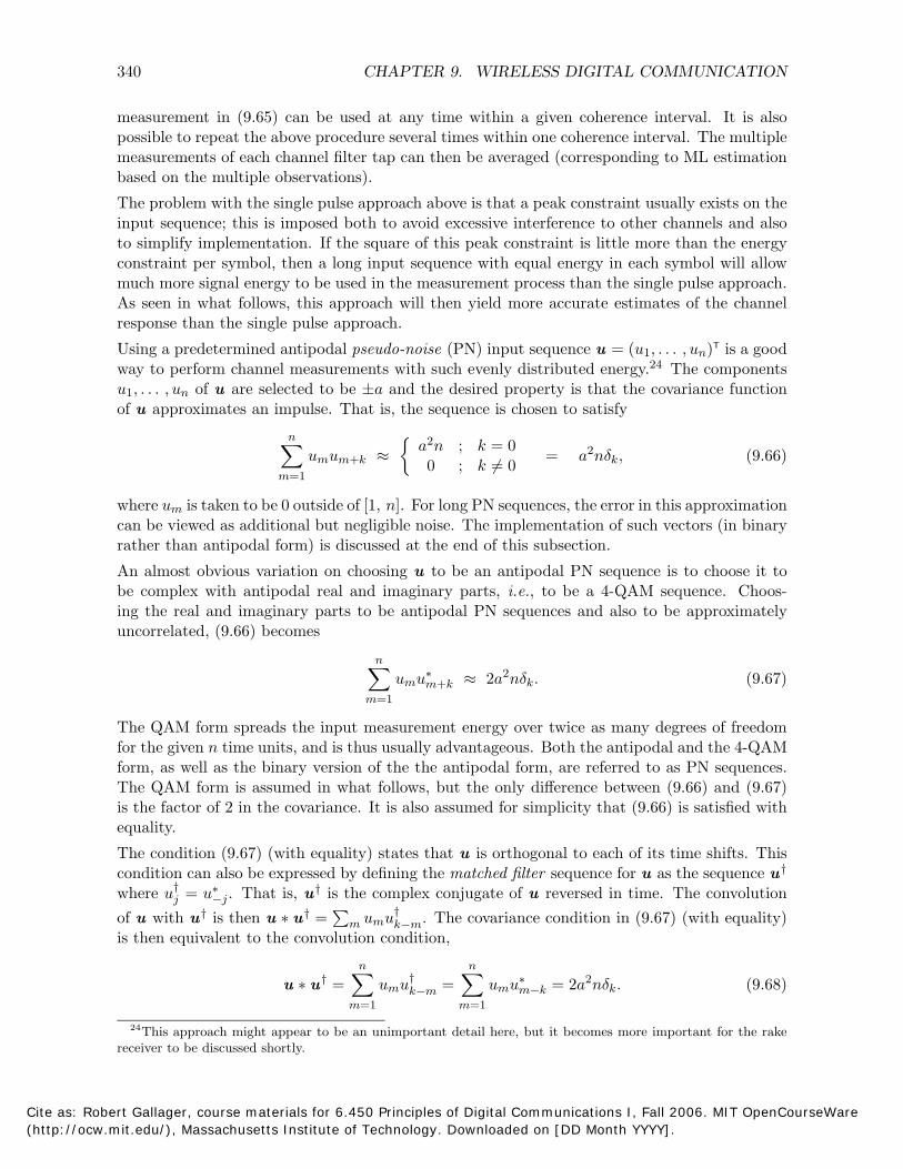
∑
∑ ∑ ∑
340 CHAPTER 9. WIRELESS DIGITAL COMMUNICATION
measurement in (9.65) can be used at any time within a given coherence interval. It is also possible to repeat the above procedure several times within one coherence interval. The multiple measurements of each channel filter tap can then be averaged (corresponding to ML estimation based on the multiple observations).
The problem with the single pulse approach above is that a peak constraint usually exists on the input sequence; this is imposed both to avoid excessive interference to other channels and also to simplify implementation. If the square of this peak constraint is little more than the energy constraint per symbol, then a long input sequence with equal energy in each symbol will allow much more signal energy to be used in the measurement process than the single pulse approach. As seen in what follows, this approach will then yield more accurate estimates of the channel response than the single pulse approach.
Using a predetermined antipodal pseudo-noise (PN) input sequence u = (u1, . . . , un)T is a good way to perform channel measurements with such evenly distributed energy.24 The components u1, . . . , un of u are selected to be ±a and the desired property is that the covariance function of u approximates an impulse. That is, the sequence is chosen to satisfy
n {∑ 2
umum+k a n ; k = 0
= a 2nδk, (9.66)≈ 0 ; k = 0
m=1 �
where um is taken to be 0 outside of [1, n]. For long PN sequences, the error in this approximation can be viewed as additional but negligible noise. The implementation of such vectors (in binary rather than antipodal form) is discussed at the end of this subsection.
An almost obvious variation on choosing u to be an antipodal PN sequence is to choose it to be complex with antipodal real and imaginary parts, i.e., to be a 4-QAM sequence. Choosing the real and imaginary parts to be antipodal PN sequences and also to be approximately uncorrelated, (9.66) becomes
n
umu∗ ≈ 2a 2nδk. (9.67)m+k m=1
The QAM form spreads the input measurement energy over twice as many degrees of freedom for the given n time units, and is thus usually advantageous. Both the antipodal and the 4-QAM form, as well as the binary version of the the antipodal form, are referred to as PN sequences. The QAM form is assumed in what follows, but the only difference between (9.66) and (9.67) is the factor of 2 in the covariance. It is also assumed for simplicity that (9.66) is satisfied with equality.
The condition (9.67) (with equality) states that u is orthogonal to each of its time shifts. This condition can also be expressed by defining the matched filter sequence for u as the sequence u†
where u† = u∗ That is, u† is the complex conjugate of u reversed in time. The convolution j −j .
of u with u† is then u ∗ u† = m umu†k−m. The covariance condition in (9.67) (with equality)
is then equivalent to the convolution condition,
n n
u ∗ u† = umu† = umu∗ = 2a 2nδk. (9.68)k−m m−k m=1 m=1
24This approach might appear to be an unimportant detail here, but it becomes more important for the rake receiver to be discussed shortly.
Cite as: Robert Gallager, course materials for 6.450 Principles of Digital Communications I, Fall 2006. MIT OpenCourseWare (http://ocw.mit.edu/), Massachusetts Institute of Technology. Downloaded on [DD Month YYYY].

∑
∑ ∑ ∑ ∑
9.7. CHANNEL MEASUREMENT 341
Let the complex-valued rv Gk,m be the value of the kth channel tap at time m. The channel output at time m for the input sequence u (before adding noise) is the convolution
n−1
Vm′ = Gk,mum−k. (9.69)
k=0
Since u is zero outside of the interval [1, n], the noise-free output sequence V ′ is zero outside of [1, n+k0−1]. Assuming that the channel is random but unchanging during this interval, the kth tap can be expressed as the complex rv Gk. Correlating the channel output with u∗
1, , u∗n· · ·
results in the covariance at each epoch j given by
−j+n −j+n n−1
Cj′ = Vm
′ u∗ = Gkum−ku∗ (9.70)m+j m+j
m=−j+1 m=−j+1 k=0
n−1
= Gk(2a 2 n)δj+k = 2a 2nG−j . (9.71) k=0
Thus the result of correlation, in the absence of noise, is the set of channel filter taps, scaled and reversed in time.
It is easier to understand this by looking at the convolution of V ′ with u†. That is,
V ′ ∗ u† = (u ∗G) ∗ u† = (u ∗ u†) ∗G = 2a 2 nG.
This uses the fact that convolution of sequences (just like convolution of functions) is both associative and commutative. Note that the result of convolution with the matched filter is the time reversal of the result of correlation, and is thus simply a scaled replica of the channel taps. Finally note that the matched filter u† is zero outside of the interval [−n,−1]. Thus if we visualize implementing the measurement of the channel using such a discrete filter, we are assuming (conceptually) that the receiver time reference lags the transmitter time reference by at least n epochs.
With the addition of noise, the overall output is V = V ′ + Z , i.e., the output at epoch m is Vm = Vm
′ +Zm. Thus the convolution of the noisy channel output with the matched filter u† is given by
V ∗ u† = V ′ ∗ u† + Z ∗ u† = 2a 2 nG + Z ∗ u†. (9.72)
After dividing by 2a2n, the kth component of this vector equation is
1 ∑ Vmu† = Gk + Ψk, (9.73)
2a2n k−m m
where Ψk is defined as the complex random variable
1 ∑ Ψk = Zmu† . (9.74)
2a2n k−m m
This estimation procedure is illustrated in Figure 9.9.
Cite as: Robert Gallager, course materials for 6.450 Principles of Digital Communications I, Fall 2006. MIT OpenCourseWare (http://ocw.mit.edu/), Massachusetts Institute of Technology. Downloaded on [DD Month YYYY].
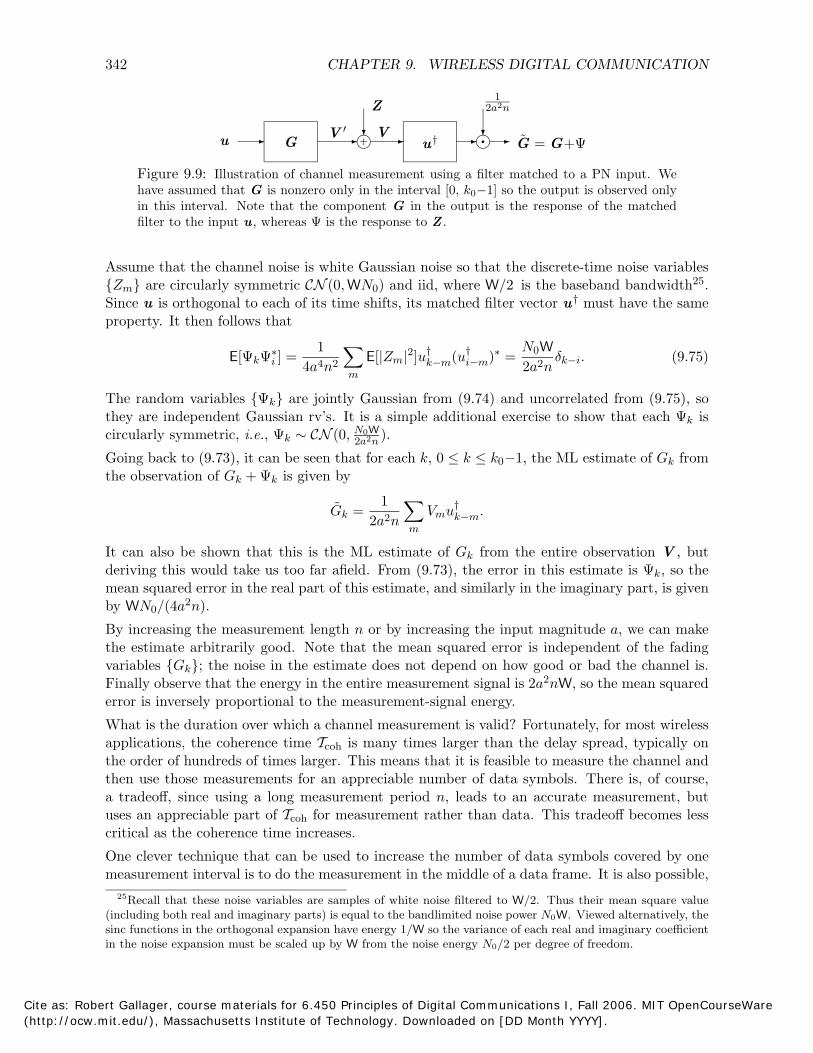
342 CHAPTER 9. WIRELESS DIGITAL COMMUNICATION
1 Z 2a2n
V� G V ′� �� � u†u � ��� � G = G+Ψ
Figure 9.9: Illustration of channel measurement using a filter matched to a PN input. We have assumed that G is nonzero only in the interval [0, k0−1] so the output is observed only in this interval. Note that the component G in the output is the response of the matched filter to the input u , whereas Ψ is the response to Z .
Assume that the channel noise is white Gaussian noise so that the discrete-time noise variables {Zm} are circularly symmetric CN (0,WN0) and iid, where W/2 is the baseband bandwidth25 . Since u is orthogonal to each of its time shifts, its matched filter vector u† must have the same property. It then follows that
1 ∑ 2]u
N0W E[ΨkΨi
∗] =4a4n2
E[|Zm| †k−m(u†
i−m)∗ =2a2n
δk−i. (9.75) m
The random variables {Ψk} are jointly Gaussian from (9.74) and uncorrelated from (9.75), so they are independent Gaussian rv’s. It is a simple additional exercise to show that each Ψk is circularly symmetric, i.e., Ψk ∼ CN (0, N0W).
2a2n
Going back to (9.73), it can be seen that for each k, 0 ≤ k ≤ k0−1, the ML estimate of Gk from the observation of Gk + Ψk is given by
Gk = 2a
1 2n
∑ Vmu†
k−m . m
It can also be shown that this is the ML estimate of Gk from the entire observation V , but deriving this would take us too far afield. From (9.73), the error in this estimate is Ψk, so the mean squared error in the real part of this estimate, and similarly in the imaginary part, is given by WN0/(4a2n).
By increasing the measurement length n or by increasing the input magnitude a, we can make the estimate arbitrarily good. Note that the mean squared error is independent of the fading variables {Gk}; the noise in the estimate does not depend on how good or bad the channel is. Finally observe that the energy in the entire measurement signal is 2a2nW, so the mean squared error is inversely proportional to the measurement-signal energy.
What is the duration over which a channel measurement is valid? Fortunately, for most wireless applications, the coherence time Tcoh is many times larger than the delay spread, typically on the order of hundreds of times larger. This means that it is feasible to measure the channel and then use those measurements for an appreciable number of data symbols. There is, of course, a tradeoff, since using a long measurement period n, leads to an accurate measurement, but uses an appreciable part of Tcoh for measurement rather than data. This tradeoff becomes less critical as the coherence time increases.
One clever technique that can be used to increase the number of data symbols covered by one measurement interval is to do the measurement in the middle of a data frame. It is also possible,
25Recall that these noise variables are samples of white noise filtered to W/2. Thus their mean square value (including both real and imaginary parts) is equal to the bandlimited noise power N0W. Viewed alternatively, the sinc functions in the orthogonal expansion have energy 1/W so the variance of each real and imaginary coefficient in the noise expansion must be scaled up by W from the noise energy N0/2 per degree of freedom.
Cite as: Robert Gallager, course materials for 6.450 Principles of Digital Communications I, Fall 2006. MIT OpenCourseWare (http://ocw.mit.edu/), Massachusetts Institute of Technology. Downloaded on [DD Month YYYY].
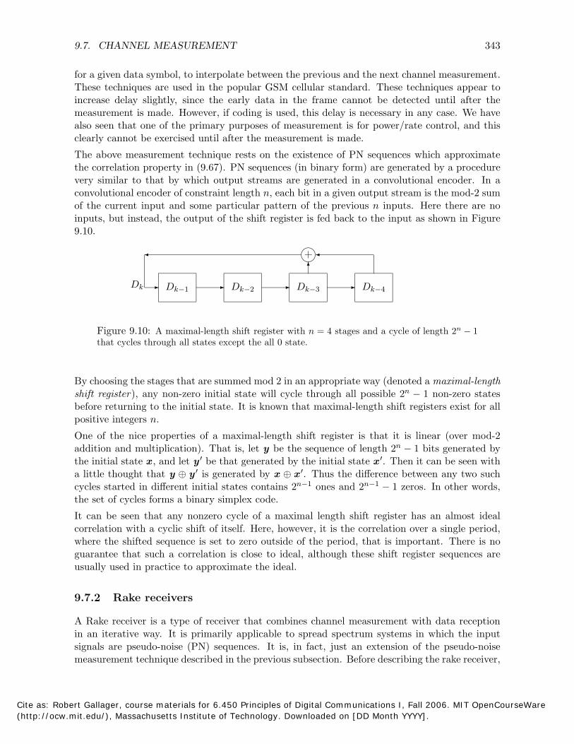
9.7. CHANNEL MEASUREMENT 343
for a given data symbol, to interpolate between the previous and the next channel measurement. These techniques are used in the popular GSM cellular standard. These techniques appear to increase delay slightly, since the early data in the frame cannot be detected until after the measurement is made. However, if coding is used, this delay is necessary in any case. We have also seen that one of the primary purposes of measurement is for power/rate control, and this clearly cannot be exercised until after the measurement is made.
The above measurement technique rests on the existence of PN sequences which approximate the correlation property in (9.67). PN sequences (in binary form) are generated by a procedure very similar to that by which output streams are generated in a convolutional encoder. In a convolutional encoder of constraint length n, each bit in a given output stream is the mod-2 sum of the current input and some particular pattern of the previous n inputs. Here there are no inputs, but instead, the output of the shift register is fed back to the input as shown in Figure 9.10.
Dk � Dk−3
�
�
Dk−4�Dk−2
�Dk−1�
� �
Figure 9.10: A maximal-length shift register with n = 4 stages and a cycle of length 2n − 1 that cycles through all states except the all 0 state.
By choosing the stages that are summed mod 2 in an appropriate way (denoted a maximal-length shift register), any non-zero initial state will cycle through all possible 2n − 1 non-zero states before returning to the initial state. It is known that maximal-length shift registers exist for all positive integers n.
One of the nice properties of a maximal-length shift register is that it is linear (over mod-2 addition and multiplication). That is, let y be the sequence of length 2n − 1 bits generated by the initial state x , and let y ′ be that generated by the initial state x ′. Then it can be seen with a little thought that y ⊕ y ′ is generated by x ⊕ x ′. Thus the difference between any two such cycles started in different initial states contains 2n−1 ones and 2n−1 − 1 zeros. In other words, the set of cycles forms a binary simplex code.
It can be seen that any nonzero cycle of a maximal length shift register has an almost ideal correlation with a cyclic shift of itself. Here, however, it is the correlation over a single period, where the shifted sequence is set to zero outside of the period, that is important. There is no guarantee that such a correlation is close to ideal, although these shift register sequences are usually used in practice to approximate the ideal.
9.7.2 Rake receivers
A Rake receiver is a type of receiver that combines channel measurement with data reception in an iterative way. It is primarily applicable to spread spectrum systems in which the input signals are pseudo-noise (PN) sequences. It is, in fact, just an extension of the pseudo-noise measurement technique described in the previous subsection. Before describing the rake receiver,
Cite as: Robert Gallager, course materials for 6.450 Principles of Digital Communications I, Fall 2006. MIT OpenCourseWare (http://ocw.mit.edu/), Massachusetts Institute of Technology. Downloaded on [DD Month YYYY].
�� �
�� � �� ��
���
���� �
��� �
344 CHAPTER 9. WIRELESS DIGITAL COMMUNICATION
it will be helpful to review binary detection, assuming that the channel is perfectly known and unchanging over the duration of the signal.
Let the input U be one of the two signals u0 = (u10 , , un
0 )T and u1 = (u11 , , un
1 )T. Denote· · · · · · the known channel taps as g = (g0, , gk0−1)T. Then the channel output, before the addition· · · of white noise, is either u0 ∗ g which we denote by b0, or u1 ∗ g , which we denote by b1. These convolutions are contained within the interval [1, n+k0−1]. After the addition of WGN, the output is either V = b0 + Z or V = b1 + Z . The detection problem is to decide, from observation of V , which of these two possibilities is more likely. The LLR for this detection problem is shown in Section 8.3.4 to be given by (8.26), repeated below,
LLR(v) = −‖v − b0‖2 + ‖v − b1‖2
N0
=2�(〈v , b0〉) − 2�(〈v , b1〉) − ‖b0‖2 + ‖b1‖2
(9.76)N0
It is shown in Exercise 9.17 that if u0 and u1 are ideal PN sequences, i.e., sequences that satisfy (9.68), then ‖b0‖2 = ‖b1‖2. The ML test then simplifies to
U=u0
0 1�(〈v ,u ∗ g〉) ≥ �(〈v ,u ∗ g〉). (9.77)<
U=u1
Finally, for i = 0, 1, the inner product 〈v ,u i ∗ g〉 is simply the output at epoch 0 when v is the input to a filter matched to u i ∗ g . The filter matched to u i ∗ g , however, is just the filter matched to u i convolved with the filter matched to g . The block diagram for this is shown in Figure 9.11.
Z u1 �
� �
(u1)† � g † �
b0 or b1 �v � b†� ��� 1g Decision
� �
(u0)† � g † 0 � ���u
b†0Figure 9.11: Detection for binary signals passed through a known filter g . The real parts of
the inputs entering the decision box at epoch 0 are compared. U=u0 if the real part of the lower input is larger, and U = u1 is chosen otherwise.
If the signals above are PN sequences, there is a great similarity between figures 9.9 and 9.11. In particular, if u0 is sent, then the output of the matched filter (u0)†, i.e., the first part of the lower matched filter, will be 2a2ng in the absence of noise. Note that g is a vector, meaning that the noise-free output at epoch k is 2a2ngk Similarly, if u1 is sent, then the noise-free output of the first part of the upper matched filter, at epoch k, will be a2ngk. The decision is made at receiver time 0 after the sequence 2a2ng , along with noise, passes through the unrealizable filter g †. These unrealizable filters are made realizable by the delay in receiver timing relative to transmitter timing.
Cite as: Robert Gallager, course materials for 6.450 Principles of Digital Communications I, Fall 2006. MIT OpenCourseWare (http://ocw.mit.edu/), Massachusetts Institute of Technology. Downloaded on [DD Month YYYY].
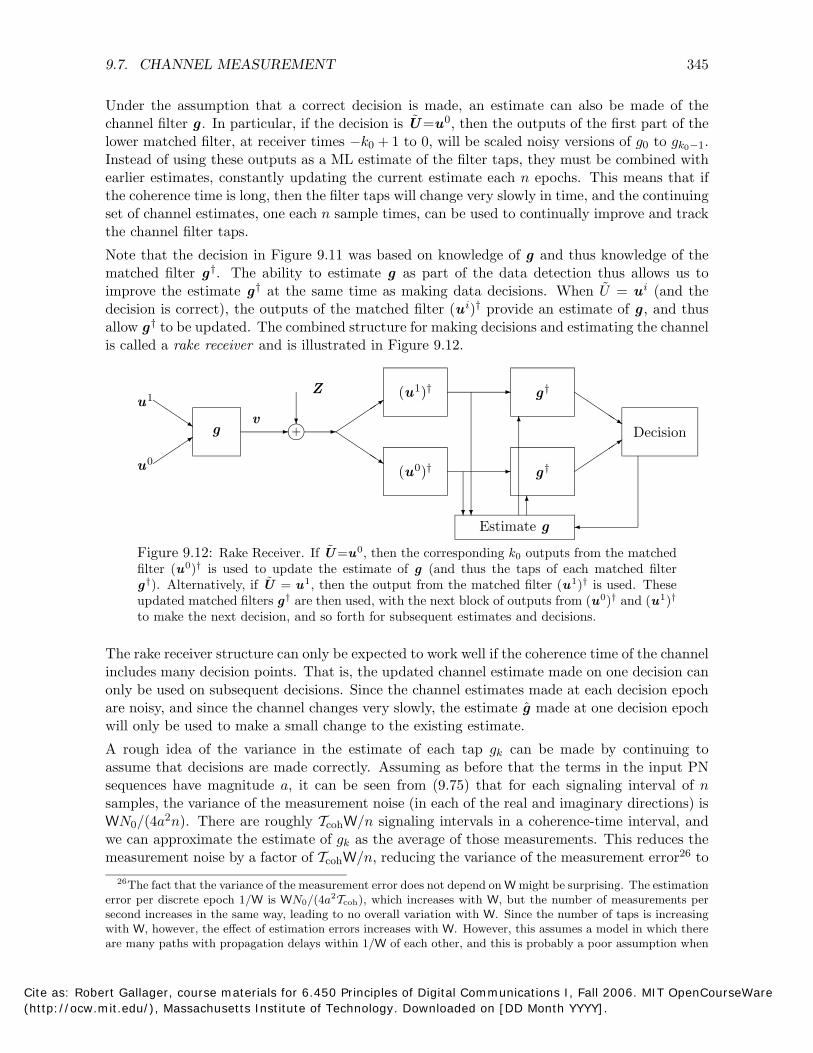
�� �
�� � � � ��
� ��� �
���� �
9.7. CHANNEL MEASUREMENT 345
Under the assumption that a correct decision is made, an estimate can also be made of the channel filter g . In particular, if the decision is U=u0, then the outputs of the first part of the lower matched filter, at receiver times −k0 + 1 to 0, will be scaled noisy versions of g0 to gk0−1. Instead of using these outputs as a ML estimate of the filter taps, they must be combined with earlier estimates, constantly updating the current estimate each n epochs. This means that if the coherence time is long, then the filter taps will change very slowly in time, and the continuing set of channel estimates, one each n sample times, can be used to continually improve and track the channel filter taps.
Note that the decision in Figure 9.11 was based on knowledge of g and thus knowledge of the matched filter g †. The ability to estimate g as part of the data detection thus allows us to
iimprove the estimate g † at the same time as making data decisions. When U = u (and the decision is correct), the outputs of the matched filter (u i)† provide an estimate of g , and thus allow g † to be updated. The combined structure for making decisions and estimating the channel is called a rake receiver and is illustrated in Figure 9.12.
u1�
0�u
v g
Z
(u0)† �
�
g † �����
(u1)† �
�
g † �����
Decision
�Estimate g
�
�
Figure 9.12: Rake Receiver. If U=u0, then the corresponding k0 outputs from the matched filter (u0)† is used to update the estimate of g (and thus the taps of each matched filter g†). Alternatively, if U = u1, then the output from the matched filter (u1)† is used. These updated matched filters g† are then used, with the next block of outputs from (u0)† and (u1)†
to make the next decision, and so forth for subsequent estimates and decisions.
The rake receiver structure can only be expected to work well if the coherence time of the channel includes many decision points. That is, the updated channel estimate made on one decision can only be used on subsequent decisions. Since the channel estimates made at each decision epoch are noisy, and since the channel changes very slowly, the estimate g made at one decision epoch will only be used to make a small change to the existing estimate.
A rough idea of the variance in the estimate of each tap gk can be made by continuing to assume that decisions are made correctly. Assuming as before that the terms in the input PN sequences have magnitude a, it can be seen from (9.75) that for each signaling interval of n samples, the variance of the measurement noise (in each of the real and imaginary directions) is WN0/(4a2n). There are roughly TcohW/n signaling intervals in a coherence-time interval, and we can approximate the estimate of gk as the average of those measurements. This reduces the measurement noise by a factor of TcohW/n, reducing the variance of the measurement error26 to
26The fact that the variance of the measurement error does not depend on W might be surprising. The estimation error per discrete epoch 1/W is WN0/(4a 2 Tcoh), which increases with W, but the number of measurements per second increases in the same way, leading to no overall variation with W. Since the number of taps is increasing with W, however, the effect of estimation errors increases with W. However, this assumes a model in which there are many paths with propagation delays within 1/W of each other, and this is probably a poor assumption when
Cite as: Robert Gallager, course materials for 6.450 Principles of Digital Communications I, Fall 2006. MIT OpenCourseWare (http://ocw.mit.edu/), Massachusetts Institute of Technology. Downloaded on [DD Month YYYY].
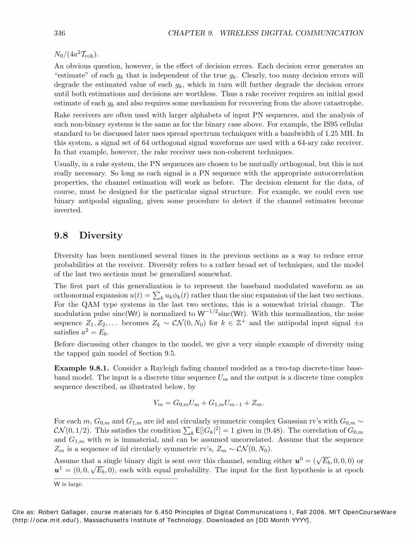
∑
∑
346 CHAPTER 9. WIRELESS DIGITAL COMMUNICATION
N0/(4a2coh).T
An obvious question, however, is the effect of decision errors. Each decision error generates an “estimate” of each gk that is independent of the true gk. Clearly, too many decision errors will degrade the estimated value of each gk, which in turn will further degrade the decision errors until both estimations and decisions are worthless. Thus a rake receiver requires an initial good estimate of each gk and also requires some mechanism for recovering from the above catastrophe.
Rake receivers are often used with larger alphabets of input PN sequences, and the analysis of such non-binary systems is the same as for the binary case above. For example, the IS95 cellular standard to be discussed later uses spread spectrum techniques with a bandwidth of 1.25 MH. In this system, a signal set of 64 orthogonal signal waveforms are used with a 64-ary rake receiver. In that example, however, the rake receiver uses non-coherent techniques.
Usually, in a rake system, the PN sequences are chosen to be mutually orthogonal, but this is not really necessary. So long as each signal is a PN sequence with the appropriate autocorrelation properties, the channel estimation will work as before. The decision element for the data, of course, must be designed for the particular signal structure. For example, we could even use binary antipodal signaling, given some procedure to detect if the channel estimates become inverted.
9.8 Diversity
Diversity has been mentioned several times in the previous sections as a way to reduce error probabilities at the receiver. Diversity refers to a rather broad set of techniques, and the model of the last two sections must be generalized somewhat.
The first part of this generalization is to represent the baseband modulated waveform as an orthonormal expansion u(t) = k ukφk(t) rather than the sinc expansion of the last two sections. For the QAM type systems in the last two sections, this is a somewhat trivial change. The modulation pulse sinc(Wt) is normalized to W−1/2sinc(Wt). With this normalization, the noise sequence Z1, Z2, . . . becomes Zk ∼ CN (0, N0) for k ∈ Z+ and the antipodal input signal ±a satisfies a2 = Eb.
Before discussing other changes in the model, we give a very simple example of diversity using the tapped gain model of Section 9.5.
Example 9.8.1. Consider a Rayleigh fading channel modeled as a two-tap discrete-time baseband model. The input is a discrete time sequence Um and the output is a discrete time complex sequence described, as illustrated below, by
Vm = G0,mUm + G1,mUm−1 + Zm.
For each m, G0,m and G1,m are iid and circularly symmetric complex Gaussian rv’s with G0,m ∼ CN (0, 1/2). This satisfies the condition k E[|Gk|2] = 1 given in (9.48). The correlation of G0,m
and G1,m with m is immaterial, and can be assumed uncorrelated. Assume that the sequence Zm is a sequence of iid circularly symmetric rv’s, Zm ∼ CN (0, N0).
Assume that a single binary digit is sent over this channel, sending either u0 = (√
Eb, 0, 0, 0) or u1 = (0, 0,
√Eb, 0), each with equal probability. The input for the first hypothesis is at epoch
W is large.
Cite as: Robert Gallager, course materials for 6.450 Principles of Digital Communications I, Fall 2006. MIT OpenCourseWare (http://ocw.mit.edu/), Massachusetts Institute of Technology. Downloaded on [DD Month YYYY].
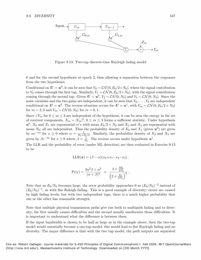
∑ �
9.8. DIVERSITY 347
Input Um Um−1
���� �� �� �� G1,mG0,m
� � �
Zm � � +� � Vm
Figure 9.13: Two-tap discrete-time Rayleigh fading model
0 and for the second hypothesis at epoch 2, thus allowing a separation between the responses from the two hypotheses.
Conditional on U = u0, it can be seen that V0 ∼ CN (0, Eb/2+N0), where the signal contribution to V0 comes through the first tap. Similarly, V1 ∼ CN (0, Eb/2+N0), with the signal contribution coming through the second tap. Given U = u0 , V2 ∼ CN (0, N0) and V3 ∼ CN (0, N0). Since the noise variables and the two gains are independent, it can be seen that V0, . . . , V3 are independent conditional on U = u0. The reverse situation occurs for U = u1, with Vm ∼ CN (0, Eb/2 + N0) for m = 2, 3 and Vm ∼ CN (0, N0) for m = 0, 1.
Since ∠Vm for 0 ≤ m ≤ 3 are independent of the hypothesis, it can be seen the energy in the set of received components, Xm = Vm
2 , 0 ≤ m ≤ 3 forms a sufficient statistic. Under hypothesis 0
| |u , X0 and X1 are exponential rv’s with mean Eb/2 + N0 and X2 and X3 are exponential with mean N0; all are independent. Thus the probability density of X0 and X1 (given u0) are given by αe−αx for x ≥ 0 where α = 1 . Similarly, the probability density of X2 and X3 areN0+Eb/2
given by βe−βx for x ≥ 0 where β = 1 . The reverse occurs under hypothesis u1 .N0
The LLR and the probability of error (under ML detection) are then evaluated in Exercise 9.13 to be
LLR(x ) = (β − α)(x0+x1−x2−x3) .
4 + 3Eb
Pr(e) = (α + β)3
= ( Eb
)3 . 2 +
3α2β + α32N0
2N0
Note that as Eb/N0 becomes large, the error probability approaches 0 as (Eb/N0)−2 instead of (Eb/N0)−1, as with flat Raleigh fading. This is a good example of diversity; errors are caused by high fading levels, but with two independent taps, there is a much higher probability that one or the other has reasonable strength.
Note that multiple physical transmission paths give rise both to multipath fading and to diversity; the first usually causes difficulties and the second usually ameliorates those difficulties. It is important to understand what the difference is between them.
If the input bandwidth is chosen to be half as large as in the example above, then the two-tap model would essentially become a one-tap model; this would lead to flat Rayleigh fading and no diversity. The major difference is that with the two tap model, the path outputs are separated
Cite as: Robert Gallager, course materials for 6.450 Principles of Digital Communications I, Fall 2006. MIT OpenCourseWare (http://ocw.mit.edu/), Massachusetts Institute of Technology. Downloaded on [DD Month YYYY].
348 CHAPTER 9. WIRELESS DIGITAL COMMUNICATION
into two groups and the effect of each can be observed separately. With the one tap model, the paths are all combined, since there are no longer independently observable sets of paths.
It is also interesting to compare the diversity receiver above with a receiver that could make use of channel measurements. If the tap values were known, then an ML detector would involve a matched filter on the channel taps, as in Figure 9.12. In terms of the particular input in the above exercise, this would weight the outputs from the two channel taps according to the magnitude of the tap, whereas the diversity receiver above weights them equally. In other words, the diversity detector above doesn’t do quite the right thing given known tap values, but it certainly is a large improvement over narrow band transmission.
The type of diversity used above is called time diversity since it makes use of the delay between different sets of paths. The analysis above hides a major part of the benefit to be gained by time diversity. For example, in the familiar reflecting wall example, there are only two paths. If the signal bandwidth is large enough that the response comes on different taps (or if the receiver measures the time delay on each path), then the fading will be eliminated.
It appears that many wireless situations, particularly those in cellular and local area networks, contain a relatively small number of significant coherent paths, and if the bandwidth is large enough to resolve these paths, then the gain is far greater than that indicated in the example above.
The diversity receiver above can be generalized to other discrete models for wireless channels. For example, the frequency band could be separated into segments separated by the coherence frequency, thus getting roughly independent fading in each and the ability to separate the outputs in each of those bands. Diversity in frequency is somewhat different than diversity in time, since it doesn’t allow the resolution of paths of different delays.
Another way to achieve diversity is through multiple antennas at the transmitter and receiver. Note that multiple antennas at the receiver allow the full received power available at one antenna to be received at each antenna, rather than splitting the power as occurs with time diversity or frequency diversity. For all of these more general ways to achieve diversity, the input and output should obviously be represented by the appropriate orthonormal expansions to bring out the diversity terms.
The two-tap example above can be easily extended to an arbitrary number of taps. Assume the model of Figure 9.13 modified to have L taps, G0,m, . . . , GL−1,m satisfying Gk,m ∼
0CN (0, 1/L) for 0 ≤ k ≤ L − 1. The input is assumed to be either u = (√
Eb, 0, . . . , 0) or u1 = (0, . . . , 0,
√Eb, 0, . . . , 0), where each of these 2L-tuples has zeros in all but one position,
namely position 0 for u0 and position L for u1. The energy in the set of received components, Xm = Vm
2 , 0 ≤ m ≤ 2L − 1, forms a sufficient statistic for the same reason as in the dual di| |0versity case. Under hypothesis u , X0, . . . , XL−1 are exponential rv’s with density α exp(−αx)
where α = 1 . Similarly, XL, . . . , X2L−1 are exponential rv’s with density β exp(−βx).N0+Eb/L
All are conditionally independent given u0. The reverse is true given hypothesis u1 .
It can be seen that the ML detection rule is to choose u0 if ∑L−1 X
∑2L−1 X and to m=0 m ≥ m=L m
choose u1 otherwise. Exercise 9.14 then shows that the error probability is
Pr(e) = 2∑L−1 (2L − 1
) p (1 − p)2L−1− .
=L
Cite as: Robert Gallager, course materials for 6.450 Principles of Digital Communications I, Fall 2006. MIT OpenCourseWare (http://ocw.mit.edu/), Massachusetts Institute of Technology. Downloaded on [DD Month YYYY].
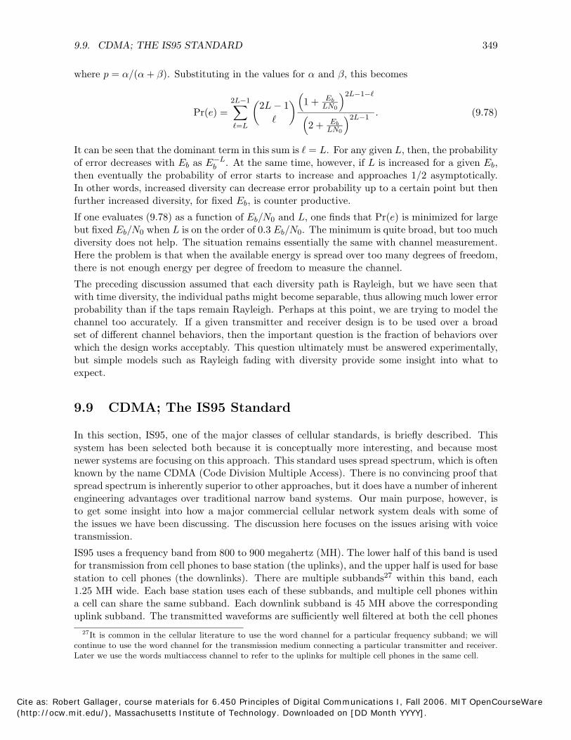
9.9. CDMA; THE IS95 STANDARD 349
where p = α/(α + β). Substituting in the values for α and β, this becomes
2∑L−1 ( )( 1 + Eb
)2L−1−
LN0Pr(e) = 2L − 1 ( )2L−1
. (9.78) =L
2 + Eb LN0
It can be seen that the dominant term in this sum is = L. For any given L, then, the probability of error decreases with Eb as Eb
−L. At the same time, however, if L is increased for a given Eb, then eventually the probability of error starts to increase and approaches 1/2 asymptotically. In other words, increased diversity can decrease error probability up to a certain point but then further increased diversity, for fixed Eb, is counter productive.
If one evaluates (9.78) as a function of Eb/N0 and L, one finds that Pr(e) is minimized for large but fixed Eb/N0 when L is on the order of 0.3 Eb/N0. The minimum is quite broad, but too much diversity does not help. The situation remains essentially the same with channel measurement. Here the problem is that when the available energy is spread over too many degrees of freedom, there is not enough energy per degree of freedom to measure the channel.
The preceding discussion assumed that each diversity path is Rayleigh, but we have seen that with time diversity, the individual paths might become separable, thus allowing much lower error probability than if the taps remain Rayleigh. Perhaps at this point, we are trying to model the channel too accurately. If a given transmitter and receiver design is to be used over a broad set of different channel behaviors, then the important question is the fraction of behaviors over which the design works acceptably. This question ultimately must be answered experimentally, but simple models such as Rayleigh fading with diversity provide some insight into what to expect.
9.9 CDMA; The IS95 Standard
In this section, IS95, one of the major classes of cellular standards, is briefly described. This system has been selected both because it is conceptually more interesting, and because most newer systems are focusing on this approach. This standard uses spread spectrum, which is often known by the name CDMA (Code Division Multiple Access). There is no convincing proof that spread spectrum is inherently superior to other approaches, but it does have a number of inherent engineering advantages over traditional narrow band systems. Our main purpose, however, is to get some insight into how a major commercial cellular network system deals with some of the issues we have been discussing. The discussion here focuses on the issues arising with voice transmission.
IS95 uses a frequency band from 800 to 900 megahertz (MH). The lower half of this band is used for transmission from cell phones to base station (the uplinks), and the upper half is used for base station to cell phones (the downlinks). There are multiple subbands27 within this band, each 1.25 MH wide. Each base station uses each of these subbands, and multiple cell phones within a cell can share the same subband. Each downlink subband is 45 MH above the corresponding uplink subband. The transmitted waveforms are sufficiently well filtered at both the cell phones
27It is common in the cellular literature to use the word channel for a particular frequency subband; we will continue to use the word channel for the transmission medium connecting a particular transmitter and receiver. Later we use the words multiaccess channel to refer to the uplinks for multiple cell phones in the same cell.
Cite as: Robert Gallager, course materials for 6.450 Principles of Digital Communications I, Fall 2006. MIT OpenCourseWare (http://ocw.mit.edu/), Massachusetts Institute of Technology. Downloaded on [DD Month YYYY].
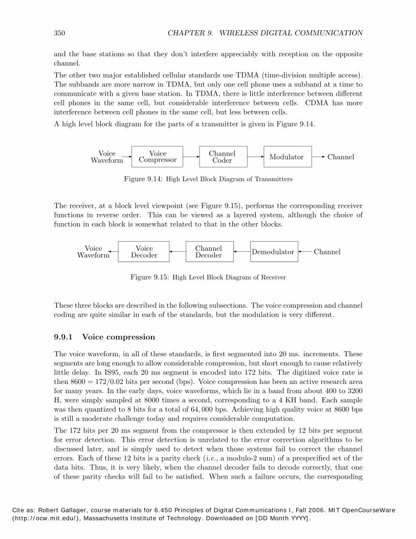
350 CHAPTER 9. WIRELESS DIGITAL COMMUNICATION
and the base stations so that they don’t interfere appreciably with reception on the opposite channel.
The other two major established cellular standards use TDMA (time-division multiple access).The subbands are more narrow in TDMA, but only one cell phone uses a subband at a time tocommunicate with a given base station. In TDMA, there is little interference between differentcell phones in the same cell, but considerable interference between cells. CDMA has moreinterference between cell phones in the same cell, but less between cells.
A high level block diagram for the parts of a transmitter is given in Figure 9.14.
Voice Waveform
� Compressor
Voice � Coder
Channel � Modulator � Channel
Figure 9.14: High Level Block Diagram of Transmitters
The receiver, at a block level viewpoint (see Figure 9.15), performs the corresponding receiver functions in reverse order. This can be viewed as a layered system, although the choice of function in each block is somewhat related to that in the other blocks.
Voice Waveform
� Decoder Voice �
Decoder Channel � Demodulator � Channel
Figure 9.15: High Level Block Diagram of Receiver
These three blocks are described in the following subsections. The voice compression and channel coding are quite similar in each of the standards, but the modulation is very different.
9.9.1 Voice compression
The voice waveform, in all of these standards, is first segmented into 20 ms. increments. These segments are long enough to allow considerable compression, but short enough to cause relatively little delay. In IS95, each 20 ms segment is encoded into 172 bits. The digitized voice rate is then 8600 = 172/0.02 bits per second (bps). Voice compression has been an active research area for many years. In the early days, voice waveforms, which lie in a band from about 400 to 3200 H, were simply sampled at 8000 times a second, corresponding to a 4 KH band. Each sample was then quantized to 8 bits for a total of 64, 000 bps. Achieving high quality voice at 8600 bps is still a moderate challenge today and requires considerable computation.
The 172 bits per 20 ms segment from the compressor is then extended by 12 bits per segment for error detection. This error detection is unrelated to the error correction algorithms to be discussed later, and is simply used to detect when those systems fail to correct the channel errors. Each of these 12 bits is a parity check (i.e., a modulo-2 sum) of a prespecified set of the data bits. Thus, it is very likely, when the channel decoder fails to decode correctly, that one of these parity checks will fail to be satisfied. When such a failure occurs, the corresponding
Cite as: Robert Gallager, course materials for 6.450 Principles of Digital Communications I, Fall 2006. MIT OpenCourseWare (http://ocw.mit.edu/), Massachusetts Institute of Technology. Downloaded on [DD Month YYYY].
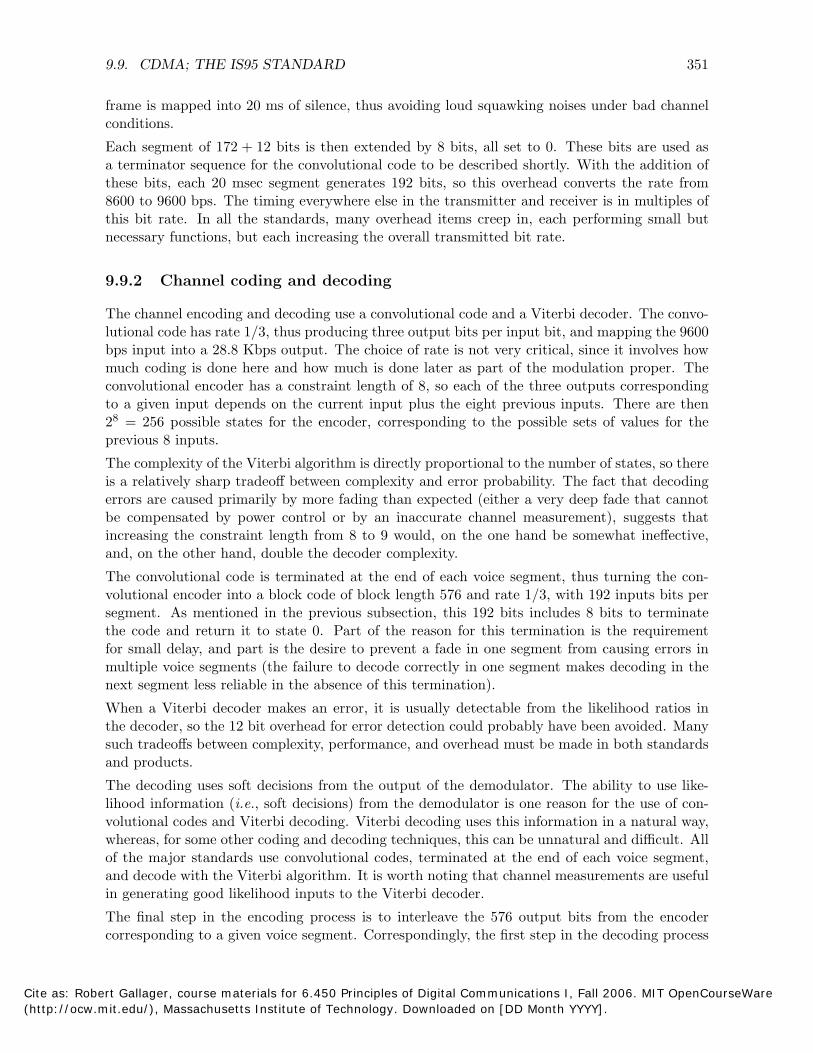
9.9. CDMA; THE IS95 STANDARD 351
frame is mapped into 20 ms of silence, thus avoiding loud squawking noises under bad channel conditions.
Each segment of 172 + 12 bits is then extended by 8 bits, all set to 0. These bits are used as a terminator sequence for the convolutional code to be described shortly. With the addition of these bits, each 20 msec segment generates 192 bits, so this overhead converts the rate from 8600 to 9600 bps. The timing everywhere else in the transmitter and receiver is in multiples of this bit rate. In all the standards, many overhead items creep in, each performing small but necessary functions, but each increasing the overall transmitted bit rate.
9.9.2 Channel coding and decoding
The channel encoding and decoding use a convolutional code and a Viterbi decoder. The convolutional code has rate 1/3, thus producing three output bits per input bit, and mapping the 9600 bps input into a 28.8 Kbps output. The choice of rate is not very critical, since it involves how much coding is done here and how much is done later as part of the modulation proper. The convolutional encoder has a constraint length of 8, so each of the three outputs corresponding to a given input depends on the current input plus the eight previous inputs. There are then 28 = 256 possible states for the encoder, corresponding to the possible sets of values for the previous 8 inputs.
The complexity of the Viterbi algorithm is directly proportional to the number of states, so there is a relatively sharp tradeoff between complexity and error probability. The fact that decoding errors are caused primarily by more fading than expected (either a very deep fade that cannot be compensated by power control or by an inaccurate channel measurement), suggests that increasing the constraint length from 8 to 9 would, on the one hand be somewhat ineffective, and, on the other hand, double the decoder complexity.
The convolutional code is terminated at the end of each voice segment, thus turning the convolutional encoder into a block code of block length 576 and rate 1/3, with 192 inputs bits per segment. As mentioned in the previous subsection, this 192 bits includes 8 bits to terminate the code and return it to state 0. Part of the reason for this termination is the requirement for small delay, and part is the desire to prevent a fade in one segment from causing errors in multiple voice segments (the failure to decode correctly in one segment makes decoding in the next segment less reliable in the absence of this termination).
When a Viterbi decoder makes an error, it is usually detectable from the likelihood ratios in the decoder, so the 12 bit overhead for error detection could probably have been avoided. Many such tradeoffs between complexity, performance, and overhead must be made in both standards and products.
The decoding uses soft decisions from the output of the demodulator. The ability to use likelihood information (i.e., soft decisions) from the demodulator is one reason for the use of convolutional codes and Viterbi decoding. Viterbi decoding uses this information in a natural way, whereas, for some other coding and decoding techniques, this can be unnatural and difficult. All of the major standards use convolutional codes, terminated at the end of each voice segment, and decode with the Viterbi algorithm. It is worth noting that channel measurements are useful in generating good likelihood inputs to the Viterbi decoder.
The final step in the encoding process is to interleave the 576 output bits from the encoder corresponding to a given voice segment. Correspondingly, the first step in the decoding process
Cite as: Robert Gallager, course materials for 6.450 Principles of Digital Communications I, Fall 2006. MIT OpenCourseWare (http://ocw.mit.edu/), Massachusetts Institute of Technology. Downloaded on [DD Month YYYY].

352 CHAPTER 9. WIRELESS DIGITAL COMMUNICATION
is to de-interleave the bits (actually the soft decisions) coming out of the demodulator. It can be seen without analysis that if the noise coming into a Viterbi decoder is highly correlated, then the Viterbi decoder, with its short constraint length, is more likely to make a decoding error than if the noise is independent. The next subsection will show that the noise from the demodulator is in fact highly correlated, and thus the interleaving breaks up this correlation. Figure 9.16 summarizes this channel encoding process.
8.6 Kbps � 12 bit 9.6 Kbps� 8 bit Conv. terminatorError det. 172 b/seg. 192 b/seg.
� Convolutional 28.8 Kbps � Inter 28.8 Kbps� Encoder leave 576 b/seg. 576 b/seg.
Figure 9.16: Block diagram of Channel Encoding
9.9.3 Viterbi decoding for fading channels
In order to get some sense of why the above convolutional code with Viterbi decoding will not work very well if the coding is followed by straight-forward binary modulation, suppose the pulse position modulation of Subsection 9.6.1 is used and the channel is represented by a single tap with Rayleigh fading. The resulting bandwidth is well within typical values of Fcoh, so the single tap model is reasonable. The coherence time is typically at least a msec, but in the absence of moving vehicles, it could easily be more than 20 msec.
This means that an entire 20 msec. segment of voice could easily be transmitted during a deep fade, and the convolutional encoder, even with interleaving within that 20 msec. would not be able to decode successfully. If the fading is much faster, the Viterbi decoder, with likelihood information on the incoming bits, would probably work fairly successfully, but that is not something that can be relied upon.
There are only three remedies for this situation. One is to send more power when the channel is faded. As shown in Exercise 9.11, however, if the input power compensates completely for the fading (i.e., the input power at time m is 1/|gm|2), then the expected input power is infinite. This means that, with finite average power, deep fades for prolonged periods cause outages.
The second remedy is diversity, in which each codeword is spread over enough coherence bandwidths or coherence-time intervals to achieve averaging over the channel fades. Using diversity over several coherence-time intervals causes delays proportional to the coherence time, which is usually unacceptable for voice. Diversity can be employed by using a bandwidth larger than the coherence frequency (this can be done using multiple taps in the tapped delay line model or multiple frequency bands).
The third remedy is the use of variable rate transmission. This is not traditional for voice, since the voice encoding traditionally produces a constant rate stream of input bits into the channel, and the delay constraint is too stringent to queue this input and transmit it when the channel is good. It would be possible to violate the source/channel separation principle and have the source produce “important bits” at one rate and “unimportant bits” at another rate. Then
Cite as: Robert Gallager, course materials for 6.450 Principles of Digital Communications I, Fall 2006. MIT OpenCourseWare (http://ocw.mit.edu/), Massachusetts Institute of Technology. Downloaded on [DD Month YYYY].
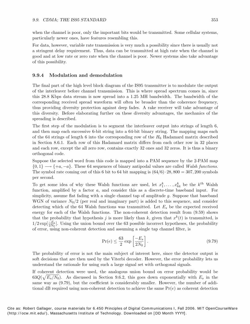
[ ]
√
9.9. CDMA; THE IS95 STANDARD 353
when the channel is poor, only the important bits would be transmitted. Some cellular systems, particularly newer ones, have features resembling this.
For data, however, variable rate transmission is very much a possibility since there is usually not a stringent delay requirement. Thus, data can be transmitted at high rate when the channel is good and at low rate or zero rate when the channel is poor. Newer systems also take advantage of this possibility.
9.9.4 Modulation and demodulation
The final part of the high level block diagram of the IS95 transmitter is to modulate the output of the interleaver before channel transmission. This is where spread spectrum comes in, since this 28.8 Kbps data stream is now spread into a 1.25 MH bandwidth. The bandwidth of the corresponding received spread waveform will often be broader than the coherence frequency, thus providing diversity protection against deep fades. A rake receiver will take advantage of this diversity. Before elaborating further on these diversity advantages, the mechanics of the spreading is described.
The first step of the modulation is to segment the interleaver output into strings of length 6, and then map each successive 6-bit string into a 64-bit binary string. The mapping maps each of the 64 strings of length 6 into the corresponding row of the H6 Hadamard matrix described in Section 8.6.1. Each row of this Hadamard matrix differs from each other row in 32 places and each row, except the all zero row, contains exactly 32 ones and 32 zeros. It is thus a binary orthogonal code.
Suppose the selected word from this code is mapped into a PAM sequence by the 2-PAM map {0, 1} −→ {+a,−a}. These 64 sequences of binary antipodal values are called Walsh functions. The symbol rate coming out of this 6 bit to 64 bit mapping is (64/6) 28, 800 = 307, 200 symbols ·per second.
To get some idea of why these Walsh functions are used, let x1k, . . . , xk be the kth Walsh 64
function, amplified by a factor a, and consider this as a discrete-time baseband input. For simplicity, assume flat fading with a single channel tap of amplitude g. Suppose that baseband WGN of variance N0/2 (per real and imaginary part) is added to this sequence, and consider detecting which of the 64 Walsh functions was transmitted. Let Es be the expected received energy for each of the Walsh functions. The non-coherent detection result from (9.59) shows that the probability that hypothesis j is more likely than k, given that xk(t) is transmitted, is 1/2 exp[−2N
E0
s ]. Using the union bound over the 63 possible incorrect hypotheses, the probability of error, using non-coherent detection and assuming a single tap channel filter, is
sPr(e) ≤ 63
exp −E
. (9.79)2 2N0
The probability of error is not the main subject of interest here, since the detector output is soft decisions that are then used by the Viterbi decoder. However, the error probability lets us understand the rationale for using such a large signal set with orthogonal signals.
If coherent detection were used, the analogous union bound on error probability would be 63Q( Es/N0). As discussed in Section 9.6.2, this goes down exponentially with Es in the same way as (9.79), but the coefficient is considerably smaller. However, the number of additional dB required using non-coherent detection to achieve the same Pr(e) as coherent detection
Cite as: Robert Gallager, course materials for 6.450 Principles of Digital Communications I, Fall 2006. MIT OpenCourseWare (http://ocw.mit.edu/), Massachusetts Institute of Technology. Downloaded on [DD Month YYYY].
354 CHAPTER 9. WIRELESS DIGITAL COMMUNICATION
decreases almost inversely with the exponent in (9.79). This means that by using a large number of orthogonal functions (64 in this case), we make the exponent in (9.79) large in magnitude, and thus approach (in dB terms) what could be achieved by coherent detection.
The argument above is incomplete, because Es is the transmitted energy per Walsh function. However, 6 binary digits are used to select each transmitted Walsh function. Thus, Eb in this case is Es/6 and (9.79) becomes
Pr(e) ≤ 63 exp(−3Eb/N0). (9.80)
This large signal set also avoids the 3 dB penalty for orthogonal signaling rather than antipodal signaling that we have seen for binary signal sets. Here the cost of orthogonality essentially lies in using an orthogonal code rather than the corresponding biorthogonal code with 7 bits of input and 128 codewords28 , i.e., a factor of 6/7 in rate.
A questionable issue here is that two codes (the convolutional code as an outer code, followed by the Walsh function code as an inner code) are used in place of a single code. There seems to be no clean analytical way of showing that this choice makes good sense over all choices of single or combined codes. On the other hand, each code is performing a rather different function. The Viterbi decoder is eliminating the errors caused by occasional fades or anomalies, and the Walsh functions allow non-coherent detection and also enable a considerable reduction in error probability because of the large orthogonal signal sets rather than binary transmission.
The modulation scheme in IS95 next spreads the above Walsh functions into an even wider bandwidth transmitted signal. The stream of binary digits out of the Hadamard encoder29 is combined with a pseudo-noise (PN) sequence at a rate of 1228.8 kbps, i.e., four PN bits for each signal bit. In essence, each bit of the 307.2 kbps stream out of the Walsh encoder is repeated four times (to achieve the 1228.8 kbps rate) and is then added mod-2 to the PN sequence. This further spreading provides diversity over the available 1.25 MH bandwidth.
The constraint length here is n = 42 binary digits, so the period of the cycle is 242 − 1 (about 41 days). We can ignore the difference between simplex and orthogonal, and simply regard each cycle as orthogonal to each other cycle. Since the cycle is so long, however, it is better to simply approximate each cycle as a sequence of iid binary digits. There are several other PN sequences used in the IS-95 standard, and this one, because of its constraint length, is called the “long PN sequence.” PN sequences have many interesting properties, but for us it is enough to view them as iid but also known to the receiver.
The initial state of the long PN sequence is used to distinguish between different cell phones, and in fact this initial state is the only part of the transmitter system that is specific to a particular cell phone.
The resulting binary stream, after adding the long PN sequence, is at a rate of 1.2288 Mbps. This stream is duplicated into two streams prior to being quadrature modulated onto a cosine and sine carrier. The cosine stream is added mod-2 to another PN-sequence (called the in-phase or I-PN) sequence at rate 1.2288 Mbps, and the sine stream is added mod-2 to another PN sequence called the quadrature or Q-PN sequence. The I-PN and Q-PN sequences are the same for all cell phones and help in demodulation.
28This biorthogonal code is called a (64, 7, 32) Reed Muller code in the coding literature 29We visualized mapping the Hadamard binary sequences by a 2PAM map into Walsh functions for simplicity.
For implementation, it is more convenient to maintain binary (0,1) sequences until the final steps in the modulation process are completed.
Cite as: Robert Gallager, course materials for 6.450 Principles of Digital Communications I, Fall 2006. MIT OpenCourseWare (http://ocw.mit.edu/), Massachusetts Institute of Technology. Downloaded on [DD Month YYYY].
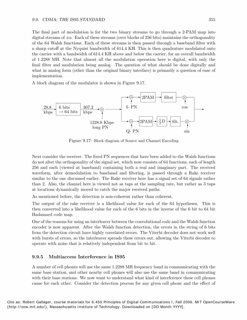
9.9. CDMA; THE IS95 STANDARD 355
The final part of modulation is for the two binary streams to go through a 2-PAM map into digital streams of ±a. Each of these streams (over blocks of 256 bits) maintains the orthogonality of the 64 Walsh functions. Each of these streams is then passed through a baseband filter with a sharp cutoff at the Nyquist bandwidth of 614.4 KH. This is then quadrature modulated onto the carrier with a bandwidth of 614.4 KH above and below the carrier, for an overall bandwidth of 1.2288 MH. Note that almost all the modulation operation here is digital, with only the final filter and modulation being analog. The question of what should be done digitally and what in analog form (other than the original binary interface) is primarily a question of ease of implementation.
A block diagram of the modulator is shown in Figure 9.17.
28.8 kbps
� 6 bits → 64 bits
307.2 kbps
�⊕�
1228.8 Kbps long PN
�
�⊕�
I- PN
� 2PAM � filter ⊗�
cos
�⊕�
� 2PAM� 1 2D � filt. ⊗
�
�
Q- PN sin
Figure 9.17: Block diagram of Source and Channel Encoding
Next consider the receiver. The fixed PN sequences that have been added to the Walsh functionsdo not alter the orthogonality of the signal set, which now consists of 64 functions, each of length256 and each (viewed at baseband) containing both a real and imaginary part. The receivedwaveform, after demodulation to baseband and filtering, is passed through a Rake receiversimilar to the one discussed earlier. The Rake receiver here has a signal set of 64 signals ratherthan 2. Also, the channel here is viewed not as taps at the sampling rate, but rather as 3 tapsat locations dynamically moved to catch the major received paths.
As mentioned before, the detection is non-coherent rather than coherent.
The output of the rake receiver is a likelihood value for each of the 64 hypotheses. This isthen converted into a likelihood value for each of the 6 bits in the inverse of the 6 bit to 64 bitHadamard code map.
One of the reasons for using an interleaver between the convolutional code and the Walsh functionencoder is now apparent. After the Walsh function detection, the errors in the string of 6 bitsfrom the detection circuit have highly correlated errors. The Viterbi decoder does not work wellwith bursts of errors, so the interleaver spreads these errors out, allowing the Viterbi decoder tooperate with noise that is relatively independent from bit to bit.
9.9.5 Multiaccess Interference in IS95
A number of cell phones will use the same 1.2288 MH frequency band in communicating with the same base station, and other nearby cell phones will also use the same band in communicating with their base stations. We now want to understand what kind of interference these cell phones cause for each other. Consider the detection process for any given cell phone and the effect of
Cite as: Robert Gallager, course materials for 6.450 Principles of Digital Communications I, Fall 2006. MIT OpenCourseWare (http://ocw.mit.edu/), Massachusetts Institute of Technology. Downloaded on [DD Month YYYY].
[ ]
356 CHAPTER 9. WIRELESS DIGITAL COMMUNICATION
the interference from the other cell phones.
Since each cell phone uses a different phase of the long PN sequence, the PN sequences from the interfering cell phones can be modeled as random iid binary streams. Since each of these streams is modeled as iid, the mod-2 addition of the PN stream and the data is still an iid stream of binary digits. If the filter used before transmission is very sharp (which it is, since the 1.2288 MH bands are quite close together), the Nyquist pulses can be approximated by sinc pulses. It also makes sense to model the sample clock of each interfering cell phone as being uniformly distributed. This means that the interfering cell phones can be modeled as being wide sense stationary with a flat spectrum over the 1.2288 MH band.
The more interfering cell phones there are in the same frequency band, the more interference there is, but also, since these interfering signals are independent of each other, we can invoke the central limit theorem to see that this aggregate interference will be approximately Gaussian.
To get some idea of the effect of the interference, assume that each interfering cell phone is received at the same baseband energy per information bit given by Eb. Since there are 9600 information bits per second entering the encoder, the power in the interfering waveform is then 9600Eb. This noise is evenly spread over 2,457,600 dimensions per second, so is (4800/2.4576 ×106)Eb = Eb/512 per dimension. Thus the noise per dimension is increased from N0/2 to (N0/2 + kEb/512) where k is the number of interferers. With this change, (9.80) becomes
63 −3EbPr(e) ≤ 2
exp N0 + kEb/256
. (9.81)
In reality, the interfering cell phones are received with different power levels, and because of this, the system uses a fairly elaborate system of power control to attempt to equalize the received powers of the cell phones being received at a given base station. Those cell phones being received at other base stations presumably have lower power at the given base station, and thus cause less interference. It can be seen that with a large set of interferers, the assumption that they form a Gaussian process is even better than with a single interferer.
The factor of 256 in (9.81) is due to the spreading of the waveforms (sending them in a bandwidth of 1.2288 MH rather than in a narrow band. This spreading, of course, is also the reason why appreciable numbers of other cell phones must use the same band. Since voice users are typically silent half the time while in a conversation, and the cell phone need send no energy during these silent periods, the number of tolerable interferers is doubled.
The other types of cellular systems (GSM and TDMA) attempt to keep the interfering cell phones in different frequency bands and time slots. If successful, this is, of course, preferable to CDMA, since there is then no interference rather than the limited interference in (9.81). The difficulty with these other schemes is that frequency slots and time slots must be reused by cell phones going to other cell stations (although preferably not by cell phones connected with neighboring cell stations). The need to avoid slot re-use between neighboring cells leads to very complex algorithms for allocating re-use patterns between cells, and these algorithms cannot make use of the factor of 2 due to users being quiet half the time.
Because these transmissions are narrow band, when interference occurs, it is not attenuated by a factor of 256 as in (9.81). Thus the question boils down to whether it is preferable to have a large number of small interferers or a small number of larger interferers. This, of course, is only one of the issues that differ between CDMA systems and narrow band systems. For example, narrow band systems cannot make use of rake receivers, although they can make use of many techniques developed over the years for narrow band transmission.
Cite as: Robert Gallager, course materials for 6.450 Principles of Digital Communications I, Fall 2006. MIT OpenCourseWare (http://ocw.mit.edu/), Massachusetts Institute of Technology. Downloaded on [DD Month YYYY].
∫
9.10. SUMMARY OF WIRELESS COMMUNICATION 357
9.10 Summary of Wireless Communication
Wireless communication differs from wired communication primarily in the time-varying nature of the channel and the interference from other wireless users. The time-varying nature of the channel is the more technologically challenging of the two, and has been the primary focus of this chapter.
Wireless channels frequently have multiple electromagnetic paths of different lengths from transmitter to receiver and thus the receiver gets multiple copies of the transmitted waveform at slightly different delays. If this were the only problem, then the channel could be represented as a linear time-invariant (LTI) filter with the addition of noise, and this could be treated as a relatively minor extension to the non-filtered channels with noise studied in earlier chapters.
The problem that makes wireless communication truly different is the fact that the different electromagnetic paths are also sometimes moving with respect to each other, thus giving rise to different Doppler shifts on different paths.
Section 9.3 showed that these multiple paths with varying Doppler shifts lead to an input/output model which, in the absence of noise, is modeled as a linear time-varying (LTV) filter h(τ, t), which is the response at time t to an impulse τ seconds earlier. This has a time varying system function h(f, t) which, for each fixed t, is the Fourier transform of h(τ, t). These LTV filters behave in a somewhat similar fashion to the familiar LTI filters. In particular, the channel input x(t) and noise-free output y(t) are related by the convolution equation, y(t) = h(τ, t)x(t−τ) dτ . Also, y(t), for each fixed t, is the inverse Fourier transform of x(f)h(f, t). The major difference is that y(f) is not equal to x(f)h(f, t) unless h(f, t) is non-varying in t.
The major parameters of a wireless channel (at a given carrier frequency fc) are the Doppler spread D and the time spread L. The Doppler spread is the difference between the largest and smallest significant Doppler shift on the channel (at fc). It was shown to be twice the bandwidth of |h(fc, t)| viewed as a function of t. Similarly, L is the time spread between the longest and shortest multipath delay (at a fixed output time t0). It was shown to be twice the ‘bandwidth’ of |h(f, t0)| viewed as a function of f .
1The coherence time Tcoh and coherence frequency Fcoh were defined as Tcoh = 2D and Fcoh = 1 . Qualitatively, these parameters represent the duration of multipath fades in time and the 2L
duration over frequency respectively. Fades, as their name suggests, occur gradually, both in time and frequency, so these parameters represent duration only in an order-of-magnitude sense.
As shown in Section 9.4, these bandpass models of wireless channels can be converted to baseband models and then converted to discrete time models. The relation between the bandpass and baseband model is quite similar to that for non-fading channels. The discrete time model relies on the sampling theorem, and, while mathematically correct, can somewhat distort the view of channels with a small number of paths, sometimes yielding only one tap, and sometimes yielding many more taps than paths. Nonetheless this model is so convenient for acquiring insight about wireless channels that it is widely used, particularly among those who dislike continuous-time models.
Section 9.5 then breaks the link with electromagnetic models and views the baseband tapped delay line model probabilistically. At the same time, WGN is added. A one-tap model corresponds to situations where the transmission bandwidth is narrow relative to the coherence frequency Fcoh and multitap models correspond to the opposite case. We generally model the individual taps as being Rayleigh faded, corresponding to a large number of small independent
Cite as: Robert Gallager, course materials for 6.450 Principles of Digital Communications I, Fall 2006. MIT OpenCourseWare (http://ocw.mit.edu/), Massachusetts Institute of Technology. Downloaded on [DD Month YYYY].
{ } { }
358 CHAPTER 9. WIRELESS DIGITAL COMMUNICATION
paths in the corresponding delay range. Several other models, including the Rician model and non-coherent deterministic model, were analyzed, but physical channels have such variety that these models only provide insight into the types of behavior to expect. The modeling issues are quite difficult here, and our point of view has been to analyze the consequences of a few very simple models.
Consistent with the above philosophy, Section 9.6 analyzes a single tap model with Rayleigh fading. The classical Rayleigh fading error probability, using binary orthogonal signals and no knowledge of the channel amplitude or phase, is calculated to be 1/[2 + Eb/N0]. The classical error probability for non-coherent detection, where the receiver knows the channel magnitude but not the phase, is also calculated and compared with the coherent result as derived for non-faded channels. For large Eb/N0, the results are very similar, saying that knowledge of the phase is not very important in that case. However, the non-coherent detector does not use the channel magnitude in detection, showing that detection in Rayleigh fading would not be improved by knowledge of the channel magnitude.
The conclusion from this study is that reasonably reliable communication for wireless channels needs diversity or coding or needs feedback with rate or power control. With Lth order diversity in Rayleigh fading, it was shown that error probability tends to 0 as (Eb/4N0)−L for large Eb/N0. If the magnitude of the various diversity paths are known, then the error probability can be made still smaller.
Knowledge of the channel as it varies can be helpful in two ways. One is to reduce the error probability when coding and/or diversity are used, and the other is to exercise rate control or power control at the transmitter. Section 9.7 analyzes various channel measurement techniques, including direct measurement by sending known probing sequences and measurement using rake receivers. These are both widely used and effective tools.
Finally, all of the above analysis and insight about wireless channels is brought to bear in Section 9.9, which describes the IS95 CDMA cellular system. In fact, this section illustrates most of the major topics throughout this text.
9A Appendix: Error probability for non-coherent detection
Under hypothesis U=(a, 0), is a Rician random variable R which has the density30|V0| { } ( ) r r2 + a2g2 rag
fR(r) = WN0/2
exp − WN0
I0 WN0/2
, r ≥ 0, (9.82)
where I0 is the modified Bessel function of zeroth order. Conditional on U=(0, a), |V1| has the same density, so the likelihood ratio is
f [(|v0|, |v1|) |U=(a, 0)] =
I0(2|v0|ag/WN0) . (9.83)
f [(|v0|, |v1|) |U=(0, a)] I0(2|v1|ag/WN0)
I0 is known to be monotonic increasing in its argument, which verifies that the maximum likelihood decision rule is to choose U=(a, 0) if |v0| > |v1| and choose U=(0, a) otherwise.
By symmetry, the probability of error is the same for either hypothesis, and is given by
Pr(e) = Pr |V0|2 ≤ |V1|2) | U=(a, 0) = Pr (|V0|2 > |V1|2) | U=(0, a) . (9.84)
30See, for example, Proakis, [21], p. 304.
Cite as: Robert Gallager, course materials for 6.450 Principles of Digital Communications I, Fall 2006. MIT OpenCourseWare (http://ocw.mit.edu/), Massachusetts Institute of Technology. Downloaded on [DD Month YYYY].
| | ( )
( )
∫∫
∫∫ ( )
( )
9A. APPENDIX: ERROR PROBABILITY FOR NON-COHERENT DETECTION 359
This can be calculated by straightforward means without any reference to Rician rv’s or Bessel functions. We calculate the error probability, conditional on hypothesis U=(a, 0), and do this by returning to rectangular coordinates. Since the results are independent of the phase φi of Gi
for i = 0 or 1, we will simplify our notation by assuming φ0 = φ1 = 0.
Conditional on U=(a, 0), |V1|2 is just |Z1|2 . Since the real and imaginary parts of Z1 are iid Gaussian with variance WN0/2 each, Z1
2 is exponential with mean WN0. Thus, for any x ≥ 0,
Pr(|V1|2 ≥ x | U=(a, 0)) = exp −W
x
N0 . (9.85)
Next, conditional on hypothesis U=(a, 0) and φ0 = 0, we see from (9.57) that V0 = ag + Z0. Letting V0,re and V0,im be the real and imaginary parts of V0, the probability density of V0,re and V0,im, given hypothesis U=(a, 0) and φ0 = 0 is
f(v0,re, v0,im | U=(a, 0)) = 2πW
1 N0/2
exp − [v0,re −
W
ag
N
]2
0
+ v02 ,im
. (9.86)
We now combine (9.85) and (9.86). All probabilities below are implicitly conditioned on hypothesis U=(a, 0) and φ0 = 0. For a given observed pair v0,re, v0,im, an error will be made if |V1|2 ≥ v2 + v2 . Thus, 0,re 0,im
Pr(e) = f(v0,re, v0,im | U=(a, 0)) Pr(|V1|2 ≥ v02 ,re + v0
2 ,im) dv0,re dv0,im ∫∫ ( ) ( )
=2πW
1 N0/2
exp − (v0,re −
W
ag
N
)2
0
+ v02 ,im exp −
v02 ,re
W
+ N
v
0
02 ,im
dv0,re dv0,im.
The following equations combine these exponentials, “complete the square” and recognize the result as simple Gaussian integrals.
1 2v02 ,re − 2agv0,re + a2g2 + 2v0
2 ,imPr(e) =
2πWN0/2 exp −
WN0 dv0,re dv0,im
1 ∫∫
1 (
(v0,re − 21 ag)2 + v0
2 ,im + 1 a2g2
) =
2 2πWN0/4 exp −
WN0/2 4 dv0,re dv0,im
1 (
a2g ) ∫∫
1 (
(v0,re − 21 ag)2 + v0
2 ,im
) =
2 exp −
2WN0 2πWN0/4 exp −
WN0/2 dv0,re dv0,im.
Integrating the Gaussian integrals,
1 a2g2
Pr(e) = 2
exp −2WN0
. (9.87)
Cite as: Robert Gallager, course materials for 6.450 Principles of Digital Communications I, Fall 2006. MIT OpenCourseWare (http://ocw.mit.edu/), Massachusetts Institute of Technology. Downloaded on [DD Month YYYY].
360 CHAPTER 9. WIRELESS DIGITAL COMMUNICATION
9.E Exercises
9.1. (a) Eq. (9.6) is derived under the assumption that the motion is in the direction of the line of sight from sending antenna to receiving antenna. Find this field under the assumption that there is an arbitrary angle φ between the line of sight and the motion of the receiver. Assume that the time range of interest is small enough that changes in (θ, ψ) can be ignored. (b) Explain why, and under what conditions, it is reasonable to ignore the change in (θ, ψ) over small intervals of time.
9.2. Eq. (9.10) is an approximation to (9.9). Derive an exact expression for the received waveform yf (t) starting with (9.9). Hint: Express each term in (9.9) as the sum of two terms, one the approximation used in (9.10) and the other a correction term. Interpret your result.
9.3. (a) Let r1 be the length of the direct path in Figure 9.4. Let r2 be the length of the reflected path (summing the path length from the transmitter to ground plane and the path length from ground plane to receiver). Show that as r increases, r2 − r1 is asymptotically equal to b/r for some constant r; find the value of b. Hint: Recall that for x small,
√1 + x ≈ (1+x/2)
in the sense that [√
1 + x − 1]/x 1/2 as x 0.→ →(b) Assume that the received waveform at the receiving antenna is given by
Er(f, t) = � [α exp{2πi[ft − fr1/c]] − � [α exp{2πi[ft − fr2/c]]
. (a) r1 r2
Approximate the denominator r2 by r1 in (a) and show that Er ≈ β/r2 for r−1 much smaller than c/f . Find the value of β. (c) Explain why this asymptotic expression remains valid without first approximating the denominator r2 in (a) by r1.
9.4. Evaluate the channel output y(t) for an arbitrary input x(t) when the channel is modeled by the multipath model of (9.14). Hint: The argument and answer are very similar to that in (9.20), but you should think through the possible effects of time-varying attenuations βj(t).
9.5. (a) Consider a wireless channel with a single path having a Doppler shift D1. Assume that the response to an input exp{2πift} is yf (t) = exp{2πit(f + D1)}. Evaluate the Doppler spread D and the midpoint between minimum and maximum Doppler shifts ∆. Evaluate h(f, t), |h(f, t)|, ψ(f, t) and |ψ(f, t)| for ψ in (9.24). Find the envelope of the output when the input is cos(2πft). (b) Repeat part (a) where yf (t) = exp{2πit(f + D1)} + exp{2πitf}.
9.6. (a) Bandpass envelopes: Let yf (t) = e2πifth(f, t) be the response of a multipath channel to e2πift and assume that f is much larger than any of the channel Doppler shifts. Show that the envelope of �[yf (t)] is equal to |yf (t)|. (b) Find the power (�[yf (t)])2 and consider the result of lowpass filtering this power waveform. Interpret this filtered waveform as a short-term time-average of the power and relate the square root of this time-average to the envelope of �[yf (t)].
Cite as: Robert Gallager, course materials for 6.450 Principles of Digital Communications I, Fall 2006. MIT OpenCourseWare (http://ocw.mit.edu/), Massachusetts Institute of Technology. Downloaded on [DD Month YYYY].
∑
∫
∫
9.E. EXERCISES 361
9.7. Equations (9.34) and (9.35) give the baseband system function and impulse response for the simplified multipath model. Rederive those formulas using the slightly more general multipath model of (9.14) where each attenuation βj can depend on t but not f .
9.8. It is common to define Doppler spread for passband communication as the Doppler spread at the carrier frequency and to ignore the change in Doppler spread over the band. If fc is 1 gH and W is 1 mH, find the percentage error over the band in making this approximation.
9.9. This illustrates why the tap gain corresponding to the sum of a large number of potential independent paths is not necessarily well approximated by a Gaussian distribution. Assume there are N possible paths and each appears independently with probability 2/N . To make the situation as simple as possible, suppose that if path n appears, its contribution to a given random tap gain, say G0,0, is equiprobably ±1, with independence between paths. That is,
N
G0,0 = θnφn, n=1
where φ1, φ2, . . . , φN are iid random variables taking on the value 1 with probability 2/N and taking on the value 0 otherwise and θ1, . . . , θN are iid and equiprobably ±1. (a) Find the mean and variance of G0,0 for any N ≥ 1 and take the limit as N → ∞. (b) Give a common sense explanation of why the limiting rv is not Gaussian. Explain why the central limit theorem does not apply here. (c) Give a qualitative explanation of what the limiting distribution of G0,0 looks like. If this sort of thing amuses you, it is not hard to find the exact distribution.
9.10. Let g(f, t) be the baseband equivalent system function for a linear time-varying filter, and consider baseband inputs u(t) limited to the frequency band (−W/2,W/2). Define the baseband limited impulse response g(τ, t) by ∫ W/2
g(τ, t) = g(f, t) exp{2πifτ} df. −W/2
a) Show that the output v(t) for input u(t) is
v(t) = u(t − τ)g(τ, t) dτ. τ
b) For the discrete-time baseband model of (9.41), find the relationship between gk,m and g(k/W, m/W). Hint: it is a very simple relationship. c) Let G(τ, t) be a random variable whose sample values are g(τ, t) and define
1 R(τ, t′) = E{G(τ, t)G∗(τ, t + t′)}. W
What is the relationship between R(τ, t′) and R(k, n) in (9.46)? d) Give an interpretation to τ R(τ, 0)dτ and indicate how it might change with W. Can you explain, from this, why R(τ, t) is defined using the scaling factor W?
Cite as: Robert Gallager, course materials for 6.450 Principles of Digital Communications I, Fall 2006. MIT OpenCourseWare (http://ocw.mit.edu/), Massachusetts Institute of Technology. Downloaded on [DD Month YYYY].
362 CHAPTER 9. WIRELESS DIGITAL COMMUNICATION
9.11. (a) Average over gain in the non-coherent detection result in (9.59) to rederive the Rayleigh fading error probability. (b) Assume narrow-band fading with a single tap Gm. Assume that the sample value of the tap magnitude, |gm| is measured perfectly and fed back to the transmitter. Suppose that the transmitter, using pulse position modulation, chooses the input magnitude dynamically so as to maintain a constant received signal to noise ratio. That is, the transmitter sends a/|gm| instead of a. Find the expected transmitted energy per binary digit.
9.12. Consider a Rayleigh fading channel in which the channel can be described by a single discrete-time complex filter tap Gm. Consider binary communication where, for each pair of time-samples, one of two equiprobable signal pairs is sent, either (a, a) or (a,−a). The output at discrete times 0 and 1 is given by
Vm = UmG + Zm ; m = 0, 1.
The magnitude of G has density f(|g|) = 2|g| exp{−|g|2}; |g| ≥ 0. G is is the same for m = 0, 1 and is independent of Z0 and Z1, which in turn are iid circularly symmetric Gaussian with variance N0/2 per real and imaginary part. Explain your answers in each part.
(a) Consider the noise transformation
Z0′ =
Z1 √+2 Z0 ; Z1
′ = Z1 √−
2 Z0
.
Show that Z0′ and Z1
′ are statistically independent and give a probabilistic characterization of them. (b) Let
V0′ =
V1 √+2 V0 ; V1
′ = V1 √−
2 V0
.
Give a probabilistic characterization of (V0′, V1
′) under U=(a, a) and underU=(a,−a). (c) Find the log likelihood ratio Λ(v0
′ , v1′ ) and find the MAP decision rule for using v0
′ , v1′
to choose U=(a, a) or (a,−a). (d) Find the probability of error using this decision rule. (e) Is the pair V0, V1 a function of V0
′, V1′? Why is this question relevant?
9.13. Consider the two-tap Rayleigh fading channel of Example 9.8.1. The input U = U0, U1, . . . , is one of two possible hypotheses, either u0 = (
√Eb, 0, 0, 0) or u1 = (0, 0,
√Eb, 0) where
U = 0 for ≥ 4 for both hypotheses. The output is a discrete time complex sequence V = V0, V1, . . . , given by
Vm = G0,mUm + G1,mUm−1 + Zm.
For each m, G0,m and G1,m are iid and circularly symmetric complex Gaussian rv’s with G0,m ∼ CN (0, 1/2) for m both 0 and 1. The correlation of G0,m and G1,m with m is immaterial, and can be assumed uncorrelated. Assume that the sequence Zm ∼ CN (0, N0) is a sequence of iid circularly symmetric rv’s. The signal, the noise, and the channel taps are all independent. As explained in the example, the energy vector X = (X0, X1, X2, X3)T ,
Cite as: Robert Gallager, course materials for 6.450 Principles of Digital Communications I, Fall 2006. MIT OpenCourseWare (http://ocw.mit.edu/), Massachusetts Institute of Technology. Downloaded on [DD Month YYYY].
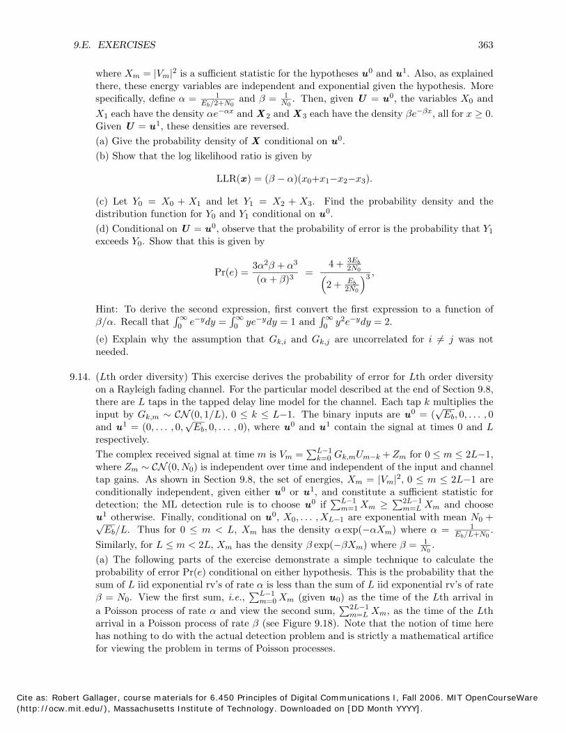
∫ ∫ ∫ �
9.E. EXERCISES 363
where Xm = |Vm|2 is a sufficient statistic for the hypotheses u0 and u1. Also, as explained there, these energy variables are independent and exponential given the hypothesis. More specifically, define α = 1 and β = 1 . Then, given U = u0, the variables X0 andEb/2+N0 N0
X1 each have the density αe−αx and X 2 and X 3 each have the density βe−βx, all for x ≥ 0. Given U = u1, these densities are reversed. (a) Give the probability density of X conditional on u0 . (b) Show that the log likelihood ratio is given by
LLR(x ) = (β − α)(x0+x1−x2−x3).
(c) Let Y0 = X0 + X1 and let Y1 = X2 + X3. Find the probability density and the distribution function for Y0 and Y1 conditional on u0 . (d) Conditional on U = u0, observe that the probability of error is the probability that Y1
exceeds Y0. Show that this is given by
3α2β + α3 4 + 3Eb
Pr(e) = (α + β)3
= ( 2N0)3 , 2 + Eb
2N0
Hint: To derive the second expression, first convert the first expression to a function of β/α. Recall that 0
∞e−ydy = 0
∞ye−ydy = 1 and 0
∞y2e−ydy = 2.
(e) Explain why the assumption that Gk,i and Gk,j are uncorrelated for i = j was not needed.
9.14. (Lth order diversity) This exercise derives the probability of error for Lth order diversity on a Rayleigh fading channel. For the particular model described at the end of Section 9.8, there are L taps in the tapped delay line model for the channel. Each tap k multiplies the input by Gk,m ∼ CN (0, 1/L), 0 ≤ k ≤ L−1. The binary inputs are u0 = (
√Eb, 0, . . . , 0
and u1 = (0, . . . , 0,√
Eb, 0, . . . , 0), where u0 and u1 contain the signal at times 0 and L respectively. ∑L−1The complex received signal at time m is Vm = k=0 Gk,mUm−k + Zm for 0 ≤ m ≤ 2L−1, where Zm ∼ CN (0, N0) is independent over time and independent of the input and channel tap gains. As shown in Section 9.8, the set of energies, Xm = |Vm|2 , 0 ≤ m ≤ 2L−1 are conditionally independent, given either u0 or u1, and constitute a sufficient statistic for detection; the ML detection rule is to choose u0 if
∑L−1 X∑2L−1 X and choose m=1 m m=L m
0 ≥
u1 otherwise. Finally, conditional on u , X0, . . . , XL−1 are exponential with mean N0 + 1
√Eb/L. Thus for 0 ≤ m < L, Xm has the density α exp(−αXm) where α = .Eb/L+N0
Similarly, for L ≤ m < 2L, Xm has the density β exp(−βXm) where β = 1 .N0
(a) The following parts of the exercise demonstrate a simple technique to calculate the probability of error Pr(e) conditional on either hypothesis. This is the probability that the sum of L iid exponential rv’s of rate α is less than the sum of L iid exponential rv’s of rate ∑L−1β = N0. View the first sum, i.e., m=0 Xm (given u0) as the time of the Lth arrival in a Poisson process of rate α and view the second sum,
∑m2L
=−L 1 Xm, as the time of the Lth
arrival in a Poisson process of rate β (see Figure 9.18). Note that the notion of time here has nothing to do with the actual detection problem and is strictly a mathematical artifice for viewing the problem in terms of Poisson processes.
Cite as: Robert Gallager, course materials for 6.450 Principles of Digital Communications I, Fall 2006. MIT OpenCourseWare (http://ocw.mit.edu/), Massachusetts Institute of Technology. Downloaded on [DD Month YYYY].
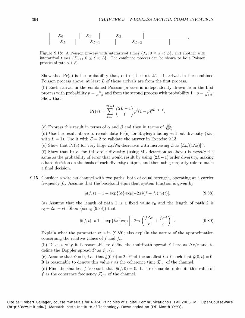
�
[ ( )]
364 CHAPTER 9. WIRELESS DIGITAL COMMUNICATION
X0 X1 X2
XL XL+1 XL+2
Figure 9.18: A Poisson process with interarrival times {Xk; 0 ≤ k < L}, and another with interarrival times {XL+�; 0 ≤ < L}. The combined process can be shown to be a Poisson process of rate α + β.
Show that Pr(e) is the probability that, out of the first 2L − 1 arrivals in the combined Poisson process above, at least L of those arrivals are from the first process. (b) Each arrival in the combined Poisson process is independently drawn from the first process with probability p = α and from the second process with probability 1−p = β .α+β α+β Show that
Pr(e) = 2∑L−1 (2L − 1
) p (1 − p)2L−1− .
=L
(c) Express this result in terms of α and β and then in terms of Eb .LN0
(d) Use the result above to re-calculate Pr(e) for Rayleigh fading without diversity (i.e., with L = 1). Use it with L = 2 to validate the answer in Exercise 9.13. (e) Show that Pr(e) for very large Eb/N0 decreases with increasing L as [Eb/(4N0)]L . (f) Show that Pr(e) for Lth order diversity (using ML detection as above) is exactly the same as the probability of error that would result by using (2L− 1) order diversity, making a hard decision on the basis of each diversity output, and then using majority rule to make a final decision.
9.15. Consider a wireless channel with two paths, both of equal strength, operating at a carrier frequency fc. Assume that the baseband equivalent system function is given by
g(f, t) = 1 + exp{iφ} exp[−2πi(f + fc) τ2(t)]. (9.88)
(a) Assume that the length of path 1 is a fixed value r0 and the length of path 2 is r0 + ∆r + vt. Show (using (9.88)) that
g(f, t) ≈ 1 + exp{iψ} exp −2πi f∆r
+ fcvt
. (9.89) c c
Explain what the parameter ψ is in (9.89); also explain the nature of the approximation concerning the relative values of f and fc. (b) Discuss why it is reasonable to define the multipath spread L here as ∆r/c and to define the Doppler spread D as fcv/c. (c) Assume that ψ = 0, i.e., that g(0, 0) = 2. Find the smallest t > 0 such that g(0, t) = 0. It is reasonable to denote this value t as the coherence time Tcoh of the channel. (d) Find the smallest f > 0 such that g(f, 0) = 0. It is reasonable to denote this value of f as the coherence frequency Fcoh of the channel.
Cite as: Robert Gallager, course materials for 6.450 Principles of Digital Communications I, Fall 2006. MIT OpenCourseWare (http://ocw.mit.edu/), Massachusetts Institute of Technology. Downloaded on [DD Month YYYY].
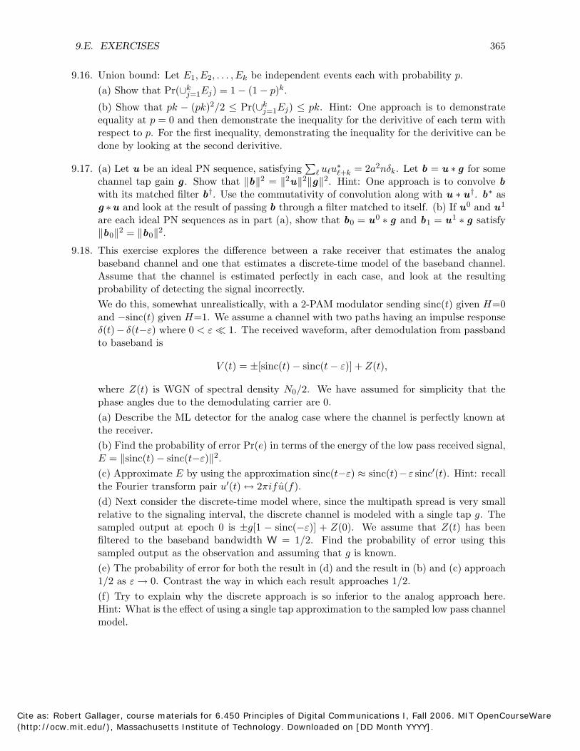
∑
9.E. EXERCISES 365
9.16. Union bound: Let E1, E2, . . . , Ek be independent events each with probability p. (a) Show that Pr(∪j
k =1Ej ) = 1 − (1 − p)k .
(b) Show that pk − (pk)2/2 ≤ Pr(∪jk =1Ej ) ≤ pk. Hint: One approach is to demonstrate
equality at p = 0 and then demonstrate the inequality for the derivitive of each term with respect to p. For the first inequality, demonstrating the inequality for the derivitive can be done by looking at the second derivitive.
9.17. (a) Let u be an ideal PN sequence, satisfying uu∗ +k = 2a2nδk. Let b = u ∗ g for some
channel tap gain g . Show that ‖b‖2 = ‖2u‖2‖g‖2 . Hint: One approach is to convolve b with its matched filter b†. Use the commutativity of convolution along with u ∗ u†. b∗ as g ∗ u and look at the result of passing b through a filter matched to itself. (b) If u0 and u1
are each ideal PN sequences as in part (a), show that b0 = u0 ∗ g and b1 = u1 ∗ g satisfy ‖b0‖2 = ‖b0‖2 .
9.18. This exercise explores the difference between a rake receiver that estimates the analog baseband channel and one that estimates a discrete-time model of the baseband channel. Assume that the channel is estimated perfectly in each case, and look at the resulting probability of detecting the signal incorrectly. We do this, somewhat unrealistically, with a 2-PAM modulator sending sinc(t) given H=0 and −sinc(t) given H=1. We assume a channel with two paths having an impulse response δ(t) − δ(t−ε) where 0 < ε � 1. The received waveform, after demodulation from passband to baseband is
V (t) = ±[sinc(t) − sinc(t − ε)] + Z(t),
where Z(t) is WGN of spectral density N0/2. We have assumed for simplicity that the phase angles due to the demodulating carrier are 0. (a) Describe the ML detector for the analog case where the channel is perfectly known at the receiver. (b) Find the probability of error Pr(e) in terms of the energy of the low pass received signal, E = ‖sinc(t) − sinc(t−ε)‖2 . (c) Approximate E by using the approximation sinc(t−ε) ≈ sinc(t)− ε sinc′(t). Hint: recall the Fourier transform pair u′(t) 2πifu(f).↔(d) Next consider the discrete-time model where, since the multipath spread is very small relative to the signaling interval, the discrete channel is modeled with a single tap g. The sampled output at epoch 0 is ±g[1 − sinc(−ε)] + Z(0). We assume that Z(t) has been filtered to the baseband bandwidth W = 1/2. Find the probability of error using this sampled output as the observation and assuming that g is known. (e) The probability of error for both the result in (d) and the result in (b) and (c) approach 1/2 as ε 0. Contrast the way in which each result approaches 1/2. →(f) Try to explain why the discrete approach is so inferior to the analog approach here. Hint: What is the effect of using a single tap approximation to the sampled low pass channel model.
Cite as: Robert Gallager, course materials for 6.450 Principles of Digital Communications I, Fall 2006. MIT OpenCourseWare (http://ocw.mit.edu/), Massachusetts Institute of Technology. Downloaded on [DD Month YYYY].