Wireless Channel Equalization in Digital Communication Systems
166
Claremont Colleges Scholarship @ Claremont CGU eses & Dissertations CGU Student Scholarship 2012 Wireless Channel Equalization in Digital Communication Systems Sammuel Jalali Claremont Graduate University is Open Access Dissertation is brought to you for free and open access by the CGU Student Scholarship at Scholarship @ Claremont. It has been accepted for inclusion in CGU eses & Dissertations by an authorized administrator of Scholarship @ Claremont. For more information, please contact [email protected]. Recommended Citation Jalali, Sammuel, "Wireless Channel Equalization in Digital Communication Systems" (2012). CGU eses & Dissertations. Paper 42. hp://scholarship.claremont.edu/cgu_etd/42 DOI: 10.5642/cguetd/42
Transcript of Wireless Channel Equalization in Digital Communication Systems

Claremont CollegesScholarship @ Claremont
CGU Theses & Dissertations CGU Student Scholarship
2012
Wireless Channel Equalization in DigitalCommunication SystemsSammuel JalaliClaremont Graduate University
This Open Access Dissertation is brought to you for free and open access by the CGU Student Scholarship at Scholarship @ Claremont. It has beenaccepted for inclusion in CGU Theses & Dissertations by an authorized administrator of Scholarship @ Claremont. For more information, pleasecontact [email protected].
Recommended CitationJalali, Sammuel, "Wireless Channel Equalization in Digital Communication Systems" (2012). CGU Theses & Dissertations. Paper 42.http://scholarship.claremont.edu/cgu_etd/42
DOI: 10.5642/cguetd/42

Wireless Channel Equalization in Digital Communication Systems
By
Sammuel Jalali
A dissertation submitted to the faculty of Claremont Graduate University and California State
University, Long Beach in partial fulfillment of the requirements for the degree of Doctor of
Philosophy in the Graduate Faculty of Engineering and Industrial Applied Mathematics
Claremont, California and Long Beach, California
2012

Wireless Channel Equalization in Digital Communication Systems
By
Sammuel Jalali
Claremont Graduate University
2012
Abstract
Our modern society has transformed to an information-demanding system, seeking voice,
video, and data in quantities that could not be imagined even a decade ago. The mobility of
communicators has added more challenges. One of the new challenges is to conceive highly reliable
and fast communication system unaffected by the problems caused in the multipath fading wireless
channels. Our quest is to remove one of the obstacles in the way of achieving ultimately fast and
reliable wireless digital communication, namely Inter-Symbol Interference (ISI), the intensity of
which makes the channel noise inconsequential.
The theoretical background for wireless channels modeling and adaptive signal processing are
covered in first two chapters of dissertation.
The approach of this thesis is not based on one methodology but several algorithms and
configurations that are proposed and examined to fight the ISI problem. There are two main
categories of channel equalization techniques, supervised (training) and blind unsupervised (blind)
modes. We have studied the application of a new and specially modified neural network requiring
very short training period for the proper channel equalization in supervised mode. The promising
performance in the graphs for this network is presented in chapter 4.
For blind modes two distinctive methodologies are presented and studied. Chapter 3 covers the
concept of multiple “cooperative” algorithms for the cases of two and three cooperative algorithms.
The “select absolutely larger equalized signal” and “majority vote” methods have been used in 2-
and 3-algoirithm systems respectively. Many of the demonstrated results are encouraging for further
research.
Chapter 5 involves the application of general concept of simulated annealing in blind mode
equalization. A limited strategy of constant annealing noise is experimented for testing the simple
algorithms used in multiple systems. Convergence to local stationary points of the cost function in
parameter space is clearly demonstrated and that justifies the use of additional noise. The capability
of the adding the random noise to release the algorithm from the local traps is established in several
cases.

v
Acknowledgement
My deep and sincere thanks to my advisor, Professor Rajendra Kumar from California State
University, Long Beach (CSULB) for his knowledgeable and kind guidance and help that I have
received in three interesting courses I took with him, and continuously since 2008 to 2012. I am also
indebted to Professor Ellis Cumberbatch from Claremont Graduate University (CGU) for his
fantastic applied mathematics courses and priceless help in the course of my education.
My especial thanks to Professor Burkhard Englert from CSULB, and Professor Allon Percus from
CGU for being encouraging dissertation committee memeber. I would like to extend my appreciation
to Professor Chit-Sang Tsang and Professor Henry Schellhorn and to the memory of Professor
Hedley Morris.

vi
Table of Contents
Acknowledgements ……………………………………………………………………………v
Table of Contents ……………………………………………………………………………..vi
Table of Figures ………………………………………………………………………………viii
Thesis Outlook ………………………………………………………………………………. 1a
Chapter 1: Wireless Channel Models and Diversity Techniques
1.1 Introduction …………………………………………………………………….…………. 1
1.2 Large Scale Fading or Attenuation ………………………………………..…………….… 2
1.3 Small Scale Fading ……………………………………………………..……………….… 4
1.4 Frequency Dispersion Parameters ………………………………………………………… 9
1.5 Wireless Channel Models ………………………………………………………………… 13
1.6 Inter-Symbol-Interface Cancellation and Diversity …………………………….………… 18
1.7 References ………………………………………………………………………………… 24
Chapter 2: Adaptive Algorithms and Channel Equalization
2.1 Introduction ………………………………………………………………………..……… 26
2.2 Channel Equalization ……………………………………………………………………… 29
2.3 Deconvolution of A-Priori Known Systems ……………………………………………… 34
2.4 Adaptive Algorithm for Equalization of A Priori-Unknown Channels …………………… 36
2.5 Blind Equalization Algorithms ………………………………………………….………… 37
2.6 Bussgang Algorithms ……………………………………………………………………… 41
2.7 References ……………………………………………………………………………….… 50
Chapter 3: Blind Channel Equalization using Diversified Algorithms
3.1 Introduction ………………………………………………………………………….…… 53
3.2 Recursive Least Squares Adaptive Algorithms …………………………………...……… 54
3.3 General Cooperative Adaptive System with Diversified Algorithm……………………… 58
3.4 Adaptive Systems with Two Algorithms …………………….…………………………… 63
3.5 Adaptive Systems with Three Algorithms …………………...…………………………… 72
3.6 Chapter Conclusion …………………………………..…………………………………… 86
3.7 References ………………………………………………………………………………… 88
Chapter 4: Neural Networks, a Novel Back Propagation Configuration for Wireless Channel
Equalization
4.1 Introduction ……………………………………………………………..………………… 89
4.2 Fundamental Theory of Neural Networks ………………………………………………… 92
4.3 Network Architectures and Algorithms …………………………………………………… 95
4.4 A Novel Neural Network as Wireless Channel Equalizer ………………………………… 98
4.5 Learning Algorithm ………………………………….…………………………………… 103
4.6 Performance and Simulation Results for the Proposed Network ………………………… 109

vii
4.7 Convergence Analysis …………………………………………………….……………… 119
4.7 References ………………………………………………………………………………… 126
Chapter 5: Adaptive Simulated Annealing
5.1 Introduction ……………………………………………………………..……………….. 130
5.2 Adaptive Simulated Annealing in Channel Equalization ……………………………...… 133
5.3 Simulation Results on Different Channels ………………………………………….…… 135
5.4 Chapter Conclusion …………………………………………………………………..….. 145
5.5 References ……………………………………………………………………………...… 147
Appendix A ………………………………………………………………………………..…. 149
Chapter 6: Concluding Remarks and the Future Research …………………………………... 152

viii
List of Figures
1-1 Multipath channel in wireless communications ……………………………………………1
1-2 Example of two-ray geometry …………………………………………………………… 5
1-3 Channel modeling by Channel Impulse Response (CIR) ………………………………..... 5
1-4 An ideal Channel Impulse Response (CIR) ………………………………………………. 6
1-5 Doppler shift geometry ………………………………………………………………….... 9
1-6 Example of the channel time-variation computing ………………………………………..12
1-7 Simple wireless channel model …………………………………………………………... 13
1-8 Basic diversity combination methods …………………………………………………….. 21
1-9 Hybrid diversity combination method …………………………………………………… 22
1-10 MIMO system basic configuration ……………………………………………………… 23
2-1 Continuous time channel method ………………………………………………………… 30
2-2 Discrete-time model of channel ………………………………………………………….. 31
2-3 General diagram of supervised equalization system ……………………………………… 36
2-4 Bussgang Theorem ……………………………………………………………………….. 37
2-5 Basic linear equalization system ………………………………………………………….. 38
2-6 Basic equalization system ………………………………………………………….…….... 41
2-7 Basic Decision Feedback Equalizer diagram ……………………………………………... 46
3-1 Blind equalizer system with diversified algorithms …………………………………… … 53
3-2 General Recursive Least Squares algorithm ………………………………………………. 54
3-3 The improvement of the probability of correct estimate in 3-algorithm equalizer ……….. 59
3-4 The degradation of the probability of correct estimate in 4-algorithm equalizer ………… 60
3-5 The improvement of the probability of correct estimate in 5-algorithm equalizer ……….. 61
3-6 The configuration for cooperative 2-algorithm equalizer system ………………………… 62
3-7 Independent residual ISI of LMS (top) and EWRLS (bottom) algorithms ………………. 64
3-8 Cooperative residual ISI of LMS (top) and EWRLS (bottom) algorithms ………………. 65
3-9 Comparison of LMS algorithm residual ISI for independent (magenta) and cooperative (blue)
modes ……………………………………………………………………………………... 66
3-10 Comparison of EWRLS algorithm residual ISI for independent (magenta) and cooperative
(blue) modes ……………………………………………………………………………… 66
3-11 Independent residual ISI of LMS (top) and EWRLS (bottom) algorithms …………….. 68
3-12 Cooperative residual ISI of LMS (top) and EWRLS (bottom) algorithms ……………. 69
3-13 Comparison of LMS algorithm residual ISI for independent (magenta) and cooperative (blue)
modes ……………………………………………………………………………………... 70
3-14 Comparison of EWRLS algorithm residual ISI for independent (magenta) and cooperative
(blue) modes …………………………………………………………………………….… 70
3-15 The configuration for cooperative 3-algorithm equalizer system …………………….…. 71
3-16 Independent residual ISI of LMS (top), EWRLS (middle), and QS-2 (bottom) algorithms
………………………………………………………………………………………………73
3-17 Cooperative residual ISI of LMS (top), EWRLS (middle), and QS-2 (bottom) algorithms
………………………………………………………………………………………………74
3-18 Comparison of LMS algorithm residual ISI for independent mode (red) and cooperative mode
(blue) ………………………………………………………………………………………… 75
3-19 Independent residual ISI of LMS (top), EWRLS (middle), and QS-2 (bottom) algorithms ..77
3-20 Cooperative residual ISI of LMS (top), EWRLS (middle), and QS-2 (bottom) algorithms ..78
ix
3-21 Comparison of LMS algorithm residual ISI for independent mode (red) and cooperative mode
(blue) ………………………………………………………………………………………… 79
3-22 Comparison of RLS algorithm residual ISI for independent mode (red) and cooperative mode
(blue) ………………………………………………………………………………………… 80
Figure 3-23 Independent residual ISI of LMS (top), EWRLS (middle), and QS-2 (bottom)
algorithms ……………………………………………………………………………………. 82
3-24 Cooperative residual ISI of LMS (top), EWRLS (middle), and QS-2 (bottom) algorithms ..83
3-25 Comparison of LMS algorithm residual ISI for independent mode (red) and cooperative mode
(blue) …………………………………………………………………………………………. 84
3-26 Comparison of RLS algorithm residual ISI for independent mode (red) and cooperative mode
(blue) …………………………………………………………………………………………. 84
3-27 Comparison of QS-2 algorithm residual ISI for independent mode (red) and cooperative mode
(blue) …………………………………………………………………………………………. 85
4-1 Basic perceptron architecture ……………………………………………………………….. 90
4-2 The perceptron architecture with general nonlinear activation function ………………….... 93
4-3 A multilayer perceptron example of two layer model with N neurons in the input and M neurons
in the output layer …………………………………………………………………………… 96
4-4 Proposed neural network equalizer architecture ………………………………………….... 100
4-5 Detailed block diagram of the proposed neural network based adaptive equalizer ……...… 101
4-6 Instantaneous error (top) and the bit errors that have occurred during the adaptation process
(bottom) ….……………………………………………………………………………….. 110
4-7 Mean Square Error (MSE) averaged over a moving window of 50 steps ………………... 111
4-8 Instantaneous error (top) and the only bit errors that have occurred during the adaptation process
(bottom) ………………………………………………………………………………….… 112
4-9 Mean Square Error (MSE) averaged over a moving window of 50 steps ………………….. 112
4-10 Instantaneous error (top) and the bit errors for the case without the delay adjustments (bottom).
……………………………………………………………………………………………… 113
4-11 Mean Square Error (MSE) without the delay adjustments ………………………………. 114
4-12 Instantaneous error (top) and the bit errors (bottom) for the case without the delay adjustments
after increasing the training period from 40 to 100 steps. …………………………………. 114
4-13 Instantaneous error (top) and the only bit errors that have occurred during the adaptation
process (bottom) …………………………………………………………………………… 116
4-14 Mean Square Error (MSE) averaged over a moving window of 50 steps ……………….. 117
4-15 Instantaneous error (top) and the data errors (bottom) versus iteration number k ……….. 117
4-16 A simplified and low-dimensional example of two-layer network ……………………… 119
4-17 A graph of hyperbolic tangent function ………………………………………………….. 123
5-1 The decision-directed system configuration to include random noise application ………… 131
5-2 The alternative system configuration to include additional random noise ………………… 133
5-3 Comparison of residual ISI for the case of EWRLS ……………………………………….. 135
5-4 Comparison of residual ISI for the case of EWRLS ……………………………………….. 136
5-5 Comparison of final equalizer convolution with the CIR ………………………………….. 137
5-6 Comparison of residual ISI for the case of EWRLS ……………………………………….. 138
5-7 Comparison of final equalizer convolution with the CIR…………………………………… 139
5-8 Comparison of residual ISI for the case of EWRLS …………………………………..…… 140
5-9 Comparison of final equalizer convolution with the CIR ………………………………..… 141
5-10 Comparison of residual ISI for the case of EWRLS ……………………………………....142
5-11 Comparison of final equalizer convolution with the CIR ……………………………….... 143

x
5-12 Comparison of residual ISI for the case of EWRLS ………………………………………..144
5-13 Comparison of residual ISI for the case of EWRLS ……………………………………..…145

1a
Thesis Outlook
Our modern society has transformed to an information-demanding system, seeking voice,
video, and data in quantities that could not be imagined even a decade ago. Mobility of
communicators has added new challenges in the path to accomplish the goal of providing all the
information asked for in any possible location. One of the new challenges is to conceive highly
reliable and fast communication system unaffected by the problems caused in the multipath fading
wireless channel.
Our quest in this thesis is to help remove one of the obstacles in the way of achieving ultimately fast
and reliable wireless digital communication, namely Inter-Symbol Interference (ISI), the severity of
which makes the channel noise inconsequential.
An introduction to wireless channel characteristics and modeling is given in chapter one. This
includes the large scale and small scale fading phenomena in section 1.2 and 1.3 respectively, and
the mathematical models for wireless channels in section 1.5. An emerging ISI cancellation
technique by space diversity is also discussed in the last section of chapter one.
Since most of the techniques used to achieve the aforementioned goal are adaptive in nature, chapter
two is dedicated to a review of the main adaptive algorithms as well as some other methods to invert
a-priori known channels. The deconvolution technique for inverting known channels (by their
approximate impulse response) is discussed in section 2.3; when other techniques for the known
channel are given in section 2.4. Blind equalization techniques with relatively low computational
cost are discussed in section 2.5. A major family of these techniques that are collectively called
Bussgang algorithms are reviewed in the concluding section of chapter 2.
Our contributions are mainly in chapter 3 and 4. A new methodology to approach the blind
equalization which was mentioned in the research proposal by using diverse algorithms is treated in
chapter 3. First a few more algorithms with relatively simple computations that are being

1b
incorporated in diversified systems in chapter 3 are given in section 3.2. These include RLS,
EWRLS, and Quantized State recursive methods. In section 3.3 the general idea of cooperation of
two or more algorithms is discussed and with some very optimistic expectations the effectiveness of
them are shown. Section 3.4 introduces the configuration that uses two algorithms with
corresponding simulation results, while the main idea of majority vote among the algorithms
contributing to the systems with 3 simultaneous ones is given in section 3.5. The latter section
includes the important simulation results for the system of three that is the pinnacle of this chapter.
Chapter 3 concludes with a brief summary of the results.
An alternative to blind methods that can use a very short training period seems attractive in practice.
Especially if the proposed method is simple in architecture, it can be employed to replace the less
reliable blind equalization techniques. After an introduction, and the review of the fundamental
theory of neural networks in sections 4.1 and 4.2 the well-known back propagation algorithm for
neural networks is presented in section 4.3. The application of the proposed architecture to the
problem of wireless channel equalization is formulated in section 4.4. The learning algorithm details
for the proposed network are summarized in section 4.5. The performance and the simulation results
are included in section 4.6 of this chapter. A weak convergence analysis of the output layer is
discussed in section 4.7 (this is different from the well-known Rosenblatt perceptron convergence
that does not include any activation function, such as the hyperbolic tangent blocks in our proposed
network). While the input layer convergence analysis seems out of reach at present, it is left to the
future research.
Another concept that was originally intended to be developed also for blind mode systems as a
promising methodology is approached in chapter 5 under the Adaptive Simulated Annealing
terminology. After an introduction to the elements of simulated annealing and a short history of its
application are given in section 5.2, in section 5.3 we argue that this technique should facilitate the
convergence, at least in theory. Some preliminary results are shown in the following section.

1c
Finally chapter 6 presents an overall collective summary of the results obtained in this thesis and
delineates the path for future continuation of related research by the author and the research
community, in particular in the field of adaptive signal processing.

1
Chapter 1: Wireless Channel Models and Diversity techniques
1.1 Introduction
Wireless communication has gone through major changes in the last few decades. While it
mostly had been used for satellite, terrestrial links and broadcasting until the 1970s, cellular and
wireless networking and other Personal Communication Systems (PCS) presently dominate the
technology of modern wireless communications.
The generally used Additive White Gaussian Noise (AWGN) model does not adequately represent
the channel for these modern applications. Moreover, the Line-Of-Sight (LOS) path between the
transmitter and the receiver may or may not exist in such a channel.
An important characteristic of the wireless channel is the presence of many different paths between
the transmitter and the receiver (See Figure 1-1).
* Reflection
* Scattering
* Diffraction
Figure 1-1 Multipath channel in wireless communications.
Basic Electromagnetic (EM) wave propagation phenomena such as scattering that occurs along these
paths further increases the number of the paths between the communicators.

2
Common propagation phenomena encountered are:
1. Reflection: EM waves are reflected when impinging on objects in their paths if the physical
size of the objects are much greater than the wavelength of the EM waes.
2. Diffraction: Characterized as the sharp changes in the propagation path of EM waves that
occur when they hit an obstacle with surface irregularities such as sharp edges.
3. Scattering: Occurs when EM waves visit a cluster of objects smaller in size than the
wavelength, such as water vapor and foliage. Scattering causes many copies of the EM wave
to propagate in different directions.
There are other infrequent phenomena such as absorption and refraction that might take place in
common wireless channels.
The signal power is the critical parameter in a communication channel. The power reducing effects
have been studied in two major cases:
1. Large-scale effect characterizes the signal power usually with respect to long propagation
distances and results in the mean path loss of the signal.
2. Small-scale effect or fading concerns the relatively fast changes in the signal amplitude and
its power. It characterizes the signal power fluctuations over short distance and time
intervals around the mean signal power.
1.2 Large Scale Fading or Attenuation
In general, the average power of the received signal decreases logarithmically with the
distance between the transmitter and the receiver. The attenuation caused by the distance is called
large scale effect or path loss. The propagation medium and the environment would also have some
effect on the total loss of the signal strength.
3
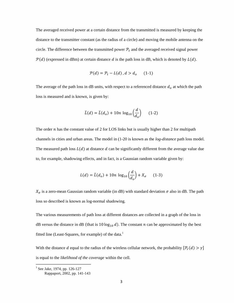
The averaged received power at a certain distance from the transmitted is measured by keeping the
distance to the transmitter constant (as the radius of a circle) and moving the mobile antenna on the
circle. The difference between the transmitted power and the averaged received signal power
( ) (expressed in dBm) at certain distance is the path loss in dB, which is denoted by ( ).
( ) ( ) ( )
The average of the path loss in dB units, with respect to a referenced distance at which the path
loss is measured and is known, is given by:
( ) ( ) (
) ( )
The order has the constant value of 2 for LOS links but is usually higher than 2 for multipath
channels in cities and urban areas. The model in (1-20 is known as the log-distance path loss model.
The measured path loss ( ) at distance can be significantly different from the average value due
to, for example, shadowing effects, and in fact, is a Gaussian random variable given by:
( ) ( ) (
) ( )
is a zero-mean Gaussian random variable (in dB) with standard deviation also in dB. The path
loss so described is known as log-normal shadowing.
The various measurements of path loss at different distances are collected in a graph of the loss in
dB versus the distance in dB ( ). The constant can be approximated by the best
fitted line (Least-Squares, for example) of the data.1
With the distance equal to the radius of the wireless cellular network, the probability [ ( ) ]
is equal to the likelihood of the coverage within the cell.
1 See Jake, 1974, pp. 126-127
Rappaport, 2002, pp. 141-143

4
The percentage of coverage area (that is, the fraction of the area within the cell that will have an
acceptable power level) is:
( )
∫ ∫ [ ( ) ] ( )
This percentage may be computed in terms of the error function erf as follows(see [6] and [7]):
( )
( ( ) (
) [ (
)]) ( )
( )
√
√ ( )
√ ∫
When the signal level is ( ) (that is ), then:
( )
[ (
) ( (
))] ( )
1.3 Small Scale Fading
Due to multipath propagation, more than one version of the transmitted signal arrive at the
mobile receiver at slightly different times. The interference induced by these multiple copies, also
known as multipath waves, has become the most significant cause of distortion known as fading and
Inter-Symbol Interference (ISI). The radio signal experiences rapid changes of its amplitude over a
relatively short period of time (See Figure 1-2).
The waves travelling different paths, therefore travelling different distances, sum up at the receiver
antenna (or antenna array in some cases) to generate ISI of such a magnitude that the effects of large-
scale path loss can be completely ignored by comparison.

5
d1
d2
d0θ
θ
Rx
Tx
Figure 1-2 Example of two-ray geometry
There are a variety of ways to statistically model the wireless channels in order to represent the
random behavior of multipath fading. One simple and popular model represents the fading channel
with a linear and time-varying Channel Impulse Response (CIR) denoted by the function ( )
s (t) r (t)h (t,τ)
Figure 1-3 Channel modeling by Channel Impulse Response (CIR)
Time Dispersion Parameters
A perfect channel from a communications point of view is one that has a constant gain and a
linear phase response, or at least possesses these features over a desired frequency range or
bandwidth.

6
Such a frequency range should be larger than the frequency spectrum of the transmitted signal to
preserve the signal spectral characteristics. Consequently, such an ideal channel can be symbolically
shown as ( ) ( ) (See Figure 1-4), with as a constant.
goδ(t)
τ0t
Figure 1-4 An ideal Channel Impulse Response (CIR)
Such channel impulse response implies only one received signal (delayed by ), causing no ISI even
when the gain varies with time as the varying CIR of ( ) ( ) ( ) where ( ) is relatively
slowly varying function of time and in general may be complex valued. If we assume that the
multipath channel includes different paths, and let the power and delay of path be given by
respectively, then the weighted average delay (also known as mean excess delay) is
defined as:
∑
∑
( )
The second statistical moment of the delay may also be computed by:
∑
∑
( )
The channel delay spread, that is the rms value of the delay, is given by:
√ ( ) ( )

7
The channels with time-dependent response (CIR) given by ( ) will have time-dependent
frequency response ( ) (In fact, as will be stressed later, the CIRs change very slowly with
respect to time in most practical cases) with
( ) ∫ ( )
( )
To determine the wireless channel characteristics in the frequency domain, first we need to
determine the correlation coefficient or factor of the channel frequency response, based on a change
in frequency of the size or .
( ) { ( ) ( )}
{ ( ) ( )} { ( ) ( )}
{| ( )| }
∫ | ( )|
∫ | ( )|
( )
The coherence bandwidth is the counterpart of the delay spread in the frequency domain, and it is the
range of frequencies over which the channel gain remains about the same, or as is commonly known,
over the range of frequencies the gain is flat, with a linear phase. Fortunately, the coherence
bandwidth of the channel denoted by can be approximated based on the specified correlation
coefficient value.
The case when the correlation coefficient is about zero, ( ) . The coherence
bandwidth for this case is approximated by , which implies that changing the frequency by
results in a completely different (and statistically independent) gain.
For the more common value of ( ) ( ),the coherence bandwidth is estimated by
, which implies that the channel gain at and are similar.

8
Finally, when considering ( ) ( ), the coherence bandwidth can be approximated as
. In this case, the channel gain at is almost exactly the same as the gain at .
Based on the value of coherence bandwidth , and given signal bandwidth , one can evaluate the
channel category. When , the channel is considered flat or flat fading.
Denoting the symbol time duration by then the minimum signal bandwidth can be estimated as
. This signal bandwidth therefore has to be quite a bit less than the channel coherence
bandwidth so that the channel can be assumed to be flat fading. A rule of thumb is given by
In the case of a flat fading channel, no compensation for the channel distortion is required.
Consequently, the symbol rate in the channel has an upper bound
.
When the above condition is not met, that is, the ISI exists and the received signal is
distorted.
In most common multipath channels the ISI distortion effects are significant and dominate the
channel noise. Such channels are said to be highly dispersive, and engineering efforts are focused on
eliminating ISI by a process known as equalization in communication discipline, or de-convolution
in some other applications such as geophysics.
In conclusion, we divide the channel behavior with respect to the signal bandwidth and according to
the channel delay spread as follows:
When and the channel is known as flat fading or frequency-not-selective.
When and the channel is known as non-flat or frequency-selective.

9
1.4 Frequency Dispersion Parameters
The mobility of the communicator originates another parameter known as Doppler shift in
frequency, or simply some change in frequency due to the mobile velocity.
When denoted by , the Doppler shift is computed as
, in which is the relative mobile
speed, is the radio wavelength, and is the angle between the wave direction and the mobile
direction. The change in frequency is positive when the mobile approaches the transmitter and
negative when the mobile is departing.
Radio
Wave
θ
v
Figure 1-5 Doppler shift geometry
It is obvious that different paths have different Doppler shifts that possess random natures, as the
angle can be considered random and in most cases uniformly distributed.
There are a number of copies of the transmitted waves at the mobile antenna, each travelling along
different paths, which are characterized by various relative speeds and angles. Moreover, in specific
scenarios, the surrounding objects might be moving and generating time varying Doppler shifts on
multiple components.
The corresponding random change in frequency causes spectral broadening known as Doppler
spread. Doppler spread is therefore defined as the range of frequencies over which the Doppler shift
10
is not zero. We denote by the maximum Doppler shift or Doppler spread of a specific wireless
channel.
It is possible to categorize the wireless channel with respect to Doppler spread as follows:
If the signal bandwidth is much greater than Doppler spread, that is , the fading is
known as slow fading and, hence, the effects of Doppler spread are negligible. In this case,
the channel (in particular, CIR) changes at a much slower rate and can be assumed to be
static over several symbol time durations.
If, on the contrary, the effects of the Doppler spread are significant and cannot be ignored in
the case that , the CIR changes rapidly with respect to the symbol time duration.
Such channel is called fast fading.
The time domain properties of the wireless channel can be further specified by defining another
parameter, coherence time, which is the duration of time in which the CIR is invariant. Two samples
of the channel are highly correlated if their time separation is less than the coherence time. The
given definition itself depends on the time correlation coefficient.
The correlation coefficient in the time domain as a function of time difference is given by:
( ) { ( ) ( )}
{| ( )| }
Generally, the coherence time is inversely proportional to the Doppler spread.
If the coherence time for which the time correlation coefficient of Equation (1-12) remains above
or it is approximated by:

11
As a rule of thumb, the geometric average of 1-13 and 1-14 is used for digital communication.
√
( )
The channel characteristics can be categorized using the coherence time , and the symbol time
duration as follows:
When , the complete signal or symbol is affected similarly by the channel, and the
channel is known as slow fading.
When , different parts of a signal are affected differently because the channel
changes faster compared to a symbol duration. Consequently, the channel is called fast
fading.
In summary, wireless channels can be divided into four types. Based on the delay spread, the channel
is either flat (not frequency selective) or frequency selective, and based on Doppler spread (or,
equivalently, coherence time) the channel is known as slow or fast fading.
As we will see, commonly encountered wireless channels in modern mobile communication systems
are determined to be selective and slow fading. That is, the channels are usually highly dispersive.
However, the variation of channels is slow with respect to time.
To investigate the time variation of typical wireless channels, consider the scenario of Figure 1-6 in
which the mobile is travelling at 50 mph (approximately 23 m/s) at an angle of 40° to the cardinal
East-West direction.

12
d2
d1
d0θ
θ
MS
BS
φ = 40o
v
Figure 1-6 Example of the channel time-variation computing
The path length for the ray shown in the figure is computed by √ ( )
in meters
and the corresponding delay in seconds by
. Given the geometric distances:
, the delay . If we assume a symbol rate of
ksps that is equivalent of symbol time the time delays after 10,000 symbols (
s) is computed as . That is a change of less than in the time delay of the
travelling ray. This example justifies the assumption that time variation of the wireless channels are
significantly slow in comparison to common symbol rates (we have used a worst case scenario here.)
13
1.5 Wireless Channel Models
Analytical modeling of wireless channel variations and the evaluation of their effects on
transmitted signals is essential for capacity and coverage optimization including radio resource
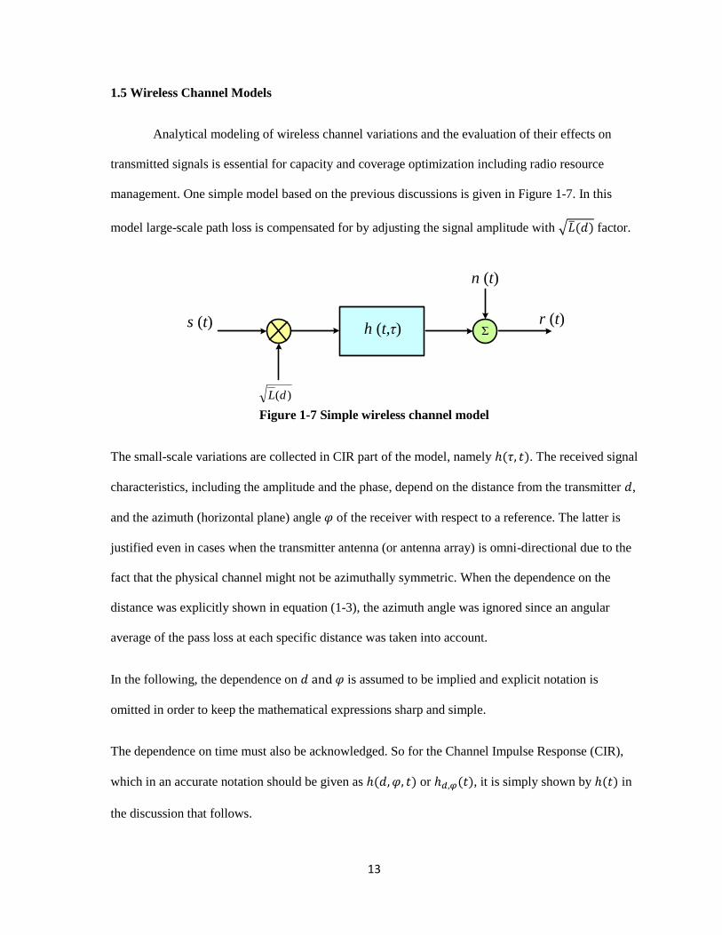
management. One simple model based on the previous discussions is given in Figure 1-7. In this
model large-scale path loss is compensated for by adjusting the signal amplitude with √ ( ) factor.
s (t) r (t)h (t,τ)
)(dL
Σ
n (t)
Figure 1-7 Simple wireless channel model
The small-scale variations are collected in CIR part of the model, namely ( ). The received signal
characteristics, including the amplitude and the phase, depend on the distance from the transmitter ,
and the azimuth (horizontal plane) angle of the receiver with respect to a reference. The latter is
justified even in cases when the transmitter antenna (or antenna array) is omni-directional due to the
fact that the physical channel might not be azimuthally symmetric. When the dependence on the
distance was explicitly shown in equation (1-3), the azimuth angle was ignored since an angular
average of the pass loss at each specific distance was taken into account.
In the following, the dependence on is assumed to be implied and explicit notation is
omitted in order to keep the mathematical expressions sharp and simple.
The dependence on time must also be acknowledged. So for the Channel Impulse Response (CIR),
which in an accurate notation should be given as ( ) or ( ), it is simply shown by ( ) in
the discussion that follows.
14
The channel model of a linear time-varying impulse response is approximated by one or multiple
delta functions for the flat-fading or frequency-selective cases respectively. The delta functions have
variable and generally complex-valued amplitudes that need to be statistically modeled.
In the first case we assume that no Line-Of-Sight (LOS) path between the transmitter and the
receiver exist. Considering available paths in the channel, the received signal comprises a
collection of weighted and delayed signals (in terms of an unmodulated sinusoidal carrier
signal) and an independent random noise process:
( ) ∑
( ) ( ) ( )
( ) ( )∑ ( )
( )∑
( ) ( )
( ) ( ) ( ) ( ) ( ) ( )
By using the central-limit-theorem and fair assumptions about the physical environment,
( ) ( ) parameters are estimated as iid (identical and independently distributed) zero-
mean Gaussian random variables with their variance noted by .
The envelope ( ) √ ( ) ( ) is distributed according to Rayleigh pdf (probability
distribution function) and is usually independent of time.
( )
(
) ( )
The phase component is:
( ) ( ( )
( )) ( )

15
The phase variable is commonly accepted to be uniformly distributed in [– ] follows
from iid assumption. The average power of the received signal can be evaluated as [ ]
[ ] [ ]
The small-scale variations of the channel as collected in the CIR, ( ) is modeled with
one or multiple delta functions adjusted by a complex-valued path gain. The CIR is
simplified and given by:
( ) ∑ ( )
( ) ( )
The CIR equation reduces a single delta function in flat-fading channels as
Moreover, the path gains are assumed to be time-independent (in fact, slowly varying with
time), when the phase components ( ) may change rapidly in time. Their distributions
have already been given in (1-19) and (1-20) for respectively. The received
baseband signal is usually normalized so that ∑
. When the channel is frequency-
selective, all but one of the components in (1-20) are undesired and interfere with the main
desired component. The desired component is specified by ( ). The important measure
of the quality of ISI-elimination is known as residual ISI computed in dB:
(∑
) (
) ( )
The last term in Equation (1-21) is valid when the signal power is normalized.
The power-delay profile of multipath channels is defined by the square of the magnitude of
path gains as a collection of delta or impulse functions ∑ ( )
.

16
The second case of modeling path gains includes a dominant approximately stationary LOS
component in addition to random multipath components. In this case the path gain
( ) ( ) are no longer zero-mean, nonetheless they are Gaussian with equal variance.
Let [ ] and [ ] with equal variance noted by . We define √
as a non-centrality parameter, and
as the Rice factor. The pdf of the
envelope √ will be Ricean as follows:
( )
(
) (
) ( )
The ( ) part is the modified Bessel function of the 0th order. This function, in closed form,
can be written:
( )
∫ ( )
∫ ( )
( )
It is computed using series expansions with ( ) (see for example, Jeffery 2005 or
Abramowitz and Stegun 1964).
Obviously, when the LOS disappears, the non-centrality and the pdf converges to
Rayleigh.
Finally, for urban zones and cities with closely spaced buildings where no dominant LOS or
specular component exists, the small-scale multipath channel is more accurately modeled by
the Nakagami distribution, which models the magnitude of the path gains relatively better as
compared to the Rayleigh distribution.
Considering [ ] ( ) and defining
[( ) ] , the Nakagami pdf is given as:

17
( )
( )(
)
(
) ( )
When ( ) ∫ ( )
is Gamma function with ( )
The Nakagami distribution is equivalent to the well-known Gamma distribution with
parameters
and if we substitute random variable with as in the
following pdf:
( )
( ) (
) ( )
Furthermore, the Nakagami reduces to the Rayleigh distribution when .
In concluding this section, we need to stress some important issues in the discussion presented
above.
a. As was mentioned, the two components of the channel path gains ( ) ( ) are
independent and can be dealt with separately. In some cases, the envelope √ is
assumed to be relatively constant in time (slowly varying) and the phase (
) may
be constant and ignored as it is tracked by the receiver. Such assumptions approximate the
channel with a real impulse response.
b. In digital communication, the baseband signals (received signal), after processing with
matched filter and the sample and hold circuit are represented by a discrete-time impulse
response or equivalently by a transversal filter of finite length. Such CIR is written by the
sequence { [ ]} , and in terms of unit impulses by ∑ [ ] [ ]
when the CIR is
approximated by a finite-length sequence of size In general, the components { [ ]} can be
complex or real-valued.

18
c. When the channel model is closer to a recursive filter representation, it can still be adequately
modeled with an infinite, or more practically with a very large transversal filter.
1.6 Inter-Symbol-Interface Cancellation and Diversity
Highly dispersive channels require some advanced processes to reduce, and possibly eliminate
the ISI effects. In practice, these channels are approximately invariant during the time that the
necessary process is executed. Moreover, some means of adaptation to compensate and adjust for
the slow variations of the channel must be applied.
a. The first of the algorithms introduced here can be one among various approaches employed
to eliminate ISI in general. These techniques are all designed to nullify or at least mitigate
the effect of the channel response. This group is known to perform channel equalization.
When employing a training period the channel equalization has the form of a straightforward
and relatively simple adaptive system. It is the blind equalization (no training period) that
has generated a great amount of literature with regard to relevant research. Unsupervised
(blind) channel equalization problems have been solved by many different approaches each
employing different and possible-to-estimate channel characteristics.
b. The Orthogonal Frequency Division Multiplexing (OFDM) Technique can be considered an
independent solution to ISI problems. Although the channel equalization should also be
performed in OFDM systems, it should be noted that the channels seem to be different by
having narrow frequency band in OFDM systems. In particular, they reduce to flat-fading or
frequency nonselective as the signal is segmented into many component ……..
c. The performance measures, such as the probability of error in fading channels, can be
improved by transmitting the same information through more than one (possibly many)

19
independent channels. The techniques exploiting this idea are known as diversity techniques,
and the information copies can be obtained in time, space, or frequency.
Modern digital communication systems incorporating diversity techniques are collectively MIMO
(Multiple Input Multiple Output) systems. These systems can also have multiple inputs but single
output (MISO), or only multiple outputs with single input (SIMO).
One diversity gain has been defined by [1]:
( )
( ) ( )
Where is the probability of bit error or Bit Error Rate (BER) and is the Signal-to-Noise Ratio
(SNR) entered in log-scale into the equation.
MIMO systems should offer answers to two essential questions: how to create diversity (in time,
space and frequency) and how to use the diversity to achieve the highest performance via reduction
in the probability of error.
The diversity can be gained by creating independently fading channels separated in time, frequency,
or space as follows:
a. Using different carrier frequencies when frequency separation must be much greater than
coherence bandwidth (
).
b. Using different time slots (temporal diversity) when the separation must be greater than
coherence time (
).
20
c. Using different antennas (spatial diversity) when the spatial separation of the transmitter or
the receiver antennas must be at least equal to or more than the half-wavelength of the
carrier frequency (
) .
It must be mentioned that exploiting temporal diversity is possible only when the mobile is in
motion, otherwise when the mobile is stationary (the moving objects surrounding the receiver can
also create Doppler shift), the Doppler shift is zero, and creating independent channels in time is
consequently not feasible.
Furthermore, polarization diversity, including vertical or horizontal polarization is not seriously
accepted or considered, perhaps because it can only provide a diversity of order two.
The second question seeks some invention of a method to take advantage of the existing diversity in
an efficient way. To see how this has been achieved in what appears to be the classic literature (See
Jake 1974), we first consider the cases with multiple antennas at the receiver only, collectively called
SIMO (Single-Input-Multiple-Output). We will include a short introduction to the cases containing
multiple transmitter antennas also to visit MIMO systems.
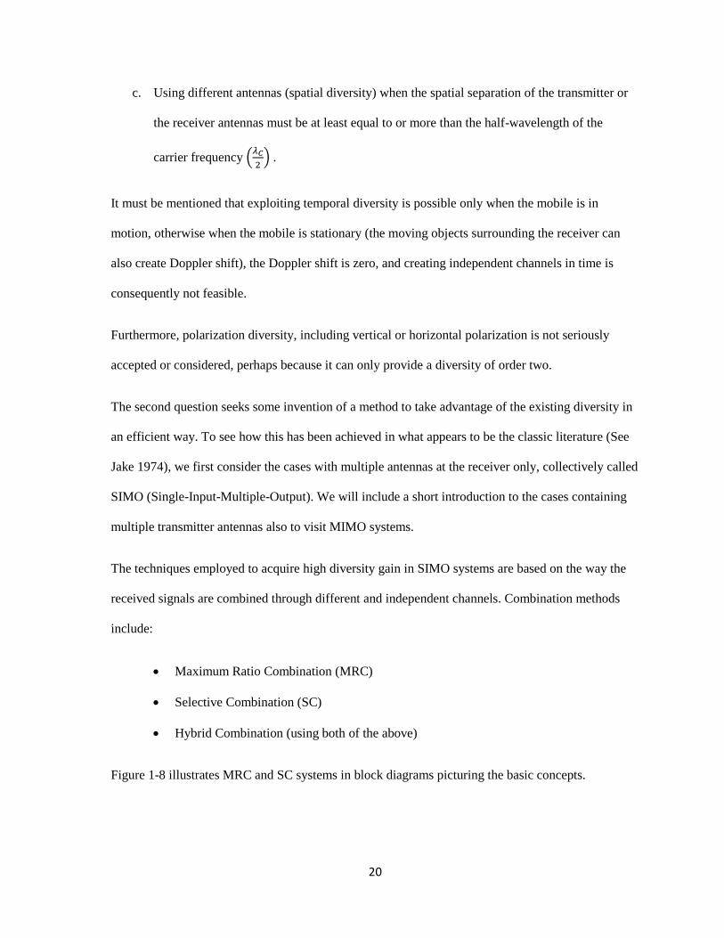
The techniques employed to acquire high diversity gain in SIMO systems are based on the way the
received signals are combined through different and independent channels. Combination methods
include:
Maximum Ratio Combination (MRC)
Selective Combination (SC)
Hybrid Combination (using both of the above)
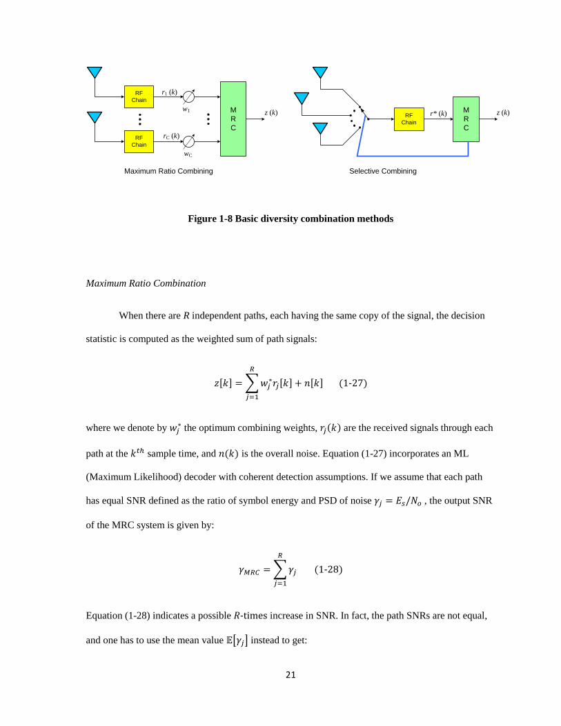
Figure 1-8 illustrates MRC and SC systems in block diagrams picturing the basic concepts.
21
RF
Chain
RF
Chain
M
R
C
r1 (k)
rC (k)
w1
wC
z (k) RF
Chain
M
R
C
r* (k) z (k)
Maximum Ratio Combining Selective Combining
Figure 1-8 Basic diversity combination methods
Maximum Ratio Combination
When there are R independent paths, each having the same copy of the signal, the decision
statistic is computed as the weighted sum of path signals:
[ ] ∑ [ ]
[ ] ( )
where we denote by the optimum combining weights, ( ) are the received signals through each
path at the sample time, and ( ) is the overall noise. Equation (1-27) incorporates an ML
(Maximum Likelihood) decoder with coherent detection assumptions. If we assume that each path
has equal SNR defined as the ratio of symbol energy and PSD of noise , the output SNR
of the MRC system is given by:
∑
( )
Equation (1-28) indicates a possible - increase in SNR. In fact, the path SNRs are not equal,
and one has to use the mean value [ ] instead to get:

22
[ ] ( )
Selective Combination
MRC systems demand significant hardware for many Radio RF chains; SC is the design
based on one single radio that picks the best received signal with respect to SNR of the channels. The
selection can be realized, for example, by choosing one of the receiver antennas as the most efficient
one. The diversity gain measured by SNR of the output signal has been determined, assuming
Rayleigh fading and keeping other regular assumptions applied in derivation of Equation (1-29).
The average SNR in SC systems is computed as:
[ ]∑
( )
The increase of ∑
is the average of the output SNR that can be achieved (See Jake 1994).
Hybrid Combination
A mix of two combining methods results in a system shown in the block diagram of Figure 1-9.
RF
Chain
RF
Chain
H
Y
B
R
I
D
r1 (k)
rj (k)
w1
wj
z (k)
S
W
I
T
C
H
Figure 1-9 Hybrid diversity combination method
With similar assumptions, the average output SNR is computed by:

23
[ ] [ ∑
] ( )
Spatial Multiplexing
In MIMO systems, diversity gain can be obtained by using multiple antennas at the
transmitter and the receiver. These systems increase diversity and the capacity of the channels. If the
number of the antennas at the transmitter is specified by and the number of the antennas at the
receiver by , then the spatial multiplexing is possible by transmitting up to { } symbols per
time slot. The MIMO system’s advantages can be used to increase the diversity to the highest spatial
diversity of or to increase the capacity by sending more symbols per time slot while
maintaining the same level of diversity.
Transmitter Receiver
]1,1[kh
],1[ Nhk
],[ NMhk
Figure 1-10 MIMO system basic configuration
A measure for spatial diversity gain has been defined as follows.
( )
In Equation (1-32), represents the code rate given in bits/s and is equal to the number of bits per
symbol times the number of symbols spatially multiplexed per time slot.

24
In conclusion, we specify two major types of MIMO systems. The systems in which the transmitter
has no information about the channel are called open-loop systems. However, the receiver may
estimate the channel information for equalization and decoding. In many systems, the receiver shares
the channel information acquired by estimation with the transmitter through a special feedback
channel. This second type of system is known as closed loop. The channel information can be used
by the transmitter in closed-loop systems to improve the overall performance.
1.7 References
[1] Biglieri, E., et al., “MIMO Wireless Communications”, Cambridge University Press,
Cambridge, 2007.
[2] Clarke, R.H., “A Statistical Theory of Mobile-Radio Reception”, Bell System Technical
Journal, Vol. 47, 1968.
[3] Durgin, G.D., Rappaport, T.S., de Wolf, D.A., “New Analytical Models and Probability
Density Functions for Fading in Wireless Communications”, IEEE Trans. On
Communications, Vol. 50, No. 6, 2002.
[4] Hanzo, L., et al., “OFDM and MC-COMA for Broadband Multi-user Communications”,
WLANs and Broadcasting”, Wiley-Interscience/IEEE Press, New Jersey, 2003.
[5] Igbal, R., Abhayapala, J.D., Lamahewa, T.A., “Generalized Clarke Model for Mobile Radio
Receptio”, IET Communications, Vol. 3, No. 4, 2008.

25
[6] Jakes, W.C., Editor, “Microwave Mobile Communications”, Wiley-Interscience/IEEE Press,
1994.
[7] Rappaport, T.S., “Wireless Communication, Principle and Practice”, 2nd
Edition, Prentice-Hall,
New Jersey, 2000.
[8] Sood, N., Sharma, A.K., Uddin, M., “BER Performance of OFDM-BPSK and –QPSK over
Generalized Gamma Fading Channel”, International Journal of Computer Applications, Vol. 3,
No. 6, June 2010.
[9] Tang, L., Hongbo, Z. “Analysis and Simulation of Nakagami Fading Channel with
MATLAB”, Asia-Pacific Conference on Environmental Electromagnetics, CEEM, 2003.
[10] Yousef, N., Munakata, T., Takeda, M., “Fade Statistics in Nakagami Fading Environments”,
IEEE Press, New Jersey, 1996.

26
Chapter 2: Adaptive Algorithms and Channel Equalization
2.1 Introduction
The application of adaptive algorithms is widespread among various scientific and
engineering disciplines and has created an enormous amount of literature, both theoretical and
applied. The common applications include topics such as system identification, channel equalization,
adaptive control, adaptive filtering for signal processing, and pattern recognition. References [9] and
[11] discuss numerous cases in medical and other scientific applications.
Rapid development of computer technology in the second half of the last century has generated a
great deal of interest in the applications of iterative adaptive procedures that potentially lead to
desired solutions in reasonable time.
Historically, Robbins and Monro (1951) introduced the basic concept of stochastic approximation.
About the same time, Kiefer and Wolfowitz (1952) published a formal mathematical treatment of
this new area of applied mathematics. The methodology can be further traced back to the work by
Hotelling (1941) in “Experimental Determination of the Maximum of a Function”.
Stochastic approximation is the general method by which the value of a vector, known as the
state or parameter vector, is iteratively adjusted through a stochastic difference equation2:
[ ] [ ] [ ] ( )
In the difference equation (also called the update equation) [ ] is the state vector at step of
the adaptation from which only an observation function [ ] is available. The observation is
usually contaminated by random noise. The step size or learning rate is denoted by and it can
be a small positive value or it can decrease as the procedure progresses and might go to zero as
2 We use bold characters to denote a vector, e.g., ; the subscripts are used for vector indexing, e.g., and
time steps are denoted by [ . ], as in [ ].
27
. The process continues until some goal is met (or at least is asymptotically met). In most
of the optimization cases, there is a scalar function denoted by ( ) called objective or cost
function.
The common goal of recursive approximations is to find an optimum parameter vector so that
( ) ( is a known constant). For convenience and without loss of generality, one can try
to minimize ( ); that is equivalent to maximizing ( )
Considering the target to be , the error at each step is given by
[ ] ( [ ]) The adjustment term in the update equation, [ ] must be proportional to
the error [ ] when the step size (or learning rate) can be kept as a small constant or decrease
as the process gets closer to the desired solution
Different algorithms that have been devised to preform stochastic approximations are diverse in
the way the error in the update equation is computed. In some interesting problems, the objective
function is not completely known (or is heavily corrupted by noise) and perhaps has to be
estimated, perhaps in an iterative way.
The quantized parameters or up-and-down method updates the parameter vector only by a
constant-valued vector that is not proportional to the error but aligns with its direction. The
update equations are [ ] [ ] or [ ] [ ] at each step.
The decision of which way (up or down) to go is based on some logical condition. This method
simplifies the update operations in spite of the fact that in some experimental situations it is
possible to change the parameter vector by only a fixed discrete amount. Quantized parameter
algorithms have shown to be superior in the trade-off between computational simplicity and
convergence speed. (See references [8] and [9] for examples.)
The Newton-Raphson method, rooted in numerical analysis, strives for the same goal as other
algorithms of stochastic approximation, namely to find the solution state or weight factor for

28
the objective function to attain the desired value ( )
The update equation in this method includes the inverse of the objective function derivative with
respect to the state vector, denoted by [ ( )
]
, also known as inverse of the gradient vector.
[ ] [ ] [ ( [ ])
[ ]]
[ ] ( )
Similar to the case of finding roots of a function in numerical analysis, the inverse of the
gradient, if it exists, substatially speeds up the convergence of the adaptation towards the
solution.
The recursive least-squares method has been characterized by superior performance in
comparison to general stochastic approximation methods. The required computational cost of
each iteration, however, is significantly higher as the covariance matrix of the target process is
being used to accelerate the algorithm convergence.
In fact, the inverse of the covariance matrix, denoted here by is used in the update equation
( [ ] denotes the discrete output of the target process for which covariance is being computed).
is itself iteratively computed and updated at each step. Moreover, a constant parameter
slightly less than unity, , is often used as a forgetting factor that serves to reduce the
dependence of the adaptation on extremely old observations.
There also are other adaptive algorithms applied to variety of problems including, but not limited to,
Quantized State that can obtain increased convergence speed with reduced computation efforts,
simulated annealing with interesting historical background (see chapter 5), hidden Markov modeling,
and definitely the algorithms based on neural networks architecture.
Wasan (1969) has given important hints from Kushner quoted as: “Kushner has concluded that the
least-squares method is superior to the stochastic approximation after discussing the efficiency of the

29
two methods. The main advantage with the stochastic-approximation method is that one does not
know about the input of the system, all one needs to know is the output which is easily available in
practice. Furthermore, it is unnecessary to know the form of the regression function or to estimate
unknown parameters. Thus, stochastic approximation is a non-parametric technique which quite
often generates a non-Markov stochastic process.”
Wasan continues on the main problems associated with stochastic approximation procedures:
“First, one will be interested in the convergence and mode of convergence of the sequence generated
by the method to the desired solution of the equation. Secondly, one would like to know the
asymptotic distribution of the sequence. Finally, since stochastic approximation is a sequential
procedure, one will be interested to know an optimum stopping rule for a given situation.”
Benveniste, et al., (1990) has asserted, “It would be foolish to try to present a general theory of
adaptive systems which created a framework sufficiently broad to encompass all models and
algorithms simultaneously. These problems have a major common component: namely, the use of
adaptive algorithms. This topic, which we shall now study more specifically, is the counterpart of the
notion of stochastic approximation as found in statistical literature.”
The last quotation to some extent clarifies the relation between stochastic approximation and
adaptive algorithms.
2.2 Channel Equalization
Dispersive channels with slow time-variation can be approximated by transversal (non-
recursive) filters. It is also possible to approximate a recursive model by a relatively large transversal
filter with controlled approximation error. As was mentioned, the Inter-Symbol-Interference (ISI)
created by multiple channels is far more destructive compared to channel and/or receiver noise so
30
that efforts are aimed at the goal of eliminating or at least mitigating the distortion caused by ISI.
The distortion obviously begets some bit or symbol errors in digital communication systems.
In addition to the slow time-varying assumption, we assume that the Channel Impulse Response
(CIR) is a real-valued function with compact support. As it was shown in Chapter 1, the real and
imaginary components of the channel fading model are independent and hence can be equalized
independently. This justifies the real-valued assumption. The CIRs corresponding to recursive
channel models are infinite (hence the name Infinite Impulse Response, IIR). However, when they
are also stable, their CIR decays in time and the truncation used to keep only a finite support of CIR
is technically justified.
The models and approximations formed for multipath wireless channels are based on the
equivalent baseband model of the communication system. The baseband equivalent assumption
remains as the case for the rest of our discussion.
r(t)h (t,τ) Σ
n(t)
s(t)
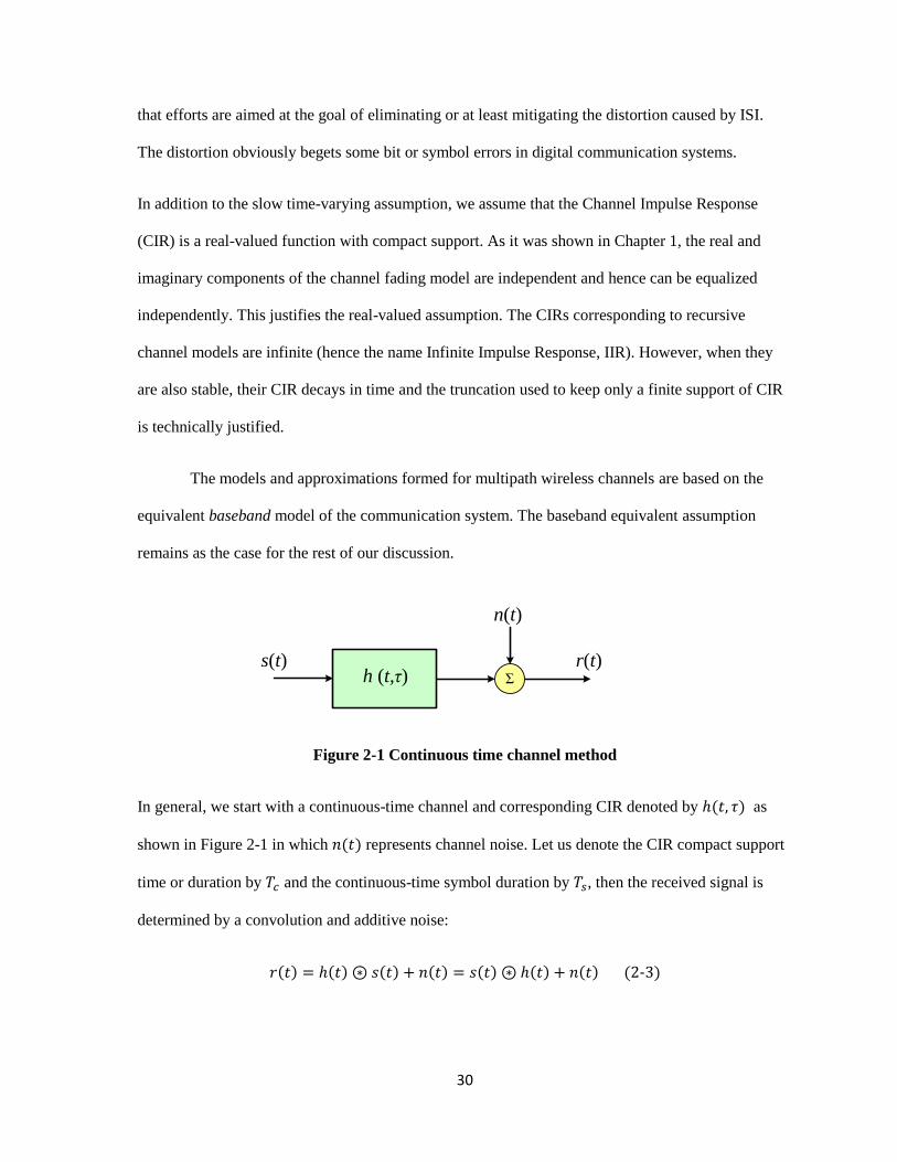
Figure 2-1 Continuous time channel method
In general, we start with a continuous-time channel and corresponding CIR denoted by ( ) as
shown in Figure 2-1 in which ( ) represents channel noise. Let us denote the CIR compact support
time or duration by and the continuous-time symbol duration by , then the received signal is
determined by a convolution and additive noise:
( ) ( ) ( ) ( ) ( ) ( ) ( ) ( )

31
( ) ∫ ( ) ( ) ( )
∫ ( ) ( ) ( )
( )
The convolution is symbolized by in the above equation. The time duration of the received signal
is . We can adjust our derivation for digital communication in which signals are
appropriately sampled and the baseband equivalent system is assumed to generate signal samples at
each sample time , where is the sampling period. In digital communication systems the
samples are taken at each symbol time (occasionally called baud rate or symbol rate systems) that is,
the sampling period and the symbol time are equal. Consequently, the CIR can be written as a
discrete-time impulse response ( ) . It is noteworthy that
there are two main assumptions about CIR, that it can be considered constant relative to equalization
time (slow-varying), and causal (the matter of the choice for the time reference). Furthermore, the
transmitted and received signals are shown in discrete-time by their samples at the time step,
[ ] ( ) [ ] ( ).
r[k]h Σ
n[k]
s[k] x[k]w
Decision
Device
g[k] u[k] = s[k-d]
Channel Model Equalizer
Figure 2-2 Discrete-time model of channel
The channel transfer function is consequently denoted by ( ) that in general can be of Infinite
Impulse Response (IIR) when the model is recursive and of Finite Impulse Response when the model
is non-recursive. In either case, the discrete-time channel is approximated by a transversal filter with
finite length
The ideal equalization, or channel inversion, is to estimate the weight vector of a transversal filter of
finite length denoted by so that it approximately realizes the transfer function ( ) ( ).
32
As was mentioned earlier, a perfect equalization requires a doubly-infinite equalizer. The ideal
transfer function, or at least an approximation of it, is achieved when the weight or state vector of the
equalizer attains some optimum value . This means that ( ) ( ) when ( )
( )| ( ) and ( ) ( )| ( ) are the frequency responses of the channel and the
equalizer respectively. It is obvious that a non-minimum phase channel transfer function cannot be
satisfactorily equalized with sufficient equalizer delay as its inverse is unstable. Even with the help
of stable linear transversal equalizers, a successful inversion by any possible measure might be far
from the desired response. Even the channel transfer functions with zeros near the unit circle
demonstrate deep-nulls (very low values close to zero) in their frequency response and are hard to
equalize. The Zero-Forcing equalizer can be computed for the minimum phase channels if its
transfer function or equivalently CIR is known in the MS (Minimum Squares) sense (see Chi, et.al.
(2006), pp. 188, Ding (2001), pp. 39):
( ) ( )
| ( )|
( )
In Equation (2-5), represents the zero-mean input data variance that is also assumed to be WSS
(Wide Sense Stationary), is the variance of the zero-mean channel noise process that is
independent of the input data. The channel should be stable.
The channel and the linear equalizer system functions ( ) and ( ); for the input signal and the
channel noise can be expressed by:
( ) ( ) ( ) ( ) ( ) ( )
In Equation (2-6) it has been assumed that the channel noise samples are iid and white. The ideal
equalization can be symbolized by ( ) ( ) for some positive integer delay . In the
time domain the equivalent of the channel (CIR) and the equalizer together is a convolution:

33
( )
The result of the convolution in Equation (2-7) has components computed as:
∑
∑
( )
The time-domain equivalent of the ideal equalization is therefore given by the desired response
. It means that the effect of the channel and the equalizer together generates for
and . The only non-zero component is also known as the cursor.
The ideal target of the inversion cannot be achieved with finite-length equalizer filters, so instead of
seeking perfectly zero components, has many non-zero but hopefully very small weights other
than the main delayed weight or the cursor.
The operation of such inversion also has been known as seismic deconvolution (see Clarckson (1993,
pp. 112), Chi, et.al. (2006, pp.188)). In seismic deconvolution, an acoustic waveform called seismic
wavelet is applied at a shot point using special transducers, and then propagated through the terrain
sub-layers. The collected seismic traces are carefully aligned and recorded in seismograms. The
seismograms are then processed in an offline mode to discover the sub-layer’s structure. Seismic
deconvolution is very similar to channel equalization in concept and provides a rich background of
research literature. Kumar and Lau [31] have successfully applied the deconvolution technique to
very important and commonly used Global Positioning Systems (GPS). Their work has been
followed by other researchers in the GPS application that appeared in [29], [30].
The common algorithm in seismic application is Minimum Entropy Deconvolution (MED). The
process is based on a new vector norm called variamax (see Wiggins (1977), Oldenburg (1981)),
which was followed by Cabrelli’s (1984) studies on a different norm he called D-norm. In fact, MED
methods belong to the class of solutions that utilize Higher-Order Statistics (HOS) implicitly.

34
However since MED is performed offline (performed on recorded seismic waveform traces), it is
different in nature from the real-time and adaptive methods.
Finally, similar to Equation (1-21), the common measure of equalization performance is called
residual ISI, denoted here by . Proakis (2001) has also applied what is called Peak Distortion as
the worst-case residual ISI for the purpose of equalization quality measure.
2.3 Deconvolution of A-Priori Known Systems
This is a general problem pertaining to any system that can be modeled by a linear
transversal filter having a tap-weight vector of finite length. The important point in this case is the
fact that the system impulse response is known given by . We seek the best (optimum in the sense
of reduction) equalizer weight vector so that:
( )
The vector here represents standard basis, that is:
( ) ( )
One can expect the main component or cursor value to be one as compared to because the system
impulse response is usually normalized to unit power, that is ‖ ‖ where represents
the response before normalization.
A better formulation of the deconvolution problem can be obtained by the detailed expansion of
Equation (2-9) as follows (assuming that ):

35
[
]
[
]
[ ]
( )
Let us denote the matrix in Equation (2-9) by (This matrix is often known as a filtering matrix).
The filtering matrix has dimensions of ( ) ( ) that renders Equation (2-9) as an
over-determined system of equations. The solution in Least Square (LS) sense is simply given by the
normal equation, symbolically:
( ) ( )
By inspecting Equation (2-11) for the filtering matrix, it is obvious that it has complete rank of
order and hence the matrix of the size is positive-definite and has complete rank,
consequently ( ) exists, and the normal equation in (2-12) has a solution (It is well-known in
linear algebra that positive definite matrixes are invertible with positive-definite inverses).
Although the matrix inversion is computationally costly, for the case of knowing the impulse
response it will be done once, and most likely, in an offline mode.
Efficient algorithms are available for numerical computation of the solution to the normal equations
(see Golub (1996), pp. 237, 545) for numerical methods and analysis).
In most of the practical cases, the system is not a priori-known; in our case for wireless channels that
means the CIR is not known.
36
2.4 Adaptive Algorithm for Equalization of A Priori-Unknown Channels
Although knowledge of the channel is necessary for reliable communication in most modern
systems, this information is not a-priori known and has to be acquired usually by some recursive
adaptation algorithm. One might try to discover, at the least, important channel characteristics by the
application of an adaptive identification algorithm and subsequently apply one of the solutions for
the equalizer filter if necessary.
A more efficient and direct approach is to search for the best possible equalizer weight vector
adaptively, without identifying the channel in advance. The equalization algorithms for unknown
channels are divided into the supervised mode in which a training or pilot sequence known by the
receiver is transmitted. Training period apparently takes part of the available air time and bandwidth,
and it might be very inefficient or even unfeasible in multi-user environments. In spite of wasting
resources, supervised techniques are simple and have guaranteed success in convergence. Qureshi
(1982, 1985) has provided excellent references and tutorials on supervised adaptive equalization.
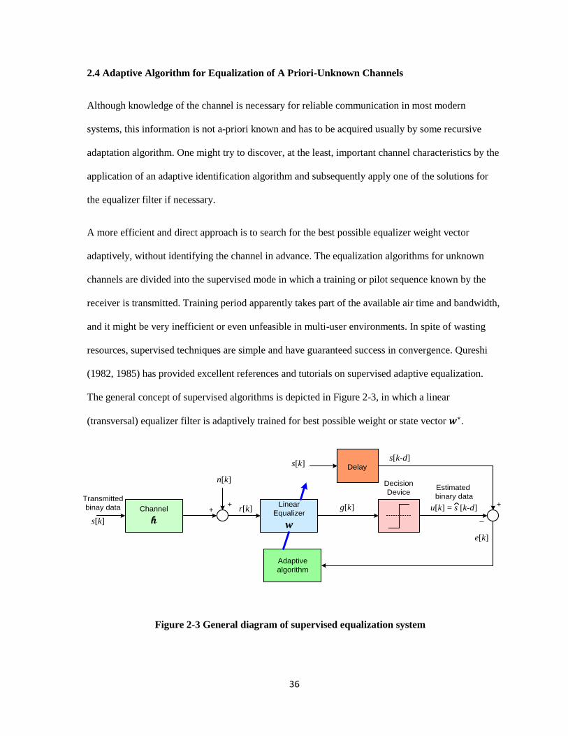
The general concept of supervised algorithms is depicted in Figure 2-3, in which a linear
(transversal) equalizer filter is adaptively trained for best possible weight or state vector .
Channel
h
Linear
Equalizer
w
Adaptive
algorithm
Estimated
binary data
Decision
DeviceTransmitted
binay data ++
_
+
s[k]
n[k]
g[k]
e[k]
u[k] = s [k-d]
s[k-d]Delay s[k]
r[k]
Figure 2-3 General diagram of supervised equalization system
37
Most cellular standards incorporate some kind of training signal. The training sequence in this case is
used to estimate the CIR, then the inverse of the estimated CIR is determined in order to correct the
distortion caused by ISI. Once the equalization is performed to attain a sufficiently low residual
channel ISI, the receiver detected data replaces the training signal in the adaption process to correct
for slow time-variation of the wireless multipath channel.
In blind equalization techniques, the channel equalization or estimation is based solelyon the
received signal samples. It is also assumed that statistical properties of the input data to the channel
are known and incorporated in the corresponding computations.
2.5 Blind Equalization Algorithms
There are several families of algorithms applied to the problem of blind (unsupervised)
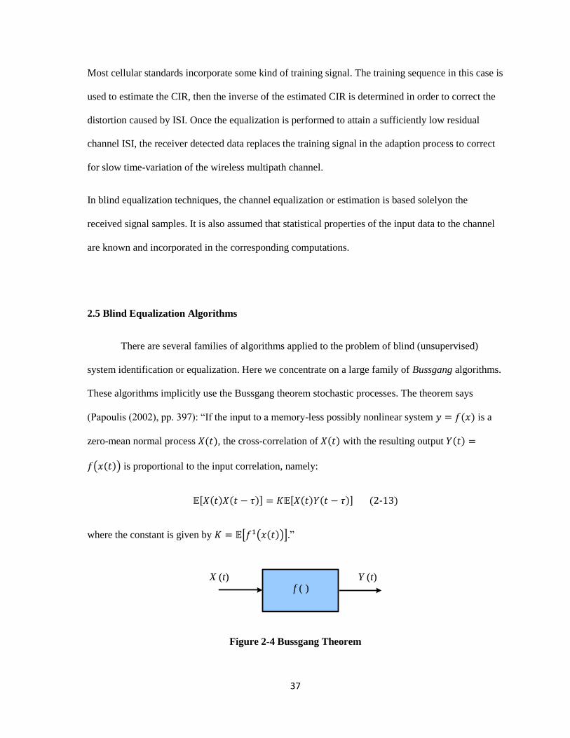
system identification or equalization. Here we concentrate on a large family of Bussgang algorithms.
These algorithms implicitly use the Bussgang theorem stochastic processes. The theorem says
(Papoulis (2002), pp. 397): “If the input to a memory-less possibly nonlinear system ( ) is a
zero-mean normal process ( ), the cross-correlation of ( ) with the resulting output ( )
( ( )) is proportional to the input correlation, namely:
[ ( ) ( )] [ ( ) ( )] ( )
where the constant is given by [ ( ( ))] ”
Y (t)f ( )
X (t)
Figure 2-4 Bussgang Theorem

38
The Bussgang algorithms are named such since all of them use a non-linear (memory-less) function
as a decision device to properly estimate the channel input data. In the case of binary data, the
decision device is simply a slicer that is [ ] ( [ ]) where ( ) represents signum or sign
function (see Figure 2-4). The estimated data is often used instead of any a-priori known training
sequence.
Channel
h
Linear
Equalizer
w
Adaptive
algorithm
Estimated
binary data
Decision
DeviceTransmitted
binay data ++
_
+
s[k]
n[k]
g[k]
e[k]
u[k] = s [k-d]
s[k-d]Delay s[k]
Q( . )
Decision
Feedback
Training
r[k]
Figure 2-5 Basic linear equalization system
In Figure 2-5, a switch is available to change the mode of the algorithm from supervised (training) to
blind mode, or the other way around. We continue to assume that channel variation in time is slow
and, for the purpose of the following discussion, constant. The received signal samples are computed
as follows:
[ ] ∑ [ ] [ ]
( )
[ ] [ ] [ ] ( )
In Equation (2-15), [ ] ( [ ] [ ] [ ]) is the vector of the input symbols, or
data to the channel in the size of the CIR. The equalizer output can be similarly computed by the
received signals:
39
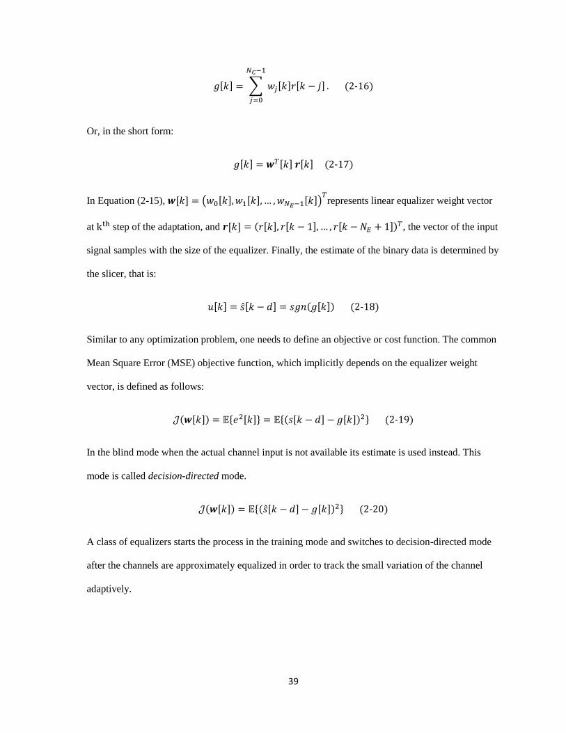
[ ] ∑ [ ] [ ]
( )
Or, in the short form:
[ ] [ ] [ ] ( )
In Equation (2-15), [ ] ( [ ] [ ] [ ])
represents linear equalizer weight vector
at step of the adaptation, and [ ] ( [ ] [ ] [ ]) , the vector of the input
signal samples with the size of the equalizer. Finally, the estimate of the binary data is determined by
the slicer, that is:
[ ] [ ] ( [ ]) ( )
Similar to any optimization problem, one needs to define an objective or cost function. The common
Mean Square Error (MSE) objective function, which implicitly depends on the equalizer weight
vector, is defined as follows:
( [ ]) { [ ]} {( [ ] [ ]) } ( )
In the blind mode when the actual channel input is not available its estimate is used instead. This
mode is called decision-directed mode.
( [ ]) {( [ ] [ ]) } ( )
A class of equalizers starts the process in the training mode and switches to decision-directed mode
after the channels are approximately equalized in order to track the small variation of the channel
adaptively.
40
One important feature of blind methods in the Bussgang class is the relatively simple procedures.
They can use the well-known Least Mean Squares (LMS) method that is probably the simplest
technique among the recursive adaptation for optimization (Widrow, 1985).
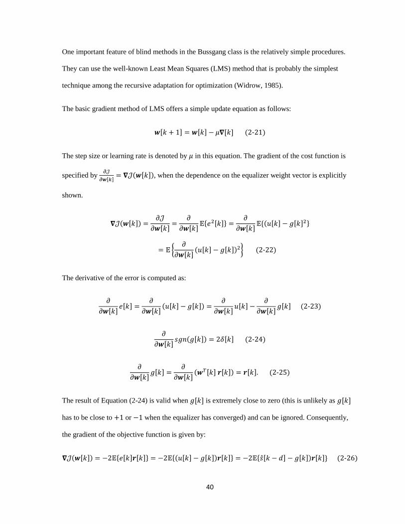
The basic gradient method of LMS offers a simple update equation as follows:
[ ] [ ] [ ] ( )
The step size or learning rate is denoted by in this equation. The gradient of the cost function is
specified by
[ ] ( [ ]), when the dependence on the equalizer weight vector is explicitly
shown.
( [ ])
[ ]
[ ] { [ ]}
[ ] {( [ ] [ ] }
{
[ ]( [ ] [ ]) } ( )
The derivative of the error is computed as:
[ ] [ ]
[ ]( [ ] [ ])
[ ] [ ]
[ ] [ ] ( )
[ ] ( [ ]) [ ] ( )
[ ] [ ]
[ ]( [ ] [ ]) [ ] ( )
The result of Equation (2-24) is valid when [ ] is extremely close to zero (this is unlikely as [ ]
has to be close to or when the equalizer has converged) and can be ignored. Consequently,
the gradient of the objective function is given by:
( [ ]) { [ ] [ ]} {( [ ] [ ]) [ ]} { [ ] [ ]) [ ]} ( )

41
The simplicity of the LMS technique lies in the fact that it takes the simplest possible estimate (and
probably not quite accurate gradient by just removing the expectation operator. That is
{
[ ] [ ]}
[ ] [ ] [ ] [ ] ( )
Consequently, updating the equalizer weight vector simplifies to the following one (the coefficient 2
in (2-27) is absorbed in the step size :)
[ ] [ ] ( [ ]) [ ] [ ] [ ] ( )
2.6 Bussgang Algorithms
We consider the overall channel and the equalizer system for which a transversal filter with
finite number of taps is used as the linear equalizer in Figure 2-6.
Channel
h
Linear
Equalizer
w
Estimated
binary data
Decision
DeviceTransmitted
binay data ++
s[k]
n[k]
g[k]Q( . )
r[k]
u[k] = s [k-d] = Q(g[k]) x[k]
Figure 2-6 Basic equalization system
As was mentioned earlier, the channel noise sample [ ] is relatively small compared to ISI measure
and its effects are not considerable until most of ISI has been removed. Consequently, one may
ignore the channel noise: that means [ ] [ ], where [ ] is the noise-free signal at the
receiver. Once again, we assume that the CIR (Channel Impulse Response) represents the transmitter
filter, multipath channel, and the receiver filter together.

42
[ ] [ ] ∑ [ ] [ ]
[ ] ( )
[ ] [ ] [ ] ∑ [ ] [ ]
[ ] ( )
In the above equations the subscript k indicates the vector values at the k-th step. The subscript k in
the equalizer weight vector could be dropped for convenience and be considered as implied when
it simplifies the equations. Equation (2-30) can be expanded as
[ ] [ ] [ ] ∑ [ ] ∑ [ ] [ ]
( )
Let denote the best (optimal) weight vector of the linear equalizer. Equation (2-30) can be written
including the optimum weight vector.
[ ] ∑ [ ] [ ]
∑ [ ]
∑ ( [ ] ) [ ]
( )
The first term on the right-hand side in (2-32) is the optimum equalized signal representing the
correct estimate of [ ], the appropriately delayed input signal to the channel.
∑ [ ]
[ ] ( )
The constant coefficient in (2-33) is the cursor value (see Equation (2-7)). The second term in (2-
32) is the undesired remainder and is known as convolution error.
[ ] ∑ ( [ ] ) [ ]
∑ [ ] [ ]
( )

43
The convolution error is approximated to be zero-mean, Gaussian, and independent of the input
sequence [ ] (See Nandi 1999).
The final block in Figure 2-5 in most of the implementations is a memoryless (zero-memory)
nonlinear device, whose function is denoted by ( ). As will be discussed the choice of nonlinear
function has a major impact on the performance of the algorithm to which it belongs. In the case of
the system with binary input data we used a slicer ( ( ) Function) for the zero-memory
nonlinearity.
Having explained the general setup for linear equalizers, we turn our attention to the Bussgang
family of algorithms. Haykin (2002) and Ding, et.al. (2001) have provided great expositions of the
general Bussgang algorithms as the foundation for most of the known techniques in linear
equalization. Let us reconsider the effect of the channel and the equalizer together by their
convolution denoted by [ ] [ ]:
[ ] ∑ [ ]
( )
[ ] ∑ [ ] [ ]
[ ] [ ] [ ] ( )
In (2-7) and (2-33) we have denoted the cursor value after the algorithm has converged by [ ]
and then the convolution error is as follows:
[ ] ∑ [ ] [ ] ( )
Equation (2-37) is just a reformulation of (2-34) in terms of the convolution samples [ ].

44
When the equalizer has converged to the final point, Equation (2-36) should become [ ]
[ ] [ ] with the minimum possible value for the convolution error. When the distribution
(pdf) of [ ] is known the decision device is a Maximum A-Posteriori (MAP) estimator as defined in
the following equation.
[ ]
[ ]| [ ]( [ ]| ) ( )
When the distribution of [ ] is not available, in particular the conditional probability in (2-38) is not
known, the same approximations are made based on the assumptions that the input sequence [ ] is
zero-mean iid. Consequently the [ ] [ ] terms in [ ] (Equation 2-38) are independent and
have finite variance so that the application of the central limit theorem implies that the [ ]
distribution is approximately Gaussian and is independent of [ ]. The [ ] process is also
assumed to be zero-mean and its variance can be computed with the knowledge of the variance of the
input data sequence (namely ) as follows.
∑| [ ]|
( )
By considering [ ] as the equalizer output noise with the variance given by (2-39), the optimum
memoryless nonlinearity in the sense of MAP will be the minimum variance estimation as in
Equation (2-40) (see Ding (2001), pp. 48):
( [ ]) [ ] { [ ]| [ ]} ( )
The signal-to-noise ratio at the output of the equalizer can now be computed easily by:
{| [ ]| }
( )

45
{| [ ]| } in (2-41) represents the input sequence power. The information in Equation (2-41) must
be known in order to find the nonlinearity function ( ) and when such information is not available
or difficult to estimate, the Bussgang algorithms are no longer optimum (for detailed ZNL
determination see Ding (2001), pp. 49). Finally when the nonlinearity has been determined, one can
iteratively solve for the equalizer weights in the Least Squares (LS) sense using the following update
equation:
[ ] ( { [ ] [ ]}) { [ ] ( [ ] [ ])} ( )
The simple and popular adaptive method is the gradient descent algorithm that can be employed for
finding the optimal weight vector with the following update equation.
[ ] [ ] ( ( [ ]) [ ]) [ ] ( )
In the recursive methods of Equations (2-42) and (2-43) is assumed to be the noise-free signal at
the receiver.
It has been shown that when the equalizer is converged, the output satisfies the Bussgang condition
{ [ ] [ ]} { [ ] ( [ ])} ( )
A final point to be made is that the convergence of the Bussgang algorithm is mostly unknown.
Godfrey (1981) has proved the local convergence of the Bussgang algorithms.
Almost all of the linear equalization techniques that we review in this section are based on the same
basic concept except for the choice of zero-memory nonlinearity device. They are similar in the use
of gradient descent and LMS (Least Mean Square) algorithm for their iterative adaptation process.

46
The Sato Algorithm
The Sato algorithm is perhaps the simplest technique used for the problem of blind equalization and
was introduced early in the rich research history. It is also among the algorithms categorized as
Decision-Directed Equalizers (see Figure 2-7.)
Channel
h
Linear
Equalizer
w[k]
Adaptive
algorithm
Estimated
binary data
Decision
DeviceTransmitted
binay data ++
_
+
s[k]
n[k]
g[k]
e[k]
u[k] = s [k-d] x[k] r[k]
Figure 2-7 Basic Decision Feedback Equalizer diagram
This algorithm and some improved versions of it that are mentioned here are appropriate for PAM
(Pulse Amplitude Modulation), including the simple binary case (2-PAM) for which the nonlinearity
is simply ( ) ( ). The cost function that was chosen by Sato without any theoretical
justification was:
( [ ]) {( [ ] ( [ ])) } ( )
The important parameter in (2-45) is the choice of that is given in Equation (2-47). The update
equation, based on gradient descent method will therefore be given by the following equation:
[ ] [ ] ( [ ] ( [ ])) [ ] ( )
In the update equation the coefficient of ½ of the gradient is absorbed in the step size . The Sato
choice for was intuitively selected as:
47
{| [ ]| }
{| [ ]|} ( )
The only information necessary for this choice is the input data statistics that are assumed to be
known in advance. The Sato algorithm can be compared to the simple LMS algorithm:
[ ] [ ] ( [ ] [ ]) [ ] ( )
where the delayed input estimate is determined as [ ] ( [ ]). Consequently, the only
difference is that in the LMS algorithm. In fact, the success (convergence) of the Sato
algorithm has been attributed to the choice of . Hence, it is clear that the convergence of the Sato
algorithm depends on the probability of the event when the sign of the real error [ ] [ ]
and its estimate [ ] ( [ ]) agree. Sato’s method was intended for one-dimensional multi-
level PAM, in particular for the case of binary 2-level signaling. The Benveniste-Goursat-Ruget
theorem for convergence (Haykin (2002), pp 716, 717) with the assumption of doubly-infinite filter
size applies to Sato’s method. The theorem states that the global convergence of the Sato can be
gained for the input distributions of continuous non-Gaussian or sub-Gaussian in particular
uniformly distributed input sequences. Macchi (1985) and Mazo (1980) have shown that the Sato
algorithm converges to local minima for QAM (Quadratic Amplitude Modulation) input signals
instead of the optimum global minimum. Moreover, Ding, et.al. (1989) have shown the possible
convergence to any local minima for multi-level signaling as well.
The Godard Algorithm
Godard (1980) proposed a family of Constant-Modulus Algorithms (CMA) for blind equalization in
general M-ary QAM systems. The QAM systems are collectively known as two-dimensional digital
communications. The main idea is to use a cost function that depends only on the magnitude of the
48
equalizer output, that is to say that the cost function is independent of the equalizer output phase. The
p-th order cost function (where p is a positive integer) is defined by:
( [ ])
{(| [ ]| )
} ( )
The new Godard parameter is a positive and real constant.
{| [ ]| }
{| [ ]| } ( )
It seems that the unavailable input sequence [ ] in the error samples is replaced by the constant ,
which contains the information about the input data distribution. In other words, the Godard
algorithm is designed to measure the deviation of the equalizer output [ ] from a constant modulus
and use it for adaption.
The error signal for the general p-th order is given by
[ ] (| [ ]| )| [ ]| [ ] ( )
The corresponding update equation will be written as
[ ] [ ] [ ] [ ] ( )
In the case of , the cost function reduces to one that can be considered as a modified Sato
algorithm.
( [ ]) {(| [ ]| )} {| [ ]| }
{| [ ]|} ( )

49
The cost function for the case of is CMA (Constant-Modulus Algorithm), which is well-
known in the literature. Equation (2-54) is the corresponding cost function and the modulus
parameter for this important case:
( [ ]) {(| [ ]| )} {| [ ]| }
{| [ ]| } ( )
The CMA algorithm is intended for systems in which the symbols have the same amplitude
(constant) with different phases in the corresponding constellation of the QAM system and cannot be
used for multi-level PAM cases. In conclusion, we remark that the Godard algorithm performs better
than the other Bussgang algorithms in the MSE sense. The algorithm can equalize a dispersive
channel even when the eye (of eye-pattern) is not initially open (Haykin (2002), pp 724).
Many researchers have challenged the problem of blind equalization or of the system identification,
and their effects have culminated in many algorithms, each with some advantages. Of these
algorithms, many belong to the family of Bussgang algorithms in which the zero-memory
nonlinearity has the Bussgang property.
BGR (Benveniste-Goursat-Ruget) is an extension to the Sato algorithm with the goal of pushing the
start-up adaptation from the local (that is near) of the optimal tap weights (it was mentioned that the
Sato algorithm has sure convergence when the initial weights are close to the global optimum point.)
Stop-and-Go algorithm by Picchi and Prati (1987) basically implements the same adaptation as
Sato’s and the following technique except that the adaptation at each iteration can be skipped (no
change to the state vector) based on the examination of some condition that flags possible incorrect
estimates. This, for instance, can be done by comparing the sign of two different errors each
belonging to a different algorithm of this family.

50
2.7 References
[1 ] Benveniste, A., Goursat, M., Ruget, G., “Robust Identification of Nonminimum Phase
Systems: Blind Adjustment of Linear Equalizer in data Communications”, IEEE Transactions
on Automatic Control, Vol. AC-25, No. 3, 1980.
[ 2] Bussgang, J.J., “Cross-correlation function of amplitude distorted Gaussian signals”, Tech.
Rep. 216, MIT, 1992.
[3 ] Cabrelli, C.A., “Minimum Entropy Deconvolution and Simplicity: A Noniterative Algorithm”,
geophysics, Vol. 50, No. 3, March 1984.
[4 ] Chi, et.al., “Blind Equalization and System Identification”, Springer-Verlag, London, 2006.
[ 5] Ding, Z., Li, Y., “Blind Equalization and Identification”, Marcel Dekker, 2001.
[6] Diniz, P.S.R., “Adaptive Filtering Algorithms and Practical Implementation”, Springer, New
York, 2010.
[7] Friedman, M., Savage, L.J., “Experimental determination of the maximum of a function”,
Selected Techniques of Statistical Analysis, McGraw-Hill, New York, 1947.
[8] Freidman, S. “On stochastic approximation”, Ann. Math. Stat. 34, 1963.
[9 ] Godfrey, R., Rocca, F., “Zero-memory nonlinear deconvolution”, geophysical Prospecting,
No. 29, 1981.
[10 ] Godard, D.N., “Self-Recovering Equalization and Carrier Tracking in Two-Dimensional Data
Communication Systems”, IEEE Transactions on Communications, Vol. COM-28, No. 11,
November 1980.
[11] Haykin, S., “Adaptive Filtering Theory”, 4th Edition, Prentice-Hall, New Jersey, 2002.

51
[12] Hotelling, H., “Experimental determination of the maximum of a function”, Ann. Math. Stat.
12, 1941.
[13] Kiefer, J., Wolfowitz, J., “Stochastic estimation of the maximum of a regression function”,
Ann. Math. Stat. 23, 1952.
[14] Kumar, R., Moore, J.B., “Adaptive Equalization via Fast Quantized State Method”, IEEE
Transactions on Communications, Vol. COM-29, No. 10, October 1981.
[15] Kumar, R., Moore, J.B., “State Inverse and Decorrelated State Stochastic Approximating”,
Automatica, Vol. 16, may 1980.
[16] Kushner, H.J., “Adaptive technique for the optimization of binary detection systems”, 22G-2
Lincoln Laboratories, MIT 1962.
[17] Kushner H.J., Yin, G.G., “Stochastic Approximation and Recursive Algorithms and
Application”’ 2nd
Edition, Springer-Verlag, New York, 2010.
[18] Macchi, O., Eweda, E., “Convergence Analysis of Self-Adaptive Equalizers”, IEEE
Transaction on Information Theory”, Vol. IT-30, No. 2, March 1984.
[19] Mazo, J.E., “Analysis of decision-directed convergence”, Bell Systems Tech., Vol. 59, pp.
1857-1876.
[20] Nandi, A.K., “Blind Estimation using Higer-Order Statistics”, Kluwer, 1999.
[21 ] Oldenburg, D.W., Levy, S., Whittall, K.P., “wavelet Estimation and Deconvolution”,
Geophysics, Vol. 46, No. 11, Nov. 1981.
[22] Papoulis, A., Unnikrishna Pillai, S., “Probability, random Variables, and Stochastic
Processes”, McGraw-Hill Higher Education, 2002.

52
[23] Picchi, G., Prati, G., “Blind Equalization and carrier Recovery using a “Stop-And-Go”
Decision-Directed Algorithm”, IEEE Trans. on Comm., Vol. COM-25, No. 99, Sept. 1987.
[24] Proakis, J.G., “Digital Communications”, 4th Edition, McGraw-Hill Higher Education, 2001.
[25] Robbins, H., Monro, S., “A Stochastic approximation method”’ Ann. Math. Stat. 22 (1951).
[26] Wasan, M.T., “Stochastic Approximation”’ Cambridge University Press, Cambridge, 1969.
[27] Widrow, B., Stearns, S.D., “Adaptive Signal Processing”, Prentice-Hall, New Jersey, 1985.
[28] Wiggins, R.A., “Minimum Entropy Deconvolution”, Geoexploration, Vol. 16, 1978.
Additional References:
[29] Dragunas, K., Borre K, “Multipath Mitigation Based on Deconvolution,” Journal of Global
Positioning Systems, Vol. 10, No. 1, 2011.
[30] Dragunas, K., Borre K, “Indoor Multipath Mitigation,” Ubiquitous Positioning Indoor
Navigation and Location Based Services (UPINLBS), 2010, pp. 1-8.
[31] Kumar, R., Lau, K., “Deconvolution Approach to Carrier and Code Multipath Error
Elimination in High Precision GPS,” Proceedings of the 1996 National Technical Meeting of
the Institute of Navigation, Santa Monica, CA., pp. 729-737,.

53
Chapter 3: Blind Channel Equalization using Diversified Algorithms
3.1 Introduction
Blind techniques in wireless channel equalization are diversified and abundant; nonetheless,
a robust and fast convergent technique with reasonably efficient computations remains as an open
problem. We have briefly reviewed most of these techniques but not all of them in Chapter 2. In
particular Fractionally-Spaced Equalization (FSE) and the algorithms using Higher Order Statistics
(HOS) were not visited. The reason of such negligence is the fact that various techniques of FSE and
HOS are computationally costly and our target systems with multiple algorithms need to employ
relatively simple methods to keep overall computational cost of the system affordable. Our new
conception in the blind or unsupervised equalization is to employ two or more of the simple
algorithms in a cooperative scheme3 to increase the probability of convergence of the overall system
comprising multiple of algorithms. Figure 3-1 shows the proposed arrangement that includes three
separate equalizers generating and sharing one final estimate of binary data.
Channel
h
Blind
Equalizer 2
w2[k]
Decision and
Adaptive
algorithms[k]
Channel noise
Transmitted binay or PAM
symbols ++
Slicer
Blind
Equalizer 1
w1[k] Slicer
Blind
Equalizer m
w3[k] Slicer
n[k]
g1[k]
r[k]
g2[k]
g3[k]
s1[k-d]
s2[k-d]
s3[k-d]
s [k-d]
Final symbol estimate
Figure 3-1 Blind equalizer system with diversified algorithms
3 The multiple algorithm architecture for adaptive signal processing was invented by Dr Rajendra Kumar, and is in the
process of being patented. Here the performance analysis of one of the various possible forms of this architecture for the
blind mode equalizer is presented.

54
3.2 Recursive Least Squares Adaptive Algorithms
In this section we give a brief introduction to a family of algorithms known as Recursive
Least Squares (RLS). RLS algorithms incorporate the inverse of the covariance matrix of the process
(wireless channel in our case) in the update equation that resembles the Wiener optimum filter
solution, or Newton-like algorithms in adaptive techniques. Its final performance measures are often
poor as we will explore in sections 3.4 and 3.5 of this chapter. RLS techniques and the resulting
ramifications are well-known and long lasting. The references [1, 3, and 6] give comprehensive
origin and proofs of the methods. A closely-related application of RLS in the area of digital
communications is given in [2].
Consider the problem of iteratively adjusting the weight vector of a transversal filter used to equalize
a wireless channel. Figure 3-2 depicts a general system setup in which the received signals are
generated by a process that could be the unknown wireless communication channel.
Linear
Equalizer
w [k]
Recursive
Least Squares
Algorithm
_ +
r [k]
d [k]
e [k]
wT[k]r[k]
Figure 3-2 General Recursive Least Squares algorithm
The inputs to the transversal filter are collected in a vector of the size of the filter denoted by
[ ] ( [ ] [ ] [ ]) . We have used exactly the same vector as the baseband
samples of the received signals input to the channel equalizer in Chapter 2.

55
An approximate estimate of the auto-covariance matrix of the process generating the input vector
[ ] at step k is computed by
∑ [ ] [ ]
( )
The computation of the running estimate of is simplified, commonly as follows.
(
) (
) [ ] [ ] ( )
The basic weight vector update equation for the RLS type of algorithm includes the inverse of the
covariance matrix. This equation for advancing to the next step from step can be written as:
[ ] [ ] ( )
In Equation (3-3), is the step size and in common RLS implementations is usually equal to one,
and the error is computed as the difference of the desired output [ ] and the filter output.
[ ] [ ] [ ] [ ] ( )
The inverse covariance matrix required for the weight vector update equation needs to be updated in
each step using the running update Equation (3-2).
( [ ]
[ ]) ( )
To avoid costly matrix inversion at each step of adaptation the famous Woodbury’s matrix inversion
identity is used to obtain
[ ] [ ]
[ ] [ ]
( )

56
For simplicity the inverse matrix is denoted by and the last equation simplifies to the
following.
[ ]
[ ] [ ] [ ]
( )
The update equation becomes
[ ] [ ] ( )
It has been recommended (See Clarkson [1]) to initialize the weight vector to a zero vector
and the inverse covariance matrix to a large diagonal matrix where is a small constant .
Exponentially Weighted Recursive Least Squares
A popular variation of the RLS algorithm is the Exponentially Weighted version (EWRLS) in which
a forgetting factor usually close to one is used to reduce the effects of relatively old received
information. Specifically in the channels that are modeled by limited-size transversal filters the
correlation between the recently received signals and the ones belonging to many steps backward is
trivial if not zero, hence the application of forgetting factors in Exponentially Weighted RLS of the
range of to has been shown to have favorable results, in particular n case of
time-varying channels. The EWRLS algorithm equations incorporating the forgetting factor are
similar to those for regular RLS and are summarized in the following ( ).
[ ] [ ] ( )
[ ] [ ] ( )
(
[ ] [ ]
[ ] [ ]) ( )

57
[ ] [ ] ( )
Quantized-State Recursive Least Squares
Kumar and Moore in their 1981 paper [4] proposed four different algorithms that are similar in
structure as the RLS algorithms to simplify the computational effort and speed up the convergence.
These Quantized-State (QS) algorithms have been successfully applied to some problems ever since
(for example see Kumar and Khor [5]).
The first two of the QS algorithms are based on a sliced version of the input signal vector [ ], in
which each element is determined by [ ] ( [ ]). Consequently all elements of the input
vector (also known as state) belong to the binary field of { }, and together as a vector they are
called the quantized state. The differences between the two proposed Quantized-State algorithms are
easily seen in the following summary of the sets of recursive equations.
Quantized-State 1 (QS-1):
[ ] [ ] ( )
(
[ ] [ ]
[ ] [ ]) ( )
[ ] [ ] ( )
Quantized-State 2 (QS-2):
[ ] [ ] ( )
(
[ ] [ ]
[ ] [ ]) ( )
[ ] [ ] ( )

58
In all of the above equations the error at step is [ ] [ ] [ ] [ ]. It should be clarified
that the learning rate in QS algorithms has different effect and purpose compared to the LMS, and
RLS algorithms. The learning rate or as often called step size in the LMS algorithm determines the
stability (see Widrow [7] or [8]).
It is well-known that for stationary processes the covariance matrix is symmetric and Toeplitz. The
inverse of the covariance matrix however is symmetric but not completely Toeplitz. Kumar and
Moore have used this fact to further speed up the required computation. This method leads to another
two algorithms in their paper [4] that are not being applied in this chapter.
The concentration of this chapter is not to evaluate the performance of the individual algorithms,
which have their own distinguished advantages exemplified and documented in the corresponding
literature.
A good example is QS algorithms, form which the QS-2 is used in cooperation with other
algorithms. In practice for QS algorithms the step size should be adjusted and the number of taps
in the equalizer be increased to achieve quality performance, however QS-2 has been used for
cooperation and no particular adjustment to corresponding parameters is made.
3.3 General Cooperative Adaptive System with Diversified Algorithms
The concept of devising multiple-algorithm system to solve the problem of wireless channel
equalization or other related problems that can be tackled by adaptive algorithms seeks carefully
crafted plans for using the outcome of the contributing algorithms. Since we need to use two or more
techniques, the participating algorithms should not be computationally intensive. Good candidates
having the desired simplicity are LMS, RLS and Quantized-State techniques. The principle idea for
cooperating algorithms is to use majority vote system; however this can only be done for the system
59
having 3 or more methods involved. Moreover, we have to keep the number of algorithms small to
avoid excessive computation at each step of adaptation. Since the system of having only two
algorithms is attractive in terms of required computations, we need to design a different plan for such
systems (see section 3.4).
First we consider the case of 3 algorithms for a binary data system (field of { }): if 2 out of 3
or more of the adaptive processes agree on the estimate of the data in step , the majority wins and
the wining estimate is used for computing the error at that step. Let us denote the probability of
correct data estimate of each algorithm by . The total probability of correct data
estimate of the system based on the majority vote and denoted by is determined as follows.
( ) ( ) ( ) ( )
To see how this technique improves the overall performance of the system we need to have a
reasonable estimate for . We argue that if one does not make any effort one can
estimate the correct binary data with 0.5 probability, say using a uniform random number generator.
We fairly assume that when one makes some effort by signal processing to perform better, the
probability of a correct estimate goes up by a very small amount, say 0.5%. Now for simplicity we
assume that the probability of the algorithms are equal and .
( )
We further assume that in theory the correct estimate of the data at step leads to the correct error
calculation used for updating the weight vector that in turn results in a slightly better estimation
probability in next step . Using this assumption we can run the system for a few steps and
compute the probability of the correct performance as shown in Figure 3-3. As it can be seen in
Figure 3-3 at least in theory we can achieve a fast improving system. In fact this needs to be
evaluated by simulations (see section 3.5).
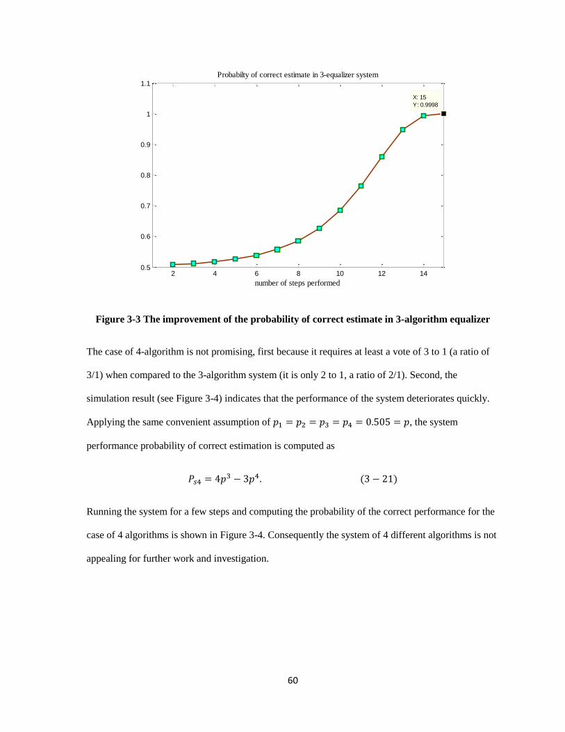
60
Figure 3-3 The improvement of the probability of correct estimate in 3-algorithm equalizer
The case of 4-algorithm is not promising, first because it requires at least a vote of 3 to 1 (a ratio of
3/1) when compared to the 3-algorithm system (it is only 2 to 1, a ratio of 2/1). Second, the
simulation result (see Figure 3-4) indicates that the performance of the system deteriorates quickly.
Applying the same convenient assumption of , the system
performance probability of correct estimation is computed as
( )
Running the system for a few steps and computing the probability of the correct performance for the
case of 4 algorithms is shown in Figure 3-4. Consequently the system of 4 different algorithms is not
appealing for further work and investigation.
2 4 6 8 10 12 140.5
0.6
0.7
0.8
0.9
1
1.1
Probabilty of correct estimate in 3-equalizer system
number of steps performed
X: 15
Y: 0.9998

61
Figure 3-4 The degradation of the probability of correct estimate in 4-algorithm equalizer
Contrary to the 4-algorithm case, the system composed of 5 different algorithms has the benefit of
even lower minimum ratio of 3 to 2 (3/2) vote for majority. Using similar assumptions as in the other
cases, , the system correct estimate probability becomes
( )
The improvement of the estimation, illustrated in Figure 3-5, grows faster with the number of steps
compared to the 3-algorithm case. The drawback of the system with 5 algorithms is the increase in
the amount of computation required, which may significantly reduce its practical application.
1 2 3 4 5 6 70
0.05
0.1
0.15
0.2
0.25
0.3
X: 5
Y: 1.959e-007
Probabilty of correct estimate in 4-equalizer system
number of steps performed

62
Figure 3-5 The improvement of the probability of correct estimate in 5-algorithm equalizer
1 2 3 4 5 6 7 8 9 10 110.5
0.6
0.7
0.8
0.9
1
1.1
Probabilty of correct estimate in 5-equalizer system
number of steps performed
X: 10
Y: 0.9998

63
3.4 Adaptive Systems with Two Algorithms
As was mentioned in section 3.3 the majority vote approach cannot be applied to a system of two
algorithms (Notice that the similar approach as for 3 and more algorithms of
leads to that is disappointing). Hence we need to create a different configuration.
The proposed configuration w chooses the equalizer output with larger absolute value ( ) to
be applied to the slicer that generates the final system estimate of the binary data by
( (| | | |)). The corresponding system configuration is shown in Figure 3-6.
Equalizer 1
w1
Equalizer 2
w2
Channel
hk
Channel noise
Transmitted binary data
++
Select absolutely
larger output
Σ
Σ
Adaptive
algorithm
Adaptive
algorithm
s[k]
g1[k]
g2[k]
n[k]
r[k]
s [k-d]
Final symbol estimate
+
+
-
-
e1[k]
e2[k]
Figure 3-6 The configuration for cooperative 2-algorithm equalizer system
The algorithms selected to be used here are: a very simple LMS algorithm specified in chapter 2 by
Equation (2-21) and (2-28), repeated here for convenience and the computationally more intensive
but faster EWRLS algorithm specified by Equation (3-11) and (3-12) in section 3.2.
[ ] [ ] [ ] ( )
[ ] [ ] ( [ ]) [ ] [ ] [ ] ( )

64
We have examined the proposed configuration on different channels with the equalizers of equal
channel-size (number of taps) in each algorithm. The equalizer can be larger in size, and the size
equal to the length of the channel impulse response. The equalizers of larger size are frequently
designed and used to get better performance (lower residual ISI for example).
Channel 1
The first channel is symmetric with five taps (non-minimum phase) specified by the following
impulse response and the corresponding transfer function
[ ] [ ] [ ] [ ] [ ]
( )
The four channel zeros are located at: , the complex zeros being on the unit
circle.
When the LMS (with ) and EWRLS (with ) are adapting independently, the
corresponding residual ISI for two algorithms is given in Figure 3-7.
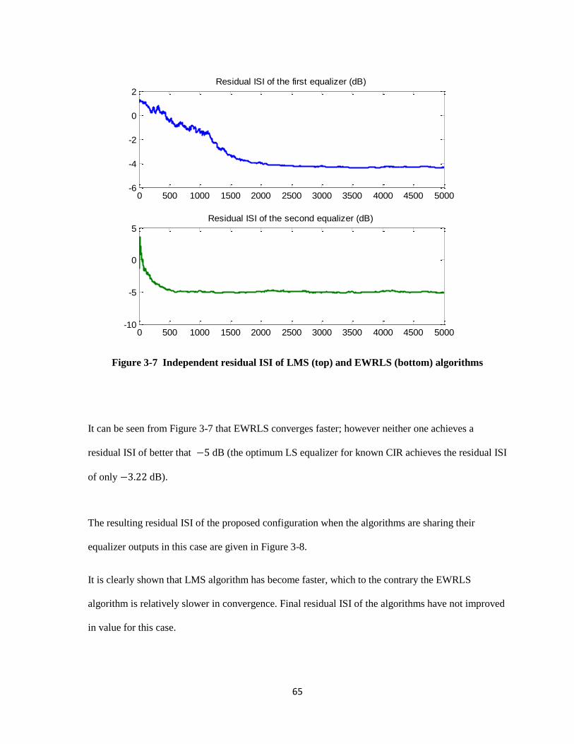
65
Figure 3-7 Independent residual ISI of LMS (top) and EWRLS (bottom) algorithms
It can be seen from Figure 3-7 that EWRLS converges faster; however neither one achieves a
residual ISI of better that dB (the optimum LS equalizer for known CIR achieves the residual ISI
of only dB).
The resulting residual ISI of the proposed configuration when the algorithms are sharing their
equalizer outputs in this case are given in Figure 3-8.
It is clearly shown that LMS algorithm has become faster, which to the contrary the EWRLS
algorithm is relatively slower in convergence. Final residual ISI of the algorithms have not improved
in value for this case.
0 500 1000 1500 2000 2500 3000 3500 4000 4500 5000-6
-4
-2
0
2Residual ISI of the first equalizer (dB)
0 500 1000 1500 2000 2500 3000 3500 4000 4500 5000-10
-5
0
5Residual ISI of the second equalizer (dB)

66
Figure 3-8 Cooperative residual ISI of LMS (top) and EWRLS (bottom) algorithms
The comparison of the results of the LMS and EWRLS algorithms of independent and cooperative
processing of channel 1 are given in Figure 3-9 and 3-10 respectively.
0 500 1000 1500 2000 2500 3000 3500 4000 4500 5000-6
-4
-2
0
2Residual ISI of the first equalizer (dB)
0 500 1000 1500 2000 2500 3000 3500 4000 4500 5000-10
-5
0
5Residual ISI of the second equalizer (dB)

67
Figure 3-9 Comparison of LMS algorithm residual ISI for independent (magenta) and
cooperative (blue) modes
Figure 3-10 Comparison of EWRLS algorithm residual ISI for independent (magenta) and
cooperative (blue) modes
0 500 1000 1500 2000 2500 3000 3500 4000 4500 5000-5
-4
-3
-2
-1
0
1
2
Residual ISI of the first equalizer (dB)
X: 1100
Y: -3.221
X: 1100
Y: -1.598
LMS only
LMS +DA2
0 500 1000 1500 2000 2500 3000 3500 4000 4500 5000-6
-4
-2
0
2
4
6
Residual ISI of the second equalizer (dB)
X: 550
Y: -4.807
X: 550
Y: -1.742
RLS only
RLS + DA2

68
Channel 2
The second channel with eleven taps is specified by the impulse response of
[ ] [ ] [ ] [ ] [ ] [ ]
[ ] [ ] [ ] [ ]
The corresponding transfer function is:
( )
The ten channel zeros are located at :
. This channel is also non-minimum phase.
We let the LMS and EWRLS (with ) algorithms adapt separately and the corresponding
residual ISI of each algorithm in this case is shown in Figure 3-11.

69
Figure 3-11 Independent residual ISI of LMS (top) and EWRLS (bottom) algorithms
It can be seen from Figure 3-11 that EWRLS converges relatively faster, however LMS achieves a
better residual ISI of about dB (the optimum LS equalizer residual ISI of dB).
The residual ISI of the proposed configuration with the cooperating algorithms in this case are given
in Figure 3-12. It can be seen that LMS algorithm has become slightly faster with the same final
residual ISI and so does the EWRLS algorithm that also converges faster with about the same final
residual ISI.
0 500 1000 1500 2000 2500 3000 3500 4000 4500 5000-15
-10
-5
0Residual ISI of the first equalizer (dB)
0 500 1000 1500 2000 2500 3000 3500 4000 4500 5000-15
-10
-5
0
5Residual ISI of the second equalizer (dB)

70
Figure 3-12 Cooperative residual ISI of LMS (top) and EWRLS (bottom) algorithms
The comparison of the results of LMS and EWRLS algorithms in the independent and the
cooperative processing for channel 2 are given in Figure 3-13 and 3-14 respectively.
0 500 1000 1500 2000 2500 3000 3500 4000 4500 5000-20
-15
-10
-5
0Residual ISI of the first equalizer (dB)
0 500 1000 1500 2000 2500 3000 3500 4000 4500 5000-15
-10
-5
0
5Residual ISI of the second equalizer (dB)

71
Figure 3-13 Comparison of LMS algorithm residual ISI for independent (magenta) and
cooperative (blue) modes
Figure 3-14 Comparison of EWRLS algorithm residual ISI for independent (magenta) and
cooperative (blue) modes
0 500 1000 1500 2000 2500 3000 3500 4000 4500 5000-16
-14
-12
-10
-8
-6
-4
-2
0
Residual ISI of the first equalizer (dB)
X: 1000
Y: -5.805
X: 1000
Y: -4.079
LMS only
LMS + DA2
0 500 1000 1500 2000 2500 3000 3500 4000 4500 5000-12
-10
-8
-6
-4
-2
0
2
4
6
X: 400
Y: -5.232
Residual ISI of the second equalizer (dB)
X: 400
Y: 1.009
RLS only
RLS + DA2

72
3.5 Adaptive Systems with Three Algorithms
With a system including 3 different cooperating algorithms the majority vote determines the
final system estimate of the transmitted data and therefore the error for each algorithm is computed
based on this estimate. The equalizer outputs are first applied to a hard-limiter before the votes are
sensed and a minimum ratio of 2 to 1 suffices to win. We have shown with some optimistic
assumptions that it can improve the overall system performance in terms of the probability by which
the system attains the correct estimate (see Figure 3-3). The general set up for the systems employing
3 algorithms is illustrated in Figure 3-15.
Channel
h
Adaptive
Algorithm 1
s[k]
Channel noise
Transmitted binay or PAM
symbols ++
Blind
Equalizer 1
w1[k]
n[k]
g1[k]
r[k]
g2[k]
g3[k]
Final symbol estimate
s [k-d]
+-e1[k]
s2[k-d]
s3[k-d]
Blind
Equalizer 1
w1[k]
+-e2[k]
Blind
Equalizer 1
w1[k]
+-e3[k]
s1[k-d]
Majority Vote
and Decision
Adaptive
Algorithm 1
Adaptive
Algorithm 1
Figure 3-15 The configuration for cooperative 3-algorithm equalizer system
The algorithms selected to be used here are the same simple LMS algorithm specified in chapter 2 by
Equation (2-21) and (2-28), repeated here for convenience.
[ ] [ ] [ ] ( )

73
[ ] [ ] ( [ ]) [ ] [ ] [ ] ( )
The second algorithm is the computationally more intensive but faster EWRLS specified by
equations (3-11) and (3-12), and finally the third algorithm is the Quantized State-2 of the RLS type
that is given by equation (3-17) and (3-18) both explained in section 3.2. The latter was selected
based on more satisfactory results observed by simulations.
Three different channels are examined by the proposed system and the results are summarized in the
following. Each algorithm uses an equalizer of the size of the channel impulse response (CIR).
Channel 1
The first channel is symmetric with five taps and non-minimum phase specified by the impulse
response of
[ ] [ ] [ ] [ ] [ ]
The corresponding transfer function is:
( )
The four channel zeros are located at: , the complex zeros being on the unit
circle that make the equalization hard and questionable, if not impossible; hence one may try only to
equalize the channel to a possible low residual ISI.
When the LMS, EWRLS, and QS-2 are adapting separately the corresponding residual ISI of each
algorithm is given in Figure 3-16. It can be seen that QS-2 is fastest to converge with the poorest
final residual ISI. LMS and EWRLS achieve dB and dB residual ISI respectively when the
EWRLS is faster in convergence.

74
Figure 3-16 Independent residual ISI of LMS (top), EWRLS (middle), and QS-2 (bottom)
algorithms
When all three algorithms work cooperatively based on a majority vote strategy the resulting residual
ISI graphs are varied in behavior as shown in Figure 3-17. It is clearly shown that LMS algorithm
has become faster when the EWRLS and QS-2 algorithms have been steady in both convergence and
performance. It is important to bear in mind that the channel 1 transfer function has two zeros on the
unit circle that makes quality blind mode equalization nearly impossible.
0 200 400 600 800 1000 1200 1400 1600 1800 2000-6
-4
-2
0
2Residual ISI of the first equalizer (dB)
0 200 400 600 800 1000 1200 1400 1600 1800 2000-10
-5
0
5
10Residual ISI of the second equalizer (dB)
0 200 400 600 800 1000 1200 1400 1600 1800 2000-2
0
2
4Residual ISI of the third equalizer (dB)

75
Figure 3-17 Cooperative residual ISI of LMS (top), EWRLS (middle), and QS-2 (bottom)
algorithms
Considering that the optimum Least-Squares equalizer when the CIR is known achieves only a
residual ISI of dB, reaching dB in about 400 steps by the LMS algorithm is a significant
improvement both in performance measure and convergence speed that is gained by cooperation of
the other different algorithms. This result is better seen in the comparison made in Figure 3-18.
0 200 400 600 800 1000 1200 1400 1600 1800 2000-6
-4
-2
0
2Residual ISI of the first equalizer (dB)
0 200 400 600 800 1000 1200 1400 1600 1800 2000-5
0
5Residual ISI of the second equalizer (dB)
0 200 400 600 800 1000 1200 1400 1600 1800 2000-2
0
2
4
6Residual ISI of the third equalizer (dB)

76
There is also a minor degradation in the final residual ISI when the adaptation process is allowed to
carry on after 1500 steps. (DA3 stands for Diversified 3-Algorithm.)
Figure 3-18 Comparison of LMS algorithm residual ISI for independent mode (red) and
cooperative mode (blue)
Channel 2
The second channel with seven taps is specified by the impulse response of
[ ] [ ] [ ] [ ] [ ] [ ]
[ ]
The corresponding transfer function is:
( )
0 500 1000 1500 2000 2500 3000-5
-4
-3
-2
-1
0
1
2
X: 280
Y: -0.07196
Residual ISI of the first equalizer (dB)
X: 280
Y: -3.57
LMS only
LMS + DA3

77
The six channel zeros are located at:
.
The channel is also non-minimum phase.
First we let the LMS, EWRLS, and QS-2 algorithms adapt separately and the corresponding residual
ISI of each algorithm is given in Figure 3-19. It can be seen that QS-2 is fastest to converge with the
poorest final residual ISI. The LMS and EWRLS achieve dB and dB residual ISI respectively
when the latter converges much faster.
It is our desire to make LMS convergence faster while maintaining the same final residual ISI as in
the independent mode.

78
Figure 3-19 Independent residual ISI of LMS (top), EWRLS (middle), and QS-2 (bottom)
algorithms
When all three algorithms work cooperatively based on a majority vote strategy the resulting residual
ISI graphs are changed as shown in Figure 3-20.
0 500 1000 1500 2000 2500 3000 3500 4000 4500 5000-10
-5
0
5Residual ISI of the first equalizer (dB)
0 500 1000 1500 2000 2500 3000 3500 4000 4500 5000-10
-5
0
5Residual ISI of the second equalizer (dB)
0 500 1000 1500 2000 2500 3000 3500 4000 4500 5000-5
0
5Residual ISI of the third equalizer (dB)

79
Figure 3-20 Cooperative residual ISI of LMS (top), EWRLS (middle), and QS-2 (bottom)
algorithms
It is clearly shown that LMS algorithm has gained relatively great speed in convergence while the
other algorithms have also improved when the EWRLS achieves higher speed than QS-2. In the
channels examined during this research the author has observed that LMS algorithm usually
0 500 1000 1500 2000 2500 3000 3500 4000 4500 5000-10
-5
0
5Residual ISI of the first equalizer (dB)
0 500 1000 1500 2000 2500 3000 3500 4000 4500 5000-10
-5
0
5Residual ISI of the second equalizer (dB)
0 500 1000 1500 2000 2500 3000 3500 4000 4500 5000-5
0
5
10Residual ISI of the third equalizer (dB)

80
outperforms other algorithms in spite of its slower convergence. The comparison of the residual ISI
performance of each algorithm in independent and cooperative modes are given by Figure 3-21, 3-
22, and 3-23 for LMS, RLS, and QS-2 respectively.
Figure 3-21 Comparison of LMS algorithm residual ISI for independent mode (red) and
cooperative mode (blue)
0 500 1000 1500 2000 2500 3000 3500 4000 4500 5000-10
-5
0
5Residual ISI of the first equalizer (dB)
LMS only
LMS + DA3

81
Figure 3-22 Comparison of RLS algorithm residual ISI for independent mode (red) and
cooperative mode (blue)
Figure 3-23 Comparison of QS-2 algorithm residual ISI for independent mode (red) and
cooperative mode (blue)
0 500 1000 1500 2000 2500 3000 3500 4000 4500 5000-6
-4
-2
0
2
4
6Residual ISI of the second equalizer (dB)
RLS only
RLS + DA3
500 1000 1500 2000 2500
-3
-2
-1
0
1
2
3
4
5
6
Residual ISI of the third equalizer (dB)
QS2 only
QS2 + DA3

82
Channel 3
The third channel with eleven taps is specified by the impulse response of
[ ] [ ] [ ] [ ] [ ] [ ]
[ ] [ ] [ ] [ ]
The corresponding transfer function is:
( )
The ten channel zeros are located at:
. This channel is also non-minimum phase because the first five zeros are located outside of
the unit circle.
When all of the algorithms adapt independently from each other they achieve the residual ISI trends
of Figure 3-23. The final ISI for LMS, RLS, and QS-2 are about dB, dB, and dB
respectively. The latter performance measure is of course not satisfactory compared to the others.

83
Figure 3-23 Independent residual ISI of LMS (top), EWRLS (middle), and QS-2 (bottom)
algorithms
The results of cooperative adaptation based on majority vote for this channel in graphs of residual
ISI are shown in Figure 3-24.
0 500 1000 1500 2000 2500 3000 3500 4000 4500 5000-15
-10
-5
0Residual ISI of the first equalizer (dB)
0 500 1000 1500 2000 2500 3000 3500 4000 4500 5000-15
-10
-5
0
5Residual ISI of the second equalizer (dB)
0 500 1000 1500 2000 2500 3000 3500 4000 4500 5000-2
0
2
4
6Residual ISI of the third equalizer (dB)

84
Figure 3-24 Cooperative residual ISI of LMS (top), EWRLS (middle), and QS-2 (bottom)
algorithms
In order to inspect the improvements gained by using the proposed diversified method we compare
the independent and cooperative residual ISI trend for each algorithm in Figure 3-25, 3-26, and 3-27
for the LMS, RLS, and QS-2 respectively.
0 500 1000 1500 2000 2500 3000 3500 4000 4500 5000-15
-10
-5
0Residual ISI of the first equalizer (dB)
0 500 1000 1500 2000 2500 3000 3500 4000 4500 5000-15
-10
-5
0
5Residual ISI of the second equalizer (dB)
0 500 1000 1500 2000 2500 3000 3500 4000 4500 5000-2
0
2
4
6Residual ISI of the third equalizer (dB)

85
Figure 3-25 Comparison of LMS algorithm residual ISI for independent mode (red) and
cooperative mode (blue)
Figure 3-26 Comparison of RLS algorithm residual ISI for independent mode (red) and
cooperative mode (blue)
0 500 1000 1500 2000 2500 3000 3500 4000 4500 5000-15
-10
-5
0
X: 1000
Y: -7.083
Residual ISI of the first equalizer (dB)
X: 1000
Y: -4.594
LMS only
LMS + DA3
0 500 1000 1500 2000 2500 3000 3500 4000 4500 5000-12
-10
-8
-6
-4
-2
0
2
4
6
X: 690
Y: -7.514
Residual ISI of the second equalizer (dB)
X: 690
Y: -4.206
RLS only
RLS + DA3

86
Figure 3-27 Comparison of QS-2 algorithm residual ISI for independent mode (red) and
cooperative mode (blue)
The improvements in performance for the convergence speed of the LMS and EWRLS algorithms
are clearly observed in Figure 3-25 and 3-26 when some initial acceleration is noticeable for QS-2
algorithm in Figure 3-27.
3.6 Chapter Conclusion
In summary, we have shown that the proposed majority vote algorithm achieves variable
improvements based on wireless channel models being examined and different algorithms being
measured. Since the majority vote cannot be applied to the case of 2-algorithm system, this case
requires a different approach. One proposed methodology that has been used in section 3.4 with
0 100 200 300 400 500 600 700 800-1
0
1
2
3
4
5
X: 136
Y: 1.567
Residual ISI of the third equalizer (dB)
QS2 only
QS2 + DA3
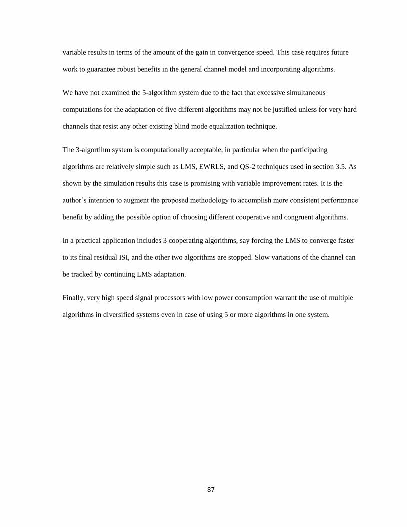
87
variable results in terms of the amount of the gain in convergence speed. This case requires future
work to guarantee robust benefits in the general channel model and incorporating algorithms.
We have not examined the 5-algorithm system due to the fact that excessive simultaneous
computations for the adaptation of five different algorithms may not be justified unless for very hard
channels that resist any other existing blind mode equalization technique.
The 3-algortihm system is computationally acceptable, in particular when the participating
algorithms are relatively simple such as LMS, EWRLS, and QS-2 techniques used in section 3.5. As
shown by the simulation results this case is promising with variable improvement rates. It is the
author’s intention to augment the proposed methodology to accomplish more consistent performance
benefit by adding the possible option of choosing different cooperative and congruent algorithms.
In a practical application includes 3 cooperating algorithms, say forcing the LMS to converge faster
to its final residual ISI, and the other two algorithms are stopped. Slow variations of the channel can
be tracked by continuing LMS adaptation.
Finally, very high speed signal processors with low power consumption warrant the use of multiple
algorithms in diversified systems even in case of using 5 or more algorithms in one system.
88
3.7 References
[1] Clarkson, P.M., “Optimal and Adaptive Signal Processing,” CRC Press LLC, 1993.
[2] Ding, Z.Z., Zhang, X.D., Su, Y.T., “Performance Analysis of Nested RLS-Type Interference
Suppression Algorithm for CDMA System in Dispersive Channels,” IEEE Signal Processing
Letters, Vol. 14, No. 1, January 2007.
[3] Hayes, M.H., “Statistical Digital Signal Processing and Modeling,” John Wiley & Sons,1996.
[4] Kumar, R., Moore, J.B., “Adaptive Equalization via Fast Quantized State Method”, IEEE
Transactions on Communications, Vol. COM-29, No. 10, October 1981.
[5] Kumar, R., Khor, K. “Adaptive Decision-Directed Quantized-State Algorithms for Multi-user
Detection of CDMA Signals,” IEEE Aerospace Conference, 2007.
[6] Therrien, C.W., “Discrete Random Signals and Statistical Signal Processing,” Prentice-Hall,
1992.
[7] Widrow, B., Stearns, S.D., “Adaptive Signal Processing”, Prentice-Hall, New Jersey, 1985.
[8] Widrow, B, Walach, E., “Adaptive Inverse Control: A Signal Processing Approach,” Wiley-
IEEE Press, Nov. 2007.

89
Chapter 4: Neural Networks, a Novel Back Propagation Configuration for Wireless
Channel Equalization
4.1 Introduction
Neural networks are viewed as dense interconnections of elementary computational elements
known as perceptrons that are simplified models of neurons in the human brain. This model is based
on our perception and understanding of the biological nervous system. Neural networks also have
been considered as massively parallel networks composed of many computational elements
organized in parallel to each other and in turn cascaded to other elements in different layers. Almost
every introduction to neural networks includes a simplified nervous anatomy to demonstrate the
resemblance to the human brain.
Neural nets have great potential applications in the area of speech processing and pattern recognition
and multi-dimensional signal processing. These applications usually seek high parallelism and high
computational costs. In recent years the technique of neural nets has been applied to other
engineering problems including, but not limited to, wireless channel equalization and adaptive
control.
Although there are early traces of neural nets in the literature by Widrow (1962) and Stark, et.al.
(1962), the pioneering works by Rosenblatt (1962) deserve the distinction of being the first formal
analysis of what was called perceptron analysis. These are actually adaptive linear combiners
augmented by a nonlinear function block (See Figure 4-1.) Grossberg (1976) and later Carpenter and
Grossberg (1983) developed adaptive resonance theory and the architecture that became known as
self-organizing neural nets for pattern recognition. Hopfield (1982) created Hopfield models for the
class of recurrent (feedback) networks, which in combination of an algorithm called back
propagation demonstrated significant success in some applications. The development of the early
neural network systems was taking place at the same time that other adaptive signal processing

90
algorithms, in particular the attractive LMS algorithm, were successfully applied to many scientific
and engineering problems (See Widrow and Stearns (1985)). Some disappointing experiences with
this new concept (in addition to the fact that efforts to develop learning rules for neural networks
with multiple layers were not successful) led to a conundrum in the research of this area for about a
decade. Particularly, Minsky and Selfridge (1961) showed the inadequacy of perceptron methods, or
more generally the single-layer network in cases where linear classifications were not possible. They
suggested the use of Multi-Layer Perceptrons (MLP) that has nonlinear behavior. Minsky also gave a
treatment of the subject in his 1969 textbook.
Σ
uv
w1
w2
wL
w0
bias
activity
Activation
function
z1
z2
zL
Figure 4-1 Basic perceptron architecture
So far, most neural nets have feed forward classifier architecture. A major advancement was made
by Werbos (1974). Werbos proposed a back propagation learning algorithm which has become the
most applied algorithm in many applications of neural nets including the signal processing
application. His work remained unknown until Parker (1985) revitalized the back propagation
algorithm in his MIT report. After the works by Parker and many others, the multilayer neural nets
with some modifications to the architecture and the choice of activation function using back
propagation have gained momentum in the research community. Specially, it has been employed for
problems of channel equalization and system identification (see Botoca and Budura (2006), Chang,

91
et.al. (2010), Chen and Mars (1991), Fang and Chow (1999), Feng, et.al. (2003), Kechriotis, et.al.
(1994), Lee and Kim (2003), Li and Er (2008), Mo and Shafai (1994), Rui, et.al. (1999), Sarajedini
and Hecht-Nielson (1992), Satapathy and Subhushini (2009), Xie and Leung (2005), and Zhang,
et.al. (2010)).
Rumelhart, et.al. (1985, 1986) introduced the use of sigmoid function ( )
in place of the
signum function ( ( )) that also was known as slicer or hard-limiter to modify the nonlinear
activation. Overall, the idea of the combination of this back propagation learning algorithm with
multilayer architecture has demonstrated great achievements in many applications.
We conclude this section by briefly mentioning some of the salient advantages of neural nets as
compared to general linear adaptive filtering.
The first advantage of neural nets is obviously their massive parallel distributed structure that affords
the network strong computing power. The second and unique advantage is what is known as
generalization by which the neural nets are capable of learning. In simple words, a trained network
can generate reasonably correct and expected outputs for the inputs that have not been encountered
during the training process. Consequently, neural nets are capable of solving relatively complicated
problems. In some large and hard-to-attack problems several networks are deployed, each having a
specific task to perform, so that an appropriate structure for each network can be selected and
configured.
Haykin (2009) has summarized the important features of common neural networks that are concisely
given in the following.
Nonlinearity: nonlinearity is the prominent feature of neural nets. Although a neural net
can also be linear in design; however its distributed nonlinearity is used almost exclusively
in most of the applications. In passing, we mention that nonlinear channels cannot be

92
equalized adequately by a linear equalizer, and the neural net has becomes an essential
option.
Input-output mapping: supervised learning that is performed in adjusting the synaptic
connection weights by applying a set of training inputs or examples, and computing the
network error using the knowledge of the desired (expected) response. If a sufficient number
of training inputs is exploited, and if the synaptic weights have reached stable and stationary
values, we can say that the network has created an input-output mapping for the problem
under investigation. It is an outstanding feature that unlike almost all other channel
equalization methods no statistical assumptions about the possible input set are made.
Adaptivity: neural nets have the capability to adapt their synaptic weights according to
changes in the environment or inputs. Specifically, they can be retrained to perform an
ongoing adaptation to respond to minor changes encountered.
There are other features such as fault tolerance and many more that will not fit in a concise
introduction.
4.2 Fundamental Theory of Neural Networks
The credit for introducing the neural networks as we know them today goes to McCulloch and Pitts
(1943) when they designed a simple model they called “neuron”. Nonetheless, the Rosenblatt
perceptron (1958) became the main building block for various classes of neural networks that were
designed and investigated in the second half of the last century.
The perceptron is a simple network similar to what is known as a linear combiner except for the
addition of a constant input called bias and hard-limiter (signum function). The latter was replaced
with other nonlinear functions such as sigmoid or hyperbolic tangent, etc. designated here by ( ) in
different configurations and applications (see Figure 4-2).

93
The formulation by which the perceptron output is computed is a simple summation sometimes
referred to as activity , and the application of a nonlinear function. These are given in the following
equations for the epoch or step (as the perceptron is being trained adaptively):
[ ] ∑ [ ]
( )
[ ] ( [ ]) ( )
Σ φ (.)
uv
w1
w2
wL
w0
b
activity
Activation
function
z1
z2
zL
Figure 4-2 The perceptron architecture with general nonlinear activation function
Rosenblatt developed the learning algorithm to adjust (adapt) the free parameters that comprise the
weights for what are called synaptic connections for a perceptron with L
connections. An extra parameter can be used for the bias input connection that is usually constant
with in many designs. The bias is not always included as it might not be necessary for the
perceptron performance and can be eliminated in certain applications.
This model was originally applied to the problem of classification of patterns, and so they were also
called classifiers. They were proved to be successful in pattern classification when the sets of
different patterns were linearly separable, say by a straight line in two-dimensional space or by a
hyperplane in L-dimensional space. Rosenblatt (1962) provided the well-known “perceptron

94
convergence theorem” that is also given by others with minor changes (see Haykin (2009), pp. 50).
The simple perceptron equation consists of a linear combination of inputs or stimuli and the bias
that together generate activity ∑ [ ] . In the simple form the perceptron separates
two classes of the stimuli by a hyperplane with the simple equation:
∑
( )
The final decision in early perceptron applications was made by using a hard-limiter ( ).
The synaptic weights of the perceptron can be iteratively adapted. The adaptation like any other
adaptive algorithms requires first a method of computing the output error and then a method to make
an appropriate correction to the weights according to the computed error.
It is the method designed for these two steps that creates many successful advanced network
architecture and algorithms. The perceptron created on a single neuron has a very limited
performance domain. It can separate only two linearly separable classes and is not capable of
implementing more complicated and nonlinear functions. The network should be expanded to
comprise more neurons and more layers containing similar neurons.
The natural option for further examination of neural network performance was to expand the
network to employ more neurons and more layers comprising many more neurons. Additional
neurons bring the capability to separate more classes (more than two) and the additional layers
seemingly removes the linear separability constraint. Benefits come with the cost of more
computation in addition to the complexity of error and correction formulation. The use of sigmoidal
function ( )
and hyperbolic tangent ( )
were investigated in literature as the
activation functions replacing hard limiter or threshold ( ) ( ).

95
4.3 Network Architectures and Algorithms
In common neural network architectures, the neurons are grouped in the form of layers. Neurons in
the same layer usually share the same set of inputs or stimuli. Networks with only one layer are
known as single-layer feed forward (see Figure 4-2). Each neuron in the same layer generates an
output, together these outputs can be applied to another layer of neurons as stimuli, and thus creating
a two-layer feed forward networks. In general, adding more layers in general creates multilayer feed
forward networks (see Figure 4-3). If the final outputs of the network are fed back to the network
input layer the new configuration is known as recurrent (see Bradley and Mars (1994 and 1995)). It
also justifies the ‘feed forward” modifier for non-recurrent networks.
Important parameters and features that distinguish the modern neural net architectures are the choice
of activation function ( ), the rule by which the output error in each step or epoch [ ] is
determined, and the corresponding correction applied to the weights in each layer in an adaptive
method. The networks are divided into two categories based on the output error calculations,
supervised nets in which the exact required or expected output is available to the network, and
unsupervised or blind nets when this information is not available. The present neural network
architectures applied to the channel equalization problem are similar to those typically used in
various other applications in the spirit of the theorem by Hecht-Nielson (1987) that states: “Any
continuous function in a closed interval can be approximated by back propagation neural network
with one hidden layer.”

96
Σ φ1(.)
u1v1
w11
w12
w1N
w0
z1
z2
zN
Σ φ1(.)
wN1
wN2
wNN
w0
vNuN
b1
Σ φ0(.)f1
u2
Σ φ0(.)
b1
b2
b3
f2
g1
g2
Input layer
Output layer
θ11
θ12
θMN
θM1θ1N
Figure 4-3 A multilayer perceptron example of two layer model with N neurons in the input
and M neurons in the output layer
The Back Propagation Algorithm
One major reason for the popularity of adaptive supervised training of multilayer perceptrons or
neural nets in general is the development of back propagation algorithm on recurrent networks. The
development of back propagation algorithm is credited to Rumelhart and McClelland (1986) in their
book “Parallel Distributed Processing”. Their development has thwarted the Minsky and Papert
(1969) argument of multilayer networks deficiency.
Based on the back propagation algorithm the network operates in two major phases. Phase one is
forward propagation in which the ultimate output error of the current step is computed based on
current synaptic weight values in each layer from the very input of the network layer-by-layer toward
the output. In second phase or back propagation the gradient of error surface with respect to weights
in each layer is computed from the output of the network backward toward the input layer and is

97
used for updating the weights of each neuron synaptic connections in each layer. This is also the
kernel of what we know as stochastic approximation (see chapter 2). It can be said that the success of
the back propagation method has revitalized the study and application of neural networks.
Radial-Basis Function Networks
Cover’s theorem (1965) is often referred to as the incentive for designing multi-layer neural
networks for the case of classes that are not linearly separable. This is in fact a different approach
compared to back propagation for solving the classification problem of nonlinearly separable
patterns. The two phase operations are modified so that in the first a transformation is adopted to
convert a set of nonlinearly separable patterns into a possibly linearly separable set. The justification
for this attempt is supported by the Cover’s theorem. The second phase is dedicated to find the
solution to the problem in the least-squares sense.
The radial-basis functions (RBF) are used for the nonlinear transformation for the sets that possess
spherical symmetry in relatively high-dimensional inputs and hidden layer networks.
The RBF are the functions that have spherical symmetry are generally in the form of (‖ ‖ )
for , when are the inputs to the network and the corresponding activation
function
( ) ∑ (‖ ‖ )
( )
The Gaussian function ( ) (‖ ‖ ) is often tested in many applications (see for
examples Botoca and Budura (2006), Sarajedini and Hecht-Nielson (1992)).

98
Self-Organizing Maps
Like many other advanced neural nets, self-organizing nets are also employed in pattern recognition
and image processing. These nets bear some resemblance to the human brain in sensory systems. The
self-organizing map is based on a technique known as competitive learning. There is only one
winner neuron of the output layer or other groups of neurons in competitive learning. The winner
neuron will be relocated topologically in an ordered manner with respect to other neurons in the
same layer.
The concept of neural network has explored many regions of adaptive systems and learning
processes.
There are more versions of networks that are not mentioned in this chapter, each demonstrating some
advantages in certain applications. The use of fuzzy logic in neural nets for example has received
special attention and several research documents have been published for this case (see Kosko’s
book (1992): Neural Networks and Fuzzy Systems).
4.4 A Novel Neural Network as a Wireless Channel Equalizer
There are many research papers that agree on the fact that linear transversal equalizers are
not capable of equalizing highly nonlinear channels. Gibson et.al (1989) has explicitly mentioned
that: “When the channel is non-minimum phase, the decision boundary of equalizer is highly
nonlinear and deviates markedly from any decision boundary which can be formed by a linear
transversal equalizer.”
In searching for a neural network architecture suitable for equalizing an unknown wireless channel a
reasonable choice would be a multi-layer network and the use of the back propagation algorithm in a
common gradient descent adaptation.

99
The baseband binary data channel models with the assumptions in chapter 2 are considered. The
hyperbolic tangent activation function is adequate for binary data system and the bias input
connection in each neuron is eliminated.
We decided to try supervised training with the hope of obtaining very fast convergence and
significant reduction in the training period (see section 4.6), as blind training does not seem
promising in speed and simplicity (See Zhang, et.al. (2010), Xie and Leung (2005).)
Figure 4-4 shows the block diagram of the proposed neural network (Kumar and Jalali (2012)). As
shown in the figure, the sequence of symbols is input to an unknown channel. The output of the
channel is corrupted by noise. The noisy channel output is inputted to the neural network adaptive
equalizer through a tapped delay line of length M. The outputs of the tapped delay line are
segmented into a number of groups such that each adjacent group may possibly have some amount
of overlap among their elements with each group of the tapped delay line outputs connected to a
neuron. Thus the number of neurons and the total number of synaptic connections is dependent on
the length of the delay line, the amount of overlap among the various groups and the number of
elements in each group. The computational complexity is determined by the total number of synaptic
connections in the network and thus reduced overlap among the various groups’ results in relatively
reduced computational complexity but may possibly result in relatively reduced convergence rate.
Consequently, there may be a trade-off between t computational complexity and the rate of
convergence via the length of the tapped delay line M, the number of neurons S, and the number of
synaptic connections to each neuron L.
Each group of the delay line outputs along with its associated neuron has a structure similar to that of
a linear equalizer except that the nonlinear activation function operating in the neuron replaces the
decision function of the linear equalizer.
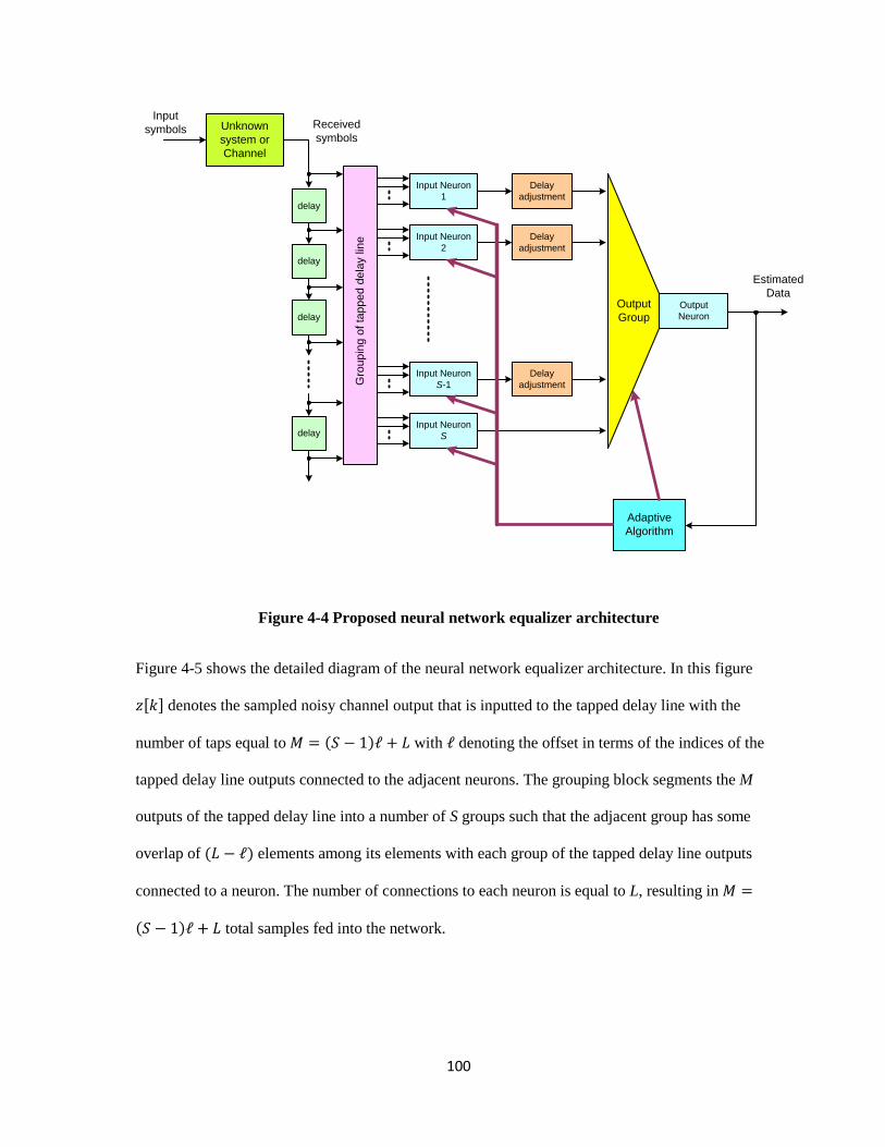
100
Unknown
system or
Channel
Input
symbols Received
symbols
Input Neuron
1
Input Neuron
2
Input Neuron
S
Input Neuron
S-1
Delay
adjustment
Delay
adjustment
Delay
adjustment
Estimated
Data
Adaptive
Algorithm
Output
Neuron
delay
delay
delay
delay
Output
Group
Gro
up
ing
of ta
pp
ed
de
lay lin
e
Figure 4-4 Proposed neural network equalizer architecture
Figure 4-5 shows the detailed diagram of the neural network equalizer architecture. In this figure
[ ] denotes the sampled noisy channel output that is inputted to the tapped delay line with the
number of taps equal to ( ) with denoting the offset in terms of the indices of the
tapped delay line outputs connected to the adjacent neurons. The grouping block segments the M
outputs of the tapped delay line into a number of S groups such that the adjacent group has some
overlap of ( ) elements among its elements with each group of the tapped delay line outputs
connected to a neuron. The number of connections to each neuron is equal to L, resulting in
( ) total samples fed into the network.
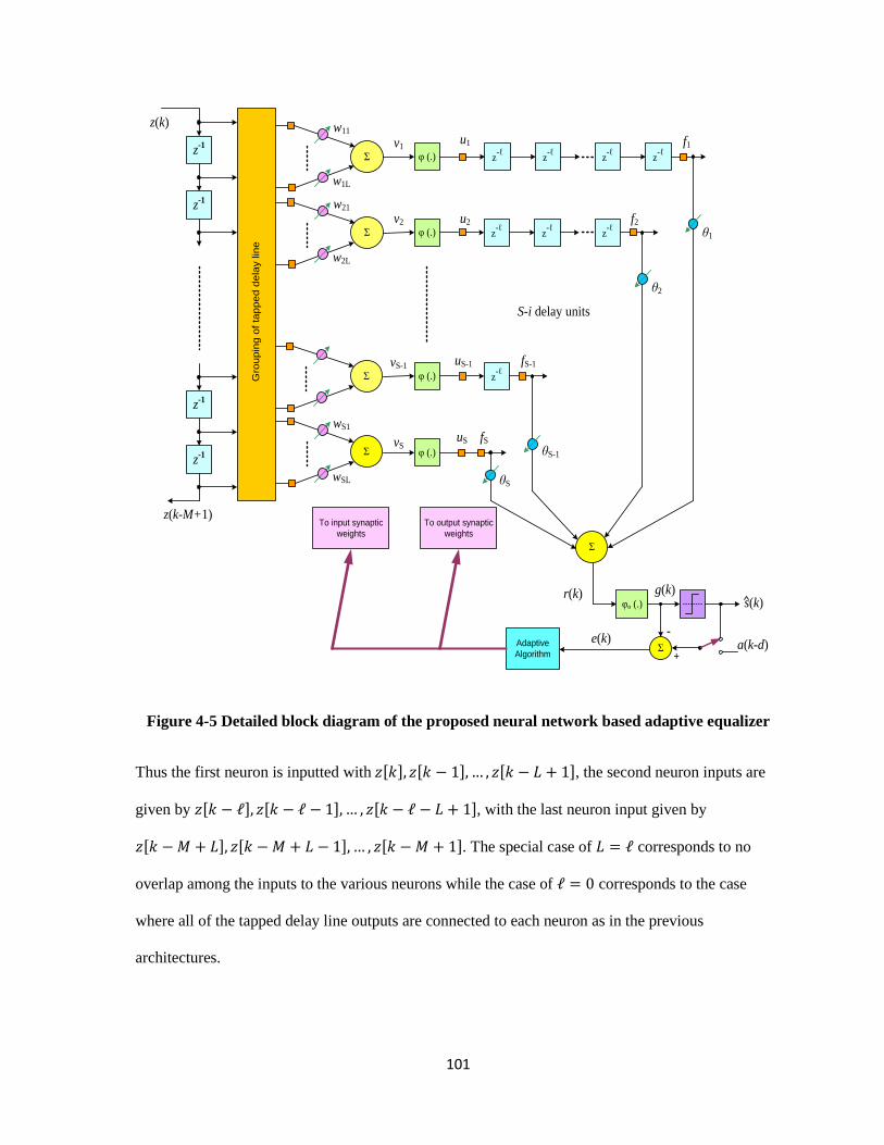
101
z-1
z-1
z-1
z-1
Σ
Σ
Σ
φ (.)
φ (.)
φ (.)
Σ φ (.)
z-ℓ
z-ℓ
z-ℓ
z-ℓ
z-ℓ
z-ℓ
z-ℓ
z-ℓ
φo (.) s(k)
z(k)
r(k) g(k)
Σ a(k-d)Adaptive
Algorithm
e(k)
+
-
u1
u2
uS-1
uS
fS-1
fS
f1
f2
w11
θS
θS-1
θ2
θ1
vS-1
vS
v1
v2
z(k-M+1)
S-i delay units
Σ
w1L
w21
w2L
wS1
wSL
Gro
up
ing
of ta
pp
ed
de
lay lin
e
To input synaptic
weights
To output synaptic
weights
Figure 4-5 Detailed block diagram of the proposed neural network based adaptive equalizer
Thus the first neuron is inputted with [ ] [ ] [ ], the second neuron inputs are
given by [ ] [ ] [ ], with the last neuron input given by
[ ] [ ] [ ]. The special case of corresponds to no
overlap among the inputs to the various neurons while the case of corresponds to the case
where all of the tapped delay line outputs are connected to each neuron as in the previous
architectures.

102
In terms of the computational complexity of the proposed equalizer, the number of neurons S in the
input layer is given by
. Thus, for a selected length of the delay line M and the number
of inputs L to each neuron, the number of neurons S is minimized by maximizing the offset .
From the results for the linear equalizer it is known that the performance in terms of the residual ISI
is increased with an increase in M. Thus, intuitively increasing M would also result in increased
performance of the neural network-based equalizer. Also, it is expected that a higher value of L
would result in better performance. Although the performance will also depend upon the number of
neurons S, the dependence of the performance on S will be relatively less when every neuron is
processing all or most of the inputs. The number of synaptic connections in the first layer is given by
( ) (
) and is equal to M for . In comparison to this, in previous neural network
equalizer architectures, the number of neurons is selected independently of M; thus the number of
synaptic connections is equal to showing at least in intuitive terms that the proposed
architecture can have much less computational requirements for similar level of performance.
Moreover, the previous neural network based equalizer architectures also have hidden layers of
neurons that further increase the computational requirements. The proposed architecture does not
have any hidden layer. In the proposed architecture, the absence of hidden layer is compensated by
the introduction of delay adjustments in the outputs of the neurons in the first layer before being
connected to the output neuron. The functions ( )in Figure 4-5 may be the sigmoidal, hyperbolic
tangent or any other similar function.
As shown in Figure 4-5, the neuron output is delayed by ( ) samples for .
Each group of delay line outputs (along with its associated neuron) has a structure similar to that of a
linear equalizer, except that the nonlinear function operating in the neuron replaces the decision
function of the linear equalizer. Thus the output of the S neurons may be considered to be different
versions of the equalized output, except that there is a relative delay among the various outputs. This

103
is in view of the fact that the inputs to the other neurons are the delayed versions of each other.
Therefore as shown in Figure 4-5, with an introduction of the appropriate delays among the output to
various neurons, the relative delays introduced by the input tapped delay line are equalized and the
various neuron outputs have a cumulative effect, achieving a similar effect when different neurons
all are inputted with exactly the same inputs but with much reduced computational complexity. As
shown in Figure 4-5, the delayed versions of the outputs of the neurons in
the input layer are inputted to the single neuron in the output layer with weights . The
output [ ] of the neuron in the output layer is input to the decision device whose output [ ] is
equal to ( [ ]) with ( ) denoting the signum function. During the initial training phase, the
equalizer error signal is [ ] [ ] [ ] where [ ] denotes the symbol at the input of the
channel and denotes the sum of delays introduced by the channel and the equalizer. After the
initial phase, [ ] is replaced by [ ] as shown in Figure 4-5. The equalizer error [ ] is input
to the adaptive algorithm block that updates the weights of the various neurons in the neural network
adaptive equalizer. Section 4.5 describes the adaptive learning algorithm for the neural network.
4.5 Learning Algorithm
For the neural network of Figure 4-5, the nonlinear activity function ( )is selected to be the
hyperbolic tangent function ( ). The equations for the forward propagation of the signal through
the network are derived for this activity function. The back propagation algorithm is used to
determine the local and complete gradients required for updating the input and output layer synaptic
weights as given in the following sections.

104
Forward propagation
Forward propagation can be performed by starting to compute the activation functions of the input
layer neurons, each having weighted synaptic connections. At the iteration or epoch of the
adaptive algorithm, one obtains:
[ ] ∑ [ ] [ ( ) ]
( )
The appropriate activation function employed is the hyperbolic tangent function, thus the outputs
( ) of the neurons in the input layer are given by:
[ ] ( [ ]) ( )
As may be observed from Figure 4-5 there is no bias or input threshold present for any neuron in the
input and output layers of the network. The outputs of the first layer are delayed so that they convey
the information about the channel and the data symbols that belong to the same time slot, in other
words they are adjusted to be concurrent with respect to the output of the farthest (most delayed)
neuron in the input layer. These delayed outputs are computed as follows.
[ ] [ ( ) ] ( )
The signals [ ] [ ] [ ] are inputted to the output layer that possesses only one neuron. It
may be observed that no hidden layer is incorporated in the neural network of Figure 4-5. The output
layer activity is computed as [ ] ∑ [ ] [ ] and using the same activation function as for
the input layer. Thus the output of the neural network is obtained by [ ] ( [ ]) .
The final estimate for the case of binary data [ ] sgn( [ ]) is the estimate of the channel
delayed input [ ], i.e., when appropriately converged in supervised mode [ ] [ ] and the
error [ ] is applied for the learning algorithm and is given by:

105
[ ] [ ] [ ] in training mode,
[ ] [ ] [ ] in decision-feedback mode.
The weights of the various synaptic connections in the network are iteratively adjusted on the basis
of the error [ ] using the back propagation algorithm as follows.
Back propagation: Output layer
The objective function for optimization of the equalizer performance is defined as [ ]
{ [ ]}
where [ ] [ ] [ ] is the estimation error and represents expectation. Notice that in the
short training mode [ ] [ ] [ ] is the actual error.
The computation of the total gradient for the update equations of the output layer weight vector is
summarized in the following:
[ ]
{ [ ]
[ ]
} ( )
The application of the output local gradient denoted by that is defined in the following simplifies
the equation for complete gradients:
[ ] [ ]
[ ]
[ ]
[ ] ( )
[ ]
[ ]
[ ]
[ ]
[ ]
[ ]
( ) ( ) ( )
The local gradient for the output neuron is computed as
[ ] ( [ ]) ( [ ]) ( )
Therefore the stochastic gradient algorithm for updating synaptic weights of the output layer is:
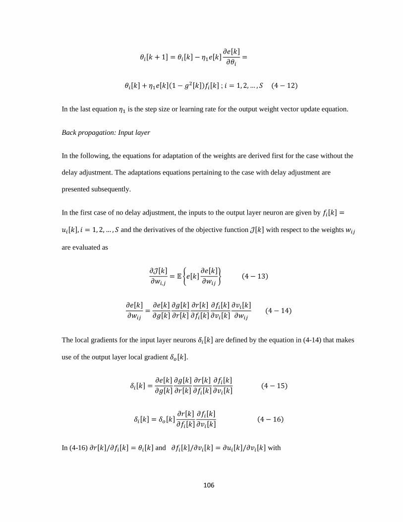
106
[ ] [ ] [ ] [ ]
[ ] [ ]( [ ]) [ ] ( )
In the last equation is the step size or learning rate for the output weight vector update equation.
Back propagation: Input layer
In the following, the equations for adaptation of the weights are derived first for the case without the
delay adjustment. The adaptations equations pertaining to the case with delay adjustment are
presented subsequently.
In the first case of no delay adjustment, the inputs to the output layer neuron are given by [ ]
[ ] and the derivatives of the objective function [ ] with respect to the weights
are evaluated as
[ ]
{ [ ]
[ ]
} ( )
[ ]
[ ]
[ ]
[ ]
[ ]
[ ]
[ ]
[ ]
[ ]
[ ]
( )
The local gradients for the input layer neurons [ ] are defined by the equation in (4-14) that makes
use of the output layer local gradient [ ].
[ ] [ ]
[ ]
[ ]
[ ]
[ ]
[ ]
[ ]
[ ] ( )
[ ] [ ] [ ]
[ ]
[ ]
[ ] ( )
In (4-16) [ ] [ ] [ ] and [ ] [ ] [ ] [ ] with

107
[ ]
[ ] [ ]
[ ] ( )
Thus
[ ]
[ ]
[ ] ( )
Substitution of (4-18) in (4-16) results in
[ ] [ ] [ ]( [ ]) ( )
The last term in (4-14) is given by
[ ]
[ ( ) ] ( )
The Equation (4-20) follows directly from (4-5). With the substitution of (4-16) to (4-20) in (4-14),
one obtains the derivative of [ ] with respect to as:
[ ]
[ ] [ ](
[ ]) [ ( ) ] ( )
For and .
Further, the output layer local gradient from (4-9) is given as:
[ ] ( [ ]) ( )
With the proposed delay adjustments the input signals to the output layer neuron are given by
[ ] [ ( ) ] for . One starts with the following equation:
[ ]
[ ]
[ ]
[ ]
[ ]
[ ]
[ ]
( )

108
In (4-23) ( ) . Similar to the first case of no delay adjustments, in this case one also
obtains [ ] [ ] [ ] for the first partial derivative on the right hand side of (4-23). The
other partial derivatives in (4-23) are taken as follows:
[ ]
[ ] [ ( ) ]
( ( ) ) ( ) ( )
[ ]
[ ( ) ( ) ] [ ( ) ] ( )
It may be noted that the last expression in (20) is independent of input layer neuron index , and this
independence can make the computations somewhat faster. Substitution of (4-24) and (4-25) in
Equation (4-23) yields:
[ ]
[ ] [ ](
[ ]) [ ( ) ] ( )
The stochastic gradient based update equations for adjustment of the synaptic weights for the input
layer neurons may be generally written as:
[ ] [ ] [ ] [ ]
( )
The use of (4-26) in Equation (4-27) results in the following adaptive algorithm for the adjustment of
the weights of the synaptic connections of the input layer in the neural network:
[ ] [ ] [ ]( [ ]) [ ](
[ ]) [ ( ) ] ( )
For . In (4-28) the constant is the step size or learning rate for input
layer neurons.
The simulation results of the following section show that not only the update formula (4-28) is
somewhat faster because each update equation includes the same input symbol set due to the

109
independence from the neuron index , but also it makes a very significant difference in the
convergence time for all the channels considered for simulations.
4.6 Performance and Simulation Results for the Proposed Network
In order to evaluate the performance of the neural network equalizer of section 4.4, three different
non-minimum phase channels are examined. These channels have been used in the previously
published literature and are considered to be more difficult to equalize. The performance is evaluated
in terms of the mean square error (MSE) computed by a simple average of the square of the true
equalization error [ ] [ ] [ ] over a moving window of size 50.
The first simulated channel has the impulse response:
[ ]
with norm ‖ ‖ . The corresponding transfer function is given by:
( )
The transfer function in this case has zeros located at with
the phases shown in degrees. Only 40 steps or epochs are used for training including the delay, the
input layer is selected to have neurons, each having synaptic connections, the offset
, and the symbol bit energy to noise spectral density ratio
. The step sizes for the
input and the output layer adaptations are , that are changed to after
the initial convergence, the overall network delay between the network estimate and the channel
input data is set to .

110
Figure 3 shows the instantaneous actual error [ ] from the very beginning of the transmission.
The first 14 network data estimates [ ] of the network have not been used due to the overall delay
of the channel and the network. Note however that the azimuth axis for Figures 3–6 show the
number of symbols including those in the delay period of 14 symbols.
Figure 4-6 Instantaneous error (top) and the bit errors that have occurred during the
adaptation process (bottom).
Figure 4-6 indicates the mean square error for this channel simulation over a period of the first 1000
iterations.
There are only a total of 6 bit errors in the whole process. The data bit error figure is zoomed in to
the first 100 steps because no further bit error occurs for another 2000 bits of data exchanged. Figure
4-7 plots the mean squared error plotted over a period of first 1000 bits.
0 100 200 300 400 500 600 700 800 900 1000
-1
0
1
Err
or
eT (
k)
Instantaneous error eT
(k)
20 30 40 50 60 70 80 90 100
-2
-1
0
1
2
Time index k
Err
or
es (
k)
The error es (k)

111
Figure 4-7 Mean Square Error (MSE) averaged over a moving window of 50 steps
The second channel has been taken from Bradley and Mars (1995) and the impulse response of the
channel is [ ] with norm ‖ ‖ .
The corresponding transfer function is given by:
( )
The transfer function has zeros located at ; and thus the transfer
function is of composite minimum and non minimum phase type.
In this case 80 steps or epochs have been used for training including the delay; the input layer is
selected to have neurons, each having synaptic connection weights, the offset ,
and the symbol bit energy to noise spectral density ratio is
. The step sizes for the input
and output layer adaptations are , that are changed to after
convergence; the overall network delay between the network estimate and the channel input data is
set to .
Figure 4-8 shows the instantaneous actual error [ ] from the start of the transmission and the data
error that occurred from the very beginning of the transmission. Obviously the first 15 network data
0 100 200 300 400 500 600 700 800 900
0
0.2
0.4
0.6
0.8
1
Mean Square Error of the data estimate
Time index k
MS
E

112
estimates [ ] of the network have not been used due to the overall delay. Figure 4-9 plots the mean
square error for this case.
Figure 4-8 Instantaneous error (top) and the only bit errors that have occurred during the
adaptation process (bottom).
Figure 4-9 Mean Square Error (MSE) averaged over a moving window of 50 steps
0 100 200 300 400 500 600 700 800 900 1000-2
-1
0
1
2
Instataneuos error eT
(k)
Err
or
e T (
k)
20 30 40 50 60 70 80 90 100
-2
-1
0
1
2
The error es (k)
Time index k
Err
or
e s (k
)
0 100 200 300 400 500 600 700
0
0.2
0.4
0.6
0.8
1
1.2
Mean Square Error of the data estimate
Time index k
MS
E
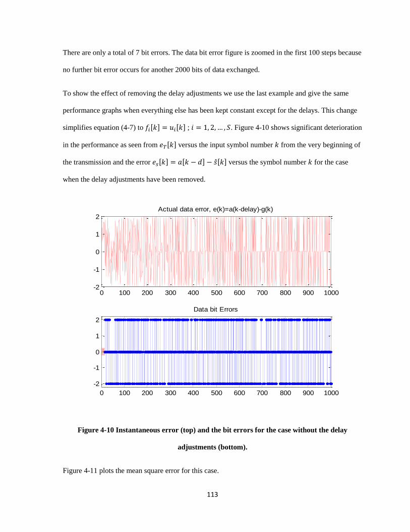
113
There are only a total of 7 bit errors. The data bit error figure is zoomed in the first 100 steps because
no further bit error occurs for another 2000 bits of data exchanged.
To show the effect of removing the delay adjustments we use the last example and give the same
performance graphs when everything else has been kept constant except for the delays. This change
simplifies equation (4-7) to [ ] [ ] ; . Figure 4-10 shows significant deterioration
in the performance as seen from [ ] versus the input symbol number from the very beginning of
the transmission and the error [ ] [ ] [ ] versus the symbol number for the case
when the delay adjustments have been removed.
Figure 4-10 Instantaneous error (top) and the bit errors for the case without the delay
adjustments (bottom).
Figure 4-11 plots the mean square error for this case.
0 100 200 300 400 500 600 700 800 900 1000-2
-1
0
1
2Actual data error, e(k)=a(k-delay)-g(k)
0 100 200 300 400 500 600 700 800 900 1000
-2
-1
0
1
2
Data bit Errors

114
Figure 4-11 Mean Square Error (MSE) without the delay adjustments
Increasing the training period to 100 data bits or steps will still result in a converged equalizer as
shown in Figure 4-12. It seems that the delays have shortened the training period for this example.
Figure 4-12 Instantaneous error (top) and the bit errors (bottom) for the case without the delay
adjustments after increasing the training period from 40 to 100 steps.
0 100 200 300 400 500 600 700 800 900 10000.8
1
1.2
1.4
1.6
1.8
2
2.2
2.4
2.6
2.8
Mean Square Error of the data estimate (dB)
epoch index
0 100 200 300 400 500 600 700 800 900 1000-2
-1
0
1
2Actual data error, e(k)=a(k-delay)-g(k)
50 100 150 200 250
-2
-1
0
1
2
Data bit Errors

115
The third channel has been used by Chang, Yang, and Ho [17] and has the impulse response
[ ] with norm ‖ ‖ .
The corresponding transfer function is given by
( )
The final channel is created by the sum ( ) ( ) ( ) with ( ) given by the above
equation. Thus the final transfer function turns out to be:
( )
The transfer function zeros are located at and have relatively wide
distribution in magnitude. In this case 80 steps or epochs have been used for training including delay;
the input layer is selected to have neurons, each having synaptic connection weights,
the offset , and the symbol bit energy to noise spectral density ratio is
. The step
sizes for the input and output layer adaptations are , that are changed to
after initial convergence; the overall network delay between the network estimate and the
channel input data is set to 16.
Figure 4-13 shows the instantaneous actual error among the channel input data and the network
output (to the decision device) [ ] and the data error that occurred from the very beginning of the
transmission. Obviously the first 16 data estimates [ ] of the network have not been used due to
the overall delay of the channel and the network.

116
Figure 4-13 Instantaneous error (top) and the only bit errors that have occurred during the
adaptation process (bottom)
There are only a total of 16 bit errors. The data bit error figure is zoomed-in for the first 100 steps
because no further bit error occurs for another 2000 bits of data exchanged. As may be deduced from
the simulation results presented here, the proposed equalizer architecture exhibits fast convergence in
all the cases considered for simulations. In all cases good convergence is achieved within 100
iterations and, except for the last case, convergence is achieved in about 25 iterations of the
algorithm.
Similarly, Figure 4-14 depicts the Mean Square Error in this case.
0 100 200 300 400 500 600 700 800 900 1000-2
-1
0
1
2
Instantaneous error eT
(k)
Err
or
e T (
k)
20 30 40 50 60 70 80 90 100
-2
-1
0
1
2
The error es (k)
Time index k
Err
or
e s (k
)

117
Figure 4-14 Mean Square Error (MSE) averaged over a moving window of 50 steps
We show the effect of removing the delay adjustments for the last example when all the other
parameters have been kept constant in the graphs of Figure 4-15. The instantaneous actual error
[ ] and the error [ ] [ ] [ ] are shown for this case.
Figure 4-15 Instantaneous error (top) and the data errors (bottom) versus iteration number k.
0 100 200 300 400 500 600 700 800 900
0
0.2
0.4
0.6
0.8
1
1.2
Time index k
MS
E
Mean Square Error of the estimate
0 100 200 300 400 500 600 700 800 900 1000-2
-1
0
1
2
Instantaneuos error eT
(k)
Err
or
e T (
k)
0 100 200 300 400 500 600 700 800 900 1000
-2
-1
0
1
2
The error es (k)
Time index k
Err
or
e s (k
)

118
The importance of the time adjustments for the network performance can be seen from the
significant increase in the number of data errors. Increasing the training steps to larger length did not
lead to convergence, that is, convergence could not be achieved without the delays for this channel.
In summary, we have shown that the proposed architecture and the introduction of the delay
adjustments have shortened the training period for some channels, and for harder channel examples
have made the convergence possible that otherwise could not be done with commonly used
configurations even with relatively long training periods. In fact, long training periods defy our goal
of making the equalization process efficient.
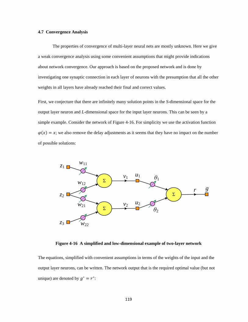
119
4.7 Convergence Analysis
The properties of convergence of multi-layer neural nets are mostly unknown. Here we give
a weak convergence analysis using some convenient assumptions that might provide indications
about network convergence. Our approach is based on the proposed network and is done by
investigating one synaptic connection in each layer of neurons with the presumption that all the other
weights in all layers have already reached their final and correct values.
First, we conjecture that there are infinitely many solution points in the S-dimensional space for the
output layer neuron and L-dimensional space for the input layer neurons. This can be seen by a
simple example. Consider the network of Figure 4-16. For simplicity we use the activation function
( ) ; we also remove the delay adjustments as it seems that they have no impact on the number
of possible solutions:
Σ
u1
w11
w12
z1
z2
v1
Σ
u2w21
w22z3
v2
Σ
g
θ1
r
θ2
Figure 4-16 A simplified and low-dimensional example of two-layer network
The equations, simplified with convenient assumptions in terms of the weights of the input and the
output layer neurons, can be written. The network output that is the required optimal value (but not
unique) are denoted by :
120
[ ] [
] [
] ( )
[ ] [
] [
] ( )
The network weights acting on the arbitrary set of triple inputs are:
[ ] [
] [ ] ( )
Now suppose a certain known solution is given by [ ], and we need to have
[ ] [ ] ( )
It can be seen that any of the equations , , and has many
pairs of solution that must be on the same curve in the parameters space. Replacing the activation
function with ( ) does not change this result as the hyperbolic tangent is a one-to-one
function.
According to this conjecture it is reasonable to assume that the space of the synaptic weights has
infinitely many solutions so that any random initial weight vector, with which the adaptation starts, is
in the neighborhood of one of the solution vectors and hence a local convergence condition suffices
for the network to take on one of the possible solutions. Moreover, the use of hyperbolic tangent
relaxes the convergence requirements as we show in the following.
In the case of binary data input there will be only two cases, the case that the actual and delayed data
input to the channel is [ ] (designated by Case + 1), and the case of [ ]
(designated by Case – 1). We consider these cases separately. Starting with the output layer synaptic
weights updates from Equation (4-12), we postulate that all of the parameters that are actually input
layer connection weights have already converged to their corresponding solution values:

121
[ ] [ ] [ ]( [ ]) [ ] ( )
[ ] [ ] [ ] ( )
[ ] [ ] [ ] ( )
Applying the actual (training mode) error to adaptation equation according to the back propagation
algorithm we obtain
[ ] [ ] ( [ ]) ( [ ]) [ ] ( )
[ ] [ ] ( [ ])( [ ]) [ ] ( )
Let the difference between the output layer weights and the exact local solution be denoted as
[ ] [ ] at the epoch. The last equations can be written in terms of [ ] as follows
(by subtracting from each side of the equation) .
[ ] [ ] ( [ ]) ( [ ]) [ ] ( )
[ ] [ ] ( [ ])( [ ]) [ ] ( )
When the network parameters and the corresponding functions have converged to a local solution
they settle at that point in the multidimensional space because either ( [ ]) or (
[ ]) in the adaptation equation for Case + 1 and – 1 respectively and no more adjustment will
be made to the parameters. This of course applies to the first layer outputs after delays namely
in Equation (4-37) and (4-38).
We need to compute network general output [ ] with the assumption that all other weights have
reached their local solution values except the one that is being analyzed, the weight in the single
output neuron [ ] [ ].
122
[ ] (∑ [ ] [ ]
) (∑
[ ] )
(∑
) ( [ ] )
(∑
) ( [ ] ) ( )
We have assumed that the adaptation has reached its local solution except for one parameter or
weight that is also assumed to be close to the solution point in the S-dimensional space. Based on
these assumptions it is fair to consider that | (∑
)| and | [ ] | .
Consequently, the following approximations are justified.
( [ ] ) [ ]
( )
(∑
)( [ ] ) [ ]
( )
(∑
)( [ ] ) [ ]
( )
Notice that keeping the second terms in Equation (4-41) and (4-42) leads to even smaller terms in the
adaptation equations due to the assumption | [ ] | (one can use approximations
and
to investigate this claim.) Inserting the approximations for the network output in
both cases we have:
[ ] (∑
) [ ]
(∑
) ( [ ] ) (∑
) [ ] ( )
We use the approximate network output in addition to (∑
) for Case + 1 and
(∑
) for Case – 1 in the adaptation equations as follows:

123
Case + 1: [ ] [ ] [ ] [ ]
[ ] [ ] ( [ ] ) ( [ ]
) ( )
[ ] [ ] [ ]
[ ]
( )
Case – 1: [ ] [ ] [ ] [ ]
[ ] [ ] ( [ ] )( [ ]
) ( )
[ ] [ ] [ ]
[ ]
( )
Finally, since the contribution of the misadjustment through tanh function to the network output
[ ] (∑
[ ] ) is by the factor [ ]
we multiply both sides of the equations
by to get:
[ ] [ ]
[ ]
[ ]
( )
[ ] [ ]
[ ]
[ ]
( )
Before checking the adaptation trend for each case it might be useful to looks at the hyperbolic
tangent function.
Figure 4-17 A graph of hyperbolic tangent function
-5 -4 -3 -2 -1 0 1 2 3 4 5-1.5
-1
-0.5
0
0.5
1
1.5
x
tan
h (
x)

124
Case + 1: First we modify Equation (4-47) to the following:
[ ] [ ]
( [ ] )
[ [ ]
] ( )
a) If [ ] then we have [ ]
[ ] because the second term in (4-49)
is positive. This helps by forcing [ ] (∑
[ ] ) closer to .
b) If [ ] that means its contribution is in the opposite direction, pushing [ ]
backward from . In this case the second term in (4-49) is still positive [ [ ] ]
because we assumed that | [ ] | . This updates the misadjustment in the correct
direction [ ] [ ]
that implies the output [ ] closer to Now if [
] it will follow the case a above, otherwise if [ ]
then the next change
[ ] [ ]
and the convergence continues in the correct direction.
Case – 1: Again we modify Equation (4-48) to the following
[ ] [ ]
( [ ] )
[ [ ]
] ( )
a) If [ ] then we have [ ]
[ ] because the second term in (4-50)
is negative ([ [ ] ] ). This helps by forcing [ ] (∑
[ ] )
to get closer to .
b) If [ ] that means that its contribution is in the opposite direction, pushing [ ]
backward from . The second term in (4-50) is still positive [ [ ] ] because we
assumed that | [ ] | . This updates the misadjustment in the correct direction that is
[ ] [ ]
that implies the output [ ] gets closer to Now if [
] it will follow the above, otherwise if [ ]
then the next change
[ ] [ ]
and the convergence continues in the correct direction.

125
The adaptation equations for the input layer neurons become complicated as their corresponding
gradients involve many free parameters. From Equation (4-28) for updating the weight of
synaptic connection of the neuron in the input layer we have the gradients as:
[ ] [ ]( [ ]) [ ](
[ ]) [ ( ) ] ( )
where [ ] [ ] for Case + 1, and [ ] ( [ ]).
Although there is a similar term in the gradient ( [ ]) having about the same relation to the
synaptic weights , a similar path of reasoning cannot follow because the similar assumption
| [ ]| | (∑ [ ] [ ( ) ] )| for nearly converged network cannot be
made. Moreover, the convergence of the output layer depends on the input layer convergence and not
the other way around.
It is the intention of the author to pursue possible approaches to the complete convergence analysis
of the proposed network or multilayer neural network in general in future research.

126
4.7 References
[7] Botoca, C., Budura, G., “Symbol Decision Equalizer using a Radial Basis Functions Neural
network”, Proc. of WSEAS International Conference on Neural networks, Cavtat, Croatia,
June 2006.
[8] Bradley, M.J., Mars, P., “A Critical Assessment of Recurrent Neural Networks as Adaptive
Equalizers in Digital Communications”, Application of Neural Networks to Signal Processing
(Digest No 1994/248), IEE Colloquium on.
[9] Bradley, M.J., Mars, P., “Application of Recurrent Neural Networks to Communication
Channel Equalization”, International Conference on Acoustics, Speech, and Signal Processing
(ICASSP), 1995.
[10] Carpenter, G.A., Grossberg, S., “A massively parallel architecture for a self-organizing neural
pattern recognition machine,” Computer Vision, Graphics, and Image Processing, Vol. 37,
1983, pp. 54-115.
[11] Chang, Y.J., Yang, S.S., Ho, C.L., “Fast Self-Constructing Fuzzy Neural Network-Based
Decision Feedback Equalizer in Time-Invariant and Time-Varying Channels”, IET
Communications, 2010, Vol. 4, Issue 4.
[12] Chen, J.R., Mars, P., “The Feasibility of Using MLP Neural Networks for System
Identification”, Neural Network for Systems: Principles and Applications, IEE Colloquium on,
1991.
[13] Fang, Y., Chow, T.W.S., “Blind Equalization of a Noisy Channel by Linear Neural Network”,
IEEE Transactions on Neural Networks, July 1999.
[14] Feng, J., Tse, C.K., Lau, F.C.M., “A Neural Network Based Channel Equalization Strategy for
Chaos-Based Communication Systems”, IEEE Trans. on Circuits and Systems, Vol. 50, No. 7,
July 2003.
127
[15] Gibson, G.J., Siu, S., Cowan, C.F.N., “Multilayer Perceptron structures applied to adaptive
equalizers for data communications”, Proc. ICASSP’89, May 1989.
[16] Grossberg, S., “Adaptive Pattern Classification and Universal Recording , II: Feedback,
expectation, olfaction, and illusions,” Bilog. Cybernetics, Vol. 23, 1976, pp. 187-202.
[17] Haykin, S., “Neural Network and Learning machines”, 3rd
Edition, Pearson Education, 2009.
[18] Hecht-Nielson, R., “Kolmogrov’s Mapping neural Network Existence Theorem”, IEEE
International Conference on Neural Network, Vol. 2, 1987.
[19] Hecht-Nielson, R., “The Theory of the Back propagation Neural Network”, International Joint
Conference on Neural Networks (IJCNN), 1989.
[20] Hopfield, J.J., “Neural networks and physical Systems with emergent collective computational
abilities,” Proc. Natl. Acad. Sci., Vol. 79, 1982, pp. 2554-2558.
[21] Jeffrey, A. “Handbook of Mathematical Formulas and Integrals,” 3rd
edition, Elsevier
Academic Press, 2004.
[22] Kechriotis, G., Zervas, E., Manolakos, E.S., “Using Recurrent Neural Networks for Adaptive
Communication Channel Equalization”, IEEE Trans. on Neural Networks, Vol. 5, No. 2, 1994.
[23] Kosko, B., “Neural Network and Fuzzy Systems,” Prentice-Hall, New Jersey, 1992.
[24] Kumar, R., Jalali, S.M., “Super Fast and Efficient Channel Equalizer Architecture Based on
Neural Network,” IEEE Conf. on Aerospace, March 2012.
[25] Lau, C., Editor, “Neural networks Theoretical Foundation and Analysis”, IEEE Press, 1992.
[26] Lee, C., Go, J., Kim, H., “Multigradient for Neural Networks for Equalization”, Systems,
Cybernetics and Informatics, Vol. 1, No. 3, 2003.
[27] Li, M.B., Er, M.J., “Channel Equalization Using Dynamic Fuzzy Neural Networks”, Proc. of
The 17th World Congress The International Federation of Automatic Control, Seoul, Korea,
July 2008.
[28] Lippman, R.P., “An Introduction to Computing with Neural Networks,” IEEE ASSP
Magazine, April 1987, pp. 4-22.

128
[29] McCullah, W.S., Pitts, W.,”A Logical calculus of the ideas immanent in nervous activity,”
Bulletin of Mathematical Biophysics, Vol. 5, 1943, pp. 115-133.
[30] Minsky, M.L., Papert, S.A., “Perceptrons,”, MIT Press, Cambridge, MA. 1969.
[31] Minsky, M.L., Selfridge, O.G., “Learning in random nets,” Information Theory, Fourth
London Symposium, London, Buttenvorths, 1961.
[32] Mo, S., Shafai, B., “Blind equalization using higher order cumulants and neural networks”,
IEEE Trans. Signal Processing, Vol. 42, No. 11, Nov. 1994.
[33] Parker, D., “Learning Logic”, Technical Report TR-47, Center for Computational research in
Economics and Management Science, MIT, Apr. 1985.
[34] Rosenblatt, F., “Principles of Neurodynamics: Perceptrons and the theory of brain
mechanisms,” Spartan Books, Washington DC, 1962.
[35] Rosenblatt, F., “The Perceptron: A Probablilistic model for information storage and
organization in the brain,” Psychological Review, Vol. 65, 1958, pp. 386-408.
[36] Rui, L., Saratchandran, P., Sundarajan, N., “Blind Equalization Using Higher Order Statistics
and Neural Networks: A Comparison Between Multilayer Feed Forward Network and Radial
Function Network”, Proc. of IEEE Signal Processing Workshop on Higher Order Statistics,
1999.
[37] Rumelhart, D.E., Hinton, G.E., Williams, R.J., “Learning internal representations by error
propagation,” ICS report 8506, Institute for Cognitive Sciense, University of California at San
Diego, La Jolla, CA, Sept. 1985.
[38] Rumelhart, D.E., Hinton, G.E., Williams, R.J., “Learning internal representations by error
propagation,” Parallel Distributed Processing, Vol. 1, Ch. 8, Cambridge, MA, MIT Press,
1986.
[39] Sarajedini, A., Hecht-Nielson, R., “The Best of Both Worlds: Casasent Networks Integrate
Multilayer Perceptron and Radial basis Functions”, International Joint Conference on Neural
Networks (IJCNN), 1992.
129
[40] Satapathy, J.K., Subhushini, K.R., “A Highly Efficient Channel Equalizer for Digital
Communication System in Neural Network Paradigm”, 2009 Conference on Innovative
Technologies in Intelligent Systems and Industrial Applications, July 2009.
[41] Veelenturf, L.P.J., “Analysis and Applications of Artificial Neural Networks”, Prentice Hall
International (UK), 1995.
[42] Widrow, B., Lehr, M.A., “30 years of Adaptive Neural Networks: Perceptron, Madaline, and
Backpropagation,” Proc. IEEE, Vol. 78, No. 9, Sept. 1990, pp. 1415-1442.
[43] Widrwo, B., “Generalization and information storage in network of Adaline neurons,” Self-
organizing Systems, Spartan Books, Washington DC, 1962, pp. 435-461.
[44] Widrow, B., Stearns, S.D., “Adaptive Signal Processing,” Prentice-Hall, New Jersey, 1985.
[45] Werbos, P., ”Beyond Regression: New Tools for Prediction and Analysis in the Behavioral
Sciences,” Ph.D. Thesis, Harvard University, Cambridge, MA, Aug. 1974.
[46] Xie, N., Leung, H., “Blind Equalization using a Perdictive Radial Basis Function Neural
Networks,” IEEE Trans. On Neural Networks, Vol. 16, No. 3, May 2005.
[47] Zhang, L., Liu, T., Sun, Y., Chen, L., “Research on Neural Network Blind Equalization
Algorithm with Structure Optimized by Genetic Algorithm”, IEEE Sixth International
Conference on Natural Computation (ICNC), 2010.
130
Chapter 5: Adaptive Simulated Annealing
5.1 Introduction
Every optimization problem should be based on minimization (or maximization) of a cost or
objective function, which usually is a function of a weight vector or state variable of many
dimensions. The weight vector needs to be adjusted to some optimum point in its space. The cost
function in the problem of channel equalization has several uncertainties associated with it (see
section 2.5 and Equation (2-19) and (2-20)). Other than the channel that is modeled by a linear
transversal impulse response with slow varying tap gains, there is channel noise and the desired
output that is unknown in the blind mode case. Furthermore, the cost function is normally
complicated. Let us assume the binary data input to the channel normalized to { } and the channel
that is considered fixed for the period of adaptation, then the cost function is composed of terms of
the form given in Equation (5-1). The random noise samples in Equation (5-1) represent channel
noise and the dependence on the time steps are dropped for clarity in the equation.
{
} ( )
One has to acknowledge that the equalizer weights in Equation (5-1) themselves change at each step
according to another mathematical equation. If we take the LMS iterative update equation for the
equalizer weight vector, they will be dependent on the error in each step. In the blind mode an
estimate of the input data is incorporated that is determined by a nonlinearity of the form
( ) ( )
Equation (5-2) represents what is also known as slicer, or quantizer, which adds to the complexity of
the cost function. In either case the cost function behavior or characteristics is difficult to be pictured
in advance. It is quite possible that the iterative algorithm becomes trapped in a local minimum of
the cost function (see Mazo [10]), some of these local points are not acceptable in terms of their

131
performance measured by residual ISI. A mechanism to catapult the weight vector out of the local
traps is needed to enhance the performance of the algorithms, lacking a workable plan to attain the
global minimum or optimum point of the cost function. In evaluating each algorithm performance it
must be conceded that many possible local stationary points with acceptable and close to global
optimum residual ISI exist. In fact, that is the reason many simple blind mode equalizer techniques
are known to achieve an acceptable convergence. Even when an almost-sure convergence to the
global minimum exists, it is definitely associated with a sophisticated algorithm and costly
procedure.
Addition of a zero-mean noise to the adaptive equalization process was introduced by Kumar in 1981
[8-9]. This process was referred to as simulated annealing in the subsequent literature. Kumar has
explained additional noise benefits in the statement: “In very intuitive terms the noise sequence
{ [ ]} and/or { [ ]} compensate for a non-continuous distribution of { [ ]} and thus ensure a priori
convergence of the adaptive algorithm. It will become apparent later that in the absence and with
discrete distribution of { [ ]} one could always find an initial estimate of the equalizer parameters
which will not cause convergence.” The configuration of [8-9] according to the notation and format
of this thesis is shown in Figure 5-1. References [8-9] also provide mathematical proof of extension
of convergence domain with the addition of annealing noise.
Channel
h
Linear
Equalizer
w
Adaptive
algorithm
Estimated binary data
Quantizer
Transmitted binay data +
+
_
+
s [k]
n [k]
g [k]
e [k]
+
v [k]
+
Annealingnoise
Channelnoise
u [k]
s [k-d]
Figure 5-1 The decision-directed system configuration to include random noise application

132
It can also be said that the additional noise facilitates the release of an entrapped process from the
local minima with unacceptable performance. White, et. al, in their 1995 paper [14] state: “We
observe that the noisier the observations are, the faster the algorithm converges. It results from a
better conditioning of the information matrix.” This observation and many similar ones justify the
addition of noise.
In section 3.6 of [15], Widrow and Walach, show that the LMS algorithm converges to the optimum
point measured by the mean squared error substantiated in a sum of exponentials, which have time
constants inversely proportional the eigenvalues of the autocorrelation matrix of the received input
process. It is well-known that the higher eigenvalue spread of the auto-covariance or autocorrelation
matrix of the channel generates a harder problem with longer adaptation. In Appendix A, we show
some basic idea that encourages the addition of random noise samples to change the process of
adaptive equalization behavior with variable results, though positive and promising in many cases.
The idea of random noise injection (with zero mean) gained momentum in the research community
in order to solve problems in different areas of interest and has become known as Simulated
Annealing (the term first time used by Kirkpatrick, et. al in [6] and [7]). Some of the tough problems
such as the Travelling Salesman Problem (TSP), and the floor planning in particular, optimization of
the Integrated Circuit layout, are among the class of combinatorial optimization problems often
tackled by simulated annealing. The theory of Adaptive Simulated Annealing (ASA) is covered in
[4, 5, 6, 7, 8, 9, 12, and 13] with some interesting applications demonstrated in [1, 2, 3, and 11].
Van Laarhoven and Aarts [13] explain a required “generation mechanism” in the randomized
optimization ( a new state is generated using a random transition in a specified way) that generates a
transition from the current state to another state selected from the current neighborhood. If the new
state has lower cost it replaces the current one, otherwise another randomized transition is generated
and examined. They also define the final stopping point by the following method: “the algorithm

133
terminates when a configuration is obtained whose cost is no worse than any of its neighbors.”
Hence, ASA requires 3 main components, namely a generation mechanism, and method by which to
evaluate the current cost to make the decision whether to keep or reject the new transition, and of
course a method to stop the procedure. The second component is the prominent difference between
Kumar’s proposed system and common ASA implementations.
5.2 Adaptive Simulated Annealing in Channel Equalization
From the discussion in section 5.1, it is reasonable to seek answers to three important
questions. What system setup to deploy that includes the random noise (we will call it annealing
noise) addition point. How to choose noise power in terms of standard deviation, and how to vary
(decrease) the noise power as the final point is approached. Accurately answering these questions
requires intensive research and mathematical analysis extending the work of Kumar in [8-9]. Here
we propose two basic system configurations, one illustrated in Figure 5-1, and an additional one
characterized by small change in the way the system error is computed in Figure 5-2.
Channel
h
Linear
Equalizer
w
Adaptive
algorithm
Estimated binary data
Transmitted binay data +
+
_
+
s [k]
n [k]
g [k]
e [k]
u [k] = s [k-d]
+
v [k]
+
Annealingnoise
Channelnoise
Quantizer
Figure 5-2 The alternative system configuration to include additional random noise

134
A preliminary study of the basics of Adaptive Simulated Annealing in wireless channel equalization
is championed in this chapter. In particular, we apply only low power Gaussian noise samples with
zero-mean that is kept constant during the adaptation. Experimenting with the similar channels as in
chapter 3 and 4, we have reached an interesting and promising conclusion summarized in 5.4.

135
5.3 Simulation Results on Different Channels
Channel 1
The first channel is symmetric with five taps (non-minimum phase) specified by the impulse
response of (introduced in Chapter 3)
[ ] [ ] [ ] [ ] [ ]
The optimum LS optimum equalizer of the same size as CIR for known CIR produces only
dB. The application of ASA for EWRLS case with shows considerable improvement with
final dB as seen in Figure 5-3. As may be inferred form Figure 5-3, in the absence of
ASA, the convergence is very poor with the ISI to signal power of about 2 dB.
Figure 5-3 Comparison of residual ISI for the case of EWRLS
0 1000 2000 3000 4000 5000 6000 7000 8000 9000 10000-5
-4
-3
-2
-1
0
1
2
3
4
5Residual ISI of the EWRLS equalizer (dB)
AN SD = 0
AN SD = 0.1
AN SD = 0.2

136
Channel 2
The second channel with eleven taps is specified by the impulse response of
[ ] [ ] [ ] [ ] [ ] [ ]
[ ] [ ] [ ] [ ]
The optimum LS optimum equalizer for known CIR produces dB. The application of ASA for
EWRLS algorithm with shows a variable final residual ISI as seen in Figure 5-4. This result
is an indicator that the equalizer converges to the different final points in the weight vector space.
The residual ISI is reduced about 6 dB with ASA compared to that obtained without the ASA after
5000 iterations. Furthermore, higher variance of the annealing noise shows better convergence.
Figure 5-4 Comparison of residual ISI for the case of EWRLS
0 500 1000 1500 2000 2500 3000 3500 4000 4500 5000-12
-10
-8
-6
-4
-2
0
2
4
6Residual ISI of the EWRLS equalizer (dB)
AN SD = 0
AN SD = 0.1
AN SD = 0.15

137
Figure 5-5 depicts the convolution of the equalizer final weight vectors with the channel CIR for
different annealing noise powers. It is seen that the system converges to different final points with
varied residual ISI.
Figure 5-5 Comparison of final equalizer convolution with the CIR
0 2 4 6 8 10 12-0.5
0
0.5
1Convolution of known CIR and EWRLS equalizer, AN SD = 0
0 2 4 6 8 10 12-0.5
0
0.5
1Convolution of known CIR and EWRLS equalizer, AN SD = 0.1
0 2 4 6 8 10 12-0.5
0
0.5
1Convolution of known CIR and EWRLS equalizer, AN SD = 0.15
0 2 4 6 8 10 12-1
-0.5
0
0.5Convolution of known CIR and EWRLS equalizer, AN SD = 0.2

138
Channel 3
The third channel with eleven taps is specified by the impulse response of
[ ] [ ] [ ] [ ] [ ] [ ]
[ ] [ ] [ ] [ ]
The optimum LS optimum equalizer for known CIR gets dB. The application of ASA for
EWRLS algorithm with shows a variable final residual ISI as seen in Figure 5-6. This result
is again an indicator that the equalizer converges to different final points in the weight vector space.
Figure 5-6 Comparison of residual ISI for the case of EWRLS
0 500 1000 1500 2000 2500 3000 3500 4000 4500 5000-12
-10
-8
-6
-4
-2
0
2
4
6
8Residual ISI of the EWRLS equalizer (dB)
AN SD = 0
AN SD = 0.10
AN SD = 0.15
AN Sd = 0.20

139
Figure 5-7 shows the convolution of the equalizer final weight vectors with the channel CIR for
different annealing noise powers. It is seen that the system converges to different final points with
varied residual ISI.
Figure 5-7 Comparison of final equalizer convolution with the CIR
0 2 4 6 8 10 12 14 16 18 20-0.5
0
0.5
1Convolution of the CIR and EWRLS equalizer AN SD = 0.0
0 2 4 6 8 10 12 14 16 18 20-1
-0.5
0
0.5Convolution of the CIR and EWRLS equalizer AN SD = 0.10
0 2 4 6 8 10 12 14 16 18 20-0.5
0
0.5
1Convolution of the CIR and EWRLS equalizer AN SD = 0.15
0 2 4 6 8 10 12 14 16 18 20-1
-0.5
0
0.5Convolution of the CIR and EWRLS equalizer AN SD = 0.20
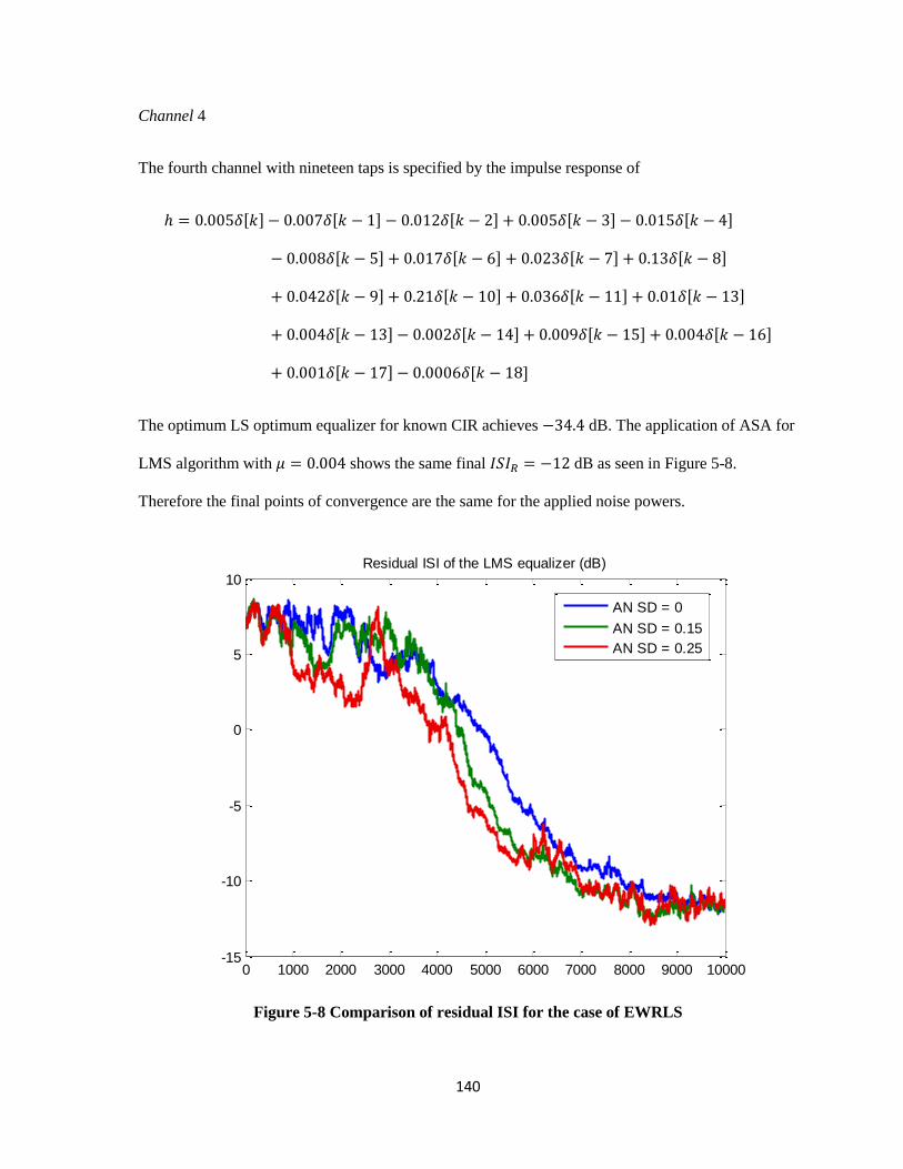
140
Channel 4
The fourth channel with nineteen taps is specified by the impulse response of
[ ] [ ] [ ] [ ] [ ]
[ ] [ ] [ ] [ ]
[ ] [ ] [ ] [ ]
[ ] [ ] [ ] [ ]
[ ] [ ]
The optimum LS optimum equalizer for known CIR achieves dB. The application of ASA for
LMS algorithm with shows the same final dB as seen in Figure 5-8.
Therefore the final points of convergence are the same for the applied noise powers.
Figure 5-8 Comparison of residual ISI for the case of EWRLS
0 1000 2000 3000 4000 5000 6000 7000 8000 9000 10000-15
-10
-5
0
5
10Residual ISI of the LMS equalizer (dB)
AN SD = 0
AN SD = 0.15
AN SD = 0.25

141
Figure 5-9 gives the convolution of the equalizer final weight vectors with the channel CIR. It is seen
that the system converges to the final point with the same residual ISI, even though there is an
associated sign inversion.
Figure 5-9 Comparison of final equalizer convolution with the CIR
0 5 10 15 20 25 30 35-0.5
0
0.5
1Convolution of CIR and LMS equalizer with annealing nouise std dev 0
0 5 10 15 20 25 30 35-1
-0.5
0
0.5Convolution of CIR and LMS equalizer with annealing nouise std dev 0.1
0 5 10 15 20 25 30 35-1
-0.5
0
0.5Convolution of CIR and LMS equalizer with annealing nouise std dev 0.25

142
For the same channel the ASA technique is applied to the EWRLS algorithm with . The
results show a variable residual ISI as seen in Figure 5-10. Therefore there are different final
converged points based on the different annealing noise power.
Figure 5-10 Comparison of residual ISI for the case of EWRLS
Figure 5-11 confirms the varied final converged points offering the convolution of the equalizer final
weight vectors with the channel CIR. It seems that some local minima have been reached and ASA
method has the catapulting effect, at least in some cases that were examined.
0 1000 2000 3000 4000 5000 6000 7000 8000 9000 10000-15
-10
-5
0
5
10
Residual ISI of the EWRLS equalizer (dB)
AN SD = 0
AN SD = 0.10
AN SD = 0.15
AN SD = 0.20
AN SD = 0.25

143
Figure 5-11 Comparison of final equalizer convolution with the CIR
0 5 10 15 20 25 30 35-1
-0.5
0
0.5Convolution of CIR and EWRLS equalizer with annealing nouise std dev 0
0 5 10 15 20 25 30 35-1
-0.5
0
0.5Convolution of CIR and EWRLS equalizer with annealing nouise std dev 0.15
0 5 10 15 20 25 30 35-0.5
0
0.5
1Convolution of CIR and EWRLS equalizer with annealing nouise std dev 0.2
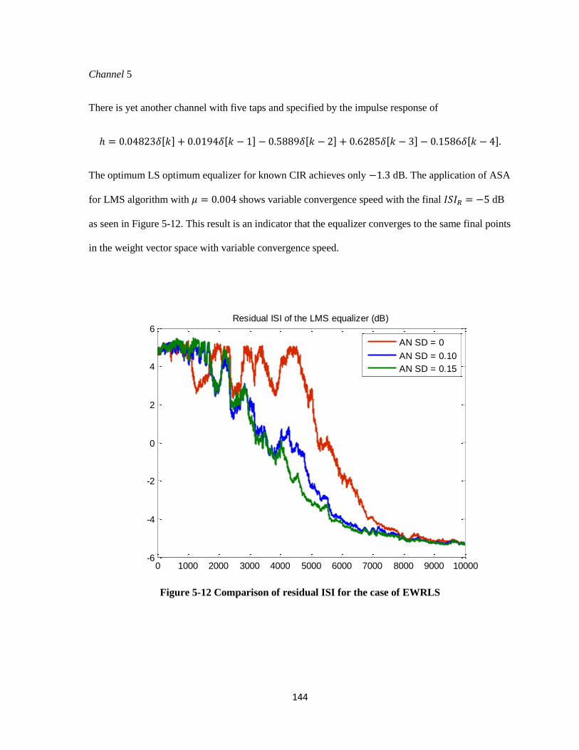
144
Channel 5
There is yet another channel with five taps and specified by the impulse response of
[ ] [ ] [ ] [ ] [ ]
The optimum LS optimum equalizer for known CIR achieves only dB. The application of ASA
for LMS algorithm with shows variable convergence speed with the final dB
as seen in Figure 5-12. This result is an indicator that the equalizer converges to the same final points
in the weight vector space with variable convergence speed.
Figure 5-12 Comparison of residual ISI for the case of EWRLS
0 1000 2000 3000 4000 5000 6000 7000 8000 9000 10000-6
-4
-2
0
2
4
6Residual ISI of the LMS equalizer (dB)
AN SD = 0
AN SD = 0.10
AN SD = 0.15
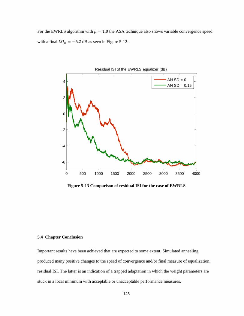
145
For the EWRLS algorithm with the ASA technique also shows variable convergence speed
with a final dB as seen in Figure 5-12.
Figure 5-13 Comparison of residual ISI for the case of EWRLS
5.4 Chapter Conclusion
Important results have been achieved that are expected to some extent. Simulated annealing
produced many positive changes to the speed of convergence and/or final measure of equalization,
residual ISI. The latter is an indication of a trapped adaptation in which the weight parameters are
stuck in a local minimum with acceptable or unacceptable performance measures.
0 500 1000 1500 2000 2500 3000 3500 4000
-6
-4
-2
0
2
4
Residual ISI of the EWRLS equalizer (dB)
AN SD = 0
AN SD = 0.15

146
Applying the ASA techniques generate results demonstrating the improvement in the convergence
speed and the final ISI. However, the final residual ISI is changed only if convergence is made to
another location of the available local minima. In other words, adding the annealing noise in any of
the different channel models will not change the performance in terms of final ISI as long as the
equalizer converges to the same point.
Another interesting observation was made about the number of local stationary points in each
algorithm. It has been seen that QS-2 algorithm shows the least number of change in the final
stationary points. The LMS algorithm comes second, and the EWRLS is first with the highest
number of change in final adapted point.
Changing the system model of Figure 5-1 to 5-2 is not associated with significant change in the
equalizers performance and behavior.

147
5.5 References
[48] Benvenuto, N., Marchesi, M., “Digital Filter Design by Simulated Annealing”, IEEE
Transactions on Circuits and Systems, Vol. 36, No. 3, March 1989.
[49] Bohm, M., et al., “On the Use of Simulated Annealing to Automatically Assign Decorrelated
Components in Second-Order Blind Source Separation”, IEEE Transactions on Biomedical
Engineering, Vol. 53, No. 5, May 2006.
[50] Courat, J.P., Raynaud, G., Wad, I., Siarry, P., “Electronic Component Model Minimization
Based on Log Simulated Annealing”, IEEE Transactions on Circuits and Systems, Vol. 41,
No. 12, December 1994.
[51] Gelfand, S.B., Mitter, S.K., “Simulated Annealing Type Algorithms for Multivariate
Optimization,” Algorithmica, pp 419-436, No. 6, 1991.
[52] Gelfand, S.B., Mitter, S.K., “Analysis of Simulated Annealing for Optimization,” Proc. 24th
Conference on Decision and Control, December 1985, pp779-786.
[53] Kirkpatrick, S, Gelatt Jr., C.D., Vecchi, M.P., “Optimization by Simulated Annealing,” IBM
Research Report RC 9355, 1982.
[54] Kirkpatrick, S, Gelatt Jr., C.D., Vecchi, M.P., “Optimization by Simulated Annealing,”
Science, Volume 220, No. 4598, May 1983.
[55] Kumar, R., “Convergence of Decision-Directed Adaptive Equalizer,” Technical Report,
Lefschetz Center for Dynamical Systems, Brown University, Providence RI, September 1981.
[56] Kumar, R., “Convergence of a Decision-Directed Adaptive Equalizer,” The 22nd
IEEE
Conference on Decision and Control, Dec. 1983.
[57] Mazo, J.C., “Analysis of Decision-Directed Equalizer Convergence,” Bell System Technical
Journal, Vol. 59, No. 10, pp 1857-1876, December 1980.
148
[58] Qin, Z., Cai, K., Zou, X., “A Reduced-Complexity Iterative Receiver Based on Simulated
Annealing for Coded partial-Response Channels”, IEEE Transactions on Magnetics, Vol. 43,
No. 6, June 2007.
[59] Rutenbar, R.A., “Simulated Annealing Algorithm: An Overview”, IEEE Circuits and Devices
magazine, Vol. 5, Issue 1, January 1989.
[60] Van Laarhoven, P.J.M., Arrts, E.H.L., “Simulated Annealing: Theory and Applications’”, D.
Reidel Publishing Company, Holland, 1987.
[61] White, L.B., Perreau, S., Duhamel, P., “Reduced Computation Blind Equalization for FIR
channel input Markov Models,” IEEE International Conference on Communications,
“Gateway to Globalization,” Seattle, 1995.
[62] Widrow, B, Walach, E., “Adaptive Inverse Control: A Signal Processing Approach,” Wiley-
IEEE Press, Nov. 2007.
149
Appendix A
Auto-covariance matrix of a random process {( )( ) } wof the random
vector with zero mean reduces to the autocorrelation matrix {( )( ) } with the following
properties. We are to show that the addition of white noise to the process output can possibly
improves the eigenvalue spread in a worst case analysis method. With the fair assumption of
stationary process the autocorrelation matrix is symmetric and also Toeplitz. Furthermore, the main
diagonal elements are all positive that can be normalized to unity. Symmetry in addition to semi-
definite properties of the autocorrelation matrix leads to real and positive eigenvalues (see Papoulis
[2]).
Let us denote the elements in a complex and square matrix order by { } , and
let denote the circles with center and radius ∑ | |
that is
{ | | | } ( )
The Greschgorin theorem states that any eigenvalue of the matrix belongs to one of the circles
(see Atkinson [1]). Since the eigenvalues of autocorrelation matrix of a stationary process are real
and positive, the Greschgorin discs geography should look like the ones in Figure A-1. Notice that
the disc centers are all equal to diagonal value . In worst case, the eigenvalue spread is
with
and as shown in Figure A-1.
Addition of white noise to the output of the process will only affect the diagonal elements to
new value . The new autocorrelation matrix has the discs geography shown in Figure A-2. In
Figure A-2 one can see the discs are all moved in the positive direction of real axis by .
Consequently the new eigenvalue spread in the worst case is
.
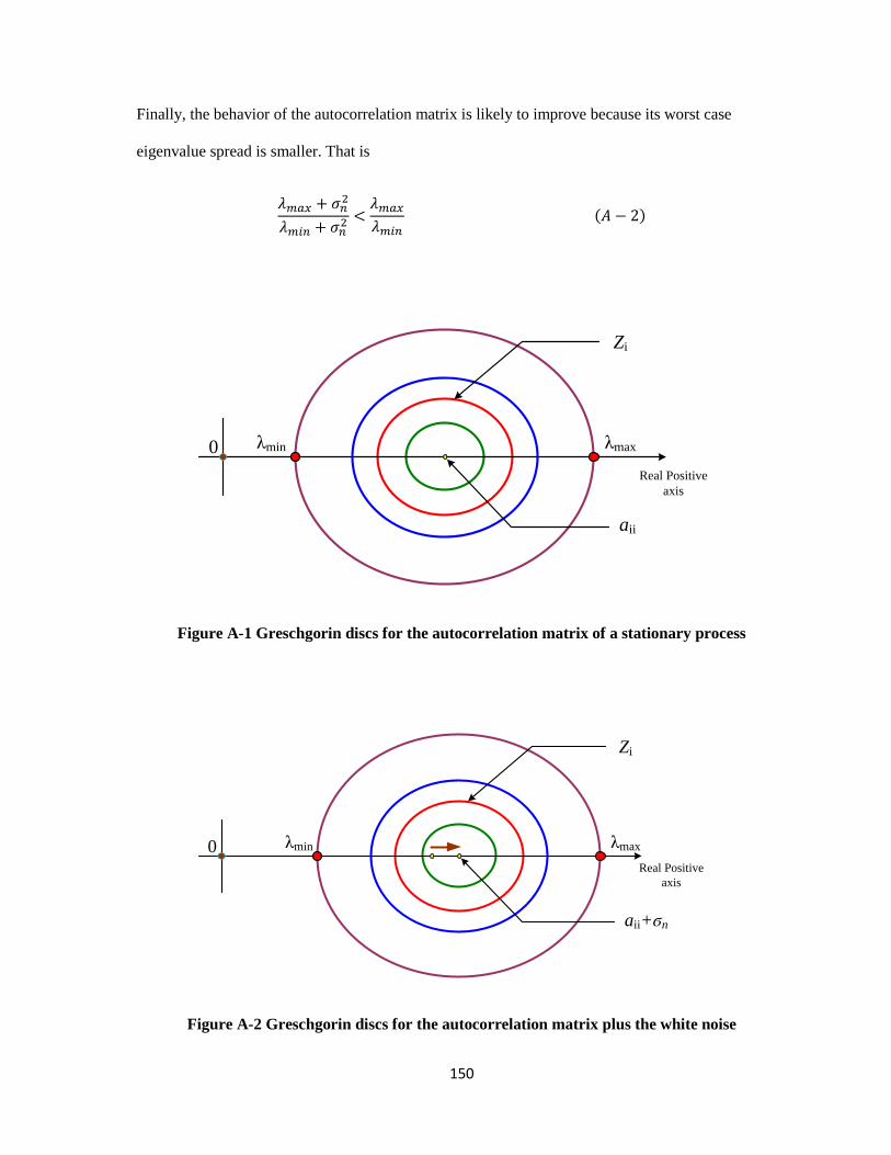
150
Finally, the behavior of the autocorrelation matrix is likely to improve because its worst case
eigenvalue spread is smaller. That is
( )
λmaxλmin
Zi
aii
0
Real Positive
axis
Figure A-1 Greschgorin discs for the autocorrelation matrix of a stationary process
λmaxλmin
Zi
aii+ϭn
0Real Positive
axis
Figure A-2 Greschgorin discs for the autocorrelation matrix plus the white noise

151
A.1 References
[1] Atkinson, K.E., “An Introduction to Numerical Analysis,” 2nd
Edition, John Wiley & Sons,
1989.
[2] Papoulis, A., Pillai, S.U., “Probabilty, Random Variables and Stochastic Processes,” 4th
Edition, McGraw-Hill Higher Education, 2002.
152
Chapter 6: Concluding Remarks and the Future Research
The main problem that is being addressed in this thesis is related the most important issues
associated with the wireless communication channels, namely Inter-Symbol Interference (ISI) caused
by multipath nature and the communicators mobility. A complete introduction to the modeling and
characteristics of this kind of channels are given in Chapter 1. It was also explained in Chapter 2 that
ISI is causing data errors and hence the main obstacle in the way of reliable and fast wireless digital
communications. The common methods to eliminate or sufficiently mitigate the effect of distortion
caused by ISI are collectively known as channel equalization.
The approach in this thesis is based not only on one methodology but several algorithms and
configurations that are offered and examined to tackle the ISI problem. There are two main
categories of channel equalization, supervised and blind modes. We have studied the application of a
new specially modified neural network requiring very short training period for the proper channel
equalization in Chapter 4. The demonstrated success in given examples motivated some convergence
analysis.
For blind modes two distinctive methodologies are presented and studied. Chapter 3 covers the
concept of multiple “cooperative” algorithms for the cases of two and three cooperative algorithms.
Several computationally effective algorithms are necessary to implement a diversified-algorithm
system. The “select absolutely larger equalized signal” versus “majority vote” methods have been
used in 2- and 3-algoirithm systems respectively, many of the demonstrated results are encouraging
for further research.
Chapter 5 involves the application of general idea of simulated annealing to the target problem of
this thesis in an adaptive. A limited strategy of constant annealing noise is experimented for testing
the same various simple algorithms as in Multiple Algorithms systems. Convergence to local
stationary points of the cost function in parameter space is clearly demonstrated and justifies the use

153
of additional noise. The capability of the adding the random noise to release the algorithm from the
local traps is established in several cases.
Each of the methods proposed and investigated invites future research and scholarly work.
1. The new supervised equalizer system based on the new neural network configuration can be
augmented by the addition of at least one hidden layer. Additional layer seeks more
computations for both the forward and the backward propagations however it is possible to
obtain significant capability in particular for the cases of nonlinear channel models. More
general convergence analysis for all layers can be attempted in the perspective regardless of
how challenging this can be.
2. Adaptive simulated Annealing method has been studied in the limiting cases such as
constant random noise power and the lack of a plan to adjust the noise power during the
adaptation. Some practical measures that can represent the unknown channel parameters
must be proposed for the noise power management. Besides, it is intuitively assumed that
there should be modified or augmented algorithms to achieve robust and mighty ASA
process with minimal constraints.
3. The algorithms with diversified adaptive techniques have been studied with limited number
and limited variety of cooperating techniques. Although the methodology for the cooperation
of algorithms can be seen to be final, there are capacities of improvements that require
scholarly attentions.