Wireless and Mobile Communications - SJTUwang-xb/wireless_new/coursePages/course... · Existing...

Wireless and Mobile Communications

Outline

• Overview

• MAC

• Routing

• Wireless in real world

• Leverage broadcasting nature

• Wireless security

2

From Wired to Wireless

The Difference: # 1

The Difference #2

Unicast vs. Broadcast

Why?

• Interference

• Your signal is noise to others

• Broadcast nature

signal - to - noise - ratio

Existing Wireless Networks

• Wireless Metropolitan Area Network (WMAN)

• Cellular/Wireless Wide Area Network (WWAN) (GSM, WCDMA, EV-DO)

• Wireless Local Area Network (WLAN)

• Wireless Personal Area Network

(WPAN)

• Ad hoc networks

• Sensor networks

• Emerging networks (variations of ad

hoc networks

• Info-stations

• Vehicular networks

• Cognitive Radio Networks

• IEEE 802.22

Data Rate

Transmission Range

Power Dissipation

Network Architectures

Cellular Networks (hierarchical systems) QoS + mobility $$$, lack of innovations

WLAN / Mesh networks Simple, cheap Poor management

Ad hoc networks no infrastructure cost no guarantee

Sensor networks Energy limited, low processing power

Challenges in Cellular Networks

• Explosion of mobile phones, 1.5billion users (2004)

• Scalability issues (particularly at radio network controller)

• Better architecture design

• Lack of bandwidth (we need mobile TV)

• Give us more spectrum

IEEE 802.11 - Architecture of an Infrastructure Network • Station (STA)

• Terminal with access mechanisms to the wireless medium and radio contact to the access point

• Basic Service Set (BSS) • Group of stations using the same

radio frequency

• Access Point • Station integrated into the wireless

LAN and the distribution system

• Portal • bridge to other (wired) networks

• Distribution System • Interconnection network to form

one logical network

Challenges in WiFi

• Again, explosion of users, devices…

• Interference, interference, interference

• Heavy interference /contention when accessing the AP, no QoS support

• Inter-AP interference

• Interference from other devices (microwave, cordless phones) in the same frequency band

• Mobility support

• Seamless roaming when users move between APs

• Normally low speed (3-10mph)

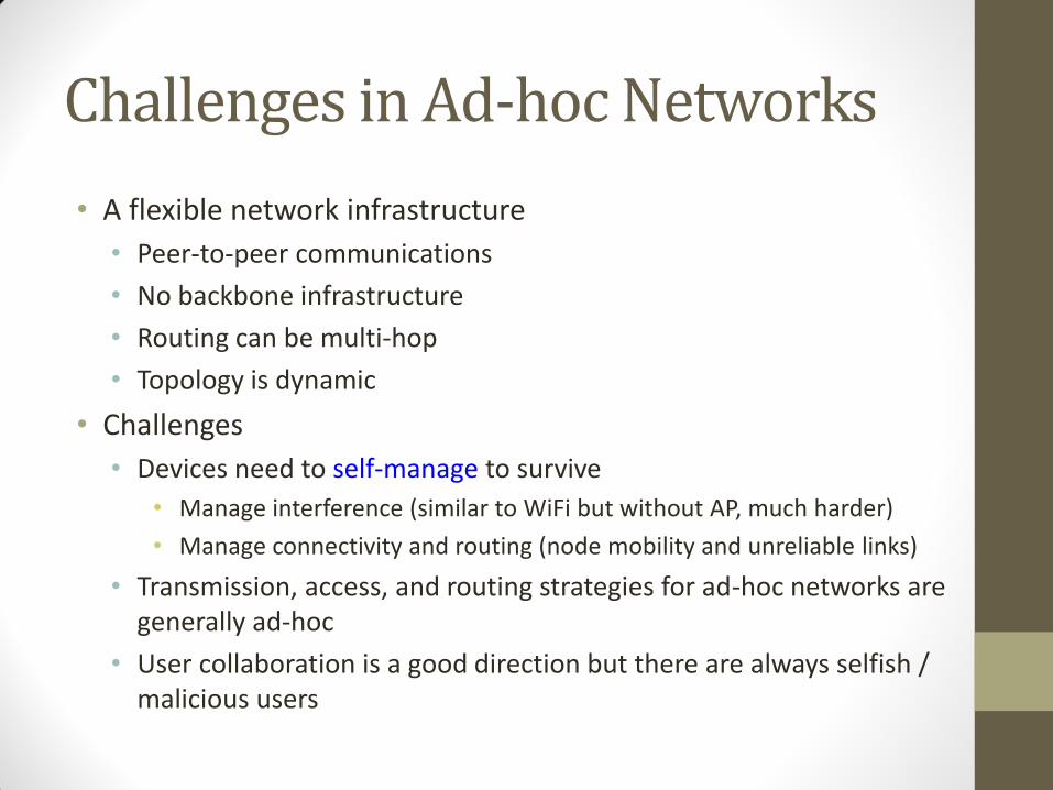
Challenges in Ad-hoc Networks

• A flexible network infrastructure

• Peer-to-peer communications

• No backbone infrastructure

• Routing can be multi-hop

• Topology is dynamic

• Challenges

• Devices need to self-manage to survive

• Manage interference (similar to WiFi but without AP, much harder)

• Manage connectivity and routing (node mobility and unreliable links)

• Transmission, access, and routing strategies for ad-hoc networks are generally ad-hoc

• User collaboration is a good direction but there are always selfish / malicious users

How does Wireless affect Networking?

• Wireless access is different from Ethernet access

• Wireless routing is different from IP routing

• Wireless security is different from wired security

Wireless Access vs. Ethernet Access

• Ethernet: fixed connection, always on, stable, fixed rate

• Wireless: unreliable connection, competition based, fading/unreliable, dynamic rate, limited bandwidth

• Critical: how to coordinate among devices to avoid interference

• Cellular: centralized, base station tells each device when and how to send/receive data

• WLAN + Ad hoc: distributed, CSMA, compete and backoff

• Mobility

• neighbor discovery + topology control

• Rate adaptations

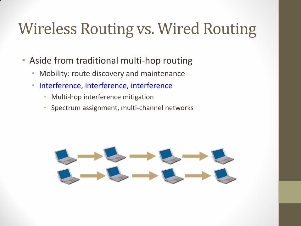
Wireless Routing vs. Wired Routing

• Aside from traditional multi-hop routing • Mobility: route discovery and maintenance

• Interference, interference, interference

• Multi-hop interference mitigation

• Spectrum assignment, multi-channel networks

So far

• Understand why wireless data rate is lower than wired…

• Understand different types of wireless networks:

• WPAN, WLAN, WWAN, WMAN and their challenges

• Understand the difference between infrastructure and ad hoc networks

• Understand the challenges in MAC, networking and security areas…

Outline

• Overview

• MAC

• Routing




23

Why Control Medium Access

• Wireless channel is a shared medium

• When conflict, interference disrupts communications

• Medium access control (MAC)

• Avoid interference

• Provide fairness

• Utilize channel variations to improve throughput

• Independent link variations

MAC Categories

Random Access

• Random Access vs. Controlled Access

• No fixed schedule, no special node to coordinate

• Distributed algorithm to determine how users share channel, when each user should transmit

• Challenges: two or more users can access the same channel simultaneously Collisions

• Protocol components:

• How to detect and avoid collisions

• How to recover from collisions

Examples

• Slotted ALOHA

• Pure ALOHA

• CSMA, CSMA/CA, CSMA/CD

The Trivial Solution

• Transmit and pray

• Plenty of collisions --> poor throughput at high load

A C B

collision

The Simple Fix

• Transmit and pray

• Plenty of collisions --> poor throughput at high load

• Listen before you talk

• Carrier sense multiple access (CSMA)

• Defer transmission when signal on channel

A C B

Don’t

transmit

Can collisions still occur?

CSMA Collisions

Collisions can still occur: Propagation delay non-zero between transmitters

When collision: Entire packet transmission time wasted

spatial layout of nodes

Note: Role of distance & propagation delay in determining collision probability

CSMA/CD (Collision Detection)

• Keep listening to channel • While transmitting

• If (Transmitted_Signal !=

Sensed_Signal) Sender knows it’s a Collision

ABORT

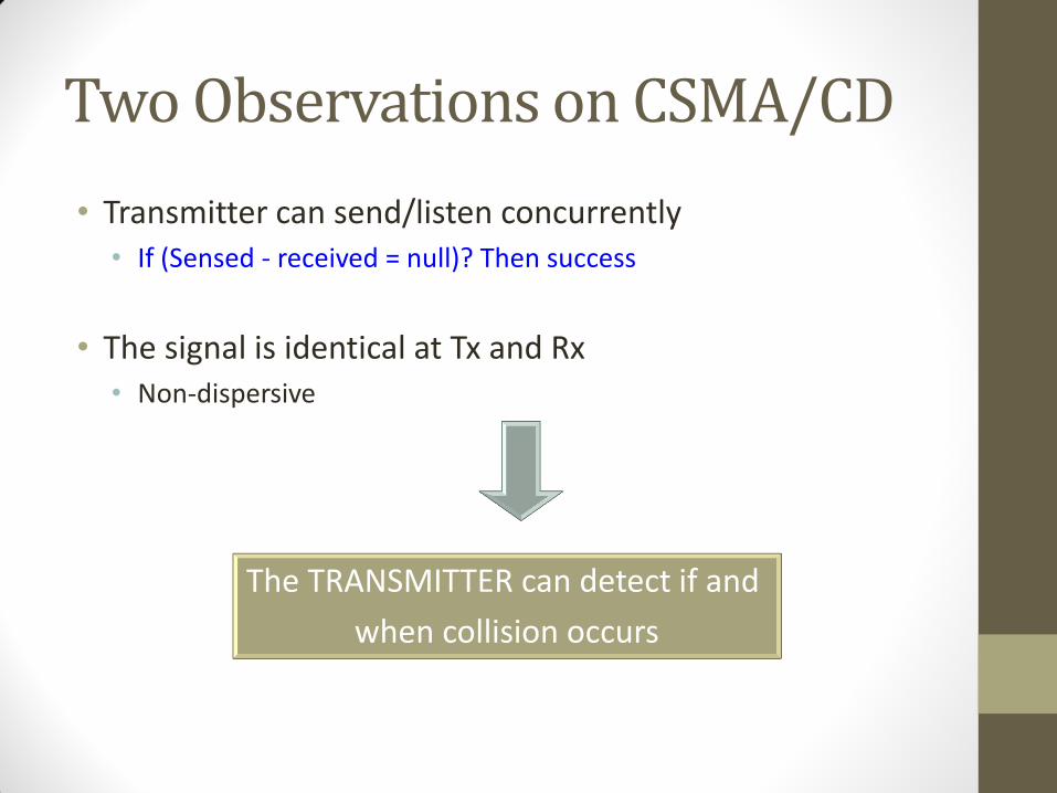
Two Observations on CSMA/CD

• Transmitter can send/listen concurrently • If (Sensed - received = null)? Then success

• The signal is identical at Tx and Rx • Non-dispersive

The TRANSMITTER can detect if and

when collision occurs

Unfortunately …

Both observations do not hold for wireless!!!

Because …

Wireless Medium Access Control

A B

C D

Distance

Signal power

SINR threhold

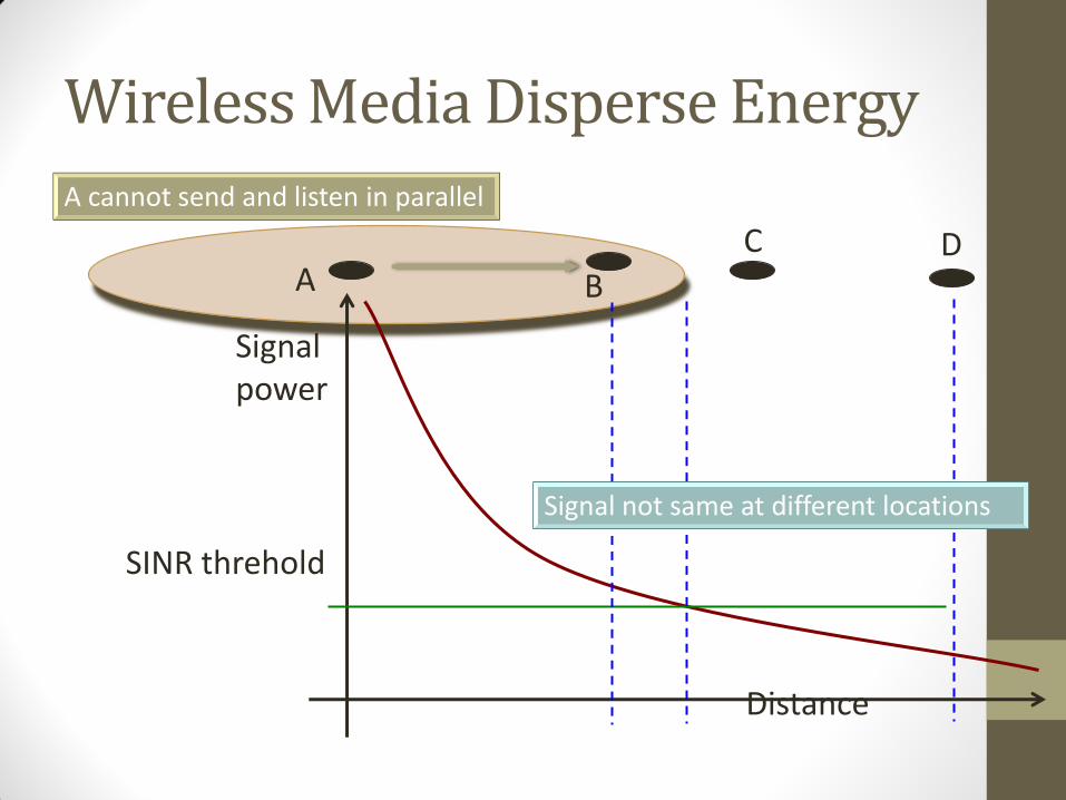
Wireless Media Disperse Energy

A cannot send and listen in parallel

Signal not same at different locations

A B

C D

Distance

Signal power

SINR threhold

• Signal reception based on SINR

• Transmitter can only hear itself

• Cannot determine signal quality at receiver

Collision Detection Difficult

A C D

B

Calculating SINR

A B

C

CB

C

transmitC

B

AB

A

A

B

d

PI

d

PSoI

NNoiseIceInterferen

SoIterestSignalOfInSINR

transmit

)()(

)(

CB

C

transmit

AB

A

A

B

d

PN

d

P

SINR

transmit

D

A B

C D

Distance

Signal power

SINR threhold

Red signal >> Blue signal

X

Red < Blue = collision

Important: C has not heard A, but can interfere at receiver B

C is the hidden terminal to A

A B

C D

Distance

Signal power

SINR threhold

X

Important: X has heard A, but should not defer transmission to Y

X is the exposed terminal to A Y

A B

C D

Distance

Signal power

SINR threhold

X

Exposed Terminal Problem (ETP)

• Don’t know whether two transmissions will conflict or not

• C wants to transmit to D but hears B; C defers transmission to D although it won’t disturb the transmission from B to A

Critical fact #1: Interference is receiver driven while CSMA is sender driven

Hidden Terminal Problem (HTP)

• Reason: limited transmit/sensing capabilities

• B can communicate with A and C

• A and C can not hear each other

• If A transmits to B & C transmits to B, collision occurs at B

6-43

CSMA/CA-Avoiding Collisions

Idea: allow sender to “reserve” channel rather than random access of data frames: avoid collisions of long data frames

• Sender first transmits small request-to-send (RTS) packets to BS using CSMA

• BS broadcasts clear-to-send CTS in response to RTS

• RTS heard by all nodes

• Sender transmits data frame

• Other stations defer transmissions

avoid data frame collisions completely using small reservation packets!

Problems with Single Channel

• Collisions happen to RTS and CTS too

• Bandwidth is limited

• Are there alternatives to avoid interference??

• Ways to avoid interference

• Time

• Space

• Frequency/channel

Multiple Channel Motivation

How to coordinate among users which channel to use?

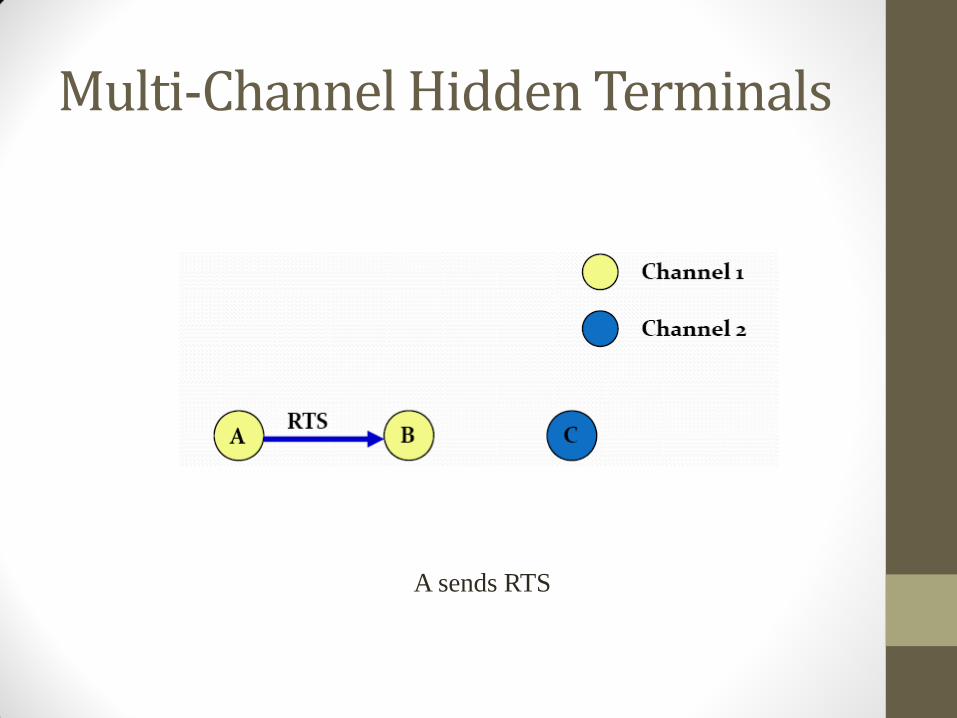
Multi‐Channel Hidden Terminals

A sends RTS


B sends CTS C does not hear CTS because C is listening on channel 2


C switches to channel 1 and transmits RTS Collision occurs at B

Outline

• Overview

• MAC

• Routing




61

Assumptions of Wireless Routing

• Inherent mobility

• Nodes are not static

• Transmission properties

• Classically assumed as unit-disc model

• All or nothing range R

• Symmetric reception

Scenarios

GOAL

• Minimize control overhead

• Minimize processing overhead

• Multi-hop path routing capability

• Dynamic topology maintenance

• No routing loops

• Self-starting

Brief Review of Internet Routing

• Intra-AS routing

• Link-state

• Distance vector

• Distance vector

• Neighbors periodically exchange routing information with neighbors

• <destination IP addr, hop count>

• Nodes iteratively learn network routing info and compute routes to all destinations

• Suffer from problems like counting-to-infinity

Review Cont.

• Link State

• Nodes flood neighbor routing information to all nodes in network

• <neighbor IP Addr, cost>

• Once each node knows all links in network, can individually compute routing paths

• Use Dijkstra for example

• Minimize routing “cost”

• Supports metrics other than hop count, but is more complex

Review Cont.

• Examples of routing protocols

• Distance vector: RIP

• Link state: OSPF

• What do these have in common?

• Both maintain routes to all nodes in network

Approaches to Wireless Routing

• Proactive Routing

• Based on traditional distance-vector and link-state protocols

• Nodes proactively maintains route to each other

• Periodic and/or event triggered routing update exchange

• Higher overhead in most scenarios

• Longer route convergence time

• Examples: DSDV, TBRPF, OLSR

Approaches Cont.

• Reactive (on-demand) Routing

• Source build routes on-demand by “flooding”

• Maintain only active routes

• Route discovery cycle

• Typically, less control overhead, better scaling properties

• Drawback??

• Route acquisition latency

• Example: AODV, DSR

WIRELESS ROUTING PROTOCOLS (1): REACTIVE PROTOCOLS

Dynamic Source Routing (DSR) [Johnson96]

• When node S wants to send a packet to node D, but does not know a route to D, node S initiates a route discovery

• Source node S floods Route Request (RREQ)

• Each node appends own identifier when forwarding RREQ

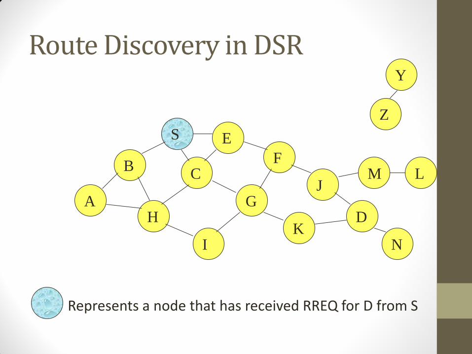
Route Discovery in DSR

B

A

S E

F

H

J

D

C

G

I K

Z

Y

Represents a node that has received RREQ for D from S

M

N

L


B

A

S E

F

H

J

D

C

G

I K

Represents transmission of RREQ

Z

Y Broadcast transmission

M

N

L

[S]

[X,Y] Represents list of identifiers appended to RREQ


B

A

S E

F

H

J

D

C

G

I K

• Node H receives packet RREQ from two neighbors: potential for collision

Z

Y

M

N

L

[S,E]

[S,C]


B

A

S E

F

H

J

D

C

G

I K

• Node C receives RREQ from G and H, but does not forward it again, because node C has already forwarded RREQ once

Z

Y

M

N

L

[S,C,G]

[S,E,F]


B

A

S E

F

H

J

D

C

G

I K

Z

Y

M

• Nodes J and K both broadcast RREQ to node D • Since nodes J and K are hidden from each other, their transmissions may collide

N

L

[S,C,G,K]

[S,E,F,J]


B

A

S E

F

H

J

D

C

G

I K

Z

Y

• Node D does not forward RREQ, because node D is the intended target of the route discovery

M

N

L

[S,E,F,J,M]


• Destination D on receiving the first RREQ, sends a Route Reply (RREP)

• RREP is sent on a route obtained by reversing the route appended to received RREQ

• RREP includes the route from S to D on which RREQ was received by node D

Route Reply in DSR

B

A

S E

F

H

J

D

C

G

I K

Z

Y

M

N

L

RREP [S,E,F,J,D]

Represents RREP control message

Route Reply in DSR

• Route Reply can be sent by reversing the route in Route Request (RREQ) only if links are guaranteed to be bi-directional • To ensure this, RREQ should be forwarded only if it received on a link

that is known to be bi-directional

• If unidirectional (asymmetric) links are allowed, then RREP may need a route discovery for S from node D • Unless node D already knows a route to node S

• If a route discovery is initiated by D for a route to S, then the Route Reply is piggybacked on the Route Request from D.

• If IEEE 802.11 MAC is used to send data, then links have to be bi-directional (since Ack is used)

Dynamic Source Routing (DSR)

• Node S on receiving RREP, caches the route included in the RREP

• When node S sends a data packet to D, the entire route is included in the packet header

• hence the name source routing

• Intermediate nodes use the source route included in a packet to determine to whom a packet should be forwarded

Data Delivery in DSR

B

A

S E

F

H

J

D

C

G

I K

Z

Y

M

N

L

DATA [S,E,F,J,D]

Packet header size grows with route length

When to Perform a Route Discovery

• When node S wants to send data to node D, but does not know a valid route node D

DSR Optimization: Route Caching

• Each node caches a new route it learns by any means

• When node S finds route [S,E,F,J,D] to node D, node S also learns route [S,E,F] to node F

• When node K receives Route Request [S,C,G] destined for node, node K learns route [K,G,C,S] to node S

• When node F forwards Route Reply RREP [S,E,F,J,D], node F learns route [F,J,D] to node D

• When node E forwards Data [S,E,F,J,D] it learns route [E,F,J,D] to node D

• A node may also learn a route when it overhears Data packets

Use of Route Caching

• When node S learns that a route to node D is broken, it uses another route from its local cache, if such a route to D exists in its cache. Otherwise, node S initiates route discovery by sending a route request

• Node X on receiving a Route Request for some node D can send a Route Reply if node X knows a route to node D

• Use of route cache

• can speed up route discovery

• can reduce propagation of route requests

Use of Route Caching

B

A

S E

F

H

J

D

C

G

I K

[P,Q,R] Represents cached route at a node (DSR maintains the cached routes in a tree format)

M

N

L

[S,E,F,J,D] [E,F,J,D]

[C,S]

[G,C,S]

[F,J,D],[F,E,S]

[J,F,E,S]

Z

Use of Route Caching: Can Speed up Route Discovery

B

A

S E

F

H

J

D

C

G

I K

Z

M

N

L


[C,S]

[G,C,S]

[F,J,D],[F,E,S]

[J,F,E,S]

RREQ

When node Z sends a route request for node C, node K sends back a route reply [Z,K,G,C] to node Z using a locally cached route

[K,G,C,S] RREP

Use of Route Caching: Can Reduce Propagation of Route Requests

B

A

S E

F

H

J

D

C

G

I K

Z

Y

M

N

L


[C,S]

[G,C,S]

[F,J,D],[F,E,S]

[J,F,E,S]

RREQ

Assume that there is no link between D and Z. Route Reply (RREP) from node K limits flooding of RREQ. In general, the reduction may be less dramatic.

[K,G,C,S]

RREP

Route Error (RERR)

B

A

S E

F

H

J

D

C

G

I K

Z

Y

M

N

L

RERR [J-D]

J sends a route error to S along route J-F-E-S when its attempt to forward the data packet S (with route SEFJD) on J-D fails Nodes hearing RERR update their route cache to remove link J-D

Route Caching: Beware!

• Stale caches can adversely affect performance

• With passage of time and host mobility, cached routes may become invalid

• A sender host may try several stale routes (obtained from local cache, or replied from cache by other nodes), before finding a good route

• An illustration of the adverse impact on TCP will be discussed later in the tutorial [Holland99]

Dynamic Source Routing: Advantages

• Routes maintained only between nodes who need to communicate

• reduces overhead of route maintenance

• Route caching can further reduce route discovery overhead

• A single route discovery may yield many routes to the destination, due to intermediate nodes replying from local caches

Dynamic Source Routing: Disadvantages • Packet header size grows with route length due to source

routing

• Flood of route requests may potentially reach all nodes in the

network

• Care must be taken to avoid collisions between route requests

propagated by neighboring nodes

• insertion of random delays before forwarding RREQ

• Increased contention if too many route replies come back due

to nodes replying using their local cache

• Route Reply Storm problem

• Reply storm may be eased by preventing a node from sending

RREP if it hears another RREP with a shorter route

Dynamic Source Routing: Disadvantages

• An intermediate node may send Route Reply using a stale cached route, thus polluting other caches

• This problem can be eased if some mechanism to purge (potentially) invalid cached routes is incorporated.

• For some proposals for cache invalidation, see [Hu00Mobicom] • Static timeouts

• Adaptive timeouts based on link stability

Flooding of Control Packets

• How to reduce the scope of the route request flood ?

• LAR [Ko98Mobicom]

• Query localization [Castaneda99Mobicom]

• How to reduce redundant broadcasts ?

• The Broadcast Storm Problem [Ni99Mobicom]

Ad Hoc On-Demand Distance Vector Routing (AODV) [Perkins99Wmcsa] • DSR includes source routes in packet headers

• Resulting large headers can sometimes degrade performance

• particularly when data contents of a packet are small

• AODV attempts to improve on DSR by maintaining routing tables at the nodes, so that data packets do not have to contain routes

• AODV retains the desirable feature of DSR that routes are maintained only between nodes which need to communicate

AODV

• Route Requests (RREQ) are forwarded in a manner similar to DSR

• When a node re-broadcasts a Route Request, it sets up a reverse path pointing towards the source

• AODV assumes symmetric (bi-directional) links

• When the intended destination receives a Route Request, it replies by sending a Route Reply

• Route Reply travels along the reverse path set-up when Route Request is forwarded

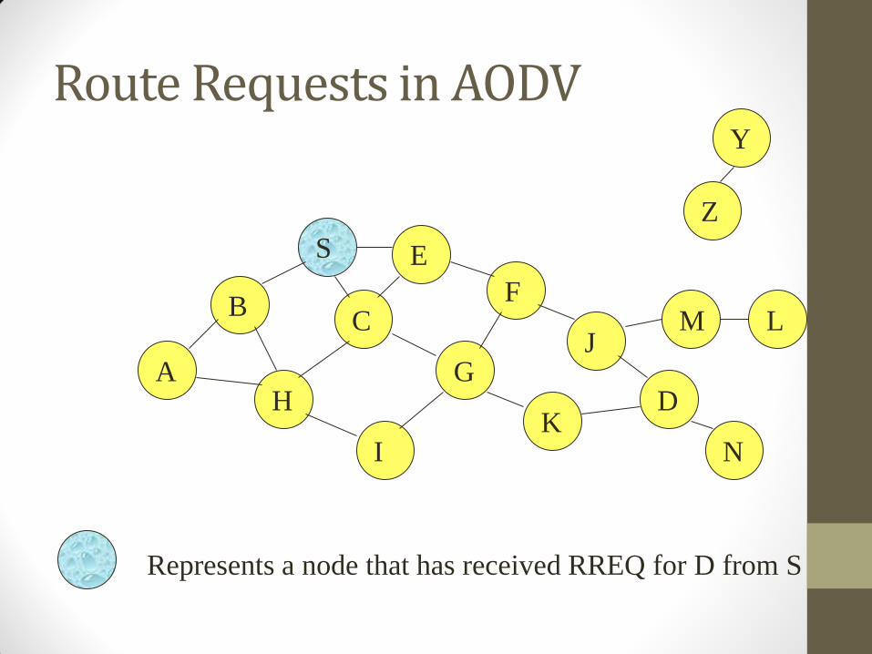
Route Requests in AODV

B

A

S E

F

H

J

D

C

G

I K

Z

Y

Represents a node that has received RREQ for D from S

M

N

L


B

A

S E

F

H

J

D

C

G

I K

Represents transmission of RREQ

Z

Y Broadcast transmission

M

N

L


B

A

S E

F

H

J

D

C

G

I K

Represents links on Reverse Path

Z

Y

M

N

L

Reverse Path Setup in AODV

B

A

S E

F

H

J

D

C

G

I K

• Node C receives RREQ from G and H, but does not forward

it again, because node C has already forwarded RREQ once

Z

Y

M

N

L


B

A

S E

F

H

J

D

C

G

I K

Z

Y

M

N

L


B

A

S E

F

H

J

D

C

G

I K

Z

Y

• Node D does not forward RREQ, because node D

is the intended target of the RREQ

M

N

L

Route Reply in AODV

B

A

S E

F

H

J

D

C

G

I K

Z

Y

Represents links on path taken by RREP

M

N

L

Route Reply in AODV • An intermediate node (not the destination) may also send a

Route Reply (RREP) provided that it knows a more recent path than the one previously known to sender S

• To determine whether the path known to an intermediate node is more recent, destination sequence numbers are used

• The likelihood that an intermediate node will send a Route Reply when using AODV not as high as DSR • A new Route Request by node S for a destination is assigned a

higher destination sequence number. An intermediate node which knows a route, but with a smaller sequence number, cannot send Route Reply

Forward Path Setup in AODV

B

A

S E

F

H

J

D

C

G

I K

Z

Y

M

N

L

Forward links are setup when RREP travels along

the reverse path

Represents a link on the forward path

Data Delivery in AODV

B

A

S E

F

H

J

D

C

G

I K

Z

Y

M

N

L

Routing table entries used to forward data packet.

Route is not included in packet header.

DATA

Timeouts

• A routing table entry maintaining a reverse path is purged after a timeout interval

• timeout should be long enough to allow RREP to come back

• A routing table entry maintaining a forward path is purged if not used for an active_route_timeout interval

• if no is data being sent using a particular routing table entry, that entry will be deleted from the routing table (even if the route may actually still be valid)

Link Failure Reporting

• A neighbor of node X is considered active for a routing table entry if the neighbor sent a packet within active_route_timeout interval which was forwarded using that entry

• When the next hop link in a routing table entry breaks, all active neighbors are informed

• Link failures are propagated by means of Route Error messages, which also update destination sequence numbers

Route Error

• When node X is unable to forward packet P (from node S to node D) on link (X,Y), it generates a RERR message

• Node X increments the destination sequence number for D cached at node X

• The incremented sequence number N is included in the RERR

• When node S receives the RERR, it initiates a new route discovery for D using destination sequence number at least as large as N

Destination Sequence Number

• Continuing from the previous slide …

• When node D receives the route request with destination sequence number N, node D will set its sequence number to N, unless it is already larger than N

Link Failure Detection

• Hello messages: Neighboring nodes periodically exchange hello message

• Absence of hello message is used as an indication of link failure

• Alternatively, failure to receive several MAC-level acknowledgement may be used as an indication of link failure

Why Sequence Numbers in AODV

• To avoid using old/broken routes

• To determine which route is newer

• To prevent formation of loops

• Assume that A does not know about failure of link C-D because RERR sent by C is lost

• Now C performs a route discovery for D. Node A receives the RREQ (say, via path C-E-A)

• Node A will reply since A knows a route to D via node B

• Results in a loop (for instance, C-E-A-B-C )

A B C D

E

Why Sequence Numbers in AODV

• Loop C-E-A-B-C

A B C D

E

WIRELESS ROUTING PROTOCOLS (2): PROACTIVE PROTOCOLS

Proactive Protocols

• Most of the schemes discussed so far are reactive

• Proactive schemes based on distance-vector and link-state mechanisms have also been proposed

Link State Routing [Huitema95]

• Each node periodically floods status of its links

• Each node re-broadcasts link state information received from its neighbor

• Each node keeps track of link state information received from other nodes

• Each node uses above information to determine next hop to each destination

Optimized Link State Routing (OLSR) [Jacquet00ietf, Jacquet99Inria] • The overhead of flooding link state information is reduced by

requiring fewer nodes to forward the information

• A broadcast from node X is only forwarded by its multipoint relays

• Multipoint relays of node X are its neighbors such that each two-hop neighbor of X is a one-hop neighbor of at least one multipoint relay of X

• Each node transmits its neighbor list in periodic beacons, so that all nodes can know their 2-hop neighbors, in order to choose the multipoint relays

Optimized Link State Routing (OLSR)

• Nodes C and E are multipoint relays of node A

A

B F

C

D

E H

G K

J

Node that has broadcast state information from A

Optimized Link State Routing (OLSR)

• Nodes C and E forward information received from A

A

B F

C

D

E H

G K

J


Optimized Link State Routing (OLSR) • Nodes E and K are multipoint relays for node H

• Node K forwards information received from H

• E has already forwarded the same information once

A

B F

C

D

E H

G K

J


OLSR

• OLSR floods information through the multipoint relays

• The flooded itself is fir links connecting nodes to respective multipoint relays

• Routes used by OLSR only include multipoint relays as intermediate nodes

Destination-Sequenced Distance-Vector (DSDV) [Perkins94Sigcomm] • Each node maintains a routing table which stores

• next hop towards each destination

• a cost metric for the path to each destination

• a destination sequence number that is created by the destination itself

• Sequence numbers used to avoid formation of loops

• Each node periodically forwards the routing table to its neighbors

• Each node increments and appends its sequence number when sending its local routing table

• This sequence number will be attached to route entries created for this node

Destination-Sequenced Distance-Vector (DSDV) • Assume that node X receives routing information from Y about

a route to node Z

• Let S(X) and S(Y) denote the destination sequence number for node Z as stored at node X, and as sent by node Y with its routing table to node X, respectively

X Y Z

Destination-Sequenced Distance-Vector (DSDV) • Node X takes the following steps:

• If S(X) > S(Y), then X ignores the routing information received from Y

• If S(X) = S(Y), and cost of going through Y is smaller than the route known to X, then X sets Y as the next hop to Z

• If S(X) < S(Y), then X sets Y as the next hop to Z, and S(X) is updated to equal S(Y)

X Y Z

WIRELESS ROUTING PROTOCOLS (1): HYBRID PROTOCOLS

Zone Routing Protocol (ZRP) [Haas98] Zone routing protocol combines

• Proactive protocol: which pro-actively updates network state and maintains route regardless of whether any data traffic exists or not

• Reactive protocol: which only determines route to a destination if there is some data to be sent to the destination

ZRP

• All nodes within hop distance at most d from a node X are said to be in the routing zone of node X

• All nodes at hop distance exactly d are said to be peripheral nodes of node X’s routing zone

ZRP

• Intra-zone routing: Pro-actively maintain state information for links within a short distance from any given node

• Routes to nodes within short distance are thus maintained proactively (using, say, link state or distance vector protocol)

• Inter-zone routing: Use a route discovery protocol for determining routes to far away nodes. Route discovery is similar to DSR with the exception that route requests are propagated via peripheral nodes.

ZRP: Example with Zone Radius = d = 2

S C A

E F

B

D

S performs route

discovery for D

Denotes route request

ZRP: Example with d = 2

S C A

E F

B

D

S performs route

discovery for D

Denotes route reply

E knows route from E to D,

so route request need not be

forwarded to D from E

ZRP: Example with d = 2

S C A

E F

B

D

S performs route

discovery for D

Denotes route taken by Data

Outline

• Overview

• MAC

• Routing




157

Wireless in the Real World

•Real world deployment patterns

•Mesh networks and deployments

Wireless Challenges • Force us to rethink many assumptions

• Need to share airwaves rather than wire

• Don’t know what hosts are involved

• Host may not be using same link technology

• Mobility

• Other characteristics of wireless

• Noisy lots of losses

• Slow

• Interaction of multiple transmitters at receiver

• Collisions, capture, interference

• Multipath interference

Overview

• IEEE 802.11

• Deployment patterns

• Reaction to interference

• Interference mitigation

• Mesh networks

• Architecture

• Measurements

Characterizing Current Deployments

• Datasets

• Place Lab: 28,000 APs

• MAC, ESSID, GPS

• Selected US cities

• www.placelab.org

• Wifimaps: 300,000 APs

• MAC, ESSID, Channel, GPS (derived)

• wifimaps.com

• Pittsburgh Wardrive: 667 APs

• MAC, ESSID, Channel, Supported Rates, GPS

AP Stats, Degrees: Placelab

Portland 8683 54

San Diego 7934 76

San

Francisco 3037 85

Boston 2551 39

#APs Max. degree

(Placelab: 28000 APs, MAC, ESSID, GPS)

1 2 1

50 m (i.e., # neighbors)

Degree Distribution: Place Lab

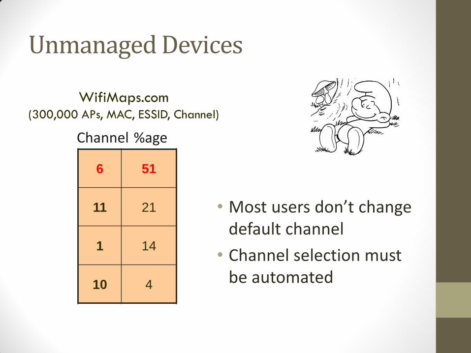
Unmanaged Devices

• Most users don’t change default channel

• Channel selection must be automated

6 51

11 21

1 14

10 4

Channel %age

WifiMaps.com (300,000 APs, MAC, ESSID, Channel)

Growing Interference in Unlicensed Bands

• Anecdotal evidence of problems, but how severe?

• Characterize how IEEE 802.11 operates under interference in practice

Other 802.11

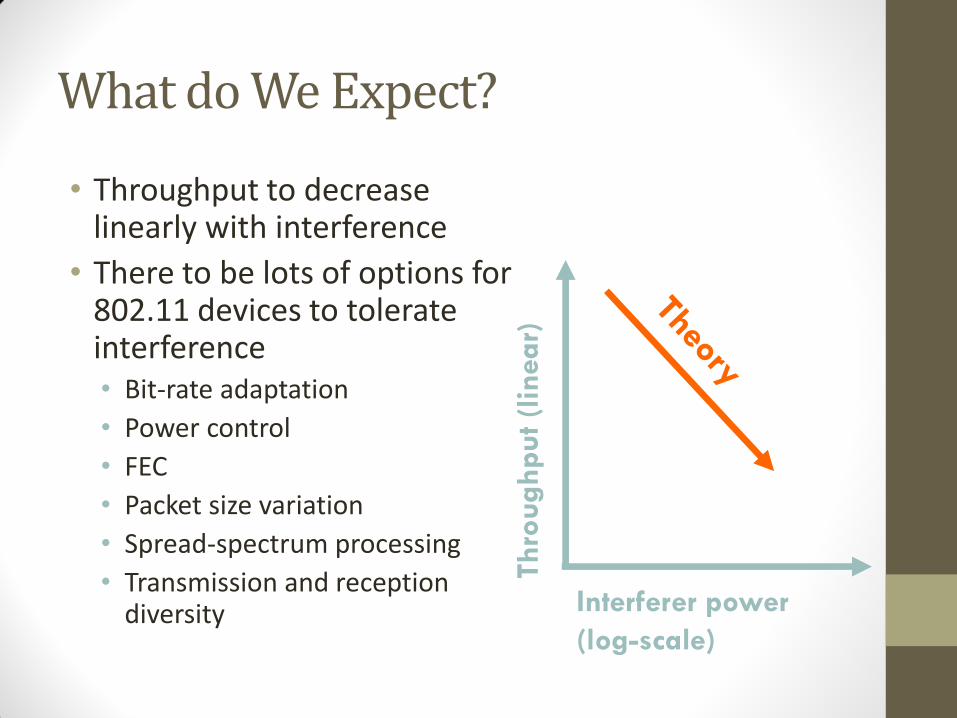
What do We Expect?

• Throughput to decrease linearly with interference

• There to be lots of options for 802.11 devices to tolerate interference • Bit-rate adaptation

• Power control

• FEC

• Packet size variation

• Spread-spectrum processing

• Transmission and reception diversity

Interferer power

(log-scale)

Thro

ughput (l

inear)

Key Questions

• How damaging can a low-power and/or narrow-band interferer be?

• How can today’s hardware tolerate interference well?

• What 802.11 options work well, and why?

What We See

• Effects of interference more severe in practice

• Caused by hardware limitations of commodity cards, which theory doesn’t model Interferer power

(log-scale)

Thro

ughput (l

inear)

Experimental Setup

802.11

Client

Access

Point

UDP flow

802.11 Interferer

802.11 Receiver Path

• Extend SINR model to capture these vulnerabilities • Interested in worst-case natural or adversarial interference

• Have developed range of “attacks” that trigger these vulnerabilities

MAC PHY

Timing Recovery

Preamble Detector/ Header CRC-16 Checker

AGC

Barker Correlator

Descrambler

ADC

6-bit samples

To RF Amplifiers

RF Signal

Receiver

Data (includes beacons)

Demodulator

PHY MAC

Analog signal

Amplifier control

SYNC SFD CRC Payload

PHY header

Timing Recovery Interference

• Interferer sends continuous SYNC pattern

• Interferes with packet acquisition (PHY reception errors)

0.1

1

10

100

1000

10000

−∞ -20 -12 -2 0 8 12 15 20

Interferer Power (dBm)

Th

rou

gh

pu

t (k

bp

s)

0

200

400

600

800

1000

1200

La

ten

cy

(mic

ros

ec

on

ds

)

Throughput

Latency

Weak interferer

Moderate

interferer

Log-scale

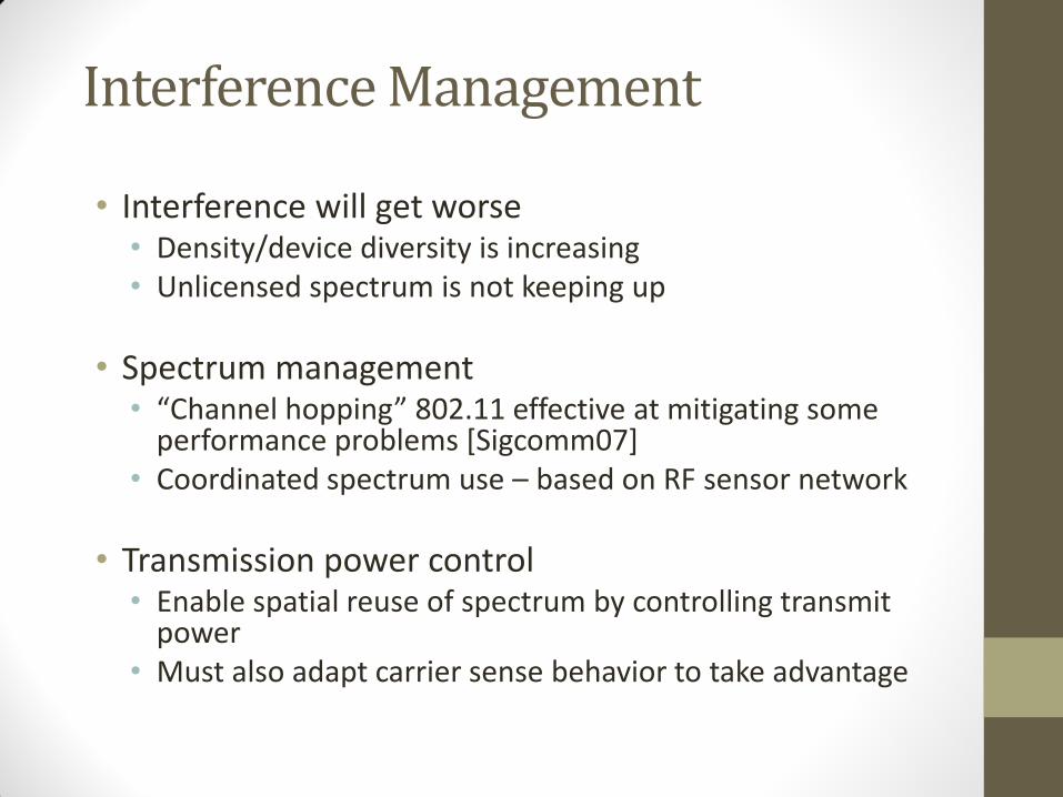
Interference Management

• Interference will get worse • Density/device diversity is increasing • Unlicensed spectrum is not keeping up

• Spectrum management • “Channel hopping” 802.11 effective at mitigating some

performance problems [Sigcomm07] • Coordinated spectrum use – based on RF sensor network

• Transmission power control • Enable spatial reuse of spectrum by controlling transmit

power • Must also adapt carrier sense behavior to take advantage

Impact of frequency separation

• Even small frequency separation (i.e., adjacent 802.11 channel) helps

0.1

1

10

100

1000

10000

−∞ -20 -12 0 8 12 15 20

Interferer Power (dBm)

Th

rou

gh

pu

t (k

bp

s) 10MHz separation

15MHz separation

Same channel

(poor performance)

5MHz separation

(good performance)

Transmission Power Control

• Choose transmit power levels to maximize physical spatial reuse

• Tune MAC to ensure nodes transmit simultaneously when possible

• Spatial reuse = network capacity / link capacity

AP1 AP2

Client1

Client2

AP1

AP2

Client1

Client2

Spatial Reuse = 1 Spatial Reuse = 2

Concurrent transmissions increase spatial reuse

Transmission Power Control in Practice

• For simple scenario easy to compute optimal transmit power • May or may not enable simultaneous

transmit

• Protocol builds on iterative pair-wise optimization

• Adjusting transmit power requires adjusting carrier sense thresholds • Echos, Alpha or eliminate carrier sense

• Altrusitic Echos – eliminates starvation in Echos

AP1

AP2

Client1

Client2

d11

d22

d12

d21

Details of Power Control

• Hard to do per-packet with many NICs • Some even might have to re-init (many ms)

• May have to balance power with rate • Reasonable goal: lowest power for max rate

• But finding ths empirically is hard! Many {power, rate} combinations, and not always easy to predict how each will perform

• Alternate goal: lowest power for max needed rate • But this interacts with other people because you use more

channel time to send the same data. Uh-oh.

• Nice example of the difficulty of local vs. global optimization

Rate Adaptation

• General idea:

• Observe channel conditions like SNR (signal-to-noise ratio), bit errors, packet errors

• Pick a transmission rate that will get best goodput • There are channel conditions when reducing the bitrate can

greatly increase throughput – e.g., if a ½ decrease in bitrate gets you from 90% loss to 10% loss.

Simple Rate Adaptation Scheme

• Watch packet error rate over window (K packets or T seconds)

• If loss rate > threshhigh (or SNR <, etc) • Reduce Tx rate

• If loss rate < threshlow

• Increase Tx rate

• Most devices support a discrete set of rates • 802.11 – 1, 2, 5.5, 11Mbps, etc.

Challenges in Rate Adaptation

• Channel conditions change over time

• Loss rates must be measured over a window

• SNR estimates from the hardware are coarse, and don’t always predict loss rate

• May be some overhead (time, transient interruptions, etc.) to changing rates

Power and Rate Selection Algorithms

• Rate Selection • Auto Rate Fallback: ARF • Estimated Rate Fallback: ERF

• Goal: Transmit at minimum necessary power to reach

receiver • Minimizes interference with other nodes • Paper: Can double or more capacity, if done right.

• Joint Power and Rate Selection

• Power Auto Rate Fallback: PARF • Power Estimated Rate Fallback: PERF • Conservative Algorithms

• Always attempt to achieve highest possible modulation rate

Power Control/Rate Control Summary

• Complex interactions…. • More power:

• Higher received signal strength • May enable faster rate (more S in S/N)

• May mean you occupy media for less time

• Interferes with more people

• Less power • Interfere with fewer people

• Less power + less rate • Fewer people but for a longer time

• Gets even harder once you consider • Carrier sense • Calibration and measurement error • Mobility

Overview

• 802.11

• Deployment patterns

• Reaction to interference

• Interference mitigation

• Mesh networks

• Architecture

• Measurements

Community Wireless Network

• Share a few wired Internet connections

• Construction of community networks

• Multi-hop network

• Nodes in chosen locations

• Directional antennas

• Require well-coordination

• Access point

• Clients directly connect

• Access points operates independently

• Do not require much coordination

Roofnet

• Goals • Operate without extensive planning or central management

• Provide wide coverage and acceptable performance

• Design decisions • Unconstrained node placement

• Omni-directional antennas

• Multi-hop routing

• Optimization of routing for throughput in a slowly changing network

Roofnet Design

• Deployment • Over an area of about four square kilometers in Cambridge,

Messachusetts • Most nodes are located in buildings

• 3~4 story apartment buildings • 8 nodes are in taller buildings

• Each Rooftnet node is hosted by a volunteer user • Hardware

• PC, omni-directional antenna, hard drive … • 802.11b card

• RTS/CTS disabled • Share the same 802.11b channel • Non-standard “pseudo-IBSS” mode

• Similar to standard 802.11b IBSS (ad hoc) • Omit beacon and BSSID (network ID)

Roofnet Node Map

1 kilometer

Roofnet

Typical Rooftop View

A Roofnet Self-Installation Kit

Computer ($340)

533 MHz PC, hard disk, CDROM

802.11b card ($155)

Engenius Prism 2.5, 200mW

Software (“free”)

Our networking software based on Click

Antenna ($65)

8dBi, 20 degree vertical

Miscellaneous ($75)

Chimney Mount, Lightning Arrestor, etc.

50 ft. Cable ($40)

Low loss (3dB/100ft)

Takes a user about 45 minutes to install on a flat roof

Total: $685

Software and Auto-Configuration

• Linux, routing software, DHCP server, web server … • Automatically solve a number of problems

• Allocating addresses • Finding a gateway between Roofnet and the Internet • Choosing a good multi-hop route to that gateway

• Addressing • Roofnet carries IP packets inside its own header format and routing

protocol • Assign addresses automatically • Only meaningful inside Roofnet, not globally routable • The address of Roofnet nodes

• Low 24 bits are the low 24 bits of the node’s Ethernet address • High 8 bits are an unused class-A IP address block

• The address of hosts • Allocate 192.168.1.x via DHCP and use NAT between the Ethernet and

Roofnet

Software and Auto-Configuration

• Gateway and Internet Access

• A small fraction of Roofnet users will share their wired Internet access links

• Nodes which can reach the Internet • Advertise itself to Roofnet as an Internet gateway

• Acts as a NAT for connection from Roofnet to the Internet

• Other nodes • Select the gateway which has the best route metric

• Roofnet currently has four Internet gateways

Evaluation

• Method

• Multi-hop TCP

• 15 second one-way bulk TCP transfer between each pair of Roofnet nodes

• Single-hop TCP

• The direct radio link between each pair of routes

• Loss matrix

• The loss rate between each pair of nodes using 1500-byte broadcasts

• Multi-hop density

• TCP throughput between a fixed set of four nodes

• Varying the number of Roofnet nodes that are participating in routing

Evaluation

• Basic Performance (Multi-hop TCP) • The routes with low hop-count have much higher

throughput • Multi-hop routes suffer from inter-hop collisions

Evaluation

• Basic Performance (Multi-hop TCP)

• TCP throughput to each node from its chosen gateway

• Round-trip latencies for 84-byte ping packets to estimate interactive delay

No problem in interactive sessions

Evaluation

• Link Quality and Distance (Single-hop TCP, Multi-hop TCP) • Most available links are between 500m and 1300m and 500 kbits/s

(most cases)

• Srcr

• Use almost all of the links faster than 2 Mbits/s and ignore majority of the links which are slower than that

• Fast short hops are the best policy

a small number of links a few hundred meters long with throughputs of two megabits/second or more, and a few longer high-throughput links

Evaluation

• Link Quality and Distance (Multi-hop TCP, Loss matrix) • Median delivery probability is 0.8

• 1/4 links have loss rates of 50% or more • 802.11 detects the losses with its ACK mechanism and resends

the packets meaning that Srcr often uses links

with loss rates of 20% or more.

Evaluation

• Architectural Alternatives • Maximize the number of additional nodes with non-zero throughput to

some gateway

• Ties are broken by average throughput

Comparison of multi-hop and single-hop

architectures, with “optimal" choice of gateways. Comparison of multi-hop and single-hop

architectures with random gateway choice.

Comparison against communication over a direct radio link to a gateway (Access-point Network)

For small numbers of gateways, multi-hop routing improves both connectivity and throughput.

Evaluation

• Inter-hop Interference (Multi-hop TCP, Single-hop TCP) • Concurrent transmissions on different hops of a route collide and

cause packet loss

The expected multi-hop throughputs are mostly higher than the measured throughputs.

Roofnet Summary

• The network’s architectures favors

• Ease of deployment

• Omni-directional antennas

• Self-configuring software

• Link-quality-aware multi-hop routing

• Evaluation of network performance

• Average throughput between nodes is 627kbits/s

• Well served by just a few gateways whose position is determined by convenience

• Multi-hop mesh increases both connectivity and throughput

Roofnet Link Level Measurements

• Analyze cause of packet loss

• Neighbor Abstraction

• Ability to hear control packets or No Interference

• Strong correlation between BER and S/N

• RoofNet pairs communicate

• At intermediate loss rates

• Temporal Variation

• Spatial Variation

neighbor abstraction is a poor approximation of reality

Lossy Links are Common

Delivery Probabilities are Uniformly Distributed

Delivery vs. SNR

• SNR not a good predictor

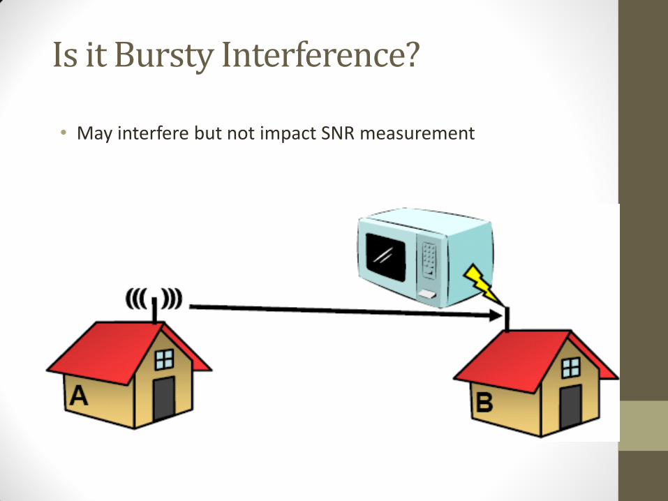
Is it Bursty Interference?

• May interfere but not impact SNR measurement

Two Different Roofnet Links

• Top is typical of bursty interference, bottom is not

• Most links are like the bottom

Is it Multipath Interference?

• Simulate with channel emulator

A Plausible Explanation

• Multi-path can produce intermediate loss rates

• Appropriate multi-path delay is possible due to long-links

Key Implications

• Lack of a link abstraction!

• Links aren’t on or off… sometimes in-between

• Protocols must take advantage of these intermediate quality links to perform well

• How unique is this to Roofnet?

• Cards designed for indoor environments used outdoors

Outline

• Overview

• MAC

• Routing




209

Taking Advantage of Broadcast

•Opportunistic forwarding (ExOR)

•Network coding (COPE)

packet

packet

packet

Initial Approach: Traditional Routing

• Identify a route, forward over links

• Abstract radio to look like a wired link

src

A B

dst

C

Radios Aren’t Wires

• Every packet is broadcast

• Reception is probabilistic

1 2 3 4 5 6 1 2 3 6 3 5 1 4 2 3 4 5 6 1 2 4 5 6 src

A B

dst

C

packet

packet packet packet packet packet

Exploiting Probabilistic Broadcast

src

A B

dst

C

packet packet packet

• Decide who forwards after reception

• Goal: only closest receiver should forward

• Challenge: agree efficiently and avoid duplicate transmissions

Why ExOR Might Increase Throughput

• Best traditional route over 50% hops: 3(1/0.5) = 6 tx

• Throughput 1/# transmissions

• ExOR exploits lucky long receptions: 4 transmissions

• Assumes probability falls off gradually with distance

src dst N1 N2 N3 N4

75% 50%

N5

25%

Why ExOR Might Increase Throughput

• Traditional routing: 1/0.25 + 1 = 5 tx

• ExOR: 1/(1 – (1 – 0.25)4) + 1 = 2.5 transmissions

• Assumes independent losses

N1

src dst

N2

N3

N4

Comparing ExOR

• Traditional Routing:

• One path followed from source to destination

• All packets sent along that path

• Co-operative Diversity:

• Broadcast of packets by all nodes

• Destination chooses the best one

• ExOR:

• Broadcast packets to all nodes

• Only one node forwards the packet

• Basic idea is delayed forwarding

ExOR Batching

• Challenge: finding the closest node to have rx’d

• Send batches of packets for efficiency

• Node closest to the dst sends first • Other nodes listen, send remaining packets in turn

• Repeat schedule until dst has whole batch

src

N3

dst

N4

tx: 23

tx: 57 -23

24

tx: 8

tx: 100

rx: 23

rx: 57

rx: 88

rx: 0

rx: 0 tx: 0

tx: 9

rx: 53

rx: 85

rx: 99

rx: 40

rx: 22

N1

N2

Reliable Summaries

• Repeat summaries in every data packet • Cumulative: what all previous nodes rx’d • This is a gossip mechanism for summaries

src

N1

N2

N3

dst

N4

tx: {1, 6, 7 ... 91, 96, 99}

tx: {2, 4, 10 ... 97, 98} batch map: {1,2,6, ... 97, 98, 99}

batch map: {1, 6, 7 ... 91, 96, 99}

contains the sender's best guess of the highest priority node to have received each packet

The remaining forwarders transmit in order, but only send packets which were not acknowledged in the batch maps of higher priority nodes.

Priority Ordering

• Goal: nodes “closest” to the destination send first • Sort by ETX metric to dst • Nodes periodically flood ETX “link state” measurements • Path ETX is weighted shortest path (Dijkstra’s algorithm)

• Source sorts, includes list in ExOR header

src

N1

N2

N3

dst

N4

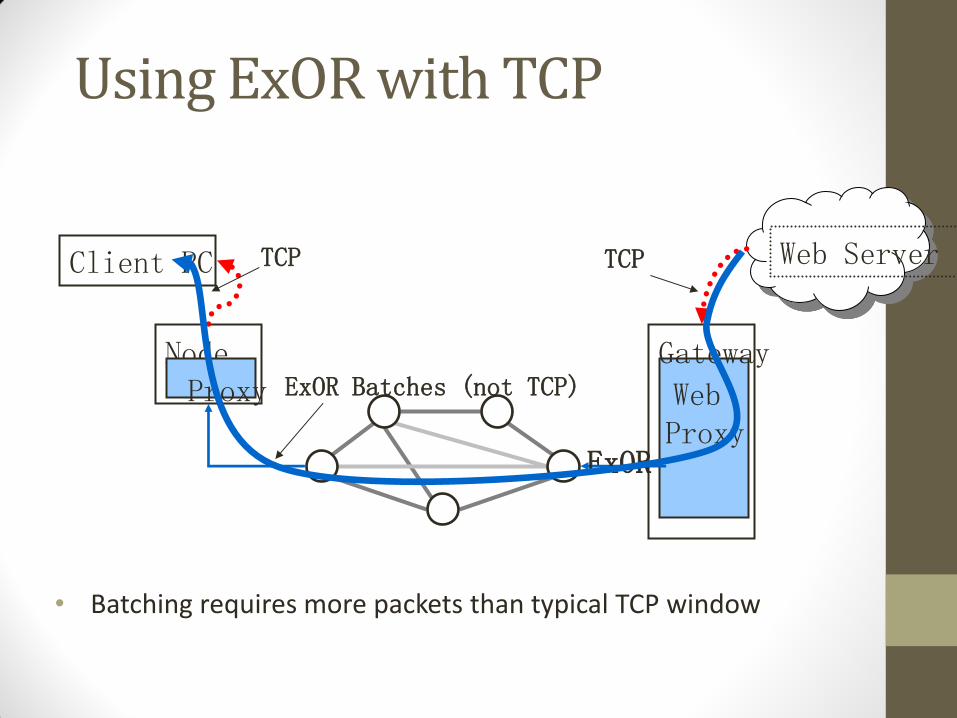
Using ExOR with TCP

Node Proxy

ExOR

Gateway

Web Proxy

Client PC Web Server TCP TCP

ExOR Batches (not TCP)

• Batching requires more packets than typical TCP window

Summary

• ExOR achieves 2x throughput improvement

• ExOR implemented on Roofnet

• Exploits radio properties, instead of hiding them

Outline

•Opportunistic forwarding (ExOR)

•Network coding (COPE)

Background

• Famous butterfly example:

• All links can send one message per unit of time • Coding increases overall throughput

Background

• Bob and Alice

Relay

Require 4 transmissions

Background

• Bob and Alice

Relay

Require 3 transmissions

XOR

XOR XOR

Coding Gain

• Coding gain = 4/3

1 1+3

3

Throughput Improvement

• UDP throughput improvement ~ a factor 2 > 4/3 coding gain

1 1+3

3

Coding Gain: more examples

Without opportunistic listening, coding [+MAC] gain=2N/(1+N) 2.

With opportunistic listening, coding gain + MAC gain ∞

3

5

1+2+3+4+5

2

4

1 Opportunistic Listening:

Every node listens to all

packets

It stores all heard

packets for a limited

time

COPE (Coding Opportunistically)

• Overhear neighbors’ transmissions

• Store these packets in a Packet Pool for a short time

• Report the packet pool info. to neighbors

• Determine what packets to code based on the info.

• Send encoded packets

• To send packet p to neighbor A, XOR p with packets already known to A. Thus, A can decode

• But how can multiple neighbors benefit from a single transmission?

Opportunistic Coding

B’s queue Next hop

P1 A

P2 C

P3 C

P4 D

Coding Is it good?

P1+P2 Bad (only C can decode)

P1+P3 Better coding (Both A and C can decode)

P1+P3+P4 Best coding (A, C, D can decode)

B

A

C

D

P4 P3 P3 P1

P4 P3 P2 P1

P4 P1

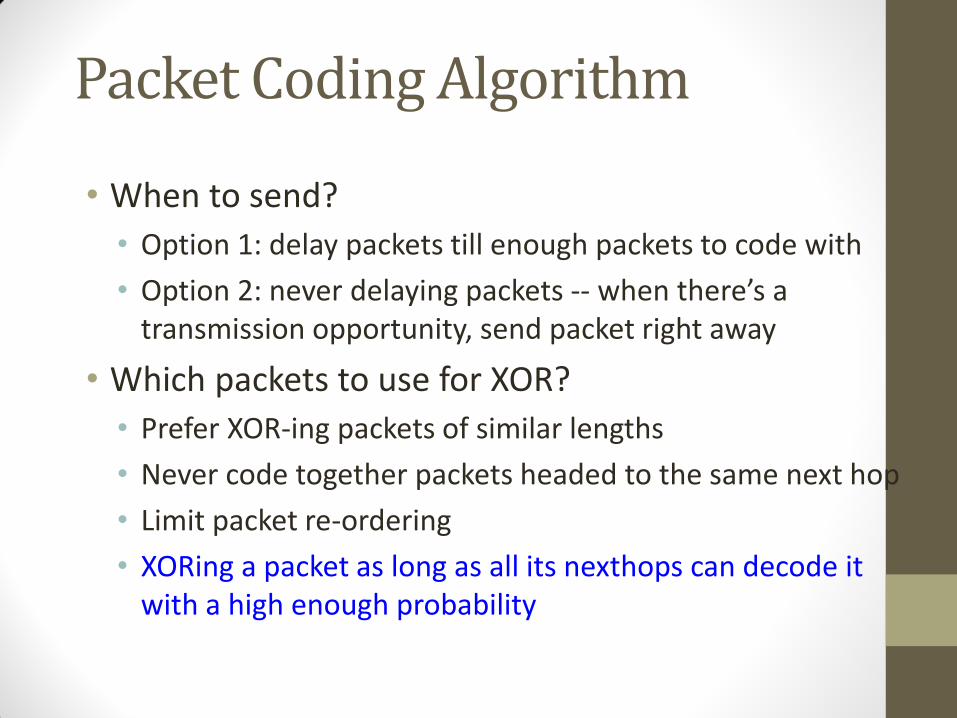
Packet Coding Algorithm

• When to send?

• Option 1: delay packets till enough packets to code with

• Option 2: never delaying packets -- when there’s a transmission opportunity, send packet right away

• Which packets to use for XOR?

• Prefer XOR-ing packets of similar lengths

• Never code together packets headed to the same next hop

• Limit packet re-ordering

• XORing a packet as long as all its nexthops can decode it with a high enough probability

Packet Decoding

• Where to decode?

• Decode at each intermediate hop

• How to decode?

• Upon receiving a packet encoded with n native packets

• find n-1 native packets from its queue

• XOR these n-1 native packets with the received packet to extract the new packet

Prevent Packet Reordering

• Packet reordering due to async acks degrade TCP performance

• Ordering agent

• Deliver in-sequence packets immediately

• Order the packets until the gap in seq. no is filled or timer expires

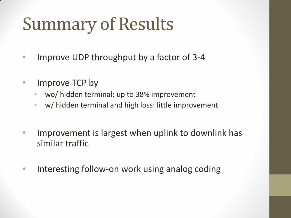
Summary of Results

• Improve UDP throughput by a factor of 3-4

• Improve TCP by • wo/ hidden terminal: up to 38% improvement

• w/ hidden terminal and high loss: little improvement

• Improvement is largest when uplink to downlink has

similar traffic

• Interesting follow-on work using analog coding

Reasons for Lower Improvement in TCP

• COPE introduces packet re-ordering

• Router queue is small smaller coding opportunity

• TCP congestion window does not sufficiently open up due to wireless losses

• TCP doesn’t provide fair allocation across different flows

Wireless and Mobile Communications - SJTUwang-xb/wireless_new/coursePages/course... · Existing...

Documents

Transcript of Wireless and Mobile Communications - SJTUwang-xb/wireless_new/coursePages/course... · Existing...