1

Winter measurements of oceanic biogeochemical parameters in the Rockall Trough

(2009-2012)

T. McGrath1, 2

, C. Kivimäe3, E. McGovern

1, R. R. Cave

2, and E. Joyce

1

1 Marine Institute, Rinville, Oranmore, Galway, Ireland

2 Earth and Ocean Science, School of Natural Sciences, National University of

Ireland, University Road, Galway, Ireland 3 National Oceanography Centre, University of Southampton Waterfront Campus

European Way, Southampton SO14 3ZH, United Kingdom

2

Abstract

This paper describes the sampling and analysis of biogeochemical parameters

collected in the Rockall Trough in January/February of 2009, 2010, 2011 and 2012.

Sampling was carried out across two transects, one southern and one northern transect

each year. Samples for dissolved inorganic carbon (DIC) and total alkalinity (TA)

were taken alongside salinity, dissolved oxygen and dissolved inorganic nutrients

(total-oxidised nitrogen, nitrite, phosphate and silicate) to describe the chemical

signatures of the various water masses in the region. These were taken at regular

intervals through the water column. The 2009 and 2010 data are available on the

CDIAC database.

Repository-Reference:

doi:10.3334/CDIAC/OTG.ROCKALL_TROUGH_2012

Available at:

http://cdiac.ornl.gov/ftp/oceans/Rockall_Trough/

Coverage: 52.8–56.2⁰N, 18.5–9 ⁰W

Location Name: Rockall Trough

Date/Time Start: 2009-02-05

Date/Time End: 2012-01-12

Table 1

Data Product Parameter Name Exchange File

Parameter Name

Exchange File

Flag Name

Units

Station STNNBR

Cast number CASTNO

Bottle number BTLNBR BTLNBR_FLAG_W

Year/month/day DATE

Time TIME

Latitude LATITUDE decimal degrees

Longitude LONGITUDE decimal degrees

Depth DEPTH meters

Pressure CTDPRS decibars

Temperature CTDTMP degrees Celsius

CTD Salinity CTDSAL CTDSAL_FLAG_W

Salinity SALNTY SALNTY_FLAG_W

CTD Oxygen CTDOXY CTDOXY_FLAG_W micromole kg−1

Dissolved oxygen OXYGEN OXYGEN_FLAG_W micromole kg−1

Dissolved inorganic silicate SILCAT SILCAT_FLAG_W micromole kg−1

Dissolved inorganic nitrate NITRAT NITRAT_FLAG_W micromole kg−1

Dissolved inorganic nitrite NITRIT NITRIT_FLAG_W micromole kg−1

Dissolved inorganic phosphate PHSPHT PHSPHT_FLAG_W micromole kg−1

Dissolved inorganic carbon TCARBN TCARBN_FLAG_W micromole kg−1

Total alkalinity ALKALI ALKALI_FLAG_W micromole kg−1

3

1. Introduction

Between February 2008 and August 2010 a pilot project to initiate research in ocean

carbon processes in Irish marine waters was carried out jointly by the National

University of Ireland, Galway (NUIG) and the Marine Institute, Ireland (MI). The

project titled “Increased Atmospheric CO2 on Ocean Chemistry and Ecosystems” was

carried out under the Sea Change strategy with the support of the Marine Institute and

the Marine Research Sub-Programme of the National Development Plan 2007–2013.

(O’Dowd et al., 2011). Through collaboration with annual MI winter surveys, a range

of biogeochemical parameters were measured across the Rockall Trough in January or

February of 2009, 2010, 2011 and 2012. The Rockall Trough plays an important role

in the global thermohaline circulation as it provides a pathway for warm saline waters

of the upper North Atlantic to reach the Nordic Seas. There is also a complex

interaction of a range of water masses in the Trough, each with different areas of

origin and histories (McGrath et al., 2012b) and therefore it is an important region in

ocean-climate research. The 2009 and 2010 data have recently been compared with

data measured in the Trough in the 1990s by the World Ocean Circulation Experiment

(McGrath et al., 2012a; McGrath et al., 2012b).

2. Data provenance

All surveys were carried out on the RV Celtic Explorer; see exact dates in Table 2.

While conductivity, temperature and depth (CTD) data are available for every station

in Figure 1, inorganic carbonate parameters were generally measured every second

station in 2009 and 2010. In 2011, only 5 surface carbonate samples were taken for

inter-laboratory comparison with samples analysed at Scripps Institute of

Oceanography, while in 2012 carbonate samples were taken at every station along the

southern transect. Salinity and nutrients were measured across both transects every

year. Stations were approximately 27 km apart, except for along the shelf edge where

there was greater horizontal sampling resolution.

4

Table 2 Details of surveys with number of chemistry samples taken on each.

Survey EXPOCODE Date DIC TA O2 NUT SAL

CE0903 45CE20090206 5-15 Feb 2009 64 64 144 133

CE10002 45CE20100209 5-17 Feb 2010 95 95 190 333 266

CE11001 3-10 Jan 2011 5 5 145 204 183

CE12001 5-12 Jan 2012 75 75 165 165

Figure 1 Station positions from the surveys CE0903 (Feb 2009), CE10002 (Feb

2010), CE11001 (Jan 2011) and CE12001 (Jan 2012). Stations with triangle symbols

are where carbonate parameters were measured. Note in CE11001 only surface

samples were taken, in other years samples were taken through the water column.

3. Methods and Quality Control Procedures

3.1 Hydrography

A Seabird CTD profiling instrument (SBE 911) with water bottles on a rosette was

used on each survey. Temperature and conductivity sensors were sent to Seabird

annually for calibration. On every survey there was a primary and secondary

temperature and conductivity sensor set on the CTD, which were compared to ensure

they match to a high level of precision. Also processed salinity sensor data were

5

compared with the discrete water samples analysed on a Guildline Portasal

salinometer (Model 8410A) at the MI. On every survey the sensor-laboratory

comparison resulted in an r-square greater than 0.999, therefore there were no

adjustments necessary on the salinity sensor data. An SB43 oxygen sensor was

deployed with the CTD, which was also calibrated annually with the manufacturer.

On surveys where oxygen samples were taken, the oxygen sensor data was calibrated

with the laboratory results.

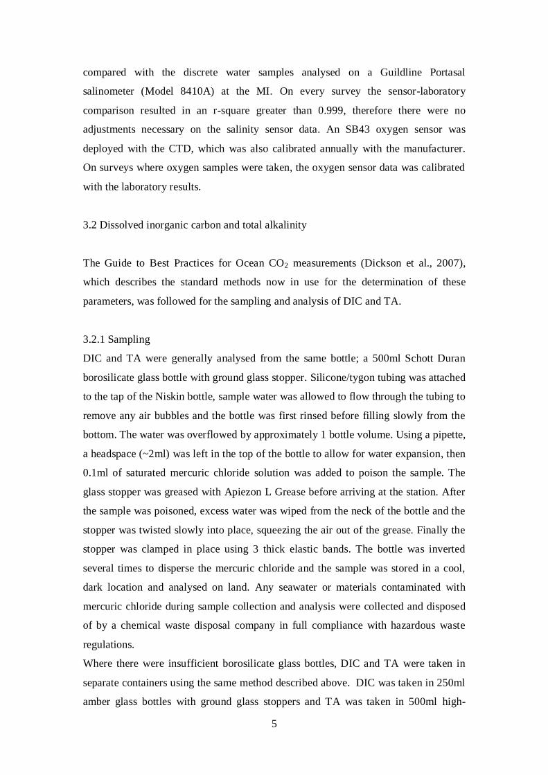
3.2 Dissolved inorganic carbon and total alkalinity

The Guide to Best Practices for Ocean CO2 measurements (Dickson et al., 2007),

which describes the standard methods now in use for the determination of these

parameters, was followed for the sampling and analysis of DIC and TA.

3.2.1 Sampling

DIC and TA were generally analysed from the same bottle; a 500ml Schott Duran

borosilicate glass bottle with ground glass stopper. Silicone/tygon tubing was attached

to the tap of the Niskin bottle, sample water was allowed to flow through the tubing to

remove any air bubbles and the bottle was first rinsed before filling slowly from the

bottom. The water was overflowed by approximately 1 bottle volume. Using a pipette,

a headspace (~2ml) was left in the top of the bottle to allow for water expansion, then

0.1ml of saturated mercuric chloride solution was added to poison the sample. The

glass stopper was greased with Apiezon L Grease before arriving at the station. After

the sample was poisoned, excess water was wiped from the neck of the bottle and the

stopper was twisted slowly into place, squeezing the air out of the grease. Finally the

stopper was clamped in place using 3 thick elastic bands. The bottle was inverted

several times to disperse the mercuric chloride and the sample was stored in a cool,

dark location and analysed on land. Any seawater or materials contaminated with

mercuric chloride during sample collection and analysis were collected and disposed

of by a chemical waste disposal company in full compliance with hazardous waste

regulations.

Where there were insufficient borosilicate glass bottles, DIC and TA were taken in

separate containers using the same method described above. DIC was taken in 250ml

amber glass bottles with ground glass stoppers and TA was taken in 500ml high-

6

density polyethylene (HDPE) bottles with screw caps. The individual TA samples

were not poisoned with mercuric chloride.

3.2.2 Analysis

DIC was measured on a VINDTA-3C (Versatile Instrument for the Determination of

Titration Alkalinity) system (Mintrop et al., 2000) with UIC coulometer. A known

volume of sample is acidified with phosphoric acid in order to transfer all dissolved

inorganic carbon to CO2 and the resulting CO2, forced out of the sample using

nitrogen as a carrier gas, is titrated coulometrically (Johnson et al., 1987; Johnson et

al., 1993).

TA was analysed by potentiometric titration with 0.1M hydrochloric acid, also on the

VINDTA 3C. During the titration the bases in the TA definition (Dickson, 1981) are

transferred to their acidic forms and the titration is monitored by a pH electrode that

measures the electromotive force (emf). The process is controlled by the LabVIEWTM

software and the endpoint is determined by the change in pH against the volume of

acid added to the solution. The result of the titration is evaluated with curve fitting

(Mintrop et al., 2000).

3.2.3 Quality Control

The accuracy of both DIC and TA analysis was ensured by analysing duplicate

Certified Reference Materials (CRMs) before every batch of samples. CRMs were

provided by A. Dickson, Scripps Institution of Oceanography, USA (Dickson et al.,

2003). If many samples (>10) were run in a single batch, another duplicate CRM was

run at the end of the day. The mean of the measured CRM results was used to

calculate a CRM correction factor to adjust DIC and TA sample results for any offset

in the VINDTA.

CRM correction factor = assigned value / measured value

Sample results were then multiplied by the daily correction factors. The CRM results

are shown in Figure 2. It is unclear why the TA CRMs for Batch 102 used for

CE10002 had a slightly larger offset than other batches. Vertical profiles of final TA

concentrations from this survey were cross-checked with TA profiles from CE12001

and two WOCE surveys in the same region (McGrath et al., 2012). All suggest that

there is no problem/offset in the TA results generated from this batch. By using the

7

CRM correction factor, results were corrected for the larger offset in the instrument

during this time. Duplicate samples from the same bottle were run every second

sample, while duplicate bottles were taken for 5-10% of the total sample number from

each survey. The accuracy and precision of the measurements was calculated as the

average and standard deviation, respectively of the differences between duplicate

samples, Table 3.

Figure 2 DIC and TA CRM measured values plotted against certified values for each

of the surveys. Dashed lines indicate a new survey.

Table 3 Accuracy and precision of DIC and TA in µmol kg-1

for each of the surveys,

calculated as the average and standard deviation, respectively of the differences

between duplicate samples, where n is the number of duplicate samples.

Accuracy DIC

Precision DIC

Accuracy TA

Precision TA

n

CE0903 2 2 1 1 64

CE10002 3 2 1 1 60

CE11001 1 1 2 2 4

CE12001 2 1 2 2 43

1900 1925 1950 1975 2000 2025 2050 2075 2100 2125 2150

DIC

(µ

mo

l kg-

1)

Cert. CRM DIC

Meas. CRM DIC

CE0903 CE10002 CE11001 CE12001

B#97

B# 99

B# 102 B# 104 B# 120

2130

2180

2230

2280

2330

2380

2430

2480

2530

TA (

µm

ol k

g-1

)

Cert. CRM TA

Meas. CRM TA

B# 97 B# 102

CE0903 CE10002 CE11001 CE12001

B# 104 B# 120

B# 99

8

DIC and TA Storage Experiment

A storage experiment was carried out to investigate if storing samples for a prolonged

length of time had an effect on the DIC and TA concentration. On May 21st 2010,

twenty-six 500ml Schott Duran bottles were filled with water taken from 448m deep

along the shelf edge (10.0322ºW, 55.2565ºN). All bottles were filled by the author

(TMG), while a colleague poisoned, greased and sealed the bottles. Six 250ml glass

(not-borosilicate) bottles, used for DIC only, were also tested to ensure these bottles

did not affect the stored samples differently than the Schott Duran bottles. All samples

were poisoned with mercuric chloride, stored at 4ºC in a dark fridge until they were

analysed. The first set of samples (T=0) was run on the 29th

May 2010 and a new set

of samples was run monthly for the first 7 months (with one exception), with

subsequent analysis every 2-3 months. A duplicate of every bottle was run, and the

final result for each bottle below (Figure 3) is an average of the duplicate values.

The average DIC at T=0 was 2143µmol kg-1

(analysed from 4 duplicate sample

bottles). The average DIC over the first full year of storage was 2142µmol kg-1

, and

variation around the mean is less than ±3µmol kg-1

. Both Schott Duran and soft glass

bottles had similar concentrations after a year. There was greater variability in DIC

concentrations in the second year of storage, results from one month (July 2011) were

discarded as concentrations were over 10µmol kg-1

below the mean.

The average TA at T=0 was 2331µmol kg-1

, and remained constant for the 26 months

of storage, with variation less than ±2µmol kg-1

around the mean. Results from one

month (June 2010) were discarded as concentrations were 8µmol kg-1

above all other

months and appear to be a one-off error.

Results indicate while TA samples can be stored for at least two years, DIC samples

should be analysed within one year of sampling. All samples collected in the Rockall

Trough were analysed well within one year of sampling.

9

Figure 3 Average monthly (from at least 2 sample bottles) DIC and TA concentrations

over 2 years of storage. The mean and standard deviations for DIC were based on the

first year of storage when concentrations were within ±3µmol kg-1

around the mean,

while both years of storage results were used for TA as they were all within ±2µmol

kg- of the mean.

Cross validation of DIC and TA analysed at Scripps Institution of Oceanography

In the survey CE11001 across the Rockall Trough in January 2011, a batch of surface

DIC and TA samples was sent to Scripps Institution of Oceanography (SIO), USA,

for analysis. Five duplicates of these samples were analysed by the author (TMG) at

NUIG. DIC and TA concentrations from NUIG were within ±3.1µmol kg-1

and

±1.3µmol kg-1

, respectively, of those analysed at SIO.

3.3 Dissolved inorganic nutrients

3.3.1 Sampling

All equipment involved in the sampling and filtration of nutrient samples were acid-

cleaned in 10% hydrochloric acid prior to sampling (Grasshoff, 1999). Water for

nutrient samples was collected from the Niskin bottle in 1L HDPE bottles. The 1L

2132

2135

2138

2141

2144

2147

2150

Apr-10 Oct-10 May-11 Nov-11 Jun-12

DIC

(µm

ol k

g-1)

DIC mean DIC +2 SD -2 SD +3 SD -3 SD

2328

2329

2330

2331

2332

2333

2334

2335

Apr-10 Oct-10 May-11 Nov-11 Jun-12

TA (µ

mo

l kg-

1) TA

mean TA

-2 SD

+2 SD

+3 SD

-3 SD

10

bottles were first rinsed 3 times with sample water before filling. The sample was

filtered through a 0.40m polycarbonate filter and the filtrate was poured into two

50ml polypropylene tubes. The tubes were immediately frozen upright at -20ºC and

analysed on land.

3.3.2 Analysis

Seawater samples were analysed for total oxidised nitrogen (TOxN), nitrite, silicate

and phosphate on a Skalar San++

Continuous Flow Analyser at the Marine Institute

(Grasshoff, 1999). The Skalar San++

System uses automatic segmented flow analysis

where a stream of reagents and samples, segmented with air bubbles, is pumped

through a manifold to undergo treatment such as mixing and heating before entering a

flow cell to be detected. The sample is pumped into the system and split into 4

channels where it is mixed with reagents. The reagents act to develop a colour, which

is measured as an absorbance through a flow cell at a given wavelength.

TOxN

The Skalar method for the determination of TOxN is based on Greenberg et al.

(1980), ISO 13395 (1996), Navone (1964) and Walinga et al. (1989). The sample is

first buffered at a pH of 8.2, with a buffer reagent made of ammonium chloride and

ammonium hydroxide solution, and is then passed through a column containing

granulated copper-cadmium to reduce nitrate to nitrite. The nitrite, originally present

plus reduced nitrate, is determined by diazotizing with sulfanilamide and coupling

with N-(1-naphthyl) ethylenediamine dihydrochloride to form a strong reddish-purple

dye which is measured at 540nm.

Nitrite

The Skalar method for the determination of nitrite is based on EPA (1974), Greenberg

et al. (198) and ISO 13395 (1996), where the diazonium compounds formed by

diazotizing of sulfanilamide by nitrite in water under acidic conditions (due to

phosphoric acid in the reagent) is coupled with N-(1-naphthyl) ethylenediamine

dihydrochloride to produce a reddish-purple colour which is measured at 540nm.

Silicate

The Skalar method for the determination of silicate is based on Babulak and

Gildenberg (1973), ISO-16264 (2002) and Smith and Milne (1981). The sample is

11

acidified with sulphuric acid and mixed with an ammonium heptamolybdate solution

forming molybdosilicic acid. This acid is reduced with L(+)ascorbic acid to a blue

dye, which is measured at 810nm. Oxalic acid is added to avoid phosphate

interference.

Phosphate

The Skalar method for the determination of phosphate is based on Boltz and Mellon

(1948), Greenberg et al. (1980), Walinga et al. (1989) and ISO 15681-2 (2003), where

ammonium heptamolybdate and potassium antimony(III) oxide tartrate react in an

acidic medium (with sulphuric acid) with diluted solutions of phosphate to form an

antimony-phospho-molybdate complex. This complex is reduced to an intensely blue-

coloured complex by L(+)ascorbic acid and is measured at 880nm.

Based on the daily calibration standards, concentrations of nutrients can be quantified

up to the maximum calibration standard concentration. If sample concentrations fall

above this range (Table 4), they must be diluted with artificial seawater.

Table 4 Limit of detection (LOD), limit of quantification (LOQ), both in μmol l-1

, and

uncertainty of measurement (UCM) for the nutrient analysis. The ranges given are the

linear calibration ranges, concentrations that fall above these are diluted into the linear

range.

LOD LOQ UCM Ranges

TOxN 0.02 0.26 2.3% LOQ – 15

Nitrite 0.01 0.04 6.7% LOQ – 1.5

Silicate 0.03 0.38 0.5% LOQ – 15

Phosphate 0.01 0.16 1.3% LOQ – 1.5

3.3.3 Nutrients Quality Control

The accuracy of the nutrient analysis was ensured by running Eurofins CRMs

(http://www.eurofins.dk/dk/milj0/reference-materialer.aspx) with every batch of

samples, which must fall within specified limits within a standard deviation of 2. The

system is also calibrated in every run using seven calibration standards made up daily

in the laboratory. A replicate of every sample is analysed and the relative percent

12

difference (RPD: difference between the two values / mean * 100) of the results

greater than the limit of quantification should be ≤ 10.

To assess the accuracy of the nutrient methods and procedures the MI participates in

the QUASIMEME laboratory quality control programme (www.quasimeme.org). Test

materials, analysed twice a year, have a large range of concentrations from below the

detection limit to high concentrations that have to be diluted. The laboratory

performance is expressed with a z-score where |z| < 2 is considered acceptable, where

z is the difference between the laboratory result and the assigned value divided by the

total error (Cofino and Wells, 1994). Between Oct 2008 and May 2012 the MI

participated in 8 rounds of QUASIMEME proficiency testing scheme exercises (51

samples) for nutrients in the marine environment. The average z-score for all nutrients

was <0.5, see Figure 4. The MI is accredited to ISO 17025 for nutrient analysis in

seawater and is audited annually by the Irish National Accreditation Board, INAB.

Figure 4 z-scores of 8 QUASIMEME rounds of nutrients in the marine environment

between October 2008 and May 2012, where the green dashed lines indicate a z-score

of 2. The dashed black line at a z score of ±3 designates unsatisfactory performance.

Most of the Quasimeme samples were in the range of oceanic values measured in the

Rockall Trough.

-3

-2

-1

0

1

2

3

Oct

-08

Ap

r-0

9

No

v-09

Jun

-10

Jan

-11

Au

g-1

1

Mar

-12

TOxN

-3

-2

-1

0

1

2

3

Oct

-08

Ap

r-0

9

No

v-0

9

Jun

-10

Jan

-11

Au

g-1

1

Mar

-12

Nitrite

-3

-2

-1

0

1

2

3

Oct

-08

Ap

r-09

No

v-09

Jun

-10

Jan

-11

Au

g-11

Mar

-12

Phosphate

-3

-2

-1

0

1

2

3

Oct

-08

Ap

r-09

No

v-09

Jun

-10

Jan

-11

Au

g-11

Mar

-12

Silicate

13

3.4 Salinity

3.4.1 Sampling

Salinity samples were collected in clear glass salinity bottles with plastic screw caps.

The bottle was first rinsed three times with the sample water before filling up to the

shoulder of the bottle. The neck of the bottles was dried well with clean kim wipes to

prevent salt crystals forming on the top. A plastic insert was then placed into the

bottle to produce a tight seal to prevent evaporation, followed by closing the bottle

with the screw cap. Samples were stored upright at room temperature.

3.4.2 Analysis

Salinity was analysed on a Guildline Portasal Salinometer at the MI, where 4

electrode conductivity cells suspended in a temperature-controlled bath, measure the

conductivity of the sample. The conductivity is related to salinity by calibration from

a known standard. Two consecutive conductivity readings within 0.00002 units of

each other must be taken before the salinity can be recorded. The temperature of the

salinometer water bath must be set and stabilized to ~1-2ºC above ambient room

temperature and samples must reach room temperature before analysis.

3.4.3 Salinity Quality Control

IAPSO seawater standards from OSIL (Ocean Scientific International Ltd) are used to

calibrate the instrument daily and run as CRMs with every batch of samples. A P-

series IAPSO standard (salinity ~35) is used to calibrate the system and is run every 4

hours during analysis and at the end of the days’ analysis. DI water (salinity= 0), a

10L IAPSO standard (salinity ~10) and a 38H IAPSO standard (salinity ~38) are

tested at the beginning of every batch of samples. P Series standards (salinity ~35)

should fall within an allowable error of +0.003. The average z-score over 8 rounds of

QUASIMEME proficiency testing scheme exercises for salinity between Oct 2008

and May 2012 was 0.36, see Figure 5. The MI is also accredited to ISO 17025 for

salinity analysis in seawater and is audited by the Irish National Accreditation Board,

INAB.

14

Figure 5 z-scores of 8 QUASIMEME rounds of salinity in the marine environment

between October 2008 and May 2012, where the green dashed lines indicate a z-score

of 2. The dashed black line at a z score of ±3 designates unsatisfactory performance.

3.5 Dissolved oxygen

Dissolved oxygen (D.O.) samples were collected and analysed as per the standard

operating procedure of Dickson (1995).

3.5.1 Sampling

D.O. was the first parameter to be sampled from the CTD, with deepest samples

drawn first, and collected in 250ml iodine bottles with plastic stoppers. All bottle-

stopper pairs are individually calibrated and exact bottle volumes are used in final

oxygen calculations. The bottle was filled from the bottom using silicone/tygon

tubing, care was taken to minimize bubbles when filling and the water was

overflowed by 3 flask volumes. Two millimetres of the pickling reagents, MnCl2 (no.

1) and NaOH/NaI (no. 2), were added immediately to the sample, before carefully

inserting the stopper and inverting the bottle several times. After the precipitate had

settled at least half way, the bottle was shaken again. Samples were then stored in a

cool dark location until titration, which was mostly carried out within 12 hours of

sampling.

3.5.2 Analysis

Oxygen samples were analysed using a modified Winkler method (Dickson, 1995),

where the titration is carried out in the sample bottle. The sample is first acidified with

sulphuric acid (H2SO4) to a pH between 1 and 2.5, which dissolves the hydroxide

precipitates, and iodide ions added by reagent no.2 are oxidised to iodine by the

manganese (III) ions, which are reduced to Mn(II) ions in the process. In the final

-3

-2

-1

0

1

2

3

Oct

-08

Ap

r-0

9

No

v-0

9

Jun

-10

Jan

-11

Au

g-1

1

Mar

-12

Salinity

15

step, the iodine is reduced to iodide by titration with sodium thiosulfate, the amount of

iodine generated, which is equivalent to the amount of oxygen in the sample, is

determined by the amount of thiosulfate required to reach the endpoint. A Metrohm

848 Titrino Plus, with a Metrohm combined Pt electrode was used to determine the

endpoint, i.e. potentiometric endpoint determination, measuring the change in redox

potential of the sample, which reaches a minimum at the endpoint (Furuya and

Harada, 1995). This method of determination was also used effectively by numerous

WOCE cruises in the Atlantic and Pacific Oceans, and also on some Hawaii Ocean

Time Series (HOT) cruises

(http://www.soest.hawaii.edu/HOT_WOCE/).

3.5.3 Oxygen Quality Control

Before titration of the samples, duplicate reagent blanks were determined and

duplicate standardization of the sodium thiosulfate titrant was carried out. The reagent

blank should ideally be less than 0.01ml, while the duplicate thiosulfate

standardization should typically fall within 0.002ml of each other (Dickson, 1995).

Standardization of the thiosulfate is carried out in precisely the same conditions that

the samples are analysed under so that any iodine lost through the volatilization or

gained by the oxidation of iodide while analysing the seawater samples is

compensated for with similar errors occurring during the standardization procedure

(Knapp et al., 1989). Precision of the samples is estimated by running duplicate

samples every 10-15 samples.

4. Data access

The 2009 and 2010 datasets are currently available on CDIAC database

(http://cdiac.ornl.gov/ftp/oceans/Rockall_Trough/), and discussed in McGrath et al.

(2012a) and McGrath et al. (2012b). The 2011 and 2012 datasets are currently being

quality checked and will be submitted to CDIAC once this is completed.

Acknowledgements

We would like to thank our colleagues at the Marine Institute, Ireland and at the

National University of Ireland, Galway that have contributed to the data collection

both at sea and in the laboratory. We also thank the crew of the Celtic Explorer who

assisted us in our data collection across the Rockall Trough.

16

References

Babulak, S.W., Gildenberg, L., 1973. Automated determination of silicate and

carbonates in detergents. Journal of the American Oil Chemists’ Society, 5,

296-299.

Dickson, A.G., 1981. An exact definition of total alkalinity and a procedure for the

estimation of alkalinity and total inorganic carbon from titration data. Deep

Sea Research Part A. Oceanographic Research Papers, 28(6): 609-623.

Dickson, A.G., 1995. Determination of dissolved oxygen in sea water by Winkler

titration. WOCE Operations Manual. Part 3.1.3 Operations & Methods, WHP

Office Report WHPO 91-1.

Dickson, A.G., Afghan, J.D. and Anderson, G.C., 2003. Reference materials for

oceanic CO2 analysis: a method for the certification of total alkalinity. Marine

Chemistry, 80(2-3): 185-197.

Dickson, A.G., Sabine, C.L. and Christian, J.R., 2007. Guide to best practices for

ocean CO2 measurements. PICES Special Publication 3: 1-191.

EPA, 1974. Method of chemical analysis of water and wastes. Off Technological

Transfer, Environmental Protection Agencym Washington D.C.

Furuya, K. and Harada, K., 1995. An Automated Precise Winkler Titration for

Determining Dissolved Oxygen on Board Ship. Journal of Oceanography, 51:

375-383.

Grasshoff, K., Ehrhardt, M., Kremling, K. and Almgren, T., 1999. Methods of

seawater analysis. Third Edition. Wiley-VCH.

Greenberg, A.E., Jenkins, D. and Connors, J.J., 1980. Standard Methods for the

Examination of Water and Wastewater. APHA-AWWA-WPCF.

ISO 13395 (1996). Determination of nitrite nitrogen and nitrate nitrogen and the sum

of both by flow analysis (CFA) and spectrometric detection.

ISO 15681-2, 2003. Determination of ortho phosphate and total phosphorus conents

by flow analysis, Part 2: Method by continuous flow analysis (CFA).

ISO 16264, 2002. Determination of soluble silicals by CFA and photometric

detection.Johnson, K.M., Sieburth, J.M., Williams, P.J.l. and Brändström, L.,

1987. Coulometric total carbon dioxide analysis for marine studies:

Automation and calibration. Marine chemistry, 21: 117-133.

Johnson, K.M., Wills, K.D., Butler, D.B., Johnson, W.K. and Wong, C.S., 1993.

Coulometric total carbon dioxide analysis for marine studies: maximizing the

performance of an automated gas extraction system and coulometric detector.

Marine chemistry, 44: 167-187.

Knapp, G.P., Stalcup, M.C. and Stanley, R.J., 1989. Dissolved oxygen measurements

in sea water at the Woods Hole Oceanographic Institution.

McGrath, T., Kivimae, C., Tanhua, T., Cave, R.R. and McGovern, E., 2012a.

Inorganic carbon and pH levels in the Rockall Trough 1991-2010. Deep Sea

Research Part I: Oceanographic Research Papers, 68(0): 79-91.

McGrath, T., Nolan, G. and McGovern, E., 2012b. Chemical characteristics of water

masses in the Rockall Trough. Deep Sea Research Part I: Oceanographic

Research Papers, 61(0): 57-73.

Mintrop, L., Pérez, F.F., Gonzalez-Dávila, M., Santana-Casiano, J.M. and Körtzinger,

A., 2000. Alkalinity determination by potentiometry: intercalibration using

three different methods. Ciencias Marinas, 26(1): 23-37.

Navone, R., 1964. Proposed method for nitrate in potable waters. American Journal

Water Work Association, 56, 781-783.

17

O’Dowd, C., Cave, R., McGovern, E., Ward, B., Kivimae, C., McGrath, T., Stengel,

D. and Westbrook, G., 2011. Impacts of Increased Atmospheric CO2 on

Ocean Chemistry and Ecosystems.

Smith, J.D., Milne, P.J., 1981. Spectrophotometric determination of silicate in natural

waters by formation of α-molybdosilicic acid and reduction with tin(IV)-

ascorbic acid-oxalic mixture. Analytica Chimica Acta 123, 263-270.

Walinga, I., van Vark, W. Houba, V.J.G., van der Lee, J.J., 1989. Plant analysis procedure, Part

7. Department of Soil Science and Plant Nutrition, Wageningen Agricultural University,

197-200.