Winners and Losers from Trade Reform in Morocco...Winners and Losers from Trade Reform in Morocco...
38
Reference: Francois Bourguignon, Luiz Pereira da Silva and Maurizio Bussolo (eds), The Impact of Economic Policies on Poverty and Income Distribution: Advanced Evaluation Techniques and Tools. Oxford: Oxford University Press, 2008. Winners and Losers from Trade Reform in Morocco Martin Ravallion and Michael Lokshin 1 Development Research Group, World Bank Abstract: We use Morocco’s national survey of living standards to measure the short-term welfare impacts of prior estimates of the price changes attributed to various agricultural trade reform scenarios for de-protecting cereals — the country’s main foodstaple. We find small impacts on mean consumption and inequality in the aggregate. There are both winners and losers and (contrary to past claims), the rural poor are worse off on average after de-protection. We decompose the aggregate impact on inequality into a “vertical” component (between people at different pre-reform welfare levels) and a “horizontal” component (between people at the same pre-reform welfare). There is a large horizontal component, which dominates the vertical impact of full de-protection. The diverse impacts reflect a degree of observable heterogeneity in consumption behavior and income sources, with implications for social protection policies. 1 This paper was originally written as a background paper to the report: Kingdom of Morocco: Poverty Report: Strengthening Policy by Identifying the Geographic Dimension of Poverty, Report No. 28223-MOR, World Bank, 2004. The authors are grateful to Touhami Abdelkhalek, Maurizio Bussolo, Jennie Litvack, Sherman Robinson, Hans Timmer and seminar participants at the World Bank for comments on an earlier version and to Rachid Doukkali for help in using the results of his CGE analysis. These are the views of the authors, and should not be attributed to the World Bank or any affiliated organization.
Transcript of Winners and Losers from Trade Reform in Morocco...Winners and Losers from Trade Reform in Morocco...

Reference: Francois Bourguignon, Luiz Pereira da Silva and Maurizio Bussolo (eds), The Impact of
Economic Policies on Poverty and Income Distribution: Advanced Evaluation Techniques and Tools.
Oxford: Oxford University Press, 2008.
Winners and Losers from Trade Reform in Morocco
Martin Ravallion and Michael Lokshin1
Development Research Group, World Bank
Abstract: We use Morocco’s national survey of living standards to measure the
short-term welfare impacts of prior estimates of the price changes attributed to
various agricultural trade reform scenarios for de-protecting cereals — the
country’s main foodstaple. We find small impacts on mean consumption and
inequality in the aggregate. There are both winners and losers and (contrary to
past claims), the rural poor are worse off on average after de-protection. We
decompose the aggregate impact on inequality into a “vertical” component
(between people at different pre-reform welfare levels) and a “horizontal”
component (between people at the same pre-reform welfare). There is a large
horizontal component, which dominates the vertical impact of full de-protection.
The diverse impacts reflect a degree of observable heterogeneity in consumption
behavior and income sources, with implications for social protection policies.
1 This paper was originally written as a background paper to the report: Kingdom of Morocco:
Poverty Report: Strengthening Policy by Identifying the Geographic Dimension of Poverty, Report No.
28223-MOR, World Bank, 2004. The authors are grateful to Touhami Abdelkhalek, Maurizio Bussolo,
Jennie Litvack, Sherman Robinson, Hans Timmer and seminar participants at the World Bank for
comments on an earlier version and to Rachid Doukkali for help in using the results of his CGE analysis.
These are the views of the authors, and should not be attributed to the World Bank or any affiliated
organization.

2
1. Introduction
As a water-scarce country, Morocco does not have much natural advantage in the
production of water-intensive crops such as most cereals, including wheat, which is used to
produce the country’s main food staples. The desire for aggregate self-sufficiency in the
production of food staples has led in the past to governmental efforts to foster domestic cereal
production, even though cereals can be imported more cheaply. Since the 1980s, cereal
producers have been protected by tariffs on imports as high as 100%.
There have been concerns that the consequent reallocation of resources has hurt
consumers and constrained the growth of production and trade. Reform to the current incentive
system for cereals has emerged as an important issue on the policy agenda for Morocco (World
Bank, 2003). The major obstacles to reform stem from concerns about the impacts on household
welfare, particularly for the poor. There has been very little careful research into who will gain
and who will lose from such reforms.
Nonetheless, there has been much debate about the equity implications. It is widely
agreed that urban consumers will gain from lower cereal prices. More contentious are the
impacts in (generally poorer) rural areas. Defenders of the existing protection system have
argued that there will be large welfare losses to the rural economy from trade reform. Critics
have argued against this view, claiming that the bulk of the rural poor tend to be net consumers,
and so lose out from the higher prices due to trade protection. They argue that the rural poor are
likely to gain from the reform, while it will be the well off in rural areas, who tend to be net
producers, who will lose; see for example, Abdelkhalek (2002) and World Bank (2003).
This paper studies the household welfare impacts of the relative price changes induced by
specific trade policy reform scenarios for cereals in Morocco. Past analyses of the welfare
impacts have been highly aggregated, focusing on just one or a few categories of households.
Here we estimate impacts across 5,000 sampled households in the Morocco Living Standards
Survey for 1998/99. This allows us to provide a detailed picture of the welfare impacts, so as to
better inform discussions of the social protection policy response to trade liberalization.
Past approaches to studying the welfare impacts of specific trade reforms have tended to
be either partial equilibrium analyses, in which the welfare impacts of the direct price changes
due to tariff changes are measured at household level, or general equilibrium analyses, in which

3
second-round responses are captured in a theoretically consistent way but with considerable
aggregation across household types. In general terms, the economics involved in both
approaches is well known. And both approaches have found numerous applications.2
We combine these two approaches. In particular, the price changes induced by the trade-
policy change are simulated from a general equilibrium analysis done for a Joint Government of
Morocco and World Bank Working Group. We take the methods and results of that analysis as
given and carry them to the Moroccan Living Standards survey. Our approach respects the
richness of detail available from a modern integrated household survey, allowing us to go well
beyond the highly aggregative types of analysis one often finds. We not only measure expected
impacts across the distribution of initial levels of living, but we also look at how they vary by
other characteristics, such as location. We are thus able to provide a reasonably detailed “map”
of the predicted welfare impacts by location and socio-economic characteristics.
In studying the distributional impacts of trade reform we make a distinction between the
“vertical impact” and “horizontal impact.” The former concerns the way the mean impacts vary
with level of pre-reform income; how does the reform affect people at different pre-reform
incomes? The horizontal impact relates to the disparities in impact between people at the same
pre-reform income. As argued in Ravallion (2004), many past discussions of the distributional
impacts of trade and other economy-wide reforms have tended to focus more on the vertical
impacts, analogously to standard practices in studying the “benefit incidence” of tax and
spending policies. However, as we will demonstrate here, this focus may well miss an important
component of a policy’s distributional impact, arising from the horizontal dispersion in impacts
at given pre-reform incomes. We show how the impact of a policy on a standard inequality
measure can be straightforwardly decomposed into its vertical and horizontal components. The
former tells us how much of the change in total inequality can be accounted for by the way in
which mean impacts conditional on pre-reform income vary with the latter. If there is no
difference in the proportionate impact by level of income then the vertical component is zero.
The horizontal component tells us the contribution of the deviations in impacts from their
conditional means. Only when the impact of the reform is predicted perfectly by pre-reform
2 See the surveys by McColluch et al., (2001) and Hertel and Reimer (2004). A number of chapters
in Bourguignon and Pareira da Silva (2003, Part 2) describe alternative approaches using general
equilibrium models.

4
income will the horizontal component be zero. We study the relative importance of these two
components of our predicted distributional impact of trade reform in Morocco.
The following section discusses our approach in general terms; the Appendix provides
more detail. Section 3 presents our results in detail, while section 4 reviews the main findings.
2. Measuring and explaining the welfare impacts of reform using micro data
We use pre-existing estimates of the household-level welfare impacts of the price changes
generated by a Computable General Equilibrium (CGE) model. The CGE analysis generates a
set of price changes; these embody both the direct price effects of the trade-policy change and
indirect effects on the prices of both traded and non-traded goods once all markets respond to the
reform. Standard methods of first-order welfare analysis are used to measure the gains and
losses at household level. Note that this approach is sequential rather than integrated. In other
words, there is no feedback from the empirical analysis of welfare impacts to the CGE analysis.
The alternative approach is to fully integrate the CGE analysis with the household-level data;
see, for example, Cockburn (2003).
Our focus here is very much on the short-term welfare impacts. In keeping with the
limitations of the general equilibrium analysis on which we draw, our approach does not capture
the dynamic effects of trade reform through labor market adjustment and technological
innovation. Nor does it capture potential gains to the environment.3
The specifics of our approach to estimating welfare impacts at the household level are
outlined in the Appendix, and we only summarize the salient features here.4 Each household has
preferences over consumption and work effort represented by a standard utility function. The
household is assumed to be free to choose its preferred combinations of consumptions and labor
supplies subject to its budget constraint. The household also owns a production activity
3 Though it is not a subject of the present analysis, arguments are also made about adverse
environmental impacts arising from the expansion of protected cereal production into marginal areas, It is
claimed that scarce water resources have also been diverted into soft wheat production. For further
discussion see World Bank (2003). 4 There are many antecedents of our approach in the literatures on both tax reform and trade
reform, though there are surprisingly few applications to point to in the ex ante assessment of actual
reform proposals. For another example see Chen and Ravallion (2004). Hertel and Reimer (2004)
provide a useful overview of the strengths and weaknesses of alternative approaches to assessing the
welfare impacts of trade-policies, including references to empirical examples for developing countries.

5
generating a profit that depends on a vector of supply prices and wages. The indirect utility
function of the household (giving the maximum utility attainable given the constraints) also
depends on prices and wages.
We take the predicted price impacts from the CGE model as given for the analysis of
household-level impacts. In measuring the impacts we are constrained of course by the data,
which do not include prices and wages. However, this limitation does not matter to calculating a
first-order approximation to the welfare impact in a neighborhood of the household’s optimum
(as outlined in the Appendix). This gives us a measure of the monetary value of the gain to
household i denoted ig . This is obtained by adding up the proportionate changes in all prices
weighted by their corresponding expenditure or revenue shares. The weight for the proportionate
change in the j’th selling price is the revenue (selling value) from household production activities
in sector j; similarly the consumption expenditure shares are the (negative) weights for demand
price changes while earnings provide the weights for changes in the wage rates. The difference
between revenue and expenditure gives (to a first-order approximation) the welfare impact of an
equi-proportionate increase in the price of a given commodity. In the specific model we will use
(as discussed later), real wage rates are fixed. We discuss likely implications of relaxing this
assumption in section 3.5.
Notice that by using the calculus in deriving the welfare gains, ig for i=1,..,n, we are
implicitly assuming small changes in prices. Relaxing this requires more information on the
structure of the demand and supply system; see for example Ravallion and van de Walle (1991).
This would entail considerable further effort, and the reliability of the results will be
questionable given the aforementioned problem of incomplete price and wage data. For the
same reason, we will have little choice but to largely ignore geographic differences in the prices
faced, or in the extent to which border price changes are passed on locally.
Having estimated the impacts at household level, we can study how they vary with pre-
reform welfare, and what impact the reform has on poverty and inequality. Let iy denote the
pre-reform welfare per person in household i while iii gyy * is its post-reform value, where
ig is the gain to household i. (Ideally, iy will be an exact money-metric of utility, though in
practice it can be expected that it is an approximation given omitted prices or characteristics.)
The distribution of post-reform welfare levels is **2
*1 ,..., nyyy . By comparing standard summary

6
measures of poverty or inequality for this distribution with those for the pre-reform distribution,
nyyy ,..., 21 , we can assess overall impacts.
Of obvious interest is to see how the gains vary with pre-reform welfare. Is it the poor
who tend to gain, or is it middle-income groups or the rich? However, it is important to
recognize that the assignment of impacts to the pre-reform distribution is very unlikely to be a
degenerate distribution, with no distribution of its own. There will almost certainly be a
dispersion in impact at given pre-reform welfare. This will arise from (observable and
unobservable) heterogeneity in characteristics and prices. It could also arise from errors in the
welfare measure. Averaging across the distribution of impacts at given pre-reform welfare, one
can calculate the conditional mean impact given by:
)( iiici yygEg (1)
where the expectation is formed over the conditional distributions of impacts. By including a
subscript i in the expectations operator in (1), we allow the possibility that the horizontal
dispersion in impacts is not identically distributed. In our empirical implementation, equation
(1) will be estimated using a non-parametric regression.
Taking these observations a step further, we can think of the overall impact on inequality
as having both vertical and horizontal components.5 This is straightforward for the Mean Log
Deviation (MLD) — an inequality measure known to have a number of desirable features.6 The
mean log deviation defined on the distribution of post-reform welfares **2
*1 ,..., nyyy is given by:
n
iiyy
nI
1
*** )/ln(1
(2)
where nyyn
ii /
1
**
is mean post-reform welfare. Similarly,
n
iiyy
nI
1
)/ln(1
(3)
5 Antecedents to this type of decomposition can be found in the literature on horizontal equity in
taxation. In the context of assessing a tax system, Auerbach and Hassett (2002) show how changes in an
index of social welfare can be decomposed into terms reflecting changes in the level and distribution of
income, the burden and progressivity of the tax system and a measure of the change in horizontal equity. 6 For further discussion of the MLD see Bourguignon (1979) and Cowell (2000). MLD is a
member of the General Entropy class of inequality measures.

7
is the pre-reform MLD. (In both (2) and (3) it is assumed that 0iy and 0* iy for all i.)
Thus I*- I is the change in inequality attributable to the reform. The proposed decomposition of
the overall change in inequality can then be written as:
n
i ii
ici
n
i ici
n
i ii yg
yg
nyg
yg
nyg
yg
nII
111
*
/1
/1ln
1
/1
/1ln
1
/1
/1ln
1 (4)
vertical component + horizontal component
The vertical component is the contribution to the change in total inequality (I*- I ) of the way in
which mean impacts vary with pre-reform welfare levels. If there is no difference in the
proportionate impact by level of welfare ( ygyg ici // for all i) then the vertical component is
zero. The horizontal component is the contribution of the deviations in impacts from their
conditional means. If the impact of the reform is predicted perfectly by pre-reform welfare
( cii gg for all i) then the horizontal component is zero.
The above decomposition is largely of descriptive interest. There are no immediate
policy implications, though finding that the horizontal component is large could well motivate
greater effort by policy makers to understand what characteristics of households are associated
with the differences in impacts found empirically.
To help in that task, we can go a step further and try and explain the differences in
impacts in terms of observable characteristics of potential relevance to social protection policies.
The way we have formulated the problem of measuring welfare impacts above allows utility and
profit functions to vary between households at given prices. To try to explain the heterogeneity
in measured welfare impacts we can suppose instead that these functions vary with observed
household characteristics. We allow the characteristics that influence preferences over
consumption ( ix1 ) to differ from those that influence the profits from own-production activities
( ix2 ). The gain from the price changes induced by trade reform depends on the consumption,
labor supply and production choices of the household, which depend in turn on prices and
characteristics, ix1 and ix2 . For example, households with a higher proportion of children will
naturally spend more on food, so if the relative price of food changes then the welfare impacts
will be correlated with this aspect of household demographics. Similarly, there may be

8
differences in tastes associated with stage of the life cycle and education. There are also likely to
be systematic covariates of the composition of welfare.
Generically, we can now write the gain as:
),,,,( 21 iiidi
sii xxwppgg (5)
However, we do not observe the household-specific wages and prices. So we must make further
assumptions. In explaining the variation across households in the predicted gains from trade
reform we assume that: (i) the wage rates are a function of prices and characteristics as
),,,( 21 iisi
dii xxppww and (ii) differences in prices faced can be adequately captured by a
complete set of regional dummy variables. Under these assumptions, and linearizing (5) with an
additive innovation error term, we can write down the following regression model for the gains:
ik
kikiii Dxxg 2211 (6)
where 1kiD if household i lives in county k and 0kiD otherwise and i is the error term.
3. Measured welfare impacts of trade reform in Morocco
3.1 The predicted price changes and the survey data
The price changes (implied by trade reform) we use here were generated by a CGE model
that was commissioned by a joint working group of the Ministry of Agriculture, Government of
Morocco, and the World Bank, as documented in Doukkali (2003). The model was constructed
with the aim of realistically representing the functioning of the Moroccan economy around 1997-
98. The model was explicitly designed to assess the aggregate impacts of de-protecting cereals
in Morocco. In addition to allowing for interactions between agriculture and the rest of the
economy (represented by six sectors), the model is quite detailed in its representation of the
agricultural sector. It allows for 16 different crops or groups of crops, three different livestock
activities, 13 major agro-industrial activities, six agro-ecological regions, and within each region
the model distinguishes between rainfed agriculture and four types of irrigated agriculture. The
model has two types of labor, both with fixed real wage rates.
Four policy simulations are undertaken. The simulations then differ in the extent of the
tariff reductions for cereals, namely 10% (Policy 1), 30% (Policy 2), 50% (Policy 3) and 100%
(Policy 4). In all cases, the government’s existing open-market operations, which attempt to

9
keep down consumer prices by selling subsidized cereals, are also removed.7 The loss of
revenue from a 50% tariff cut approximately equals the saving on subsidies.
Table 1 gives the predicted price changes for various trade liberalization scenarios, based
on Doukkali (2003).8 As one would expect, the largest price impact is for cereals, though there
are some non-negligible spillovers into other markets, reflecting substitutions in consumption
and production and welfare effects on demand. Some of these spillover effects are
compensatory. For example, some producer prices rise with the de-protection of cereals.
The survey data set used here is the Enquête National sur le Niveau de Vie Ménages
(ENNVM) for 1998 done by the government’s Department of Statistics, which kindly provided
the data set for the purpose of this study. This is a comprehensive multi-purpose survey
following the practices of the World Bank’s Living Standards Measurement Study.9 The
ENNVM has a sample of 5,117 households (of which 2,154 are rural) spanning 14 of Morocco’s
16 regions (the low density southernmost region — the former Spanish Sahara — was excluded).
The sample is clustered and stratified by region and urban/rural areas. The survey did not
include households without a fixed residence (“sans abris.”) The survey allows calculation of a
comprehensive consumption aggregate (including imputed values for consumption from own
production). We used the consumption numbers calculated by the Department of Statistics. This
is our money metric of welfare. Ideally this would be deflated by a geographic cost-of-living
index, but no such index was available, given the aforementioned lack of geographic price data.
3.2 Implied welfare impacts at household level
Tables 2a,b give the budget and income shares at mean points and the mean welfare
impacts broken down by commodity based on the ENNVM; Table 2a is for consumption while
2b is for production. (All consumption numbers include imputed values for consumption in
kind.) Notice how different consumption patterns are between urban and rural areas; for
example, rural households have twice the budget share for cereals as urban households.
7 In addition to administering the tariffs on imported soft wheat, the Government of Morocco buys,
mills and sells around one million tons of soft wheat in the form of low grade flour, which is sold on the
open market to help consumers. 8 Rachid Doukkali kindly provided price predictions from the CGE model mapped into the
categories of consumption and production identified in the survey. The production revenues were
calculated from the survey data by matching these consumption categories to the variables containing
information about household production of the corresponding goods. 9 The survey’s design and content are similar in most respects to the 1991 Living Standards Survey
for Morocco documented in the LSMS web site: http://www.worldbank.org/lsms/ .

10
Strikingly, while there is a 1.7% gain to urban consumers as a whole, this is largely offset by the
general equilibrium effects through other price changes (Table 2a). Also notice that income
obtained directly from production accounts for about one quarter of consumption; the rest is
labor earnings, transfers and savings. Of course in rural areas, the share is considerably higher,
at 87%, and about one third of this is from cereals.10
Table 3 summarizes the results on the implied welfare impacts. Our results indicate that
the partial trade reforms have only a small positive impact on the national poverty rate, as given
by the percentage of the population living below the official poverty lines for urban and rural
areas used by the Government’s statistics office.11
However, a larger impact emerges when we
simulate complete de-protection (Policy 4). Then the national poverty rate rises from 20% to
22%. All four reforms entail a decrease in urban poverty (though less than 0.4% points) and an
increase in rural poverty. (We will examine impacts over the whole distribution below.)
Turning to the impacts on inequality in Table 3, we find that the trade reforms yield a
small increase in inequality, with the Gini index rising from 0.385 in the base case to 0.395 with
a complete de-protection of cereals (Policy 4). Impacts are smaller for the partial reforms
(Policies 1-3). The overall per capita gain is positive for the smaller tariff reduction (Policy 1)
but becomes negative for Policies 2, 3 and 4. As one would expect, there is a net gain to
consumers and net loss to producers, though the amounts involved are small overall. There are
small net gains in the urban sector for Policies 1-3. Larger impacts are found in rural areas, as
we would expect. The mean percentage loss from complete de-protection is a (non-negligible)
5.7% in rural areas.
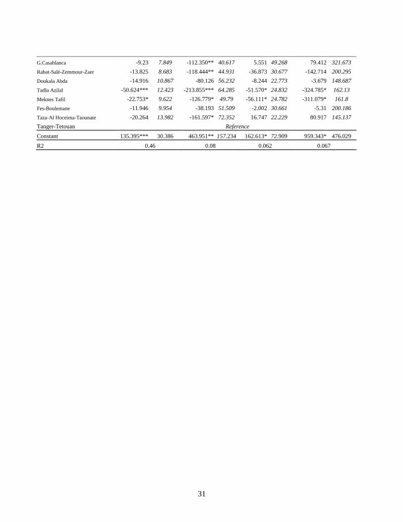
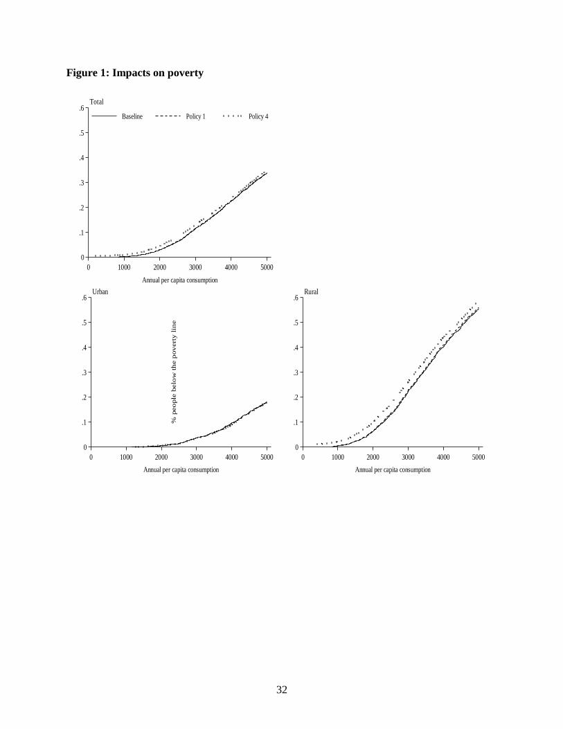
Table 3 gave our results for the impact on poverty as estimated using the government’s
official poverty lines. It is important to test robustness to alternative poverty lines. For this
purpose, we use the “poverty incidence curve,” which is simply the cumulative distribution
function up to a reasonable maximum poverty line. The results are given in Figure 1; to make
10
Notice that there is no income from meat recorded in the data. The most plausible explanation is
that Moroccan farmers sell livestock to butchers or abattoirs rather than selling meat as such. Following
conventional survey processing practices, livestock is treated as an asset, so that proceeds from the selling
of livestock is not treated as income. This is questionable. As a test, we redid our main calculations
using the survey data on the transaction in livestock, and adding net sales into income. This made
negligible difference to the results. Details are available from the authors. 11
These have been updated using the CPI. The poverty lines were 3922 Dirham per year in urban
areas and 3037 in rural areas. See World Bank (2001) for details.

11
the figure easier to read we focus on Policies 1 and 4. (The curves for Policies 2 and 3 are
between these two.)
We see that there is an increase in poverty overall from complete de-protection; this is
robust to the poverty line and poverty measure used (within a broad class of measures; see
Atkinson, 1987). The impact on poverty is almost entirely in rural areas; indeed, there is
virtually no impact on urban poverty. However, in rural areas the results in Figure 1 suggest a
sizeable impact on poverty from complete de-protection. The mean loss as a proportion of
consumption for the poorest 15% in rural areas is about 10%. There is an increase in the
proportion of the rural population living below 2000 Dirham per person per year from 6.2% to
9.9%; the proportion living below 3000 Dirham rises from 22.2% to 26.3%. (For the country as
a whole, the poverty rate for the former poverty line rises from 2.8% to 4.4% under Policy 4,
while it rises from 11.4% to 13.1% for the 3000 Dirham line.)
Our finding of adverse impacts on the rural poor contradicts claims made by some
observers who have argued that the rural poor tend to be net consumers of cereals, the
commodity that incurs the largest price decrease with this trade reform (Table 1). We will return
to this point when we study the welfare impacts further.
Table 4 gives the mean impacts of Policy 4 by region, split urban and rural. Impacts in
urban areas are small in all regions, with the highest net gain as a percentage of consumption
being 1.3% in Tanger-Tetouan, closely followed by Tensift Al Haouz and Fes-Boulemane. The
rural areas with largest mean losses from de-protection of cereals are Tasla Azilal, Meknes Tafil,
Fes-Boulemane and Tanger-Tetouan. Table 4 also gives mean impacts for the poorest 15% in
rural areas (in terms of consumption per person). When we focus on the rural poor defined this
way, the region incurring the largest mean loss for rural households is Tanger-Tetouan, followed
by Fes-Boulemane and Chaouia-Ouardigha. The contrast between the small net gains to the
urban sector and net losses to the rural poor is most marked in Tanger-Tetouan.
To begin exploring the heterogeneity in welfare impacts, Figure 2 gives the cumulative
frequency distributions of the gains and losses. To simplify the figure we again focus on Policies
1 and 4. We find that with complete de-protection (Policy 4) about 8.9% of the households
incurred losses greater than 500 Dirhams per year (about 5% of overall mean consumption)
while about 5% lose more than 1000 Dirhams per year. As one would expect, there is a “thicker
12
tail” of negative gains for rural areas. About 16% of rural households lose more that 500
Dirhams and 10% lose more than 1000.
In Figure 3 we plot the mean gains against percentiles of consumption per capita for
Policies 1 and 4. We give both absolute gains/losses and gains as a % of the household’s
consumption. For policy 1, there is a tendency for the mean absolute gain to rise as one moves
from the poorest percentile through to the richest, though the gradient is small. The mean
proportionate gain is quite flat. For Policy 4, mean absolute impacts also rise up to the richest
decile or so, but then fall. Proportionate gains follow the same pattern though (again) the
gradient seems small.
However, what is most striking from Figure 3 is the wide spread of impacts, particularly
downwards (indicating losers from the reform). The variance in absolute impacts is especially
large at the upper end of the consumption distribution, though if anything the dispersion in
proportionate impacts tends to be greater at the other end of the distribution, amongst the
poorest.
In Figure 4 we provide a split between producers and consumers for Policy 4. As we
would expect, to the extent that there is much impact on producers, they tend to lose, though not
more so for poor producers than rich ones. For consumption we tend to see more gainers, and a
higher variance in impact as one moves up the consumption distribution. However, we see that
the downward dispersion in total welfare impacts in Figure 3 is due more to the conditional
variance in impacts through production than through consumption.
There are two quite striking findings in these Figures. Firstly, notice that there are
sizeable losses on the production side amongst the poor. Granted, some large losses are evident
for the high income groups. But the claims that the poor do not lose as producers are clearly
false. Furthermore, the poor are often not seeing compensatory gains as consumers.
Secondly, it is notable that the results in Figures 3 and 4 indicate that the mean gains vary
little with mean consumption. Focusing on the “poor” versus the “rich” is hardly of much
interest in characterizing gainers and losers from this reform. The diversity in impacts tend to be
“horizontal” in the distribution of income, meaning that there tend to be larger differences in
impacts at given consumption than in mean impacts between different levels of consumption.
Next we examine these two findings in greater detail.
3.3 Who are the net producers of cereals in Morocco?

13
In the population as a whole, we find that 16% of households are net producers (value of
cereals production exceeds consumption). These households are worse off from the fall in cereal
prices due to de-protection. In rural areas, the proportion is 36%.
However, the survey data do not support the claim that the rural poor in Morocco are on
average net consumers of cereals. Figure 5 shows how producers and net producers are spread
across the distribution of total household consumption per person in rural Morocco. We give
both the scatter of points and the conditional means estimated using the local regression
method.12
In the first (top left) panel we give the proportion of producers. Then we give the
proportion of net producers (for whom production exceeds consumption of cereals in value
terms). Finally we give net production in value terms. In each case the horizontal axis gives the
percentile of the distribution of consumption from poorest through to richest.
We find that a majority of the rural poor produce cereals. Naturally much of this is for
home consumption. However, even if we focus solely on net producers, we find that over one
third of the poorest quintile tend to produce more than they consume. Furthermore, the mean net
production in value terms tends to be positive for the poor; in rural areas, the losses to poor
producers from falling cereal prices outweigh the gains to poor consumers. More than any single
feature of the survey data, it is this fact that lies at the heart of our finding that the rural poor lose
from the reform.
3.4 Vertical versus horizontal impacts on inequality
To measure the relative importance of the vertical versus horizontal differences in
impact, we can use the decomposition method outlined in section 2. This decomposition requires
an estimate of the conditional mean )( ygE , i.e., the regression function of g on y. We estimated
this using the nonparametric local regression method of Cleveland (1979).
Table 5 gives the results of this decomposition for each policy reform. For the small
partial reform under Policy 1, the vertical component dominates, accounting for 73% of the
impact on inequality. However, as one moves to the bigger reforms, the horizontal component
becomes relatively large. Indeed, we find that 119.8% of the impact of Policy 4 on inequality is
attributable to the horizontal component, while -19.8% is due to the vertical component. So we
12
See Cleveland (1979). This is often referred to as LOWESS (Locally Weighted Scatter Plot
Smoothing). We used the LOWESS program in STATA.

14
find that the vertical component was inequality reducing for Policy 4, even though overall
inequality rose (Table 5).
There is clearly a high degree of horizontal inequality in measured impacts at given mean
consumption. Some of this is undoubtedly measurement error, which may well become more
important for larger reforms. But some is attributable to observable covariates of consumption
and production behavior, as discussed in section 2. In trying to explain this variance in welfare
impacts, the characteristics we consider include region of residence, whether the household lives
in an urban area, household’s size and demographic composition, age and age-squared of the
household head, education and dummy variables describing some key aspects of the occupation
and principle sector of employment; Table 6 gives summary statistics on the variables to be used
in the regressions. We recognize that there are endogeneity concerns about these variables,
though we think those concerns are minor in this context, especially when weighed against the
concerns about omitted variable bias in estimates that exclude these characteristics. Under the
usual assumption that the error term is orthogonal to these regressors we estimate equation (6) by
Ordinary Least Squares.
The results are given in Table 7. Recall that these are averages across the impacts of
these characteristics on the consumption and production choices that determine the welfare
impact of given price and wage changes. This makes interpretation difficult. We view these
regressions as being mainly of descriptive interest, to help isolate covariates of potential
relevance in thinking about compensatory policy responses.
Focusing first on the results for Policy 4, we find that larger losses from full de-protection
of cereals are associated with families living in rural areas, that are relatively smaller (the turning
point in the U-shaped relationship is at a household size of about one), have more wage earners,
higher education, work in commerce, transport etc., and live in Chaouia-Ouardigha, Rabat, Tadla
Azilal and Meknes Tafil. Recall that these effects stem from the way household characteristics
influence net trading positions in terms of the commodities for which prices change. So, for
example, it appears that larger families tend to consume more cereals, and so gain more from the
lower cereals prices. Results are similar for partial de-protection, though education becomes
insignificant for Policy 1.
In Table 8 we give an urban-rural breakdown of the regressions for Policies 1 and 4.
There are a couple of notable differences. (Again we focus on Policy 4 in the interests of

15
brevity.) We find significant positive effects of having more children and teenagers on the gains
from trade reform in rural areas, presumably because such families are more likely to be cereal
consumers. The education effect at higher levels of schooling is much more pronounced in
urban areas. The effect of working in the transport and commerce sector is more statistically
significant in urban areas, though this effect is still sizeable in rural areas. The regional effects
are more statistically significant in urban areas than in rural areas. Of course there are still
sizable regional differences in mean impacts in Table 8, though they are statistically less
significant than we found in Table 7. In fact the quantitative magnitudes of the regional
differences are just as large for rural areas in Table 8 as for urban plus rural areas in Table 7.
It should not be forgotten that the results in Tables 7 and 8 are conditional geographic
effects (conditional on the values taken by other covariates in the regressions). As we saw in
Table 4, there are pronounced (unconditional) geographic differences in mean impacts in rural
areas across different regions. Whether one draws policy lessons more from the conditional or
unconditional effects depends on the type of policy one is using. If it is simply regional targeting
then of course the unconditional geographic effects in Table 4 will be more relevant. However,
finer targeting by household characteristics, in combination with regional targeting, will call for
the sorts of results presented in Tables 7 and 8.
The share of the variance in gains that is accountable to these covariates is generally less
than 10%. Values of R2 of this size are common in regressions run on large cross-sectional data
sets, though it remains true that a large share of the variance in impacts is not accountable to
these covariates. (The exception to our low R2
is for Policy 1, for which almost half of the
variance in gains across urban households is explained.) It must be expected that there is a
sizable degree of measurement error in the gains, stemming from measurement error in the
underlying consumption and production data. No doubt there are also important idiosyncratic
factors in household-specific tastes or production choices.
These regressions try to explain the variance in the gains from the reform. It is of interest
to see if we can do any better in explaining the incidence of losses from reform amongst the
poor. This is arguably of greater relevance to compensatory policies, which would presumably
want to focus on those amongst the poor who lose from the reforms. To test how well the same
set of regressors could explain who was a poor loser from the reforms we constructed a dummy
variable taking the value unity if a rural household incurred a negative loss and was “poor”; to

16
assure a sufficient number of observations taking the value unity we set the poverty line higher
than the official line, namely at a consumption per person of 5,000 Dirham per year (rather than
the official line of about 3,000). (We confined this to rural areas since that is where the losses
are concentrated.) In the case of full de-protection (Policy 4), we find that about 14% of the
variance in this measure can be explained by the set of regressors in Table 8 while for Policy 1
the share is 20%.13
While there are a number of covariates for identifying likely losers amongst
the poor, it is also clear that there is a large share of the variance left unexplained.
Another way to assess how effectively this set of covariates can explain the incidence of
a net loss from reform amongst the poor is by comparing the actual value of the dummy variable
described above with its predicted values from the model, using a cut off probability of 0.5. For
Policy 4, there are 472 households out of 2,100 who were both poor and incurred a loss due to
the reform. Of these the model could only correctly predict that this was the case for 18% (86
households). For Policy 1, the model prediction was correct for 27% of the 463 households who
were both poor and were made worse off by the reform.
Yet most forms of indicator targeting — whereby transfers are contingent on readily
observed variables, such as location — would be based on similar variables to those we have
used in our regressions; indeed, if anything targeted policies use fewer dimensions. This
suggests that indicator targeting will be of only limited effectiveness in reaching those in greatest
need. Self-targeting mechanisms that create incentives for people to correctly reveal their status
(such as using work requirements) may be better able to do so,
3.5 Two caveats
While the above results are suggestive, two limitations of our analysis should be noted.
The first stems from the fact that the Doukkali (2003) model assumed fixed wage rates. While
sensitivity to alternative labor market assumptions should be checked, we can speculate on the
likely impacts of allowing real wages to adjust to the reforms. Here it can be argued that the
export-oriented cash crops that will replace cereals will tend to be more labor intensive than
cereals. Thus we would expect higher aggregate demand for the relatively unskilled labor used
in agriculture, and hence higher real wages for relatively poorer groups. This will undoubtedly
13
The R2 for OLS regressions are 0.139 and 0.191 for Policy 4 and 1 respectively. Using instead a
probit model to correct for the nonlinearity the pseudo R2’s are 0.135 and 0.196.

17
go some way toward compensating the rural poor, and may even tilt the vertical distributional
impacts in favor of the poor.
A second concern is that there may well be dynamic gains from greater trade openness
that are not being captured by the model used to generate the relative price impacts; for example,
trade may well facilitate learning about new agricultural technologies and innovation that brings
longer-term gains in farm productivity. These effects may be revealed better by studying time
series evidence, combined with cross-country comparisons.
4. Conclusions
The welfare impacts of de-protection in developing countries have been much debated.
Some people have argued that external trade liberalizations are beneficial to the poor while
others argue that the benefits will be captured more by the non-poor. Expected impacts on
domestic prices have figured prominently in these debates.
The paper has studied the welfare impacts at household level of the changes in
commodity prices attributed to a proposed trade reform, namely Morocco’s de-protection of its
cereals sector. This would entail a sharp reduction in tariffs, with implications for the domestic
structure of prices and hence household welfare. The paper draws out the implications for
household welfare of the previous estimates of the price impacts of reform done for a Joint
Government of Morocco and World Bank Committee. The estimates of price impacts are
entirely external to (and pre-date) our analysis. All we do here is to use some standard methods
of first-order welfare analysis to measure the gains and losses at household level using a large
sample survey. In future work using this methodology, there may well be more scope for
feedbacks from the household-level analysis to the CGE modeling used to derive price impacts.
In a number of respects, our detailed household-level analysis throws into question past
claims about the likely welfare impacts of this trade reform. In the aggregate, we find a small
negative impact on mean household consumption and a small increase in inequality. There is a
sizable, and at least partly explicable, variance in impacts across households. Rural families tend
to lose; urban households tend to gain. There are larger impacts in some provinces than others,
with highest negative impacts for rural households in Tasla Azilal, Meknes Tafil, Fes-Boulemane
and Tanger-Tetouan. Mean impacts for rural households in these regions are over 10% or more

18
of consumption. There are clearly sizeable welfare losses amongst the poor in these specific
regions.
The adverse impact on rural poverty stems in large part from the fact that the losses to the
net producers of cereals outweigh the gains to the net consumers amongst the poor. Thus, on
balance rural poverty rises. This contradicts the generalizations that have been made in the past
that the rural poor in Morocco tend to be net consumers of grain, and hence gainers from trade
reform. Yes, a majority are net consumers, but on balance the welfare impacts on the rural poor
are negative.
Our results lead us to question the high level of aggregation common in past claims about
welfare impacts of trade reform. We find diverse impacts at given pre-reform consumption
levels. This “horizontal” dispersion becomes more marked as the extent of reform (measured by
the size of the tariff cut) increases. Indeed, we estimate that all of the impact of complete de-
protection of cereals on inequality is horizontal rather than vertical; the vertical impact on
inequality was actually inequality reducing. For a modest reform of a 10% cut in tariffs, the
vertical component dominates, though there is still a large horizontal component. It is clear from
our results that in understanding the social impacts of this reform, one should not look solely at
income poverty and income inequality as conventionally measured; rather one needs to look at
impacts along “horizontal” dimensions, at given income.
We have been able to identify some specific types of households whose consumption and
production behavior makes them particularly vulnerable. These results are suggestive of the
targeting priorities for compensatory programs. The fact that we also find a large share of
unexplained variance in impacts also points to the limitations of targeting based on readily
observable indicators, suggesting that self-targeting mechanisms may also be needed.

19
Appendix: Measuring welfare impacts at the household level
The approach used here is reasonably standard, but it is still worth spelling out the
specifics to see more clearly how the analysis in this paper is done.
Each household is assumed to have preferences over consumption and work effort
represented by the utility function ),( idii Lqu
where d
iq is a vector of the quantities of
commodities demanded by household i and iL is a vector of labor supplies by activity, including
supply to the household’s own production activities.14
The household is assumed to be free to
choose its preferred combinations of diq and iL subject to its budget constraint. The production
activity owned by the household generates a profit )](max[)( sii
si
si
sii qcqpp
where s
ip is a
vector of supply prices, and )( sii qc is the household-specific cost function.
15 The indirect utility
function of household i is given by:
])(),([max],,[),(
siiii
di
dii
dii
Lqi
di
sii pLwqpLquwppv
idi
(A1)
where dip is the price vector for consumption, iw is the vector of wage rates.
Taking the differential of (1) and using the envelope property (whereby the welfare
impacts in a neighborhood of an optimum can be evaluated by treating the quantity choices as
given), the gain to household i (denoted ig ) is given by the money metric of the change in
utility:
n
k k
ksikk
m
jdij
dijd
ijdijs
ij
sijs
ijsij
i
ii
w
dwLw
p
dpqp
p
dpqp
v
dug
11
)(][
(A2)
where iv is the marginal utility of income for household i (the multiplier on the budget
constraint in equation A1) and sikL is the household’s “external” labor supply to activity k.
(Notice that gains in earnings from labor used in own production are exactly matched by the
higher cost of this input to own-production.) The proportionate changes in prices are weighted
by their corresponding expenditure shares; the weight for the proportionate change in the j’th
14
We make the standard assumptions that goods have positive marginal utilities while labor
supplies have negative marginal utilities. 15
On can readily include input prices in this cost function; see Chen and Ravallion (2004) for a
more general formulation. In the present context this makes no difference to the subsequent analysis so
we subsume factor prices in the cost function to simplify notation.

20
selling price is sij
sijqp , the revenue (selling value) from household production activities in sector j;
similarly dij
dij qp is the (negative) weight for demand price changes and s
ikk Lw is the weight for
changes in the wage rate for activity k. The term dij
dij
sij
sij qpqp gives (to a first-order
approximation) the welfare impact of an equi-proportionate increase in the price of commodity j.
Equation (A2) is the key formula we will use for calculating the welfare impacts at household
level, given the predicted price changes.
Having estimated the impacts at household level, we can study how they vary with pre-
reform welfare, and what impact the reform has on poverty and inequality. We can also try to
explain the differences in impacts in terms of observable characteristics of potential relevance to
social protection policies. The way we have formulated the problem of measuring welfare
impacts above allows utility and profit functions to vary between households at given prices. To
try to explain the heterogeneity in measured welfare impacts we can suppose instead that these
functions vary with observed household characteristics. The indirect utility function becomes:
]),,(max[),,,,(),,( 121 iiidi
diii
diiii
di
sii
di
sii LwqpxLquxxwppvwppv (A3)
where
)],(max[),( 22 isi
si
sii
sii xqcqpxp (A4)
Note that we allow the characteristics that influence preferences over consumption ( ix1 ) to differ
from those that influence the profits from own-production activities ( ix2 ). The gain from the
price changes induced by trade reform, as given by equation (A3), depends on the consumption,
labor supply and production choices of the household, which depend in turn on prices and
characteristics, ix1 and ix2 . Generically, we can now write the gain as equation (5).

Table 1: Predicted price changes due to agricultural trade reform in Morocco
Sectors Consumers (% change in prices) Producers (% change in prices)
Policy 1 Policy 2 Policy 3 Policy 4 Policy 1 Policy 2 Policy 3 Policy 4
Cereals and cereals products -3.062 -7.786 -12.811 -26.691 -2.858 -7.193 -11.744 -24.107
Fresh vegetables -0.714 -0.884 -1.051 -1.128 -0.580 -0.767 -0.871 -0.756
Fruits -0.637 -0.681 -0.683 -0.139 -0.429 -0.301 -0.104 0.843
Dairy products and eggs -0.472 -0.414 -0.257 0.751 -0.505 -0.487 -0.333 0.637
Meat (red and poultry) -0.320 -0.109 0.332 1.896 -0.306 -0.078 0.357 1.936
Sugar -0.200 0.100 0.400 1.300 -0.368 -0.378 -0.354 -0.094
Edible oils -0.671 -1.064 -1.405 -2.225 -0.632 -0.998 -1.336 -2.061
Fresh and processed fish 0.000 0.696 1.300 2.996 0.000 0.600 1.300 2.881
Other ag. and processed food -0.369 -0.402 -0.421 -0.635 0.268 1.294 2.475 5.388
Services 0.142 0.500 0.758 1.460 0.056 0.500 0.844 1.708
Energy, electricity and water -0.060 0.540 1.140 2.580 -0.051 0.549 1.149 2.597
Other industries 0.000 0.600 1.200 2.800 0.000 0.600 1.200 2.793
Note: The tariff cuts on imported cereals are 10%, 30%, 50% and 100% for Policies 1,2,3 and 4 respectively.

22
Table 2a: Consumption shares and welfare impacts through consumption
Consumption
Shares
Policy 1
Policy 2
Policy 2
Policy 4
National
Cereals 0.084 0.257 0.654 1.076 2.242
Fresh vegetables 0.042 0.030 0.037 0.044 0.047
Fruits 0.022 0.014 0.015 0.015 0.003
Dairy products and eggs 0.032 0.015 0.013 0.008 -0.024
Meat (red and poultry) 0.112 0.036 0.012 -0.037 -0.213
Sugar 0.015 0.003 -0.002 -0.006 -0.019
Edible oils 0.032 0.021 0.034 0.044 0.070
Fresh and processed fish 0.013 0.000 -0.009 -0.017 -0.038
Ag. and processed food 0.101 0.037 0.040 0.042 0.064
Services 0.066 -0.009 -0.033 -0.050 -0.097
Energy, electricity, water 0.148 0.009 -0.080 -0.169 -0.382
Other industries 0.333 0.000 -0.200 -0.400 -0.933
Total 1.000 0.413 0.482 0.551 0.719
Urban
Cereals 0.066 0.203 0.517 0.851 1.773
Fresh vegetables 0.037 0.026 0.033 0.0390 0.042
Fruits 0.022 0.014 0.015 0.015 0.003
Dairy products and eggs 0.034 0.016 0.014 0.009 -0.026
Meat (red and poultry) 0.107 0.034 0.012 -0.035 -0.203
Sugar 0.011 0.002 -0.001 -0.004 -0.014
Edible oils 0.024 0.016 0.026 0.034 0.054
Fresh and processed fish 0.014 0.000 -0.010 -0.018 -0.041
Ag. and processed food 0.096 0.035 0.039 0.040 0.061
Services 0.067 -0.010 -0.033 -0.051 -0.097
Energy, electricity, water 0.155 0.009 -0.084 -0.176 -0.399
Other industries 0.368 0.000 -0.221 -0.441 -1.030
Total 1.000 0.348 0.307 0.262 0.123
Rural
Cereals 0.136 0.415 1.056 1.738 3.622
Fresh vegetables 0.055 0.039 0.049 0.058 0.062
Fruits 0.021 0.014 0.015 0.015 0.003
Dairy products and eggs 0.028 0.013 0.011 0.007 -0.021
Meat (red and poultry) 0.128 0.041 0.014 -0.043 -0.243
Sugar 0.028 0.006 -0.003 -0.011 -0.036
Edible oils 0.053 0.036 0.056 0.075 0.118
Fresh and processed fish 0.010 0.000 -0.007 -0.013 -0.029
Ag. and processed food 0.115 0.042 0.046 0.048 0.073
Services 0.066 -0.009 -0.033 -0.050 -0.097
Energy, electricity, water 0.129 0.008 -0.070 -0.147 -0.332
Other industries 0.232 0.000 -0.139 -0.278 -0.650
Total 1.000 0.604 0.996 1.399 2.471

23
Table 2b: Percentage gains from each policy: Production component
Production
as a share of
total consumption
Policy 1
Policy 2
Policy 2
Policy 4
National
Cereals 0.089 -0.271 -0.690 -1.135 -2.365
Fresh vegetables 0.053 -0.038 -0.047 -0.056 -0.060
Fruits 0.041 -0.026 -0.028 -0.028 -0.006
Dairy products and eggs 0.051 -0.024 -0.021 -0.013 0.039
Meat (red and poultry) 0.000 0.000 0.000 0.000 0.000
Sugar 0.000 0.000 0.000 0.000 0.000
Edible oils 0.025 -0.017 -0.027 -0.035 -0.056
Fresh and processed fish 0.000 0.000 0.000 0.000 0.000
Ag. and processed food 0.002 -0.001 -0.001 -0.001 -0.001
Services 0.000 0.000 0.000 0.000 0.000
Energy, electricity, water 0.000 0.000 0.000 0.000 0.000
Other industries 0.000 0.000 0.000 0.000 0.000
Total 0.262 -0.377 -0.814 -1.269 -2.450
Urban
Cereals 0.010 -0.031 -0.079 -0.130 -0.272
Fresh vegetables 0.008 -0.006 -0.007 -0.009 -0.009
Fruits 0.016 -0.011 -0.011 -0.011 -0.002
Dairy products and eggs 0.007 -0.003 -0.003 -0.002 0.005
Meat (red and poultry) 0.000 0.000 0.000 0.000 0.000
Sugar 0.000 0.000 0.000 0.000 0.000
Edible oils 0.013 -0.009 -0.014 -0.018 -0.029
Fresh and processed fish 0.000 0.000 0.000 0.000 0.000
Ag. and processed food 0.000 0.000 0.000 0.000 0.000
Services 0.000 0.000 0.000 0.000 0.000
Energy, electricity, water 0.000 0.000 0.000 0.000 0.000
Other industries 0.000 0.000 0.000 0.000 0.000
Total 0.054 -0.059 -0.114 -0.170 -0.307
Rural
Cereals 0.319 -0.978 -2.487 -4.091 -8.524
Fresh vegetables 0.186 -0.133 -0.165 -0.195 -0.210
Fruits 0.113 -0.072 -0.077 -0.077 -0.016
Dairy products and eggs 0.183 -0.086 -0.076 -0.047 0.138
Meat (red and poultry) 0.000 0.000 0.000 0.000 0.000
Sugar 0.000 0.000 0.000 0.000 0.000
Edible oils 0.061 -0.041 -0.065 -0.086 -0.136
Fresh and processed fish 0.000 0.000 0.000 0.000 0.000
Ag. and processed food 0.008 -0.003 -0.003 -0.004 -0.005
Services 0.000 0.000 0.000 0.000 0.000
Energy, electricity, water 0.000 0.000 0.000 0.000 0.000
Other industries 0.000 0.000 0.000 0.000 0.000
Total 0.870 -1.313 -2.872 -4.500 -8.753

24
Table 3: Household impacts of four trade reforms
Baseline Policy 1 Policy 2 Policy 3 Policy 4
National
Poverty rate (%) 19.61 20.01 20.33 21.04 22.13
Mean Log Deviation (x100) 28.50 28.92 29.00 29.14 29.17
Gini index (x100) 38.50 38.70 38.90 39.10 39.50
Per capita gain 0 6.52 -23.97 -54.82 -133.81
Mean % gain: price changes
weighted by mean shares 0 -0.059 -0.513 -0.971 -2.141
Mean % gain: weighted by
ratios of means (Tables 2a,b) 0 0.035 -0.332 -0.718 -1.731
Production gain 0 -32.08 -69.01 -106.31 -201.02
Consumption gain 0 38.60 45.05 51.49 67.21
Consumption per capita 9350.91 9357.43 9326.95 9296.10 9217.10
Urban
Poverty rate (%) 12.19 12.05 11.96 12.05 11.76
Mean Log Deviation (x100) 25.49 25.41 25.32 25.23 24.93
Gini index (x100) 36.60 36.50 36.50 36.40 36.20
Per capita gain 0 35.52 24.80 13.75 -16.49
Mean % gain: price changes
weighted by mean shares 0 0.36 0.37 0.39 0.44
Mean % gain: weighted by
ratios of means (Tables 2a,b) 0 0.29 0.193 0.092 -0.184
Production gain 0 -6.31 -12.10 -17.79 -31.30
Consumption gain 0 41.83 36.90 31.54 14.81
Consumption per capita 12031.20 12066.72 12056 12044.95 12014.71
Rural
Poverty rate (%) 28.28 29.31 30.10 31.54 34.25
Mean Log Deviation (x100) 17.47 17.82 17.82 17.93 17.76
Gini index (x100) 31.20 31.30 31.50 31.80 32.80
Per capita gain 0 -33.53 -91.32 -149.51 -295.85
Mean % gain: price changes
weighted by mean shares 0 -0.63 -1.74 -2.85 -5.71
Mean % gain: weighted by
ratios of means (Tables 2a,b) 0 -0.71 -1.88 -3.10 -6.28
Production gain 0 -67.67 -147.61 -228.56 -435.42
Consumption gain 0 34.14 56.29 79.05 139.57
Consumption per capita 5649.03 5615.50 5557.71 5499.52 5353.19
Note: All monetary units are Moroccan Dirham per year. MLD is only calculated over the set of households for
whom consumption is positive. The mean % gains weighted by mean shares are simply the means across the sample
of the % gains at household level. The second mean % gain is weighted by shares at the means points based on
Tables 2a,b.

25
Table 4: Mean gains from Policy 4 by region
Region Total Urban Rural Poorest 15% of
rural households
Oued Ed-Dahab-Lagouira -0.20 -0.20 . .
Laayoune-Boujdour-Sakia El Hamra -0.34 -0.34 . .
Guelmime Es-Semara -0.96 0.72 -3.47 -0.58
Souss-Massa-Daraa -1.31 0.42 -2.4 -3.09
Gharb-Chrarda-Beni Hssen -2.16 0.02 -3.86 0.10
Chaouia-Ouardigha -4.18 0.32 -8.31 -10.11
Tensift Al Haouz -0.87 1.12 -2.17 0.31
Oriental -0.87 0.38 -2.78 0.25
G.Casablanca 0.48 0.41 2.41 .
Rabat-Salé-Zemmour-Zaer -0.59 0.33 -4.98 0.23
Doukala Abda -3.13 0.76 -5.92 -3.93
Tadla Azilal -6.93 -0.71 -11.04 -0.95
Meknes Tafil -4.89 -0.19 -11.35 -8.48
Fes-Boulemane -2.4 1.05 -11.52 -13.43
Taza-Al Hoceima-Taounate -4.47 -0.32 -5.78 -8.39
Tanger-Tetouan -2.94 1.31 -9.4 -22.03
Total -2.14 0.45 -5.71 -10.39
Note: Means formed over the household level % gains (equivalent to weighting proportionate
price changes by mean shares).
Table 5: Decomposition of the impact on inequality
Policy 1 Policy 2 Policy 3 Policy 4
Vertical component 72.69 57.57 38.77 -19.77
Horizontal component 27.31 42.43 61.23 119.77
Total 100.00 100.00 100.00 100.00
Note: The decomposition is only implemented on the sample of households for whom both the baseline
and post-reform consumption is positive.

26
Table 6: Summary statistics on explanatory variables in the regression analysis
Mean Std. Dev
Urban 0.580 binary
Log household size 1.645 0.550
Log household size 2 3.009 1.621
Female headed household 0.170 binary
If unemployed present 0.248 binary
Number of wage earners 5.912 2.878
Share of children 0-6 0.140 0.162
Share of children 7-17 0.221 0.204
Share of elderly 60+ 0.120 binary
Characteristics of the head
Age of the head 0.505 0.143
Age of the head 2 0.275 0.155
Illiterate head 0.582 binary
Incomplete primary school 0.100 binary
Primary school completed 0.164 binary
Low secondary school 0.058 binary
Upper secondary school 0.059 binary
University 0.036 binary
Industry
Not-employed 0.240 binary
Industrie/B.T.P 0.004 binary
Commerce/Transp./Commun./Admin. 0.273 binary
Service Soci. 0.085 binary
Autres services 0.064 binary
Corps Exter. 0.125 binary
Chomeur 0.012 binary
Femme au foyeur/Eleve/Etudiant 0.037 binary
Jeune enfant 0.009 binary
Vielliard/Retraite/Rentiers 0.074 binary
Infirme/malade 0.068 binary
Autre inactifs 0.010 binary
Regions
Oued Ed-Dahab-Lagouira 0.012 binary
Laayoune-Boujdour-Sakia El Hamra 0.014 binary
Guelmime Es-Semara 0.023 binary
Souss-Massa-Daraa 0.094 binary
Gharb-Chrarda-Beni Hssen 0.058 binary
Chaouia-Ouardigha 0.054 binary
Tensift Al Haouz 0.100 binary
Oriental 0.065 binary
G.Casablanca 0.124 Binary
Rabat-Salé-Zemmour-Zaer 0.081 Binary
Doukala Abda 0.067 Binary
Tadla Azilal 0.047 Binary

27
Meknes Tafil 0.072 binary
Fes-Boulemane 0.051 binary
Taza-Al Hoceima-Taounate 0.058 binary

28
Table 7: Regression of per capita gain/loss on selected household characteristics
Policy 1 Policy 2 Policy 3 Policy 4
Coeff. s.e. Coeff. s.e. Coeff. s.e. Coeff. s.e.
Urban 26.139*** 6.275 44.850*** 12.948 64.218** 20.068 113.714** 39.213
Log household size -57.242** 19.583 -78.454* 40.407 -100.548 62.626 -157.373 122.376
Log household size 2 77.337*** 16.806 167.523*** 34.678 260.865*** 53.746 508.026*** 105.023
Female headed household 2.502 7.431 4.072 15.333 5.605 23.765 9.161 46.438
If unemployed present 10.018* 5.909 23.344* 12.192 36.428* 18.896 67.997* 36.924
Number of wage earners -44.722*** 7.019 -101.428*** 14.484 -159.842*** 22.448 -313.541*** 43.865
Share of children 0-6 32.783* 17.72 89.774* 36.564 145.705* 56.67 277.637* 110.736
Share of children 7-17 25.070* 14.155 69.367* 29.206 113.738* 45.266 221.518* 88.453
Share of elderly 60+ -21.3 15.584 -23.551 32.155 -24.389 49.837 -24.334 97.385
Characteristics of the head
Age of the head -38.511 108.759 -151.473 224.41 -272.681 347.809 -624.596 679.642
Age of the head 2 44.097 102.579 142.598 211.658 246.231 328.045 543.07 641.022
Household is literate
only -8.871 7.983 -23.441 16.472 -38.257 25.53 -76.735 49.888
Incomplete primary
education Reference
Primary school completed -14.013* 6.757 -40.623** 13.942 -68.220** 21.608 -141.296*** 42.224
Low secondary school -12.98 10.4 -61.634** 21.458 -112.583*** 33.258 -250.335*** 64.989
Upper secondary school -12.462 10.775 -70.619** 22.233 -130.320*** 34.458 -286.333*** 67.333
University 2.575 13.527 -95.376*** 27.912 -197.887*** 43.26 -476.077*** 84.533
Industry
Not-working/Agriculture Reference
Industrie/B.T.P -3.71 36.465 -0.277 75.242 4.541 116.616 21.281 227.874
Commerce/Transport/
Communications/Admin. -59.926*** 8.198 -122.454*** 16.915 -185.113*** 26.216 -341.751*** 51.228
Service Soci. 4.424 10.036 17.18 20.707 30.536 32.094 66.804 62.714
Autres services -0.2 11.251 9.572 23.214 19.812 35.98 47.874 70.306
Corps Exter. 2.385 8.936 6.785 18.439 10.912 28.579 20.23 55.844
Chomeur 6.627 21.518 27.715 44.399 49.65 68.813 107.951 134.465
Femme au
foyeur/Eleve/Etudiant 2.26 13.49 13.788 27.835 25.401 43.141 55.785 84.301
Jeune enfant 7.629 24.5 -3.891 50.553 -16.336 78.352 -51.207 153.104
Vielliard/Retraite/Rentiers 6.913 11.039 23.527 22.778 40.651 35.303 86.8 68.984
Infirme/malade 3.143 10.96 22.092 22.614 42.489 35.049 100.065 68.488
Autre inactifs -9.955 22.723 1.817 46.885 15.364 72.667 56.497 141.995
Regions
Oued Ed-Dahab-Lagouira 19.216 22.51 -6.738 46.446 -34.818 71.986 -111.388 140.665
Laayoune-Boujdour-Sakia
El Hamra -1.502 21.067 -20.145 43.47 -40.764 67.374 -98.323 131.652
Guelmime Es-Semara 9.666 16.639 11.901 34.333 12.774 53.212 12.391 103.979
Souss-Massa-Daraa -7.645 10.868 5.611 22.425 22.766 34.756 85.2 67.916
Gharb-Chrarda-Beni
Hssen -10.087 12.229 -7.485 25.232 -3.592 39.107 10.494 76.418
Chaouia-Ouardigha -19.542 12.507 -49.255* 25.807 -81.319* 39.998 -169.114* 78.159
Tensift Al Haouz 2.964 10.696 14.527 22.071 27.258 34.207 65.274 66.842

29
Oriental -14.038 11.928 -19.198 24.612 -23.918 38.145 -31.056 74.539
G.Casablanca -3.322 10.429 -15.762 21.518 -28.418 33.35 -60.086 65.169
Rabat-Salé-Zemmour-
Zaer -15.439 11.326 -33.817 23.371 -52.199 36.222 -97.061 70.78
Doukala Abda -13.169 11.76 -23.668 24.265 -34.315 37.607 -59.462 73.487
Tadla Azilal -55.774*** 13.093 -114.700*** 27.016 -174.099*** 41.872 -320.810*** 81.821
Meknes Tafil -37.594** 11.54 -74.192** 23.812 -111.929** 36.906 -209.391** 72.117
Fes-Boulemane -10.249 12.726 -15.356 26.259 -20.651 40.699 -33.326 79.528
Taza-Al Hoceima-
Taounate 5.613 12.367 2.43 25.517 -2.415 39.549 -21.329 77.281
Tanger-Tetouan Reference
Constant 144.096*** 34.638 247.104*** 71.472 354.469** 110.773 642.381** 216.458
R2 0.175 0.080 0.062 0.057

30
Table 8: Urban-rural split of regressions for per capita gains
Urban Rural
Policy 1 Policy 4 Policy 1 Policy 4
Coeff. s.e.
Coeff. s.e.
Coeff. s.e. Coeff. s.e.
Log household size -32.840* 16.071 45.705 83.159 -89.255* 45.084 -527.017* 294.353
Log household size 2 40.492* 17.841 217.663* 92.32 79.415* 32.524 555.880** 212.348
Female headed household -2.696 6.018 -15.603 31.139 11.984 16.902 27.785 110.356
If unemployed present 2.138 4.668 25.238 24.154 11.086 14.482 35.299 94.551
Number of wage earners -23.972** 8.39 -143.745*** 43.414 -45.101*** 12.237 -321.182*** 79.894
Share of children 0-6 -15.648 15.206 25.903 78.686 95.815** 36.544 609.370* 238.601
Share of children 7-17 -10.44 11.986 -34.073 62.023 81.378** 29.771 622.563** 194.376
Share of elderly 60+ -17.696 13.328 4.67 68.967 -35.448 32.512 -167.42 212.274
Characteristics of the head
Age of the head -26.02 96.18 -513.051 497.696 -82.081 216.7 -1.00E+03 1414.846
Age of the head 2 33.769 91.377 263.429 472.842 103.772 202.766 1129.226 1323.868
Household is literate only -10.567 6.965 -90.700* 36.042 -8.718 16.11 -75.293 105.182
Incomplete primary education Reference
Primary school completed 0.157 5.566 -44.272 28.804 -31.613* 14.794 -270.881** 96.589
Low secondary school 6.416 7.632 -119.177** 39.494 -73.971* 31.399 -655.218** 205.005
Upper secondary school -5.731 7.551 -249.358*** 39.074 10.925 49.861 -46.655 325.547
University 9.241 9.282 -433.456*** 48.03 20.185 83.244 18.883 543.507
Industry
Not-working/Agriculture Reference
Industrie/B.T.P -4.779 25.641 7.254 132.684 56.769 124.939 366.598 815.737
Commerce/Transp./Commun./
Admin. -96.116*** 10.172 -444.047*** 52.634 -43.789** 15.445 -257.349* 100.843
Service Soci. -1.428 7.574 6.102 39.191 27.61 28.965 247.156 189.116
Autres services -4.7 9.133 6.023 47.259 21.228 25.434 161.257 166.061
Corps Exter. -2.611 6.884 -19.401 35.621 8.742 23.042 57.723 150.44
Chomeur -1.702 15.213 36.377 78.72 60.148 73.543 457.084 480.167
Femme au oyeur/Eleve/Etudiant -4.019 10.145 12.554 52.498 20.295 36.207 110.127 236.4
Jeune enfant -2.268 16.343 -129.322 84.567 107.247 152.23 720.704 993.92
Vielliard/Retraite/Rentiers 1.108 8.138 48.765 42.112 25.588 34.261 154.32 223.691
Infirme/malade 1.847 8.176 63.019 42.308 5.864 30.489 148.543 199.063
Autre inactifs -12.094 16.532 23.685 85.547 22.652 67.323 250.306 439.559
Regions
Oued Ed-Dahab-Lagouira 21.2 15.068 -135.288* 77.973
Laayoune-Boujdour-Sakia El
Hamra -2.496 14.153 -129.348* 73.236
Guelmime Es-Semara 7.558 13.813 -50.41 71.475 23.284 35.563 165.753 232.195
Souss-Massa-Daraa -1.425 10.023 -54.723 51.863 -8.417 21.371 211.302 139.535
Gharb-Chrarda-Beni Hssen -44.733*** 11.143 -204.020*** 57.663 17.31 23.762 208.808 155.141
Chaouia-Ouardigha -15.625 11.08 -89.734 57.333 -19.527 25.012 -201.804 163.304
Tensift Al Haouz -8.763 9.759 -37.2 50.5 8.732 21.097 147.015 137.74
Oriental -18.776* 9.806 -96.129* 50.74 -0.357 25.851 99.206 168.782
31
G.Casablanca -9.23 7.849 -112.350** 40.617 5.551 49.268 79.412 321.673
Rabat-Salé-Zemmour-Zaer -13.825 8.683 -118.444** 44.931 -36.873 30.677 -142.714 200.295
Doukala Abda -14.916 10.867 -80.126 56.232 -8.244 22.773 -3.679 148.687
Tadla Azilal -50.624*** 12.423 -213.855*** 64.285 -51.570* 24.832 -324.785* 162.13
Meknes Tafil -22.753* 9.622 -126.779* 49.79 -56.111* 24.782 -311.079* 161.8
Fes-Boulemane -11.946 9.954 -38.193 51.509 -2.002 30.661 -5.31 200.186
Taza-Al Hoceima-Taounate -20.264 13.982 -161.597* 72.352 16.747 22.229 80.917 145.137
Tanger-Tetouan Reference
Constant 135.395*** 30.386 463.951** 157.234 162.613* 72.909 959.343* 476.029
R2 0.46 0.08 0.062 0.067
32
Figure 1: Impacts on poverty
0
.1
.2
.3
.4
.5
.6
% p
eo
ple
belo
w t
he p
ov
ert
y l
ine
0 1000 2000 3000 4000 5000
Annual per capita consumption
Baseline Policy 1 Policy 4
Total
0
.1
.2
.3
.4
.5
.6
% p
eo
ple
belo
w t
he p
ov
ert
y l
ine
0 1000 2000 3000 4000 5000
Annual per capita consumption
Urban
0
.1
.2
.3
.4
.5
.6
% p
eo
ple
belo
w t
he p
ov
ert
y l
ine
0 1000 2000 3000 4000 5000
Annual per capita consumption
Rural

Figure 2: Frequency distributions of gains/losses for Policies 1 and 4
0
.1
.2
.3
.4
.5
.6
.7
.8
.9
1
Cum
ula
tiv
e d
ensit
y
-3000 -2000 -1000 0 1000-500 500
Total
0
.005
.01
.015
.02
Pro
babil
ity
densit
y
-600 -400 -200 0 200 400
Policy 1
Policy 4
Total
0
.1
.2
.3
.4
.5
.6
.7
.8
.9
1
Cum
ula
tiv
e d
ensit
y
-3000 -2000 -1000 0 1000-500 500
Absolute gain pre capita
Urban
0
.1
.2
.3
.4
.5
.6
.7
.8
.9
1
Cum
ula
tiv
e d
ensit
y
-3000 -2000 -1000 0 1000-500 500
Absolute gain per capita
Rural

34
Figure 3: Absolute and proportionate gains for Policies 1 and 4 plotted against percentile of
consumption
-3000
-2500
-2000
-1500
-1000
-500
0
500
1000
1500
abso
lute
gai
n/l
oss
per
cap
ita
0 10 20 30 40 50 60 70 80 90 100
Policy 1
-3000
-2500
-2000
-1500
-1000
-500
0
500
1000
1500
0 10 20 30 40 50 60 70 80 90 100
Policy 4
-50
-35
-20
-5
10
25
0
5
% g
ain/l
oss
per
cap
ita
0 10 20 30 40 50 60 70 80 90 100
Per capita consumption percentiles
-50
-35
-20
-5
10
25
0
5
0 10 20 30 40 50 60 70 80 90 100
Per capita consumption percentiles

35
Figure 4: Production/consumption decomposition of the welfare impacts for Policy 4,
plotted against percentile of consumption per person
-3000
-2500
-2000
-1500
-1000
-500
0
500
1000
1500
absolu
te g
ain
/loss
per
capit
a
0 10 20 30 40 50 60 70 80 90 100
Per capita consumption percentiles
Policy 4, production
-3000
-2500
-2000
-1500
-1000
-500
0
500
1000
1500
0 10 20 30 40 50 60 70 80 90 100
Per capita consumption percentiles
Policy 4, consumption

36
Figure 5: Net producers of cereals in the distribution of total consumption per person in
rural areas
0
.25
.5
.75
1
% c
ereal
pro
du
cers
0 10 20 30 40 50 60 70 80 90 100
0
.25
.5
.75
1
% n
et
pro
du
cer
s o
f ce
reals
0 10 20 30 40 50 60 70 80 90 100
Consumption per capita percentiles
-.5
-.25
0
.25
.5
.75
1
Pro
du
ctio
n m
inu
s co
nsu
mp
tio
n o
f cer
eal
s
as
a p
rop
ort
ion
of
tota
l co
nsu
mp
tio
n
0 10 20 30 40 50 60 70 80 90 100
Consumption per capita percentiles

37
References
Abdelkhalek, Touhami, 2002, “De I’impact de la Libéralization du Marche Céréalier Marocain:
Enseignements à Partir d’un Modèle de Comportement des Ménages Rureaux, Critique
Economique 7 : 105-114.
Atkinson, Anthony B., 1987, “On the Measurement of Poverty,” Econometrica 55: 749-764.
Auerbach, Alan J., and Kevin A. Hassett, 2002, “A New Measure of Horizontal Equity,”
American Economic Review 92(4): 1116-1125.
Bourguignon, Francois, 1979, “Decomposable Inequality Measures,” Econometrica, 47: 901-
920.
Bourguignon in Francois and Luiz Pereira Da Silva (eds), 2003, The Impact of Economic
Policies on Poverty and Income Distribution: Evaluation Techniques and Tools. New
York: Oxford University Press.
Chen, Shaohua and Martin Ravallion, 2004, “Welfare Impacts of Morocco’s Accession to the
WTO,” World Bank Economic Review, 18(1): 29-58.
Cleveland, William S., 1979, “Robust Locally Weighted Regression and Smoothing Scatter
Plots,” Journal of the American Statistical Association 74: 829-36.
Cockburn, John. 2002. “Trade Liberalization and Poverty in Nepal: A Computable General
Equilibrium Micro Simulation Analysis.” University of Laval.
Cowell, Frank, 2000, “Measurement of Inequality,” in A.B. Atkinson and F. Bourguignon
(eds) Handbook of Income Distribution, Amsterdam: North-Holland.
Doukkali, Rachid, 2003, “Etude de Effets de la Libéralisation des Céréales: Resultats des
Simulaions à L’Aide d’un Modèle Equilibre Général Calculable,” Joint Report of the
Ministry of Agriculture and the World Bank.
Hertel, Thomas W. and Jeffrey Reimer, 2004, “Predicting the Poverty Impacts of Trade

38
Liberalization: A Survey,” Department of Agricultural Economics, Purdue University.
McCulloch, Neil, L. Alan Winters, and Xavier Cirera. 2001. Trade Liberalization and Poverty: A
Handbook. London: Center for Economic Policy Research and Department for
International Development.
Ravallion, Martin, 2001, “Growth, Inequality and Poverty: Looking Beyond Averages,”
World Development, 29(11), 1803-1815.
______________, 2004, “Competing Concepts of Inequality in the Globalization Debate,”
Policy Research Working Paper, World Bank, Washington DC.
Ravallion, Martin and Dominique van de Walle, 1991, “The Impact of Food Pricing
Reforms on Poverty: A Demand Consistent Welfare Analysis for Indonesia,”
Journal of Policy Modeling, 13: 281-300.
World Bank, 2001, Kingdom of Morocco: Poverty Update. Washington DC, World Bank.
__________, 2003, Kingdom of Morocco: Findings and Recommendations of the
Cereals Working Group: A Critical Review, Washington DC, World Bank.