Chinese Journal of Aeronautics, (2016), 29(5): 1262–1272

Chinese Society of Aeronautics and Astronautics& Beihang University

Chinese Journal of Aeronautics

cja@buaa.edu.cnwww.sciencedirect.com

Wing aeroelasticity analysis based on an integralboundary-layer method coupled with Euler solver

* Corresponding author. Tel.: +86 29 88495451.

E-mail address: heerming@nwpu.edu.cn (E. He).

Peer review under responsibility of Editorial Committee of CJA.

Production and hosting by Elsevier

http://dx.doi.org/10.1016/j.cja.2016.08.0131000-9361 � 2016 Production and hosting by Elsevier Ltd. on behalf of Chinese Society of Aeronautics and Astronautics.This is an open access article under the CC BY-NC-ND license (http://creativecommons.org/licenses/by-nc-nd/4.0/).

Ma Yanfeng a,b, He Erming a,*, Zeng Xianang b, Li Junjie b

aSchool of Aeronautics, Northwestern Polytechnical University, Xi’an, Shaanxi 710072, ChinabAVIC Xi’an Aircraft Design and Research Institute, Xi’an, Shaanxi 710089, China

Received 14 September 2015; revised 5 December 2015; accepted 10 February 2016Available online 27 August 2016

KEYWORDS

Aeroelasticity;

Flutter;

Integral boundary-layer;

Transonic flow;

Unsteady flow

Abstract An interactive boundary-layer method, which solves the unsteady flow, is developed for

aeroelastic computation in the time domain. The coupled method combines the Euler solver with

the integral boundary-layer solver (Euler/BL) in a ‘‘semi-inverse” manner to compute flows with

the inviscid and viscous interaction. Unsteady boundary conditions on moving surfaces are taken

into account by utilizing the approximate small-perturbation method without moving the compu-

tational grids. The steady and unsteady flow calculations for the LANN wing are presented. The

wing tip displacement of high Reynolds number aero-structural dynamics (HIRENASD) Project

is simulated under different angles of attack. The flutter-boundary predictions for the AGARD

445.6 wing are provided. The results of the interactive boundary-layer method are compared with

those of the Euler method and experimental data. The study shows that viscous effects are signif-

icant for these cases and the further data analysis confirms the validity and practicability of the cou-

pled method.� 2016 Production and hosting by Elsevier Ltd. on behalf of Chinese Society of Aeronautics and

Astronautics. This is an open access article under the CC BY-NC-ND license (http://creativecommons.org/

licenses/by-nc-nd/4.0/).

1. Introduction

Aeroelasticity is a multidisciplinary problem involving theinteraction among inertial, elastic and aerodynamic forces,

and plays an important role in aircraft design and qualification

process.1 The standard industry analysis methods for flutterprediction of aerospace structures include time-domain andfrequency-domain analysis. The frequency-domain method2

is widely used for the practical design analysis in industrybecause of its high efficiency and easiness in setting up the aeromodel, while its limitedness is in handling transonic and othernonlinear flows.

For the nonlinear transonic flutter problems, where the lin-earized aerodynamic methods become less applicable, it isessential to model a full unsteady aerodynamic system gener-

ated by shock wave movements. At present, these problemscan be mostly solved by Euler or Navier-Stokes methods.3–5

Wing aeroelasticity analysis based on an integral boundary-layer method coupled with Euler solver 1263

A flow solver with Navier-Stokes equations includes the effectof the viscosity, but it requires undesirably large amount ofcomputational resources. On the other hand, an Euler solver

captures all the flow characteristics of the transonic flow exceptviscous effects. In order to take into account the viscous effectsand reduce computational costs, an integral boundary-layer

coupling method (Euler/BL) can be used, which provides agood balance between the precision of the flow model andthe computational efficiency.6 Due to the well-known Gold-

stein singularity,7 several interactive boundary-layer couplingtechniques are developed including the fully quasi simultane-ous, quasi simultaneous and semi-inverse methods.8 Most ofthem focus on steady calculations.9–12 The semi-inverse cou-

pling method was proposed by Carter.13 This method wasextensively used by Cebeci and his colleagues with inviscidpanel methods and even Euler solver.14 Zhang and Liu et al.

employed the semi-inverse method in the calculation ofunsteady flow and flutter.6,15,16

For computational aeroelasticity analysis, the accurate

information exchange and coupled model between the fluidand structure module are also very important in order toobtain correct results. The methods of infinite plate spline

(IPS) and beam spline are widely used by software programssuch as PATRAN/NASTRAN.17 Loosely coupled modelsare very popular for computational aeroelasticity,18 in whichthe structure and fluid solutions are determined separately

and each treats the interaction effects as external disturbances.This loosely coupled procedure is easy to implement anddemands low-cost computing resources. Consequently, the

interpolation techniques of IPS and the loosely coupled modelsare used in this study.

Firstly, the coupled method of Euler with integral

boundary-layer (Euler/BL) is developed in a ‘‘semi-inverse”manner. And its applications to the solution procedures of sta-tic aeroelasticity and flutter are also shown. The proposed pro-

cedures are applied to the calculation of unsteady transonicflow and aeroelastic problems around a wing. The results arecompared with those from Euler solver and experimental data,and further data analysis demonstrates the proposed method’s

validity and practicability in industry.

2. Computation scheme

2.1. Euler equations

The governing equation for the three-dimensional Euler equa-tions in integral is given as

@

@t

ZV

XdvþZ Z

S

~FdS ¼ 0 ð1Þ

where V denotes a control volume bounded by surface S. The

dependent variable X and the flux vector ~F are given by

X ¼

q

qu

qv

qw

qE

266666664

377777775~F ¼

qu qv qw

qu2 þ p qvu qwu

quv qv2 þ p qwv

quw qvw qw2 þ p

qu ~H qv ~H qw ~H

266666664

377777775

ð2Þ

where p, q, E, and ~H denote the pressure, density, total energyand total enthalpy, respectively, while u, v and w are the veloc-

ity components. For a perfect gas of specific heat ratio c, thetotal energy is given by

E ¼ p

ðc� 1Þqþ 1

2ðu2 þ v2 þ w2Þ ð3Þ

while the total enthalpy is given by

~H ¼ Eþ p

qð4Þ

The three-dimensional Euler equations are solved on the

structural grids by using the cell-centered finite-volume forspatial discretization. The dual-time stepping technique isapplied, which combines the advantages of both implicit meth-

ods and fast solving techniques. For unsteady Euler computa-tion, the use of moving or deforming grids can be a rather timeconsuming and nontrivial task for practical applications. To

avoid the tedious process of grid regenerations, a small pertur-bation boundary treatment (Transpiration Boundary Condi-tion) has been employed as proposed by Liu et al.6,15,16

2.2. Integral boundary-layer method

The Euler/BL equations are used as the governing equations inaddition to the Euler equations and applied to the calculation

of the steady and unsteady flows.

2.2.1. Laminar boundary-layer

The Cohen-Reshotko method19 is used to solve the laminarboundary-layer. It involves the momentum integral equationfor compressible laminar cases with arbitrary pressure gradientand heat transfer. It is one of the most accurate, pro-

grammable general methods available for the laminar caseand can be found in Refs.19,20.

2.2.2. Transition

Transition is specified or determined using Michel’s formula6:

Reh > 1:174 1þ 22; 400

Rex

� �Re0:46x ð5Þ

In the case of high Reynolds number, laminar boundary-layer is very thin and close to stagnation point region. To solve

such problem, a fixed forced-transition is set on 3%–5% oflocal chord without Michel’s formula.

2.2.3. Turbulent boundary-layer

The momentum equation is

Cf

2¼ dh

dsþ ðHþ 2�M2

eÞhUe

dUe

dsð6Þ

where Cf is the skin-friction coefficient; h is the boundary-layermomentum thicknesses; s is the streamwise coordinate along

the airfoil wall or wake; H is the shape factor; Ue and Me

are local air velocity and mach number at the boundary-layer edge.

Head introduced the entrainment coefficient CE:

CE ¼ H1

dhds

þH1ð1�M2eÞ

hUe

dUe

dsþ h

dH1

d �H

d �H

dsð7Þ

1264 Y. Ma et al.

where qe is local air density at the boundary-layer edge; H1 is

the Head’s shape factor; �H is the kinematic shape factor.

The two Eqs. (6) and (7) can be combined into a 2 � 2-

system for the unknowns h and �H. When dH1

d �H¼ dH1

dHdHd �H

¼ 0; it

is immediately clear that the matrix is singular and this is thewell-known Goldstein singularity.7 The flow separation occursand boundary-layer becomes turbulent from the transitionpoint. As a result, the continuity Eq. (8) and Green’s lag Eq.

(9) are introduced to avoid Goldstein singularity:

Hh�m

d �m

ds¼ R1h

d �H

dsþH

dhds

þ ½ðHþ 1ÞR3 þHð1�M2eÞ�

hUe

dUe

ds

ð8Þwhere R1, R2 and R3 are three parameters which are related tothe ratio of specific heats c; temperature recovery factor r, and

the local boundary-layer edge Mach number Me:

R1 ¼ 1þ c�12rM2

e

R2 ¼ 1þ c�12M2

e

R3 ¼ ðc�1ÞrM2eR2

R1

hdCE

ds¼ �F

2:8

HþH1

ðCsÞ0:5EQ0 � kðCsÞ0:5h i�

�½1þ 0:075M2e �

R1

1þ 0:1M2e

hUe

dUe

dsþ h

Ue

dUe

ds

� �EQ

)

ð9Þwhere Cs is the shear stress coefficient, k is a parameter to

account for secondary effects, �F is also a parameter to bedefined in Green’s paper.6 The subscript EQ denotes quantitiesevaluated under equilibrium conditions where the shape factor

and the entrainment coefficient are invariant, while EQ0denotes quantities evaluated under equilibrium flow free ofsecondary effects.

Therefore, a linear system of Eqs. (6)–(9) is obtained for the

four unknown boundary-layer derivative parameters: dhds; dUe

ds, d

�Hds

and dCE

dstotally. The correlations of various parameters in the

four equations can be found in Ref. 6. These equations can

be written in the following matrix form:

H ½ðHþ1ÞR3þHð1�M2eÞ� R1h 0

H1 H1ð1�M2eÞ hdH1

d �H0

1 Hþ2�M2e 0 0

0 0 0 h

26664

37775

dhds

hUe

dUe

ds

d �Hds

dCE

ds

8>>>><>>>>:

9>>>>=>>>>;

¼

Hh�m

d �mds

CE

Cf

2

R5

8>>><>>>:

9>>>=>>>;

ð10Þ

Fig. 1 Schematic diagram of invisc

where

R5 ¼ �F2:8

HþH1

½ðCsÞ0:5EQ0 � kðCsÞ0:5��

�½1þ 0:075M2e �

R1

1þ 0:1M2e

hUe

dUe

dsþ h

Ue

dUe

ds

� �EQ

)ð11Þ

The eigenvalues of the matrix Eq. (10) are considered by thefirst third-order matrix because h > 0. In the turbulent flow,�H > 1:5, dH1

d �H< 0 and ðR3 �HÞ < 0, so eigenvalues can be

obtained by Eq. (12) and are always positive.

det

H ðHþ 1ÞR3 þHð1�M2eÞ R1h

H1 H1ð1�M2eÞ h dH1

d �H

1 Hþ 2�M2e 0

��������������

¼ hðHþ 1Þ R3 �Hð Þ dH1

d �Hþ R1H1

� �> 0

ð12Þ

The formulas for solving the four unknown variables aregiven:

ðHþ1ÞD hUe

dUe

ds¼Hh

�m

d �m

ds

dH1

d �HþCf

2R1H1�H

dH1

d �H

� ��R1CE

ð13Þ

ðHþ 1ÞD dhds

¼ ðHþ 2�M2eÞ R1CE �Hh

�m

d �m

ds

dH1

d �H

� �

þ Cf

2HþM2

e

5ð2rþ ð2r� 5ÞHÞ

� �dH1

d �H

�

�H1ð1�M2eÞR1

#ð14Þ

Dhd �H

ds¼ Hh

�m

d �m

dsH1 � r

5M2

eH1Cf � CE H� 2r

5M2

e

� �ð15Þ

hdCE

ds¼ �F

2:8

HþH1

ðCsÞ0:5EQ0�kðCsÞ0:5h i�

�½1þ0:075M2e �

R1

1þ0:1M2e

hUe

dUe

dsþ h

Ue

dUe

ds

� �EQ

)ð16Þ

where D ¼ ½ðR3 �HÞ dH1

d �Hþ R1H1�.

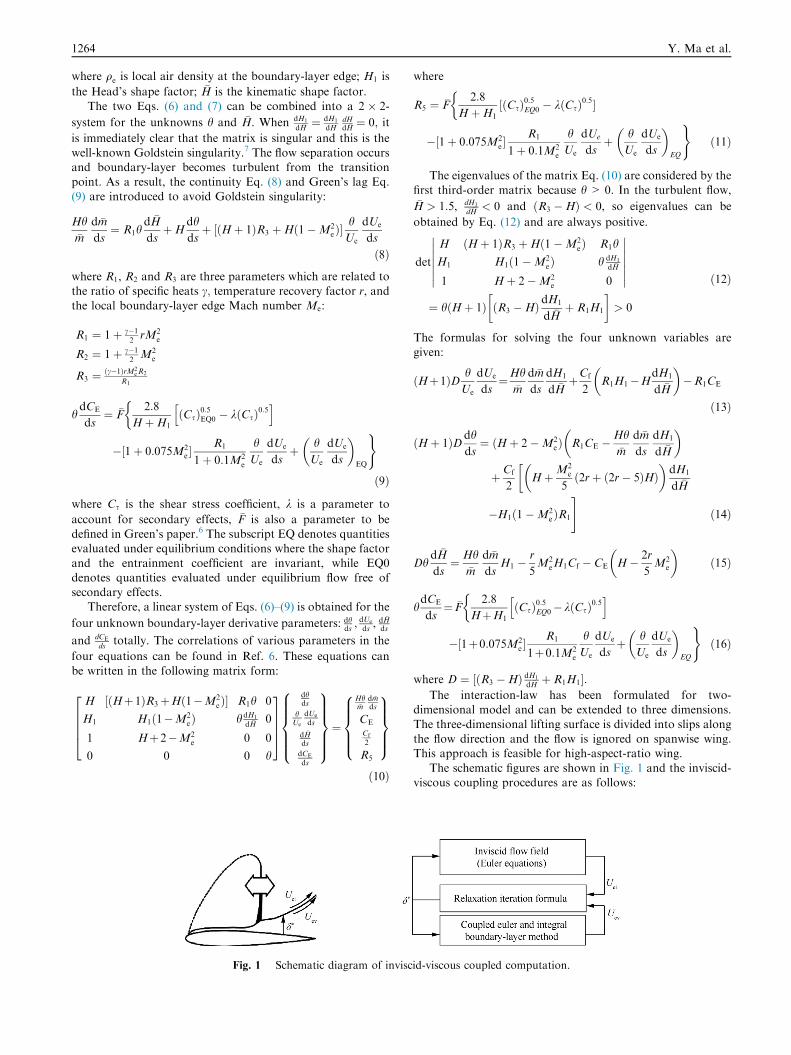
The interaction-law has been formulated for two-dimensional model and can be extended to three dimensions.

The three-dimensional lifting surface is divided into slips alongthe flow direction and the flow is ignored on spanwise wing.This approach is feasible for high-aspect-ratio wing.

The schematic figures are shown in Fig. 1 and the inviscid-viscous coupling procedures are as follows:

id-viscous coupled computation.

Wing aeroelasticity analysis based on an integral boundary-layer method coupled with Euler solver 1265

(1) Initial thickness of boundary-layer distribution d*(s) isgiven in advance. The Eqs. (13)–(16) are employed to

solve each boundary-layer variable �H , h, and Uev.(2) The blowing velocity V b can be obtained from mass

conservation:

Vb ¼ d

qedsðqeUevd

�Þ ð17Þ

The blowing velocity Vb is used considering the viscouseffect in the Euler solver, which is implemented as the

simplified boundary condition6 for the unsteady andaeroelastic computations.

(3) The outer boundary-layer speed U ei is solved by Euler

equations after 15–50 iteration steps.(4) The boundary-layer thickness is updated by relaxation

scheme:

Carter’s formula:

d�new ¼ d�old 1þ xUev

Uei

� 1

� �� �ð18Þ

Edward’s formula:

d�new ¼ d�old þ xDsðUev �UeiÞ ð19ÞHere, x is an under-relaxation factor and is usually taken

0.1–0.2. Each of the two relaxation schemes has its own advan-

tages and disadvantages, so users need to choose according todifferent models and calculating states. The Carter’s schemeconverges quickly, but the calculation stability is not high

and easy to diverge on the separation flow. The Edward’sscheme is more stable, but relatively has slow convergencespeed. So we can first apply the Carter’s scheme to a small resid-

ual value, and then use Edward’s scheme until it converges.Convergence is judged from the difference between the two

boundary-layer edge velocities Uev and Uei ( d�new � d�old

���� 6 e).If it is true, the calculation process will stop. Conversely, d�oldwill be replaced by d�new; and then the program will jump to

step (2) and continue to calculate until results converge.

2.3. Solution procedure for static aeroelastic analyses

The dynamic response of structure is analyzed by the modesuperposition method. The motion of forced vibration ofmulti-degree-of-freedom system can be obtained from the

physical characteristics of the system:

M€qþ Kq ¼ F ð20Þwhere M is the generalized mass matrix; K is the generalizedstiffness matrix; F is the generalized aerodynamic force matrix;

q is the generalized displacement.Furthermore, an iterative procedure Eqs. (21)–(25) can be

used to get an updated generalized force F:

dðjÞ ¼ UqðjÞ ð21Þ

F ¼ UTQ1fðdðjÞ; aÞ ð22Þ

K~qðjþ1Þ ¼ F ð23Þ

D~qðjÞ ¼ ~qðjþ1Þ � qðjÞ ð24Þ

qðjþ1Þ ¼ qðjÞ þ �kD~qðjÞ ð25Þwhere U is the displacement interpolation matrix from struc-ture grids to aerodynamic grids; Q1 is the dynamic pressure;

fðdðjÞ; aÞ is the force vector of aerodynamic model’s surface grid.

The iterative process must be iterated until jD~qðjÞj is equal todesired tolerance. �k is relaxation factor and 0.2–0.6 is chosen to

ensure iteration converge. If it does not converge nomatter how

small �k is, then the analysis of static aeroelasticity is divergent.

2.4. Solution procedure for flutter analyses

Eq. (20) is also applied to solving the flutter problem. We

introduce the state-space variables X ¼ ½q; _q�T; and Eq. (20)can be rewritten in state-space form:

_X ¼ AXþ BF

A ¼ 0 I

�M�1K �M�1C

� �;B ¼ 0

M�1

� �8<: ð26Þ

The Runge-Kutta method is applied to solving the differentialEq. (26) and its expansion is given by

Xnþ1 ¼ Xn þ ðk1 þ 2k2 þ 2k3 þ k4Þ=6k1 ¼ Dt½AXn þ BFðXn; tnÞ�k2 ¼ Dt½AðXn þ k1=2Þ þ BFðXn þ k1=2; tn þ Dt=2Þ�k3 ¼ Dt½AðXn þ k2=2Þ þ BFðXn þ k2=2; tn þ Dt=2Þ�k4 ¼ Dt½AðXn þ k3Þ þ BFðXn þ k3; tn þ DtÞ�

8>>>>>>><>>>>>>>:

ð27Þ

When computations are performed on a loosely coupledmodel, the aerodynamic forces FðXn þ k1=2; tn þ Dt=2Þ and

FðXn þ k2=2; tn þ Dt=2Þ are unknowns except FðXn; tnÞ. If theseunknowns are substituted by FðXn; tnÞ, the coupled method isonly of first-order time accuracy. Therefore, the time step mustkeep small enough to satisfy the accuracy requirement.

The aerodynamic forces Ft�2Dt, Ft�Dt and Ft (at time stepst� 2Dt, t � Dt and t) can be fitting out a quadratic curve, sothat the numerical extrapolated method is employed at time

tþ Dt=2 and t+ Dt:

FtþDt=2 ¼ ð15Ft � 10Ft�Dt þ 3Ft�2DtÞ=8FtþDt ¼ 3Ft � 3Ft�Dt þ Ft�2Dt

�ð28Þ

Substituting Eq. (28) into the equation for the Runge-Kutta

expansion, Eq. (27), yields

Xnþ1 ¼ Xn þ ðk1 þ 2k2 þ 2k3 þ k4Þ=6k1 ¼ Dt½AXn þ BFðXn; tnÞ�k2 ¼ Dt½AðXn þ k1=2Þ þ BFtþDt=2�k3 ¼ Dt½AðXn þ k2=2Þ þ BFtþDt=2�k4 ¼ Dt½AðXn þ k3Þ þ BFtþDt�

8>>>>>>>><>>>>>>>>:

ð29Þ

The Eq. (29) provides second-order time accuracy and thetime step can be increased moderately, which can improvethe efficiency of the computation.21 Loosely coupled solution

scheme can be seen as a serial staggered procedure for flutteranalyses in Fig. 2, in which qt is the generalized displacement

and Vtb is the blowing velocity at time steps t.

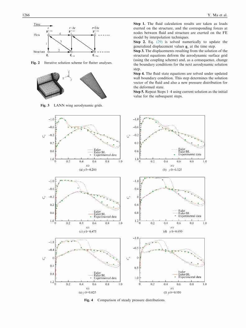
Fig. 4 Comparison of stead

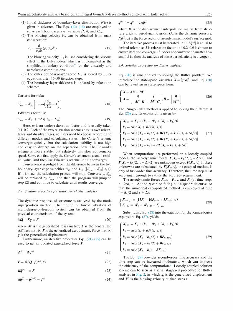
Fig. 3 LANN wing aerodynamic grids.

Fig. 2 Iterative solution scheme for flutter analyses.

1266 Y. Ma et al.

Step 1. The fluid calculation results are taken as loads

exerted on the structure, and the corresponding forces atnodes between fluid and structure are exerted on the FEmodel by interpolation techniques.

Step 2. Eq. (29) is solved numerically to update thegeneralized displacement values qn at the time step.Step 3. The displacements resulting from the solution of thestructural equations deform the aerodynamic surface grid

(using the coupling scheme) and, as a consequence, changethe boundary conditions for the next aerodynamic solutionstep.

Step 4. The fluid state equations are solved under updatedwall boundary condition. This step determines the solutionvector of the fluid and also a new pressure distribution for

the deformed state.Step 5. Repeat Steps 1–4 using current solution as the initialvalue for the subsequent steps.

y pressure distributions.

Wing aeroelasticity analysis based on an integral boundary-layer method coupled with Euler solver 1267

3. Static aeroelastic calculation and analysis

3.1. Steady flow validation

The sections of the LANN wing are supercritical airfoils fromthe AGARD R-702 report. The wing is twisted from 2.6� at theroot section and �2� at the tip section. The aspect ratio of thewing is 7.92. The taper ratio is 0.4 and the quarter-chord sweptangle is 25�.22 C–H grids are used for the Euler and Euler/BL

computations which totally include 527,280 spatial grids and1960 surface grids as shown in Fig. 3.

The steady flow field is computed and used as the initialflow field for the unsteady computation. The Mach number

Ma is 0.822; the angle of attack a is 0.6; the experimentalReynolds number based on root chord is 20.27 � 106. Fig. 4shows the comparisons of the calculated and experimental sur-

face pressures, where b is the half span. The results obtainedfrom the current Euler/BL method are fairly consistent withthe experimental data. The shock position is shifted forward

and the strength is weakened compared with the Eulersolutions.

3.2. HIRENASD wing finite element model and structured gridsof flow field

The high Reynolds number aero-structural dynamics(HIRENASD) project23,24 was led by the Aachen

Fig. 5 HIRENASD schematic structure of finite element model.

Fig. 6 HIRENASD wing aerodynamic grids.

University with funding from the German Research Foun-dation. It was initiated in 2004 to produce a high-qualitytransonic aeroelastic data set at realistic flight Reynolds

numbers for a large transport-type wing/body configura-tion and tested in the European transonic wind tunnel(ETW) in 2006. Therefore, detailed experimental data

can be provided for static aeroelastic validation of thisstudy.

The finite element model (FEM) of the HIRENASD wing

is modeled with solid elements and composed of NASTRANhexagonal elements with over 200,000 grid points as shownin Fig. 5. The first ten oscillating frequencies and oscillatingmodes are chosen for calculation.

The flow field of the spatial grids and surface gridsabout the HIRENASD wing is shown in Fig. 6. Thenumber of spatial grids is 855,108 and that of surface

grids is 7750.

3.3. Static aeroelastic results and analysis

As mentioned in Section 2, the iterative process Eqs. (21)–(25) is applied to calculating static aeroelastic deformationof the wing (Ma= 0.80, a = 1.5 and Re = 7 � 106). The

HIRENASD experimental steady pressure data are collectedat six span sections, which are identified in Fig. 7. Fig. 8 pre-sents the distribution pressure coefficient (Cp) results at sixsections obtained from the rigid steady (undeformed) and sta-

tic aeroelastic (deformed) solutions. The trend of Cp is consis-tent with the experimental results and deformed surfacepressure is closer to the experimental values than that in

the rigid case.The wing tip displacements are calculated at five angles of

attack (�1.5�, 0.0�, 1.5�, 3.0� and 4.5�) and compared with

experimental data shown in Fig. 9.25,26 The calculated dis-placements for HIRENASD are slightly less than experimentaldata.

The analysis of static aeroelasticity based on anintegral boundary-layer method is developed. The results showthat:

(1) Deformed pressure distributions are more consistentwith experimental results.

(2) Compared with the experimental data, the process of

static aeroelasticity is feasible and can be used forhigh-aspect-ratio wing.

Fig. 7 HIRENASD span sections 1–6.

Fig. 8 Comparison of rigid steady and static aeroelastic surface pressure distributions.

Fig. 9 Wing tip displacements for HIRENASD, Ma = 0.8,

Re = 7 million.

1268 Y. Ma et al.

4. Flutter calculation and analysis

4.1. Unsteady flow validation

The LANN wing is also used to test the accuracy in unsteadycase. The wing oscillates around an upswept axis at 62.1% ofthe root chord in a pitch motion as

aðtÞ ¼ a0 þ am sinðwtÞ ð30ÞIn this case, the mean angle of attack a0 is 0.6; the pitching

amplitude am is 0.25; the reduced frequency j is 0.204. In orderto compare the pressure distribution of the unsteady

computation, the Fourier transformation is used. The firstmode of the normalized pressure distribution at six span posi-tions is shown in Fig. 10.

Fig. 10 Comparison of unsteady pressure distributions.

Wing aeroelasticity analysis based on an integral boundary-layer method coupled with Euler solver 1269

Similar to the results of steady computation, the Eulersolver over-predicts the shock wave position. The abrupt

change can be seen in the unsteady pressure distributionsat every position in Fig. 10, corresponding to the positionof the shock wave in Fig. 4, where the shock wave changesthe unsteady flow. The Euler/BL method well compensates

the shortcomings that viscosity cannot be considered inEuler equations. When the shock wave appears on thesurface of wing, the unsteady pressure distributions will

bulge.

4.2. AGARD 445.6 wing

The AGARD 445.6 wing was tested in the NASA LangleyTransonic Dynamics Tunnel (TDT) in 1961. Flutter data fromthis test have been publicly available for over 20 years and

have been widely used for preliminary computational aeroelas-tic benchmarking. In this section, the results of the AGARD445.6 wing are presented in order to validate the Euler/BL

method for flutter calculations. The wing is semi-span with aquarter-chord sweep angle of 45�, an aspect ratio of 1.65, a

Fig. 10 (continued)

Fig. 11 AGARD 445.6 wing aerodynamic grids.

1270 Y. Ma et al.

Fig. 13 Computed flutter results for AGARD wing.

Fig. 12 Time histories of generalised displacements of AGARD 445.6 wing at Ma = 0.901.

Wing aeroelasticity analysis based on an integral boundary-layer method coupled with Euler solver 1271

taper ratio of 0.66, and a NACA 65A004 airfoil section whichis a symmetric airfoil.27 Its detailed parameters can be

obtained in wind tunnel test report and the first four orderoscillating modes were used in flutter analysis.

The surface grids of AGARD 445.6 wing and the structural

computational grids are depicted in Fig. 11. The spatial gridsare 237,600; the surface grids are 24,192.

4.3. Flutter results and analysis

In order to illustrate the effect of boundary-layer correction,two methods are employed to calculate flutter of AGARD445.6 wing at free stream (Ma= 0.500, 0.678, 0.901, 0.960,

1.072 and 1.141). Moreover, the generalized displacementscomputed by the Euler method at Ma= 0.901 are shown inFig. 12. Fig. 13 presents comparisons of the experimental flut-

ter speeds and frequency ratio values and N-S solver resultsobtained using the FUN3D code27 are also compared.

The analysis of flutter based on an integral boundary-layer

method is developed:

(1) The calculation results of three methods are consistent

with the transonic dip of AGARD 445.6 wing nearMa= 0.960;

(2) The results of the Euler/BL method are better than thoseof the Euler solver and less than those of N-S methods;however, the calculation is more efficient than that of N-S equations. It is thus more suitable for industrial design

environment.

5. Conclusions

An Euler/BL method has been developed to calculate unsteady

flow and aeroelastic problems in detail. Three examples arepresented to demonstrate the approach and the following con-clusions can be drawn:

(1) The study firstly shows that the results obtained by theEuler/BL method are better than the Euler results in

both steady and unsteady cases.(2) A process of static aeroelastic analysis is verified, which

is implemented on the HIRENASD wing. The develop-ment of flutter process is also verified by the AGARD

445.6 wing.(3) It is concluded that the viscous effects are significant for

these cases and further data analysis demonstrates the

presented method’s validity and practicability. Themethod can be used to solve aeroelastic problems.

1272 Y. Ma et al.

Acknowledgements

This study was co-supported by the National Natural Science

Foundation of China (No. 51675426) and Aerospace Scienceand Technology Innovation Fund of China (No.2014KC010043).

References

1. Dowell EH, Hall KC. Modeling of fluid-structure interaction.

Annu Rev Fluid Mech 2001;33(1):445–90.

2. Chen PC, Liu DD, Karpel M. ZAERO User’s Manual. ZONA

Technology; 2006. p. 1–10.

3. Tang L, Bartels R, Chen P, Liu DD. Numerical investigation of

transonic limit oscillations of a 2-D supercritical wing. Reston:

AIAA; 2001. Report No.: AIAA-2001-1290.

4. Thomas JP, Dowell EH, Hall KC. Nonlinear in viscid aerody-

namic effects on transonic divergence, flutter, and limit-cycle

oscillations. AIAA J 2002;40(4):638–46.

5. Geissler W. Numerical study of buffet and transonic flutter on the

NLR 7301 airfoil. Aerosp Sci Technol 2003;7(7):540–50.

6. Zhang ZC, Liu F. Calculations of unsteady flow and flutter by an

Euler and integral boundary-layer method on Cartesian grids.

Proceedings of the 22nd applied aerodynamics conference and

exhibit; 2004 August 16–19; Rhode Island, USA. Reston: AIAA;

2004. p. 1–13.

7. Lock RC, Williams BR. Viscous-inviscid interactions in external

aerodynamics. Prog Aerosp Sci 1987;24(2):51–171.

8. Sturdza P, Suzuki Y, Martins-rivas H, Rodriguez DL. A quasi-

simultaneous interactive boundary-layer model for a cartesian euler

solver. Proceedings of the 50th AIAA aerospace sciences meeting

including the new horizons forum and aerospace exposition; 2012

January 09–12; Nashville, USA. Reston: AIAA; 2012. p. 1–20.

9. Rodriguez DL, Sturdza P. Improving the accuracy of euler/

boundary-layer solvers with anisotropic diffusion methods. Pro-

ceedings of the 50th AIAA aerospace sciences meeting including

the new horizons forum and aerospace exposition; 2012 January

09–12; Nashville, USA. Reston: AIAA; 2012. p. 1–15.

10. Drela M. Three-dimensional integral boundary layer formulation

for general configurations. Proceedings of the 21st AIAA compu-

tational fluid dynamics conference; 2013 June 27–30; San Diego,

USA. Reston: AIAA; 2013. p. 1–24.

11. Nishida B, Drela M. Fully simultaneous coupling for three-

dimensional viscous/inviscid flows. Reston: AIAA; 1995. Report

No.: AIAA-95-1806.

12. Veldman AEP. A simple interaction law for viscous-inviscid

interaction. J Eng Math 2009;65(4):367–83.

13. Carter JE. A new boundary-layer inviscid iteration technique for

separated flow. Reston: AIAA; 1979. Report No.: AIAA-1979-

1450.

14. Potsdam MA. An unstructured mesh Euler and interactive

boundary layer method for complex configurations. Reston:

AIAA; 1994. Report No.: AIAA-94-1844.

15. Gao C, Luo S, Liu F, Schuster DM. Calculation of unsteady

transonic flow by an Euler method with small perturbation

boundary conditions. In: Proceedings of the 41st aerospace

sciences meeting and exhibit; 2003 January 6–9; Reno, USA.

Reston: AIAA; 2003. p. 1–13.

16. Gao C, Yang S, Luo S, Liu F, Schuster DM. Calculation of airfoil

flutter by an Euler method with approximate boundary condi-

tions. AIAA J 2005;43(2):295–305.

17. Rodden WP, Johnson EH. MSC/NASTRAN Aeroelastic analysis

user’s guide, Version 68. Los Angeles: The Macneal-Schwender

Corporation; 1994.

18. Relvasa A, Suleman A. Fluid–structure interaction modelling of

nonlinear aeroelastic structures using the finite element corota-

tional theory. J Fluid Struct 2006;22(1):59–75.

19. Cohen CB, Cresci RJ. The compressible laminar boundary layer

with heat transfer and pressure gradient. Washington, D.C.:

NASA; 1956. Report No.: NACA TR-1294.

20. McNally WD, FORTRAN Program for calculating compressible

laminar and turbulent boundary-layers in arbitrary pressure

gradients. Washington D.C.: NASA; 1979. Report No.: NASA

TND-5681.

21. Zhang WW. Efficient analysis for aeroelasticity based on compu-

tational fluid dynamics. [dissertation] Xi’an: Northwestern

Polytechnical University; 2006 (Chinese).

22. Zwaan R. LANN wing pitching oscillation, compendium of

unsteady aerodynamics measurements. London RH: AGARD;

1982. Report No.: AGARD-R-702.

23. Acar P, Nikbay M. Steady and unsteady aeroelastic computations

of HIRENASD wing for low and high Reynolds numbers.

Proceedings of the 54th AIAA/ASME/ASCE/AHS/ASC struc-

tures, structural dynamics, and materials conference; 2013 April 8–

11; Boston, USA. Reston: AIAA; 2013. p. 1–16.

24. Chwalowski P, Florance JP. Heeg J, Wieseman CD, Perry B.

Preliminary computational analysis of the (HIRENASD) config-

uration in preparation for the aeroelastic predication workshop.

International forum of aeroelasticity and structural dynamics;

2011 June 26–30; Paris, France. 2012. p. 1–21.

25. Ritter M. Static and forced motion aeroelastic simulations of the

HIRENASD wind tunnel model. Proceedings of the 53rd AIAA/

ASME/ASCE/AHS/ASC structures, structural dynamics and

materials conference; 2012 April 23–26; Honolulu, USA. Reston:

AIAA; 2012. p. 1–14.

26. Ballmann J, Dafnis A, Korsch H, Buxel C, Reimerdes HG.

Experiment analysis of high Reynolds number aero-structural

dynamics in ETW. Proceedings of the 46th AIAA aerospace

sciences meeting and exhibit; 2008 January 7–10; Reno, USA.

Reston: AIAA; 2008. p. 1–15.

27. Lee-Rausch EM, Batinaf JT. Wing flutter computations using an

aerodynamic model based on the Navier-Stokes equations. J Aircr

1996;33(6):1139–47.

Ma Yanfeng is a Ph.D. student at School of Aeronautics, Northwest-

ern Polytechnical University. Her area of research is aircraft aeroe-

lasticity.

He Erming is a currently professor at School of Aeronautics, North-

western Polytechnical University. He received the Ph.D. degree from

the same university in 1993. His major research interests are vibration

and control design of aircraft structure.