Window Dressing of Short-Term Borrowingsutah-wac.org/2012/Papers/owens_UWAC.pdf · 2012-02-15 ·...

Window Dressing of Short-Term Borrowings◊

Edward L. Owensa and Joanna Shuang Wub

William E. Simon Graduate School of Business Administration, University of Rochester, Rochester, NY 14627, United States

February 2012 First Draft: March 2011

_______________________________ ◊

We thank Jose Berrospide, Dan Collins, Anya Kleymenova, Anzhela Knyazeva, Stephen Ryan, Jerry Zimmerman, and workshop participants at George Washington University, London Business School, New York University, University of Rochester, the University of Minnesota 2011 Empirical Research Conference, and the Fifth Annual Toronto Accounting Research Conference for helpful comments and suggestions. a Tel.: +15852751079; email: [email protected]. b Tel.:+15852755468; email: [email protected].

Window Dressing of Short-Term Borrowings

Abstract

We investigate bank holding companies’ window dressing of quarter-end short-term borrowings. We find evidence of downward window dressing of short-term borrowings through repo and federal funds liabilities that appears material for a large fraction of the sample. Such downward window dressing is more pronounced at banks with a higher concentration of short-term borrowings in their total liability structure and lower capital adequacy ratios, consistent with risk-masking incentives. Such window dressing is also more pronounced at banks with greater management compensation sensitivity to ROA and at banks that borrow in private debt markets, consistent with contractual incentives. Finally, we document a negative equity market reaction to the release of regulatory filings that indicate unexpected downward window dressing of short-term borrowings. The potential implications of our findings go beyond bank holding companies and the financial industry, and bear relevance to recent SEC deliberations regarding short-term borrowing disclosure regulation.

JEL Classification: G14; G21; G28; M40 Keywords: Window dressing; Short-term borrowing; Sale and repurchase agreement; Bank holding companies; Disclosure regulation

1

1. Introduction

The recent financial crisis brought into focus financial institutions’ risk-taking behavior,

and raised concerns about whether their end-of-quarter balance sheets are accurate depictions of

their risk levels during the quarter.1 Coincident with these concerns, the Securities and Exchange

Commission (SEC) unanimously voted on September 17, 2010 to propose rules requiring both

financial and non-financial public companies to provide enhanced disclosure of short-term

borrowings such as repurchase agreements (repos), federal funds purchased, and commercial

paper.2 The SEC is particularly concerned with disclosures related to short-term borrowings, as

the levels of such borrowings can vary significantly during a reporting period, potentially making

end-of-period balances less representative of risk exposure during the period. Moreover, the SEC

points out that short-term borrowings form a critical component of firms' liquidity and capital

resources, and that recent events have shown that such sources of funding can be severely

affected by market illiquidity.

Even though the spotlight has been on the financial industry, similar issues can arise in

other industries that rely on short-term financing arrangements to fund operations. In its

proposed rule, the SEC suggests that the inherent riskiness associated with short-term

borrowings may warrant enhanced disclosure of within-quarter exposure to these risks by all

SEC registrants. Presently, only commercial banks and bank holding companies (BHCs) are

required to disclose quarterly averages of certain financial variables, including a key source of

their short-term funding - repurchase agreements and federal funds. Appendix A summarizes the

1 For example, a Wall Street Journal article on April 9, 2010 titled “Big banks mask risk levels” reports that during 2009 a group of 18 large banks in aggregate substantially lowered their quarter-end repo liabilities compared to the levels during the quarter. 2 SEC Release Nos. 33-9143 and 34-62932 (Sept. 17, 2010); File No. S7-22-10 (to be codified at 17 C.F.R Parts 229 and 249).

2

current disclosure requirements for BHCs from the Federal Reserve and the SEC as well as the

SEC’s proposed rule.

In this study, we investigate BHCs' downward window dressing of quarter-end short-term

borrowings, where we define window dressing as a discretionary short-term deviation around

quarter-end reporting dates of a financial variable from its quarterly average level.3 In so doing,

this study provides the first empirical evidence on the window dressing of short-term borrowings

and the stock market reaction to the public release of regulatory filings (i.e., Y-9C filings) from

which window dressing may be detected. Even though our analysis is based on Y-9C filings by

BHCs, the implications are broader and may extend to other industries.

Incentives for managers to downward window dress short-term borrowings can come

from several sources. First and foremost, as pointed out by the SEC short-term borrowings such

as repo liabilities are inherently risky. In particular, when market liquidity is low, firms that rely

heavily on short-term borrowings are more susceptible to increases in borrowing rates or other

unfavorable terms. Further, when markets are unstable it may be difficult to roll over short-term

borrowings. Therefore, banks may have a direct incentive to decrease the reported quantity of

such short-term borrowings in their financial statements, ceteris paribus. Managers may thus

engage in downward window dressing in an attempt to mask the true risk level of the firm in

hopes of obtaining higher valuations for the firms' securities and better terms with transaction

counterparties. Second, regulatory capital requirements may provide both direct and indirect repo

liability window dressing incentives. A direct incentive comes from the fact that the amount of

margin ("haircut") in a repo transaction imposes additional risk-based capital requirements on the

borrower. Therefore, banks may decrease their repo borrowings around quarter-end to directly

3 We describe our empirical measure of window dressing in detail in Section 4.1. As is standard in the literature, we refer to cases where the quarter-end value is less than (greater than) its quarterly average level as downward (upward) window dressing.

3

reduce required risk-based capital. Indirectly, banks with lower capital adequacy ratios appear

riskier, and therefore may have added incentive to reduce their disclosed levels of risky short-

term borrowings. Finally, window dressing may arise from contractual incentives. By taking on

additional borrowing during the quarter, a bank expands its balance sheet and the base from

which earnings are produced. If managers and other employees are compensated based on

earnings relative to the end-of-quarter asset base and risk levels, downward window dressing of

short-term borrowings can boost their compensation relative to compensation that would be

awarded in the absence of window dressing. Furthermore, participation as a borrower in private

debt markets can provide an additional window dressing motive because of a desire to avoid

financial covenant violations.

Using a sample of publicly traded BHCs, we find evidence of significant downward

deviations in quarter-end short-term borrowings levels, in particular, repo and federal funds

liability accounts, that appear material in a substantial fraction of firm-quarter observations,

especially among the largest BHCs. Consistent with our predictions, we find that BHCs with a

higher concentration of short-term borrowings in their liability structure (i.e., those that likely

have greater incentives to mask their risk levels) have larger downward deviations in quarter-end

repo and federal funds liabilities. In addition, we find evidence that the magnitude of these

quarter-end downward deviations is greater for relatively large BHCs with lower regulatory

capital adequacy ratios. We further document the magnitude of downward quarter-end deviations

in short-term borrowings is larger for banks with greater sensitivity of CEO total compensation

to return on assets, a performance measure typically used in compensation contracts that may be

boosted by window dressing activities. Finally, we provide some evidence that such downward

window dressing is more pronounced for firms that borrow in the private debt market.

4

We consider the possibility that the short-term deviation of repo and federal funds

liabilities around quarter-end reporting dates from its quarterly average level is driven by bank

counterparties (i.e., repo and federal funds lenders and/or bank customers) rather than banks’

own discretion. For example, repo and federal funds lenders may themselves face greater

funding needs for operations around quarter ends and therefore temporarily reduce their supply

of funds. We examine market-wide repo lending rates and document that repo rates decline

shortly before quarter end and bounce back immediately after, which is consistent with a

reduction in borrower demand right before quarter ends, rather than a reduction in lender supply.

In terms of the potential effects from bank customers, we investigate within quarter

changes in bank deposits and loans. If deposits systematically increase at quarter ends, it can

reduce the banks’ needs for borrowing in the repo and federal funds markets. We address this

concern by controlling for quarter-end deviations of bank deposits from their quarterly averages

and find our results robust to this control. There is also the possibility that borrowers from the

bank may return part of the loans to window dress their own balance sheets before quarter ends

and the additional funding from returned loans allow the bank to unwind portions of its own repo

and federal funds borrowings. We compare quarterly averages of loans with the quarter-end loan

balances and find no evidence that loan balances are systematically lower at quarter ends, in fact,

they tend to be higher. This is inconsistent with systematic repayments of loans around quarter

ends.4 Finally, we note that customer-driven activities should not be systematically associated

with bank risk characteristics, absent the banks' own incentives to mask risks. Our evidence that

downward quarter-end deviations in repo and federal funds liabilities intensifies for banks with a

higher concentration of short-term borrowings, lower capital adequacy ratios, and tighter

4 This result is based on a small sample of observations because information on quarterly averages of loans was not available prior to 2010 and thus should be interpreted with caution.

5

correlation between ROA and compensation is therefore difficult to explain from a counterparty

perspective, and is more consistent with BHC-initiated window dressing of short-term

borrowings. We consider several other alternative explanations for our findings, including

window dressing of risky assets and reserve requirement measurement periods. We conclude that

these factors are likewise unlikely to account for our findings.

We assess the stock market reaction around the public release of BHC quarterly Y-9C

filings, from which potential window dressing can be detected. We find that unexpected

downward quarter-end deviations in repo and federal funds liabilities is associated with

significantly lower Y-9C announcement period stock returns, which suggests that such window

dressing induces negative updates in investor beliefs regarding true risk levels, earnings

performance, and/or management quality and integrity. We caution that these results do not

speak to whether downward window dressing of repo and federal funds liabilities is on net

beneficial or detrimental to the shareholder wealth, because positive market reactions to the

results of such window dressing, including higher capital adequacy ratio, higher ROA, and lower

probability of covenant violations, may have already been impounded into share prices from

earlier management communications regarding accounting earnings and certain important

quarter-end balance sheet items before the release of the Y-9C.

Our evidence on window dressing is not necessarily indicative of accounting

improprieties such as those that allegedly occurred with Lehman Brothers’ “Repo 105”

transactions (Valukas, 2010), which involve recording repo borrowings as security sales rather

than liabilities. Such practices, if present in our sample, would only be captured by our window

dressing measure if they are strategically timed around quarter end. It is more likely that our

measure reflects window dressing behavior where BHCs unwind a portion of their within-quarter

6

repo and federal funds borrowings before quarter end, and then resume borrowing early in the

following quarter. Such activities involve changes in real borrowing activities and are not illegal

or in violation of any current accounting standards. Nevertheless, such actions understate the

risks presented by the bank's use of short-term borrowings during the quarter.

We make several contributions to the literature. Our study is the first to provide empirical

evidence of window dressing of short-term borrowings, an issue that has received heightened

media and regulatory attention. Our findings confirm anecdotal evidence on the existence of such

behavior and validate the concerns behind the new proposed SEC rule on “Short-Term

Borrowing Disclosure.” We provide insights into the incentives behind such window dressing

behavior and how it varies across firms and over time. Our market test indicates that investors

react to information on quarterly averages in short-term borrowing accounts such as repo and

federal funds, which suggests that investors will likely benefit from the new SEC proposed

“Short-Term Borrowing Disclosure” rule for firms that are not currently subject to such

disclosure requirements.5 Finally, we note that window dressing of short-term borrowings may

be related to window dressing of risky assets and current disclosures of quarterly averages on the

asset side in the Y-9C report do not allow clear inferences regarding risky asset window

dressing.

The remainder of the paper is organized as follows. Section 2 discusses related literature

and provides background on Y-9C filings by bank holding companies and the repo and federal

funds markets. Section 3 develops the paper’s predictions. Section 4 outlines the research design.

Section 5 describes our sample selection and summary statistics, and Section 6 presents our

empirical results. Section 7 concludes.

5 Our analysis does not address whether the new SEC proposed rule will be on net beneficial or costly. Such an assessment requires a comprehensive analysis of the potential benefits as well as costs of the new regulation, which is beyond the scope of this study.

7

2. Background

2.1. Related literature

Window dressing is often characterized as an action taken by an agent that "improves the

agent's performance measure but contributes little or nothing to the principal's gross payoff"

(Feltham and Xie, 1994). Extant literature has examined window dressing in various settings.

One stream of research documents that fund managers and institutional investors dress up their

quarter-end or year-end portfolio holdings by selling losing stocks and buying winning stocks

(e.g., Lakonishok et al., 1991; Musto, 1999; He et al., 2004; Ng and Wang, 2004). Dechow and

Shakespeare (2009) find that managers time securitization transactions towards the end of the

quarter to increase earnings, improve efficiency ratios, and reduce leverage.

Two papers of note have looked at window dressing in the banking sector, where both

studies point out that differences between a bank's quarter-end and within-quarter levels of

financial variables may be initiated either by the bank itself ("active" window dressing) or by

parties external to the bank, such as customers ("passive" window dressing). Allen and Saunders

(1992) find evidence of upward window dressing of bank total assets, which they attribute to

managers’ incentives to inflate bank size in order to be viewed as “too-big-to-fail” and/or to

enhance managerial compensation and non-pecuniary reputational benefits. Kotomin and

Winters (2006), on the other hand, argue that the upward window dressing of bank total assets is

more likely customer-driven rather than a reflection of bank discretion. Both studies focus on the

rationales behind upward window dressing of bank total assets and do not look specifically at

possible downward window dressing in short-term borrowings. In addition, both studies examine

commercial banks rather than BHCs, where they obtain data from commercial bank Call Reports

8

and H.8 releases, respectively.6 However, many of the financial institutions where window

dressing of short-term borrowings is a concern are not pure commercial banks. Moreover, an

important objective of our paper is to assess the market reaction to such window dressing.

Therefore, a focus on BHCs is more appropriate for purposes of our study. Furthermore, whereas

the sample periods in Allen and Saunders (1992) and Kotomin and Winters (2006) are 1978-

1986 and 1994-2002, respectively, our sample period of 2001-2010 is more pertinent to recent

economic events.

2.2. FR Y-9C reporting by bank holding companies

At the end of 2009, there were 5,634 U.S. BHCs in operation, which controlled 5,710

commercial banks and held approximately 99% of all insured commercial bank assets in the U.S.

(Board of Governors of the Federal Reserve Annual Report, 2009).7 Domestic BHCs with total

consolidated assets of $500 million or more are required under Federal Reserve Board

Regulation Y and the Bank Holding Company Act of 1956 (as amended) to file form FR Y-9C

with the Federal Reserve as of the last day of each calendar quarter.8 Form Y-9C contains

detailed information on BHCs' consolidated financial statements and regulatory capital,

including numerous supporting schedules. Schedule HC-K contains disclosures of quarterly

averages for select balance sheet items calculated on a daily or weekly basis, thus enabling

detection of quarter-end deviations from quarterly averages by comparison of the quarterly

average amounts with quarter-end values of corresponding financial items found elsewhere in the 6 Unlike the Y-9C, the Call Report does not provide quarterly averages of shareholders’ equity, which prevents the calculation of quarterly average financial leverage. The H.8 data has the disadvantage of being at the aggregate level instead of firm-specific. 7 The Bank Holding Company Act of 1956 defines a bank holding company as any company (including a commercial bank) that has direct or indirect control of a commercial bank. “Control” means ownership, control, or power to vote 25 percent or more of the outstanding shares of any class of voting securities of the bank, or control in any manner over the election of a majority of the directors, trustees, or general partners of the bank, or the power to exercise a controlling influence over the management or policies of the bank. 8 The reporting size threshold was $150 million prior to 2006. Furthermore, only the top-tier BHC within a BHC hierarchy is required to file Y-9C post-2006. Previously, all BHCs that satisfy the size threshold must file.

9

Y-9C.9 BHCs are required to disclose quarterly averages for three types of liability accounts: i)

deposits, ii) repo and federal funds purchased, and iii) "other borrowed money." For our sample,

about 80% of the balance in repo and federal funds purchased reflects repo transactions. "Other

borrowed money" consists of commercial paper, other short-term borrowed money, and other

long-term borrowed money. The long-term component makes up the majority, roughly 80%, of

“other borrowed money.” Liability accounts for which quarterly averages are not provided in the

Y-9C include trading liabilities, subordinated notes and debentures, and other liabilities (e.g.,

deferred taxes). BHCs are required to disclose quarterly averages for six asset categories: i)

securities, ii) repo and federal funds sold, iii) total loans and leases, iv) trading assets, v) other

earning assets, and vi) total consolidated assets. Finally, banks must disclose quarterly average

total equity capital. BHCs are required to file Form Y-9C within 40 days after quarter end for the

first three calendar quarters and within 45 days after the fourth calendar quarter end. Y-9C

reports are generally publicly available 42 days after the end of the first three calendar quarters,

and 47 days after the fourth calendar quarter end on the Federal Reserve National Information

Center website.10

2.3. Repo and federal funds markets

Repo and federal funds liabilities are likely to be the most convenient vehicles for

window dressing of short-term borrowings for most BHCs. A repo, also known as sale and

repurchase agreement, is essentially a collateralized loan. The borrower receives cash from the

lender and transfers to the lender securities as collateral. It is agreed up front that the securities 9 Interestingly, extant literature suggests that bank regulators and the SEC have neither devoted large amounts of resources to monitor window dressing activities revealed in bank regulatory filings, nor imposed severe penalties when such activities are detected (Allen and Saunders, 1992). Internal statistics from the Federal Reserve are consistent with window dressing-related enforcement actions against banks being infrequent and bearing relatively minor consequences. For example, in 2009 the Federal Reserve completed 191 formal enforcement actions and assessed a total of $249,570 in civil penalties against the entire set of banking organizations it supervises for all categories of unsound practices and/or regulatory violations combined (BOG of the Fed Annual Report, 2009). 10 http://www.ffiec.gov/nicpubweb/nicweb/nichome.aspx.

10

will be transferred back to the borrower at a future date when it repays the borrowed cash plus

interest. The value of the collateralized securities may be higher than the amount of borrowing,

with the difference referred to as the repo “haircut.” Although repo contracts have highly

customizable durations, they are commonly done on an overnight basis. Securities used as

collateral are typically highly liquid, including Treasuries, securities issued by other government

agencies, corporate bonds, asset-backed securities, and collateralized debt obligations. The

attractiveness of repo borrowing comes from the large repo market size (according to Hördahl

and King, 2008, the U.S. repo market reached $10 trillion in 2007), low borrowing rates (due to

collateralization with liquid securities), and maturities that can be tailored to needs. The major

net borrowers in the repo market include dealers of government securities and large banks. The

net lenders tend to be mutual funds, pension funds, and corporations. The repo market in the U.S.

went through major disruptions during the recent financial crisis. Gorton and Metrick (2011)

report that repo haircuts increased from close to zero (e.g., a $100 loan is secured with $100

worth of securities) in early 2007 to nearly 50% (e.g., a $100 loan requires $150 of collateral) in

late 2008. Furthermore, at the height of the crisis lenders refused to accept anything but the safest

of collateral, causing segments of the repo market other than Treasuries to dry up.

Federal funds are unsecured loans among depository institutions of their excess reserve

balances at Federal Reserve Banks. Federal funds transactions typically have overnight duration,

and are referred to as federal funds purchased (sold) for the borrowing (lending) bank. Large

national and regional banks tend to be net borrowers in the federal funds market and smaller

banks net lenders, with various federal agencies also lending out idle funds in the market

(Stigum, 2007). In this market, banks can borrow more than what is needed to meet their reserve

requirements, and frequently do so. Afonso et al. (2011) report that the federal funds market did

11

not contract significantly during the financial crisis; however, there is evidence of more restricted

lending to riskier banks (e.g., those with large loan losses).

3. Predictions

Incentives to downward window dress short-term borrowings may come from several

sources. The recent financial crisis has highlighted the risks associated with short-term financing,

with evidence mounting that repos pose particular risks related to transaction rollover and margin

requirements (e.g., Brunnermeier and Pedersen 2009; Gorton and Metrick 2011; Shleifer and

Vishny 2010). For example, repo lenders typically increase the repo margin requirement (i.e., the

repo "haircut") when unfavorable market conditions arise, which forces cash-constrained

borrowers to liquidate positions at fire-sale prices, resulting in a margin spiral. He and Xiong

(2009) show that a firm's default probability is increasing in the concentration of repo

borrowings in the liability structure. Further, recent work by Benmelech and Dvir (2011)

provides evidence that reliance on short-term borrowings is a sign of distress in financial

institutions. Moreover, because repo and federal funds liabilities are often used to fund long

positions in securities that are held for speculative or arbitrage purposes (e.g., Choudhry 2010),

the extent to which banks use these particular instruments may be viewed as a more general

indicator of bank risk-taking. Managers may therefore engage in downward window dressing of

short-term borrowings in an attempt to mask the true risk level of the firm in hopes of obtaining

higher valuations for the firms' securities and better transaction terms with transaction

counterparties. It is likely that firms with a higher concentration of short-term borrowings in their

total liability structure are more sensitive to the outside perception of their risk levels and

therefore engage in more downward window dressing of short-term borrowings.

12

Regulatory compliance can also provide both direct and indirect incentives for downward

window dressing of repo liabilities. A direct incentive follows from the fact that repo borrowings

directly contribute a capital charge to banks' risk-based capital ratios. In particular, the amount of

the repo haircut is subject to a counterparty risk assessment which is added to the denominator of

risk-based capital adequacy ratios (e.g., Choudhry 2010). Therefore, reporting a lower level of

repo borrowings at quarter-end reporting dates directly increases risk-based capital adequacy

ratios.11 Indirectly, because low capital adequacy ratios suggest that a bank is riskier, banks with

low capital adequacy ratios may have incentive to make themselves look less risky along other

dimensions, for example by lowering their apparent reliance on short-term borrowings.

Window dressing may also result from compensation-related motives. By taking on

additional borrowing during a quarter relative to quarter end, a bank expands its asset base and

its ability to generate earnings. Stated differently, temporary end-of-quarter reductions of

liabilities masks the true scale of operations from which earnings are generated, as well as the

true level of risk borne by the shareholders. Managerial compensation is often tied to accounting

earnings, in particular return-on-assets (ROA) (for example, Murphy 2001). If for compensation

purposes performance is evaluated in reference to the risk exposure and asset balances reported

at quarter end, downward window dressing can lead to greater compensation than that in the

absence of window dressing. Accordingly, we expect to see greater downward window dressing

of short-term borrowings at firms where management compensation is more tightly linked

performance measures such as the ROA.12

11 Risk-weighted assets, the denominator in the risk-based capital ratios, are computed based on the quarter end balance sheet information according to instructions in Schedule HC-R of the Y-9C. 12 As discussed in the introduction, our tests do not address the overall effect of downward window dressing of repo and federal funds liabilities on shareholder wealth. The board of directors may be aware of such window dressing activities but may not design compensation contracts to discourage such behavior if the board does not view such window dressing as detrimental to the shareholders or view the cost of adjusting compensation contracts (for example, by using the non-audited quarterly average total assets as the deflator in ROA) as too high.

13

Finally, window dressing incentives can arise from borrowing via private debt contracts.

Leverage ratios and other financial variables that are widely used in affirmative financial

covenants are often calculated based on reported GAAP numbers at period end (Dichev and

Skinner, 2002) and thus may be enhanced by window dressing. Accordingly, we predict greater

downward window dressing of short-term borrowings at banks which have outstanding loans in

which they are the borrower.

4. Research Design

4.1. Window dressing measures

In concept, window dressing reflects a short-term deviation of a financial variable from

its longer-term level. Given the limited literature that examines this behavior, relatively few

empirical measures of such short-term deviations have been developed. The primary empirical

measure used in Allen and Saunders (1992) indicates upward window dressing of assets

whenever end-of-quarter assets are greater than quarterly average assets.13 However, an upward

growth trend in assets in the absence of asset window dressing would give the appearance of

upward window dressing using that measure.14 Kotomin and Winters (2006) analyze changes in

weekly aggregate assets and liabilities for a group of weekly reporting banks and examine

whether the changes are consistent with window dressing. However, that study does not attempt

to define an empirical measure of window dressing, per se. Our empirical measure of the quarter-

end deviation of a financial variable from its longer-term level is motivated by logic used by the

Federal Deposit Insurance Corporation to scrutinize banks' quarterly average financial values as

reported on quarterly Call Reports. In particular, when the FDIC receives a Call Report, it

13 Constrained by data availability from the Call Report during their sample period, Allen and Saunders (1992) use the average of a financial variable over the last month of the calendar quarter as a proxy for its quarterly average level. 14 In a robustness test, Allen and Saunders (1992) recognize that their primary measure of window dressing may be affected by growth trends in the financial variables and make a trend-cycle adjustment to the measure.

14

compares the average of the current and prior quarter-end values of a variable to the quarterly

average value of the variable as measured throughout the current quarter.

We are able to compute a quarter-end deviation measure for any asset or liability account

disclosed on the Schedule HC-K by comparing the quarterly average value to the corresponding

average of the beginning and end of quarter levels.15 For purposes of illustration, we will focus

on computation of the deviation measure for repo and federal funds liabilities. To compute our

repo and federal funds liability deviation measure (RepoFFLiabDEVi,t) for BHC i in quarter t, we

obtain the quarter-end repo and federal funds liability data for quarter t and t-1 from BHC i's Y-

9C reports. Next, we obtain the quarterly average repo and federal funds liability data for quarter

t from BHC i's Y-9C Schedule HC-K, where the quarterly average is computed based on either

daily or weekly realizations throughout the quarter. Our measure of the quarter-end deviation is

computed as follows:

, , 1 ,

,,

( ) / 2,

QAi t i t i t

i t QAi t

RepoFFLiab RepoFFLiab RepoFFLiabRepoFFLiabDEV

TotalAsset (1)

where RepoFFLiabt and RepoFFLiabt-1 are end-of-quarter repo and federal funds liabilities for

the current and prior quarters, respectively, and RepoFFLiabQAt is the quarterly average repo and

federal funds liabilities reported in Schedule HC-K for the current quarter. TotalAssetQAt is

quarter t average total assets from Schedule HC-K. Detailed variable definitions are provided in

Appendix B. A negative realization of RepoFFLiabDEV reflects a downward quarter-end

deviation, as the average quarter-end reporting date level is lower than the within-quarter average

15 We match Schedule HC-K items with their corresponding quarter-end values by following the “Line Item Instructions for Quarterly Averages: Schedule HC-K” in the Y-9C instructions file available at http://www.federalreserve.gov/reportforms/forms/FR_Y-9C20110331_i.pdf. The same instructions file also requires that “For bank holding companies that file financial statements with the Securities and Exchange Commission (SEC), major classifications including total assets, total liabilities, total equity capital and net income should generally be the same between the FR Y-9C report filed with the Federal Reserve and the financial statements filed with the SEC.”

15

level, as illustrated in Fig. (1). A useful byproduct of this measure is that it naturally accounts for

the effects of secular trends (i.e., positive or negative growth) in financial variables. We compute

measures of the quarter-end deviation of certain other financial variables with quarterly average

values available in Schedule HC-K in similar fashion.

[Insert Fig. 1 here]

4.2. Window dressing determinants

As discussed in Section 3, a key prediction is that there will be a greater degree of

downward window dressing of repo and federal funds liabilities the larger is a bank's reliance on

short-term borrowings in its liability structure. To test this prediction, we estimate the following

model using ordinary least squares:

, 0 1 , 2 , 1

3 , 4 , 5 , 1

6 , 1 7 , 1 , .

1QAi t i t i t

QAi t i t i t

QAi t i t i t

RepoFFLiabDEV RepoFFToTotalLiab Tier Cap

DepositDEV OtherBorrDEV NLogSize

Leverage LoanLossReserve YearFixedEffects

(2)

RepoFFToTotalLiabQA is a variable that captures the importance of short-term borrowings in the

total liability structure of a bank, and is calculated as quarterly average repo and federal funds

liabilities (RepoFFLiabQA) divided by quarterly average total liabilities (both from Schedule HC-

K). We predict that because such short term borrowings are risky, banks with a greater

proportion of short-term borrowings in their liability structure will be more likely to engage in

downward window dressing of these accounts (i.e., 1 0 ). Tier1Cap is the tier 1 risk-based

capital ratio. We predict that because repo borrowings can directly reduce risk-based capital

adequacy ratios, and because capital adequacy ratios themselves may be viewed as risk

indicators, banks with lower risk-based capital adequacy will be more likely to engage in

downward window dressing of repo liabilities (i.e., β2 > 0).

16

DepositDEV and OtherBorrDEV are quarter-end deviation measures for deposits and

"other borrowed money", computed in similar fashion to the calculation in Eq. (1). Fluctuations

in these accounts are less likely to reflect discretionary window dressing activities, as deposits

are likely driven by customer behavior, and "other borrowed money" includes primarily longer

term loans. However, fluctuations in these funding sources may impose constraints on a bank's

ability to window dress short-term borrowings, in that if deposit and "other" funding sources dry

up around quarter-end (resulting in downward quarter-end deviations), the bank will be less able

to engage in downward window dressing of repo and federal funds because of overall liquidity

needs.

We include NLogSizeQAt-1, the natural log of quarter t-1 average total assets from

Schedule HC-K, to control for size-based variation in incentives and ability to window dress

across banks. Larger firms likely have greater access to the repo and federal funds markets,

allowing them to engage in more downward window dressing (e.g., Allen et al. 1989, Stigum

2007). On the other hand, large firms are more likely to face greater scrutiny from counterparties

and regulators, potentially curbing window dressing behavior. Window dressing of short-term

borrowings naturally affects reported leverage, which is a more general indicator of bank risk.

We therefore include financial leverage (LeverageQA), defined as total assets over shareholders'

equity based on quarterly averages from Schedule HC-K, to allow for the possibility that the

incentive for window dressing short-term borrowings comes from the desire to reduce overall

reported leverage. Allen and Saunders (1992) document a positive relation between extreme

window dressing and the ratio of loan loss reserves to loan balances, and suggest that both

variables reflect risky operations. Moreover, banks with large loan losses may be viewed as poor

risks and have limited access to the repo and federal funds markets (Afonso et al., 2011).

17

Therefore, we include LoanLossReservet-1, loan loss provisions in quarter t-1 divided by the

gross loan balance at the end of quarter t-1, to further control for bank operating risk. Finally, we

include year fixed effects to control for differential bank incentives and ability to window dress

over different time periods, particularly during the recent financial crisis.

To buttress the interpretation of our findings, we also estimate the following logistic

regression model:

,

1Pr( 1) ,

1i t zRepoFFLiabBigDownDEV

e

(3)

0 1 , 2 , 1

3 , 4 , 5 , 1

6 , 1 7 , 1 ,

1

,

QAi t i t

i t i t i t

QAi t i t i t

z RepoFFToTotalLiab Tier Cap

DepositDEV OtherBorrDEV NLogSize

Leverage LoanLossReserve YearFixedEffects

where RepoFFLiabBigDownDEV is an indicator that equals one if RepoFFLiabDEV is in the

most negative sample quartile and equals zero otherwise. Intuitively, RepoFFLiabBigDownDEV

= 1 captures observations with a relatively large magnitude of downward quarter-end deviation

from the quarterly average level. In this specification, we predict 1 0 and 2 0 . That is, we

predict that a greater concentration of risky short-term borrowings and lower risk-based capital

adequacy will increase the probability of observing large downward quarter-end deviation in

short-term borrowings.

In additional tests, we employ slight modifications to Eqs. (2) and (3) to examine effects

related to compensation and debt-contract related incentives. We discuss these specific model

alterations when we present the associated results in Section 6.16

16 We employ two-way clustered standard errors along the firm and calendar quarter-year dimensions in all regression analyses (Petersen, 2009).

18

5. Data and descriptive statistics

5.1. Sample selection

Our sample is comprised of bank holding companies with publicly traded equity. We

begin our sample with BHC financial data from Y-9C reports spanning calendar quarters 2001

Q1 to 2010 Q2 made publicly available for both public and private BHCs by the Federal Reserve

Bank of Chicago.17 From this file, we identify observations for public BHCs using a publicly

available file from the Federal Reserve that links BHC regulatory entity codes with CRSP

PERMCOs. Through the construction of this linking file, the Federal Reserve identifies all

publicly traded BHCs and obtains the associated CRSP match through December 2007.18

Prior to 2006, BHCs had to file a quarterly Y-9C if total consolidated assets as of the

previous June exceeded $150 million. Effective with the March 2006 calendar quarter, this Y-9C

filing threshold was raised to $500 million. Therefore, to keep consistent sample composition,

we limit the pre-2005 sample to BHCs with prior-June total consolidated assets of greater than

$500 million in 2005 dollars, where we conduct the dollar conversion using historical consumer

price index data from the Bureau of Labor Statistics.19 We keep only observations for top-tier

BHCs, or lower-tier BHCs where the parent does not report a separate Y-9C (i.e., Y-9C variable

BHCK9802 = 1 or 3, respectively) to avoid double counting. As discussed earlier, we require the

17 Data are available at http://www.chicagofed.org/webpages/banking/financial_institution_reports/bhc_data.cfm. BHCs may submit revisions to previously filed Y-9Cs. When a revision is received, the Federal Reserve replaces the original Y-9C with the revised Y-9C. Therefore, a data entry in the dataset can reflect a subsequent restatement instead of the original submission. We note that there are 2,287 variables contained in the Y-9C dataset, and a revision of any of the variables can cause a revised submission of the entire filing. Accordingly, the likelihood that the repo and federal funds liability quarter-end balance or quarterly average is revised for a given bank-quarter is small. Moreover, to the extent it occurs, it works against our finding significant market reactions around the initial public release date to the window dressing measure. As confirmed by personnel at the Federal Reserve, there exists no data source that preserves the initial Y-9C publication dates, as revision dates overwrite previous filing dates. 18 File is available at http://www.newyorkfed.org/research/banking_research/datasets.html. The file contains links between 885 unique IDRSSD and 863 unique PERMCOs. Because the link file ends in 2007, our sample excludes BHCs that first became public after December 2007. 19 Data are available at ftp://ftp.bls.gov/pub/special.requests/cpi/cpiai.txt.

19

estimated quarter t Y-9C publication date to be at least five days after the earnings

announcement date for quarter t, where we obtain the earnings announcement date from

COMPUSTAT (rdq).

Finally, we truncate the top and bottom 1% of all continuous variables used in our

analyses to remove outliers and data errors. This yields our primary sample of 8,534 BHC-

quarter observations across 427 unique publicly traded bank holding companies. Because

conventional wisdom suggests that the largest BHCs are the primary participants in repo

markets, in addition to using our pooled sample we conduct our main analysis separately for the

top fifty BHCs (based on total consolidated assets each quarter) and non-top fifty BHCs. The

"top fifty" sample is comprised of 1,627 BHC-quarter observations across 115 distinct BHCs,

and the "non-top fifty" sample is comprised of 6,907 BHC-quarter observations across 372

BHCs.20 In supplemental analyses our sample size varies based on analysis-specific variable

requirements.

5.2. Descriptive statistics

Table 1 presents a common-size balance sheet for selected accounting variables of the

sample BHC-quarters, where the common size reference item is total consolidated assets. Gross

loans (GrossLoans) make up 68% of assets, and deposit liabilities (Deposits) are 67% of assets.

These data suggest that commercial banking operations are the dominant business line of our

sample bank holding companies. Repo and federal funds liabilities (RepoFFLiab) are the third

largest component of the sample bank liability structure, at just over 4% of assets, whereas repo

and federal funds assets (RepoFFAsset) are just over 1% of assets, suggesting our sample BHCs

are primarily borrowers instead of lenders in these markets.

20 Note that the sum of BHCs across these subsamples exceeds the 427 distinct BHCs in our overall sample. This is because we reclassify BHCs into the top fifty subsample each quarter, so the same bank can belong to different subsamples across quarters.

20

[Insert Table 1 here]

Table 2 presents descriptive statistics for variables we use in our analyses, as well as

several other variables of descriptive interest. Repo and federal funds as a percentage of total

liabilities is 4.8%. Mean repo and federal funds liabilities quarter-end deviation

(RepoFFLiabDEV) is significantly negative (0.0009), suggesting that quarter-end balances are

lower than quarterly-average levels on average. The sample mean tier 1 risk-based capital ratio

(Tier1Capital) of 11.47 percent suggests that the sample BHCs are well-capitalized, on

average.21 We report bank size as the natural log of quarterly average total assets. In non-log

terms, the sample mean (median) size is $30 billion ($2 billion) in assets, with the largest banks

reaching $2.5 trillion. The descriptive statistics for total asset quarter-end deviation

(TotalAssetDEV) are very similar to those for total liability quarter-end deviation

(TotalLiabDEV), consistent with balance sheet duality (i.e., if a bank window dresses liabilities

down, assets also must come down by an equivalent amount). The positive sign for mean

TotalAssetDEV is consistent with Allen and Saunders (1992) and suggests that quarter-end total

assets tend to be higher than the quarterly averages. However, it is unclear to what extent this can

be attributable to bank discretion. We note that on the liability side, mean quarter-end deviation

for deposits (DepositDEV) is significantly positive (0.0331), which more likely reflects customer

behavior than bank choice (e.g., more deposits than withdrawals at quarter ends). This deposit

behavior naturally contributes to the observed upward quarter-end deviation in total liabilities,

which in turn affects total assets through balance sheet duality. Table 2 also reveals that repo

assets make up a relatively small proportion of aggregated repo and federal funds assets

21 In order to be well-capitalized, among other requirements an institution must maintain a tier 1 risk-based capital ratio of at least six percent.

21

(RepoToRepoFFAsset) at 15%, whereas repo liabilities comprise the majority of the aggregated

repo and federal funds liabilities (RepoToRepoFFLiab) at 78%.


Table 3 presents Pearson and Spearman correlations between key variables of interest.

Focusing on Pearson correlations for discussion, the correlation between TotalAssetDEV and

TotalLiabDEV is 0.98, which is again consistent with balance sheet duality. There is a significant

negative correlation (−0.235) between the concentration of short-term borrowings in a banks

liability structure (RepoFFToTotLiabQA) and RepoFFLiabDEV, which provides univariate

evidence consistent with our prediction that banks with a greater proportion of short-term

borrowings in their liability structure will be more likely to engage in downward window

dressing of these accounts. The significant negative correlation between RepoFFLiabDEV and

bank size (−0.214) suggests that the extent of downward window dressing of repo and federal

funds liabilities is more pronounced for larger BHCs.


Fig. 2 plots the quarterly sample mean values of RepoFFLiabDEV separately for the top

fifty BHCs (based on total consolidated assets each quarter) and the non-top fifty BHCs. Clearly,

downward quarter-end deviations in repo and federal funds liabilities as a fraction of total assets

are most pronounced among the largest BHCs. For the top fifty BHCs, the mean understatement

in quarter-end repo and federal fund liabilities relative to the quarterly average is $194 million,

or 0.35% of bank total assets and 3.8% of total shareholders’ equity. For non-top fifty BHCs, the

quarter-end balances in repo and federal funds liabilities are lower than the quarterly average

levels by on average $1.14 million, or 0.03% of bank total assets and 0.42% of total

shareholders’ equity.

22

In evaluating the materiality of these understatements in short-term borrowings, we note

that the assessment of materiality is a matter of professional judgment, where the FASB has

refrained from giving quantitative guidelines for determining materiality. However, numerous

sources suggest that typical rules of thumb used in audit practice consider a balance sheet item to

be material if it exceeds one-third to one-half of one percent (i.e., 0.0033 to 0.005) of total assets

(e.g., Messier et al. 2012, Whittington and Pany 2010). Based on a materiality threshold of one-

half of one percent of total assets, 33% of the firm-quarters among the top fifty BHCs and 12%

of the firm-quarters among the non-top fifty BHCs experience an understatement in repo and

federal funds liabilities that is material. Furthermore, 63% of the top fifty BHCs and 60% of the

non-top fifty BHCs have a material understatement in repo and federal funds liabilities sometime

during our sample period. Taken together, these proportions suggest that understatements of

short-term borrowings is more frequent among larger banks, although similar proportions of

large and small banks have exhibited such understatements at some time during our sample

period.

Finally, Fig. 2 shows a general upward shift of the downward quarter-end deviations in

repo and fed funds liabilities for the top fifty BHCs beginning during the financial crisis. As

discussed earlier, this could be due to the seize-up of large fractions of the repo market during

the crisis, limiting access to short-term borrowings. We also observe much subdued quarter-end

deviations in the last couple of quarters of the sample, where mean quarter-end deviation

becomes insignificantly different from zero. However, it is difficult to know whether this reflects

a permanent shift or a short-term aberration without the analysis of future data.


23

6. Empirical results

6.1. Window dressing of short-term borrowings and risk-based incentives

Table 4 presents results from tests of our primary predictions concerning the relation

between downward quarter-end deviations in short-term borrowings and certain risk-based

incentives. Columns (1)-(3) present results from our OLS model of Eq. (2), and columns (4)-(6)

present results from our logistic specification of Eq. (3). As discussed above, our descriptive

evidence reveals that relative to smaller BHCs, large BHCs are more heavily reliant on repo and

federal funds borrowings, and also on average exhibit a greater magnitude of downward quarter-

end deviations in these accounts. Therefore, in addition to estimating Eqs. (2) and (3) for our full

sample, we conduct our primary analysis separately for the top fifty and non-top fifty BHCs

ranked each quarter based on total consolidated assets. We examine these subsamples separately

to determine whether the effects we document are limited to the largest BHCs, or whether the

effects are pervasive across the BHC size spectrum.


Our primary risk incentive variable, the concentration of repo and federal funds in the

total liability structure (RepoFFToTotLiabQA), is highly significant in the predicted direction in

both the OLS and logistic specifications for the pooled sample, large banks and small banks.

Focusing on the full sample in column (1), there is a significant negative relation between

quarter-end deviations from quarterly averages in repo and federal funds liabilities

(RepoFFLiabDEV) and the proportion of short-term borrowings in a bank's liability structure

(coefficient of −0.0243 with a t-statistic of −5.17). Holding all independent variables at their

mean values, a one standard deviation increase in the value of RepoFFToTotLiabQA results in a

130% decrease (i.e., from −0.09% to −0.22% of total assets) in RepoFFLiabDEV. Because

24

negative realizations of RepoFFLiabDEV indicate downward quarter-end deviations, this result

is consistent with BHCs that rely more heavily on risky short-term borrowings engaging in

greater downward window dressing of their short-term borrowings. Evidence presented from the

logistic model in column (4) reinforces the inferences from the OLS analysis. The positive

coefficient on RepoFFToTotLiabQA (12.883 with a t-statistic of 9.38) suggests that a higher

proportion of short-term borrowings in a bank's liability structure increases the probability of

observing a large magnitude downward quarter-end deviation in repo and federal funds

liabilities.

Our evidence suggests that risk-based capital adequacy provides an incentive to window

dress repo and federal funds liabilities, but only for relatively large banks. Focusing on column

(2) the significant positive coefficient on Tier1Capital suggests that the lower a bank's capital

adequacy ratio, the more downward quarter-end deviation in repo and fed funds liabilities a bank

exhibits. The logistic specification of column (5) presents consistent results, in that the

significant negative coefficient suggests that the lower is a bank's tier 1 capital ratio, the higher is

the likelihood of observing a large magnitude downward quarter-end deviation in repo and fed

funds liabilities. The coefficient on Tier1Capital is insignificant for the non-top fifty BHC

subsample, which suggests that repo and federal funds window dressing is not motivated by

capital adequacy ratios for relatively small banks. However, this may simply reflect the fact that

smaller banks tend to have higher capital adequacy ratios relative to larger banks, as revealed in

Table 1, and therefore lack this incentive.

There is some evidence that quarter-end deviations in both deposits and other borrowed

money are associated with the quarter-end deviations in repo and federal funds liabilities. Recall

that we consider the quarter-end deviations in these accounts to be less likely related to the

25

actions of bank managers around specific reporting dates, although we acknowledge that the

opacity associated with "other borrowed money" makes it difficult to understand what is going

on with that particular liability category. Nonetheless, the negative (positive) signs on these

coefficients in the OLS (logistic) models suggest the interpretation that fluctuations in these

funding sources impose some constraint on a bank's ability to window dress short-term

borrowings, in that if deposit and "other" funding sources dry up around quarter-end (resulting in

downward quarter-end deviations), the bank will be less able to engage in downward window

dressing of repo and federal funds because of overall liquidity needs.

Consistent with the evidence presented in Fig. 2, bank size is negatively related to

window dressing in short-term borrowings when using the full sample (coefficient of −0.0006

with a t-statistic of −3.18 in the OLS specification), which means that larger bank holding

companies engage in more downward window dressing of repo and federal funds liabilities. This

implies that greater access to these tools for large banks dominates any greater scrutiny they may

face. NLogSize is insignificant in the top fifty and non-top fifty subsample analyses, which is

consistent with the subsample splits effectively capturing the size effect that appears in the full

sample.

The alternative, more general risk indicators, leverage (LeverageQA) and loan loss

reserves (LoanLossResrve), enter significantly in a few specifications. Where significant, the

directions of the coefficient estimates are consistent with these variables providing incremental

incentive to window dress short-term borrowings. For example, in column (1), both leverage and

loan loss reserves are negatively associated with quarter-end deviations in repo and federal funds

liabilities, which suggests that higher levels of these alternative risk proxies lead to more

downward window dressing of short-term borrowings. However, the weak significance of these

26

variables suggests that the incentive effects of the concentration of short-term borrowings in the

total liability structure is the dominant risk that banks are attempting to window dress.

Our evidence supports our inference that observed downward quarter-end deviations in

repo and federal funds liabilities are a result of discretionary window dressing by sample bank

managers. We consider the alternative story that our findings are an artifact of repo and federal

funds lender behavior around quarter end. For example, if lenders in the repo markets have

incentive to reduce their repo lending around quarter end, such reduction may naturally cause

borrowing banks to report lower levels of repo borrowings around quarter-end. We consider this

to be an unlikely explanation for our results. Table 4 documents that the extent of short-term

borrowing window dressing is predictably associated with bank characteristics, particularly the

concentration of repo and federal funds in the bank liability structure. For the supply side story to

have traction, it would be necessary that repo lenders reduce their supply of funds differentially

towards banks with these characteristics, which seems unlikely.

Moreover, our inference implies a reduction in the demand for repo funds around quarter-

end, whereas the lender-side story implies a reduction in the supply of repo funds around quarter-

end. Therefore, insight into which force dominates may be gained by looking at the behavior of

repo lending rates around quarter-ends. If demand-side bank behavior is dominant, if anything

we would expect to see a reduction in repo lending rates in a short period immediately preceding

quarter end as demand dries up because of downward window dressing, with a spike in rates

immediately after quarter end reporting dates when banks resume demand for repo funds. In

contrast, if supply-side lender behavior is the dominant driver, we would expect to see an

increase in repo lending rates immediately preceding quarter-end as lender supply dries up.

Although we cannot obtain data for the precise rates paid by our sample banks for their repo

27

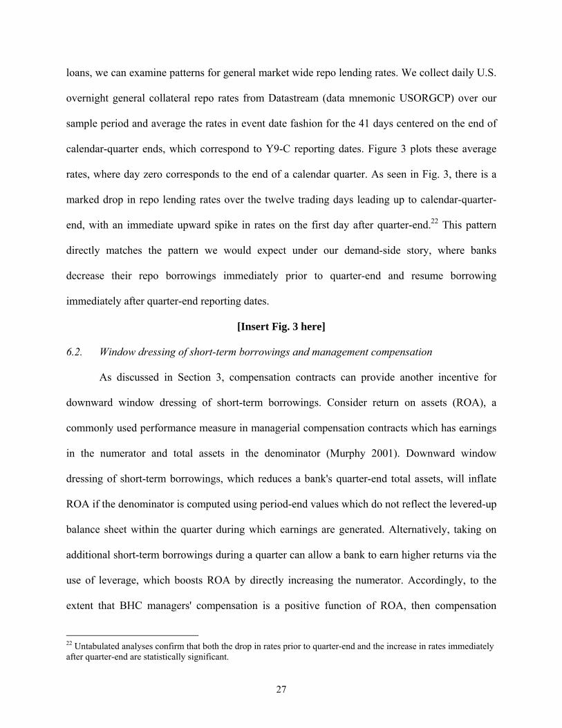
loans, we can examine patterns for general market wide repo lending rates. We collect daily U.S.

overnight general collateral repo rates from Datastream (data mnemonic USORGCP) over our

sample period and average the rates in event date fashion for the 41 days centered on the end of

calendar-quarter ends, which correspond to Y9-C reporting dates. Figure 3 plots these average

rates, where day zero corresponds to the end of a calendar quarter. As seen in Fig. 3, there is a

marked drop in repo lending rates over the twelve trading days leading up to calendar-quarter-

end, with an immediate upward spike in rates on the first day after quarter-end.22 This pattern

directly matches the pattern we would expect under our demand-side story, where banks

decrease their repo borrowings immediately prior to quarter-end and resume borrowing

immediately after quarter-end reporting dates.


6.2. Window dressing of short-term borrowings and management compensation

As discussed in Section 3, compensation contracts can provide another incentive for

downward window dressing of short-term borrowings. Consider return on assets (ROA), a

commonly used performance measure in managerial compensation contracts which has earnings

in the numerator and total assets in the denominator (Murphy 2001). Downward window

dressing of short-term borrowings, which reduces a bank's quarter-end total assets, will inflate

ROA if the denominator is computed using period-end values which do not reflect the levered-up

balance sheet within the quarter during which earnings are generated. Alternatively, taking on

additional short-term borrowings during a quarter can allow a bank to earn higher returns via the

use of leverage, which boosts ROA by directly increasing the numerator. Accordingly, to the

extent that BHC managers' compensation is a positive function of ROA, then compensation

22 Untabulated analyses confirm that both the drop in rates prior to quarter-end and the increase in rates immediately after quarter-end are statistically significant.

28

contracts may provide a direct window dressing incentive aside the incentives discussed earlier.

To precisely determine which performance measures are used in compensation contracts, how

they are computed, and which components of compensation they are tied to, we would need

access to the actual contracts, which we are not privy to. As a second-best solution, we

empirically estimate the strength of the correlation between CEO total compensation and ROA

and link the correlation to quarter-end deviations in short-term borrowings. Our logic is that if

compensation indeed provides downward window dressing incentives, quarter-end deviations in

short-term borrowings will be more pronounced for firms where there exists a relatively high

correlation between measured performance (for example, ROA) and CEO total compensation.

We merge our BHC sample with Execucomp and compute measures of correlation

between CEO total compensation and ROA.23 Specifically, we compute CorrROACompi,m,y as

the correlation between the annual change in firm i's return on assets and the change in the log of

CEO m's total compensation using a minimum of three but no more than five years of data

ending the year immediately prior to the year of quarter t, where total compensation includes

salary and bonus and the value of stock option grants and restricted stock grants (refer to

Appendix C for additional details).

We re-estimate Eqs. (2) and (3) after including CorrROAComp as an additional

explanatory variable. If CEO compensation structure provides window-dressing incentives, we

expect a negative coefficient on CorrROAComp in the OLS model of Eq. (2) and a positive

coefficient on CorrROAComp in the logistic model of Eq. (3). As reported in column (1) of

Table 5, there is indeed a significant negative coefficient of −0.002 (t-statistic of −1.89) on

CorrROAComp in the OLS specification, which suggests greater downward window dressing of

23 Because Execucomp only covers relatively large public firms, our sample size is greatly reduced for this analysis. In particular, for this analysis we have 1,278 BHC-quarter observations across 99 distinct bank holding companies.

29

repo and federal funds liabilities when CEO compensation is more sensitive to ROA. Results

from the logistic model in column (2) provide consistent inferences (coefficient of 0.538 with a t-

statistic of 2.57). That is, a close correlation between ROA and CEO total compensation

increases the probability of observing substantial downward quarter-end deviations in repo and

federal funds liabilities. In total, this evidence is consistent with compensation considerations

providing incentives for downward window dressing of short-term borrowings that are

incremental to the incentives documented in Table 4. It is also noteworthy that the relation

between the concentration of repo and federal funds in the total liability structure and downward

window dressing continues to hold in the Table 5 analysis once compensation incentives are

controlled for.


6.3. Window dressing of short-term borrowings and private debt markets

It is possible that ongoing participation as a borrower in the private debt market gives

banks an incentive to downward window dress short-term borrowings to minimize the likelihood

of financial covenant violation, in accordance with the debt covenant hypothesis (Dichev and

Skinner 2002). To test for evidence of private debt market incentives, we merge our BHC sample

with Dealscan, a comprehensive database of private loan contracts. We define an indicator

variable PrivateDebtBorroweri,t that equals one if firm i is the borrower in a loan contract that

spans the quarter t end date, and equals zero otherwise. From our sample of 8,534 firm-quarter

observations, 604 firm-quarters comprised of 62 distinct BHCs have PrivateDebtBorroweri,t = 1.

We re-estimate Eqs. (2) and (3) after including PrivateDebtBorrower as an additional

explanatory variable. If debt market participation provides downward window-dressing

incentives, we expect a negative coefficient on PrivateDebtBorrower in the OLS model of Eq.

30

(2) and a positive coefficient on PrivateDebtBorrower in the logistic model of Eq. (3). As

reported in column (1) of Table 6, there is indeed a negative but statistically insignificant

coefficient of −0.001 (t-statistic of −1.08) on PrivateDebtBorrower in the OLS specification.

However, there is a significantly positive coefficient on PrivateDebtBorrower in the logistic

specification reported in column (2) (coefficient of 0.261 with a t-statistic of 1.76). Although our

proxy for borrowing in private debt markets is admittedly noisy and we have relatively few

observations where banks are themselves borrowers, the logistic specification provides weak

evidence that borrowing in private debt markets increases the probability of observing large

downward repo and federal funds liability window dressing.


6.4. Stock market reaction to window dressing of short-term borrowings

Under the assumption that some market participants process the information contained

within public Y-9C filings that can be used to infer window dressing, we expect the stock market

reaction to unexpected downward quarter-end deviations in short-term borrowings to reflect the

net effect of several factors. First, downward quarter-end deviations in short-term borrowings

suggests that a firm took on more risk during the quarter than implied by their quarter-end

financial data. This may cause investors to revise upward their risk assessment of the firm

involved, and revise downward their assessment of the same quarter’s earnings performance

upon realizing that a larger asset base was required to produce earnings than previously thought.

Furthermore, if these quarter-end deviations are interpreted as active window dressing by bank

managers in an attempt to mask risk (as our initial tests suggest), investors may revise downward

their assessment of the quality or integrity of management. These factors may lead to negative

31

abnormal stock price reactions to unexpected downward quarter-end deviations in short-term

borrowings.

The public disclosure of a bank's Y-9C is generally the first disclosure of data that would

allow capital market participants to infer whether a bank engaged in window dressing of short-

term borrowings in a particular quarter. To examine the stock market reaction to this disclosure,

we conduct a short window event study surrounding the public release date of bank holding

company Y-9Cs. There exists no publicly available machine readable data that discloses the

publication date of a given Y-9C. However, we can exploit knowledge of the systematic

procedures followed by the Federal Reserve in making these reports public to estimate the

publication date. Our conversations with personnel at the Federal Reserve indicate that Y-9C

filings tend to be clustered immediately before the filing deadline of 40 (45) days for the first

three calendar quarters (fourth calendar quarter) and generally become publicly available two

days later.24 Therefore, we code the Y-9C publication date as 42 (47) calendar days after the

quarter-end date for the first three calendar quarters (fourth calendar quarter) of a year, and

measure stock returns in a five-trading-day window centered on the estimated publication date of

the Y-9C.

We estimate the following model using ordinary least squares to assess the market

reaction to repo and federal funds liability window dressing:

, 0 1 , 2 , 3 , 4 ,

5 , 6 , 7 , 8 ,

, ,

i t i t i t i t i t

QA QA QAi t i t i t i t

i t

CAR RepoFFLiabDEV OtherBorrDEV DepositDEV ROE

Leverage Leverage NLogSize MktToBook

YearFixedEffects

(4)

24 This timing is further supported by documentation on the Fed's National Information Center website. To the extent some Y-9C filings are made public before or after our estimated publication window, our ability to find announcement period stock reactions to our window dressing measure is diminished.

32

where CARi,t is firm i's five-trading-day cumulative abnormal stock return centered on the

estimated publication date of its quarter t Y-9C. To facilitate interpretation of our market

reaction tests, we impose the condition that the estimated quarter t Y-9C publication date is at

least five days after the earnings announcement date for quarter t. We consider six different

measures of daily expected return in our abnormal return calculation: value-weighted market

return, equally-weighted market return, CRSP size decile return, expected return from both a

value-weighted and equally-weighted market model and expected return from a Fama-French

three-factor model (Fama and French, 1993). As discussed below, our inferences are unaltered

across these six different abnormal return proxies.

The variable ΔRepoFFLiabDEVi,t is the change in repo and federal funds liabilities

relative to the prior quarter, where RepoFFLiabDEVi,t-1 proxies for the market’s expectation of

the current quarter’s window dressing activity. We also include analogous measures for deposits

and “other borrowed money.” If investors react more negatively to greater unexpected quarter-

end deviations in repo and federal funds liabilities, we expect 1 > 0. On the other hand, because

quarter-end deviations in deposits or “other borrowed money” is unlikely to be the result of

window dressing, we do not expect to see price reactions to changes in these measures. In

addition, we control for seasonal changes in accounting performance and leverage (ΔROE and

ΔLeverageQA), as well as leverage, size and market-to-book, as these variables may affect firm

stock return. Because the estimated Y-9C publication date occurs after the same quarter’s

earnings announcement, these accounting variables may not elicit price reactions at the release of

the Y-9C filing. We further examine whether there are longer term market effects related to such

window dressing by estimating a variant of Eq. (4) where we replace CARi,t with CARPosti,t,

33

where CARPosti,t is firm i's cumulative abnormal return over the trading-day window [+3, +30]

relative to the estimated quarter t Y-9C publication date.25

Table 7 presents the results of estimating Eq. (4). Column (1) reports results with CAR

computed using value-weighted market returns, and column (2) reports results with CAR

computed using the Fama and French three-factor model (Fama and French, 1993) estimated

using daily returns over the trading day window [45, 6] [+6, +45]. As reported in both

models, there is a significant positive relation between unexpected quarter-end deviations in repo

and federal funds liabilities (ΔRepoFFLiabDEV) and the abnormal return surrounding the

estimated publication date of a BHC's Y-9C (coefficient of 0.180 with a t-statistic of 2.14 and

coefficient of 0.161 with a t-statistic of 2.05 in columns (1) and (2), respectively).26 Because

negative realizations of ΔRepoFFLiabDEVi,t imply greater unexpected downward quarter-end

deviations, this finding reveals that the equity market responds negatively to unexpected

downward quarter-end deviations in short-term borrowings. This finding suggests that at least

some market participants incorporate the information about quarter-end deviations in short-term

borrowings that is revealed in BHC's Y-9C regulatory filings, and that they react in a manner

consistent with negative updating regarding bank performance and risk level during the quarter

and/or management quality/integrity. In untabulated analysis, we estimate Eq. (4) separately for

the top fifty sample and the non-top fifty sample and find consistent inferences across the large

and small BHC subsamples.


25 Given that the publication date of the Y9-C is 42 or 47 calendar days after the end of calendar quarter t, this post window effectively ends at the close of calendar quarter t+1, which by construction is prior to firm i's quarter t+1 earnings announcement date, and therefore avoids confounding effects from the earnings announcement for quarter t+1. 26 Inferences are unaltered if we measure expected returns using equally-weighted market returns, expected returns from a market model estimated using value-weighted or equally-weighted market returns, or CRSP size-decile returns.

34

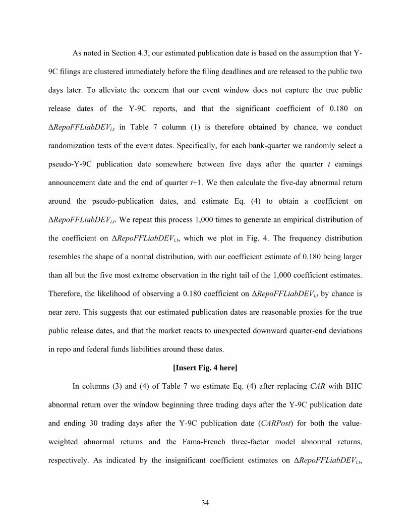
As noted in Section 4.3, our estimated publication date is based on the assumption that Y-

9C filings are clustered immediately before the filing deadlines and are released to the public two

days later. To alleviate the concern that our event window does not capture the true public

release dates of the Y-9C reports, and that the significant coefficient of 0.180 on

ΔRepoFFLiabDEVi,t in Table 7 column (1) is therefore obtained by chance, we conduct

randomization tests of the event dates. Specifically, for each bank-quarter we randomly select a

pseudo-Y-9C publication date somewhere between five days after the quarter t earnings

announcement date and the end of quarter t+1. We then calculate the five-day abnormal return

around the pseudo-publication dates, and estimate Eq. (4) to obtain a coefficient on

ΔRepoFFLiabDEVi,t. We repeat this process 1,000 times to generate an empirical distribution of

the coefficient on ΔRepoFFLiabDEVi,t, which we plot in Fig. 4. The frequency distribution

resembles the shape of a normal distribution, with our coefficient estimate of 0.180 being larger

than all but the five most extreme observation in the right tail of the 1,000 coefficient estimates.

Therefore, the likelihood of observing a 0.180 coefficient on ΔRepoFFLiabDEVi,t by chance is

near zero. This suggests that our estimated publication dates are reasonable proxies for the true

public release dates, and that the market reacts to unexpected downward quarter-end deviations

in repo and federal funds liabilities around these dates.


In columns (3) and (4) of Table 7 we estimate Eq. (4) after replacing CAR with BHC

abnormal return over the window beginning three trading days after the Y-9C publication date

and ending 30 trading days after the Y-9C publication date (CARPost) for both the value-

weighted abnormal returns and the Fama-French three-factor model abnormal returns,

respectively. As indicated by the insignificant coefficient estimates on ΔRepoFFLiabDEVi,t,

35

there is no evidence of under- or overreaction to the Y-9C information concerning quarter-end

deviations from quarterly averages.

Finally, we note that columns (1) and (3) of Table 7 report a significant positive

coefficient on a measure of unexpected earnings (ΔROEi,t), which is somewhat puzzling given

that we ensure via our sample construction procedures that no observations have overlapping

earnings announcement and Y-9C publication date windows. However, the timing of the Y-9C

publication relative to the corresponding quarter t earnings announcement places the Y-9C

window within the period during which extant literature has documented post-earnings-

announcement drift effects (e.g., Ball and Brown, 1968). Therefore, one potential explanation is

that the positive coefficient on ΔROEi,t is an artifact of post-earnings-announcement drift.

6.5. Additional considerations

6.5.1. Trading assets

It is possible that bank management has incentives to systematically reduce holdings of

riskier asset classes at quarter end to project a lower risk profile and to increase its risk-based

capital adequacy ratios. If such asset window dressing occurs, and the assets that are window

dressed are funded by repo and federal funds liabilities, it is possible that observed window

dressing of short-term borrowings is a byproduct of risky asset window dressing. However, with

the current Y-9C disclosures of asset account quarterly averages, it is impossible for us to

empirically examine the existence of window dressing of end-of-quarter holdings of risky assets.

One account where such risky asset window dressing may occur is trading assets. The Y-9C

reports only the quarterly average of total trading assets, not the quarterly averages of the

subcategories of trading assets with different risk levels. With the limited Y-9C data, we do find

that the window dressing measure of total trading assets is not significantly different from zero.

36

Furthermore, short-term borrowing window dressing in repo and federal funds is not associated

with the existence of more risky trading assets at the prior quarter end. Based on this evidence, it

is unlikely that the short-term borrowings window dressing we document is simply a byproduct

of window dressing of risky assets.

6.5.2. Net repo and federal funds

As previously discussed, in addition to being borrowers in the repo and federal funds

markets, bank holding companies can be lenders in these markets, where such transactions create

repo and federal funds assets. Our analysis thus far has not considered whether our sample

banks alter their lending in the repo and federal funds markets around quarter end, because our

descriptive evidence suggests that our sample banks have relatively small repo and federal funds

asset positions. However, for completeness, we repeat our main tests with a measure of net repo

and federal funds liability window dressing, constructed by subtracting repo and federal funds

asset window dressing components from the corresponding liability components. Our inferences

are unaltered when using the net repo and federal funds liability window dressing measure.

6.5.3. Reserve maintenance periods

Banks may use repo and federal funds borrowings to manage their reserve balance

requirements (e.g., Furfine, 2000). A natural question that follows is whether the repo and

federal funds liability window dressing around quarter-end that we document is partially driven

by activities related to reserve maintenance. We do not believe that reserve maintenance affects

our results for several reasons. First, this concern arises only if the end of a bank's reserve

accounting period overlaps with the quarter-end date over which we compute window dressing.

Most large banks are on a weekly reserve calculation and reporting cycle, so there is not a

concentrated incentive related to reserve balances at quarter end. Second, since 1998 reserve

37

requirements are computed on a lagged basis, such that banks clearly know their reserve

requirements well in advance of the end of the maintenance period associated with each weekly

report. Therefore, reserve requirement surprises which would drive an immediate need for

borrowing do not likely exist, in contrast to the dynamics that existed under the reserve

accounting regime prior to 1998. Third, reserve requirements are satisfied based on average

balances over the reserve maintenance period, rather than on period-end balances. Again, this

diminishes the likelihood of concentrated incentives at the end of reserve accounting periods.

Finally, setting the above points aside, if banks indeed use repo and federal funds borrowings to

meet reserve requirements, that would suggest an increase in repo and federal funds borrowings,

and would therefore work against our finding of downward window dressing.

7. Conclusion

This study provides the first empirical evidence on the window dressing of short-term

borrowings through repo and federal funds liability accounts and the stock market’s reaction to

the public release of information that can be used to infer such window dressing. We find

evidence of significant downward window dressing in these accounts by bank holding

companies, resulting in understatements of quarter-end short-term borrowings that appear

material in a substantial fraction of firm-quarter observations, particularly among the largest

bank holding companies.

We find that firms with greater reliance on short-term borrowings in their liability

structure, lower risk-based capital adequacy ratios, and greater management compensation

sensitivity to ROA are more likely to engage in downward window dressing of short-term

borrowings. We provide some evidence that banks that borrow in private debt markets engage in

more downward window dressing of short-term borrowings, and interpret this finding as

38

consistent with incentives to avoid financial covenant violation. Finally, we show that the stock

market reacts negatively to information indicating greater downward window dressing in repo

and federal funds borrowings. However, we do not speak to whether downward window dressing

of repo and federal funds liabilities is on net beneficial or detrimental to the shareholder wealth,

because positive market reactions to the results of such window dressing, including higher

capital adequacy ratio, higher ROA, and lower probability of covenant violations, may have

already been impounded into share prices from earlier management communications regarding

accounting earnings and certain important quarter-end balance sheet items before the release of

the Y-9C.

The potential implications of our findings go beyond bank holding companies and the

financial industry. For firms that currently are not subject to quarterly averages disclosures (i.e.,

non-banks), window dressing is difficult, if not impossible, to detect, potentially giving strong

incentives for such behavior. Our results speak to the new SEC proposed “Short-Term

Borrowing Disclosure” rule. In particular, our market tests suggest that investors of firms that are

not currently subject to quarterly average disclosure requirements will likely find the new

disclosure under the proposed rule useful, although any potential benefits of the new disclosure

will need to be weighed against the costs.

39

REFERENCES

Afonso, G., Kovner, A., Schoar, A., 2011. Stressed not frozen: The fed funds market in the financial crisis. Journal of Finance 66, 1109-1139. Allen, L., Peristiani, S., Saunders, A., 1989. Bank size, collateral, and net purchase behavior in the federal funds market: empirical evidence. Journal of Business 62, 501-515. Allen, L., Saunders, A., 1992. Bank window dressing: theory and evidence. Journal of Banking and Finance 16, 585-623. Ball, R., Brown, P., 1968. An empirical evaluation of accounting income numbers. Journal of Accounting Research 6, 159-178. Barclay, M., Smith, C., 1995. The maturity structure of corporate debt. Journal of Finance 50, 609-631. Benmelech, E., Dvir, E., 2011. Does short-term debt increase vulnerability to crisis? Evidence from the East Asian financial crisis. Working paper, Harvard University and NBER. Board of Governors of the Federal Reserve System, 96th Annual Report, 2009. Brunnermeier, M., Pedersen, L., 2009. Market liquidity and funding liquidity. Review of Financial Studies 22, 2201-2238. Choudhry, M., 2010. The Repo Handbook, 2/e. Butterworth Heinemann. Dechow, P., Shakespeare, C., 2009. Managers time securitization transactions to obtain accounting benefits? The Accounting Review 84, 99-132. Dichev, I., Skinner, D., 2002. Large-sample evidence on the debt covenant hypothesis. Journal of Accounting Research 40, 1092-1123. Fama, E., French, K., 1993. Common risk factors in the returns on stocks and bonds. Journal of Financial Economics 33, 3-56. Feltham, G., Xie, J., 1994. Performance measure congruity and diversity in multi-task principal/agent relations. The Accounting Review 69, 429-453. Furfine, C., 2000. Interbank payments and the daily federal funds rate. Journal of Monetary Economics 46, 535-553. Gorton, G., Metrick, A., 2011. Securitized banking and the run on repo. Journal of Financial Economics, Forthcoming.

40

He, J., Ng, L., Wang, Q., 2004. Quarterly trading patterns of financial institutions. Journal of Business 77, 493-509. He, Z., Xiong, W., 2009. Liquidity and short-term debt crises. Working paper, University of Chicago and NBER. Hördahl, P., King, M., 2008. Developments in repo markets during the financial turmoil. BIS Quarterly Review. Bank for International Settlements. December 2008, 37-53. Kotomin, V., Winters, D., 2006. Quarter-end effects in banks: preferred habitat or window dressing? Journal of Financial Services Research 29, 61-82. Lakonishok, J., Shleifer, A., Thaler, R., Vishny, R., 1991. Window dressing by pension fund managers. American Economic Review (Papers and Proceedings) 81, 227-231. Messier, W., Glover, S., Prawitt, D., 2012. Auditing and Assurance Services: A Systematic Approach, 8/e. McGraw-Hill. Murphy, K., 2001. Performance standards in incentive contracts. Journal of Accounting and Economics 30, 245-278. Musto, D., 1999. Investment decisions depend on portfolio disclosures, Journal of Finance 54, 935-952. Ng, L., Wang, Q., 2004. Institutional trading and the turn-of-the-year effect. Journal of Financial Economics 74, 343-366. Petersen, M., 2009. Estimating standard errors in finance panel data sets: comparing approaches. Review of Financial Studies 22, 435-480. Securities and Exchange Commission, 2010. Short-term borrowing disclosure. Release Nos. 33-9143; 34-62932; File No. S7-22-10. Shleifer, A., Vishny, R., 2010. Unstable banking. Journal of Financial Economics 97, 306-318. Stigum, M., 2007. Stigum's Money Market. New York: McGraw-Hill. Valukas, A., EXAMINER of UNITED STATES BANKRUPTCY COURT SOUTHERN DISTRICT OF NEW YORK, March 2010. “In re LEHMAN BROTHERS HOLDINGS INC., et al., Debtors.” Chapter 11 Case No. 08�13555 (JMP). Warner, J., Wu, J., 2011. Why do mutual fund advisory contracts change? Performance, growth and spillover effects. Journal of Finance, Forthcoming. Whittington, R., Pany, K., 2010. Principles of Auditing & Other Assurance Services, 17/e. McGraw-Hill.

41

Appendix A Disclosure requirements for within-quarter information on balance sheet liability accounts

Authority The Federal Reserve

The SEC Current rule SEC Industry Guide 3

The SEC Proposed rule Release Nos. 33-9143; 34-62932

Apply to Bank Holding Companies Bank Holding Companies All companies that provide MD&A, financial or otherwise

Frequency Quarterly Y-9C, Schedule HC-K Annual 10-K disclosure Quarterly (10-Qs) and Annually (10-Ks)

Financial industry requirements

Averages (daily or weekly basis) of the following accounts-- * Deposits * Federal funds purchased and securities sold under agreements to repurchase * Other borrowed money

Averages (daily or weekly basis) and maximum month-end amounts of the following short-term borrowing accounts-- * Federal funds purchased and securities sold under agreements to repurchase *Commercial paper * Other borrowed money

Averages (daily basis) and maximum daily amounts of the following accounts-- * Federal funds purchased and securities sold under agreements to repurchase *Commercial paper * Borrowings from banks * Borrowings from other financial institutions *Other short-term borrowing

Nonfinancial industry requirements

None None Averages (at the minimum on a monthly basis) and maximum month-end amounts of the above short-term borrowing accounts.

42

Appendix B Variable Definitions Italicized variable names beginning with "BH" in the descriptions refer to the mnemonic data identifiers of raw data items obtained from the Federal Reserve Bank Holding Company data set at http://www.chicagofed.org/webpages/banking/financial_institution_reports/bhc_data.cfm. Referenced "Schedules" are from Form Y-9C. Schedule HC is the "Consolidated Balance Sheet." Schedule HC-B is "Securities." Schedule HC-E is "Deposit Liabilities." Schedule HC-K is "Quarterly Averages." Schedule HC-R is "Regulatory Capital." Schedule HI is the "Consolidated Income Statement."

Cashi,t End of quarter cash and balances due from depository institutions from firm i's quarter t Schedule HC (BHCK0081 + BHCK0395 + BHCK0397).

CorrROACompi,m,y

Correlation between annual change in firm i's return on assets (ROA) and change in the log of CEO m's total compensation, computed using a minimum of three years but no more than five years of data ending in the year immediately prior to the year of quarter t. ROA is computed as net income (Compustat ni) divided by beginning of year total assets (Compustat at). CEO total compensation is Execucomp TDC1.

Debti,t End of quarter debt, including subordinated notes and debentures, from firm i's quarter t Schedule HC (BHCK4062 + BHCKC699).

Depositi,t End of quarter domestic and foreign deposits from firm i's quarter t Schedules HC-E and HC (BHCB3187 + BHCB2389 + BHCB6648 + BHCB2604 + BHOD3187 + BHOD2389 + BHOD6648 + BHOD2604 + BHFN6636).

DepositQAi,t Sum of quarterly average domestic and foreign interest bearing

deposits from firm i's quarter t Schedule HC-K (BHCK3517 + BHCK3404).

DepositDEVi,t Firm i's quarter t quarter-end deviation in deposits, calculated as the average of the beginning and end-of quarter deposits (Deposit) less quarterly average deposits (DepositQA), scaled by quarterly average total assets (TotalAssetQA).

Equityi,t End of quarter total bank holding company equity capital from firm i's quarter t Schedule HC (BHCK3210).

EquityQAi,t Quarterly average total equity capital from firm i's quarter t

Schedule HC-K (BHCK3519).

FamaFrchCARi,t Five-trading-day cumulative abnormal return centered on the estimated date that firm i's quarter t Y-9C report was made public, i.e., trading days [-2, +2]. Abnormal return is computed as firm return less the expected return from a daily Fama-French three-factor model estimated over the [-45, -6] and [+6, +45] trading day windows.

43

FamaFrchCARPosti,t Cumulative abnormal return over the [+3, +30] trading day window relative to the estimated date that firm i's quarter t Y-9C report was made public. Abnormal return is computed as firm return less the expected return from a daily Fama-French three-factor model estimated over the [-45, -6] and [+6, +45] trading day windows.

FixedAsseti,t End of quarter premises and fixed assets from firm i's quarter t Schedule HC (BHCK2145).

GrossLoansi,t End of quarter gross loans, calculated as net loans plus loan loss allowance from firm i's quarter t Schedule HC (BHCKB529 + BHCK3123).

Intangiblei,t End of quarter intangible assets from firm i's quarter t Schedule HC (BHCK3163 + BHCK0426).

LeverageQAi,t TotalAssetQA/EquityQA.

LoanLossResrvei,t Provision for loan losses during firm i's quarter t from Schedule HI (BHCK4230, adjusted to remove amounts from prior calendar year quarters) divided by GrossLoans.

MktToBooki,t

Market-to-book ratio, computed as share price times number of common shares outstanding (|PRC| * SHROUT from the CRSP daily file) as of the Y-9C publication date, divided by book value of equity from the Y-9C (BHCK3210).

NLogSizeQAi,t Natural logarithm of TotalAssetQA.

OtherAsseti,t End of quarter "other assets" from firm i's quarter t Schedule HC (BHCK2160).

OtherBorri,t End of quarter "other borrowed money" from firm i's quarter t Schedule HC (BHCK3190).

OtherBorrQAi,t Quarterly average "all other borrowed funds" (including

commercial paper, other short-term borrowed money, and other long-term borrowed money) from firm i's quarter t Schedule HC-K (BHCK2635).

OtherBorrDEVi,t Firm i's quarter t quarter-end deviation in other borrowed money, calculated as the average of the beginning and end-of quarter other borrowed money (OtherBorr) less quarterly average other borrowed money (OtherBorrQA), scaled by quarterly average total assets (TotalAssetQA).

OtherLiabi,t End of quarter "other liabilities" from firm i's quarter t Schedule HC (BHCK2750).

PrivateDebtBorroweri,t An indicator that = 1 if firm i is the borrower in a private loan contract (as reported in LPC's Dealscan) that spans the quarter t end date, and = 0 otherwise.

RepoFFAsseti,t End of quarter federal funds sold and securities purchased under agreements to resell from firm i's quarter t Schedule HC (BHDMB987 + BHCKB989).

44

RepoFFAssetQAi,t Quarterly average federal funds sold and securities purchased

under agreements to resell from firm i's quarter t Schedule HC-K (BHCK3365).

RepoFFAssetDEVi,t Firm i's quarter t quarter-end deviation in federal funds sold and securities purchased under agreements to resell; calculated as the average of the beginning and end-of quarter repo and federal funds assets (RepoFFAsset) less the quarterly average repo and federal funds assets (RepoFFAssetQA), scaled by quarterly average total assets (TotalAssetQA).

RepoFFLiabi,t End of quarter federal funds purchased and securities sold under agreements to repurchase from firm i's quarter t Schedule HC (BHDMB993 + BHCKB995).

RepoFFLiabQAi,t Quarterly average federal funds purchased and securities sold

under agreements to repurchase from firm i's quarter t Schedule HC-K (BHCK3353).

RepoFFLiabBigDownDEVi,t An indicator that =1 if RepoFFLiabDEVi,t is in the most negative sample quartile, and = 0 otherwise.

RepoFFLiabDEVi,t Firm i's quarter t quarter-end deviation in federal funds purchased and securities sold under agreements to repurchase; calculated as the average of the beginning and end-of quarter repo and federal funds liabilities (RepoFFLiab) less the quarterly average repo and federal funds liabilities (RepoFFLiabQA), scaled by quarterly average total assets (TotalAssetQA).

RepoFFToTotalLiabQAi,t Percentage of total liabilities represented by repo and federal

funds liabilities, computed as RepoFFLiabQA/TotalLiabQA.

RepoToRepoFFAsseti,t Percentage of repo and federal funds assets represented by securities purchased under agreements to resell; computed as BHCKB989/RepoFFAsset.

RepoToRepoFFLiabi,t Percentage of repo and federal funds liabilities represented by securities sold under agreements to repurchase; computed as BHCKB995/RepoFFLiab.

ROEi,t Return on equity during firm i's quarter t, computed as net income (BHCK4340, adjusted to remove amounts from prior calendar year quarters) divided by quarterly average equity (EquityQA).

Securitiesi,t End of quarter held-to-maturity plus available-for-sale securities from firm i's quarter t Schedules HC and HC-B (BHCK1754 + BHCK1172).

Tier1Capitali,t

Tier 1 risk-based capital ratio from firm i's quarter t schedule HC-R (BHCK7206).

TotalAsseti,t End of quarter total consolidated assets from firm i's quarter t Schedule HC (BHCK2170).

TotalAssetQAi,t Quarterly average total consolidated assets from firm i's quarter t

Schedule HC-K (BHCK3368).

45

TotalAssetDEVi,t Firm i's quarter t quarter-end deviation in total assets, calculated as the average of the beginning and end-of quarter total assets (TotalAsset) less quarterly average total assets (TotalAssetQA), scaled by quarterly average total assets (TotalAssetQA).

TotalLiabi,t End of quarter assets less end of quarter equity (TA - EQ).

TotalLiabQAi,t Quarterly average assets less quarterly average equity (HCK_TA -

HCK_EQ).

TotalLiabDEVi,t Firm i's quarter t quarter-end deviation in total liabilities, calculated as the average of the beginning and end-of quarter total liabilities (TotalLiab) less quarterly average total liabilities (TotalLiabQA), scaled by quarterly average total assets (TotalAssetQA).

TradingAsseti,t End of quarter trading assets from firm i's quarter t Schedule HC (BHCK3545).

TradingAssetQAi,t Quarterly average trading assets from firm i's quarter t Schedule

HC-K (BHCK3401).

TradingAssetDEVi,t Firm i's quarter t quarter-end deviation in trading assets, calculated as the average of the beginning and end-of quarter trading assets (TradingAsset) less quarterly average trading assets (TradingAssetQA), scaled by quarterly average total assets (TotalAssetQA).

ValueWeightCARi,t Five-trading-day cumulative abnormal return centered on the estimated date that firm i's quarter t Y-9C report was made public, i.e., trading days [-2, +2]. Abnormal return is computed as firm return less CRSP value-weighted market return.

ValueWeightCARPosti,t Cumulative abnormal return over the [+3, +30] trading day window relative to the estimated date that firm i's quarter t Y-9C report was made public. Abnormal return is computed as firm return less CRSP value-weighted market return.

46

Figure 1 Illustration of repo and federal funds liability quarter-end deviation measure Figure 1 provides illustrations of scenarios that would result in quarter-end deviation measure reflecting no deviation (RepoFFLiabDEV = 0) and a downward deviation (RepoFFLiabDEV < 0), respectively, where RepoFFLiabDEV is computed as in Eq. (1).

RepoFFLiab

Quarter-end t-1

Quarter-end t

Downward Quarter-end Deviation

RepoFFLiabDEV < 0

TIME

TIME

RepoFFLiab

Quarter-end t-1

Quarter-end t

No Quarter-end Deviation RepoFFLiabDEV = 0

47

‐0.007

‐0.006

‐0.005

‐0.004

‐0.003

‐0.002

‐0.001

0

0.001

0.002

200206

200209

200212

200303

200306

200309

200312

200403

200406

200409

200412

200503

200506

200509

200512

200603

200606

200609

200612

200703

200706

200709

200712

200803

200806

200809

200812

200903

200906

200909

200912

201003

Top 50 BHCs Non‐Top 50 BHCs

Figure 2 Quarter-end deviations from quarterly averages in repo and federal funds liabilities Figure 2 presents the quarterly sample mean values of RepoFFLiabDEV (i.e., quarter-end deviations in repo and federal funds liabilities), as defined in Appendix B, separately for large (top 50) and small (non-top 50) bank holding company observations each quarter based on total consolidated assets.

48

2.00

2.05

2.10

2.15

2.20

2.25

2.30

2.35

2.40

2.45

2.50

‐20 ‐18 ‐16 ‐14 ‐12 ‐10 ‐8 ‐6 ‐4 ‐2 0 2 4 6 8 10 12 14 16 18 20

U.S. O

vernight GC Repo Lending Rate %

Event Day (Day 0 = calendar quarter end)

Figure 3 Event-time plot of U.S. Overnight General Collateral Repo lending rates Figure 3 presents average event-time daily U.S. overnight general collateral repo lending rates over the period 2001-2010, where day zero corresponds to the last trading day of a calendar quarter.

49

0

5

10

15

20

25

30

35

‐0.3

‐0.285

‐0.27

‐0.255

‐0.24

‐0.225

‐0.21

‐0.195

‐0.18

‐0.165

‐0.15

‐0.135

‐0.12

‐0.105

‐0.09

‐0.075

‐0.06

‐0.045

‐0.03

‐0.015 0

0.015

0.03

0.045

0.06

0.075

0.09

0.105

0.12

0.135

0.15

0.165

0.18

0.195

0.21

0.225

0.24

More

Frequency

Bin

ΔRepoFFLiabDEVcoefficient estimate (0.180) from actual sample estimation of Eq. (4)

Figure 4 Empirical distribution of randomization-based coefficients on unexpected downward quarter-end deviations in repo and federal funds liabilities in the market test Figure 4 presents the empirical distribution of the estimated coefficients on ΔRepoFFLiabDEV obtained by 1,000 iterations of estimating Eq. (4) where the abnormal return dependent variable is computed based on randomly assigned Y-9C publication dates between the quarter's earnings announcement window and the end of the calendar quarter. Figure 4 also highlights the coefficient estimate on ΔRepoFFLiabDEV (0.180) obtained by estimating Eq. (4) using our coded Y-9C publication date of 42 (47) days after the "as-of" date for the first three (last) calendar quarters, as reported in Table 7 column (1).

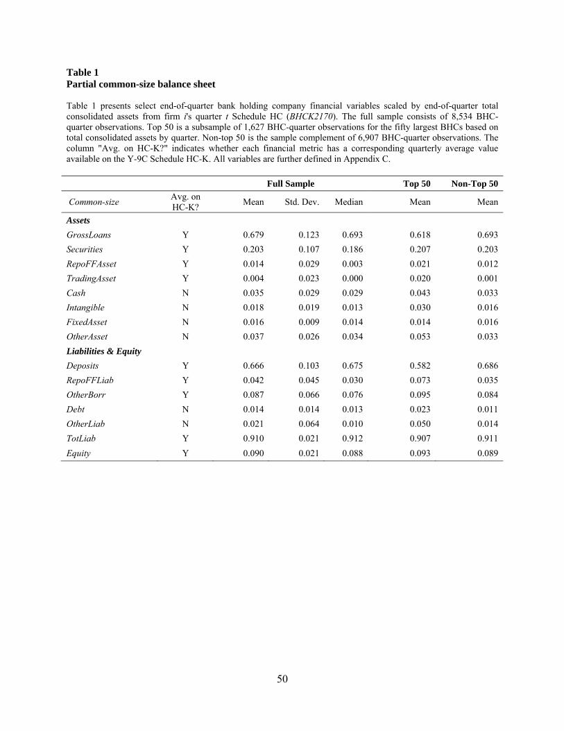
50

Table 1 Partial common-size balance sheet Table 1 presents select end-of-quarter bank holding company financial variables scaled by end-of-quarter total consolidated assets from firm i's quarter t Schedule HC (BHCK2170). The full sample consists of 8,534 BHC-quarter observations. Top 50 is a subsample of 1,627 BHC-quarter observations for the fifty largest BHCs based on total consolidated assets by quarter. Non-top 50 is the sample complement of 6,907 BHC-quarter observations. The column "Avg. on HC-K?" indicates whether each financial metric has a corresponding quarterly average value available on the Y-9C Schedule HC-K. All variables are further defined in Appendix C.

Full Sample Top 50 Non-Top 50

Common-size Avg. on HC-K?

Mean Std. Dev. Median Mean Mean

Assets

GrossLoans Y 0.679 0.123 0.693 0.618 0.693

Securities Y 0.203 0.107 0.186 0.207 0.203

RepoFFAsset Y 0.014 0.029 0.003 0.021 0.012

TradingAsset Y 0.004 0.023 0.000 0.020 0.001

Cash N 0.035 0.029 0.029 0.043 0.033

Intangible N 0.018 0.019 0.013 0.030 0.016

FixedAsset N 0.016 0.009 0.014 0.014 0.016

OtherAsset N 0.037 0.026 0.034 0.053 0.033

Liabilities & Equity

Deposits Y 0.666 0.103 0.675 0.582 0.686

RepoFFLiab Y 0.042 0.045 0.030 0.073 0.035

OtherBorr Y 0.087 0.066 0.076 0.095 0.084

Debt N 0.014 0.014 0.013 0.023 0.011

OtherLiab N 0.021 0.064 0.010 0.050 0.014

TotLiab Y 0.910 0.021 0.912 0.907 0.911

Equity Y 0.090 0.021 0.088 0.093 0.089

51

Table 2 Sample descriptive statistics Table 2 presents sample descriptive statistics for firm-quarter variables used in our analyses. All variables are defined in Appendix C. *, **, and *** indicate that the mean is significantly different from zero at the 10%, 5%, and 1% levels, respectively. Top 50 is a subsample of BHC-quarter observations for the fifty largest BHCs based on total consolidated assets by quarter. Non-top 50 is the sample complement of relatively small BHCs.

Full Sample Top 50 Non-Top 50

Variable N Mean Std P25 Median P75 Mean Mean

RepoFFToTotLiabQA 8,534 0.0477 *** 0.0501 0.0082 0.0342 0.0702 0.0853 *** 0.0389 ***

RepoFFLiabDEV 8,534 -0.0009 *** 0.0072 -0.0024 0.0000 0.0015 -0.0035 *** -0.0003 ***

DepositDEV 8,534 0.0331 *** 0.0524 -0.0028 0.0105 0.0690 0.0444 *** 0.0304 ***

OtherBorrDEV 8,534 -0.0022 *** 0.0112 -0.0063 0.0000 0.0026 -0.0024 *** -0.0022 ***

RepoFFAssetDEV 8,462 -0.0004 *** 0.0076 -0.0020 0.0000 0.0014 -0.0003 *** -0.0004 ***

TradingAssetDEV 8,287 -0.0000 0.0006 0.0000 0.0000 0.0000 -0.0000 -0.0000

TotalAssetDEV 8,459 0.0040 *** 0.0154 -0.0021 0.0040 0.0106 0.0039 *** 0.0040 ***

TotalLiabDEV 8,462 0.0042 *** 0.0152 -0.0018 0.0042 0.0107 0.0040 *** 0.0042 ***

LeverageQAt-1 8,534 11.6040 *** 2.5654 9.8930 11.3240 13.0673 11.2537 *** 11.6865 ***

Tier1Capitalt-1 8,531 11.4683 *** 2.5646 9.8600 11.0300 12.5800 10.2774 *** 11.7483 ***

NLogSizet-1 8,534 14.8867 *** 1.5735 13.7387 14.4924 15.5525 17.4928 *** 14.2729 ***

LoanLossResrvet-1 8,534 0.0017 *** 0.0027 0.0004 0.0008 0.0016 0.0024 *** 0.0015 ***

RepoToRepoFFAsset 5,792 0.1466 *** 0.3204 0.0000 0.0000 0.0000 0.4354 *** 0.0543 ***

RepoToRepoFFLiab 7,140 0.7799 *** 0.3087 0.6383 0.9600 1.0000 0.7009 *** 0.8027 ***

ValueWeightCAR 8,461 0.0002 0.0434 -0.0207 -0.0018 0.0197 -0.0038 *** 0.0012 **

FamaFrchCAR 8,408 0.0042 *** 0.0531 -0.0178 0.0015 0.0231 0.0038 *** 0.0043 ***

ΔRepoFFLiabDEV 8,150 0.0000 0.0072 -0.0023 0.0000 0.0024 0.0001 -0.0000

ΔROE 8,194 -0.0050 *** 0.0296 -0.0080 -0.0018 0.0025 -0.0052 *** -0.0050 ***

ΔLeverageQA 8,531 -0.0158 * 0.8310 -0.2411 -0.0048 0.2312 -0.0590 *** -0.0056 ***

ΔDepositDEV 8,440 0.0005 0.0290 -0.0078 0.0004 0.0086 0.0008 0.0004

ΔOtherBorrDEV 8,390 -0.0000 0.0106 -0.0040 0.0000 0.0039 -0.0002 0.0000

ROE 8,467 0.0241 *** 0.0314 0.0186 0.0297 0.0379 0.0261 *** 0.0236 ***

MktToBook 8,534 1.7595 *** 0.9361 1.2084 1.7241 2.2063 1.8620 *** 1.7353 ***

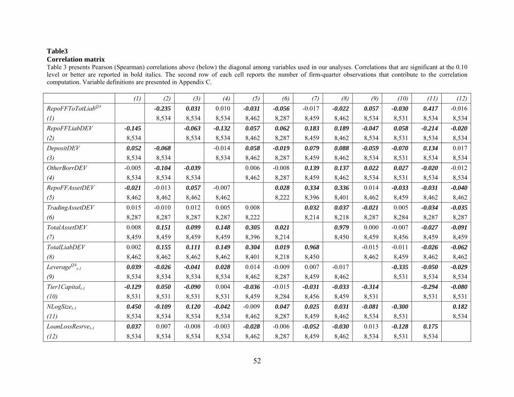
52

Table3 Correlation matrix Table 3 presents Pearson (Spearman) correlations above (below) the diagonal among variables used in our analyses. Correlations that are significant at the 0.10 level or better are reported in bold italics. The second row of each cell reports the number of firm-quarter observations that contribute to the correlation computation. Variable definitions are presented in Appendix C. (1) (2) (3) (4) (5) (6) (7) (8) (9) (10) (11) (12)

RepoFFToTotLiabQA -0.235 0.031 0.010 -0.031 -0.056 -0.017 -0.022 0.057 -0.030 0.417 -0.016

(1) 8,534 8,534 8,534 8,462 8,287 8,459 8,462 8,534 8,531 8,534 8,534

RepoFFLiabDEV -0.145 -0.063 -0.132 0.057 0.062 0.183 0.189 -0.047 0.058 -0.214 -0.020

(2) 8,534 8,534 8,534 8,462 8,287 8,459 8,462 8,534 8,531 8,534 8,534

DepositDEV 0.052 -0.068 -0.014 0.058 -0.019 0.079 0.088 -0.059 -0.070 0.134 0.017

(3) 8,534 8,534 8,534 8,462 8,287 8,459 8,462 8,534 8,531 8,534 8,534

OtherBorrDEV -0.005 -0.104 -0.039 0.006 -0.008 0.139 0.137 0.022 0.027 -0.020 -0.012

(4) 8,534 8,534 8,534 8,462 8,287 8,459 8,462 8,534 8,531 8,534 8,534

RepoFFAssetDEV -0.021 -0.013 0.057 -0.007 0.028 0.334 0.336 0.014 -0.033 -0.031 -0.040

(5) 8,462 8,462 8,462 8,462 8,222 8,396 8,401 8,462 8,459 8,462 8,462

TradingAssetDEV 0.015 -0.010 0.012 0.005 0.008 0.032 0.037 -0.021 0.005 -0.034 -0.035

(6) 8,287 8,287 8,287 8,287 8,222 8,214 8,218 8,287 8,284 8,287 8,287

TotalAssetDEV 0.008 0.151 0.099 0.148 0.305 0.021 0.979 0.000 -0.007 -0.027 -0.091

(7) 8,459 8,459 8,459 8,459 8,396 8,214 8,450 8,459 8,456 8,459 8,459

TotalLiabDEV 0.002 0.155 0.111 0.149 0.304 0.019 0.968 -0.015 -0.011 -0.026 -0.062

(8) 8,462 8,462 8,462 8,462 8,401 8,218 8,450 8,462 8,459 8,462 8,462

LeverageQAt-1 0.039 -0.026 -0.041 0.028 0.014 -0.009 0.007 -0.017 -0.335 -0.050 -0.029

(9) 8,534 8,534 8,534 8,534 8,462 8,287 8,459 8,462 8,531 8,534 8,534

Tier1Capitalt-1 -0.129 0.050 -0.090 0.004 -0.036 -0.015 -0.031 -0.033 -0.314 -0.294 -0.080

(10) 8,531 8,531 8,531 8,531 8,459 8,284 8,456 8,459 8,531 8,531 8,531

NLogSizet-1 0.450 -0.109 0.120 -0.042 -0.009 0.047 0.025 0.031 -0.081 -0.300 0.182

(11) 8,534 8,534 8,534 8,534 8,462 8,287 8,459 8,462 8,534 8,531 8,534

LoanLossResrvet-1 0.037 0.007 -0.008 -0.003 -0.028 -0.006 -0.052 -0.030 0.013 -0.128 0.175

(12) 8,534 8,534 8,534 8,534 8,462 8,287 8,459 8,462 8,534 8,531 8,534

53

Table 4 Window dressing of repo and federal funds liabilities and risk-based incentives Table 4 presents results from OLS regression of quarter-end deviations in short-term borrowings on a set of bank-quarter determinants using a sample of publicly traded bank holding companies. Columns (1), (2) and (3) are estimated using ordinary least squares, and Columns (4), (5) and (6) are estimated using logistic regression. Columns (1) and (4) are estimated using the full sample. Columns (2) and (5) are estimated using the fifty largest banks each quarter based on consolidated total assets. Columns (3) and (6) are estimated using the sample complement of relatively small banks. RepoFFLiabDEV is the continuous measure of quarter-end deviation in repo and fed funds liabilities. RepoFFLiabBigDownDEV is an indicator variables = 1 if RepoFFLiabDEV is in the most negative sample quartile (which indicates a high magnitude of downward quarter-end deviation), and = 0 otherwise. All variables are further defined in Appendix C. Robust t-statistics based on two-way clustered standard errors at the bank and calendar quarter-year levels are reported in parentheses. *, **, and *** indicate significance (two-sided) at the 10%, 5%, and 1% levels. R2 refers to adjusted-R2 in Columns (1), (2) and (3) and pseudo-R2 in Columns (4), (5) and (6). Dep. Var.: RepoFFLiabDEV RepoFFLiabBigDownDEV Sample: Full Top 50 Non-Top 50 Full Top 50 Non-Top 50 Column: Pred. Sign (1) (2) (3) Pred. Sign (4) (5) (6) Intercept 0.0120*** 0.0165 0.0033 -3.8951*** -1.6959 -3.0495** (3.37) (1.54) (1.08) (-4.27) (-0.80) (-2.44) RepoFFToTotLiabQA -0.0243*** -0.0387*** -0.0208*** + 12.8826*** 8.6729*** 15.3583*** (-5.17) (-3.82) (-4.14) (9.38) (4.94) (7.97) Tier1Capitalt-1 + -0.0000 0.0004*** -0.0001 -0.0484** -0.1646*** -0.0173 (-0.22) (2.63) (-1.53) (-2.21) (-3.65) (-0.75) DepositDEV -0.0059* -0.0192* -0.0025 1.2465 4.1706** -0.0852 (-1.91) (-1.89) (-1.08) (1.36) (2.14) (-0.09) OtherBorrDEV -0.0862*** -0.1238*** -0.0710*** 18.9591*** 27.6575*** 16.2172*** (-6.26) (-3.45) (-5.02) (5.06) (3.78) (3.54) NLogSizet-1 -0.0006*** -0.0009 -0.0000 0.1561*** 0.1296 0.0480 (-3.18) (-1.62) (-0.13) (3.37) (1.17) (0.63) LeverageQA

t-1 -0.0001* -0.0003 -0.0001 0.0122 -0.0134 0.0291 (-1.90) (-1.51) (-1.15) (0.52) (-0.25) (1.14) LoanLossResrvet-1 -0.0754* -0.2964** -0.0338 3.5336 52.3050 -8.0274 (-1.65) (-2.26) (-1.05) (0.18) (1.27) (-0.41) Fixed Effects Year Year Year Year Year Year N 8,531 1,624 6,907 8,531 1,624 6,907 R2 0.095 0.171 0.042 0.121 0.124 0.093

54

Table 5 Window dressing of repo and federal funds liabilities and management compensation Table 5 presents results from OLS regression of quarter-end deviations in short-term borrowings on a set of bank-quarter determinants using a sample of publicly traded bank holding companies. Column (1) is estimated using ordinary least squares, and Column (2) is estimated using logistic regression. RepoFFLiabDEV is the continuous measure of quarter-end deviation in repo and fed funds liabilities. RepoFFLiabBigDownnDEV is an indicator variables = 1 if RepoFFLiabDEV is in the most negative sample quartile (which indicates a high magnitude of downward quarter-end deviation), and = 0 otherwise. CorrROAComp is the sensitivity of CEO total compensation to return on assets, measured as the correlation between the annual change in ROA and the annual change in log total compensation. All variables are further defined in Appendix C. Robust t-statistics based on two-way clustered standard errors at the bank and calendar quarter-year levels are reported in parentheses. *, **, and *** indicate significance (two-sided) at the 10%, 5%, and 1% levels, respectively. R2 refers to adjusted-R2 in Column (1) and pseudo-R2 in Column (2). Dep. Var.: RepoFFLiabDEV RepoFFLiabBigDownDEV Column: Pred. Sign (1) Pred. Sign (2) Intercept 0.0198* -3.3814* (1.95) (-1.80) CorrROAComp -0.0020* + 0.5376**

(-1.89) (2.57) RepoFFToTotLiabQA -0.0266*** + 5.3841*** (-2.77) (3.53) Tier1Capitalt-1 + 0.0002 -0.1224*** (1.20) (-3.30) DepositDEV -0.0122 1.7945 (-1.23) (0.87) OtherBorrDEV -0.1128*** 25.1110*** (-2.72) (3.54) NLogSizet-1 -0.0012** 0.2425** (-2.08) (2.26) LeverageQA

t-1 -0.0001 -0.0246 (-0.86) (-0.58) LoanLossResrvet-1 -0.1259 -39.0772 (-1.04) (-0.91) Fixed Effects Year Year N 1,207 1,207 R2 0.147 0.117

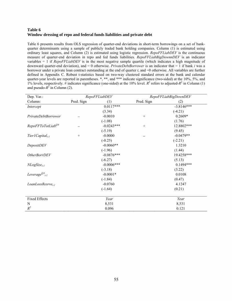
55

Table 6 Window dressing of repo and federal funds liabilities and private debt Table 6 presents results from OLS regression of quarter-end deviations in short-term borrowings on a set of bank-quarter determinants using a sample of publicly traded bank holding companies. Column (1) is estimated using ordinary least squares, and Column (2) is estimated using logistic regression. RepoFFLiabDEV is the continuous measure of quarter-end deviation in repo and fed funds liabilities. RepoFFLiabBigDownnDEV is an indicator variables = 1 if RepoFFLiabDEV is in the most negative sample quartile (which indicates a high magnitude of downward quarter-end deviation), and = 0 otherwise. PrivateDebtBorrower is an indicator that = 1 if bank i was a borrower under a private loan contract outstanding at the end of quarter t, and =0 otherwise. All variables are further defined in Appendix C. Robust t-statistics based on two-way clustered standard errors at the bank and calendar quarter-year levels are reported in parentheses. *, **, and *** indicate significance (two-sided) at the 10%, 5%, and 1% levels, respectively. # indicates significance (one-sided) at the 10% level. R2 refers to adjusted-R2 in Column (1) and pseudo-R2 in Column (2). Dep. Var.: RepoFFLiabDEV RepoFFLiabBigDownDEV Column: Pred. Sign (1) Pred. Sign (2) Intercept 0.0117*** -3.8146*** (3.34) (-4.21) PrivateDebtBorrower -0.0010 + 0.2609* (-1.08) (1.76) RepoFFToTotLiabQA -0.0243*** + 12.8802*** (-5.19) (9.45) Tier1Capitalt-1 + -0.0000 -0.0479** (-0.25) (-2.21) DepositDEV -0.0060** 1.3210 (-1.96) (1.44) OtherBorrDEV -0.0876*** 19.4258*** (-6.27) (5.13) NLogSizet-1 -0.0006*** 0.1494*** (-3.18) (3.22) LeverageQA

t-1 -0.0001* 0.0108 (-1.84) (0.47) LoanLossResrvet-1 -0.0760 4.1247 (-1.64) (0.21) Fixed Effects Year Year N 8,531 8,531 R2 0.096 0.121

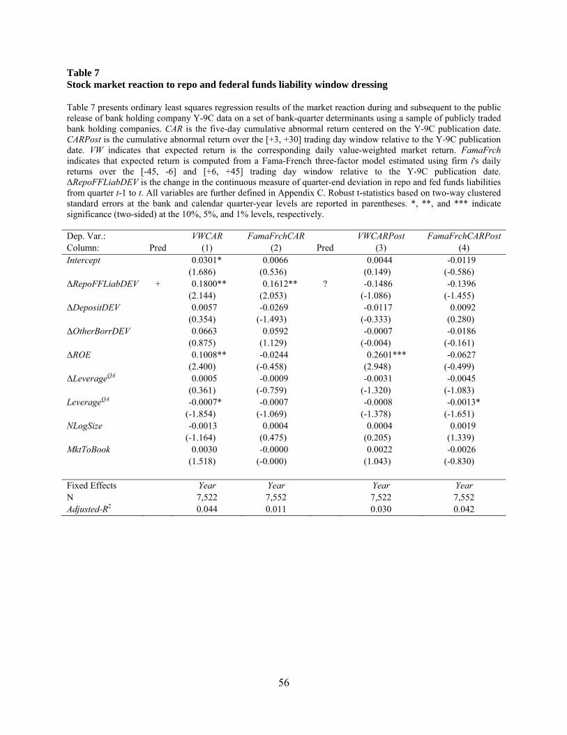
56

Table 7 Stock market reaction to repo and federal funds liability window dressing Table 7 presents ordinary least squares regression results of the market reaction during and subsequent to the public release of bank holding company Y-9C data on a set of bank-quarter determinants using a sample of publicly traded bank holding companies. CAR is the five-day cumulative abnormal return centered on the Y-9C publication date. CARPost is the cumulative abnormal return over the [+3, +30] trading day window relative to the Y-9C publication date. VW indicates that expected return is the corresponding daily value-weighted market return. FamaFrch indicates that expected return is computed from a Fama-French three-factor model estimated using firm i's daily returns over the [-45, -6] and [+6, +45] trading day window relative to the Y-9C publication date. ΔRepoFFLiabDEV is the change in the continuous measure of quarter-end deviation in repo and fed funds liabilities from quarter t-1 to t. All variables are further defined in Appendix C. Robust t-statistics based on two-way clustered standard errors at the bank and calendar quarter-year levels are reported in parentheses. *, **, and *** indicate significance (two-sided) at the 10%, 5%, and 1% levels, respectively. Dep. Var.: VWCAR FamaFrchCAR VWCARPost FamaFrchCARPost Column: Pred (1) (2) Pred (3) (4) Intercept 0.0301* 0.0066 0.0044 -0.0119 (1.686) (0.536) (0.149) (-0.586) ΔRepoFFLiabDEV + 0.1800** 0.1612** ? -0.1486 -0.1396 (2.144) (2.053) (-1.086) (-1.455) ΔDepositDEV 0.0057 -0.0269 -0.0117 0.0092 (0.354) (-1.493) (-0.333) (0.280) ΔOtherBorrDEV 0.0663 0.0592 -0.0007 -0.0186 (0.875) (1.129) (-0.004) (-0.161) ΔROE 0.1008** -0.0244 0.2601*** -0.0627 (2.400) (-0.458) (2.948) (-0.499) ΔLeverageQA 0.0005 -0.0009 -0.0031 -0.0045 (0.361) (-0.759) (-1.320) (-1.083) LeverageQA -0.0007* -0.0007 -0.0008 -0.0013* (-1.854) (-1.069) (-1.378) (-1.651) NLogSize -0.0013 0.0004 0.0004 0.0019 (-1.164) (0.475) (0.205) (1.339) MktToBook 0.0030 -0.0000 0.0022 -0.0026 (1.518) (-0.000) (1.043) (-0.830) Fixed Effects Year Year Year Year N 7,522 7,552 7,522 7,552 Adjusted-R2 0.044 0.011 0.030 0.042

Window Dressing of Short-Term Borrowingsutah-wac.org/2012/Papers/owens_UWAC.pdf · 2012-02-15 ·...

Documents

Transcript of Window Dressing of Short-Term Borrowingsutah-wac.org/2012/Papers/owens_UWAC.pdf · 2012-02-15 ·...