Wind-Wave Probabilistic Forecasting based on Ensemble ... · Summary Wind and wave forecasts are of...
101
Wind-Wave Probabilistic Forecasting based on Ensemble Predictions Maxime FORTIN Kongens Lyngby 2012 IMM-MSc-2012-86
Transcript of Wind-Wave Probabilistic Forecasting based on Ensemble ... · Summary Wind and wave forecasts are of...

Wind-Wave ProbabilisticForecasting based on Ensemble
Predictions
Maxime FORTIN
Kongens Lyngby 2012
IMM-MSc-2012-86

Technical University of Denmark
Informatics and Mathematical Modelling
Building 321, DK-2800 Kongens Lyngby, Denmark
Phone +45 45253351, Fax +45 45882673
www.imm.dtu.dk IMM-PhD-2012-86

Summary
Wind and wave forecasts are of a crucial importance for a number of decision-making problems. Nowadays, considering all potential uncertainty sources inweather prediction, ensemble forecasting provides the most complete informa-tion about future weather conditions. However, ensemble forecasts tend to bebiased and underdispersive, and are therefore uncalibrated. Calibration meth-ods were developed to solve this issue. So far, these methods are usually appliedon univariate weather forecasts and do not take any possible correlation into ac-count. Since wind and wave forecasts have to be jointly taken into accountin some decision-making problems, e.g. offshore wind farm maintenance, wepropose in this thesis a bivariate approach, generalizing existing univariate cali-bration methods to jointly calibrated ensemble forecasts. A other method usingthe EPS-prescribed correlation in order to recover the dependence lost duringthe marginal calibration is also proposed. Even if the univariate performance ofthe marginal calibration is preserved, results confirm the need for bivariate ap-proaches. Contrary to the univariate approach, the bivariate calibration methodgenerates correlated bivariate forecasts, though it appears to be too sensitiveto outliers when estimating necessary model parameters. Jointly calibrated dis-tributions are too wide and therefore overdispersive. The different calibrationmethods are tested on ECMWF ensemble predictions over the offshore platformFINO1 located in the North Sea close to the German shore.

ii

Preface
This thesis was prepared at the department of Informatics and MathematicalModelling at the Technical University of Denmark in fulfilment of the require-ments for acquiring an M.Sc. in Informatics. My supervisors are Pierre Pinsonand Henrik Madsen from the IMM department at DTU.
The thesis deals with wind and wave ensemble forecast calibration. A univariatecalibration method is employed and the use of a bivariate approach is investi-gated. The different methods are tested on the ECMWF ensemble forecastsover the offshore measurement platforms FINO1 located in the North Sea.
Lyngby, 03-August-2012
Maxime FORTIN

iv

Acknowledgements
This project wouldn’t have been possible without my supervisor Pierre Pinsonthat I sincerely would first like to thank for his ongoing support and the timehe took to help me when needed. Working with him has been a great pleasureand of an enormous interest.
I would also like to thank Henrik Madsen for having permitted me to workamong his group at DTU IMM.
Finally, I am grateful to everyone of the department of statistics of DTU Infor-matics for the ideas they suggested me and their warm welcome.

vi

Contents
Summary i
Preface iii
Acknowledgements v
1 Introduction 1
1.1 What’s the point in forecasting? . . . . . . . . . . . . . . . . . . 2
1.2 Ensemble forecasting . . . . . . . . . . . . . . . . . . . . . . . . . 3
1.3 Ensemble Forecast Verification and Calibration . . . . . . . . . . 6
1.4 Structure . . . . . . . . . . . . . . . . . . . . . . . . . . . . . . . 8
2 Data 9
2.1 Observations . . . . . . . . . . . . . . . . . . . . . . . . . . . . . 11
2.1.1 10 m Wind Speed . . . . . . . . . . . . . . . . . . . . . . 11
2.1.2 Significant Wave Height . . . . . . . . . . . . . . . . . . . 14
2.1.3 Wind and Wave Interaction . . . . . . . . . . . . . . . . . 16
2.1.4 Availability . . . . . . . . . . . . . . . . . . . . . . . . . . 17
2.2 Forecasts . . . . . . . . . . . . . . . . . . . . . . . . . . . . . . . 18
2.2.1 Generalities about wind and wave forecasting . . . . . . . 18
2.2.2 Ensemble forecasting . . . . . . . . . . . . . . . . . . . . . 20
3 Ensemble Forecast verification 23
3.1 Univariate Forecasts Verification . . . . . . . . . . . . . . . . . . 24
3.2 Multivariate Forecasts Verification . . . . . . . . . . . . . . . . . 31
3.3 Skill Score . . . . . . . . . . . . . . . . . . . . . . . . . . . . . . . 35

viii CONTENTS
4 Ensemble Forecast Calibration Method 374.1 Univariate Calibration CAL1 . . . . . . . . . . . . . . . . . . . . 404.2 Bivariate Calibration . . . . . . . . . . . . . . . . . . . . . . . . . 45
4.2.1 Joint Calibration method CAL2 . . . . . . . . . . . . . . 484.2.2 EPS-prescribed correlation approach CAL1+ . . . . . . . 49
5 Results 515.1 Benchmarking . . . . . . . . . . . . . . . . . . . . . . . . . . . . . 515.2 Univariate Calibration Method . . . . . . . . . . . . . . . . . . . 535.3 Bivariate calibration method . . . . . . . . . . . . . . . . . . . . 65
5.3.1 Proof of concept . . . . . . . . . . . . . . . . . . . . . . . 655.3.2 Joint Calibration . . . . . . . . . . . . . . . . . . . . . . . 70
6 Discussion 85
A List of Notations 87
Bibliography 89

Chapter 1
Introduction
Wind and wave forecasts are employed in various areas where they are of sub-stantial economic value. Several decision-making problems e.g. offshore windfarm maintenance planning, require joint forecasts of wind AND waves as input,since these variables jointly impact the potential cost of inappropriate decisions.It is expected that forecasts have to be of the highest possible quality in orderto maximise their usefulness when making decisions.
During the past few decades, weather forecasts have evolved from classical de-terministic weather maps and their time evolution, to advanced probabilisticapproaches informing about potential likely paths for the development of theweather. Indeed, considering all potential uncertainty sources in weather predic-tion, probabilistic forecasts comprise today the forecast product that providesthe most complete information about future weather. However, probabilisticforecasts as direct output from Numerical Weather Prediction (NWP) models,i.e ensemble forecasts, tend to be subject to biases and dispersion errors: theyare uncalibrated.
This project aims at investigating statistical post-processing methods for en-semble predictions of wind and waves, in order to maximise their quality andpotential usefulness as input to decision-making in a stochastic optimization

2 Introduction
environment. The purpose of such statistical approaches is to probabilisticallycalibrate the forecasts for these variables, by reducing the predicted errors ofthe ensemble mean and by providing reliable information about the future evo-lution of wind speed and wave height. Since these two variables are linked andthat their joint forecast is of particular interest to some forecast users, the useof univariate but also bivariate calibration methods is envisaged.
1.1 What’s the point in forecasting?
Nowadays, weather forecasts are used in numerous sectors of activity. Especially,wind and wave forecasting is of particular interest for a number of decision-making problems. Of course, wind and wave forecasts can be used on an ev-eryday basis in order to choose the most appropriate coat for the following dayor to know about the best day of the week for kite-surfing. More importantly,wind and wave forecasts allow some companies to make substantial savings andgovernments to save human lives.
Figure 1.1: Illustration of sectors using wind and wave forecasts

1.2 Ensemble forecasting 3
The most known use of wind and wave forecasts is for public safety. In the stateof Florida, for instance, hurricane-related forecasts are of crucial importance forthe safety of the inhabitants. Thanks to accurate forecasts, appropriate preven-tive measures can be taken to guarantee people safety and avoid casualties.
Wind and wave forecasts are used in the energy sector, especially now thatonshore and offshore wind energy has taken a leading role in the developmentof renewable energy solutions (Pinson et al., 2007, 2012). Energy productionmonitoring or management requires very precise information about the environ-ment around an energy production site of interest, in near-real time and for thecoming minutes to days. For example, the last-minute cancellation of an off-shore wind farm maintenance operation because of rough weather can be highlycostly. Weather forecasts are similarly used for energy trading, where tradersneed visibility into weather changes that will impact demand and prices suffi-ciently in advance. In the actual context of world energy policy changing andled by renewable energy sources, the importance of weather forecasts is growingfast. They will be a necessity for some countries like Denmark that expects toproduce 100% of its energy from renewable resources in 2050 (Mathiesen et al.,2009).
Wind and wave forecasts are also used for sailing or maritime transport applica-tions e.g. ship routing (Hinnenthal, 2008), where they generally support findingthe “best route” for ships. For most transits this will mean the minimum tran-sit time while avoiding significant risk for the ship. The goal is not to avoid alladverse weather conditions but instead to find the best balance between min-imizing transit time, fuel consumption and not placing the vessel at risk withweather damage and crew injury.
1.2 Ensemble forecasting
Short-term weather forecasts for lead times of a few hours are usually issuedbased on purely statistical methods e.g. from time series analysis. From 6 hoursto days ahead, the most accurate type of weather forecasts are the NumericalWeather Predictions (NWP). Unlike statistical methods, they are flow depen-dent and therefore much more efficient for appraising medium-range weatherevolutions. Employing a NWP model entails relying on computer resources tosolve fluid dynamics and thermodynamics equations applied to the Atmosphere,in order to predict atmospheric conditions hours to days ahead. An estimatedinitial state of the Atmosphere, built by collecting observational data all over

4 Introduction
the world, is necessary as a starting point for NWP models. However, the At-mosphere can never be completely and perfectly observed due to measurementaccuracy and limited observational coverage. Thus the initial state of NWPmodels will always be slightly different from the true initial state of the At-mosphere. In the early 60’s, Edward Lorenz showed that the dynamics of theAtmosphere were highly sensitive to initial conditions, that is, two slightly dif-ferent atmospheric states could finally result, in the future, in two very differentsets of weather conditions. This is also known as the "butterfly effect", naivelysaying that the motion of the flies of a butterfly could lead to a storm on otherside of the world. Such considerations on the sensitivity of initial conditions innumerical weather prediction was the origin for the subsequent development ofensemble forecasting. Ensemble forecasting is based upon the idea that forecasterror characteristics, resulting from a combination of initial conditions errorsand model imperfections, can be estimated. It is assumed that initial condi-tions uncertainties can be modelled by perturbing the initial state and thatmodel deficiencies can be represented by a stochastic parametrisation of NWPmodels (see Chapter 2.2.1).
2010−01−01 2010−01−03 2010−01−05 2010−01−07 2010−01−09 2010−01−11 2010−01−13 2010−01−15
0
2
4
6
8
10
12
14
10 m
etre
win
d sp
eed
(m s
**−1
)
Ensemble membersEnsemble meanObservation
Figure 1.2: Example of ensemble forecast trajectories of surface wind speedissued at time t for lead times between +06h ahead and +168hahead. The predicted ensemble mean is represented by the blackline, the ensemble members by the grey lines and the observationsin red points.

1.2 Ensemble forecasting 5
In practice, an ensemble forecast is composed of N different forecasts, referredto as ensemble members, issued at the same time t for the same future timet + k (hence with k denoting the lead time). Ensemble members follow theirown trajectories. Each of them is relevant in the sense that it obeys to thesame physics equations and the same parametrization. Figure 1.2 shows anexample with 51 ensemble members of surface wind speed from the EuropeanCentre for Medium-range Weather Forecasts (ECMWF). Ensemble forecastsfrom ECMWF will be further introduced in Chapter 2.2.1. It can be seen fromthat figure that slightly different initial states and model parametrization canlead to completely different scenarios. For instance for lead time k = +168 h,the different members predict wind speed between 2 m.s−1 and approximately9 m.s−1.
0 5 10 15
10 metre wind speed
Figure 1.3: Example of ensemble forecast issued at a time t for a certain timet+k. The vertical black lines represent the ensemble members andthe blue one represents the ensemble mean, the curve representsthe probabilistic density function computed from the 51 forecasts
Ensemble forecasts for a given meteorological variable, location and lead time,can be seen as a sample of a distribution. Then, ensemble forecasts can betranslated into a predictive density estimated from the N different forecasts ofthe ensemble prediction system. However, only dealing with predictive densi-ties for each meteorological variable, location and lead time, implies that thetrajectory structure of ensemble members is lost. In more general terms, it istheir spatio-temporal and multivariate dependencies that are lost.

6 Introduction
1.3 Ensemble Forecast Verification and Calibra-
tion
Considering all potential sources of uncertainty in the forecasting process, itappears relevant to present forecasts as probabilistic (predictive densities or en-semble predictions) instead of single-valued. However, the information providedby ensemble and probabilistic forecasts has to be reliable. Let us take the ex-ample of the forecast "there is a probability 0.95 that the event A occurs". Thisprobability suggests that the event A will most likely occur, but a questionremains : "Should we trust this forecast?". To be reliable, over all times thisspecific forecast is issued, the corresponding event A should occur approximately95% of the times, so as to verify that the probabilities communicated are veri-fied in practice. If the event A occurs only 50% of the times when a probabilityof 0.95 is predicted, then this probabilistic information may be useless and theensemble forecast system can not be trusted.
Unlike for deterministic forecasts, ensemble forecast verification is not straight-forward. Specific scores and diagnostic tools have to be used to assess theirquality. Unfortunately, ensemble forecasts tend to be biased and underdisper-sive, that is, the ensemble mean shows systematic errors while the ensemblespread is generally lower than it should be, hence leading to observations oftenfalling outside of the ensemble range. Figure 1.2 is a good example of this issue:for the short to early-medium range (+06 h to +48 h), the ensemble range istoo small and observations often fall out of this range. Ensemble forecast are inthat case referred to as underdispersive. Finding and correcting the origins ofthese anomalies directly into the numerical model is not an easy task, since errorsources might include model resolution, physics parametrizations and also theensemble initial states perturbation method (see Chapter 2.2.1). Solving thoseproblems is a really difficult work considering the huge number of grid points ina numerical weather prediction model. For example, reducing a negative biasover France could lead to the creation of a positive bias over the United Statesof America and vice versa. Atmosphere is a really complex (nonlinear) andchaotic system. Simplifications have to be made so weather can be predicted.This is the reason why statistical post-processing methods are used to calibratethe forecasts, that is to solve the bias and under-dispersion problems. Thoseforecast post-processing methods are based upon the idea that analysing thepast errors of a model can help to reduce the future errors of the same model.The main advantages of such methods is that they are easy to implement andlocation-specific.
Gneiting (Gneiting et al., 2007) illustrated the problem of ensemble forecast

1.3 Ensemble Forecast Verification and Calibration 7
verification in a comprehensive way. At a time t+ k, in view of all uncertaintysources, Nature chooses a distribution Gt+k, and picks one random numberfrom that distribution to obtain the observation xt+k. Of course, Gt+k is notobserved in practise because only one outcome realizes at time t + k. Then ata subsequent time t + k + ∆t, the distribution Gt+k+∆t chosen by Nature isdifferent from Gt+k, and this whatever ∆t. An ensemble forecast tries to esti-
mate Gt+k by predicting ensemble members (y(1)t+k|t, . . . , y
(M)t+k|t) assumed to be
a sample of a distribution Ft+k|t. However, Ft+k|t and Gt+k are never identical,they differ in terms of both mean and variance. This motivates the necessity torecalibrate ensemble forecasts.
All these problems can de addressed by ensemble calibration methods. Thereexists a variety of calibration methods based on this same idea of correcting en-semble forecasts based on recent past errors. Some of the most employed tech-niques include Ensemble dressing (Bröcker and Smith, 2008), Bayesian ModelAveraging (Raftery et al., 2005; Sloughter et al., 2010), Ensemble model OutputStatistics (Gneiting et al., 2005; Thorarinsdottir and Gneiting, 2008), Logisticregression (Wilks and Hamill, 2007), etc.
The method of ensemble dressing is the simplest ensemble calibration method.It is based upon the idea that a kernel should be assigned to every debiasedensemble members. The overall predicted probability density function is thenormalized sum of all the individual member kernels. Ensemble dressing is thena kernel density smoothing approach. Most usually chosen kernels are of theGaussian type, though others could also be employed.
The Bayesian Moving Averaging (BMA) was introduced by Raftery in 2005(Raftery et al., 2005). It is a more sophisticated version of the ensemble dressingtechnique, it also assigns a kernel to every ensemble members but with differentweights, the weight depending on the skill of the ensemble member during thetraining period. The predicted probability density function is then the weightedsum of all the member kernels.
The Ensemble Model Output Statistics (EMOS) technique was introduced byGneiting in 2005 (Gneiting et al., 2005) as an extension to conventional lin-ear regression usually applied for deterministic forecasts. The approach is toconstruct linear models with the ensemble mean and the ensemble spread aspredictors, the parameters correcting those two first moments are estimatedthrough a training period.

8 Introduction
Those calibration methods have been widely used for univariate forecasts like 2m temperature, precipitation, wind speed and wind direction, etc... However, afew studies have used those methods to calibrate bivariate forecasts such as uand v components of wind (Pinson, 2012; Schuhen et al., 2012), or other typeof variable like temperature and precipitation (Möller et al., 2012). Those kindsof methods allow joint calibration of two variables, so their relationship can betaken into account.
This thesis aims at calibrating wind and wave ensemble forecasts. Since the twovariables are strongly correlated and jointly used by some users, we propose anunivariate but also a bivariate calibration method using the EMOS approach,so the correlation of the two variables can be respected.
1.4 Structure
The report is organised in 5 chapters. In Chapter 2, we present the type of dataused for the study of wind and wave forecast at the FINO1 measurement site.We explain the relationship that links waves to wind and briefly analyse thedifferent patterns of those two variables on the site of interest. We also describethe computation of ensemble forecasts at ECMWF.
In Chapter 3, several methods to assess probabilistic forecasts are presented.We firstly list the different scores and tools used to verify univariate forecasts,and then we continue with the multivariate assessment methods.
In Chapter 4, we describe the calibration methods employed to correct theensemble mean and the ensemble spread, going from univariate to bivariate ap-proaches.
In Chapter 5, the results are discussed. We first expose the univariate calibra-tion and show the importance of multivariate calibration because of the existingcorrelation of wind and waves.
And finally, in chapter 6, we summarise the results and improvements of themethod and discuss the perspectives.

Chapter 2
Data
This master thesis deals with point ensemble forecasting calibration. Thus, ev-ery kind of data (observations, analysis and forecasts) is specific of one locationonly. The location of interest is the FINO1 offshore measurement site locatedin the German North Sea (54◦01′N , 06◦35′E) close to the offshore wind farmsBorkum Riffgrund and Borkum West. This measurement site is part of a re-search project of 3 offshore measurement platforms in the North sea and theBaltic sea (see figure 2.1).

10 Data
Figure 2.1: FINO project : 3 measurement sites on the North sea and theBaltic sea

2.1 Observations 11
2.1 Observations
FINO1 collects meteorological, oceanographic and biological data. Among allthese different types of data, a buoy on the FINO1 site provides wave obser-vations (direction, height, period) with a time resolution of 30 minutes, and ameasurement mast provides wind speed and direction data at eight differentheight levels (from 33 m to 100 m).On the north-west side of the mast, classic wind vanes are installed at 33, 50, 70
Figure 2.2: FINO1 mast with wind sensors from 33 m to 100 m
and 90 m height and high-resolution ultrasonic anemometers (USA) are installedat the intermediate levels (40, 60 and 80 m) to determine the wind directionand speed with a time resolution of approximately 10 minutes. The FINO1
research platform has been providing the highest continuous wind measurementin the offshore area world-wide since September 2003.
2.1.1 10 m Wind Speed
The FINO1 mast measures wind speed and direction over a 100 m high column.For this study, wind speed observations were subject to the quality controlprocedure proposed by Baars (Baars, 2005).

12 Data
N
S
EW
NW NE
SESW
2 %
4 %
6 %
0−5 m/s5−10 m/s10−15 m/s>15 m/s
(a) 33 m
N
S
EW
NW NE
SESW
2 %
4 %
6 %
0−5 m/s5−10 m/s10−15 m/s>15 m/s
(b) 40 m
N
S
EW
NW NE
SESW
2 %
4 %
6 %
0−5 m/s5−10 m/s10−15 m/s>15 m/s
(c) 50 m
N
S
EW
NW NE
SESW
2 %
4 %
6 %
0−5 m/s5−10 m/s10−15 m/s>15 m/s
(d) 60 m
N
S
EW
NW NE
SESW
2 %
4 %
6 %
8 %
0−5 m/s5−10 m/s10−15 m/s>15 m/s
(e) 70 m
N
S
EW
NW NE
SESW
2 %
4 %
6 %
0−5 m/s5−10 m/s10−15 m/s>15 m/s
(f) 80 m
Figure 2.3: Wind Roses at different heights of the FINO1 mast (frequencydepending on direction and speed) over the period January 2010- December 2011. Wind speed below to 5 m.s−1 respresented inyellow, from 5 to 10 m.s−1 in gold, from 10 to 15 m.s−1 in orangeand over 15 m.s−1 in red. Frequency of occurence of the radialaxis are 2,4 and 6%.

2.1 Observations 13
The wind rose is the method of graphically presenting the wind conditions,direction and speed, over a period of time at a specific location. Over the analysisperiod, observed wind directions are sorted into 32 different bins (every 11.75◦)and observed wind speeds are sorted into 4 bins (0-5,5-10,10-15,+15 m.s−1).The corresponding frequency of occurrence of each bin is then represented ona circular axis, the resulting figure is called a rose. The wind-roses representedon figure 2.3 show that, at FINO1 winds mainly blow, like for the rest ofWestern Europe, from the south-west. Most of the low pressure systems, drivenby strong fluxes, come from the Atlantic ocean, and this is the reason why wecan notice on figure 2.3 that strong winds (>15 m.s−1) come mainly from thisdirection. North-westerly winds are also quite frequent in FINO1. These windsare soft and never reach 15 m.s−1. We can notice that for heights of 50 and 70m, FINO1 observations are incorrect, a mask effect most likely caused by themeasurement mast can be identified on the corresponding wind roses, hidingthe sensor from south-easterly winds at 50 m and from north-easterly winds at70 m.
Our study deals with surface wind forecasts, that is the wind speed observed10 m above the ground, but unfortunately the FINO1 mast does not measurewind speed at lower height than 33 m. Forecasts verification against FINO1
observations are of a crucial importance. Indeed, observations are the closestsources of data from reality. Plus it has been proved that disparities exist ifperforming forecast verification against analysis or against observations (Pinsonand Hagedorn, 2012). Indeed forecast quality verified against observations tendto be higher than if verifying against analysis. So we want to compare 10 mwind speed forecast with FINO1 mast observations. We decide to extrapolateobserved wind speed from the lowest measurement levels to the 10 m heightusing the logarithmic wind speed profile generally used in the boundary layer.The mean wind speed is assumed to increase as a logarithmic function with theheight and to be null at the ground. Thus we use the following equation:
U(z) = u∗ln( zz0
)(2.1)
with z0 the roughness length depending on the nature of the terrain (over oceanz0 ∼ 10−2 m), and u∗ the friction (or shear) velocity (ms−1). It exists morecomplex and more realistic versions of this assumption taking into account theatmospheric thermal stability (Tambke et al., 2004) as the Mounin Obukhovtheory:
U(z) = u∗ln( zz0
)+ ψ(z, z0, L) with L =
u3∗
κg
Tw
′
T′
(2.2)
with ψ the stability term, L the Mounin-Obukhov length depending on thestability, g the acceleration due to gravity, T the temperature, w′
T′ the heat
fluxes, and κ a constant. Unfortunately, no sensor at FINO1 that could inform

14 Data
us about the temperature profile and heat fluxes are available. This is thereason why we use equation (2.1) which does not take into account atmosphericstability, so the atmosphere is assumed neutral.
In order to find the optimal level combination to extrapolate the wind speed atthe 10 m height, we first estimate the error of the extrapolation of wind speedat 33 m height using the higher measurements. After comparison to observed33 m wind speed data, it appears that the optimal level combination usingequation (2.1), with a mean absolute error of 0.18 m.s−1 (corresponding to arelative error of 4%) was the use of the 40 and 60 m wind speed data. Thischoice is also consistent with the figure 2.3 where it has previously been noticedthat wind speed at 50 m and 70 m are affected by a mask effect significantlydecreasing the reliability of the measurements at those heights. Measurementsdata above 70 m have not been tested for the extrapolation to guarantee acertain degree of relevance of the logarithmic law for wind speed profiles. Thus,this approximation seems relevant enough for our study and is applied for the10 m wind speed extrapolation every time the 33 m, 40 m and 60 m wind speedsare all available.
2.1.2 Significant Wave Height
Waves represents the vertical motion of the sea surface resulting of the surfacewind stress action. Indeed when the wind blows on the water surface, someenergy is transferred to the ocean and converted into potential energy : waves.There exists two type of waves : the wind-wave and the swell. Wind-waves arewaves directly created by local winds. They appear to be chaotic and turbulentwith a small wavelength. Contrary to wind-waves, swell is a wave that has beencreated by winds earlier and far away from the site of interest. After creation,waves travel through ocean and become less chaotic, less turbulent, this type ofwave is called swell.
Significant wave height, also called H 1
3
is a variable statistically computed fromwave height in order to characterise the sea state. It represents the mean waveheight (trough to crest) of the highest third of the waves. It is widely used inoceanography. Contrary to pure wave height, the hourly average of H 1
3
is notequal to zero and H 1
3
is non negative.

2.1 Observations 15
N
EW
NW NE
SESW
5 %
10 %
15 %
20 %
0−1 m1−2 m2−3 m> 3 m
Figure 2.4: Wave rose showing the frequency of wave direction as a functionof wave height
Significant Wave Height (m)
Den
sity
0 2 4 6
0.0
0.1
0.2
0.3
0.4
0.5
0.6
Figure 2.5: Histogram of Significant wave height

16 Data
Figure 2.4 shows that, at FINO1, waves mostly come from North-north-west,they are essentially swell coming from the Atlantic ocean. Some waves comealso from west or east, they are mainly wind-waves. As indicated by the figure2.5, most of the wave heights do not exceed 4 m.
2.1.3 Wind and Wave Interaction
Winds and waves are linked to each other. They are the results of a stronginteraction and are therefore correlated.Figure 2.6 shows the scatterplot of observed 10 m wind speed and significant
0 2 4 6 8 10 12 14 16 18 20
0
1
2
3
4
5
6
7
8
9
10
10m Wind Speed (m s**−1)
Sig
nific
ant W
ave
Hei
ght B
uoy
(m)
Figure 2.6: Scatterplot of observed 10 m wind speed and significant waveheight at FINO1 station over the entire period 2010-2011.
wave height at the FINO1 station. It summarises the complex relationship thatexists between surface wind speed and significant wave height. It can be noticedthat for strong winds (‖~u‖ >6 m.s−1), the correlation of the two meteorologicalvariables is high, it confirms the theory introduced previously saying that wavesare created by winds and especially that wind-waves are directly influenced bythe local wind when it is strong. The stronger winds, the higher the waves.For soft winds (‖~u‖ <6 m.s−1), the correlation is close to zero. Indeed, when

2.1 Observations 17
the wind does not blow strongly, wind-waves are not present, only swell, notinfluenced by local winds, can be observed.
2.1.4 Availability
The main issue with the use of observations is the inconstant availability. Con-trary to analysis data from NWP models, it is subject to measurement errorsand maintenance periods.
Significant Wave Height BuoyAvailable Not available
Wave Direction Buoy
Mean Wave Period Buoy
Wind Direction 33m
Wind Direction 40m
Wind Direction 50m
Wind Direction 60m
Wind Direction 70m
Wind Direction 80m
Wind Direction 90m
Wind Speed 33m
Wind Speed 40m
Wind Speed 50m
Wind Speed 60m
Wind Speed 70m
Wind Speed 80m
Wind Speed 90m
2010
−01
2010
−02
2010
−03
2010
−04
2010
−05
2010
−06
2010
−07
2010
−08
2010
−09
2010
−10
2010
−11
2010
−12
2011
−01
2011
−02
2011
−03
2011
−04
2011
−05
2011
−06
2011
−07
2011
−08
2011
−09
2011
−10
2011
−11
2011
−12
2012
−01
Figure 2.7: FINO1 mast and buoy measurements availability over 2010-2011(red symbolizes period when data is available, green symbolizesperiod when data is missing)
Figure 2.7 summarises the availability of the different meteorological and oceano-graphic measured variables at FINO1 from January 2010 to December 2011.Wind observations are available for almost 80% of the 2 years data. However,for 50 m and 70 m measurement, the availability is more fluctuating than forother heights. Wave observations cover a smaller period, measurements start inMarch 2010 and stop in September 2011. Plus, during the measurement period,

18 Data
the availability varies strongly from one month to the other. We can notice that,in October 2011, no measurements are available, this problem could have beencaused by maintenance operations.
2.2 Forecasts
2.2.1 Generalities about wind and wave forecasting
Forecasts are provided by the Ensemble Prediction System (EPS) from the Eu-ropean Center for Medium-Range Weather Forecasts (ECMWF). The predic-tion system belongs to the family of the numerical weather prediction models(NWP). Basically, a NWP represents space (atmosphere and land surface) in a3D grid, and then from an initial state determined by weather conditions, pre-dicts the future weather at every points of the grid by applying equations of fluiddynamics and thermodynamics of the atmosphere and some parametrizations.Wind at the 10 m height is the standard level for SYNOP observations (surface
Figure 2.8: Example of a grid of a numerical weather prediction model (sourcehttp://rda.ucar.edu)
synoptic observations) and is then important to forecast. Wind is not directlypredicted at this height because NWP model vertical levels are pressure levels.

2.2 Forecasts 19
It is obtained by vertical interpolation between the lowest pressure level of theNWP and the surface, using Monin-Obukhov similarity theory (see equation2.2). This procedure is appropriate over the ocean or in areas where the surfaceis smooth and homogeneous and therefore does not significantly influence windspeed.
Ocean waves are modelled by the wave model (WAM). This model solves thecomplete action density equation, including non-linear wave-wave interactions.The model has an averaged spatial resolution of 25km.
Figure 2.9: Grid used by the ECMWF operational global wave model(source (Bidlot and Holt, 1999))
The interaction of wind and waves is modelled by coupling the ECMWF atmo-spheric model with the wave model WAM in a two-way interaction mode. Atevery time step, surface winds are provided as input to the wave model, whilethe Charnock parameter, characterising the roughness length (Charnock, 1995),as determined by the sea state, is given to the atmospheric model and used to es-timate the slowing down of the surface winds during the next coupling time step.

20 Data
2.2.2 Ensemble forecasting
This thesis deals with ensemble forecasts. This type of forecasts differs from thewell known deterministic forecasts that provide an unique value for a particulartime at a particular location. The underlying idea of ensemble forecasting is thatthe initial state that initiates a NWP model is never perfectly defined becauseof measurement uncertainty due to sensors quality and spacial and temporalresolution, or because of the sparse observation sources all around the globe.Plus NWP models are subject to parametrisations and simplifications of dy-namic and thermodynamic equations. Thus, it is obvious that a unique forecastis not a sufficient information considering all these sources of errors. This is theissue that ensemble forecasting tries to solve by simulating uncertainty of thedifferent error sources and thus providing a probabilistic forecast instead of adeterministic.
The EPS from ECMWF is composed of 51 members: 50 "perturbed" forecastsand one control (“unperturbed“) forecast. The word “perturbed“ denotes smallperturbations that are added to the control analysis (the supposed best ini-tial state) to create different virtual initial states. These “perturbed“ membersresult from a complex algorithm that aims at taking into account not only ini-tial conditions uncertainties but also uncertainties introduced by dynamics andphysics representation in numerical models. This is a 3 step algorithm:
1. A singular vector technique searches for perturbations on wind, tempera-ture or pressure that will have the maximum impact (differences with thecontrol forecast) after 48 hours of forecast.
2. Perturbations are modified by an ensemble of data assimilations (EDA):a set of 6-hour forecasts starting from 10 different analyses differing bysmall perturbations on observations, temperature and stochastic physics.
3. Model uncertainty is modelled by stochastic perturbation techniques. Onemodifies the physical parametrisation schemes and the other modifies thevorticity tendencies modelling the kinetic energy of the unresolved scales(scales smaller than the grid model resolution).
Perturbations are extracted from these different methods, linearly combined into25 global perturbations. Then their signs are reversed to create the 25 otherperturbations (“mirror“ perturbations). These 50 perturbed analyses are usedto initiate the 50 perturbed forecasts. The EPS model has a horizontal resolu-tion of approximately 50 km with 62 vertical levels (pressure levels) between thesurface and the 5 hPa level (≈35 km). The integration time step is 1800 s. This

2.2 Forecasts 21
resolution is much lower than for the deterministic model (≈10 km horizontalresolution) because of computation cost. Forecasts are generated twice a day(00UT C and 12UT C) and have a temporal resolution of 6 hours.
Wind speed and significant wave height are not instantaneous forecasts buthourly averaged variables. That is, a forecast issued for k hours ahead of sur-face wind speed represents predicted wind speed average on the previous hourof interest (between k − 1 and k hours ahead). In order to guarantee consis-tency with the forecast definition and resolution of the different variables, windspeed and wave height observations are also averaged on the previous hour of ev-ery forecast hours (00UT C , 06UT C , 12UT C and 18UT C). This thesis deals withpoint probabilistic forecasts on the FINO1 offshore measurement site (Ger-many, North Sea Position 54◦01′N , 06◦35′E) for lead times from 6 h to 168 hahead. Since the FINO1 location is not precisely on a grid point of the numericalmodel, forecasts are the result of a spatial interpolation of the predicted valueson the closest model grid points.

22 Data

Chapter 3
Ensemble Forecast verification
In 1993, Murphy put a special emphasis on a very important question: “Whatis a good forecast?“ (Murphy, 1993). He distinguished three types of goodnessfor a forecast system that he identified as consistency, quality and value. Thesetypes of goodness are connected to each other, however every one of them pointsout a certain aspect of forecasts.
1. Consistency corresponds to the difference between the forecaster’s judge-ment and the forecast. It is a subjective notion that can not be assessedquantitatively.
2. Value corresponds to the economic benefits, or the savings, realized bythe use of forecasts in a decision-making problem.
3. Quality denotes the correspondence between the prediction and the ob-servation.
Quality is the measure of goodness this thesis mainly deals with. It consistsof comparing predicted values with observations. The more representative ofthe observations the predicted values are, the better the quality. For ensemble

24 Ensemble Forecast verification
forecasting, it is important to distinguish measures-oriented from distribution-oriented approaches. Indeed, the quality of an ensemble forecast not only con-sists in the correspondence between observation and one forecast value, butalso between observation and the distribution provided by the ensemble fore-cast. This is what distinguish ensemble forecast verification from deterministicforecast verification. In order to assess forecasts quality, it exists different verifi-cation scores and graphic tools which goes from quantitative products, like biasor mean absolute error, to qualitative like PIT diagram and Rank histograms.
This chapter explains how to assess forecast quality while listing and detailingthe univariate and multivariate scores/tools used in this study.
In this report, xt+k denotes the observation at time t + k and y(j)t+k|t the jth
ensemble forecast member issued at time t for time t+ k (hence k denoting thelead time).
3.1 Univariate Forecasts Verification
An ensemble forecast for a given meteorological variable, location and lead timeconsists in a set of predicted values. This set might comprise forecasts fromseveral NWP models or from the same models but with different initial condi-tions and parametrisations. From this ensemble of forecasts, different criteriacan be computed (mean, median, quantiles value...). Certain of those criteriacan be preferred by some users because of their sensitivity to forecast errors.This sensitivity can be represented by a loss function (or cost function) whosegoal is to inform about how prediction errors impact on a score. For examplethe MAE and RMSE scores, which are two well-know scores do not have thesame loss function. In the case of RMSE the loss function is a quadratic func-tion whereas for MAE it is a linear functions. RMSE is therefore much moresensitive to large errors. It has been proved in the literature (Gneiting, 2011)that the mean and the median value of an ensemble forecast are specific pointforecasts that respectively minimise quadratic and linear loss function.
Bias The bias is the average of errors, it indicates systematic errors.
Bias(k) =1
n
n∑
t=1
yt+k|t − xt+k (3.1)

3.1 Univariate Forecasts Verification 25
with n the number of forecasts over the verification period, yt+k|t the ensemblemean. The bias of an ensemble forecast is minimised by the ensemble mean. Itis a negatively oriented score, that is the closer to zero, the better.
Mean Absolute Error (MAE) The Mean Absolute Error is the average ofabsolute errors,
MAE(k) =1
n
n∑
t=1
|yt+k|t − xt+k| (3.2)
with n the number of forecasts over the verification period, and yt+k|t the en-semble median. MAE’s loss function is a linear function, and so the ensemblemedian minimises the MAE. The MAE is a negatively oriented score with zerobeing the minimum value.
Root Mean Square Error (RMSE) The Root Mean Square Error is theaverage of the squared errors, compared to the MAE it is much more sensitiveto large errors.
RMSE(k) =
√√√√ 1
n
n∑
t=1
(yt+k|t − xt+k
)2(3.3)
with n the number of forecasts over the verification period, and yt+k|t the en-semble mean. RMSE’s loss function is a quadratic function, and so the ensemblemean minimises the RMSE. The RMSE is also a negatively oriented score, withzero being the minimum value. Like the Bias, the RMSE only assess the ensem-ble mean quality and is independent of the ensemble spread.
Continuous Rank Probabilistic Score (CRPS) The Continuous RankProbabilistic Score is a specific score for probabilistic forecast, it assesses thequality of the entire predicted probability density function.
CRPS(f, xt+k) =
∫
x
(F (x) − I{x > xt+k})2dx (3.4)
Where I{x > xt+k} is the heaviside step function, taking the value 1 for x > xt+k
and 0 otherwise, f is the predictive probability density function and F the cor-responding cumulative density function (cdf).The CRPS estimates the area between the predicted cumulative density func-
tion and the cdf of the observation (heaviside). Gneiting and Raftery (Gneitingand Raftery, 2007) showed that the CRPS can be written as follows:
CRPS(f, x) = Ef |X − x| − 1
2Ef |X −X ′| (3.5)

26 Ensemble Forecast verification
Figure 3.1: Illustration of the CRPS for one probabilistic forecast (a)pdf and observation value, (b) corresponding cdfs (sourcehttp://www.eumetcal.org)
Where X and X ′ are independent random variables with distribution f, andxt+k is the observation. This score permits a direct comparison of deterministicand probabilistic forecasts considering that the cdf of a deterministic forecastwould also be an heaviside function. For a ensemble forecast of M members(y
(t+k|t1), . . . , y
(t+k|tM)) sampling a predictive distribution denoted by ft+k|t,
the CRPS can be computed as follows:
CRPS(ft+k|t, xt+k) =1
M
M∑
j=1
|y(j)t+k|t−xt+k|− 1
2M2
M∑
i=1
M∑
j=1
|y(j)t+k|t−y
(i)t+k|t| (3.6)
The CRPS is a negatively oriented score, with zero being the minimum value.
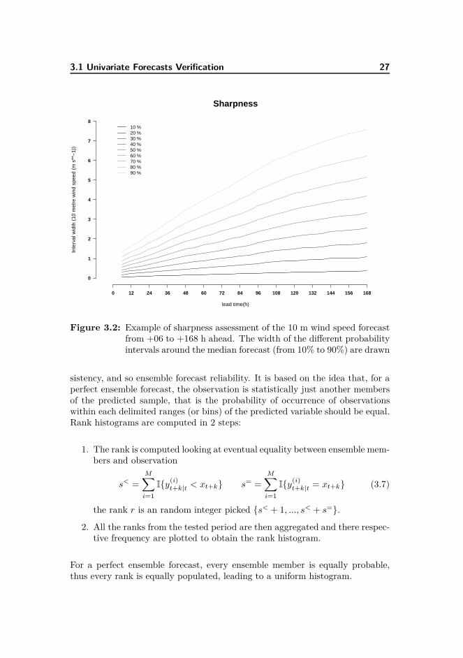
Sharpness Sharpness is a property of the forecast only, it does not dependson the observation. It characterises the ability of the forecast to deviate fromthe climatological probabilities. It is important for the ensemble spread not tobe wider than the climatological spread and not too sharp if it leads to a loss ofreliability. For an equal level of reliability, the sharper the better. Here, a wayto assess sharpness is to determine the width of two equidistant quantiles fromthe median.
Rank Histograms The Rank Histogram (also known as Talagrand Diagram)is not a score but a tool employed to qualitatively assess ensemble spread con-
3.1 Univariate Forecasts Verification 27
0 12 24 36 48 60 72 84 96 108 120 132 144 156 168
0
1
2
3
4
5
6
7
8
Sharpness
lead time(h)
Inte
rval
wid
th (
10 m
etre
win
d sp
eed
(m s
**−
1))
10 %20 %30 %40 %50 %60 %70 %80 %90 %
Figure 3.2: Example of sharpness assessment of the 10 m wind speed forecastfrom +06 to +168 h ahead. The width of the different probabilityintervals around the median forecast (from 10% to 90%) are drawn
sistency, and so ensemble forecast reliability. It is based on the idea that, for aperfect ensemble forecast, the observation is statistically just another membersof the predicted sample, that is the probability of occurrence of observationswithin each delimited ranges (or bins) of the predicted variable should be equal.Rank histograms are computed in 2 steps:
1. The rank is computed looking at eventual equality between ensemble mem-bers and observation
s< =
M∑
i=1
I{y(i)t+k|t < xt+k} s= =
M∑
i=1
I{y(i)t+k|t = xt+k} (3.7)
the rank r is an random integer picked {s< + 1, ..., s< + s=}.
2. All the ranks from the tested period are then aggregated and there respec-tive frequency are plotted to obtain the rank histogram.
For a perfect ensemble forecast, every ensemble member is equally probable,thus every rank is equally populated, leading to a uniform histogram.

28 Ensemble Forecast verification
Figure 3.3 shows an example of a rank histogram. The horizontal axis rep-0.
000
0.01
00.
020
0.03
0F
requ
ency
Figure 3.3: Example of a rank histogram with 95% consistency bars
resents the sorted bins of the M-members ensemble forecast system, and thevertical axis represents the probability of occurrence of observation into eachbin. The 95% consistency bars have been added to the figure. Consistency barsgive the potential range of empirical proportions that could be observed evenif dealing with perfectly reliable probabilistic forecasts. These intervals dependon the length of the period tested and are estimated as follows,
Ic =1
M+ 1.96
s√n
(3.8)
=1
M+ 1.96
√p(1 − p)
n(3.9)
=1
M+ 1.96
√1
M (1 − 1M )
n
with p the perfect probability of occurrence, M the number of ensemble mem-bers and n the number of valid observations. A rank histogram is consideredstatistically uniform if the probability of occurrence of each bins lies into theconsistency bars. It exists particular shapes of rank histograms :- If the too extreme bins are overpopulated (U shape), then the forecasts areunderdispersive because most of the observations fall outside of the ensemblerange.

3.1 Univariate Forecasts Verification 29
- If the middle bins are overpopulated (bell shape), then the forecasts are overdis-persive, observations do not enough fall into the extreme bins because the pre-dicted distribution is too wide.- If the lower bins are overpopulated, then the forecasts have a positive bias.- If the higher bins are overpopulated, then the forecasts have a negative bias.The figure 3.4 illustrates the previous list.
Obs
erve
d F
requ
ency
0.00
00.
010
0.02
00.
030
Obs
erve
d F
requ
ency
0.00
00.
010
0.02
00.
030
Obs
erve
d F
requ
ency
0.00
00.
010
0.02
00.
030
Obs
erve
d F
requ
ency
0.00
00.
010
0.02
00.
030
Figure 3.4: Usual kinds of rank histogram : negatively biased (top left), posi-tively biased (top right),underdispersive (bottom left), overdisper-sive (bottom right)
Reliability Index It exists a way to quantitatively assess reliablity. Thereliability index ∆, introduced by Delle Monache in 2006 (Delle Monache et al.,2006) quantifies the deviation of the rank histogram from uniformity.
∆k =
M∑
j=1
∣∣∣∣ξkj− 1
M + 1
∣∣∣∣ (3.10)
where ξkjis the observed relative frequency of the rank j for lead time k and M
the number of ensemble members. The Reliability index is a negatively orientedscore, with zero being the minimum value.

30 Ensemble Forecast verification
PIT Diagram The PIT diagram is equivalent to the rank histogram. It isthe most transparent way to illustrate the performance and characteristics ofa probabilistic forecast system. It represents the observed frequency of occur-rence conditional on predicted probabilities. The x-axis represents the predictedprobability and the y-axis the observed frequency. For instance, a point on thePIT diagram with coordinates (x = 0.9, y = 0.6) can be interpreted as the eventA predicted with a probability of 0.9 is actually observed only 6 times out of 10over the tested period. In that case, the forecast is not reliable. To be reliable,the event A predicted with probability 0.9 should be approximately observed 9times out of 10. For a perfect ensemble forecast system, predicted probabilityand observed probability should be identical, the PIT diagram should be rep-resented by the 45◦ straight line. As with the rank histogram, it exists severaltype of PIT diagrams: if the slope is to low, then the forecasts are underdisper-sive and if the slope is to high they are overdispersive.
0.0 0.1 0.2 0.3 0.4 0.5 0.6 0.7 0.8 0.9 1.00.0
0.1
0.2
0.3
0.4
0.5
0.6
0.7
0.8
0.9
1.0
+48h
nominal
empi
rical
observedideal
Figure 3.5: Example of a PIT diagram with the 95% consistency bars, thehorizontal axis represents the predicted probability the verticalaxis represents the observed probability
As well as for the rank histogram, consistency bars can be obtained thanks to theequation (3.10). However, contrary to the rank histogram all the consistencybars do not have the same width. Indeed, the perfect probability p is not

3.2 Multivariate Forecasts Verification 31
constant (from 0 to 1) and the product p(1 − p) evolves as a quadratic functionwith a maximum at p = 0.5. Consistency bars are therefore larger for thepredicted probability p = 0.5.
3.2 Multivariate Forecasts Verification
Multivariate forecasting needs specific multivariate verification. It exists sev-eral generalisations of univariate scores/tools permitting to assess the quality ofmultivariate forecasts.
Bivariate Root Mean Square Error The bivariate Root Mean Square Er-ror is the multivariate generalisation of the RMSE and is computed as follows:
bRMSE(k) =
√√√√ 1
N
N∑
t=1
‖yt+k|t − xt+k‖2 (3.11)
with yt|t−k and xt denoting the multivariate ensemble forecast mean vector andthe multivariate observation vector.
Bivariate Mean Absolute Error The bivariate Mean Absolute Error is themultivariate generalisation of the MAE and is computed as follows :
bMAE(k) =1
N
N∑
t=1
‖yt+k|t − xt+k‖ (3.12)
with yt+k|t and xt+k the multivariate ensemble forecast median vector and themultivariate observation vector.
Energy Score (es) The Energy Score is the multivariate generalisation ofthe Continuous Rank Probabilistic Score. It was introduced by Geniting andRaftery in 2007 (Gneiting and Raftery, 2007) and can be computed as follows :
es(f,x) = Ef ‖X − x‖β − 1
2Ef ‖X − X ′‖β (3.13)
Where X and X ′ are independent random vectors coming from the distributionf, x is the observation vector and β represents the dimension of the problem(3.13 reduces to the CRPS formulation when β = 1). The Energy score isa negatively oriented score, with zero being the minimum value. For a given

32 Ensemble Forecast verification
time and a give lead time, the energy score of a bivariate ensemble forecast,with (y(1)t+k|t,y
(2)t+k|t, . . . ,y(M)t+k|t) denoting the ensemble members, can
be written
es(ft+k|t,xt+k) =1
M
M∑
j=1
‖y(j)t+k|t−xt+k‖− 1
2M2
M∑
i=1
M∑
j=1
‖y(j)t+k|t−y
(i)t+k|t‖ (3.14)
However, while sampling a large number of outcomes from a predicted calibrateddistribution the computation of this score can be costly. In order to reduce thecomputation effort, a Monte Carlo approximation can be used. Then the energyscore can take the following form :
es(ft+k|t,xt+k) =1
K
K∑
j=1
‖y(j)t+k|t − xt+k‖ − 1
2(K − 1)
K−1∑
i=1
‖y(i)t+k|t − y
(i+1)t+k|t‖
(3.15)
where y(1)t+k|t, . . . , y
(K)t+k|t is a random sample of size K=10000 picked out from the
predicted probability density function ft+k|t .
Multivariate Rank Histogram A multivariate rank histogram (Gneitinget al., 2008) is the multivariate generalization of rank histogram seen above.It shares the same ideas : multivariate rank histogram of a calibrated forecastshould be uniform, multivariate rank histogram of underdispersive multivariateforecasts have an U shape and so on. Lets consider a multivariate ensembleforecast with the ensemble members yi and the observations x defined by vectors
that take values in Rd : yi = (y
(i)1 , y
(i)2 , . . . , y
(i)n ) and x = (x1, x2, . . . , xn).
x � y(i) if and only if xj � y(i)j for j = 1, 2, . . . , d.
Let suppose a bivariate ensemble forecasts as illustrated in figure 3.6, thenx � y(i) if and only if x belongs to the square to the left and below y(i). Thecomputation of the multivariate rank is a two step algorithm:
1. Assign pre-rank :We determine pre-rank ρj for each ensemble member:
ρj =
m∑
k=0
I{xk ≤ xj} (3.16)
where I{xk < xj} denotes the indicator function I with the conditionxk < xj . It is equal to 1 if the condition is true, 0 otherwise. Eachpre-rank is an integer between 1 and m+ 1.

3.2 Multivariate Forecasts Verification 33
Figure 3.6: Illustration of the computation of a bivariate rank histogram for aparticular ensemble forecast. (a) Ensemble forecast members andobservations with associated pre-ranks. The observations pre-rankis 3 because 3 of the 9 points belong to its lower left (observationsincluded). (b) From (a), four point have pre-rank ≤ 2, and twopoints have pre-rank 3, that is s< = 4 and s= = 2. Hence, the mul-tivariate rank is a random outcome of the set {5, 6} (source (Gneit-ing et al., 2008))
2. Find the multivariate rank :For the multivariate rank r, we note the rank of the observations, whilepossible ties are resolved at random:
s< =
m∑
j=0
I{ρj < ρ0} and s= =
m∑
j=0
I{ρj = ρ0} (3.17)
The multivariate rank r is chosen from a discrete uniform distribution onthe set {s< + 1, . . . , s< + s=} and is an integer between 1 and m+ 1.
3. Aggregate rank and plot multivariate rank histogram :We finally aggregate all multivariate ranks to plot the multivariate rankhistogram and add the 95% consistency bars.
The figure 3.7 show an positively biased multivariate ensemble forecasting sys-tem of wind speed and significant wave height for 48 h ahead at FINO1. There-fore, such a multivariate rank histogram suggests that the grey square at thebottom-left of figure 3.6 is rarely populated by ensemble vectors.

34 Ensemble Forecast verification0.
000.
040.
080.
12F
requ
ency
Figure 3.7: Example of Multivariate Rank Histogram for Wind speed +48 hforecast over FINO1
Multivariate Reliability Index As it is the case for univariate rank his-togram, a reliability index can be computed from equation (3.10) for any mul-tivariate rank histogram in order to quantitatively assess forecasts calibration.We call this index the multivariate reliability index.
Determinant Sharpness The determinant sharpness is the multivariate gen-eralization of the sharpness described previously. We use the same definition asemployed in (Möller et al., 2012), that is,
DS = (detΣ)1/(2d) (3.18)
where Σ is the empirical covariance matrix of a multivariate ensemble forecastfor a d-dimensional quantity.

3.3 Skill Score 35
3.3 Skill Score
The skill score is a way to directly compare one type of score for two differentmethods. For a given lead time k and a given score, the skill score is defined as:
SkillScore(k) = 1 − Score(k)
Score0(k)(3.19)
with Score(k) the score of the tested method and Score0(k) is the score ofthe benchmark method. Contrary to the other score presented before, the skillscore is always positively oriented, the higher the skill score, the better thetested method is compared to the benchmark. The maximum value of a skillscore is 1, it would indicate a perfect score for the tested method. A skill scoreof 0 would indicate that the tested method and the benchmark have the samescore, and a negative skill score would indicate that the tested method is worsethan the benchmark.

36 Ensemble Forecast verification

Chapter 4
Ensemble Forecast Calibration
Method
In this thesis, the main assumption is that Nature is not deterministic butprobabilistic. We assume that at a time t+k, Nature chooses a distributionGt+k, representing the uncertainty of the atmospheric conditions, and picks outone random number from that distribution to obtain the observation xt+k. We
also assume that the ensemble forecast members y(j)t+k|t are outcomes from a
predicted distribution Ft+k|t that tries to estimate Gt+k. The goal of ensembleforecasting is to predict the closest distribution Ft+k|t to the one chosen bythe Nature Gt+k. However, ensemble forecasts tend to be uncalibrated (i.e.biased and underdispersive), which means that the mean and the spread of thepredicted probability distribution show systematic errors. Therefore, we proposesome calibration methods that aim at reducing those errors.
The first assumption of our model is that given a variable (wind speed or waveheight), the distributions {Gt1
, Gt2, . . . , Gtn
} chosen by the Nature to obtainthe observation for the times {t1, t2, . . . , tn} are of the same type and only differfrom their parameters. The goal of our calibration method is to fit a distribu-tion conditional on the ensemble mean and the ensemble variance. Therefore,we do a first approximation by fitting a distribution to sets of observed windspeed and significant wave height, conditional on the predicted ensemble meanbeing within some bins. In order to assess the representativeness of the chosendistribution for the different variables, we use quantile-quantile plots.

38 Ensemble Forecast Calibration Method
Quantile-Quantile plots (Q-Q plot) (Wilks, 2006) compare quantiles (inversefunction of the cumulative density function) of an empirical data with quan-tiles of a distribution function with parameters being representative of the data.It is an indirect way of comparing two density functions. The horizontal axisrepresents the quantiles (dimension values) of the mathematical distributionfunction, and the vertical axis represents the quantiles estimated from the em-pirical data. A Q-Q plot of two samples coming from the same distributionwould show points around the diagonal confirming that the quantiles of the twosamples are similar.
0 2 4 6 8
0
2
4
6
8
Truncated Normal Quantiles
Obs
erve
d Q
uant
iles
observationsforecasts
Ensemble mean Q 1
2 4 6 8 10
2
4
6
8
10
Truncated Normal Quantiles
Obs
erve
d Q
uant
iles
observationsforecasts
Ensemble mean Q 2
4 6 8 10 12 14
468
101214
Truncated Normal Quantiles
Obs
erve
d Q
uant
iles
observationsforecasts
Ensemble mean Q 3
6 8 10 12 14 16 18
68
1012141618
Truncated Normal Quantiles
Obs
erve
d Q
uant
iles
observationsforecasts
Ensemble mean Q 4
Figure 4.1: Q-Q plots for observed and predicted 10 m wind speeds conditionalon the 10 m wind speed ensemble mean being in the four quartilesdenoted Q1,Q2,Q3 and Q4 compared with a truncated normaldistribution. Data used covers the period from January 2010 toDecember 2010.

39
0.2 0.4 0.6 0.8 1.0 1.2
0.20.40.60.81.01.2
Truncated Normal Quantiles
Obs
erve
d Q
uant
iles
observationsforecasts
Ensemble mean Q 1
0.4 0.6 0.8 1.0 1.2 1.4 1.6
0.40.60.81.01.21.41.6
Truncated Normal Quantiles
Obs
erve
d Q
uant
iles
observationsforecasts
Ensemble mean Q 2
1.0 1.5 2.0 2.5
1.0
1.5
2.0
2.5
Truncated Normal Quantiles
Obs
erve
d Q
uant
iles
observationsforecasts
Ensemble mean Q 3
1.0 1.5 2.0 2.5 3.0 3.5 4.0
1.01.52.02.53.03.54.0
Truncated Normal Quantiles
Obs
erve
d Q
uant
iles
observationsforecasts
Ensemble mean Q 4
Figure 4.2: Q-Q plots for observed and predicted significant wave height con-ditional on the significant wave height ensemble mean being inthe four quartiles denoted Q1,Q2,Q3 and Q4 compared with atruncated normal distribution. Data used covers the period fromJanuary 2010 to December 2010.
Figures 4.1 and 4.2 show the Q-Q plots comparing 10 m wind speed and sig-nificant wave height 48 hours ahead forecasts and observations of the year 2010with the a truncated normal distribution with a lower bound at zero, fitted bythe maximum likelihood technique (see Chapter 4.1). The data has been splitinto 4 bins corresponding to the four quartiles (25%,50%,75% and 100%) of theensemble forecast mean. In the figures quantiles lies around the diagonal con-firming that both variables sample the distributions tested. Thus, we chooseto model significant wave height and 10 m wind speed as sampling truncatednormal distributions with a cut off at zero for both variables. It can noticed onfigure 4.1 that the 10 m wind speed ensemble members does not predict speedsbelow 2m.s−1, which is certainly due to the ECMWF parametrisation of thisvariable. However, there is no valuable reason for the wind not to blow be-low that speed at that height, plus our wind speed extrapolation might providewind speeds between 0 and 2 m.s−1. The truncation for the 10 m wind speedis therefore chosen at 0 m.s−1 and not at 2 m.s−1.

40 Ensemble Forecast Calibration Method
4.1 Univariate Calibration CAL1
After analysis of the QQ-plots for every lead times, we assume then that each
observations xt+k, as well as each ensemble member y(j)t+k|t, sample a truncated
normal distribution with a cut-off at zero as employed in (Thorarinsdottir andGneiting, 2008). Thus, the non-negativity of wind speed and significant waveheight is respected.
xt+k ∼ N0(µt+k, σ2t+k) yt+k|t ∼ N0(µt+k|t, σ
2t+k|t) (4.1)
The truncated normal distribution is the probability distribution of a normallydistributed variable whose value is either bounded below or above (or both).Here, only a lower boundary at zero is used. The distribution is defined by twoparameters. The parameters µ and σ2 are respectively the location parameterand the scale parameter. They represent the mean and the variance of the un-derlying normal distribution (non truncated) and are slightly different from thetruncated mean and the truncated variance. The probability density functionof the truncated normal distribution is given by
f0(y) =1
σ
ϕ(
y−µσ
)
Φ(
µσ
) for y > 0 (4.2)
f0(y) = 0 otherwise. Here, ϕ and Φ respectively denote the standard probabilityand cumulative density functions of the normal distribution.The first two moments of the truncated normal distribution with a cut-off at
zero can be computed as follows,
µ0 = µ+ϕ(µ
σ )
Φ(µσ )σ (4.3)
σ20 = σ2 − σ2 ϕ(µ
σ )
Φ(µσ )
[1 +
µ
σ
](4.4)
The closer the sample of the distribution to zero, the more the two first momentsof the truncated normal distribution µ0 and σ2
0 differ from the moments of theunderlying normal distribution µ and σ2.
Given a lead time k, we assume that the location parameter of the observationµt+k is a linear function of the predicted mean yt+k|t. We choose not to followexactly the idea of Thorarinsdottir (Thorarinsdottir and Gneiting, 2008) whobuilds a multiple linear model taking every ensemble members as predictors forthe location parameter estimation. Considering the large number of ensemblemembers of the EPS (51 members) compared to the ensemble forecasting sys-tem used by Thorarinsdottir (8 members of the UWME), we choose to restrict

4.1 Univariate Calibration CAL1 41
x
prob
abili
ty d
ensi
ty
0 5 10 15
0.0
0.1
0.2
0.3
0.4
0.5 µ=1, σ=1
µ=2, σ=2µ=5, σ=4
Figure 4.3: Examples of univariate truncated normal distributions with dif-ferent location and spread parameters.
the predictors only to the ensemble mean. Therefore the model for the meancorrection can be written as follows :
µt+k = a+ byt+k|t (4.5)
The mean correcting parameters a and b reflect the relationship between theensemble mean and the location parameter during the training period. It has tobe noted that even if wind speed and significant wave height are non negativevariables, the location parameter of the truncated normal distribution does nothave to be positive. Indeed, µ ∈ R and the parameters a and b are then uncon-strained.
Furthermore, the spread parameter of the observation σ2t+k is also assumed to
be a linear function of the predicted variance s2t+k|t.
σ2t+k = c+ ds2
t+k|t (4.6)
The parameters c and d reflect the relationship between the ensemble spreadand the forecast error during the training period. When the correlation is im-portant between those two, d is high and c is small, when the ensemble variance

42 Ensemble Forecast Calibration Method
information is not useful, d tends to be smaller and c to be higher. c and d
are constrained to be non negative because of the positive nature of the secondorder moment. The non-negativity of the parameters c and d is guaranteed bywriting c = γ2 and d = δ2.Thus the calibrated forecast y∗
t+k|t should take the form of a truncated normaldistribution with the corrected parameters,
y∗t+k|t ∼ N0(a+ byt+k|t, c+ ds2
t+k|t) (4.7)
This model is not rigorously correct in the sense that the linear models shouldinvolve the true truncated mean and the true truncated variance instead of thelocation and spread parameters. However, The wind speed and the significantwave height rarely reach the lower boundary (zero), and so the location param-eter µ and the truncated mean µ0 do not significantly differs. It is also true forthe spread parameter σ2 and the truncated variance σ2
0 .
The estimation of those four correcting parameters can be done in differentways. (Gneiting et al., 2005; Thorarinsdottir and Gneiting, 2008) employed aminimum CRPS estimation, that is the parameters are estimated in such a waythat they minimise the CRPS score over the estimation period. However, such atechnique can not be employed for bivariate distributions. So, out of concern ofconsistency between the univariate and bivariate calibration methods, we chooseto use maximum likelihood estimation. The maximum likelihood estimation isa popular method used to estimate the parameters of a mathematical function(often a distribution function). The parameters issued from the maximum like-lihood estimation are supposed to be the most probable parameters given theobserved data.Let suppose that (x1, ..., xn) xi ∈ R
d is an independent and identically dis-tributed sample coming from a statistical distribution with a probability den-sity function {pθ : θ ∈ Θ} in R
d. θ is the parameter (scalar or vector) to beestimated. For a single observation xi, the likelihood function is identical to theprobability density function. The only difference is that the pdf is a functionof the data (parameters being fixed) whereas the likelihood function is a func-tion of the unknown parameters (data being fixed). The likelihood function ofa distribution given a sample of n independent values is the product of the nindividual likelihood functions :
L(θ|x1, ..., xn) = p(x1|θ) × p(x2|θ) × ...× p(xn|θ)
=
n∏
i=1
p(xi|θ) (4.8)
We use a slightly different method which is a combination of maximum likeli-hood estimation techniques (Pawitan, 2001). Instead of having a sample of nobservations from one and only statistical distribution with a probability density

4.1 Univariate Calibration CAL1 43
function pθ, we have n independent observations (x1, ..., xn) sampling n differentstatistical distributions which share the same parameter θ with the respectiveprobability density functions (pi,θ, ..., pn,θ). Then the likelihood function be-comes :
L(θ|x1, ..., xn) =
n∏
i=1
pi(xi|θ) (4.9)
where pi(xi|θ) represents the individual likelihood function of the pair (xi,θ),equal to the probability density function of the distribution that xi is samplingwith the parameter θ.
Generally, we work with the log-likelihood function which is the sum of thelogarithm of the individual likelihood functions :
ln(L(θ|x1, ..., xn)) = ln(
n∏
i=1
pi(xi|θ))
=
n∑
i=1
ln(pi(xi|θ)) (4.10)
In these functions (likelihood and log-likelihood), the observed values x1, ..., xn
are the fixed parameters and θ is actually the variable. The maximum likelihoodestimation finds the best estimator of θ by maximising the likelihood (or log-likelihood) function:
θmle = argmaxθ∈Θ
L(θ|x1, ..., xn) (4.11)
θmle is the statistically most probable estimator of θ.
In our case, that is the correction of the ensemble mean and variance, pi(xi|θ)is equal to the probability density function of a truncated normal distributionN 0(a + byt+k|t, c + dst+k|t) seen in equation (4.2). Then, the log-likelihoodfunction that has to be maximised can be written as follows:
L(a, b, γ, δ) =n∑
i=1
ln
(1
σ
ϕ(y−µσ )
Φ(µσ )
)
=
n∑
i=1
(− ln σ + lnϕ(
y − µ
σ) − ln Φ(
µ
σ)
)
=
n∑
i=1
(− 1
2ln(γ2 + δ2s2
i )
+ lnϕ( y − a+ byi√
γ2 + δ2s2i
)− ln Φ
( a+ byi√γ2 + δ2s2
i
))
(4.12)

44 Ensemble Forecast Calibration Method
c = γ2 and d = δ2
with n being the length of the training period, a, b, γ and δ some unconstrainedparameters. Of course, this method can only be employed if we assume thatforecasts errors are independent in time. However, as explained in (Rafteryet al., 2005), estimates are unlikely to be sensitive to this assumption becausecalibration is done for one particular time only and not several simultaneously.The optimization algorithm used to estimate the four parameters for every fore-cast needs starting values and the solution might be sensitive to those initialvalues.Therefore, we use the parameters from the previous estimation day asstarting values. This allows a faster convergence of the algorithm and a betterconsistency in the evolution of the parameters from one day to the other. Inthis report, this univariate calibration method is called CAL1.
4.2 Bivariate Calibration 45
4.2 Bivariate Calibration
We have seen in chapter 2 that surface wind speed and significant wave heightare, in a certain way, correlated. Wind-waves are created by the local winds andare then strongly correlated to surface wind speed, but swell was created in an-other location and a few hours or days before by different winds and thus mightbe uncorrelated to local wind speed. Since it calibrates one variable at a time,the univariate calibration method does not take into account the correlationand therefore predicts uncorrelated bivariate forecasts. The idea of a bivariatecalibration is to jointly calibrate the variables so their existing correlation is notviolated.
Bivariate calibration of weather forecasts is a new field of researches that onlya few scientists have investigated to this day. Pinson (Pinson, 2012) used abivariate EMOS to calibrate the u and v components of wind. Assuming thatthe joint distribution of the two components of the wind is a bivariate normaldistribution, he did not modify the predicted correlation but corrected the meanof each component through a linear function with the two predicted means aspredictor. Möller (Möller et al., 2012) used Gaussian copula to introduce abivariate calibration after having marginally calibrated different variables liketemperature, wind speed and precipitation. She showed that the dependencelost during marginal calibration of any weather variable can be recovered usinggaussian copula. The correlation of the copula is estimated from the trainingperiod. Schuhen (Schuhen et al., 2012) also jointly calibrated the u and v com-ponent. Like Pinson, she assumed that wind vectors sample a bivariate normaldistribution. However, instead of using a predicted correlation she showed thatcorrelation could be estimated through a sinusoidal function of the ensemblemean wind direction.
In this thesis, we create a bivariate calibration method that aims at calibrating10 m wind speed and significant wave height while taking into account theirpredicted correlation. We assume that vectors defined by 10 m wind speedand significant wave height sample a truncated bivariate normal distributionwith a lower bound at zero for both components (Horrace, 2005; Wilhelm andManjunath, 2010). We denote Y the two components forecast vector samplinga truncated bivariate normal distribution.
Y ∼ N 02 (µt+k|t, Σt+k|t) (4.13)
with µt+k|t the two components predicted mean vector with the first compo-
nent for the wind (µu) and the second for the wave height (µh). Σt+k|t is the

46 Ensemble Forecast Calibration Method
predicted variance-covariance matrix with the variances on the diagonal and thecovariances outside of the diagonal.
µt+k|t =
(µu,t+k|t
µh,t+k|t
)(4.14)
Σt+k|t =
(σ2
u,t+k|t ρt+k|tσu,t+k|tσh,t+k|t
ρt+k|tσu,t+k|tσh,t+k|t σ2h,t+k|t
)(4.15)
Indices u and h respectively denote the 10 m wind speed and the significantwave height component.Given boundaries, the truncated bivariate normal distribution is then fully de-scribed by 5 parameters:
1. the mean value for the two components µu and µh
2. the variance for two components σ2u and σ2
h
3. the correlation between the two components ρ
The probability density function of the truncated bivariate normal distributioncan be written as follows:
f0(y) =exp{−1
2(y − µ)Σ−1(y − µ)}
∫∫∞
0exp{−1
2(y − µ)Σ−1(y − µ)}dx
(4.16)
Two examples of truncated bivariate normal distribution with a cut-off at zerofor both dimensions are illustrated in figure 4.4.
The models for the correction of the predicted mean and the predicted varianceremain identical to the univariate calibration:
µu,t+k = au + buyu,t+k|t (4.17)
µh,t+k = ah + bhyh,t+k|t (4.18)
σ2u,t+k = cu + dus
2u,t+k|t (4.19)
σ2h,t+k = ch + dhs
2h,t+k|t (4.20)
The parameters cu,du,ch and dh have to be non-negative in order to ensure thatthe mean and the variance are positive. Thus we write cu = γ2
u,du = δ2u,ch = γ2
h

4.2 Bivariate Calibration 47
x1
x 2
0.02
0.04
0.06
0.08
0 2 4 6 8 10
02
46
810
12
0.01
0.02
0.03
0.04
0.05
µ1=5, µ2=2, σ12=2, σ2
2=3, σ12=1µ1=5, µ2=6, σ1
2=4, σ22=5, σ12=2
Figure 4.4: Example of a truncated bivariate normal distribution with a cut-off at zero for both dimensions.
and dh = δ2h which leads to
µu,t+k = au + buyu,t+k|t (4.21)
µh,t+k = ah + bhyh,t+k|t (4.22)
σ2u,t+k = γ2
u + δ2us
2u,t+k|t (4.23)
σ2h,t+k = γ2
h + δ2hs
2h,t+k|t (4.24)
The last parameter to deal with is the correlation ρ. We propose here twodifferent ways of taking the correlation into account. Firstly, we propose toestimate the correcting parameters while forcing the correlation to be equal tothe predicted one, maximum likelihood technique is employed using the trun-cated bivariate distribution. A second approach is envisaged, we propose tomarginally estimate the correcting parameter as for the univariate calibrationmethod CAL1 and then recover the lost dependence using the bivariate trun-cated distribution with the raw predicted correlation.

48 Ensemble Forecast Calibration Method
4.2.1 Joint Calibration method CAL2
We choose to build a bivariate calibration method that take into account thepredicted correlation without correcting it. The true correlation is assumed tobe identical to the predicted one. So we write :
ρt+k = ρt+k|t (4.25)
Thus the calibration method does not violate the existing relationship betweenwind speed and wave height. Of course, as it has been discussed for the uni-variate calibration method, it is not strictly correct since the correlation of theunderlying normal distribution and the correlation of the truncated normal dis-tribution are not exactly identical. Indeed, the closer to the boundaries theensemble members are, the more different the two correlation are. However,this assumption is relevant in the sense that ensemble members of wind speedand significant wave height are rarely close to the lower boundary (zero). Thecorrelation being hold fixed, the calibration method has to estimated 8 pa-rameters (4 for the mean vector correction and 4 for the variance-covariancematrix). As it has been done for the univariate calibration method, parametersau,bu,cu,du,ah,bh,ch,dh are estimated through maximum likelihood techniquewith the correlation as a fixed parameter. The function to maximise can bewritten as follows,
L(η) =
n∑
i=1
[ln(f(η|xi,µi,Σi)
)]
where f denotes the density of the truncated bivariate normal predicted distribu-tion, η = (au, bu, γu, δu, ah, bh, γh, δh)T the parameter vector, x the observationvector, µ the predicted mean vector, Σ the predicted variance-covariance ma-trix for all forecasts contained in the training period of n events.
L(η) =n∑
i=1
[ln( exp{−1
2(xi − µi)Σ
−1i (xi − µi)}
∫∫∞
0 exp{−1
2(yi − µi)Σ
−1i (yi − µi)}dx
)](4.26)
=
n∑
i=1
[− ln
(∫∫ ∞
0
exp{−1
2(xi − µi)Σ
−1i (xi − µi)}dx
)
−1
2(xi − µi)Σ
−1i (xi − µi)
]

4.2 Bivariate Calibration 49
with
− 1
2(xi − µi)Σ
−1i (xi − µi) =
(xu,i − µu,i
xh,i − µh,i
)T (σ2
u,i ρiσu,iσh,i
ρiσu,iσh,i σ2h,i
)−1(xu,i − µu,i
xh,i − µh,i
)
= − (xu,i − au + buyu,i)2
2(1 − ρ2i )(γ2
u + δ2us
2u,i)
− (xh,i − ah + bhyh,i)2
2(1 − ρ2i )(γ2
h + δ2hs
2h,i)
+ρi(xu,i − au + buyu,i)(xh,i − ah + bhyh,i)
(1 − ρ2i )√
(γ2u + δ2
us2u,i)(γ
2h + δ2
hs2h,i)
The correlation parameter ρ of the truncated bivariate normal distribution isfixed. The maximum likelihood estimation finds the values for the parametersunder which the probability that the training data would have been observedis maximal. Since the number of parameter is higher, the estimation is muchmore sensitive and the computation time more costly than for the univariatemethod, it is even more important to find appropriate initial values to start theoptimization. Therefore, it is even more important that parameters from theprevious estimation are used as input to initiate the algorithm. In this report,this bivariate calibration method is called CAL2.
4.2.2 EPS-prescribed correlation approach CAL1+
In a second approach, we choose to combine marginally calibrated forecasts anduse the predicted correlation to recover the dependence during the univariate cal-ibration method. The method is similar to the one proposed by Möller (Mölleret al., 2012). In order to obtain a joint predictive distribution of 10 m windspeed and significant wave height, each variable is individually calibrated asdescribed in Chapter 4.1 without considering nor the other variable neither thecorrelation existing between the two of them. Then in a second step, the de-pendence lost during the estimation of the correcting parameters is recoveredby sampling a truncated bivariate normal distribution (equation(4.16)) with themarginally estimated parameters and the correlation prescribed by the raw fore-casts. Therefore, this calibration method will share the same univariate scoresthan the univariate calibration method but intend to improve the bivariate pat-tern of the forecasts. Contrary to Möller who used a correlation estimated fromthe training period, we use the correlation predicted by the EPS for the validdate which allow a more dynamic correction. In this report, this method iscalled CAL1+.

50 Ensemble Forecast Calibration Method

Chapter 5
Results
In this chapter, the results of the different calibration methods applied on theEPS forecasts the ECMWF for the specific FINO1 location are exposed. Fore-casts have been tested over the 1855 forecasts events of the period 2010-2011when both 10 m wind speed and significant wave height were both available.Calibration methods are systematically compared with the raw ensemble fore-casts and the climatology benchmark. The verification tools/scores describedin Chapter 3 are used to assess the different forecast types. We first assess theunivariate calibration method for lead times from 6 to 168 hours ahead withunivariate scores/tools and then expose the results of the bivariate calibrationmethods for the 48 hours ahead prediction horizon.
5.1 Benchmarking
A benchmark is defined by a very simple model that can used in forecasting.The climatology forecast is a type of probabilistic forecasts that is often used asa benchmark because of it simplicity. It consists in forecasting, the pdf of theclimatology, that is a non parametric density function estimated from the pastobservations. The climatology forecast is by definition reliable, but not sharp.It is not flow dependent and therefore the predicted pdf is always identical.

52 Results
Figure 5.1: Three dimensional representation of the climatology benchmarkforecast. The vertical axis represents the number of occurence perbin. This histogram has been computed with the 1855 pairs ofwind speed - wave height observations available over the period2010-2011.
The Climatology forecasts is defined by the same parameters shown in table 5.1and the same distribution seen in figure 5.1 for every day and every predictionhorizon.
µu µh σ2u σ2
h ρ
7.33 1.39 12.73 0.70 0.72
Table 5.1: Parameters of the climatology benchmark computed over the entireperiod 2010-2011

5.2 Univariate Calibration Method 53
5.2 Univariate Calibration Method
10 m wind speed and significant wave height ensemble forecasts are marginallycalibrated with the calibration method CAL1 detailed in Chapter 3.1, that iscalibrated forecasts are obtained individually for every variable by fitting a trun-cated univariate distribution with corrected parameters. Correcting parametersare estimated from the training period and applied on every forecasts duringthe years 2010 and 2011.
The small amount of data suggests using a sliding window technique to esti-mate the correcting parameters in which the training data consists in the recentpast. The optimal length of the training period depends on the variability of theatmospheric conditions on the site of interest. A short training period wouldsuggest a fast adaptivity to seasonal variation whereas a long training periodwould reduce the variability of the parameter estimation. There does not existan automatic way to find the optimal length for the training period. Thus, in or-der to estimate the most appropriate length, different lengths of training periodfrom 20 days to 60 days have been tested, as proposed in (Schuhen et al., 2012)and the mean energy score (average on every lead times) has been computed forevery simulation.As suggested by the figure 5.2, the optimal length of the training period min-
imising the energy score of the marginally calibrated forecasts is approximatively42 days. Thus the correcting parameters for day d are estimated on the periodbetween day d− 1 and d− 43. However, the length of the training period beingalways equal to 42 days, if the data on day d− 10, for instance, is not available,then the training data set covers the period from day d− 1 to day d− 44. Con-sidering the fact that two ensemble forecasts are issued per days at ECMWF(one at 00UT C and the other at 12UT C), a 42 days training period consists in84 forecast events.
Figure 5.3 illustrate the marginal calibration of an ensemble forecast of surfacewind speed issued on the 14th of July 2010 at 00UT C for the 16th of July 2010at 00UT C(48 hours ahead). The two forecasts are assumed to sample truncatednormal distributions. The coefficients au, bu, cu, and du for the correspondingday can be seen in table 5.2. They have been estimated from the training periodincluding 84 forecasts from the 2nd of June and the 14th of July 2010 and havebeen applied to the raw forecast (blue) in order to obtain the calibrated one(red). The ensemble mean has been translated from 8.2 m.s−1 to 7.5 m.s−1
whereas the corresponding wind speed observation is 7.2 m.s−1. As it is indi-cated by the highest density of the calibrated distribution, the ensemble spreadhas been dilated.

54 Results
20 30 40 50 60
1.39
01.
395
1.40
01.
405
1.41
01.
415
days
Ene
rgy
scor
e
Figure 5.2: Mean Energy score (average on every lead times) of the marginallycalibrated 10 m wind speed and significant wave height forecastsas a function of the length of the training period.
au bu cu du
0.24 0.87 0.76 0.84
Table 5.2: Parameters estimates of the univariate calibration CAL1 of a 48hours ahead wind speed EPS forecast valid on the 16th of July2010 at 00UT C .
The first goal of any calibration method is to obtain reliable ensemble forecasts,i.e equally likely to occur ensemble members. As explained in Chapter 3, re-liability can be qualitatively assessed by rank histograms and PIT diagrams.Figures 5.4 and 5.5 show a comparison of the univariate rank histograms andPIT diagrams of the different 48 hours ahead 10 m wind speed and significantwave height forecasts aggregated over the year 2010 and 2011.

5.2 Univariate Calibration Method 55
0 5 10 15
RawCalibratedObservations
10 metre wind speed
Figure 5.3: Example of univariate calibration of a 48 hours ahead ensem-ble forecast of 10m wind speed valid on the 16th of July 2010at 00UT C . The vertical bars represent the predicted means, thecurves represent the forecast pdfs, the blue elements correspond tothe EPS and the red ones to the CAL1 forecast. The correspond-ing observation is symbolised by the yellow point on the x-axis.

56 Results
While wind speed and wave height raw forecasts are both very underdipsersive,as indicated by the U shape of the respective rank histograms and the smallslope of the corresponding PIT diagrams, the other types of forecasts seem cali-brated. Indeed other rank histograms are relatively close to uniformity and PITdiagrams close to the diagonal. After calibration, ensemble forecasts provide re-liable univariate probabilistic information about the future weather conditions,which means that every ensemble member is equally likely to occur and the pre-dicted quantiles are statistically representative of the uncertainty. Apart fromthe first bin which is slightly overpopulated, i.e over the top of the consistencyinterval, every other rank lies into it. The climatology benchmark is perfectlycalibrated with every bin being into the consistency interval and a PIT diagramalmost indistinguishable from the diagonal. In these figures, we can not clearlycompare CAL1 reliability with the climatology reliability. However, reliabilityimprovements can be summarised and quantitatively assessed for every leadtime thanks to the reliability index.

5.2 Univariate Calibration Method 57
0.00
0.05
0.10
0.15
Fre
quen
cy
(a) EPS
0.0 0.1 0.2 0.3 0.4 0.5 0.6 0.7 0.8 0.9 1.00.0
0.1
0.2
0.3
0.4
0.5
0.6
0.7
0.8
0.9
1.0
+48h
nominalem
piric
al
observedideal
(b) EPS
0.00
0.01
0.02
0.03
Fre
quen
cy
(c) Climatology
0.0 0.1 0.2 0.3 0.4 0.5 0.6 0.7 0.8 0.9 1.00.0
0.1
0.2
0.3
0.4
0.5
0.6
0.7
0.8
0.9
1.0
+48h
nominal
empi
rical
observedideal
(d) Climatology
0.00
0.01
0.02
0.03
Fre
quen
cy
(e) CAL1
0.0 0.1 0.2 0.3 0.4 0.5 0.6 0.7 0.8 0.9 1.00.0
0.1
0.2
0.3
0.4
0.5
0.6
0.7
0.8
0.9
1.0
+48h
nominal
empi
rical
observedideal
(f) CAL1
Figure 5.4: Rank Histograms and PIT diagrams of the 48 hours ahead 10 mwind speed (a) raw forecasts, (b) climatology, and (c) marginallycalibrated forecasts

58 Results0.
000.
020.
040.
060.
08F
requ
ency
(a) EPS
0.0 0.1 0.2 0.3 0.4 0.5 0.6 0.7 0.8 0.9 1.00.0
0.1
0.2
0.3
0.4
0.5
0.6
0.7
0.8
0.9
1.0
+48h
nominal
empi
rical
observedideal
(b) EPS
0.00
0.01
0.02
0.03
Fre
quen
cy
(c) Climatology
0.0 0.1 0.2 0.3 0.4 0.5 0.6 0.7 0.8 0.9 1.00.0
0.1
0.2
0.3
0.4
0.5
0.6
0.7
0.8
0.9
1.0
+48h
nominal
empi
rical
observedideal
(d) Climatology
0.00
0.01
0.02
0.03
Fre
quen
cy
(e) CAL1
0.0 0.1 0.2 0.3 0.4 0.5 0.6 0.7 0.8 0.9 1.00.0
0.1
0.2
0.3
0.4
0.5
0.6
0.7
0.8
0.9
1.0
+48h
nominal
empi
rical
observedideal
(f) CAL1
Figure 5.5: Rank Histograms and PIT diagrams of 48 hours ahead significantwave height (a) raw forecasts, (b) climatology, and (b) marginallycalibrated forecasts

5.2 Univariate Calibration Method 59
0 50 100 1500.0
0.2
0.4
0.6
0.8
1.0
1.2
lead time
Rel
iabi
lity
Inde
x
(a) Reliability Index
0 50 100 150
−40
−20
0
20
40
60
80
lead time
Ski
ll R
elia
bilit
y In
dex
(%)
(b) Skill Reliability Index against raw forecasts
Figure 5.6: Quantitative reliability assessment of the different univariate fore-casts types. (a) Evolution of the reliability index with the predic-tive horizon of the EPS (black), climatology benchmark (green)and CAL1 forecast (red) for 10 m wind speed (triangle) and sig-nificant wave height (circle). (b) Skill reliability index of themarginally calibrated forecasts CAL1 against the raw forecasts for10 m wind speed (triangle) and significant wave height (circle).

60 Results
Figure 5.6(b) shows the evolution of the reliability index improvements with theprediction horizon for the same types of forecasts than in the previous figures.The climatology benchmark has the best reliability index (< 0.05 for every leadtime) of the three forecasts types. Forecast reliability is considerably improvedby the univariate calibration method CAL1 for both variables. Indeed, signif-icant improvements of more than 80% can be noticed for the firsts lead timesof both 10 m wind speed and significant wave height forecasts. These improve-ments remains more or less constant for medium range for 10 m wind speedwhereas they decrease much faster for the significant wave height. In can benoticed that raw ensembles forecasts tend toward the climatology for long pre-diction horizon and are therefore already more or less calibrated.After calibration, the forecasts are unbiased.Table 5.3 shows the bias score of the different forecast types for the 48 hours
Significant Wave HeightEPS 0.025
Climatology -0.023CAL1 0.019
10 m Wind SpeedRaw forecast 0.355Climatology -0.045
CAL1 -0.018
Table 5.3: Bias of the different forecast types for the 48 hours ahead horizon
ahead horizon. The bias is similar for every lead times and is therefore onlyexposed for one lead time (48 hours horizon). The marginally calibrated fore-casts CAL1 performs all types of forecasts. Even if significant wave height rawforecasts are much less biased (0.025 m) than the 10 m wind speed forecasts(0.355 m.s−1), calibration allows bias decrease for both variables. CAL1 evenperforms the climatology forecast. Indeed, the climatology benchmark has beencomputed over less than two years of data and is therefore less accurate.
While bias only informs about the systematic errors, RMSE assesses errorsamplitude giving more weight to large errors. Improvements of the RMSE as afunction of the prediction horizon are depicted in the figure 5.7 for the 10 m windspeed and the significant wave height. The skill RMSE of the marginally cali-brated forecasts CAL1 against raw forecasts has been computed over the entireperiod 2010-2011. Calibrated forecasts predict better ensemble means resultingresulting in improvements of the RMSE. The most significant improvementscan be seen for the first lead times where calibration allows a decrease of theRMSE of approximately 5% for both variables. These improvements are moresignificant for the wave forecasts. It can also be noticed an oscillation in theskill RMSE for both variables. Indeed, since the EPS is issued twice a day and
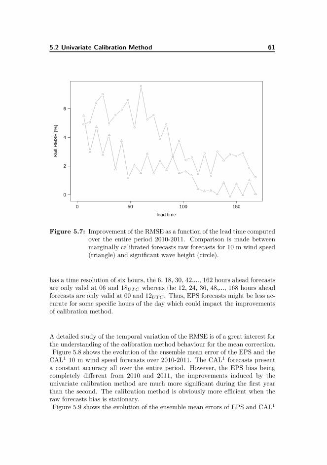
5.2 Univariate Calibration Method 61
0 50 100 150
0
2
4
6
lead time
Ski
ll R
MS
E (
%)
Figure 5.7: Improvement of the RMSE as a function of the lead time computedover the entire period 2010-2011. Comparison is made betweenmarginally calibrated forecasts raw forecasts for 10 m wind speed(triangle) and significant wave height (circle).
has a time resolution of six hours, the 6, 18, 30, 42,..., 162 hours ahead forecastsare only valid at 06 and 18UT C whereas the 12, 24, 36, 48,..., 168 hours aheadforecasts are only valid at 00 and 12UT C . Thus, EPS forecasts might be less ac-curate for some specific hours of the day which could impact the improvementsof calibration method.
A detailed study of the temporal variation of the RMSE is of a great interest forthe understanding of the calibration method behaviour for the mean correction.Figure 5.8 shows the evolution of the ensemble mean error of the EPS and the
CAL1 10 m wind speed forecasts over 2010-2011. The CAL1 forecasts presenta constant accuracy all over the entire period. However, the EPS bias beingcompletely different from 2010 and 2011, the improvements induced by theunivariate calibration method are much more significant during the first yearthan the second. The calibration method is obviously more efficient when theraw forecasts bias is stationary.Figure 5.9 shows the evolution of the ensemble mean errors of EPS and CAL1

62 Results
Ens
embl
e m
ean
erro
r
01/2010 01/2011 01/2012
−10
−8
−6
−4
−2
0
2
4
6
8
Figure 5.8: Comparison of 10 m wind speed ensemble mean errors over 2010-2011. The black line is the ensemble mean errors of the raw fore-casts, the red line is the smoothed ensemble mean errors of thesame forecast and the green line is the smoothed ensemble meanerrors after marginal calibration.
significant wave height forecasts. It can be seen that the calibration is moreefficient than for the wind speed 5.8. Indeed, the EPS bias from one month tothe other is much less fluctuating than for the wind speed and is therefore easierthe correct.
The CRPS is a score that is affected by both mean and variance correction.In other words, the CRPS is impacted by the entire predicted distribution andtherefore allows an overall univariate assessment of the marginal calibrationmethod CAL1. Figure 5.10 presents the improvements of the CRPS obtainedthrough marginal calibration for both 10 m wind speed forecasts and significantwave height. The calibration efficiency is much more significant for the CRPSthan for other scores. Indeed, after marginal calibration, the CRPS is improvedof 16% to almost 20% for the shortest horizon. Even for the 60 hours aheadprediction horizon, improvements of 5% can still be seen for both variables. Cal-ibration method improves the entire distribution prediction, that is calibratedprobabilistic forecasts are more representative of the uncertainty (variance cor-

5.2 Univariate Calibration Method 63E
nsem
ble
mea
n er
ror
01/2010 01/2011 01/2012
−2
−1
0
1
2
Figure 5.9: Comparison of significant wave height ensemble mean errors over2010-2011. The black line is the ensemble mean errors of the rawforecasts, the red line is the smoothed ensemble mean errors of thesame forecast and the green line is the smoothed ensemble meanerrors after marginal calibration.
rection) and closer to the observation (mean correction).
All those results prove that the univariate calibration method CAL1 is efficient.It provides reliable univariate forecasts while increasing the prediction accuracyof the ensemble mean and the ensemble variance.

64 Results
0 50 100 150
0.5
1.0
1.5
2.0
lead time
CR
PS
(a) CRPS
0 50 100 150
0
5
10
15
20
lead time
Ski
ll C
RP
S (
%)
(b) Skill CRPS against EPS
Figure 5.10: CRPS assessment as a function of the prediction horizon for the10 m wind speed (triangle) and the significant wave height (cir-cle). (a) CRPS of the EPS (black), Climatology (green) andCAL1 (red). (b) Skill CRPS against the EPS.

5.3 Bivariate calibration method 65
5.3 Bivariate calibration method
Wind speed and wave height are interconnected. The relationship that existsbetween these two variables is complex, wind impacts wave which impacts backwind speed. An univariate calibration does not that into account that inter-action, and marginally correcting those two variables implies the lost of theircorrelation. This is the reason why it is important to jointly calibrate the 10 mwind speed and the significant wave height forecasts, so the correlation is notlost. The methods described in Chapter 4.2 have been applied on the 48 hoursahead ensemble forecasts of the ECMWF from January 2010 to December 2011.The results are exposed in this section assessing the calibrated forecasts thanksto scores/tools described in Chapter 3.2.
5.3.1 Proof of concept
Firstly, we assess calibrated forecasts CAL1+. Since correcting parameters areidentical with the univariate calibration method CAL1, these forecast typesshare the same univariate properties. However, the predicted dependence ofthe 10 m wind speed and significant wave height lost during the univariatecalibration have been recovered through equation (4.16). Therefore calibratedforecasts CAL1+ are supposed to predict more realistic bivariate distributionsand therefore to show improvements. This type of forecast calibration is similarto the one proposed by Moller (Möller et al., 2012). However, unlike Möllerwho used a correlation estimated from the training period, we use the correlationpredicted by the EPS for the valid date. Doing so allows more dynamic bivariatedistribution patterns able to completely change from one day to an other.
A first example of calibrated forecasts in a bivariate point a view is shown infigure 5.11 valid on the 19th of September 2011 at 12UT C . In this example, themean correction is not efficient and the spread correction are not significant.However, contrary to CAL1, the CAL1+ forecast has allowed the correlationfrom the raw ensemble to be carried over to the distribution and is thereforemore realistic considering the EPS forecasts and the corresponding observation.Indeed, recovering the correlation induces a preferential direction for the bi-variate distribution. It not only leads to a sharper distribution but it correctlyadjust the distribution when the observations is located in the preferential di-rection.
Figure 5.12 shows in three dimensions the different calibrated distributions valid

66 Results
u(m.s−1)
h 13(m
)
0.1
0.05
0.02
5 10 15 20
01
23
4
0.1
0.05
0.02
0.1
0.05
0.02
Figure 5.11: Example of 48 hours ahead raw and calibrated forecasts validon the 19th of September 2011 at 12UT C . The black, red andblue ellipses represent the EPS (black), CAL1 (red) and CAL1+
(purple) distribution contours 0.1, 0.05 and 0.02 if existing. Thestars represents the respective predicted mean and the yellowpoint symbolises the corresponding observation
on the 19th of September 2011 at 12UT C . After marginal calibration the ob-servation is still out of the margins of the distribution. The correlation of theforecasts CAL1+ orients the predicted distribution in a preferential directionand better covers the observation, the corresponding density values is thereforenot null anymore.

5.3 Bivariate calibration method 67
u
0
5
10
15
20
h
0
2
4
6
8
PD
F
0.00
0.05
0.10
0.15
(a) CAl1
u
0
5
10
15
20
h
0
2
4
6
8
PD
F
0.0
0.1
0.2
0.3
(b) CAL1+
Figure 5.12: Three dimensional example of 48 hours ahead of the (a) CAL1
and (b) CAL1+ predicted distributions valid on the 19th ofSeptember 2011 at 12UT C . The yellow point the correspondingobservation

68 Results0.
000.
040.
080.
12F
requ
ency
(a) EPS
0.00
0.01
0.02
0.03
Fre
quen
cy
(b) Climatology
0.00
0.01
0.02
0.03
Fre
quen
cy
(c) CAL1
0.00
0.01
0.02
0.03
Fre
quen
cy
(d) CAL1+
Figure 5.13: Multivariate rank histograms of the 48 hours ahead (a) EPS,(b) climatology, (c) CAL1 and (d) CAL1+ forecasts of 10m windspeed and significant wave height.
Figure 5.13 presents the multivariate rank histograms of the EPS, the clima-tology, CAL1 and CAL1+ forecasts computed over the entire period. Withoutany surprises, the raw forecast is as underdispersive in a bivariate than in anunivariate point of view. The Climatology benchmark is the most reliable fore-cast, as indicated by a multivariate rank histogram very close the uniformity.The figure shows that the CAL1 method improves calibration considerably butstill presents an underdispersive characteristic. Indeed, the extreme bins of thecorresponding multivariate rank histogram are overpopulated. This is a proofthat, even with accurate predicted means and variances, an uncorrelated fore-cast does not cover well enough possible observations pairs. The CAL1+ forecastenlarge the tail of the bivariate CAL1 distribution in a direction depending onthe predicted correlation of the EPS. This action results in a less underdispersivemultivariate rank histogram than the CAL1 one. The extreme bins overpopu-lation are reduced. However the corresponding histogram is still not close touniformity. Indeed, overpopulation reduction is more important on the last binsthan on the first which creates a positive bias tendency as indicated by the neg-ative slope of the multivariate rank histogram with the final bins less filled than

5.3 Bivariate calibration method 69
Calibration Method bRMSE bMAE es ∆ DS
EPS 1.998 1.752 1.179 0.481 0.355Climatology 3.724 3.594 2.078 0.064 1.468
CAL1 1.971 1.729 1.110 0.094 0.699CAL1+ 1.973 1.733 1.114 0.229 0.51
Table 5.4: Comparison of bivariate scores of the different calibration methodsfor the +48h forecasts over the entire period
the others.
Table 5.4 presents the bivariate scores of the different 48 hours ahead fore-casts types. The bivariate RMSE and MAE, the Energy score, the multivariatereliability index and the determinant sharpness are exposed for the raw fore-casts, the climatology, the marginally calibrated forecasts CAL1 and finally theEPS-prescribed correlation approach CAL1+. The raw forecasts performs theclimatology for all scores expect the reliability index. The marginally calibratedforecasts CAL1 performs all type of forecasts. This type of forecasts is almostas reliable as the climatology, and has the best bRMSE, bMAE and es. TheCAL1+ has similar bRMSE and bMAE with the CAL1. Indeed, these two typesof forecasts predict the same two first moments and only differ from the corre-lation. Thus scores like bRMSE and bMAE that does not take into account thespatial dependence of the bivariate forecasts are similar, slightly differing due tothe sampling process. It can be seen that, as suggested by the multivariate rankhistogram in figure 5.13, the dependence recovering process implies a decreaseof reliability. The energy score is also better for the CAL1 forecast than for theCAL1+. However, the determinant sharpness of the CAL1+ forecasts is lowerthan for the CAL1. Even if the CAL1+ method seems to provide more realis-tic and sharper bivariate distributions by conserving the raw predicted spatialpattern, it does not perform the marginal calibration method CAL1.
We have here the proof that a bivariate calibration approach is needed to jointlycalibrate forecasts while conserving the dependence of the two variable.

70 Results
5.3.2 Joint Calibration
it has been proved that a bivariate calibration approach taking into account thepredicted correlation while estimating the correcting parameter is needed. Theresults of the bivariate approach CAL2 are exposed.
As it has been done for the univariate calibration method, the first step is todetermine the optimal length of the training period. Indeed, since the likelihoodtechnique is not applied on the same distribution than for the univariate cali-bration method and that the number of parameters to even has been doubled,the appropriate length of the training period for the bivariate approach couldbe different.
20 40 60 80 100
1.22
1.24
1.26
1.28
days
Ene
rgy
scor
e
Figure 5.14: Energy score of the 48 hours ahead jointly calibrated forecasts in2010 as a function of the length of the sliding training period.
Considering the figure 5.14, lengths of the training period for the bivariate ap-proach between 40 and 60 days work well. Out of concern for consistency withthe univariate method we choose a 42 days training period. However, both 10m wind speed and significant wave height observation have to be available atthe same time to be introduced in the training period, therefore the first and

5.3 Bivariate calibration method 71
the last day of the training data could be separated by more than 100 days.
u(m.s−1)
h 13(m
)
0.1
0.05
0.02
5 10 15 20
01
23
4
0.1
0.05
0.02
0.1
0.05
0.02
Figure 5.15: Example of 48 hours ahead raw and calibrated forecasts validon the 19th of September 2011 at 12UT C . The black, red andblue ellipses represent the EPS (black), CAL1 (red) and CAL2
(blue) distribution contours 0.1, 0.05 and 0.02 if existing. Starssymbol represent the respective predicted mean and the yellowpoint symbolises the corresponding observation
Figure 5.15 shows an example of 48 hours ahead marginally and jointly cali-brated ensemble forecast valid on the 19th of September 2011 at 12UT C (samedate than in the figure 5.11). The univariate calibration does not take the cor-relation into account and therefore predicts an uncorrelated ensemble forecastfor the valid date. The bivariate approach not only provides more realistic dis-tribution while retaining the positive correlation of the raw ensemble, but alsoimpacts the correcting parameter estimation which permits to cover the obser-vation.Table 5.5 presents the different parameter estimates on the the 19th of Septem-
ber 2011 at 12UT C for both univariate and bivariate calibration methods. Dif-ferences are more significant on the spread correcting parameters than on theothers. The 10 m wind speed parameter estimates differ much more from theunivariate to the bivariate method than the significant wave heigh ones. The

72 Results
Method au bu cu du ah bh ch dh
CAL1 0.28 0.92 3.24 0.35 0.09 0.98 0.04 0.79CAL2 -0.49 1.12 8.09 0.71 -0.03 1.12 0.01 3.62
Table 5.5: Example of parameters estimates of the bivariate and univariatecalibration method for 48 hours ahead the wind speed (au,bu,cu,du)and the wave height forecasts (ah,bh,ch,dh) valid on the 19th ofSeptember 2011 at 12UT C (issued the 17th of September 2011 at12UT C).
spread correcting parameters are strongly amplified for both variables in thebivariate approach resulting in the wider distribution seen in figure 5.15.
The underdispersive characteristic of the EPS and the spread correction is muchmore obvious by visualizing the three-dimensional raw and jointly calibratedpredicted distributions as it is presented in the figure 5.16. Indeed, the obser-vation on the valid date, symbolised by the yellow point, falls outside of themargins of the raw predicted distribution with a corresponding density thatcan be considered as null. This forecast is considered as bad either becauseof an ensemble mean too far from the observation or because of a too smallpredicted spread. After the bivariate calibration the predictive distribution iswider and the predicted mean is closer to the observation. Thus, the jointlycalibrated distribution better covers the observation, the corresponding densityis not null anymore. Plus, the correlation is retained after calibration thanks tothe bivariate approach.

5.3 Bivariate calibration method 73
u
0
5
10
15
20
h
0
2
4
6
8
PD
F
0.0
0.1
0.2
0.3
0.4
(a) EPS
u
0
5
10
15
20
h
0
2
4
6
8
PD
F
0.00
0.05
0.10
(b) CAL2
Figure 5.16: Example of Three dimensional 48 hours ahead of (a) raw and(b) jointly calibrated forecast distributions valid on the 19th ofSeptember 2011 at 12UT C . The yellow point the correspondingobservation
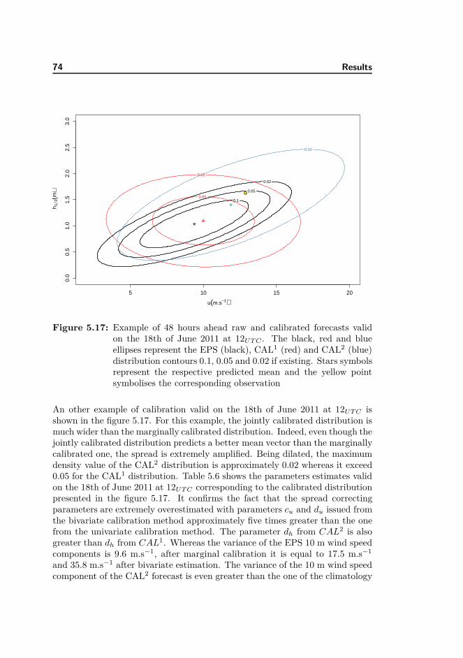
74 Results
u(m.s−1)
h 13(m
)
0.1
0.05
0.02
5 10 15 20
0.0
0.5
1.0
1.5
2.0
2.5
3.0
0.05
0.02
0.02
Figure 5.17: Example of 48 hours ahead raw and calibrated forecasts validon the 18th of June 2011 at 12UT C . The black, red and blueellipses represent the EPS (black), CAL1 (red) and CAL2 (blue)distribution contours 0.1, 0.05 and 0.02 if existing. Stars symbolsrepresent the respective predicted mean and the yellow pointsymbolises the corresponding observation
An other example of calibration valid on the 18th of June 2011 at 12UT C isshown in the figure 5.17. For this example, the jointly calibrated distribution ismuch wider than the marginally calibrated distribution. Indeed, even though thejointly calibrated distribution predicts a better mean vector than the marginallycalibrated one, the spread is extremely amplified. Being dilated, the maximumdensity value of the CAL2 distribution is approximately 0.02 whereas it exceed0.05 for the CAL1 distribution. Table 5.6 shows the parameters estimates validon the 18th of June 2011 at 12UT C corresponding to the calibrated distributionpresented in the figure 5.17. It confirms the fact that the spread correctingparameters are extremely overestimated with parameters cu and du issued fromthe bivariate calibration method approximately five times greater than the onefrom the univariate calibration method. The parameter dh from CAL2 is alsogreater than dh from CAL1. Whereas the variance of the EPS 10 m wind speedcomponents is 9.6 m.s−1, after marginal calibration it is equal to 17.5 m.s−1
and 35.8 m.s−1 after bivariate estimation. The variance of the 10 m wind speedcomponent of the CAL2 forecast is even greater than the one of the climatology

5.3 Bivariate calibration method 75
Method au bu cu du ah bh ch dh
CAL1 0.09 1.03 0.65 1.85 0.07 0.97 0.00 2.42CAL2 -0.49 1.09 3.28 5.20 0.02 1.07 0.00 7.53
Table 5.6: Example of parameters estimates of the bivariate and univariatecalibration method for 48 hours ahead the wind speed (au,bu,cu,du)and the wave height forecasts (ah,bh,ch,dh) valid on the 18th of June2011 at 12UT C (issued the 16th of September 2011 at 12UT C).
forecast. In consideration of the previous example, it seems that the maximumlikelihood estimation technique is not as efficient for the bivariate approach asfor the univariate.
The corresponding EPS and CAL2 distributions are illustrated in three-dimensionin figure 5.18. The spread parameters overestimation can clearly be seen. In-deed, even if the mean correction is correct leading to a very well predictedmean, the distribution is way too wide, tails in the wind speed components goeseven beyond 20m.s−1. The maximum of the pdf is approximately 0.04 which isvery low compared to the pdf of the EPS (0.2).

76 Results
u
0
5
10
15
20
h
0
2
4
6
8
PD
F
0.00
0.05
0.10
0.15
0.20
(a) EPSu
0
5
10
15
20
h
0
2
4
6
8
PD
F
0.00
0.01
0.02
0.03
0.04
(b) CAL2
Figure 5.18: Example of three diemnsional 48 hours ahead (a) raw and (b)jointly calibrated forecasts distribution valid on the 18th of June2011 2011 at 12UT C . The yellow point the corresponding obser-vation

5.3 Bivariate calibration method 77
Days of the training period
Indi
vidu
al li
kelih
ood
func
tion
−15
000
−10
000
−50
000
without correlationwith correlation
Figure 5.19: Truncated bivariate normal logarithm density values of the dif-ferent observations introduced in the training period for the bi-variate calibration valid on the 18th of June 2011 at 12UT C . Theblack bars are valid when the correlation is null whereas the or-ange bars are valid for a correlation equal to the EPS correlation.
Figure 5.19 shows logarithm density values (symbolised by bars) corresponding
to the pairs observation - predicted distribution (xi, fi) present in the trainingperiod for the bivariate calibration valid on the 18th of June 2011 at 12UT C . Log-arithm density are identical to individual log-likelihood function and thereforeinform about the respective contribution of the different pairs for the parameterestimation on the valid date. The black bars are the density values (equation(4.16)) with a correlation equal to zero and the orange bars are density valueswith a correlation equal to the predicted correlation. It can be noticed that tak-ing into account the correlation strongly impacts the density values. Indeed, thevalues range is strongly increased with maximum at -20000 instead of approxi-mately -8000. Most of the density values are increased apart from some eventslike the third from the left or the sixth from the right where it is decreased.It seems that taking into account the predicted correlation gives more weighton outliers resulting in an overestimation of the spread correcting parameterscompared to the univariate approach (see Table 5.5).
Figure 5.20 shows more precisely one of the outliers seen in the figure 5.19,corresponding to the 48 hours ahead forecasts valid on the 8th of May 2011 at

78 Results
u
6
8
10
12
14
h
1.0
1.5
2.0
2.5
3.0
PD
F
0
1
2
3
Figure 5.20: Outlier observation of the 8th of May 2011 at 12UT C introducedin the training period for the calibration valid on the 18th ofJune 2011 at 12UT C with the corresponding raw forecasts withthe predicted correlation (black) and with a correlation equal tozero (grey)
12UT C . The corresponding predictive raw bivariate distribution which a non nullcorrelation is represented in three dimensions and the corresponding observationis symbolised by the yellow point. The prediction for that day can be consideredas bad, that is the predicted mean is far from the observation and the predictivedistribution is way too sharp. Thus, the individual log-likelihood function ofthis observations is strongly negative. The fact that for this event, the obser-vation lies on the orthogonal direction of the bivariate distribution preferentialdirection strongly impacts the respective log-likelihood function, that is makesit much lower. Indeed, the figure 5.19 shows that the individual log-likelihoodvalue of this observation (thirteenth from the left of the figure) is approximately-15000 whereas it is around -2500 when the predicted correlation is considered

5.3 Bivariate calibration method 79
as zero.Here we want to point out an issue encountered by the bivariate calibrationmethod. An observation is considered as an outlier when it falls far from theensemble distribution. However, taking the predicted correlation into accountas it is done by the bivariate calibration method proposed here tends to sharperpredicted distributions and can amplify the outlier characteristic of an observa-tion and therefore enhance his weight during the parameter estimation process.
Figure 5.21 shows the evolution of the estimated parameters au, bu, cu, du, ah,bh, ch and dh for the different 48 hours ahead wind speed and the significantwave height forecast calibration methods over the entire period from January2010 to December 2011. The marginally estimated parameters are representedin black whereas the jointly estimated parameters are represented in red. Wecan see that the mean correcting parameters a and b evolve anti-symmetrically,that is a becomes larger when b becomes smaller b and vice versa. We can noticethat in general, corrections are smaller for the significant wave height forecaststhan for the 10m wind speed, ah amplitudes is approximatively 0.4 whereas au
take values from -3 to +1. It is even stronger for the variance correcting pa-rameters cu and ch. Indeed, ch’s order of magnitude is more than twenty timessmaller than for cu. The parameters au and bu tend to be closer to 0 and 1during the year 2011. Indeed, as it can be noticed in figure 5.8, the bias of theyear 2011 is very close to zero contrary to the year 2010, thus the correction ofthe location parameter is much less important during the second year data.Parameters estimated from the bivariate and the univariate calibration methodmainly differ from the spread parameters. Parameters au,bu, ah,and bh are verysimilar, their difference might only be due to the difference of the training pe-riod. Indeed, we remind that, unlike for the univariate calibration method, both10 m wind speed and significant wave height have to available to be introducedin the training period of the bivariate calibration method. Parameters cu,du,ch,and dh are very different from one method to the other. The one estimatedthrough the bivariate calibration method are always greater than the othersand seem to be strongly overestimated at some point. Whatever the parameter,short oscillations can be seen, result of the small length of the training periodallowing a faster adaptation to forecast errors variations.
Figure 5.22 compares once again the marginally estimated parameters (repre-sented in black) with parameters estimated through a bivariate approach whilefixing the correlation to zero (represented in green). The two method presentsimilar results with slight differences mainly due to the training period usedfor the estimation. This figure confirms the fact that the overestimation of thespread correcting parameters is not due to the use of a bivariate distributionbut essentially to the fact that a non null correlation is provided. Indeed, taking

80 Results
into account the correlation tends to sharper distributions that might have tobe strongly dilated to cover observations lying on the orthogonal direction tothe one impose by the correlation prescribed by the EPS.

5.3
Biv
aria
tecalib
ratio
nm
eth
od
81
0 200 400 600
−3
−2
−1
01
Daily Index
a u
0 200 400 6000.
70.
80.
91.
01.
11.
21.
3
Daily Index
b u0 200 400 600
02
46
810
1214
Daily Index
c u
0 200 400 600
02
46
810
12
Daily Index
d u
0 200 400 600
−0.
20.
00.
20.
4
Daily Index
a h
0 200 400 600
0.7
0.8
0.9
1.0
1.1
1.2
1.3
Daily Index
b h
0 200 400 600
0.00
0.05
0.10
0.15
0.20
0.25
Daily Index
c h
0 200 400 600
02
46
8
Daily Index
d h
Figure 5.21: Parameter estimates au,bu,cu and du (from left to right) for the 10m wind speed (top) and ah,bh,ch and dh
for the significant wave height (bottom) for the 48 hours ahead univariate calibration CAL1 (black) andbivariate calibration CAL2 (red) from January 2010 to December 2011
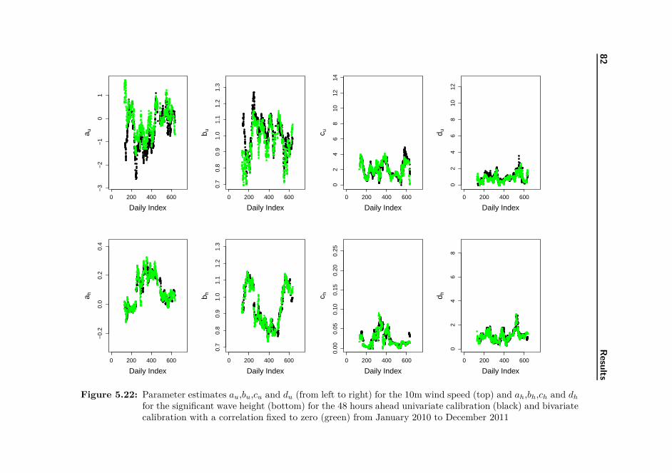
82
Resu
lts
0 200 400 600
−3
−2
−1
01
Daily Index
a u
0 200 400 600
0.7
0.8
0.9
1.0
1.1
1.2
1.3
Daily Indexb u
0 200 400 600
02
46
810
1214
Daily Index
c u
0 200 400 600
02
46
810
12
Daily Index
d u
0 200 400 600
−0.
20.
00.
20.
4
Daily Index
a h
0 200 400 600
0.7
0.8
0.9
1.0
1.1
1.2
1.3
Daily Index
b h
0 200 400 600
0.00
0.05
0.10
0.15
0.20
0.25
Daily Index
c h
0 200 400 600
02
46
8
Daily Index
d h
Figure 5.22: Parameter estimates au,bu,cu and du (from left to right) for the 10m wind speed (top) and ah,bh,ch and dh
for the significant wave height (bottom) for the 48 hours ahead univariate calibration (black) and bivariatecalibration with a correlation fixed to zero (green) from January 2010 to December 2011

5.3 Bivariate calibration method 83
0.00
0.01
0.02
0.03
Fre
quen
cy
Figure 5.23: Multivariate rank histogram of the 48 hours ahead CAL2 fore-casts of 10m wind speed and significant wave height.
Figures 5.23 shows the multivariate rank histograms of the jointly calibratedforecasts CAL2. As it has been noticed previously with the example given inthe figure 5.15, the jointly calibrated forecasts CAL2 are clearly overdispersive.This is the result of overestimations of the spread correcting parameters cu, du,ch and dh.
Calibration Method bRMSE bMAE es ∆ DS
EPS 1.998 1.752 1.179 0.481 0.355Climatology 3.724 3.594 2.078 0.064 1.468
CAL1 1.971 1.729 1.110 0.094 0.699CAL1+ 1.973 1.733 1.114 0.229 0.51CAL2 2.116 1.864 1.212 0.468 0.768
Table 5.7: Comparison of bivariate scores of the different calibration methodsfor the +48h forecasts over the entire period
Table 5.7 presents bivariate scores of every forecasts types studied in this thesisfor the 48 hours prediction horizon. Since results of the first forecast types havealready be discussed previously, we only focus here on the bivariate calibrationapproach CAL2. Obviously, the bivariate approach jointly calibrating the fore-casts CAL2 presents bad results. Since forecasts sample a truncated bivariatenormal distribution, even if the mean correcting parameters are similar to theCAL1 method, the overestimation of the spread parameters impacts the ensem-ble mean. Indeed, the mean of the truncated normal distribution is affected by

84 Results
the variance. (see equation (4.4)). Thus, the bRMSE of the CAL2 forecasts iseven worse than for the raw forecasts. It is also true for the bMAE and theenergy score. Even if the Reliability index is slightly improve compared to theEPS, the forecasts are strongly overdispersive and present the less sharp cali-brated forecasts.Unfortunately, even if the bivariate approach is promising, the maximum likeli-hood technique appears to be too sensitive too outliers which is the reason whythe method is therefore not efficient.

Chapter 6
Discussion
As explained in the introduction, wind and wave ensemble forecasts are of agreat interest for a number of decision-making problems. They inform aboutthe possible future states of the atmosphere and are of substantial economicvalue. However, ensemble forecasts tend to be uncalibrated, that is biasedand underdispersive. Statistical post-processing methods are used to improvepredictive performance while providing reliable probabilistic forecasts. So farthese calibration methods mainly deal with univariate ensemble forecasts andtherefore do not take into account any possible correlation of two-dimensional(or more) forecasts. We proposed a bivariate approach jointly calibrating 10m wind speed and significant wave height ensemble forecasts so that essentialbivariate characteristics can be captured.
Empirical analysis showed that 10 m wind speed and significant wave heightcould be modelled by a truncated bivariate normal distribution with a cut-offat zero for both variables. The mean vector and the variances of the underly-ing normal distribution are respectively assumed to be a linear function of thepredicted mean vector and variances. The optimal correcting parameters aresimultaneously estimated by maximum likelihood estimation on a sliding win-dow of 42 days. A method using the raw predicted correlation to recover thedependence lost during the marginal calibration is also tested. Bivariate distri-bution provided by this method share the same univariate properties than themarginally calibrated distribution, though they additionally have an informative

86 Discussion
correlation.
The univariate calibration method CAL1 has proved to be the most efficientsince considerably increasing reliability of raw forecasts while reducing bRMSEof almost 6% and the energy score of approximately 20% for the first predic-tion horizons. However this technique does not take into account the existingrelationship between the two variables and therefore predicts uncorrelated dis-tributions. The EPS-prescribed correlation approach CAL1+ does not presentbetter improvements than the univariate approach as well. Even if calibratedforecasts seem more realistic and are sharper, forecasts are less reliable and theenergy score is worsened. These results prove that a bivariate approach jointlycalibrating forecasts is needed. Yet, the proposed bivariate calibration methodCAL2 does not appear to be efficient. Indeed, the likelihood technique is toosensitive to outliers when the correlation is taken into account and yields anoverestimation of the spread correcting parameters. Calibrated forecasts aretherefore overdispersive resulting in worse bivariate scores. Outliers falling onthe orthogonal direction as the one imposed by the correlation are the cause ofthe spread parameters overestimation.
We have seen that enlarging the training period is not a sufficient solution tosolve the overestimation issue. Therefore, two options can be envisaged: the firstone would be to model 10 m wind speed and significant wave height with a dis-tribution having heavier tails than the truncated bivariate normal distribution.The second option would be to use of a robust maximum likelihood technique.These two perspectives could permit to reduce the problem introduced by theseso-called outliers.
Furthermore in this thesis, it was always assumed that the predicted correlationof the EPS were exact. Though, the correlation might be incorrect and evenshow systematic errors. Once the maximum likelihood technique sensitivityissue solved, it would be interesting to investigate a possible correction of theraw predicted correlation. A linear correction had been envisaged,
ρt+k = e+ fρt+k|t
The parameters e and f would be estimated during the training period. How-ever, since the correlation parameter ρ ∈ {−1; 1}, these parameters have thento be constrained so the corrected correlation would also be defined on the sameinterval. In order to ensure that condition, we could write,
ρt+k = cos ε+ (1 − | cos ε|) cos ζρt+k|t

Appendix A
List of Notations

88 List of Notations
x Observation vectorxu Observed 10 m wind speedxh Observed significant wave heightµ true meanσ2 true varianceρ true correlationy(j) jth ensemble member
f predictive probability density function
F predictive cumulative density functionµ predictive mean vectorµu predictive mean 10 m wind speedµh predictive mean significant wave heightyu ensemble mean 10 m wind speedyh ensemble mean significant wave height
Σ predictive variance-covariance matrixσ2
u predictive variance for 10 m wind speedσ2
h predictive variance for significant wave heights2
u ensemble variance for 10 m wind speeds2
u ensemble variance for significant wave heightyu ensemble median for 10 m wind speedyh ensemble median for significant wave heightM number of ensemble membersn length of the training periodt issued data of the forecastt+ k valid date of the observation/forecastk lead timeI(condition) Indicator function equal to 1 if condition is true 0 otherwise

Bibliography
Baars, J. (2005). Observations qc summary page.http://www.atmos.washington.edu/mm5rt/qc_obs/qc_obs_stats.html.
Bidlot, J. and Holt, M. (1999). Numerical wave modelling at operational weathercentres. Coastal Engineering, 37:409–429.
Bröcker, J. and Smith, L. (2008). From ensemble forecasts to predicitve distri-bution functions. Tellus A, 60:663–678.
Charnock, H. (1995). Wind stress on a water surface. Quarterly Journal of the
Royal Meteorological Society, 81:639–640.
Delle Monache, L., Hacker, J., Zhou, Y., Deng, X., and Stull, R. (2006). Proba-bilistic aspects of meteorological and ozone regional ensemble forecasts. Jour-
nal of Geophysical Research, 111:1–15.
Gneiting, T. (2011). Quantiles as otpimal point forecasts. International Journal
of Forecasting, 27:197–207.
Gneiting, T., Balabdaoui, F., and Raftery, A. (2007). Probabilistic forecasts,calibration and sharpness. Quarterly Journal of the Royal Meteorological So-
ciety, 69:243–268.
Gneiting, T. and Raftery, A. (2007). Strictly proper scoring rules, predictionand estimation. Journal of the American Statistical Association, 102:359–378.
Gneiting, T., Raftery, A., Westveld III, A., and Goldman, T. (2005). Calibratedprobabilistic forecasting using ensembe model output statistics and minimumcrps estimation. Monthly Weather Review, 133:1098–1118.

90 BIBLIOGRAPHY
Gneiting, T., Stanberry, L., Grimit, E., Held, L., and Johnson, N. (2008). As-sessing probabilistic forecasts of multivariate quantites, with an applicationto ensemble predictions of surface winds. Technical Report 537, Departmentof Statistics, University of Washington.
Hinnenthal, J. (2008). Robust Pareto – Optimum Routing of Ships utilizing De-
terministic and Ensemble Weather Forecasts. PhD thesis, Technical UniversityBerlin.
Horrace, W. (2005). Some results on the mutlivariate truncated normal distri-bution. Journal of Mutlivariate Analysis, 94:209–201.
Mathiesen, B., Lund, H., and Karlsson, K. (2009). The ida climate plan 2050,background report. Technical report, Aalborg University,RIS∅-DTU.
Möller, A., Lenkoski, A., and Thorarinsdottir, T. (2012). Multivari-ate probabilistic forecasting using bayesian model averaging and copulas.arXiv:1202.3956v1.
Murphy, A. (1993). What is a good forecast? an essay on the nature of godnessin weather forecasting. Monthly Weather Review, 8:281—-293.
Pawitan, Y. (2001). In all likelihood : Statistical modelling and inference using
likelihood. Oxford Science Publication.
Pinson, P. (2012). Adaptative calibration of (u,v)- wind ensemble forecasts.Quarterly Journal of the Royal Meteorological Society, 138(666):1273–1284.
Pinson, P. and Hagedorn, R. (2012). Verification of the ecmwf ensemble forecastsof wind speed against analyses and observations. Meteorological Application,00:1–20.
Pinson, P., Nielsen, H., Moller, J., and Madsen, H. (2007). Nonparametricprobabilistic forecasts of wind power: required properties and evaluation.Wind Energy, 10:497–516.
Pinson, P., Reikard, G., and Bidlot, J. (2012). Probabilistic forecasting of thewave energy flux. Applied Energy, 93:364–370.
Raftery, A., Gneiting, T., Balabdaoui, F., and Polakowski, M. (2005). Usingbayesian model averaging to calibrate forecast ensembles. Monthly Weather
Review, 133:1155–1174.
Schuhen, N., Thorarinsdottir, T., and Gneiting, T. (2012). Ensemble modeloutput statistics for wind vectors. Monthly Weather Review, In Press.
Sloughter, J., Gneiting, T., and Raftery, E. (2010). Probabilistic wind speedforecasting using ensembles and bayestian model averaging. Journal of the
American Statistical Association, 105:25–35.

BIBLIOGRAPHY 91
Tambke, J., Bye, J., Wolff, J., Tautz, S., Lange, B., Lange, M., and Focken, U.(2004). Modelling offshore wind profiles using inertially coupled wave bound-ary layers. In Proceedings of the 2004 European Wind Energy Conference.
Thorarinsdottir, T. and Gneiting, T. (2008). Probabilistic forecast of windspeed: Ensemble model output statistics unsing hereoskedastic censored re-gression. Technical Report 546, Deparment of Statistics, University of Wash-ington.
Wilhelm, S. and Manjunath, B. (2010). tmvtnorm: A package for the truncatedmutlivariate normal distribution. The R Journal, 2(1):25–29.
Wilks, D. (2006). Statistical Methods in the Atmospheric Sciences, 2nd edition.Academic Press.
Wilks, D. and Hamill, T. (2007). Comparison of ensemble-mos methods usinggfs reforecasts. Monthly Weather Review, 135:2379–2390.