Wind Pressure Coefficients on Pyramidal Roof of Square ...

Computational Engineering and Physical Modeling 1-1 (2019) 01-16

How to cite this article: Singh J, Roy AK. Wind Pressure Coefficients on Pyramidal Roof of Square Plan Low Rise Double Storey

Building. Comput Eng Phys Model 2019;2(1):1–16. https://doi.org/10.22115/cepm.2019.144599.1043

2588-6959/ © 2019 The Authors. Published by Pouyan Press.

This is an open access article under the CC BY license (http://creativecommons.org/licenses/by/4.0/).

Contents lists available at CEPM

Computational Engineering and Physical Modeling

Journal homepage: www.jcepm.com

Wind Pressure Coefficients on Pyramidal Roof of Square Plan

Low Rise Double Storey Building

J. Singh1* , A.K. Roy2

1. Ph.D., Scholar, Department of Civil Engineering, National Institute of Technology Hamirpur, Himachal Pradesh

177005, India

2. Assistant Professor, Department of Civil Engineering, National Institute of Technology Hamirpur, Himachal

Pradesh-177005, India

Corresponding author: [email protected]

https://doi.org/10.22115/CEPM.2019.144599.1043

ARTICLE INFO

ABSTRACT

Article history:

Received: 17 August 2018

Revised: 26 January 2019

Accepted: 10 April 2019

The present study demonstrates the pressure variation due to

wind load on a two storey building with a square plan and a

pyramidal roof through CFD simulation. Past cyclone reports

and other related post-disaster studies have shown loss of lives

and extensive property loss mostly in the cyclone prone regions

of India. Post-disaster studies reveal that a pyramidal roof has

much better chances of survival in comparison with other roof

shapes. ANSYS Fluent has been used for the simulation and

ANSYS CFD-Post has been used for observing the wind

pressure on building roofs. The simulations are performed using

the realizable k-ε turbulent model by considering grid sensitive

analysis and validation with previously published wind tunnel

experminetal measurements. The present study includes wind

behaviour around the building model with different roof slopes.

Comparisons of pressure coefficients are shown for five wind

incidence angles to study the effect of wind on the building.

Results indicate that both maximum positive and maximum

negative wind pressure coeffiecients increase with increasing

roof slopes. The results of the study is helpful in understanding

the damage caused on the roof surface during the extreme wind

condition.

Keywords:

Computational fluid dynamics;

Pressure coefficients;

Pyramidal building model;

Roof slope;

Wind incidence angle.


https://doi.org/10.22115/cepm.2019.144599.1043

http://creativecommons.org/licenses/by/4.0/

http://www.jcepm.com/

mailto:[email protected]


https://www.orcid.org/0000000291216581

https://www.orcid.org/0000-0003-2439-4086

2 J. Singh, A.K. Roy/Computational Engineering and Physical Modeling 2-1 (2019) 01-16

1. Introduction

The roofed buildings are widely used in coastal areas of India as well as all around the world.

These roofed buildings are exposed to the atmospheric wind speed experiencing significant wind

loads on the roof structures. In old-fashioned roofing systems, high wind-induced suctions can

cause major damage which can lead to subsequent rain intrusion and loss of interior substances

[1]. Initial damage due to extreme winds is the destruction of cladding, which can be often seen

as the beginning of structure failure and inhabitant injury during a dangerous wind occurrence

[2]. Thus for the structure’s design, along with other loads, wind load should also be considered.

Wind tunnel testing is one of the ways to investigate structures for wind loading. But this is a

time consuming and expensive process and requires a lot of effort.

As an alternative to wind tunnel testing, CFD simulation[3–5] is used nowadays to determine the

effects of wind on structures [6]. In computational fluid dynamics, i.e. CFD, numerical analysis

is utilized to find solutions to various problems involving fluid flows[7,8]. In this branch of fluid

mechanics, computers are used for the calculations necessary to simulate the free-stream flow of

the fluid as well as the surface interaction of the fluid as defined by boundary conditions [9].

Thus, CFD may be defined as the use of applied mathematics, physics and computational

software that is used to evaluate fluid flow behavior. It is based on the Navier-Stokes equations,

which show how the velocity, pressure, temperature, and density of a moving fluid are

interrelated [10]. CFD reduces both time and cost in design and research, and provides detailed

and visualized information [11]. Lots of computational work carried out by numbers of

researchers using ANSYS Fluent [8,12–16]. This software is novice friendly while remaining

highly accurate and quick [9]. A fair number of studies have been carried out through CFD

simulation instead of wind tunnel testing and have shown that the results for velocity profiles

near test sections obtained from CFD simulations are almost identical to experimental results

[17].

CFD simulations also have been used for testing different aerodynamic mitigation techniques

[18]. As CFD simulation is multifunctional and a useful tool, it has proven very effective to

evaluate the unsteady aerodynamic forces on the vibrating roof in a wider reduced frequency

range [19]. The pressure values at various locations (variation of pressure with respect to

locations on a building structure), flow streamline (paths of flow particles which show the eddies

and vortices), velocity vector (these shows both the velocity magnitude and movements of

velocity streamlines) and characteristics of numbers of related constraint variables etc. can be

observed and assessed with the help of CFD study [16]. Ozmen et al. [20] carried out

experimental and numerical studies of turbulent flow fields on gabled roofed low-rise building

models with different pitch angles immersed in atmospheric boundary layer using realizable k-ε

turbulence model which exhibit a good agreement with regard to predicting mean velocity and

turbulence kinetic energy while standard k-ω turbulence models also show accuracy with regard

to predicting mean pressure coefficients.

https://en.wikipedia.org/wiki/Boundary_value_problem#Boundary_value_conditions

J. Singh, A.K. Roy/Computational Engineering and Physical Modeling 2-1 (2019) 01-16 3

Wind direction also has a noticeable effect on pressure magnitude. In a wind tunnel study, it was

found that changes in the wind incidence angle may induce dissimilar pressures on different

surfaces of a ‘+’ plan shaped structure [21]. In a study of wind loads on roof tiles, vulnerability

analysis indicated that applying the net wind uplift loading on tiles rather than external surface

pressures only gives rise to roof tile damage [22]. A full-scale wind testing facility, generically

known as Wall of Wind (WOW), has been used to investigate wind-induced internal and external

pressures and pressure coefficients on the eaves of hip roofs and gable roofs. It was found that

these coefficients were lower for the former i.e. hip roofs [23]. As the pressure or suction vary

with the shape and size of structure and its roof, the highest suction was found near the corner

edges and near ridgeline of roof in case of a canopy roof [24], and this type of roof was also

found more vulnerable to windstorms as compare to other types of roofs [25].

Different countries have their wind codes for evaluating wind loads like Indian wind code IS 875

(Part 3)[26], Australian wind code AS/NZS 1170.2:2011[27] and American wind code

ASCE/SEI: 7-10, [28] etc. In these codal provisions includes the pressure coefficients on gable

roof, multi-span gable roof, hip roof, canopy roof, saw tooth roof, and mono slope roof. None of

the code have information on pyramidal roof buildings with different height.

In experimental and numerical investigations of flat, conical and hemispherical roof models, the

hemispherical roof was found to have the most critical pressure field and a good agreement was

seen between experimental and numerical outcomes [29,30] [31]. This review of literature shows

that most of the studies till date are on low rise buildings with gable roof, multi-span gable roof,

hip roof, canopy roof, saw tooth roof, mono slope roof and dome shaped roofs. No studies have

been conducted on pyramidal roof buildings with different height.

Therefore, in this paper, the impact of the roof inclination angle on pyramidal roof of low rise

buildings is analyzed using Computational Fluid Dynamics (CFD). A CFD analysis is required

for this study since the performance assessment of the different roof geometries is not only based

on the inclination of the roof surface and wind direction, but also on the airflow pattern

(velocities) around the building resulting from different vertical exposed area. In the past 50

years, CFD has evolved into a powerful tool for research works in urban physics and building

aerodynamics [32]. In this paper, the simulations are performed using realizable k-ε turbulent model by

considering grid sensitive analysis and validation with previously published wind tunnel

experimental measurements. The detailed analysis of the airflow performing CFD simulation are

modeled simultaneously in the same computational domain. The detailed wind-tunnel velocity

and turbulence intensity measurements provided by David et al. [27] for the wind tunnel study on

wind loads on gable roof building with interference of boundary wall and a flat roof are used for

model validation.

First, the wind tunnel experimental data used in present study is described in Section 2. Then, the

setting of computational domain and parameters are presented in Section 3 and the validation of

results in Section 4, after which the pressure variation on roof and velocity around building

models are outlined in Section 5 and a comparison with codal values is also carried out in the

same section. Finally section 6 presents the conclusion of the study.


2. Wind tunnel Experimental data used

David et al. [33] carried out wind tunnel tests in an open circuit atmospheric boundary layer

wind tunnel at the Indian Institute of technology Roorkee (India). The wind tunnel has a cross

section 2.1m x 2.0m with a test section of 15m length and the wind speed of 18m/s can be

achieved in this wind tunnel. In his study mean velocity and longitudinal turbulence intensity

profiles for terrain category simulated in the wind tunnel have been used for the CFD simulation

and validated.

In our study the velocity profile has a power law exponent (α = 0.14) and the values of mean

velocity and longitudinal turbulence intensity at the eave height (H) of the model have been

found to be 8 m/s and 18% respectively. The longitudinal length scale of turbulence Lux, was

determined by calculating area under the autocorrelation curve of the fluctuating velocity

component and at a height H of 195 mm, Lux is about 0.45 m which is approximately 45 m as the

equivalent full-scale Lux.

3. CFD simulation: setting of computational domain and parameters

The computational settings and parameters for the present study are described in this section.

These settings and parameters has been used for the sensitivity analyses (grid resolution,

turbulence model, inlet turbulent kinetic energy), which has been presented in Section 4.

3.1. Computational domain and grid

In our study the computational domain and grid are constructed at reduced scale (1:25) to exactly

resemble the wind-tunnel geometry as mentioned in the section 2. The building model in Figure

1 and computational domain Figure 2 adhere to the best practice guidelines by Franke et al. [34]

and Revuz et al. [15]. The dimensions of the domain are 2.725×5.225×1.5 m3 (W×D×H) which

correspond to 68.125×130.625×37.5 m3 in full scale. The computational grid is fully structured

and created using the surface grid extrusion technique which is described by van Hooff and

Blocken [35]. The maximum stretching ratio is 1.2 and the first cell height is 4 mm at the

building wall. A grid-sensitivity analysis is performed based on three grids, coarse, basic and fine

grid and the results of the grid-sensitivity analysis are incorporated. The basic grid is a suitable

grid for this study shown in Figure 3 and this grid is used in all the CFD simulations carried out.

Ansys ICEM CFD tool is used to produces advanced geometry/mesh generation and mesh

diagnostics and repair functions, which are required for flow analysis. An additional advantage

of ICEM CFD is that it can create its own geometry or import geometry via external CAD

software. In this study, since our structure design was relatively simple, we have created

geometry using ICEM CFD [36]. A two Storey building model with a pyramidal roof was created

in ICEM CFD. The base area of the building model is identical to the one in the study carried out

at the Central Building Research Institute, Roorkee (India) [37]. Measurements were conducted

at the scale of 1:25. The dimensions of the base of the building model and domain geometry is

shown in Figure 1 and Figure 2 respectively. Once the domain for the model was defined, the

next step was to create the geometry of the building model within domain in ICEM CFD.


Fig. 1. Dimensions of building model(a. side view and b. plan).

Fig. 2. CFD Domain for the building simulation.

For simulation work, it is necessary to distribute the whole domain volume into small cells also

known as meshing. A hexahedral type of mesh is simple to generate and also gives good results.

So a structured hexahedral grid was used for meshing. The mesh was created with refined grid

near the model as shown in Figure 3 for getting more accurate results.

For good results and a simpler simulation process, the mesh quality should be more than 0.5,

which is considered good. Quality of mesh should be checked for every model. The quality of

mesh was above 0.6 in each model. The mesh quality can be checked on a scale of 0.0 to 1.0 in

ICEM CFD as can be seen in Figure 3(right lower side). The bottom right part of Figure shows a

bar chart for quality check, while the bottom left part of Figure shows the quality criterion i.e.

number of cells under different quality criterion. After the quality check, the mesh was converted

into unstructured mesh, since Ansys Fluent was used for simulation work in the present study

and it supports only unstructured mesh.


Fig. 3. Meshing of domain and building model.

3.2. Boundary condition

For the real physical demonstration of the fluid flow, appropriate boundary conditions that really

simulate the actual flow are necessary. Defining the detail boundary conditions at the inlet and

outlet of the flow domain, which is essential for a precise solution, is always problematic. With

the following expressions for the along wind component of velocity, a velocity inlet was used at

the windward boundary. The mean velocity, U is similar to the experimental study. Standard

depiction of the velocity profile in the ABL is as shown below.

U(z)u∗

κ= ln (

z+z0

z0) (1)

The velocity profile and turbulence intensity profile is used from the experimental study by John

et al. [38] carried out in the wind tunnel at IIT Roorkee. It seems necessary to validate the

numerical results with the help of experimental results and for this purpose validation of velocity

profile and turbulence intensity has been shown in Figure 4.

y = 1.0559ln(x) + 2.3323

R² = 0.9764

0

2

4

6

8

10

12

0 200 400 600 800 1000

Vel

(m

/s)

Height (cm)

Wind Tunnel Velocity

Trendline (Log)


Fig. 4. Experimental results for velocity profile and turbulence intensity [38].

From Figure 4, it can be seen that the wind tunnel velocity profile representing the trend line

with the equation y=1.0559ln(x)+4.7636 and the turbulence intensity profile representing the

trend line with the equation y=0.7554x-0.297 is used as User defined function (UDF) at the inlet

boundary to generate the boundary layer flow throughout the domain. The top and the sides of

the computational domain are displayed as slip walls (zero normal velocity and zero normal

gradients of all variables). At the outlet, zero static pressure is stated.

3.3. Solver settings

The finite-volume method in ANSYS Fluent is used for solving governing equations and

associated problem-specific boundary conditions. The basic principle of using finite element

method is that the body is sub divided into small isolated areas known as finite elements. Size of

the stiffness matrix be determined by only the number of nodes and the results are amended by

increasing the number of nodes and collocation points [39]. Each element has governing

equations in Fluent & these elements are accumulated into a global matrix.

As stated in previously the solutions were steady-state. Second-order differencing was used for

the momentum, pressure and turbulence equations and the “coupled” pressure-velocity coupling

method due to its robustness for steady-state, single-phase flow problems.

The residuals fell below the generally applied criteria of falling to 10-4 of their initial values after

more than a few hundred iterations. The drag, lift and side forces and the moments subjected to

the pyramidal roof building were examined during the simulation and only when they attained

stationary values the simulations considered to have converged. Although the simulations were

steady-state, there was some variation (< 1%) in the “steady” values of the various monitoring

values.

y = 0.7554x-0.297

R² = 0.9143

0

0.05

0.1

0.15

0.2

0.25

0.3

0.35

0 200 400 600 800 1000

Lo

ngit

ud

inal

Turb

uil

ence

Inte

nsi

ty (

I)

Height (mm)

Wind Tunnel T.I.

Trendline (Power )


4. CFD simulation: Validation

First, geometrical models of five pyramidal building types with roof slopes of 20°, 25°, 30°, 35°

and 40° were created in ICEM CFD. Then a good mesh quality was achieved, and subsequently

simulation of all models was performed in Ansys Fluent. For simulation, Realizable k-epsilon

method was used. In the present study, since the velocity profile was taken from atmospheric

boundary layer wind tunnel results, it increases with increasing height as shown in Figure 5.

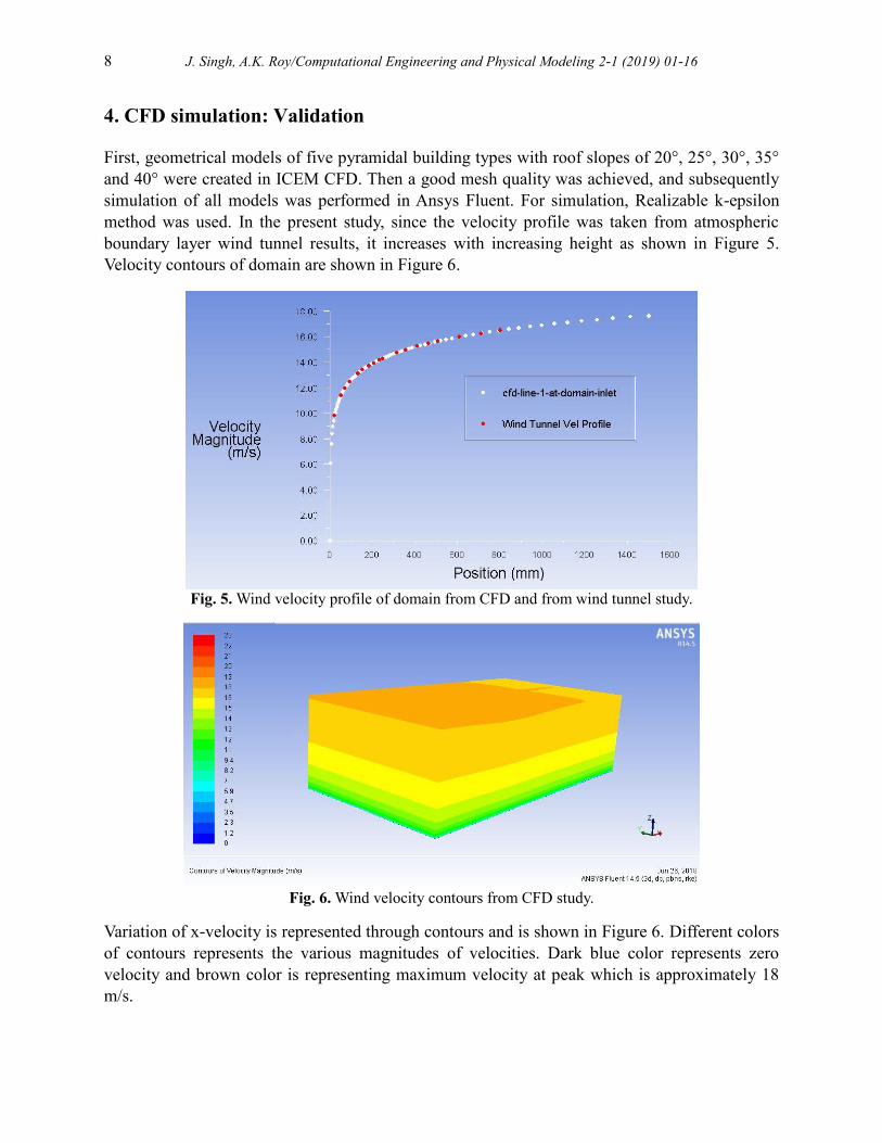
Velocity contours of domain are shown in Figure 6.

Fig. 5. Wind velocity profile of domain from CFD and from wind tunnel study.

Fig. 6. Wind velocity contours from CFD study.

Variation of x-velocity is represented through contours and is shown in Figure 6. Different colors

of contours represents the various magnitudes of velocities. Dark blue color represents zero

velocity and brown color is representing maximum velocity at peak which is approximately 18

m/s.


5. Discussion

5.1. Pressure coefficients on the building roofs

The Wind pressure coefficient is a dimensionless number that defines how the pressure is

different from the static pressure in proportion to the dynamic pressure. If the pressure is more

than the static pressure, then the coefficient is positive and if the pressure is less than the static

pressure, then the coefficient is negative. Contours of wind pressure coefficients were generated

in Fluent for five roof slopes all with 0° wind incidence angle and are shown in Figure 7.

Fig. 7. Contours of Pressure Coefficients on roof of Pyramidal building models with roof slopes of (a)

20°, (b) 25°, (c) 30°, (d) 35°, (e) 40° with 0° wind incidence angle. (continued…).

Fig. 7. Contours of Pressure Coefficients on roof of Pyramidal building models with roof slopes of (a)

20°, (b) 25°, (c) 30°, (d) 35°, (e) 40° with 0° wind incidence angle. (continued…).


In Figure 7, the blue regions represent areas of greatest negative pressure, the green color shows

regions of lower negative pressure, yellow shows neutral, while increasing positive pressure

zones are shown as orange and red.

For the model with a 20° slope, the edges of the windward surface show the highest negative

pressure (suction) (Cp= -1.4) while the remaining roof surfaces show lower negative pressures.

For this roof slope, there are no areas of positive pressure. For the 25° slope, the maximum

suction (Cp= -2.1) is seen on the ridgeline. For this slope as well there are no areas of positive

pressure on the roof. The first areas of positive pressure are observed on the windward surface

for the 30° slope, while the maximum negative pressure (Cp= -2.1) for this slope remains along

the ridgeline. The remaining surfaces show a lower negative pressure. At a slope of 35°, the

maximum suction (Cp= -2.1) is seen on the ridgeline of the windward surface, while the leeward

surfaces show a lower negative pressure. At this roof angle, the windward surface also

experiences an increasing area of positive pressures. For the roof slope of 40°, the highest

negative pressures (Cp= -2.8) are seen on the leeward side of the roof, while the highest positive

pressures (Cp= 0.6) are observed on the windward side. The remaining sides of the roof show

lower negative pressures.

ANSYS CFD is a flexible tool and produces visualized results. Therefore, values like pressure

coefficients, velocity magnitude, static pressure, dynamic pressure etc. can be displayed with

very little effort on any plane, surface or along a line. This may be seen in Figure 8 where

pressure coefficent values have been plotted along the centre line of roof surfaces (along wind

direction and across wind direction).

a). Variation of pressure coefficients along line AB

b). Variation of pressure coefficients along line CD

Fig. 8. Pressure Coefficients along centre line of roof surface (Roof Slope 20°) (along wind direction and

across wind direction).


From Figure 8, it can be seen that negative pressure or suction is very high near the windward

edge of the roof and at the intersection of the two centrelines i.e. centre line of roof in along wind

direction and centre line of roof in across wind direction. The other two centrelines have the least

suction.

Table 1 Maximum positive and negative pressure coefficients.

Roof Slope Maximum Positive Pressure

Coefficient

Maximum Negative Pressure

Coefficient

20° - -1.35

25° - -1.85

30° 0.35 -2.15

35° 0.13 -2.05

40° 0.40 -2.70

Table 1 shows a comparison of the pressure coefficients on roof surfaces with different roof

slopes. For the roofs with slopes 20° and 25°, there is only negative pressure and no positive

pressure on the roof surfaces. Both negative pressure (suction) and positive pressure increase

with increasing roof slope and the roof surface with a 40° slope has the highest maximum

negative pressure coefficient i.e. -2.70 as well as the highest positive pressure coefficient i.e.

0.40.

5.2. Velocity Streamlines for different building models

Velocity Streamlines: To study wind behavior around models, velocity streamlines have been

drawn in CFX on the XY plane at a height of 110 mm, and also on the ZX plane along the centre

line, as shown in Figure 9.

From Figure 9, wind behavior can be analyzed easily near the building model by observing

velocity streamlines. For the roof with a slope of 20°, we can see an increase in velocity along

the edges of the windward surface. Low speed vortices may be observed on both the windward

as well as the leeward sides of the model.

For the roof slopes of 25° and 30°, the highest velocities are observed along the top of the roof,

as well as along the sides of the model. Once again, vortices are seen on the front and back of

both these models. Similarly, for the roof slopes of 35° and 40°, the highest velocities are found

along the top of the roof and vortices are formed on the windward and leeward sides of the

models.

With increasing roof angles, the wind flow around the models becomes more complicated. It

becomes increasingly turbulent as the slope of the roof increases. Overall, the model with the

roof slope of 30° shows the highest wind velocities. Furthermore, there are more eddies and

vortices on the downstream side in the case of higher roof slopes, while on the upstream side

flow behavior is almost the same for all roof slopes.


Fig. 9. (a, b, c, d, e, f, g, h, i, j) Velocity Streamlines on XY and ZX plane for different building models.

5.3. Comparison with codal values

While the Indian Standard IS875 (part 3) provides pressure coefficients for gable roofs,

monoslope roofs, hip roofs, canopy roofs, curved roofs and saw-tooth roofs, it does not provide

any values for pyramidal roofs [26]. It was necessary therefore in the present study, to compare

the pressure coefficients of the pyramidal roof to the pressure coefficients on a gable roof. Table


2 shows the pressure coefficient values for a gable roof from he Indian Standard IS875(part 3)

and Figure 10 shows the key plan of the building. A comparison of maximum negative pressure

coefficient values from our study and those from IS Code Values can be found in Table 3.

In Table 2, variation of pressure coefficients with building height ratio i.e. ratio of height and

width of building, with roof angle i.e. inclination of roof with the horizontal and with wind angle

i.e. angle at which wind strike on building is shown, and roof has been divided into four parts i.e.

E, F, G and H. And local coefficients has presented for claddings which shown in Figure 10

using different types of netting.

Table 2 Pressure Coefficients on gable roof as per Indian Standard IS875(part 3) [26].

Fig.10. Key plan of building with gable roof.

In Table 2, the building height ratio is defined as the ratio of the height of the building to its

width. The roof angle refers to the slope of the roof, and the wind angles are set at 0° and 90°.

The local coefficients are material-dependent upon the cladding. This can be seen in Figure 10

where the different materials are shown.

Table 3 Comparison between pressure coefficient (area weighted average)values from this study and values (for

Hip roof) from three wind codes. Roof

Slope

Pressure Coefficient from

Numerical Analysis for

pyramidal roof (area

weighted average)

Pressure Coefficient

Values from IS 875

(part 3) (Hip roof)


Values from

EuroCode (Hip roof)


Values from British

Standard (Hip roof)

20° -0.51 -0.88 -0.70 -0.70

30° -0.70 -0.72 -0.75 -0.73

40° -0.96 -0.50 -0.51 -0.52


From Table 3, we can see that the numerical values computed for pyramidal roofs differ to

varying extents from the standard values obtained from the Indian Standard IS875(part 3),

European Standard EN1991 and British Standard BS6399, for hip roof [26,40,41]. These

differences are mostly due to the fact that there is no standard data about pyramidal roof

structures. The magnitude of pressure coefficients increase with increasing roof slope for

pyramidal roof building while in case of hip roof there is a decrease in pressure coefficient

values with increasing roof slope. It may be observed that the pyramidal roof with a slope of 20°

is optimal from a wind load point of view.

6. Conclusions

Double storey square plan pyramidal roof building models have been investigated in the present

study with roof slopes of 20°, 25°, 30°, 35° and 40°, for 0° wind incidence angle to determine the

wind pressure coefficients. In this study of wind pressure coefficients on roof of pyramidal

building models, the following points were concluded:

1- Both maximum positive and maximum negative wind pressure coeffiecients increase with

increasing roof slopes.

2- The roof surface of the model with a 40° roof slope has highest positive and negative wind

pressure i.e. 0.40 and -2.70.

3- Maximum positive pressure was found on the front face of the roof i.e. the upstream side,

while the maximum negative pressure was found on the peak of the roof or on the line which

joins upstream and downstream.

4- The lowest minimum positive pressure and negative pressure were found for 20° roof slope.

5- The two edges other than windward and leeward surface edges have the least suction.

6- The wind flow becomes increasingly turbulent with increasing roof slope angles.

7- A noticable difference was found in pressure coefficient values on pyramidal roof of present

study and pressure coefficient values from Indian Standard IS875(part 3), European Standard

EN1991 and British Standard BS6399, for hip roof.

Acknowledgement

For the present study, I am thankful to my institute for the resources and also thankful to MHRD

India for financial assistantship.

References

[1] B. Mintz, A. Mirmiran, N. Suksawang, A. Gan Chowdhury, Full-scale testing of a precast concrete

supertile roofing system for hurricane damage mitigation, J. Archit. Eng. 22 (2016) 1–12.

doi:10.1061/(ASCE)AE.1943-5568.0000209.

[2] W.L. Coulbourne, E.S. Tezak, T.P. McAllister, Design Guidelines for Community Shelters for

Extreme Wind Events, J. Archit. Eng. 8 (2002) 69–77. doi:10.1061/1076-0431.

[3] A.K. Roy, A. Aziz, J. Singh, Wind Effect on Canopy Roof of Low Rise Buildings, Lnternational

Conf. Emerg. Trends Eng. Lnnovations Tech Nol. Manag. 2 (2017) 365–371.


[4] A.K. Roy, A. Sharma, B. Mohanty, J. Singh, Wind Load on High Rise Buildings with Different

Configurations : A Critical Review, Lnternational Conf. Emerg. Trends Eng. Lnnovations Tech

Nol. Manag. 2 (2017) 372–379.

[5] A.K. Roy, J. Singh, S.K. Sharma, S.K. Verma, Wind pressure variation on pyramidal roof of

rectangular and pentagonal plan low rise building through CFD simulation, Int. Conf. Adv. Constr.

Mater. Struct. (2018) 1–10.

[6] A.K. Roy, M.M. Khan, CFD Simulation of Wind Effects on Industrial Chimneys, in: Civ. Eng.

Conf. Sustain., 2016.

[7] B. Blocken, P. Moonen, T. Stathopoulos, J. Carmeliet, Numerical Study on the Existence of the

Venturi Effect in Passages between Perpendicular Buildings, J. Eng. Mech. 134 (2008) 1021–1028.

[8] T. Van Hooff, B.C.C. Leite, B. Blocken, CFD analysis of cross-ventilation of a generic isolated

building with asymmetric opening positions : Impact of roof angle and opening location, 85 (2015).

[9] D. Kuzmin, Computational fluid dynamics, Wikipedia. (2018).

[10] Margaret Rouse, Computational fluid dynamics, TechTarget - WhatIs.Com. (2014).

[11] T.D. Canonsburg, ANSYS Fluent Tutorial Guide, 15317 (2013) 724–746.

[12] S. Liu, W. Pan, H. Zhang, X. Cheng, Z. Long, Q. Chen, CFD simulations of wind distribution in an

urban community with a full-scale geometrical model, Build. Environ. 117 (2017) 11–23.

[13] A.K. Bairagi, S.K. Dalui, Optimization of interference effects on high- rise building for different

wind angle using CFD simulation Optimization of Interference Effects on High-Rise Buildings for

Different Wind Angle Using CFD Simulation, Electron. J. Struct. Eng. 14 (2015) 39–49.

[14] S. Lal, Experimental, CFD simulation and parametric studies on modified solar chimney for

building ventilation, Appl. Sol. Energy. 50 (2014) 37–43.

[15] J. Revuz, D.M. Hargreaves, J.S. Owen, On the domain size for the steady-state CFD modelling of a

tall building, Wind Struct. An Int. J. 15 (2012) 313–329.

[16] S.K. Verma, A.K. Roy, S. Lather, M. Sood, CFD Simulation for Wind Load on Octagonal Tall

Buildings, Int. J. Eng. Trends Technol. 24 (2015) 211–216.

[17] B. Blocken, J. Carmeliet, T. Stathopoulos, CFD evaluation of wind speed conditions in passages

between parallel buildings — effect of wall-function roughness modifications for the atmospheric

boundary layer flow, J. Wind Eng. Ind. Aerodyn. 95 (2007) 941–962.

[18] A.M. Aly, J. Bresowar, Aerodynamic mitigation of wind-induced uplift forces on low-rise

buildings: A comparative study, J. Build. Eng. 5 (2016) 267–276.

[19] W. Ding, Y. Uematsu, M. Nakamura, S. Tanaka, Unsteady aerodynamic forces on a vibrating long-

span curved roof, Wind Struct. 19 (2014) 649–663.

[20] Y. Ozmen, E. Baydar, J.P.A.J. Van Beeck, Wind flow over the low-rise building models with

gabled roofs having different pitch angles, Build. Environ. 95 (2016) 63–74.

[21] S. Chakraborty, S.K. Dalui, A.K. Ahuja, Experimental Investigation of Surface Pressure on ‘ + ’

Plan Shape Tall Building, Jordan J. Civ. Eng. 8 (2014) 251–262.

[22] R. Li, A.G. Chowdhury, M. Asce, G. Bitsuamlak, K.R. Gurley, M. Asce, Wind Effects on Roofs

with High-Pro fi le Tiles : Experimental Study, J. Archit. Eng. 20 (2014) 1–11.

[23] A.S. Tecle, G.T. Bitsuamlak, A.G. Chowdhury, Opening and Compartmentalization Effects of

Internal Pressure in Low-Rise Buildings with Gable and Hip Roofs, J. Archit. Eng. 21 (2015)

04014002.

[24] A.K. Roy, A.K. Ahuja, V.K. Gupta, Variation of wind pressure on Canopy-Roofs, Int. J. Earth Sci.

Eng. 03 (2010) 19–30.

[25] A.K. Roy, A. Aziz, S.K. Verma, Influence of surrounding buildings on canopy roof of low-rise

buildings in ABL by CFD simulation, in: Adv. Constr. Mater. Struct., Roorkee, 2018.


[26] IS 875 (Part 3), Indian Standard Design Loads (Other than Earthquake) for Buildings And

Structures - Code of Practice, Part 3 Wind Loads, 3rd ed., Bureau Of Indian Standards, New Delhi,

2015.

[27] AS/NZS 1170.2:2011, Australian/New Zeeland Standard - Structural Design Action, Part 2: Wind

Action, SAl Global Limited under licence from Standards Australia Limited, Sydney and by

Standards New Zealand, Wellington, 2016.

[28] ASCE/SEI: 7-10, Minimum Design Loads for Buildings and Other Structures, Structural

Engineering Institute, American Society of Civil Engineering, Reston, Virginia 20191, 2010.

[29] Y. Ozmen, E. Aksu, Wind pressures on different roof shapes of a finite height circular cylinder,

Wind Struct. 24 (2017) 25–41.

[30] A.K. Roy, S.K. Verma, M. Sood, ABL airflow through CFD simulation on tall building of square

plan shape, in: Wind Eng., Patiala, 2014.

[31] S.K. Verma, A.K. Roy, M.M. Khan, Wind Tunnel Modeling of Wind Flow Around Power Station

Chimney, in: 7th Natl. Conf. Wind Eng., Patiala, 2014: pp. 185–194.

[32] B. Blocken, 50 years of Computational Wind Engineering: Past, present and future, J. Wind Eng.

Ind. Aerodyn. 129 (2014) 69–102.

[33] A.D. John, G. Singla, S. Shukla, R. Dua, Interference effect on wind loads on gable roof building,

Procedia Eng. 14 (2011) 1776–1783.

[34] J. Franke, A. Hellsten, K.H. Schlunzen, B. Carissimo, The COST 732 Best Practice Guideline for

CFD simulation of flows in the urban environment: a summary, Int. J. Environ. Pollut. 44 (2011)

419.

[35] T. van Hooff, B. Blocken, Coupled urban wind flow and indoor natural ventilation modelling on a

high-resolution grid: A case study for the Amsterdam ArenA stadium, Environ. Model. Softw. 25

(2010) 51–65.

[36] W. Contributors, ICEM CFD, Wikibooks, Free Textb. Proj. (2018) 3477701.

[37] A.K. Roy, N. Babu, P.K. Bhargava, Atmospheric Boundary Layer Airflow Through Cfd

Simulation on Pyramidal Roof of Square Plan Shape Buildings, VI Natl. Conf. Wind Eng. (2012)

291–299.

[38] A.D. John, A. Gairola, M. Mukherjee, Interference Effect of Boundary Wall on Wind Loads, in:

Am. Conf. Wind Eng., San Juan, Puerlo Rico, 2009.

[39] P.J. Richards, R.P. Hoxey, Appropriate boundary conditions for computational wind engineering

models using the k-ϵ turbulence model, J. Wind Eng. Ind. Aerodyn. 46–47 (1993) 145–153.

[40] M.N.M.L.E. Jabbari, Numerical Simulation of Turbulent Flows Using a Least Squares Based

Meshless Method, Int. J. Civ. Eng. (2016).

[41] E. Standard, Eurocode 1: Actions on structures - Part 1-4: General actions - Wind actions,

European Union, 2011.

[42] BS 6399-2: 1997 British Standard, Loading for buildings-Part 2: Code of practice for wind loads,

1997.

Wind Pressure Coefficients on Pyramidal Roof of Square ...

Documents

Transcript of Wind Pressure Coefficients on Pyramidal Roof of Square ...