1

Aerostatics 101

Wind Power Derived from Dynamic Pressure A Return to Fundamentals

Abstract An accurate analysis of the potential power extractable from a free-flowing fluid is critical to the

understanding and development of alternate energy sources. I present a method of analysis that

replaces conjecture with known quantities. By combining fundamental Newtonian equations with

a known value derived from Pitot’s stagnation pressure, we achieve a natural solution to the

momentum equation that is also in agreement with the kinetic energy. We redefine the potential

maximum power of fluids and show lift-based turbines to be extremely inefficient by establishing

the true limit implied by the Betz theorem. Preconditions on the model or the environment are not

required, in contrast to other methods. The solution revealed by this method has deep implications

affecting nearly all fields related to the wind power industry.

The analysis of a radical hybrid wind turbine design initiated an investigation into the physics of

wind that led to a mathematical formulation using fundamental equations that obey the

conservation laws. The solutions provided by this method required detailed investigation into

relative motions and reference frames. Vector analysis defined the relation between reference

frames, providing solutions for the exact and measurable power of wind. The development of this

model began with recognition of an overlooked application from a simple measuring device used

on every aircraft today.

2

1. The Current Model of Wind Power

The Betz Model

Fallacies in assumptions

Fallacies in modeling

The drag model

Observational reference frames

2. Fundamentals

Newton’s laws

Mass

Time

Velocity

Momentum

Energy

Work

Power

The Pitot static tube and dynamic pressure

3. Building the New Model

The foundation

Mass control volume

A primary frame of observation

The micro frame

Stagnation flow stream

The static reference frame

Building the static equations

Applying Pitot’s static impulse to Newton’s Second Law

No power here!

4. Expanding to Dynamic Reference Frames

The macro reference frame

Identifying the relative vectors

The vector bridge

First dynamic reference frame

Same riddle, new perspective

The dynamic equations

Applying Pitot’s dynamic impulse to Newton’s Second Law

Pitot’s power

Pitot’s power coefficient

Optimum power ratio

What about efficiency?

Solving the lost energy question

5. The New Model of Fluidic Power Extraction

6. Intense Graphical Analysis The completed frame

Plotting equations

Plotting vectors

7. Vector Analysis of Aerodynamic Turbines

Tip speed vectors

Shrouded turbines

Implications

By example

In Conclusion

3

1. The Current Model of Wind Power

The Betz Model It is common practice for wind-turbine designers to begin calculations of efficiency using the Betz

momentum theory and limit. The German physicist Albert Betz published his idealized model in

1919; the derivation of the Betz coefficient of 16/27 or 59.3 percent is widely available in

publications on fluid dynamics [1]. Computer models show rough agreement with the Betz limit;

however; laboratory tests and measured efficiencies of operating turbines often confirm that the

Betz limit is too high for both hydraulic and wind-plane turbines [2]. Several studies have confirmed

that the proportionality or ratio of the Betz limit is correct; however, they used the same

assumptions and models, with progressively finer details. In 2001, Gorban, Gorlov, and Silantyev

introduced an exactly solvable model (GGS), that takes into consideration non-uniform pressure

distribution and curvilinear flow across the turbine plane[3]. Their GGS model predicted peak

efficiency at 30.1 percent. However, operational efficiency is typically found between the Betz

limit and the GGS model. This theory is based on simplified concepts of power, kinetic energy,

momentum, and the currently accepted value for the maximum potential power of wind, given as 1

2𝜌𝐴𝑉3, which is incorrect.

Fallacies in assumptions All studies to date have applied primary assumptions, such as: the airflow is non-compressible,

density remains constant, and no heat is transferred. These convenient assumptions distort the

reality of wind, and of fluids in general. The wind is highly compressible, and while the density

does remain relatively constant, air undergoes pressure and temperature changes internally during

the initial stages of collision. The collision of air with a stationary object is inelastic; therefore, the

kinetic energy of any fluid is a non-conservative force that cannot be applied independently of the

full work energy equation.

Fallacies in modeling Betz selected an arbitrary area in front of the plane and uses ρA1V1 = ρA2V2 to define some equally

arbitrary area behind the plane of action. He then implies the velocity at the plane of action must

be some value based on this equation. Equating the energy in front of and some distance behind

the plane of action is not consistent with conservation laws. The estimated pressure – or any

variable – in the fluid flow downstream of the contact point cannot be measured to any degree of

practicality except as a probability due to turbulence and complex changes in pressure immediately

after the rotors of any turbine design.

Figure 1.1 The Betz flow model

The Betz model was constructed to eliminate the conflicting conservation laws, which required a

geometry change to account for the faulty assumptions. The wind changes its geometry during the

4

collision, but this change can only be accounted for up to the plane of interaction. As the wind

passes the obstruction, it becomes turbulent flow where specific quantities such as volume cannot

be measured.

The notion that some portion of air behind the perfect converter cannot come to rest is

fundamentally linked to the design and becomes a special subcategory of the perfect conversion.

If the converter is a solid surface, the air will go around the edges, leaving an area of zero-velocity

air directly behind the turbine surface. As porosity of the converter increases, the pressure across

the surface decreases from the maximum value. At some point of increasing porosity, the

individual elements, such as rotor blades, become independent from pressure waves caused by the

neighboring elements, requiring independent equations that must be accumulated by integration,

leading to blade-element theory. Increasing porosity also reduces the area of interaction to that of

the remaining blade elements. The forces on an air foil are indeterminate and based on two

competing explanations: Bernoulli’s principle and Newton’s third law[4]. Even in these two

explanations there are no simple fundamental equations that define the lift or drag forces on a

random body. Both are measured quantities, lift is measured for each airfoil design independently

while drag has been measured for various shapes and tabulated into a list of coefficients. The work

of Bernoulli is of an idealized model that is confined to a specific volume by walls that negate the

outward forces so that the pressure is controlled. As volume changes, the remaining variables must

adjust to the constraints. A free-flowing fluid will not follow these rules because lateral motion is

not confined. The extension of Bernoulli’s theorem into the wind requires removing the

assumptions and walls.

The drag model The current generalized model shown in Figure 1.2 [5] depicts a simple view of a pure drag surface,

showing air hitting surface A with velocity 𝑉𝑤, where power supposedly can be calculated from

the drag force D, the area A and the velocity 𝑉𝑟.

Figure 1.2 Generalized aerodynamic forces on a drag model

The model shows only three vector quantities while implying dynamic motion, which is an

incomplete reference frame. Drag is not a primary force. Drag is defined as a force acting in the

direction of flow. The drag force is not a motivating force; it is a summation of frictional forces

that act in opposition to the relative motion of a body in a fluid. Any equation based on this model

will be incorrect because the actors are not all present or accounted for. This is incorrect for both

static and dynamic purposes due to fictitious forces represented by these vectors while other forces

are missing, dismissed, or otherwise unaccounted for.

5

Observational reference frames We all know this face:

However, this picture is not complete. Frames of reference help describe physical interactions by

allowing us to restrict our attention to just that of interest within the frame. To this day people ask

why she smiles. We shall never know, because even the completed portrait fails to include the

defining context. And is it truly a smile?

A frame of reference is simply a coordinate system with limiting constraints or assumptions. A

frame may be contained inside a larger frame or moving with respect to some other object and its

reference frame. The perspective of the observer defines the smile question, or, in our context, the

perspective of the viewer in relation to the reference frame which defines the vectors in relation to

the action. This relation between perspective, reference frames, and motion is paramount to

understanding the active forces in relation to the shifting coordinate systems.

The Betz model and all subsequent works did not complete the analysis of reference frames. We

must be certain that all actors are included within the observational frame of reference. The

distinction between static and dynamic analysis carries many ramifications that are easily lost. One

cannot assume that static equations are usable in a dynamic reference frame and vice versa.

2. Fundamentals

The variables used for the equations are standard physics terms in SI units with ‘mks’ format used

in most text books. There are no assumptions or limits on this model.

Newton’s Laws Isaac Newton established a solid foundation in both principles and language from which we may

develop a common world view. His three laws state the fundamental principles of nature by the

simplest precepts in the purest language of mathematics. These insights include the understanding

that all motions are relative to something, and change is a constant process. However, there are

some quantities that do not change: we call these invariant or constant values ‘conservative’ when

viewed from the proper frame of reference. Motions can be complex in their relationship to other

objects. Using these relative frames of reference for observation, we can simplify the theoretical

model, as long as we insure the laws of inertia are upheld.

The complexity of motion leads naturally to the interaction between two objects, a change in

relative velocities, or a collision. Newton's second law tells us that an object changes its velocity

when it is acted on by a net force. There are two ways to view this interaction: we can think of the

force as acting on an object for a certain amount of time ��∆𝑡 or through a certain displacement

��∆𝑑. These two views led to the discovery of two invariants of motion: momentum and energy,

the key elements of our study.

6

Mass [ 𝓶 ] (kg) The mass of an object may be measured in many ways, the numerical value depends on the system

of measure and is a scalar quantity, meaning that it is just magnitude (how big). Solids and gasses

cannot be considered as interchangeable quantities due to the complex differences found in the

molecular structure, thus requiring different methods for defining quantities. Solids have a fixed

geometry and may be simply stated as “how much stuff,” where gasses need more information to

also define the geometry and conditions of “how much stuff.” These differences also extend to

how the objects interact during collision or acceleration.

Time [ ∆𝒕 ] (s) Time is an artificial measure separating one moment from the next. Our study is concerned with

Power; power is measured in one-second time intervals or joules per second. In this study we use

changing velocities as the primary tools to describe complex relative motions. Velocity is

measured in meters per second. The rate of this change or the ∆𝒕 used in this demonstration is one

second and represents the time-rate of collision. This is not an instantaneous process.

Velocity [ �� ] (m/s) Velocity is the rate of change in the position of a body or mass relative to some point of reference.

This is a vector quantity that has a direction and magnitude. Vector quantities cannot be treated as

scalar values in common equations due to their directional nature. Addition is the only function

two vectors can undergo while remaining a vector; any other non-vector function removes the

directional properties, which are critical to its significant value. A negative vector (−�� ) indicates

the opposite direction, not a negative magnitude. By definition the magnitude of any vector is

always positive. A vector may be multiplied by a scalar value that will result in a vector in the

same direction of different magnitude.

Momentum [ 𝓶�� ] (kg m/s)

The first invariant of motion is that of a force acting for a duration of time [ ��∆𝑡 ], called an

Impulse [ 𝐽 ]. An impulse will have different results when applied to different objects in relation

to their inertial mass. This leads to the intrinsic value of the object – called momentum – which is

directly proportional to the inertial mass and its velocity. The momentum of any system is always

conserved, whether or not the collision is elastic. This momentum is a vector quantity linked to the

coordinate system, meaning it has a direction to the final value. Multiple objects may be

represented by a single resultant momentum vector in an alternate reference frame. In other words,

the frame of reference defines the vector nature of momentum. Because of conservation, we can

assert that momentum controls the dynamics of interaction between fluids and an impinging

surface.

Energy [ kinetic, 𝟏

𝟐𝓶��𝟐 ] (J)

The second invariant of motion is that of a force acting during a body displacement [ ��∆𝑑 ], called

Work [𝑊]. A distinctive quantity due to an object’s motion that remains consistent under

controlled conditions, known as kinetic energy, is a sub-component of internal potential energy.

The kinetic energy is only conserved when the collision is perfectly elastic. Or, an elastic collision

is one in which kinetic energy is conserved. During an inelastic collision, some kinetic energy is

converted to heat, but that heat may not be converted completely back to kinetic energy. However,

the total energy of the system is conserved.

7

Energy in general is not a vector quantity, yet kinetic energy still has a direction of application and

depends on the frame of observation also being a closed system to define the quantity that is being

conserved.

Work [ 𝑾 = ∆𝑲 + ∆𝑼𝒊𝒏𝒕 + ∆𝑼𝒆𝒙𝒕 ] (J) An impulse will change an object’s momentum and work will change an object’s internal energy

state. The energy of a system remains constant or is conserved if no net work is done on the system.

Energy takes many forms that can be interchangeable. Accounting for all the forms present in a

closed system leads to the grouping of common physical values. The potential energy 𝑼 of a

system can be divided into two parts: the internal energy – such as heat, chemical, gravitational,

electrical – and external energy that is extracted from or applied to the closed system. The kinetic

energy is the component of internal energy under review, therefore shown as a separate energy

term in the complete work-energy equation.

Power [𝑃 = ∆𝑾

∆𝒕 ; 𝑃 = ��∥ �� ] (Watts)

Power is the rate ∆𝑡 that work 𝑊 is done, defined by the frame of reference. In the simplest of

terms, power may be derived from the kinetic energy alone. In context, this would be incorrect,

because the wind obeys its own rules and undergoes internal energy transformations prior to

collision. The control volume of a fluid cannot be treated as a solid when in a free-flowing

environment, requiring the use of the full work-energy equation. Therefore, deriving power from

the perfectly elastic kinetic interaction without knowledge of the internal changes leads to faulty

conclusions based on faulty assumptions and frames of reference.

Power is more appropriately derived as 𝑃 = ��∥��, stated as: Power is equal to the Force acting

parallel to an object’s motion multiplied by the velocity of that object. This is a vector function

called the “dot product” or “scalar product” with the true vector form of 𝑃 = ��∥�� = �� ∙ �� =

|��||��|𝐶𝑜𝑠𝜃.

The Pitot static tube and dynamic pressure

The French engineer Henri Pitot (1695–1771) provided a powerful fundamental principle in fluid

dynamics [6]. His remarkably simple invention, the Pitot tube, created to measure water velocity at

different depths, led to the discovery that the height (h) of the fluid column was proportional to the

velocity of the fluid (Figure 2.1). The Pitot static tube does not need Bernoulli’s theorem to

measure the dynamic pressure because it cancels the ambient pressure at both openings,

whereupon his discovery states

𝑑𝑦𝑛𝑎𝑚𝑖𝑐 𝑝𝑟𝑒𝑠𝑢𝑟𝑒 =1

2𝜌𝑉2

Figure 2.1 The Pitot static tube

8

Maximum dynamic pressure is proportional to one half the fluid density 𝜌 and the velocity-

squared. The dynamic pressure is also called the “stagnation pressure” because this is where the

fluid becomes stagnant – that is, it has no velocity. Stagnation pressure is the maximum pressure

that a fluid will exert on any surface. Therefore, maximum dynamic pressure of a fluid measurable

in absolute terms relative to the velocity of that fluid is the dynamic pressure discovered by Henri

Pitot.

Pitot’s discovery and device was expanded on by Bernoulli and published later in 1738[4]. Up until

now, however, a significant result of Pitot’s discovery was overlooked. Consider:

The dynamic pressure is always consistent – it does not fluctuate between one moment and

the next while at constant velocity.

Pitot's dynamic pressure is an absolute function: for any measured stagnation pressure there

is only one velocity. Thus, for any given velocity the stagnation pressure will be constant.

The opening’s diameter has no effect other than a change to the response rate.

The Pitot static tube measures instantaneous stagnation pressure.

Pressure on a surface is a force ��, and applied during a time span ∆𝑡 this force becomes

impulse ��∆𝑡.

We can therefore conclude that Pitot’s dynamic pressure is also the maximum Force and

Impulse of a fluid contacting a random surface. As the first key discovery in this investigation,

this overlooked significance returns us to the fundamentals of Newton so we may now address

the power of wind with a known Impulse value.

3. Building the New Model

The foundation Newton understood that the mass as well as the velocity could change during a collision. His form

of the second law says the force is equal to the time-rate of change of the change in momentum.

�� = ∆(𝑚��)

∆𝑡

If we multiply both sides of the equation above by time, given as Δ𝑡, we get the equation that tells

us how to produce a change in momentum.

��∆𝑡 = ∆(𝑚��)

The action that changes an object’s momentum, a force acting for a time interval, is called Impulse.

Because we know that mass is conserved in all earthly cases, we can move mass outside the change

function and, by expanding the equation, get the following form, which represents the impulse

needed to change an object’s velocity:

��Δ𝑡 = 𝑚(��𝑓 − 𝑉𝑖 )

Using Newton’s third law of force-pair interaction, we have the relation between objects during

interaction or between force and object.

��Δ𝑡 = −𝑚(��𝑓 − 𝑉𝑖 )

9

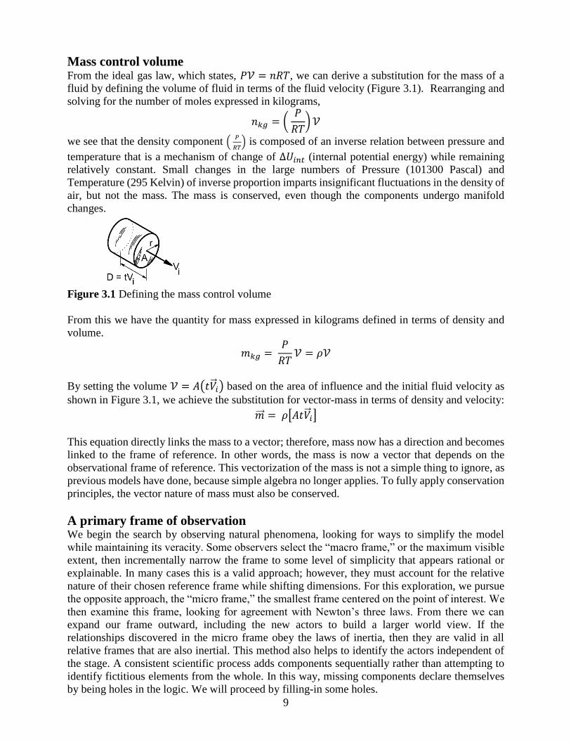
Mass control volume

From the ideal gas law, which states, 𝑃𝒱 = 𝑛𝑅𝑇, we can derive a substitution for the mass of a

fluid by defining the volume of fluid in terms of the fluid velocity (Figure 3.1). Rearranging and

solving for the number of moles expressed in kilograms,

𝑛𝑘𝑔 = ( 𝑃

𝑅𝑇) 𝒱

we see that the density component ( 𝑃

𝑅𝑇) is composed of an inverse relation between pressure and

temperature that is a mechanism of change of ∆𝑈𝑖𝑛𝑡 (internal potential energy) while remaining

relatively constant. Small changes in the large numbers of Pressure (101300 Pascal) and

Temperature (295 Kelvin) of inverse proportion imparts insignificant fluctuations in the density of

air, but not the mass. The mass is conserved, even though the components undergo manifold

changes.

Figure 3.1 Defining the mass control volume

From this we have the quantity for mass expressed in kilograms defined in terms of density and

volume.

𝑚𝑘𝑔 = 𝑃

𝑅𝑇𝒱 = 𝜌𝒱

By setting the volume 𝒱 = 𝐴(𝑡��𝑖) based on the area of influence and the initial fluid velocity as

shown in Figure 3.1, we achieve the substitution for vector-mass in terms of density and velocity:

�� = 𝜌[𝐴𝑡��𝑖]

This equation directly links the mass to a vector; therefore, mass now has a direction and becomes

linked to the frame of reference. In other words, the mass is now a vector that depends on the

observational frame of reference. This vectorization of the mass is not a simple thing to ignore, as

previous models have done, because simple algebra no longer applies. To fully apply conservation

principles, the vector nature of mass must also be conserved.

A primary frame of observation We begin the search by observing natural phenomena, looking for ways to simplify the model

while maintaining its veracity. Some observers select the “macro frame,” or the maximum visible

extent, then incrementally narrow the frame to some level of simplicity that appears rational or

explainable. In many cases this is a valid approach; however, they must account for the relative

nature of their chosen reference frame while shifting dimensions. For this exploration, we pursue

the opposite approach, the “micro frame,” the smallest frame centered on the point of interest. We

then examine this frame, looking for agreement with Newton’s three laws. From there we can

expand our frame outward, including the new actors to build a larger world view. If the

relationships discovered in the micro frame obey the laws of inertia, then they are valid in all

relative frames that are also inertial. This method also helps to identify the actors independent of

the stage. A consistent scientific process adds components sequentially rather than attempting to

identify fictitious elements from the whole. In this way, missing components declare themselves

by being holes in the logic. We will proceed by filling-in some holes.

10

The micro frame If we set our frame of observation to a point inside the forward opening of a Pitot static tube (Figure

3.2), we limit our world to that of the space inside the tube walls. One end is bounded by a liquid,

the other is bounded by an imaginary surface with area 𝐴′.

Figure 3.2 Inside the static tube

Inside this environment we could inflate a balloon at some point in time, then at some latter time

we find the balloon has changed size, but why? Because the pressure changed. What caused this

change? From this frame of reference, it is an unknown or imaginary force, because we have no

information beyond our frame boundaries. This first frame is non-inertial because of fictitious

forces; however, it shows where to look for the missing information.

If we increase our observational frame to include the immediate surroundings (Figure 3.3), we find

new elements that begin to build a stable model. We now include the wind with an initial velocity

of 𝑉𝑖 and a final velocity 𝑉𝑓

. The surface 𝐴′ is an imaginary boundary upon which the sum of the

forces equal zero, thus we have equilibrium according to Newton’s first law.

Figure 3.3 Fluid surface interaction on the area of impact

Relying on the fundamentals of Pitot’s pressure, we know the pressure inside the tube is caused

by the fluid impact that is proportional to the fluid density and the velocity-squared. We also know

the velocity inside the tube is zero, thus the velocity just outside surface 𝐴′ is also zero – this is the

velocity of stagnation 𝑉𝑠 = 0. Repeated experiments show the opening diameter of the Pitot static

tube to have no consequence other than to change the rate of response. Therefore, the force of

stagnation is constant over any surface with area 𝐴′. This frame has qualitative value because it

shows the fluid-surface interaction from which we may establish fundamental concepts.

11

Stagnation flow stream Here we reintroduce the control volume that is of the same area as 𝐴′ projected forward. This

concept is necessary for understanding the model’s structure and dynamics. As the wind

approaches the surface 𝐴′ it creates a pressure gradient, which ranges from stagnation pressure at

surface 𝐴′ to the ambient pressure at a reasonable distance. Because we know the wind continues

to move and we know the mass is conserved, we conclude the cause of the pressure to be of a

smaller control area, the area of stagnation 𝐴𝑠. If the area 𝐴′ of the control volume is defined by

the radius 𝑟′, then as 𝑟′ is reduced it reaches 𝑟𝑠, which defines the stagnation flow-stream area 𝐴𝑠.

This ‘stagnation volume’ is solely responsible for the kinetic force of stagnation; however, the

consecutive flow-streams must be assisting by providing lateral compression to the stagnation

flow-stream (Figure 3.4). The flow-stream could not exist in equilibrium without the surrounding

mass holding it stable, through the action of the pressure gradient.

Figure 3.4 Stagnation flow

The collision of stagnation is non-conservative because the air mass is losing internal potential

energy ∆𝑈𝑖𝑛𝑡 as the stagnation flow-stream reaches zero velocity. This stagnate mass must be

pushed aside, against the surrounding flow channels, to allow the next unit of mass to enter the

range of physical interaction, and this is a continuous process of change. When this system

reaches equilibrium, the rates of change become constant values, the sum of the forces are zero,

and the full control mass must be contributing to the overall change. Therefore, generalizing the

mass of stagnation from 𝐴′ to 𝐴𝑠 then to 𝐴 = 𝐴′ = 𝐴𝑠 is a reasonable assumption if the

observational frame is correctly identified as a closed system.

It is the lack of conservation in an inelastic collision that allows stagnation pressure to exist. The

vector-mass contained in the initial control volume undergoes a change of internal potential

energy ∆𝑈𝑖𝑛𝑡 as the collision occurs. For example, particle ‘front’ hits the surface and comes to

rest, while at time ∆𝑡/2 the particle ‘last’ is still traveling at the initial velocity. This change in

relative position requires work to be expended on the system of interaction during the collision.

After the collision, turbulent flow eddies mix the surrounding flow-streams, thus rebalancing the

pressure gradient downstream.

The wind must do work on itself to do work on the impinging surface, thus expending kinetic

energy to create the pressure gradient that establishes the stagnation pressure. This kinetic energy

loss cannot be accounted for by averaging arbitrary values before and after the plane of

interaction.

12

The static reference frame

To create our model, we use our imaginary surface with area 𝐴 as our point of reference (Figure

3.5). The wind is blowing from left to right, the positive 𝑥 direction. This wind has an initial

velocity ��𝑖 and must have some final velocity ��𝑓 that is an unknown variable. On the left we have

Force ‘a’ the force of the wind, on the right we have Force ‘b’ the force of Pitot’s pressure. On this

surface, the sum of the forces is always equal to zero, one side is kinetic stagnation, the other

Pitot’s pressure. This holds true for all reference frames.

Figure 3.5 Free body model

To establish meaningful values, this observational reference frame must include a scale of values

with a point of origin (Figure 3.6). All forces are parallel by nature and the vertical axis is

irrelevant. Thus, we can use the plane of interaction as the point of origin with a scale in units of

velocity given by the initial wind velocity ��𝑖. In this frame, populating the scene with actors now

becomes a sequential process of selecting fundamental equations and applying proper notation.

Figure 3.6 The static reference frame

13

Building the static equations

The stagnation pressure as measured by the Pitot static tube is:

�� =1

2𝜌𝑉𝑖

2

This pressure on a surface of area 𝐴 is a force, therefore:

�� =1

2𝜌𝐴𝑉𝑖

2

This force exerted during a time interval ∆𝑡 is impulse, resulting in the key that fits momentum’s

lock.

𝐽 =1

2𝜌𝐴𝑡𝑉𝑖

2

Kinetic energy was discussed previously in relation to the stagnation flow stream. We have already

generalized the area. However, the final velocity is that of stagnation or zero, and keeping it in the

equations is helpful while applying vector analysis. The equation for the change of kinetic energy

of wind in a static reference frame is given by the following equation. This is a non-conservative

quantity.

∆𝐾 = 1

2𝜌[𝐴𝑡��𝑖] (��𝑠

2− 𝑉𝑖

2

)

Momentum is the controlling function because it must be conserved. The total control mass

𝜌[𝐴𝑡��𝑖] will change momentum by losing velocity during impact. The change of momentum is

therefore linked to the final velocity of the wind. Until now, this final velocity has been predefined

by assumption. The change in momentum of the wind is given by:

Δ�� = 𝜌[𝐴𝑡𝑉𝑖](��𝑓 − 𝑉𝑖

)

Applying Newton’s third law of force bonding −��𝑎 = ��𝑏 to the second law Δ�� = 𝐽 identifies the

direction the key fits the lock. If force ‘b’ is equal to the opposite of force ‘a’ and force ‘a’ is Δ��,

then we want the opposite, or −Δ��. This would result in the proper momentum equation:

−Δ�� = −𝜌[𝐴𝑡𝑉𝑖](��𝑓 − 𝑉𝑖

)

If we factor the negative sign into the right side velocity function, we get a neater equation that

helps remove confusion. First it removes the pesky negative sign, insuring it doesn’t get lost.

Second, ��𝐹 will always be less then ��𝑖 thus Δ�� is a negative number. −Δ�� is a positive number,

therefore this form represents the equation in terms of positive numbers. This also helps orient the

vector substitutions for visual comparison. This switch will be used regularly throughout the

remaining text, so watch your opposites.

−Δ�� = 𝜌[𝐴𝑡𝑉𝑖](𝑉𝑖

− ��𝑓)

Applying the same reasoning to the equation for kinetic energy we get the following form:

−∆𝐾 = 1

2𝜌[𝐴𝑡��𝑖] (��𝑖

2− 𝑉𝑠

2

)

14

Applying Pitot’s static impulse to Newton’s Second Law

We can now neatly unlock Newton’s second law, resulting in a balanced equation founded in the

certainty of Pitot’s value for stagnation pressure. By combining equations, we achieve the

fundamental form of Pitot’s law in action.

𝜌[𝐴𝑡𝑉𝑖](𝑉𝑖

− 𝑉𝑓 ) =

1

2𝜌𝐴𝑡𝑉𝑖

2

We now have one equation with only one unknown ��𝑓, and if we solve for ��𝑓 it looks like this:

𝜌[𝐴𝑡𝑉𝑖](𝑉𝑖

− 𝑉𝑓 ) =

1

2𝜌𝐴𝑡𝑉𝑖

2

𝑉𝑖(𝑉𝑖

− 𝑉𝑓 ) =

1

2𝑉𝑖

2

(𝑉𝑖 − 𝑉𝑓

) =1

2��𝑖

𝑉𝑓 = 𝑉𝑖

−1

2𝑉𝑖

𝑉𝑓 =

1

2𝑉𝑖

This is a significant result, because we now know a true, natural value for the final velocity that

has been the point of intense debate. The Betz model used a convoluted balancing act to rationalize

his thesis.

No power here! This is a static observational reference frame, the surface 𝐴 represents a bounding force that

negates the force of kinetic impact converting energy to heat and turbulent flow vortices along

with the initial change of internal potential energy. There is no external work being done to the

system or by the system – there is no power in this reference frame. There is no displacement of

the surface during the application of force (force multiplied by displacement) [ ��∆𝑑 ], therefore

the force has done no work.

Mathematically, the power can be found in kinetic energy; however, this would be physically

incorrect. The necessary actors for this part are not yet present, however the missing dialog is now

reasonable to express as potential power in a static frame of reference, like this:

𝑃𝑜𝑤𝑒𝑟 = 1

2𝜌𝐴��𝑖 (��𝑖

2− 𝑉𝑠

2

)

𝑃 = 1

2𝜌𝐴��𝑖 (��𝑖

2)

𝑃𝑠𝑡𝑎𝑡𝑖𝑐 = 1

2𝜌𝐴��𝑖

3

This equation is familiar. Unfortunately, it is incorrect to imply any meaningful dialog based on

supposition that the actor exists. This result is only a marker indicating the need for further

expansion of our observational frame of reference.

15

4. Expanding to Dynamic Reference Frames

By shifting or transforming our point of reference to a point relative to both the wind and the

surface, we enter a dynamic frame of reference, Figure 4.1, by placing reference frame u in motion

relative to the earth frame. This represents the macro frame in which we wish to know the solution

for extractable power. The observational reference frame of the Earth is the common frame of

reference used in most studies to date. The new model looks similar to Figure 1.2 in that it has

three vectors, but we already asserted this to be incorrect. Now, we will discover why it is

insufficient.

The macro reference frame If all motion is relative and if the Pitot tube is also in relative motion, then the Pitot tube would

still be measuring the stagnation pressure relative to its own motion. If the Pitot tube’s surface area

𝐴′ was also the surface of a wind turbine, then it would also be measuring instantaneous force on

the turbine surface during a continuous time interval, and by extension, power.

Figure 4.1 The macro reference frame

Reference frame “u” is that of a surface with area 𝐴, which is that of the Pitot tube, and this surface

may be in motion relative to frame “e” (Figure 4.1). The x axis is in units of velocity given by ��𝑖

and the new vector, ��𝑢 is the vector representing the velocity of surface “u”. The question is, are

the valid equations in frame “u” also valid in frame “e”? We know that all motion is relative, which

instructs us to evaluate the motions of our system that identify the vector chain of relative linkages.

If the chains close, we have a bridge between reference frames. Algebraically, this is done using

vector addition with relative notation [7].

16

Identifying the relative vectors In Figure 4.2, we have the correct number of vectors representing the linkages of relative motions

between each object with proper subscript notation, resulting in the following list of vectors:

Initial wind velocity relative to the earth ��𝑖|𝑒

Final wind velocity relative to the earth ��𝑓|𝑒

Velocity of object “u” relative to the earth ��𝑢|𝑒

Initial wind velocity relative to object “u” ��𝑖|𝑢

Final wind velocity relative to object “u” ��𝑓|𝑢

Figure 4.2 Relative vectors

The vector bridge Linking this chain of vectors into a full bridge between the static frame u and the dynamic frame

e is necessary for completing the final equations because of the inherent directional nature of

relative vector addition. This chain links the initial wind velocity through the converter to the final

wind velocity in terms relative to the earth frame.

The original vector ��𝑖 became the vector ��𝑖|𝑢 Therefore, ��𝑖|𝑢 = ��𝑖|𝑒 − ��𝑢|𝑒 becoming a link

between the wind, the earth, and object “u”.

The original vector ��𝑓 became the vector ��𝑓|𝑢. Our earlier result provides that ��𝑓 =1

2��𝑖, therefore

becoming ��𝑓|𝑢 =1

2��𝑖|𝑢.

The new vector ��𝑢|𝑒 is defined as being some portion of the wind speed ranging from 0 to 1.

Therefore, we have the term ��𝑢|𝑒 = 𝑥��𝑖|𝑒 for x between 0 and 1.

The new vector ��𝑓|𝑒 has the relationship ��𝑓|𝑒 = ��𝑓|𝑢 + ��𝑢|𝑒.

Finally, we have the original wind velocity relative to the earth ��𝑖|𝑒 that is our constant input value.

17

In summary, we have the vector relations as follows:

��𝑖|𝑒 = 𝑐𝑜𝑛𝑠𝑡𝑎𝑛𝑡

��𝑓|𝑒 = ��𝑓|𝑢 + ��𝑢|𝑒

��𝑢|𝑒 = 𝑥��𝑖|𝑒

��𝑖|𝑢 = ��𝑖|𝑒 − ��𝑢|𝑒

��𝑓|𝑢 =1

2��𝑖|𝑢

These relative equations provide a link between any two objects, thus creating a bridge between

the two reference frames. If all links close, we have a bridge. Without the final velocity 𝑉𝑓|𝑢 these

links do not close.

First dynamic reference frame Figure 4.3 shows a complete frame of reference in which we have the necessary components to

answer our question and close the links. The vector bridge is shown graphically to the right of the

static frame. This box contains the vector equations that link the inner and outer vectors, thus

bridging the frames. The remaining vector relations are needed to reduce the equations in terms of

the initial wind velocity ��𝑖|𝑒.

Figure 4.3 Macro frame with vector bridge.

So let’s reexamine the valid equations from frame “u” by updating the notations. The stagnation

pressure relative to “u” as measured by the Pitot static tube is

�� =1

2𝜌��𝑖|𝑢

2

18

This pressure on a surface of area 𝐴 is a force that is relative to “u”, therefore:

�� =1

2𝜌𝐴��𝑖|𝑢

2

This force exerted during a time interval ∆𝑡 is the impulse 𝐽 relative to “u”,

𝐽 =1

2𝜌𝐴𝑡��𝑖|𝑢

2

The kinetic energy then is represented by the following equation. It should be noted here that the

mass component does not change as expected [as from “i” to “i|u”] because the vector-mass is

related to the initial control volume in both frames, therefore “i” becomes “i|e” where the change

in velocity is relative to the object “u”.

−∆𝐾 = 1

2𝜌[𝐴𝑡��𝑖|𝑒] (��𝑖|𝑢

2− ��𝑠

2)

The potential static power then becomes

𝑃 = 1

2𝜌[𝐴��𝑖|𝑒] (��𝑖|𝑢

2− ��𝑠

2)

The momentum is given by the following equation without special note:

−Δ�� = 𝜌[𝐴𝑡𝑉𝑖|𝑢 ](��𝑖|𝑢 − ��𝑓|𝑢)

Plotting these equations results in an unremarkable graph reflecting the nature of the functions that

behave as expected (Figure 4.4). One point of reference, however, did stand out as a clue to

investigate further. At the initial wind speed of ��𝑖|𝑒 = 1, all equations have the same value.

Figure 4.4 Plot of static equations

19

Same riddle, new perspective These equations hold true in the static frame; however, they do not reflect dynamic motion

correctly. We expanded our frame of reference but we did not change perspective. We left the 𝑥

axis as velocity given by ��𝑖|𝑒 for all positive values of x.

However, if we change the axis value to the velocity of object “u” and ��𝑢|𝑒 = 𝑥��𝑖|𝑒 our reference

frame is now dynamic and relative to object “u” (Figure 4.5).

Figure 4.5 The dynamic reference frame

This is a ‘Galilean transform’ in one dimension. What happened? In the static frame u the 𝑥 axis

is ��𝑖|𝑒, and we transformed our observational frame of reference along with our perspective by

changing from the wind speed being our plot axis to the velocity of object “u” ��𝑢|𝑒, in the earth

frame. In the static frame, only the wind was moving from left to right – with no reference to the

larger picture. We then moved to the first dynamic frame where the wind and surface were moving

to the right at different velocities while our perspective was not moving. In this final frame, the

observer is now traveling to the right at the same rate as object “u” or ��𝑢|𝑒. In other words, the

earth is now moving to the left relative to frame “u” and the wind is moving to the right. The

transform from ��𝑖|𝑒 to ��𝑢|𝑒 is found in the relation ��𝑢|𝑒 = 𝑥��𝑖|𝑒. The change of axis values is

achieved by multiplying the axis value by 𝑥, thus if we apply this to all equations they pass from

the static “micro” frame into the dynamic “macro” frame, producing valid equations in both frames

of reference.

20

The dynamic equations Now let’s reexamine the valid equations from static frame “u” by applying the transformation to

our static equations. The dynamic stagnation pressure relative to “u” as measured by the Pitot static

tube is

�� =1

2𝜌𝑥��𝑖|𝑢

2

This dynamic pressure on a surface of area 𝐴 is a dynamic force that is relative to “u”, therefore:

�� =1

2𝜌𝐴𝑥��𝑖|𝑢

2

The dynamic force exerted during a time interval ∆𝑡 is the dynamic impulse relative to “u”,

𝐽 =1

2𝜌𝐴𝑡𝑥��𝑖|𝑢

2

The dynamic kinetic energy is then represented by the following equation. It should be noted here

that the mass component now changes to 𝑥��𝑖|𝑒 that is also ��𝑖|𝑢. When the velocity of object “u” is

zero, then ��𝑖|𝑢 is ��𝑖|𝑒 because ��𝑖|𝑢 = ��𝑖|𝑒 − ��𝑢|𝑒. This equation implies that the vector-mass is now

relative to the object “u”, while the change in velocity again remains relative to the object “u”:

−∆𝐾 = 1

2𝜌[𝐴𝑡𝑥��𝑖|𝑒] (��𝑖|𝑢

2− ��𝑠

2)

The potential static power becomes a real quantity by transformation into a dynamic model. We

now have the equation for Power relative to the earth frame – this is usable energy. Further, the

equation represents the change of external potential ∆𝑈𝑒𝑥𝑡 in the static reference frame that helps

balances the work energy equation of that frame.

𝑃 = 1

2𝜌[𝐴𝑥��𝑖|𝑒] (��𝑖|𝑢

2− ��𝑠

2)

The following equation represents the dynamic momentum, an unexpected result because as we

build the equation we find, through graphical vector analysis, that the change in velocity is now

that of the earth frame of reference: ��𝑖|𝑢 changed to ��𝑖|𝑒. Where the momentum velocity change

was previously relative to the static frame “u”, now it is transformed to be relative to the dynamic

frame “e”.

−Δ�� = 𝜌[𝐴𝑡𝑥��𝑖|𝑢](��𝑖|𝑒 − ��𝑓|𝑒)

21

Applying Pitot’s dynamic impulse to Newton’s Second Law

We can now apply the same solution as in the static frame to Newton’s impulse-momentum

equations in the dynamic frame:

𝜌[𝐴𝑡𝑥��𝑖|𝑢](��𝑖|𝑒 − ��𝑓|𝑒) =1

2𝜌𝐴𝑡𝑥��𝑖|𝑢

2

��𝑖|𝑢(��𝑖|𝑒 − ��𝑓|𝑒) =1

2��𝑖|𝑢

2

��𝑖|𝑒 − ��𝑓|𝑒 =1

2��𝑖|𝑢

��𝑓|𝑒 = ��𝑖|𝑒 −1

2��𝑖|𝑢

Without resolving the relative vectors, this would be our final step, so we need to frame the result

in terms of the original wind velocity ��𝑖|𝑒. We know that ��𝑖|𝑢 = ��𝑖|𝑒 − ��𝑢|𝑒 and that ��𝑢|𝑒 = 𝑥��𝑖|𝑒.

Combining equations, we get the following value for ��𝑖|𝑢

��𝑖|𝑢 = ��𝑖|𝑒 − 𝑥��𝑖|𝑒

��𝑖|𝑢 = ��𝑖|𝑒(1 − 𝑥)

Substituting this value back into our equation, we get the following solution:

��𝑓|𝑒 = ��𝑖|𝑒 −1

2��𝑖|𝑒(1 − 𝑥)

The solution resolves to the following equation for the final velocity relative to the earth:

��𝑓|𝑒 =1

2��𝑖|𝑒(1 + 𝑥) [𝑎]

When we transform ��𝑓|𝑢 =1

2��𝑖|𝑢 from the static frame into the dynamic frame, we have

𝑥��𝑓|𝑢 =1

2𝑥��𝑖|𝑒(1 − 𝑥)

We also have the bridging relationship of ��𝑓|𝑢 = ��𝑓|𝑒 − ��𝑢|𝑒 that results in the following solution:

𝑥(��𝑓|𝑒 − 𝑥��𝑖|𝑒) =1

2𝑥��𝑖|𝑒(1 − 𝑥)

𝑥��𝑓|𝑒 − 𝑥2��𝑖|𝑒 =1

2𝑥��𝑖|𝑒 − 𝑥2��𝑖|𝑒

𝑥��𝑓|𝑒 =1

2𝑥��𝑖|𝑒 − 𝑥2��𝑖|𝑒 + 𝑥2��𝑖|𝑒

𝑥��𝑓|𝑒 =1

2𝑥��𝑖|𝑒(1 − 𝑥 + 2𝑥)

��𝑓|𝑒 =1

2��𝑖|𝑒(1 + 𝑥) [𝑏]

This solution [b] confirms the previous results [a]. We also have the vector solution for ��𝑓|𝑒 as

��𝑓|𝑒 = ��𝑓|𝑢 + ��𝑢|𝑒. Therefore, we have three independent solutions that resolve to the same

function.

22

Pitot’s power

So far we have derived power from the change in kinetic energy; this is a valid solution and our

equations are in the proper form. However, how could we check or confirm this result, considering

that kinetic energy is non-conservative?

By returning to the fundamental concepts, we know that 𝑃 = ��∥��. We also now have the necessary

components to directly solve for Power because �� is the velocity of the object being acted upon,

�� = ��𝑢|𝑒.

𝑃 = ��∥��𝑢|𝑒

Selecting the correct force is necessary because of the relative reference frames; graphical analysis

was used to verify that the force is relative to the surface in the static frame. Substitution then

yields:

𝑃 = 1

2𝜌𝐴(��𝑖|𝑢)

2 ��𝑢|𝑒 [𝑐]

This form of the equation expresses the relative nature of the vectors and will be seen again. Setting

this in terms of the initial wind speed ��𝑖|𝑒 gives us the following:

𝑃 = 1

2𝜌𝐴(��𝑖|𝑒 − 𝑥��𝑖|𝑒)

2 𝑥��𝑖|𝑒

By rearranging and simplifying we have

𝑃 = 1

2𝜌𝐴��𝑖|𝑒

3𝑥(1 − 𝑥)2

If we then say that 𝑥(1 − 𝑥)2 is the ‘coefficient of power’ 𝜄 ,we can examine its behavior

separately, thus allowing us to derive the following equation for power:

𝑃 = 𝜄 1

2𝜌𝐴��𝑖|𝑒

3 [𝑑]

Before we examine 𝜄, let’s review the power derived from kinetic energy.

𝑃 = 1

2𝜌[𝐴𝑥��𝑖|𝑒] (��𝑖|𝑢

2− ��𝑠

2)

If we rearrange and simplify, we get

𝑃 = 1

2𝜌𝐴(��𝑖|𝑢)

2 ��𝑢|𝑒

This is the same equation that we found in equation [c] by substitution into 𝑃 = ��∥𝑣. Therefore, if

we again put this in terms of ��𝑖|𝑒 we get Pitot’s power equation:

𝑃 = 𝜄 1

2𝜌𝐴��𝑖|𝑒

3 [𝑒]

Equations [d] and [e] are the same quantity, approached from both sides of Newton’s cradle. Power

derived from kinetic energy fully agrees with power derived from impulse, harmoniously

conserving nature’s laws.

23

Pitot’s power coefficient

The new coefficient �� represents the absolute maximum power coefficient of any power extraction

device in a free-flowing fluid environment.

In review, the stagnation pressure on a nonporous surface with zero velocity is the maximum force

the wind will exert on that surface. The maximum force is then relative to the surfaces velocity

��𝑢|𝑒, diminishing as this velocity increases from 0 to 1. The Pitot static tube measures the

stagnation pressure and is accurate during relative motion. Therefore, 𝜄 must be derived from

Pitot’s power equation, rather than from the Betz distorted geometric probabilities and drag

coefficients.

Optimum power ratio

Many previous windy theories evaluated the velocity component of momentum by simply

concluding an optimum ratio based on some convoluted rational. The following provides an

optimum ratio from a different perspective – abridged graphical analysis.

Figure 4.6 the natural power function of fluids

Plotting �� = 𝑥(1 − 𝑥)2 results in a graph that reflects the natural power function of fluids, this is

a perfect power curve (Figure 4.6). One point of reference is of great interest, that of the maximum

value: this occurs when 𝑥 =1

3 . Solving our equation at maximum value, we find

𝜄 =1

3(1 −

1

3)

2

𝜄 =1

3(

2

3)

2

𝑀𝑎𝑥𝑎𝑚𝑢𝑚 �� =4

27

Placing this value back into Pitot’s power equation results in the absolute maximum extractable

power of any device in a free flowing fluid environment.

𝑃 = 2

27𝜌𝐴��𝑖|𝑒

3

This is a significant result in many regards: note especially that 𝜄 =4

27, which is the same

maximum value predicted in the current drag model, then declared inferior to lift. Even though the

Betz model used faulty assumptions, the results of his optimum momentum ratio is correct.

24

This analysis is also based on the optimum momentum ratio from a known value of a “drag model”,

better known as an “impulse turbine”. Therefore, the impulse turbine defines maximum power

extraction contrary to popular beliefs.

What about efficiency?

The Betz limit states that we can only extract 59.3 percent of the total power contained in an air

mass. similar proportionalities are also found in parallel studies of thermodynamic cycles [8] and

endoreversible collisions [9]. The Carnot cycle is a theoretically perfect model, while the Novikov

cycle accounts for the ∆𝑈𝑖𝑛𝑡 as the flow enters the system. Our situation is similar, in that Betz is

a theoretical model without real values – but we can now define the value of ∆𝑈𝑖𝑛𝑡 using real

numbers, providing a real value for the proper completion of the original work-energy equation.

Solving the lost energy question By reversing the logic (i.e., start with the new result, then reevaluate the environmental conditions

necessary to unify the fundamental equations), it goes like this: If maximum extractable power is 2

27𝜌𝐴��𝑖

3 and is 59.3 percent of the maximum potential power, then

2

27÷

1

8=

16

27= . 593 or 59.3

percent; thus; the maximum potential power of fluids is 1

8𝜌𝐴��𝑖

3. Then, if

1

8𝜌𝐴��𝑖

3 is maximum

potential power and the perfect kinetic collision is 1

2𝜌𝐴��𝑖

3, then (∆𝑈𝑖𝑛𝑡) must be

3

8𝜌𝐴��𝑖

3. This

leads back to the broadly significant conclusion that the Pitot power curve is the ultimate

extractable power of fluids.

The power coefficient of 16

27 was cited by Betz as being the superior lift-based coefficient.

Ironically, by using the incorrect value for maximum potential he achieved the correct ratio with

inflated significance. Both systems have the exact same maximum potential – until we understand

that lift is wasting potential through excessive tip speeds.

Pitot’s efficiency is therefore the real limit. 𝜂 =2

27𝜌𝐴��𝑖

3

1

8𝜌𝐴��𝑖

3 =16

27= . 593

25

5. The New Model of Fluidic Power Extraction

Diagram 5.1 is a model of fluid interaction and power extraction based on the Novikov diagram,

which puts the values and interactions in context [10]. From left to right: the original control volume

with velocity ��𝑖|𝑒 and a quantity of energy 𝑈𝑖 enters the zone of impact. At this point the fluid has

a theoretically perfect potential power of 1

2𝜌𝐴��3. In the zone of impact, the fluid geometry

changes, while energy is expended in (∆𝑈𝑖𝑛𝑡). Quantities in this zone are beyond calculation

because the mass in this zone is experiencing a deceleration, therefore interactions are non-inertial.

In this model, the surface plane of interaction is the perfect converter, being a simple, nonporous

surface – that of the Pitot static tube where the internal potential (𝑈𝑖𝑛𝑡) now has a maximum of 1

8𝜌𝐴��3. Here we have the Pitot engine composed of reference frames “u” and “e”. The Pitot

engine perfectly defines the momentum and energy further, resulting in the maximum extractable

power ∆𝑈𝐸𝑥𝑡 of 2

27𝜌𝐴��𝑖

3. Continuing to the right we have the final energy 𝑈𝑓 that can now be

expressed as 11

216𝜌𝐴��𝑖

3 and the final wind velocity ��𝑓|𝑒 that were both defined in Pitot’s engine.

We can assert these final values as the results of interaction however we now have turbulent

conditions where any further analysis is meaningless.

Figure 5.1 A model of fluid interaction and power extraction

This model represents a larger reference frame that provides a holistic understanding of the

system’s interactions. Our analytical reference frame “e”, while complete, did not contain

information about the mechanism of collision. To answer the question of Power derived from the

work energy equations, we need to accumulate all forms of energy conversions. In the proper form,

the comprehensive equation requires knowledge of the manifold changes experienced by the fluid

during collision:

∆𝑊 = ∆𝐾 + ∆𝑈𝑖𝑛𝑡 + ∆𝑈𝑒𝑥𝑡 + ∆𝒰𝑜𝑡ℎ𝑒𝑟

From the information gained by deriving Pitot’s power, we can develop reasonable conclusions as

to environmental values, including (∆𝑈𝑖𝑛𝑡), because we have the value for maximum extricable

power ∆𝑈𝑒𝑥𝑡 and the change of kinetic energy.

26

6. Intense Graphical Analysis

The completed frame Figure 6.1 incorporates all the previous descriptions. Some conclusions are not apparent or

presentable in this format, but we can now clarify and highlight key points.

Figure 6.1 The completed frame of reference

The structure of these equations is deliberate in order to emphasize that the mass 𝜌[𝐴𝑡��𝑟] is a

separate component that has a vector relation to its position and function in the equation. The mass

changes nature relative to its reference frame and relative motion. The velocity component is a

balance between vectors, consistent in its frame of reference. Extending this method to other

systems requires resolving all vectors into the earth frame of reference while keeping the

perspective of the surface.

This model allows us to express the functions in terms of the initial wind velocity, providing the

solution for maximum extractable power as 2

27𝜌𝐴(��𝑖|𝑒)

3. However, the equation should be 𝑃 =

1

2𝜌𝐴��𝑢|𝑒(��𝑖|𝑢)

2 in order to insure proper vector selection.

Power is relative to the combined motions and must first satisfy 𝑃 = ��∥��. These are vectors! A

vector chain is the linking between all vectors such that any one may be described in terms of the

others. Vectors with relative motion can link into a chain, and if this chain is complete we have a

bridge. The chain in this model is only completed by applying Pitot’s impulse to the momentum

equation, otherwise any solution dissolves. Predefining the final velocity forces the system out of

balance even if the guess was partially correct, as in the Betz model. We know the impulse because

we now know how to measure it. From this known impulse we can solve the momentum equation

without supposition.

27

The kinetic energy exhibits characteristics found in the relative nature of the vector mass 𝜌[𝐴𝑡��𝑟].

The mass in the earth frame 𝜌[𝐴𝑡𝑥��𝑖|𝑢], by vector chain, is now relative to the velocity of surface

“u” as 𝜌[𝐴𝑡��𝑢|𝑒].

Momentum must be conserved; therefore, Pitot’s power is the gold standard to which the kinetic

energy must be balanced. Deriving power from kinetic energy is error prone because kinetic energy

is not conserved. Pitot’s power provides us a real value to balance the energy of perfect kinetic

interaction, with the maximum potential of a fluid. One is solid and perfectly conserved, the other

is fluidic, non-conservative, and irreversible.

Plotting equations Using Figure 6.1 as our model of a perfect fluidic power conversion, we can check the data by

plotting the equations. During the graphical analysis, Pitot’s power coefficient was used as the

ideal curve. By iteratively testing all vector permutations of the fundamental equations we can

visually confirm the validity of the vector relationships and position in the equations. This is

plotted in the Earth's reference frame from the perspective of the surface. In Figure 4.1 it was noted

that all equations have the same value if initial velocity was equal to one, ��𝑖|𝑒 = 1. Thus, by

converting all the vectors into unit vectors and setting all remaining variables to the value of one,

we achieve a unit vector plot allowing the comparison of equations with the perfect curve. All

valid equations have been plotted and grouped by reference frame (Figure 6.2).

Figure 6.2 A unit vector plot comparing equations with the perfect power curve

The equations from frame “u” start at maximum value when the surface has zero velocity, the

“static” state. As surface “u” begins to move, the forces decrease until the velocity of “u” reaches

the original wind speed, whereupon there is no relative motion. This set also includes the kinetic

power probability equation. The equations from frame “e” perfectly match Pitot’s power

28

coefficient. There is no power if surface “u” is not moving; however, the static forces are

maximum. As surface “u” begins to move, power is generated – reaching a maximum output when

surface “u” reaches one third the wind velocity, then begins to drop as the relative static forces

diminish. The balance between force and velocity is given by the principal equation 𝑃 = ��∥��. As

force decreases, so does power. If velocity �� equals zero, we have no power. As �� increases, so

does power. In our case, force is decreasing as velocity increases, reaching an optimum ratio when

velocity ��𝑢|𝑒 equals one third the initial wind velocity. As the force approaches zero, so does the

power.

The three maximum power formulas perfectly represent the relation of energy states. Power is the

rate that work is done. Work is a change in energy. These formulas provide a natural solution to

the internal energy change, shown as maximum theoretical kinetic energy in an elastic collision at

the top to the maximum potential of a fluid in relative motion based on the known value of Pitot’s

power.

Plotting vectors Plotting the vectors in the same coordinate system shows their relation to the surface “u” in unitary

terms, reflecting only the change in vector value (Figure 6.3).

Figure 6.3 A plot of the vectors showing their relation to the surface “u”

The initial wind speed ��𝑖|𝑒 is our input variable and is set to a constant value of 1 m/s. The velocity

of surface “u’ increases from 0 to the original wind velocity ��𝑖|𝑒. The initial wind velocity relative

to surface “u” ��𝑖|𝑢 decreases from 1 to 0 as ��𝑢|𝑒 increases from 0 to 1. The final velocity relative

to the earth frame ��𝑓|𝑒 increases from 1

2��𝑖|𝑒 to the velocity of the wind as the final velocity relative

to “u” decreases from 1

2��𝑖|𝑒 to zero.

From the perspective of graphical analysis, analytical geometry, and vector bridging, these are

very nice plots in their pure simplicity – they reflect the perfect model.

29

7. Vector Analysis of Lift Turbines

In Figure 7.1 we have a typical horizontal-axis wind turbine. By taking a cross-section of one of

the airfoil elements, we can establish an observational frame of reference in the micro respect.

Because it is attached to a rotational reference frame, this frame is non-inertial. However, in the

static sense we can analyze the vectors acting on this element. Now, by rotating our perspective to

be orthogonal with this frame, we can start to describe the interaction of forces.

Figure 7.1 Cross-section of a typical horizontal-axis wind turbine

Tip speed vectors Figure 7.2 represents our micro frame of reference with a rotational velocity of zero. The airfoil is

oriented such that the angle of attack is optimum for maximum lift. In this static condition, the

airfoil will experience its maximum lift potential at the given wind speed. Increasing the wind

speed will increase the lift. By looking at the vectors, we see that the lift in this configuration is

completely tangential. The drag and the resultant lift are constrained forces.

Figure 7.2 The micro frame of reference with the rotational velocity of zero

30

Figure 7.3 represents our micro frame of reference with the rotational velocity equal to the wind

speed. The resultant velocity is now ��𝑤√2 . The angle of attack is maintained to achieve maximum

lift. As the blade twist angle decreases, the lift vector is rotated to remain perpendicular to the

relative or resultant wind velocity. This rotation decreases the tangential lift vector, which

therefore decreases the force in the direction of motion. This rotation also creates an axial lift

component that becomes additive to the drag forces in the axial direction, causing a coning effect

on the airfoil as it tries to fly down wind.

Figure 7.3 The micro frame of reference with the rotational velocity equal to the wind speed

In Figure 7.4, we allow the rotational velocity to become greater than the initial wind velocity. The

current high output/low speed horizontal turbine has a tip speed ratio of 3:1 as depicted in this

diagram. Here we see the blade twist angle has been reduced even further. As the velocity of the

airfoil increases, the lift is rotated further to the downwind position, which again reduces the

tangential lift and increases the axial lift (see Figure 7.3). The energy lost by this rotation is the

energy that increases the airfoil rotational velocity and the axial lift. The energy contained in the

initial control volume at the initial velocity is converted to rotational velocity and extremely

counterproductive axial forces. At some point, the rotational velocity and wasted axial forces will

reach a balance with the original energy of the wind, whereupon no power may be extracted. As

the tangential lift approaches zero, so does the force in the power equation. The theoretical

rotational velocity may approach infinity; however, as the force in the direction of rotation

approaches zero, so does power. Therefore, rotational tip speed ratios greater than 1:1 are highly

inefficient.

Figure 7.4 The micro frame of reference with the rotational velocity greater than the wind speed

31

Figure 7.5 represents the vector changes from the three previous diagrams. As tip speed increases,

the tangential lift decreases, while at the same time the axial lift increases. Both of these conditions

reflect wasted potential. We must acknowledge that the lift vector was held unitary for descriptive

purposes. The lift force will increase dramatically as tip speed increases. The larger lift component

would result in a greater tangential lift that is also matched by a much greater axial lift component

as twist angle decreases.

Figure 7.5 Vector changes and tip speed

Shrouded turbines Shrouding or shielding creates a “bucket effect”. If we hold a bucket opening perpendicular to a

flow, it will have Pitot’s stagnation pressure, as shown in Figure 7.6(A). If we place a hole in the

bottom, we have the classic physics problem of applying Bernoulli’s theorem to our bucket as in

Figure 7.6(B). If this hole is smaller than the bucket opening, creating a funnel, the flow velocity

through will be reduced from its initial maximum velocity, thus restricting the maximum power to

the original bucket or shrouding surface. Because the wind will always go around rather than

through an obstacle, following the path of least resistance, shrouding does not increase energy-

extraction potential. Figure 7.6(C) shows the hole at the same size as the opening, and this

condition will still see less then maximum potential because the thin shrouding is still present and

is having an effect on the flow.

Figure 7.6 The bucket effect

Implications The energy contained in the control volume is proportional to the velocity of the wind relative to

the airfoil. If the original velocity of the wind is 2 m/s with a tangential velocity of 2 m/s than the

resultant velocity is 2.8 m/s; therefore, the maximum potential energy must be calculated using the

resultant velocity of 2.8 m/s. In effect, the horizontal turbine amplifies the original wind velocity

through tip speed, thus increasing the potential incoming energy – then converting the major

portion of this gain into wasted energy, not efficiency.

Only the force in the direction of rotation is power. The static force at the relative wind speed is

the maximum force this system can achieve because as rotation increases, the force in the direction

of rotation decreases, implying a balance between force and rotation. As the rotational velocity

increases, the tangential forces on the airfoil decrease at the same time the relative mass or resultant

energy has increased. The numerator has become smaller and the denominator has become larger.

32

The ability of this machine to amplify the wind creates a dynamic denominator in the efficiency

equation. Therefore, as tip speed increases, efficiency decreases exponentially.

𝜂 =��∥��

18 𝜌𝐴(��𝑅𝑒𝑙)

3

The maximum potential power of any system must be based on the relative velocity of the fluid

surface interface expressible in terms of the relative velocity.

𝑃𝑀 = 1

8𝜌𝐴(��𝑅𝑒𝑙)

3

By example By using data extracted from the Enercon corporation in Table 1, we can see the significance of

the requirement that the velocity relative to surface interaction be used in the maximum power

formula and the effect it has on HAWTs. The true efficiency calculation reflects the fact that as tip

speed increases above the original wind velocity, the energy is increasingly wasted in the axial lift

vector.

Table 1: Original data calculations

The moment of inertia in a rotating body is a point on the radius where the mass can be considered

as a point or ring mass. The tip speed does not represent the tangential velocity of the moment of

inertia for any system. A typical solution for the moment of inertia in this configuration is about

two thirds the original radius. Also adjusting the area A to a more appropriate number loosely

estimated to that of the surface area presented to the resultant wind velocity 𝑉𝑟, we see the original

efficiency becomes over-unity while the estimated efficiency approaches a truer representation of

reality (Table 2).

Table 2: Adjusted data calculations

Vw power 1/2ρAVi3 efficiency speed ω tip speed Vr 1/8ρAVr

3 True efficiency

m/s Watts Watts Cp RPM Radians m/s m/s Watts Cp

3 55,000 209,497 0.263 5 π/6 33.25 11.08 33.38 72,169,444 0.001

10 3,750,000 7,759,150 0.483 7 7π/30 46.55 4.65 47.61 209,337,998 0.018

16 7,580,000 31,781,478 0.239 9 3π/10 59.85 3.74 61.95 461,170,361 0.016

20 7,580,000 62,073,200 0.122 10 π/3 66.50 3.32 69.44 649,494,737 0.012

28 7,580,000 170,328,861 0.045 12 2π/5 79.80 2.85 84.57 1,173,133,672 0.006

Enercon E-126

new methodcalculated dataextracted data

Area = 12,668 m2 ( 136,357 ft

2 ) ρ = 1.225Radius = 63.5 m ( 208 ft )

tip speed

ratio

Vw power 1/2ρAVi3 efficiency speed ω tip speed Vr 1/8ρAVr

3 estimated

m/s Watts Watts Cp RPM Radians m/s m/s Watts Cp

3 55,000 34,911 1.575 5 π/6 22.17 7.39 22.37 3,617,452 0.015

10 3,750,000 1,292,988 2.900 7 7π/30 31.03 3.10 32.60 11,202,716 0.335

16 7,580,000 5,296,077 1.431 9 3π/10 39.90 2.49 42.99 25,676,802 0.295

20 7,580,000 10,343,900 0.733 10 π/3 44.33 2.22 48.63 37,183,935 0.204

28 7,580,000 28,383,662 0.267 12 2π/5 53.20 1.90 60.12 70,228,675 0.108

2/3 Radius = 42 m (137 ft)

tip speed

ratio

Enercon E-126

new methodcalculated dataextracted data

1/6 Area =2,111 m2

(22,722 ft2 ) ρ = 1.225

33

In Conclusion

Through a detailed analysis using fundamental physics without limiting assumptions combined

with a measurable quantity, we have redefined the Maximum Extractable Power of fluids. This

new model of Fluidic Power Extraction provides a holistic understanding of the perfect model

demonstrated through graphical analysis, wherein we have also demonstrated the true Maximum

Potential Power in a free-flowing environment.

We first redefined the mass control volume using the ideal gas law, showing the interrelation

between changing density and constant mass. We further establish that mass is a vector quantity

relative to a body’s motion. We provided a new perspective relative to the observational frames of

reference in which we clearly defined the static model in relation to a dynamic world view.

We then demonstrated that Pitot’s simple device and equation provide the key to Newton’s cradle

in which both momentum and kinetic energy must agree on the terms of collision. We show that

momentum controls the conservation function while kinetic energy is only that of the stagnation

flow stream and is a non-conservative quantity that is lost in the ∆𝑈𝑖𝑛𝑡 before the collision. Pitot’s

equation simply states, “Stagnation is the maximum pressure any system will experience.” From

this insight we concluded that Pressure is a Force and Force is an Impulse that naturally fits

Newton’s Second Law, the key discovery established in this presentation.

While providing an elaborate demonstration of reference frames, relative motion, and vector

analysis, we have demonstrated three solutions for ��𝑓|𝑒 that is the critically missing component of

previous studies that used simplified conditions on the final fluid velocity. We then achieved two

natural solutions for the Maximum Extractable Power: one from Impulse and one from Energy,

which together demonstrate perfect energy conservation.

The Power formula derived with Pitot’s equation is the maximum extractable power; therefore,

Pitot’s Power Coefficient 𝜄 = 𝑥(1 − 𝑥)2 defines the optimum power curve that also establishes

true Efficiency, the Maximum Power Potential and Limit.

Efficiency is a ratio of parts per total, but the total or maximum value used in previous studies

failed to account for internal losses, resulting in the ratio of 16/27 or 59.3 percent. Subsequent

studies of drag-style systems declared a ratio of 2/27 as being the maximum potential, in contrast

to the 16/27 of “superior” lift systems. The real question has always been, “59.3 percent of what?”

Our new model has established this maximum potential value, resulting in the same numerical

ratios at the true scale. In a roundabout way, our equation (2

27÷

1

8) =

16

27= . 593 = 59.3 percent

both destroys and confirms the Betz theorem. If he had started with a known value for the

maximum potential power, as we did, his formulation would have been in the correct proportional

scale. Thus, the drag method of analysis confirms our results of 2/27 that – combined with the true

maximum potential – reflects the same limit of 59.3 percent implied by Betz, but in the scale nature

intended.

The physics demonstrated here is based on the analysis of a new hybrid wind turbine design [11].

Equating the surface 𝐴 of an impulse turbine with that of a Pitot tube with surface area 𝐴′ means

we can measure the forces on that turbine surface. This study implies that a well-designed impulse

turbine could achieve the Pitot Limit of 59.3 percent.

34

We can therefore extrapolate significant conclusions from this study:

Drag is not a motivating force and cannot be fundamentally established for a random body.

Drag is the frictional force linked to aerodynamic lift. Using the friction of a system to

describe a body’s inertia only works if we have measured values from a static system of

known geometry, otherwise drag analyses remains theoretical to a random body.

The static forces represent maximum potential at the relative wind velocity.

Maximum Potential Power is relative to the velocity experienced at the point of conversion.

The Horizontal Axis Turbine amplifies the original wind velocity through tip speed, thus

increasing the potential incoming energy – then converts the major portion of this gain into

wasted energy, not efficiency.

By acknowledging that tangential lift is the only source of power for HAWTs, we can avoid

embarrassingly inflated claims.

The Vertical Axis Impulse Turbine has the same maximum potential as HAWTs of equal

area and relative wind velocity, as shown in the lost energy question.

Vector analysis has shown lift-based systems to be less efficient then a common “drag” or

Impulse Turbine, as demonstrated in Part 7.

The impulse turbine defines the Maximum Extractable Power, ∆��𝐸𝑥𝑡.

The impulse model defines the Efficiency and Limit of a free-flowing fluid.

The industry-wide biased attitude against Vertical Axis Impulse Turbines are based on faulty

assumptions and incomplete models, along with the oversimplification of Newton’s laws and

errors regarding conservation of energy, applied force, and power. By presenting my study into

the fundamental principles of wind power, I hope to change this myopic view and establish a valid

market for Vertical Impulse Turbines, spawning a revolution in innovation, design and application.

“HAWT’s are, in effect, Rube Goldberg perpetual motion machines operating above unity for the

sole purpose of converting money into wind. There is a better way.” … Don Harwood

35

References 1. Betz, A.: Windenergie und ihre Ausnutzung durch Windmühlen, Vandenhoek und

Rupprecht 1926; Viewg, Gøottingen, 1946.

2. Hartwanger, D., Horvat, A., 3D Modelling of a Wind Turbine Using CFD, NAFEMS

UK Conference 2008 "Engineering Simulation: Effective Use and Best Practice",

Cheltenham, UK, June 10–11, 2008, Proceedings.

3. Gorban, A.N., Gorlov, A.M., Silantyev, V.M.: Limits of the Turbine Efficiency for

Free Fluid Flow, Journal of Energy Resources Technology, December 2001, Volume

123, Issue 4, pp. 311-317.

4. Daniel Bernoulli, Hydrodynamica, 1738.

5. Hau, E.: Wind Turbines: Fundamentals, Technologies, Application, Economics, 2rd Ed.,

Springer Verlag 2006.

6. http://structurae.net/persons/henri-pitot 7. Arnold, V. I., Mathematical Methods of Classical Mechanics, 2rd Ed., Springer-Verlag,

1989.

8. Carnot, Sadi; Thurston, Henry (editor and translator), Reflections on the Motive Power

of Heat. New York: J. Wiley & Sons, 1890.

9. Novikov, I.I. The Efficiency of Atomic Power Stations. Journal Nuclear Energy II,

7:125–128, 1958. Translated from Atomnaya Energiya, 3 (1957), 409.

10. Wagner, K. A graphic based interface to Endoreversible Thermodynamics, TU

Chemnitz, Fakultät für Naturwissenschaften, Masterarbeit (in English).

11. Harwood, Don Aerostatic wing with slipstream turbine U.S. Patent pending

#29/499,923 and #14/463,856

Copyright © 2016 by Don Harwood. All rights reserved. No part of this publication may be

reproduced, stored in or introduced into a retrieval system, or transmitted, in any form, or by any

means (electronic, mechanical, photocopying, recording, or otherwise), without the prior

permission of the copyright holder. Requests for permission should be directed to Don Harwood,

CEO Aerostatic Enterprises.

36

𝑃 = 1

2𝜌𝐴��𝑢|𝑒(��𝑖|𝑢)

2

Aerostatic wing with slipstream turbine U.S. Patent pending #29/499,923 and #14/463,856