Wind Induced Pressure on ‘E’ Plan Shaped Tall Buildings

Jordan Journal of Civil Engineering, Volume 8, No. 2, 2014

- 120 - © 2014 JUST. All Rights Reserved.

Wind Induced Pressure on ‘E’ Plan Shaped Tall Buildings

Biswarup Bhattacharyya 1)

, Sujit K. Dalui 2)*

and Ashok K. Ahuja3)

1)

Post-Graduate Student, Department of Civil Engineering, Bengal Engineering and Science University,

Shibpur, Howrah, India. 2)

Assistant Professor, Department of Civil Engineering, Bengal Engineering and Science University,

Shibpur, Howrah, India. 3)

Professor, Department of Civil Engineering, Indian Institute of Technology Roorkee, Roorkee, India.

* Corresponding Author: Howrah-711103, West Bengal, India.

E-Mail: [email protected]

ABSTRACT

The present study demonstrates the pressure distribution on various faces of ‘E’ plan shaped tall buildings

under wind excitation. Experimental and analytical studies were carried out using wind angles varying from

0° to 180° with an interval of 30°. The experimental study was conducted by open circuit boundary layer

wind tunnel; whereas the analytical study was conducted with Computational Fluid Dynamics (CFD)

technique using ANSYS CFX software package using k-ε turbulence model. A rigid model (made of perspex

sheet) was used for wind tunnel test with a model scale of 1:300. Mean pressure coefficients of all the faces

are found for all wind incidence angles and pressure contours are plotted on all the surfaces for 0° wind

angles. Mean pressure coefficients are also calculated by CFD technique and the results have a good

agreement with experimental results. Also, pressure contours on all the faces for a 0° wind angle are plotted

and the contours are almost similar to those of experimental investigation. The flow pattern around the

building model is also shown to understand the variation of pressures on different faces for a particular wind

angle.

KEYWORDS: Tall building, Wind tunnel test, Mean pressure coefficient, Computational Fluid

Dynamics (CFD), Flow pattern.

INTRODUCTION

Wind engineering is best defined as the rational

treatment of interactions between wind in the

atmospheric boundary layer and man and his works on

the surface of Earth. In the context of urbanization,

land area is not expanding but population is increasing

daily especially in cities. So, the requirement of high

rise buildings is urgently needed. Such buildings may

be of conventional shape in plan or may be irregular.

Such irregular plan shape buildings are mostly efficient

to utilize total land area. Wind load is mostly critical in

case of high rise buildings. Pressure variation and force

coefficient for such conventional plan shape buildings

(i.e., rectangular, square… etc.) are given in relevant

Indian code IS: 875 (Part-3):1987, Australian/New-

Zealand code AS/NZS 1170.2: 2002, British code BS

6399-2: 1997, American code ASCE 7-02. However,

these codes are totally silent about the pressure

variation and force coefficient of unconventional or

irregular plan shape buildings. Along wind action on

building structures is more critical in case of

conventional plan shape model, but irregular plan

shape building may experience critical pressure Accepted for Publication on 29/12/2013.


- 121 -

distribution on faces other than windward face.

Responses on irregular plan shaped buildings due to

wind effects are estimated by Wind Tunnel test

(experimental) procedure or Computational Fluid

Dynamics (CFD) method (analytical). Some

researchers in the field of wind engineering conducted

work on irregular plan shape and high rise buildings.

Gomes et al. (2005) investigated wind pressure

distribution on the faces of ‘L’ and ‘U’ plan shape tall

buildings by using wind tunnel test as well as

computational fluid dynamics (CFD) method. Wind

pressure distribution on various surfaces was observed

to be different from square model. Mendis et al. (2007)

provided an outline of advanced levels of design for

wind loading for interference effects, along wind and

across wind effects were considered. Wind Tunnel test

and CFD analysis were conducted using ANSYS

software. It was observed that the experimental and

analytical results were in reliable limit (20%-25%).

Also, Amin and Ahuja (2008) presented experimental

results of pressure distribution on various faces of ‘L’

and ‘T’ plan shape tall buildings for various wind

angles. It was noticed that pressure distribution largely

depends on the plan shape of those tall buildings. Fu et

al. (2008) presented field measurement results of

boundary layer wind characteristics over typical open

country and urban terrain for two super tall buildings.

Full scale measurement results were compared with

wind tunnel test data. It was noticed that results were

within adequate limits (20%-25%). Tanaka et al.

(2012) presented aerodynamic characteristics of

different irregular plan shape tall buildings by wind

tunnel test to evaluate the most effective structural

shape under wind excitation. Results showed better

aerodynamic behavior for 4-tappered model and

setback model in along wind direction and helical

model, cross opening models in cross wind direction in

case of maximum mean overturning moment

coefficients. But, in case of maximum fluctuating

moment coefficients, corner modification model,

tappered model and setback model showed better

behavior for both along and cross wind directions.

Local wind force coefficients of torsional moments

were also small. Chakraborty et al. (2013) presented a

comparative study of pressure on different faces of ‘+’

plan shape tall building by computational fluid

dynamics (CFD) method as well as by wind tunnel test

for various wind angles. It was noticed that differences

in pressure coefficients from CFD method and wind

tunnel test were within the permissible limit. Pressure

on some faces was changed due to interference effect

of other faces. Chakraborty and Dalui (2013) presented

a paper on a numerical study of pressure distribution on

different faces of square plan shape tall buildings under

0°, 30° and 45° wind angles using ANSYS FLUENT

software. Mean pressure coefficient for 0° wind angle

was compared with IS 875 (Part 3):1987 (clause

6.2.2.1), the Indian standard code for calculating wind

load on buildings, to validate the results. It was noticed

that mean pressure coefficient on windward side face

for 30° wind angle was almost zero. Also, the nature of

pressure distribution was changed due to change in

wind angles.

This paper presents the experimental study on ‘E’

plan shape tall buildings starting from 0° to 180° at an

intermediate interval of 30°. The scale of the model is

taken as 1:300. Experimental study was conducted by

open circuit wind tunnel test. Analytical study was also

carried out by Computational Fluid Dynamics (CFD)

technique to validate and compare the results using

ANSYS CFX software package.

The purpose of the study is to present pressure

distribution on various faces of ‘E’ plan shape tall

buildings for different angles of wind flow because

these results are not incorporated in relevant codes. The

wind flow pattern around the building is demonstrated.

The variation of results between experimental and

analytical study is also studied so that results can be

incorporated in the relevant codes.

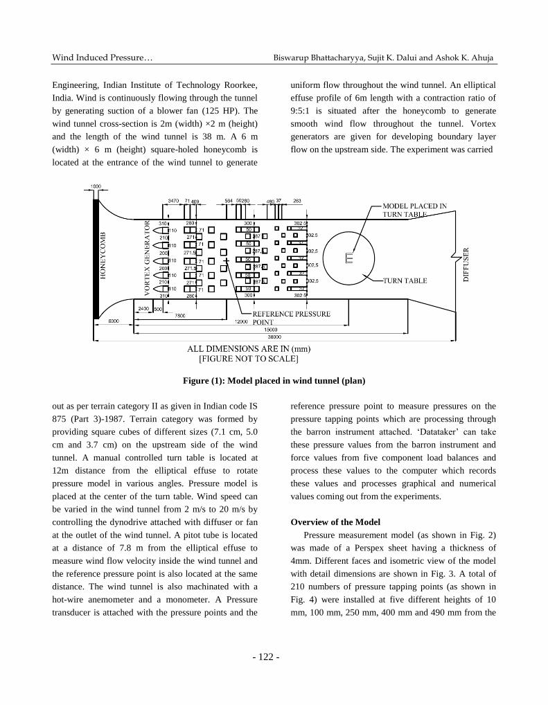
Experimental Setup

The experiments were conducted in an open circuit

boundary layer wind tunnel (as shown in Fig. 1) at

Wind Engineering Centre, Department of Civil

Wind Induced Pressure… Biswarup Bhattacharyya, Sujit K. Dalui and Ashok K. Ahuja

- 122 -

Engineering, Indian Institute of Technology Roorkee,

India. Wind is continuously flowing through the tunnel

by generating suction of a blower fan (125 HP). The

wind tunnel cross-section is 2m (width) ×2 m (height)

and the length of the wind tunnel is 38 m. A 6 m

(width) × 6 m (height) square-holed honeycomb is

located at the entrance of the wind tunnel to generate

uniform flow throughout the wind tunnel. An elliptical

effuse profile of 6m length with a contraction ratio of

9:5:1 is situated after the honeycomb to generate

smooth wind flow throughout the tunnel. Vortex

generators are given for developing boundary layer

flow on the upstream side. The experiment was carried

Figure (1): Model placed in wind tunnel (plan)

out as per terrain category II as given in Indian code IS

875 (Part 3)-1987. Terrain category was formed by

providing square cubes of different sizes (7.1 cm, 5.0

cm and 3.7 cm) on the upstream side of the wind

tunnel. A manual controlled turn table is located at

12m distance from the elliptical effuse to rotate

pressure model in various angles. Pressure model is

placed at the center of the turn table. Wind speed can

be varied in the wind tunnel from 2 m/s to 20 m/s by

controlling the dynodrive attached with diffuser or fan

at the outlet of the wind tunnel. A pitot tube is located

at a distance of 7.8 m from the elliptical effuse to

measure wind flow velocity inside the wind tunnel and

the reference pressure point is also located at the same

distance. The wind tunnel is also machinated with a

hot-wire anemometer and a monometer. A Pressure

transducer is attached with the pressure points and the

reference pressure point to measure pressures on the

pressure tapping points which are processing through

the barron instrument attached. ‘Datataker’ can take

these pressure values from the barron instrument and

force values from five component load balances and

process these values to the computer which records

these values and processes graphical and numerical

values coming out from the experiments.

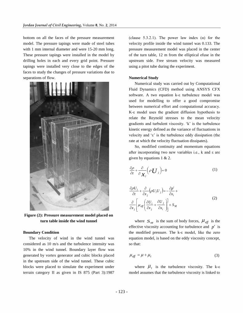
Overview of the Model

Pressure measurement model (as shown in Fig. 2)

was made of a Perspex sheet having a thickness of

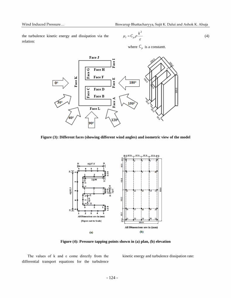
4mm. Different faces and isometric view of the model

with detail dimensions are shown in Fig. 3. A total of

210 numbers of pressure tapping points (as shown in

Fig. 4) were installed at five different heights of 10

mm, 100 mm, 250 mm, 400 mm and 490 mm from the


- 123 -

bottom on all the faces of the pressure measurement

model. The pressure tapings were made of steel tubes

with 1 mm internal diameter and were 15-20 mm long.

These pressure tapings were installed in the model by

drilling holes in each and every grid point. Pressure

tapings were installed very close to the edges of the

faces to study the changes of pressure variations due to

separations of flow.

Figure (2): Pressure measurement model placed on

turn table inside the wind tunnel

Boundary Condition

The velocity of wind in the wind tunnel was

considered as 10 m/s and the turbulence intensity was

10% in the wind tunnel. Boundary layer flow was

generated by vortex generator and cubic blocks placed

in the upstream side of the wind tunnel. These cubic

blocks were placed to simulate the experiment under

terrain category II as given in IS 875 (Part 3):1987

(clause 5.3.2.1). The power law index (α) for the

velocity profile inside the wind tunnel was 0.133. The

pressure measurement model was placed in the center

of the turn table, 12 m from the elliptical efuse in the

upstream side. Free stream velocity was measured

using a pitot tube during the experiment.

Numerical Study

Numerical study was carried out by Computational

Fluid Dynamics (CFD) method using ANSYS CFX

software. A two equation k-ε turbulence model was

used for modelling to offer a good compromise

between numerical effort and computational accuracy.

K-ε model uses the gradient diffusion hypothesis to

relate the Reynold stresses to the mean velocity

gradients and turbulent viscosity. ‘k’ is the turbulence

kinetic energy defined as the variance of fluctuations in

velocity and ‘ε’ is the turbulence eddy dissipation (the

rate at which the velocity fluctuation dissipates).

So, modified continuity and momentum equations

after incorporating two new variables i.e., k and ε are

given by equations 1 & 2.

0

U

x j

jt

(1)

Mi

j

j

ieff

j

iji

j

i

Sx

U

x

U

x

x

pUU

xt

U

(2)

where MS is the sum of body forces, eff is the

effective viscosity accounting for turbulence and p is

the modified pressure. The k-ε model, like the zero

equation model, is based on the eddy viscosity concept,

so that:

teff (3)

where t is the turbulence viscosity. The k-ε

model assumes that the turbulence viscosity is linked to


- 124 -

the turbulence kinetic energy and dissipation via the

relation:

2kCt (4)

where C is a constantt.

Figure (3): Different faces (showing different wind angles) and isometric view of the model

Figure (4): Pressure tapping points shown in (a) plan, (b) elevation

The values of k and ε come directly from the

differential transport equations for the turbulence

kinetic energy and turbulence dissipation rate:


- 125 -

kbk

jk

t

jj

j

PP

x

k

xkU

xt

k

(5)

)( 121 bk

j

t

jj

j

PCCPCk

xxU

xt

(6)

Pk is the turbulence production due to viscous

forces, which is modeled using:

kx

U

x

U

x

U

x

U

x

UP

k

kt

k

k

j

i

i

j

j

itk

33

2

(7)

C is k-ε turbulence model constant with the value

0.09. 1C , 2C are also k-ε turbulence model

constants in ANSYS CFX with values of 1.44 and

1.92, respectively. k is the turbulence model constant

for k equation with the value of 1.0 and is the

turbulence model constant for ε equation with the value

of 1.3. ρ is the density of air in ANSYS CFX taken as

1.224 kg/m3. Μ and μt are dynamic and turbulent

viscosity, respectively. The other notations have their

usual meanings. The building was considered as bluff

body in ANSYS CFX and the flow pattern around the

building was studied. Turbulence intensity was

considered as 10%.

Domain and Meshing

The domain size was taken as referred to by Revuz

et al. (2012). The upstream side was taken as 5H from

the face of the building, downstream side was taken as

15H from the face of the building, two side distance of

the domain was taken as 5H from the face of the

building and top clearance was taken as 5H from the

top surface of the building. Such large size of

downstream side helps in vortex generation in the

leeward side of the flow and backflow of wind is also

prevented. Multizone meshing and tetrahedron

meshing were conducted throughout the domain with a

hexagonal mesh and a tetrahedron mesh (Fig. 5),

respectively. Finer hexegonal and tetrahedron meshes

are very useful for generating uniform flow of wind

throughout the domain so that seperation of flow is

very smooth.

Figure (5): Mesh pattern around

the building model (plan)

Flowing Criteria

The boundary conditions were taken as the same in

the wind tunnel test such that the results found from the

experiment can validate the results obtained from the

numerical analysis.

Boundary layer wind flow near the windward side

was generated in the inlet of the domain using power

law:

00 z

z

U

U (8)

where U0 is the basic wind speed taken as 10 m/s,

Z0 is the boundary layer height considered 1 m as the


- 126 -

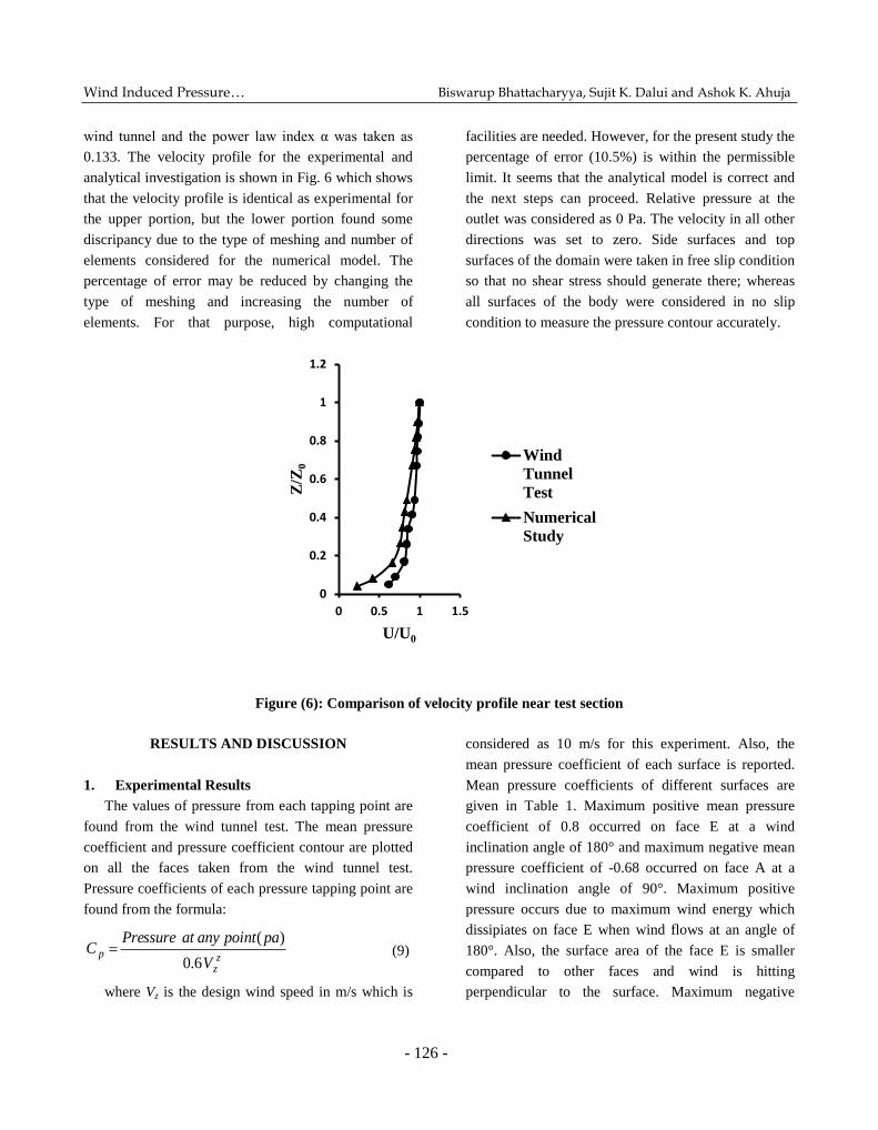
wind tunnel and the power law index α was taken as

0.133. The velocity profile for the experimental and

analytical investigation is shown in Fig. 6 which shows

that the velocity profile is identical as experimental for

the upper portion, but the lower portion found some

discripancy due to the type of meshing and number of

elements considered for the numerical model. The

percentage of error may be reduced by changing the

type of meshing and increasing the number of

elements. For that purpose, high computational

facilities are needed. However, for the present study the

percentage of error (10.5%) is within the permissible

limit. It seems that the analytical model is correct and

the next steps can proceed. Relative pressure at the

outlet was considered as 0 Pa. The velocity in all other

directions was set to zero. Side surfaces and top

surfaces of the domain were taken in free slip condition

so that no shear stress should generate there; whereas

all surfaces of the body were considered in no slip

condition to measure the pressure contour accurately.

Figure (6): Comparison of velocity profile near test section

RESULTS AND DISCUSSION

1. Experimental Results

The values of pressure from each tapping point are

found from the wind tunnel test. The mean pressure

coefficient and pressure coefficient contour are plotted

on all the faces taken from the wind tunnel test.

Pressure coefficients of each pressure tapping point are

found from the formula:

zz

pV

paintpoanyatessurePrC

6.0

)( (9)

where Vz is the design wind speed in m/s which is

considered as 10 m/s for this experiment. Also, the

mean pressure coefficient of each surface is reported.

Mean pressure coefficients of different surfaces are

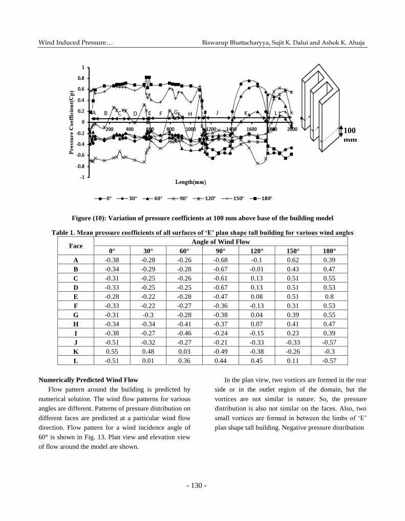
given in Table 1. Maximum positive mean pressure

coefficient of 0.8 occurred on face E at a wind

inclination angle of 180° and maximum negative mean

pressure coefficient of -0.68 occurred on face A at a

wind inclination angle of 90°. Maximum positive

pressure occurs due to maximum wind energy which

dissipiates on face E when wind flows at an angle of

180°. Also, the surface area of the face E is smaller

compared to other faces and wind is hitting

perpendicular to the surface. Maximum negative

0

0.2

0.4

0.6

0.8

1

1.2

0 0.5 1 1.5

Z/Z

0

U/U0

Wind

Tunnel

Test

Numerical

Study


- 127 -

pressure occurs on face A at an angle of 90° due to the

seperation of wind flow and high suction force occurs

on this face. Almost zero mean pressure coefficient

occurs on face B (-0.01), G (0.04) at a wind flow angle

of 120° and on face L (0.01) at a wind flow angle of

30°. In spite of zero mean pressure, the designer should

be more careful about the structural design because

almost equal portions or equal intensities of positive

and negative pressure occurred on these faces.

Generally, the structural elements of the faces of any

building are designed by considering mean pressure

coefficients, but it is better to consider node to node

variation of pressure coefficient in critical condition.

This will protect the building from wind desasters as

well as being economically cheaper than mean pressure

coefficient.

Pressure contours of all faces for 0° wind incidence

angle are shown in Fig. 7. Pattern of pressure contour

on face K is symmetrical about the vertical axis as the

wind is hitting perpendicularly on the surface of the

building. Also, the pressure contours of symmetrical

faces about vertical axis are also similar. Maximum

negative pressure (mean pressure coefficient of -0.51)

for 0° angle of wind flow occurred on two side faces

(face J and face L) due to high suction force in the

wind flow seperation zone. Negative pressure occurred

on all other faces of ‘E’ plan shape tall building.

Variations of pressure coefficient along the

horizontal centerline, 100 mm below the topmost fiber

of the building and 100 mm above the base of the

building, are also plotted for detailed investigation.

This will give the idealized pattern of pressure

coefficient throughout all the faces of the ‘E’ plan

shape tall building for various wind induced angles.

The variations of pressure coefficinet along the

horizontal centerline for all wind induced angles are

shown in Fig. 8. This Figure shows that variations of

pressure coefficinet for 0° and 180° are almost equal

and opposite in nature bacause flow directions are also

opposite. It is seen from Fig. 8 that pressure coefficient

fluctuates from negative to positive with almost the

same intensity from face A to face I at 120° angle of

wind attack, so the mean pressure coefficients of these

faces are almost zero or near to zero. This happened

due to the formation of irregular vortex caused by the

seperation of flow by the faces A, E and I. The effect of

each seperation is influencing the other and the

dynamic effect of wind is developing due to multi-

seperation. Also, two vortices are generated in between

the limbs of ‘E’ plan shape tall building.

The variations of pressure coefficient at the level of

100 mm from the top of the building and 100 mm from

the bottom of the building are plotted in Fig. 9 and Fig.

10, respectively for 0° to 180° angles of wind flow.

The variation of pressure coefficient is different from

the previous one (horizontal centerline). It is observed

that maximum positive pressure occurred on face E in

the case of a wind induced angle of 180° at the level of

100 mm from the top of the building. Almost equal

pressure is found from face A to face I for wind

induced angles of 0°, 30° and 60° because of the rear

side position with respect to the direction of wind flow.

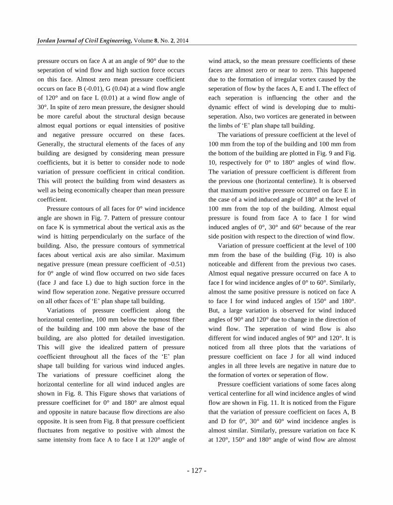
Variation of pressure coefficient at the level of 100

mm from the base of the building (Fig. 10) is also

noticeable and different from the previous two cases.

Almost equal negative pressure occurred on face A to

face I for wind incidence angles of 0° to 60°. Similarly,

almost the same positive pressure is noticed on face A

to face I for wind induced angles of 150° and 180°.

But, a large variation is observed for wind induced

angles of 90° and 120° due to change in the direction of

wind flow. The seperation of wind flow is also

different for wind induced angles of 90° and 120°. It is

noticed from all three plots that the variations of

pressure coefficient on face J for all wind induced

angles in all three levels are negative in nature due to

the formation of vortex or seperation of flow.

Pressure coefficient variations of some faces along

vertical centerline for all wind incidence angles of wind

flow are shown in Fig. 11. It is noticed from the Figure

that the variation of pressure coefficient on faces A, B

and D for 0°, 30° and 60° wind incidence angles is

almost similar. Similarly, pressure variation on face K

at 120°, 150° and 180° angle of wind flow are almost


- 128 -

similar. The variation of pressure coefficients along the

vertical centerline on faces B and D is almost equal for

all wind incidence angles. Similarities occurred due to

equal and opposite faces and wind flow equally

affected the faces.

Figure (7): Pressure contour on different surfaces of the model (Experimental Study/ Wind Tunnel test); (a) Face

K, (b) Faces J & L, (c) Faces A & I, (d) Faces B &H, (e) Faces D & F, (f) Faces C & G, (g) Face E

2. Numerical Results

Mean pressure coefficients of all the faces are also

found from numerical analysis using ANSYS CFX

software package with k-ε turbulence model. The mean

pressure coefficients of some of the faces for various

angles of wind flow are given in Table 2 with

experimental results to validate the numerical results.

Pressure contours of all faces for 0° wind incidence

angle are shown in Fig. 12.

From Table 2, it is seen that mean pressure

coefficients calculated by numerical methods are

within the reliable limit with respect to the


- 129 -

experimental values. Highest percentage of error

occurred on face J with 15.15% for 120° wind angle

whereas minimum percentage of error occurred on face

L with 1% for 30° wind angle. Mean pressure

coefficients of other surfaces are also given for

different wind angles in Table 2 and these values are

almost submerging with the experimental values.

Pressure contour plots on all faces for 0° wind

angle are also similar to those of experimental plots.

Pressure contours for different faces compared with

experimental results. Mean pressure coefficients of

these surfaces are also within the reliable limit with

respect to the experimental results.

Figure (8): Variation of pressure coefficients along horizontal centerline

Figure (9): Variation of pressure coefficients at 100 mm below top of the building model

400

mm

250

mm


- 130 -

Figure (10): Variation of pressure coefficients at 100 mm above base of the building model

Table 1. Mean pressure coefficients of all surfaces of ‘E’ plan shape tall building for various wind angles

Face Angle of Wind Flow

0° 30° 60° 90° 120° 150° 180°

A -0.38 -0.28 -0.26 -0.68 -0.1 0.62 0.39

B -0.34 -0.29 -0.28 -0.67 -0.01 0.43 0.47

C -0.31 -0.25 -0.26 -0.61 0.13 0.51 0.55

D -0.33 -0.25 -0.25 -0.67 0.13 0.51 0.53

E -0.28 -0.22 -0.28 -0.47 0.08 0.51 0.8

F -0.33 -0.22 -0.27 -0.36 -0.13 0.31 0.53

G -0.31 -0.3 -0.28 -0.38 0.04 0.39 0.55

H -0.34 -0.34 -0.41 -0.37 0.07 0.41 0.47

I -0.38 -0.27 -0.46 -0.24 -0.15 0.23 0.39

J -0.51 -0.32 -0.27 -0.21 -0.33 -0.33 -0.57

K 0.55 0.48 0.03 -0.49 -0.38 -0.26 -0.3

L -0.51 0.01 0.36 0.44 0.45 0.11 -0.57

Numerically Predicted Wind Flow

Flow pattern around the building is predicted by

numerical solution. The wind flow patterns for various

angles are different. Patterns of pressure distribution on

different faces are predicted at a particular wind flow

direction. Flow pattern for a wind incidence angle of

60° is shown in Fig. 13. Plan view and elevation view

of flow around the model are shown.

In the plan view, two vortices are formed in the rear

side or in the outlet region of the domain, but the

vortices are not similar in nature. So, the pressure

distribution is also not similar on the faces. Also, two

small vortices are formed in between the limbs of ‘E’

plan shape tall building. Negative pressure distribution

100

mm


- 131 -

Figure (11): Variation of pressure coefficients along vertical centerline of (a) Face A, (b) Face B,

(c) Face D, (d) Face K

Table 2. Comparison of mean pressure coefficients between experimental and analytical studies

Angle of

wind flow Face

Mean Surface Pressure Coefficient Change in

magnitude w. r. t.

(experimental)

Remarks Experimental

Result

Numerical

Result

0° K 0.55 0.54 2%(Decrease)

Results are

within

acceptable

limits

30° L 0.01 0.00 1%(Decrease)

60° H -0.41 -0.37 9.75%(Decrease)

90° E -0.47 -0.4 14.89%(Decrease)

120° J -0.33 -0.28 15.15%(Decrease)

150° G 0.39 0.34 12.82%(Decrease)

180° B & H 0.47 0.50 6.38%(Increase)


- 132 -

Figure (12): Pressure contour on different surfaces of the model (Numerical Study/ k-ε model);

(a) Face K, (b) Faces J & L, (c) Faces A & I, (d) Faces B &H, (e) Faces D & F, (f) Faces C & G, (g) Face E

Figure (13): Flow pattern around the building model; (a) plan, (b) elevation


- 133 -

occurred on these faces due to suction force acting at

the vortices. Also, negative pressure occurred on face

A and face J due to seperation of wind flow and high

suction force acting at the edges by the seperation of

wind flow. Face K and face L experienced direct wind

force, so positive pressure occurred on these faces. The

intensity of formation of vortices is gradually

increasing in nature from bottom to top.

CONCLUSIONS

This paper described the variation of pressure on all

the surfaces of ‘E’ plan shape tall building for wind

angle varying from 0° to 180° at an interval of 30°.

Both experimental and numerical studies have been

conducted. The wind flow pattern around the building

model has been also presented using software package

ANSYS CFX. Key features observed from the study

are discussed below.

Maximum positive mean pressure coefficient (0.8)

occurred on face E for 180° wind angle and

maximum negative mean pressure coefficient

(-0.68) occurred on face A for 90° wind angle.

Variations of pressure coefficient along horizontal

and vertical centerline have been also studied.

Fluctuation of pressure coefficient from face A to

face I varies from negative to positive with almost

equal intensity, so almost zero mean pressure

coefficients occurred on these faces. Variations of

pressure coefficient on faces A, B and D are almost

equal for 0°, 30° and 60° wind angles through the

vertical centerline.

Variation of pressure coefficient at the level of 100

mm above base and 100 mm below top of the

building model was also studied. The pressure

variation was different from that of horizontal

centerline. Almost equal pressure coefficients

occurred on face A to face I for 0° to 60° wind

angle in both cases. But, maximum positive

pressure occurred on face E at the level of 100 mm

from the top of the building model. Pressure

variations on face J at all three horizontal levels are

negative for all wind incidence angles.

Mean pressure coefficients calculated numerically

using k-ε turbulence model (Table 2) were almost

the same as the experimental results. The

differences are within the reliable limit.

Patterns of pressure distribution on all faces for all

wind incidence angles are predicted through

observing wind flow patterns around the building

model.

Numerical results may vary for different meshing

properties and different meshing sizes.

Implementation of finer meshing sizes may be

helpful to minimize the errors, but it also needs

high mechanical configuration.

ACKNOWLEDGEMENT

The financial support of the experimental study by

Department of Science & Technology (DST), India is

greatly appreciated. The work was fully supported by

Wind Engineering Center (WEC) of IIT Roorkee,

Roorkee, India.

REFERENCES

Amin, J. A., and Ahuja, A. K. (2012). “Wind-Induced

Mean Interference Effects Between Two Closed

Spaced Buildings.” KSCE Journal of Civil

Engineering, 16 (1), 119-131.

ANSYS 14.5, “ANSYS, Inc.”, www.ansys.com

ASCE 7-02. (2002). Minimum Design Loads for Buildings

and Other Structures, American Society of Civil

Engineering, ASCE Standard, Second Edition, Reston,

Virginia.

AS/NZS 1170.2: 2002. (2002). Structural Design Action,

Part 2: Wind Actions, Australian/ New-Zealand

Standard, Sydney, Wellington.


- 134 -

BS 6399-2: 1997. (1997). Loading for Buildings- Part 2:

Code of Practice for Wind Loads, British Standard,

London, UK.

Chakraborty, S., Dalui, S. K., and Ahuja, A. K. (2013).

“Experimental and Numerical Study of Surface

Pressure on ‘+’ Plan Shape Tall Building.”

International Journal of Construction Materials and

Structures, 1 (1), 45-58.

Chakraborty, S., and Dalui, S. K. (2013). “Numerical

Study of Surface Pressure on Square Plan Shape Tall

Building.” Symposium on Sustainable Infrastructure

Development (SID), February 8th to 9

th, 252-258, IIT

Bhubaneswar, Bhubaneswar, Odisha, India.

Fu, J. Y., Li, Q. S., Wu, J. R., Xiao, Y. Q., and Song, L. L.

(2008). “Field Measurements of Boundary Layer Wind

Characteristics and Wind-induced Responses of Super-

tall Buildings.” Journal of Wind Engineering and

Industrial Aerodynamics, 96 (8-9), 1332-1358.

Gomes, M. G., Rodrigues, A. M., and Mendes, P. (2005).

“Experimental and Numerical Study of Wind Pressures

on Irregular Plan Shapes.” Journal of Wind

Engineering and Industrial Aerodynamics, 93 (10),

741-756.

IS: 875 (Part 3). (1987). Indian Standard Code of Practice

for Design Wind Load on Buildings and Structures,

Second Revision, New Delhi, India.

Mendis, P., Ngo, T., Haritos, N., Hira, A., Samali, B., and

Cheung, J. (2007). “Wind Loading on Tall Buildings.”

Electronic Journal of Structural Engineering, EJSE

Special Issue: Loading on Structures, 41-54.

Revuz, J., Hargreaves, D. M., and Owen, J. S. (2012). “On

the Domain Size for the Steady State CFD Modelling

of a Tall Building.” Wind and Structures, 15 (4), 313-

329.

Tanaka, H., Tamura, Y., Ohtake, K., Nakai, M., and Kim,

Y. C. (2012). “Experimental Investigation of

Aerodynamic Forces and Wind Pressures Acting on

Tall Buildings with Various Unconventional

Configurations.” Journal of Wind Engineering and

Industrial Aerodynamics, 107-108, 179-191.

Wind Induced Pressure on ‘E’ Plan Shaped Tall Buildings

Documents

Transcript of Wind Induced Pressure on ‘E’ Plan Shaped Tall Buildings