Win-Stay, Lose-Sample: A simple sequential algorithm for ...alisongopnik.com/Papers_Alison/Bonawitz...

Cognitive Psychology 74 (2014) 35–65

Contents lists available at ScienceDirect

Cognitive Psychology

journal homepage: www.elsevier .com/locate/cogpsych

Win-Stay, Lose-Sample: A simple sequentialalgorithm for approximating Bayesian inference

http://dx.doi.org/10.1016/j.cogpsych.2014.06.0030010-0285/� 2014 Elsevier Inc. All rights reserved.

⇑ Corresponding author. Address: 334 Smith Hall, Department of Psychology, Rutgers University – Newark, Newark, NUSA.

E-mail address: [email protected] (E. Bonawitz).

Elizabeth Bonawitz a,⇑, Stephanie Denison b, Alison Gopnik c,Thomas L. Griffiths c

a Department of Psychology, Rutgers University – Newark, Newark, NJ USAb Department of Psychology, University of Waterloo, Waterloo, ON Canadac Department of Psychology, University of California, Berkeley, USA

a r t i c l e i n f o a b s t r a c t

Article history:Accepted 27 June 2014Available online 1 August 2014

Keywords:Bayesian inferenceAlgorithmic levelCausal learning

People can behave in a way that is consistent with Bayesian modelsof cognition, despite the fact that performing exact Bayesian infer-ence is computationally challenging. What algorithms could peo-ple be using to make this possible? We show that a simplesequential algorithm ‘‘Win-Stay, Lose-Sample’’, inspired by theWin-Stay, Lose-Shift (WSLS) principle, can be used to approximateBayesian inference. We investigate the behavior of adults and pre-schoolers on two causal learning tasks to test whether peoplemight use a similar algorithm. These studies use a ‘‘mini-microge-netic method’’, investigating how people sequentially update theirbeliefs as they encounter new evidence. Experiment 1 investigatesa deterministic causal learning scenario and Experiments 2 and 3examine how people make inferences in a stochastic scenario.The behavior of adults and preschoolers in these experiments isconsistent with our Bayesian version of the WSLS principle. Thisalgorithm provides both a practical method for performing Bayes-ian inference and a new way to understand people’s judgments.

� 2014 Elsevier Inc. All rights reserved.

J 07102,

http://crossmark.crossref.org/dialog/?doi=10.1016/j.cogpsych.2014.06.003&domain=pdf

http://dx.doi.org/10.1016/j.cogpsych.2014.06.003

mailto:[email protected]


http://www.sciencedirect.com/science/journal/00100285

http://www.elsevier.com/locate/cogpsych

36 E. Bonawitz et al. / Cognitive Psychology 74 (2014) 35–65

1. Introduction

In the last decade a growing literature has demonstrated that both adults and preschool childrencan act in ways that are consistent with the predictions of Bayesian models in appropriate contexts(e.g., Griffiths & Tenenbaum, 2005, 2009; Goodman, Tenenbaum, Feldman, & Griffiths, 2008; Gopnik& Schulz, 2004; Gopnik et al., 2004). Bayesian models provide a framework for more precisely charac-terizing intuitive theories, and they indicate how a rational learner should update her beliefs as sheencounters new evidence. The Bayesian approach has been used to explain the inferences adults makeabout causal relationships, words, and object properties (for a review see Tenenbaum, Griffiths, &Kemp, 2006; for critiques of this approach and responses, Jones & Love, 2011; Chater et al., 2011;Bowers & Davis, 2012; Griffiths, Chater, Norris, & Pouget, 2012; McClelland et al., 2010; Griffithset al., 2010). The approach can also explain the inferences that children make in these domains (forreviews see Gopnik, 2012; Gopnik & Wellman, 2012; Xu and Kushnir, 2012). Taken together, thesefindings suggest that Bayesian inference may provide a productive starting point for understandinghuman learning in these domains.

Bayesian models have typically been used to give a ‘‘computational level’’ analysis of the inferencespeople make when they solve inductive problems (Marr, 1982). That is, they focus on the form of thecomputational problem and its ideal solution. Bayesian models are concerned with the computationalproblem of how a learner should update her beliefs given new evidence. The ideal Bayesian solutionselects the most likely hypothesis after taking the evidence into account. However, it is extremelyunlikely that people are performing exact Bayesian inference at the algorithmic level as such inferencescan be extremely computationally challenging (e.g., Russell & Norvig, 2003). In particular, it would becomputationally costly to always enumerate and search through all the hypotheses that might becompatible with a particular pattern of evidence. Indeed, it has been generally acknowledged sincethe pioneering work of Simon (1955, 1957) that human cognition is at best ‘‘boundedly rational’’.

We might expect that rather than explicitly performing Bayesian inference, adults and children use‘‘fast and frugal’’ heuristics (Gigerenzer & Gaissmaier, 2011; Gigerenzer & Goldstein, 1996) thatapproximate Bayesian inference. Such heuristic procedures might lead to apparently irrationalinferences when considered step by step, even though in the long run those inferences would leadto a rational solution. An algorithmic account of learning could help explain both how people mightproduce inferences that can approximate rational models and why their step-by-step learningbehavior might appear irrational or protracted.

Thus, algorithmic accounts should approximate Bayesian inference, but they also need to becomputationally efficient. The need for efficiency is particularly important when we consider chil-dren’s learning. Young children have particularly limited cognitive resources, at least in some respects(e.g., German & Nichols, 2003; Gerstadt, Hong, & Diamond, 1994; Siegler, 1975), but are nonethelesscapable of behaving in a way that is consistent with optimal Bayesian models (Gopnik & Tenenbaum,2007). Children must thus be especially adept at managing limited resources to approximate Bayesianinference. At the same time, many of the most interesting cases of belief revision happen in the firstfew years of life (Bullock, Gelman, & Baillargeon, 1982; Carey, 1985; Gopnik & Meltzoff, 1997;Wellman, 1990). Understanding more precisely how existing beliefs and new evidence shapechildren’s learning given limited cognitive resources is a key challenge to proponents of Bayesianmodels of children’s cognition.

Here we investigate the algorithms that learners might be using to solve a particular kind of induc-tive problem – causal learning. Children learn a great deal about causal structure from very early indevelopment (e.g. Gopnik & Meltzoff, 1997; Gopnik & Schulz, 2007; Wellman & Gelman, 1992) andcausal knowledge and learning have been a particular focus of formal work in machine learningand philosophy of science (Pearl, 2000; Spirtes, Glymour, & Scheines, 2000). Causal learning has alsobeen one of the areas in which Bayesian models have been particularly effective in characterizinghuman behavior, from adults learning from contingency data (Griffiths & Tenenbaum, 2005) tochildren reasoning about causal systems and events (Bonawitz, Gopnik, Denison, & Griffiths, 2012;Bonawitz et al., 2011; Griffiths, Sobel, Tenenbaum, & Gopnik, 2011; Gweon, Schulz, & Tenenbaum,2010; Kushnir & Gopnik, 2007; Schulz, Bonawitz, & Griffiths, 2007; Seiver, Gopnik, & Goodman, 2012).

E. Bonawitz et al. / Cognitive Psychology 74 (2014) 35–65 37

Most studies of causal learning by children and adults simply relate the total amount ofevidence that a learner sees to the final inferences they make. This technique is well-suited toanalyzing the correspondence between the learner’s behavior and the predictions of computa-tional-level models. However, a more effective way to determine the actual algorithms that a lear-ner uses to solve these problems is to examine how her behavior changes, trial-by-trial, as newevidence is accumulated. We describe a new ‘‘mini-microgenetic’’ method (cf. Siegler, 1996) thatallows us to analyze the changes in a learner’s knowledge as she gradually accumulates newpieces of evidence. We can then compare this behavior to possible algorithmic approximationsof Bayesian inference.

Computer scientists and statisticians also face the challenge of finding efficient methods forperforming Bayesian inference. One common strategy for performing Bayesian inference is to useapproximations based on sampling, known as Monte Carlo methods. Under this strategy, computa-tions involving a probability distribution are conducted using samples from that distribution – anapproach that can be much more efficient. We introduce a new sequential sampling algorithm inspiredby the Win-Stay, Lose-Shift (WSLS) strategy,1 in which learners maintain a particular hypothesis untilthey receive evidence that is inconsistent with that hypothesis. We name our strategy Win-Stay, Lose-Sample to distinguish it from the original strategy. We show that our WSLS algorithm approximatesBayesian inference, and can do so more efficiently than enumerating hypotheses or performing simpleMonte Carlo search. Previous work in cognitive psychology demonstrates that people use a simple formof the Win-Stay, Lose-Shift strategy in concept learning tasks (Levine, 1975; Restle, 1962).

In previous experiments that compared human performance to the predictions of Bayesian models,researchers have typically looked at responses at just one point – after the evidence has been accumu-lated. In these tasks, the distribution of these responses often matches the posterior distribution thatwould be generated by Bayesian inference. That is, the proportion of people who endorse a particularhypothesis is closely related to the posterior probability of that hypothesis (e.g., Denison, Bonawitz,Gopnik, & Griffiths, 2013; Goodman et al., 2008; Vul, Goodman, Griffiths, & Tenenbaum, 2009; Xu &Tenenbaum, 2007; though, see also Bowers & Davis, 2012; Jones & Love, 2011; Marcus & Davis,2013). However, the psychological signature of WSLS algorithms is a characteristic pattern of depen-dency between people’s successive responses as the evidence comes in. In general terms, a learnerwho uses a WSLS algorithm will be ‘‘sticky’’; that is, they will show a tendency to prefer the hypothesiscurrently held to other possible hypotheses. What we demonstrate mathematically is that, despite anindividual’s tendency toward ‘‘stickiness’’, the overall proportion of individuals selecting a hypothesisat a given point in time will match the probability of that hypothesis given by Bayesian inference atthat point in time.

To test whether the signature pattern of dependence produced by our WSLS algorithm is presentin people’s judgments, we systematically compare this algorithm to an algorithm that uses indepen-dent sampling. In the independent sampling algorithm, the learner simply resamples a hypothesisfrom the new distribution yielded by Bayesian inference each time additional evidence is acquired.Independent sampling is similar to our WSLS algorithm in that it would also approximate thepredictions of a Bayesian model. However, by definition, it would not have the characteristic depen-dence between responses, as would WSLS. This contrast to independent sampling allows us to testsystematically whether learner’s responses are indeed dependent in the way that our WSLS algo-rithm would predict.

The plan for the rest of the paper is as follows. Next, we introduce the causal learning tasks that willbe the focus of our analysis and summarize how Bayesian inference can be applied in this task. Wethen introduce the idea of sequential sampling algorithms, including our new WSLS algorithm. Thisis followed by a mathematical analysis of the WSLS algorithm, showing that it approximates Bayesianinference in deterministic and non-deterministic cases. The remainder of the paper focuses on exper-iments in which we evaluate how well both Bayesian inference, in general, and the WSLS algorithm, inparticular, capture judgments by children and adults in two causal learning tasks in which the learnergradually acquires new evidence.

1 Also known as Win-Stay, Lose-Switch strategy (Robbins, 1952).


2. Analyzing sequential inductive inferences

While the algorithms that we present in this paper apply to any inductive problem with a discretehypothesis space, we will make our analysis concrete by focusing on two simple causal learningproblems, which are representative of the larger causal learning problems that children and adultsface. In the experiments that appear later in the paper we provide actual data from adults and childrensolving these problems, but we will begin by presenting a Bayesian computational analysis of howthese problems might be solved ideally. The first of these two problems involves deterministic events,and the second involves non-deterministic events, where object behavior is stochastic. The distinctivefeature of these learning problems is that participants are asked to provide predictions over multipletrials, as new evidence is observed. This allows us to model potential dependencies between an indi-vidual learner’s responses as her beliefs are updated following each successive piece of new evidence.

2.1. Deterministic events

Deterministic events provide a simple starting point for considering how a learner might updatehis or her beliefs. In the deterministic case the evidence a learner observes will necessarily rule outcertain hypotheses. As more and more evidence accumulates fewer hypotheses will remain.

For example, consider the following causal learning problem: there are two categories of objects(yellow and red blocks). Some of these blocks light up when they come into contact with other blocks.Blocks of the same color all behave similarly, and will either light or not light when they interact withother blocks. Given these constraints, we can generate a hypothesis space of 16 possible causalstructures, as illustrated in Fig. 1(a).

Using this hypothesis space, we can consider how an ideal learner should update his or her beliefsin light of evidence. Assume that the learner begins with a prior distribution over hypotheses, P(h),reflecting her degree of belief that each hypothesis is true before seeing any data. Given some

Fig. 1. A causal induction problem. (a) The sixteen possible hypotheses illustrated with the red (dark) and yellow (light) blocks;arrows indicate the causal direction of lighting. (b) The children’s prior distribution over the sixteen hypotheses. (c) The adult’sprior distribution over the sixteen hypotheses. (For interpretation of the references to color in this figure legend, the reader isreferred to the web version of this article.)


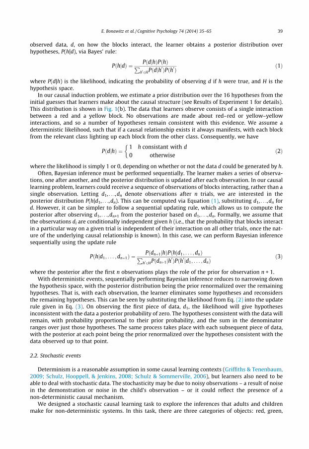
observed data, d, on how the blocks interact, the learner obtains a posterior distribution overhypotheses, P(h|d), via Bayes’ rule:

PðhjdÞ ¼ PðdjhÞPðhÞPh02HPðdjh0ÞPðh0Þ

ð1Þ

where P(d|h) is the likelihood, indicating the probability of observing d if h were true, and H is thehypothesis space.

In our causal induction problem, we estimate a prior distribution over the 16 hypotheses from theinitial guesses that learners make about the causal structure (see Results of Experiment 1 for details).This distribution is shown in Fig. 1(b). The data that learners observe consists of a single interactionbetween a red and a yellow block. No observations are made about red–red or yellow–yellowinteractions, and so a number of hypotheses remain consistent with this evidence. We assume adeterministic likelihood, such that if a causal relationship exists it always manifests, with each blockfrom the relevant class lighting up each block from the other class. Consequently, we have

PðdjhÞ ¼1 h consistant with d

0 otherwise

�ð2Þ

where the likelihood is simply 1 or 0, depending on whether or not the data d could be generated by h.Often, Bayesian inference must be performed sequentially. The learner makes a series of observa-

tions, one after another, and the posterior distribution is updated after each observation. In our causallearning problem, learners could receive a sequence of observations of blocks interacting, rather than asingle observation. Letting d1, . . .,dn denote observations after n trials, we are interested in theposterior distribution P(h|d1, . . .,dn). This can be computed via Equation (1), substituting d1, . . .,dn ford. However, it can be simpler to follow a sequential updating rule, which allows us to compute theposterior after observing d1, . . .,dn+1 from the posterior based on d1, . . .,dn. Formally, we assume thatthe observations di are conditionally independent given h (i.e., that the probability that blocks interactin a particular way on a given trial is independent of their interaction on all other trials, once the nat-ure of the underlying causal relationship is known). In this case, we can perform Bayesian inferencesequentially using the update rule

Pðhjd1; . . . ;dnþ1Þ ¼Pðdnþ1jhÞPðhjd1; . . . ;dnÞP

h02HPðdnþ1jh0ÞPðh0jd1; . . . ;dnÞð3Þ

where the posterior after the first n observations plays the role of the prior for observation n + 1.With deterministic events, sequentially performing Bayesian inference reduces to narrowing down

the hypothesis space, with the posterior distribution being the prior renormalized over the remaininghypotheses. That is, with each observation, the learner eliminates some hypotheses and reconsidersthe remaining hypotheses. This can be seen by substituting the likelihood from Eq. (2) into the updaterule given in Eq. (3). On observing the first piece of data, d1, the likelihood will give hypothesesinconsistent with the data a posterior probability of zero. The hypotheses consistent with the data willremain, with probability proportional to their prior probability, and the sum in the denominatorranges over just those hypotheses. The same process takes place with each subsequent piece of data,with the posterior at each point being the prior renormalized over the hypotheses consistent with thedata observed up to that point.

2.2. Stochastic events

Determinism is a reasonable assumption in some causal learning contexts (Griffiths & Tenenbaum,2009; Schulz, Hooppell, & Jenkins, 2008; Schulz & Sommerville, 2006), but learners also need to beable to deal with stochastic data. The stochasticity may be due to noisy observations – a result of noisein the demonstration or noise in the child’s observation – or it could reflect the presence of anon-deterministic causal mechanism.

We designed a stochastic causal learning task to explore the inferences that adults and childrenmake for non-deterministic systems. In this task, there are three categories of objects: red, green,


and blue blocks. Each of these kinds of blocks activates a machine with different probability when theyare placed on the machine. The red blocks activate the machine on five out of six trials, the greenblocks on three out of six trials, and the blue blocks on just one out of six trials. A new block is thenpresented that has lost its color and needs to be classified as either a red, green, or blue block. Thelearner observes what happens when the block is placed on the machine over a series of trials. Whatshould learners infer about the category and causal properties of this block as they gradually acquiremore evidence about its effects?

As with the deterministic case, given this hypothesis space, we can compute an ideal learner’sposterior distribution over hypotheses via Bayes’ rule (Eq. (1)). In this case, the likelihood takes ona wider range of values. If we take our data d to be the activation of the machine, the probability ofthis event depends on our hypothesis about the color of the block. For the red block, we might takeP(d|h) to be 5/6; for the green block, 3/6; and for the blue block, 1/6. Importantly, observing the blocklight up or not light up the detector no longer clearly rules out any of these hypotheses. Bayesian infer-ence thus becomes a matter of balancing the evidence provided by the data with our prior beliefs. Wecan still use the sequential updating rule given in Eq. (3), but now each new piece of data is only goingto steer us a little more toward one hypothesis or another.

2.3. Toward algorithms for Bayesian inference

This analysis of sequential causal learning in deterministic and nondeterministic scenarios allowsus to think about how learners should select hypotheses by combining prior beliefs with evidence.However, assuming that learners’ responses do reflect this optimal trade-off between priors andevidence, this analysis makes no commitments about the algorithms that might be used to approxi-mate Bayesian inference. In particular, it makes no commitments about how an individual learner willrespond to data, contingent on her previous guess, other than requiring that both responses beconsistent with the associated posterior distributions. Given a potentially large hypothesis space,searching through that space of hypotheses in a way that yields something approximating Bayesianinference is a challenge. In the remainder of the paper, we investigate how a learner might addressthis challenge.

3. Sequential sampling algorithms

The Bayesian analysis presented in the previous section provides an abstract, ‘‘computational level’’characterization of causal induction for these two causal learning tasks, identifying the underlyingproblem and how it might best be solved (Marr, 1982). We now turn to the problem of how to approx-imate this optimal solution.

One way a learner might compute an optimal solution is by simply following the recipe providedby Bayes’ rule. However, enumerating all hypotheses and then updating their probabilities bymultiplying prior and likelihood, quickly becomes computationally expensive. We thus consider thepossibility that people may be approximating Bayesian inference by following a procedure thatproduces samples from the posterior distribution.

3.1. Approximating Bayesian inference by sampling

Sophisticated Monte Carlo methods for approximating Bayesian inference developed in computerscience and statistics make it possible to draw a sample from the posterior without having to calculatethe full distribution (see, e.g., Robert & Casella, 2004). Thus, rather than having to evaluate every singlehypothesis and work through Bayes’ rule, these methods make it possible to consider only a fewhypotheses that have been sampled with the appropriate probabilities. These few hypotheses canbe evaluated using Bayes rule to generate samples from the posterior distribution. Aggregating overthese samples provides an approximation to the posterior distribution. That is, for approximatealgorithms, as the number of samples they generate increase, the distribution of samples convergesto the normative distribution. These sampling algorithms are consistent with behavioral evidence that


both adults and children select hypotheses in proportion to their posterior probability (Denison et al.,2013; Goodman et al., 2008).

Note that these sampling algorithms also address a conflict between rational models of cognitionand the finding that people show significant individual variability in responding (e.g. Siegler & Chen,1998). A system that uses this sort of sampling will be variable – it will entertain different hypothesesapparently at random from one time to the next. However, this variability will be systematicallyrelated to the probability distribution of the hypotheses, as more probable hypotheses will be sampledmore frequently than less probable ones. And, on aggregate, the distribution of hypotheses from manylearners (or one learner across multiple trials), will approximate the probability distribution. Recentresearch has explored this ‘‘Sampling Hypothesis’’ generally and suggested that the variability inyoung children’s responses may be part of a rational strategy for inductive inference (Bonawitz,Denison, Griffiths, & Gopnik, 2014; Denison et al., 2013).

The idea that people might be generating hypotheses by sampling from the posterior distributionstill leaves open the question of what kind of sampling scheme they might be using to update theirbeliefs. Independent Sampling (IS) is the simplest strategy, and is thus a parsimonious place to startconsidering the algorithms learners might use. In Independent Sampling, a learner would generatea sample from the posterior distribution independently each time one was needed. This can be doneusing a variety of Monte Carlo schemes such as importance sampling (see Neal, 1993, for details) andMarkov chain Monte Carlo (see Gilks, Richardson, & Spiegelhalter, 1996, for details). Such schemeshave previously been proposed as possible accounts of human cognition, (Shi, Feldman, & Griffiths,2008; Ullman, Goodman, & Tenenbaum, 2010). However, this approach can be inefficient in situationswhere the posterior distribution needs to be approximated repeatedly as more data become available.Independent Sampling requires that the system recompute the approximation to the posterior aftereach piece of data is observed.

People might adopt an alternative strategy that exploits the sequential structure of the problem ofupdating beliefs. The problem of sequentially updating a posterior distribution in light of evidence canbe solved approximately using sequential Monte Carlo methods such as particle filters (Doucet, deFreitas, & Gordon, 2001). A particle filter approximates the probability distribution over hypothesesat each point in time with a set of samples (or ‘‘particles’’), and provides a scheme for updating thisset to reflect the information provided by new evidence. The behavior of the algorithm depends onthe number of particles. With a very large number of particles, each particle is similar to a sample fromthe posterior. With a small number of particles, there can be strong sequential dependencies in therepresentation of the posterior distribution. Recent work has explored particle filters as a way toexplain patterns of sequential dependency that arise in human inductive inference (Levy, Reali, &Griffiths, 2009; Sanborn, Griffiths, & Navarro, 2010).

Particle filters have many degrees of freedom, and many different schemes for updating particlesare possible (Doucet et al., 2001). They also require learners to maintain multiple hypotheses at eachpoint in time. Here, we investigate a simpler algorithm that assumes that learners maintain a singlehypothesis, only occasionally resampling from the posterior and shifting to a new hypothesis. Thedecision to resample and so shift to a new hypothesis is probabilistic. The learner resamples with aprobability dependent on the degree to which the hypothesis is contradicted by data. As the probabil-ity of the sampled hypothesis given the data goes down, the learner is more likely to resample. This issimilar to using a particle filter with just a single particle. The computationally expensive resamplingstep is more likely to be carried out as that particle becomes inconsistent with the data. This algorithmtends to maintain a hypothesis that makes a successful prediction and only tries a new hypothesiswhen the data weigh against the original choice. Thus, this algorithm may have some advantages overother forms of Monte Carlo search that resample after every observation. The central idea ofmaintaining a hypothesis provided it successfully accounts for the observed data leads us to referto this strategy as the Win-Stay, Lose-Sample (WSLS) algorithm.

3.2. History of the WSLS principle

The WSLS principle has a long history in computer science and statistics, where it appears as aheuristic algorithm in reinforcement learning (Robbins, 1952). Robbins (1952) defined a heuristic


method for maximizing reward in a two-armed bandit problem based on this principle, in which anagent continues to perform an action provided that action is rewarded. These early studies employedvery specific types of WSLS procedures, but in fact, the principle falls under a more general class ofalgorithms that depend on decisions from experience (see Erev, Ert, Roth, et al., 2010, for a review).

The principle also has a long history in psychology. The basic principle of repeating behaviors thathave positive consequences and not performing behaviors that have negative consequences can betraced back to Thorndike (1911). Restle (1962) did not explicitly call his model a WSLS algorithm,but he proposed a simple model of human concept learning that employed a similar principle, inwhich people were assumed to hold a single hypothesis in mind about the nature of a concept, onlyrejecting that hypothesis (and drawing a new one at random) when they received inconsistent evi-dence. This model, however, assumed that people could not remember the hypotheses they had triedpreviously or the pattern of data that they had observed. In fact people do use this information inconcept learning, and Restle’s version of the WSLS algorithm was subsequently shown to be a poorcharacterization of human concept learning (Erikson, 1968; Trabasso & Bower, 1966).

A form of the WSLS strategy has also been shown to be used by children, most notably in proba-bility learning experiments using variable reinforcement schedules (Schusterman, 1963; Weir,1964). Schusterman (1963) asked children to complete a two-alternative choice task in which theycould obtain prizes by searching in one of two locations across many trials. Each location containedthe prize on 50% of the trials, but in one condition, the probability that a reward would appear on agiven side was 64% if the reward had occurred on that side in the previous trial, while in another con-dition, this probability was 39%. The three-year-olds very strongly followed a WSLS strategy, even inthe condition where this strategy would not maximize the reward (i.e., the 39% condition). The five-year-olds showed a more sophisticated pattern, using a WSLS strategy more often in the 64% than inthe 39% condition.

Weir (1964) also used a probability learning task to examine the development of hypothesis testingstrategies throughout childhood. Over many trials, a child had to choose to turn one of three knobs ona panel to obtain a marble. Only one knob produced marbles and it did so probabilistically (e.g., on 66%of the trials). Results were analyzed in terms of a variety of strategies, including WSLS. In this task, themost common pattern followed by three- to five-year-old children was a win-stay, lose-stay strategy,(i.e., persevering with the initial hypothesis) which maximizes reward in this task. The 7- to 15-year-old children were more likely than the other age groups to show a WSLS strategy, but children in thisage range also commonly used a win-shift, lose-shift (i.e., alternation) strategy.

A parallel form of WSLS has also been analyzed as a simple model of learning that leads tointeresting strategies in game theory, where it is often used to describe behavior in deterministic bin-ary decision tasks (see Colman, Pulford, Omtzigt, & al-Nowaihi, 2010, for a more complete historicaloverview). For example, Nowak and Sigmund (1993) showed that WSLS outperforms tit-for-tat(TFT) strategies in extended evolutionary simulations of the Prisoner’s Dilemma game when thesimulations include these additional complexities. The use of WSLS, as opposed to TFT, results in muchquicker recovery following errors and exploitation of unconditional cooperators – behaviors thatcorrespond well with typical decisions of both humans and other animals.

3.3. Analyzing the WSLS algorithm

The WSLS principle provides an intuitive strategy for updating beliefs about hypotheses over time.This raises the question of whether there are specific WSLS strategies that can actually approximatethe distribution over hypotheses that would be computed using full Bayesian inference. That is, arethere specific variants of WSLS that, like independent sampling, converge to the posterior distributionas the number of samples increase? These kinds of WSLS strategies would have to be more sophisti-cated than the simple strategies we have described so far.

In exploring the question of whether an algorithm based on the WSLS principle can approximateBayesian inference, we will also extend our analysis of WSLS to include cases where data areprobabilistic. Previous work discussing WSLS strategies would only allow for deterministic shifts fromone hypothesis to another. This involves a simple yes–no judgment about whether the data confirm orrefute a hypothesis. Bayesian inference, in contrast, is useful because it allows a learner to weight


evidence probabilistically. Can an algorithm that uses the basic WSLS principle, but includes moresophisticated kinds of probabilistic computation also be used to approximate Bayesian inference?

Our WSLS algorithm assumes that learners maintain their current hypothesis provided they seedata that are consistent with that hypothesis, and generate a new hypothesis otherwise. This is closestto the version explored by Restle (1962), but diverges from it in that instead of randomly choosing ahypothesis from an a priori equally weighted set of hypotheses (consistent with the data), a learnersamples a hypothesis from the posterior distribution. That is, the important difference between thesemodels is that in contrast to choosing a hypothesis at random from a stable, uniform distribution, inour model a learner chooses the next hypothesis with probability proportional to its posteriorprobability, which is continually being updated as new data are observed. The posterior distributionin deterministic cases is simply the prior distribution renormalized by the remaining consistenthypotheses.

It is relatively straightforward to show that this algorithm can approximate Bayesian inference incases where the likelihood function p(di|h) is deterministic, giving a probability of 1 or 0 to anyobservation di for every h, and observations are independent conditioned on hypotheses. More pre-cisely, the marginal probability of selecting a hypothesis hn given data, d1, . . .,dn, is the posterior prob-ability P(h|d1, . . .,dn), provided that the initial hypothesis is sampled from the prior distribution P(h)and hypotheses are sampled from the posterior distribution whenever the learner chooses to shifthypotheses.2 That is to say, like other approximation algorithms such as Independent Sampling, if youwere to look at the distribution of responses of a group of learners who observed the same evidenceand who were each following this WSLS strategy, the distribution of answers would approximate theposterior distribution predicted by Bayesian inference. This algorithm is thus a candidate for approximat-ing Bayesian inference in settings similar to the deterministic causal induction problem that we explorein this paper. The proof is given in Appendix A and provides the first of two specific WSLS algorithms thatwe will investigate.

More interestingly, the WSLS algorithm can be extended to approximate Bayesian inference instochastic settings by assuming that the probability of shifting hypotheses is determined by theprobability of the observed data under the current hypothesis. A proof of the more general case, forstochastic settings, is provided in Appendix B. The proof provides a simple set of conditions underwhich the probability that a learner following the WSLS algorithm entertains a particular hypothesismatches the posterior probability of that hypothesis. Essentially, when data are more consistent withthe current hypothesis we treat it as a ‘‘win’’; this means a learner is more likely to stay with herhypothesis. When data are less consistent with the hypothesis, we treat it as a ‘‘loss’’; this meansthe learner is more likely to sample from the updated posterior.

There are two interesting special cases of the class of WSLS algorithms identified by the conditionslaid out in our proof. The first special case is a simple algorithm that makes a choice to resample fromthe posterior based on the likelihood associated with the current observation di for the current h,p(di|h). With probability proportional to this likelihood, the learner maintains the current hypothesis;otherwise, she samples a new hypothesis from the posterior distribution. The second special case isthe most efficient algorithm of this kind, in the sense that it minimizes the rate at which samplingfrom the posterior is required. Resampling is minimized by considering the likelihood for the currenthypothesis relative to the likelihoods for all hypotheses when determining whether to resample – ifthe current hypothesis assigns highest probability to the current observation, then the learner willalways maintain that hypothesis. The proof demonstrates that following one of these algorithmsresults in the same overall aggregate result as learners always sampling a response from the updatedposterior, and thus approximates Bayesian inference. Our exploration of the WSLS algorithm instochastic settings will focus on the first of these cases, where the choice to resample is based juston the likelihood for the current hypothesis, as this minimizes the burden on the learner.

2 It is worth noting that the WSLS algorithm still requires the learner to generate samples from the posterior distribution.However, this algorithm is more efficient than Independent Sampling, since samples are only generated when the currenthypothesis is rejected. Other inference algorithms, such as Markov chain Monte Carlo, could be used at this point to sample fromthe posterior distribution without having to enumerate all hypotheses – a possibility we return to later in the paper.


Our WSLS algorithm differs in an important way from other variants of WSLS strategies whenused in a stochastic setting, in that it is possible that the learner ends up with the same hypothesisagain after ‘‘switching’’ (because that hypothesis is sampled from the posterior). This contrasts withvariants of the WSLS rule that require the learner to always shift to a new hypothesis (see Colmanet al., 2010). While such an algorithm would behave the same as our algorithm in a deterministicsetting if it was appropriately augmented to sample from the posterior on switching, it wouldbehave differently in a stochastic setting. It is an interesting open question whether this (potentiallymore efficient) ‘‘must switch’’ algorithm can be generalized to approximate Bayesian inference in astochastic setting.

Both Independent Sampling and WSLS can approximate the posterior distribution, but there is animportant difference between them: WSLS introduces dependencies between responses and favorssticking with the current hypothesis. We can characterize this difference formally as follows. In ISthere is no dependency between the hypotheses sampled after data points n and n + 1, hn and hn+1,but there is for WSLS: if the data are consistent with hn, then the learner will retain hn with probabilityproportional to p(d|hn) rather than randomly sampling hn+1 from the posterior distribution. We can usethis difference to attempt to diagnose whether people use a WSLS type algorithm when they aresolving a causal learning problem.

4. Evaluating inference strategies in children and adults

We now turn to the question of whether people’s actual responses are well captured by thealgorithms described in the previous section, which we explore using mini-microgenetic studies withboth adults and preschool children. Young children are a particularly important group to study for tworeasons. First, their responses are unlikely to be influenced by specific education or explicit training ininference. Second, if these inductive procedures are in place in young children, they could contributeto the remarkable amount of causal learning that takes place in childhood.

In particular, we explore children’s responses in a causal learning task in which they must judgewhether a particular artifact, such as a block, is likely to have particular effects, such as causing amachine or another block to light up. In earlier studies using very similar methods (e.g. ‘‘blicket detec-tor’’ studies) researchers have found that preschool children’s inferences go beyond simple associativelearning and have the distinctive profile of causal inferences. For example, children will use inferencesabout the causal relation of the block and machine to design novel interventions on the machine –patterns of action they have never actually observed – to construct counter-factual inferences andto make explicit causal judgments including judgments about unobserved hidden features of theobjects (e.g. Bonawitz, van Schindel, Friel, & Schulz, 2012; Gopnik & Sobel, 2000; Gopnik et al.,2004; Schulz, Gopnik, & Glymour, 2007; Sobel, Yoachim, Gopnik, Meltzoff, & Blumenthal, 2007).

Although in many contexts young learners demonstrate sophisticated casual reasoning, there arenumerous findings that children (and adults alike) have difficulty with explicit hypothesis testing(e.g., Klahr, Fay, & Dunbar, 1993; Kuhn, 1989). Although young children clearly can sometimesarticulate hypotheses explicitly, and can learn them from evidence, they have much more difficultyarticulating or judging how hypotheses are justified by evidence. Our task is designed to explorechildren’s and adults’ reasoning about a causal system, but does not require the learner to be meta-cognitively aware of their own process of reasoning from the data.

In each experiment, we first determine whether the responses of both adults and children in thesetasks are consistent with Bayesian inference at the computational level. Then we explore whethertheir behavior is consistent with particular learning algorithms, with special focus on the WSLSalgorithm and Independent Sampling. In particular, we might expect that if participants behave inways consistent with the WSLS algorithm we should observe dependencies between their responses.Experiment 1 begins with an empirical investigation of the deterministic causal learning scenario wedescribed earlier. Experiments 2 and 3 examine how people make inferences in the stochasticscenario.


5. Experiment 1: Deterministic causal learning

5.1. Methods

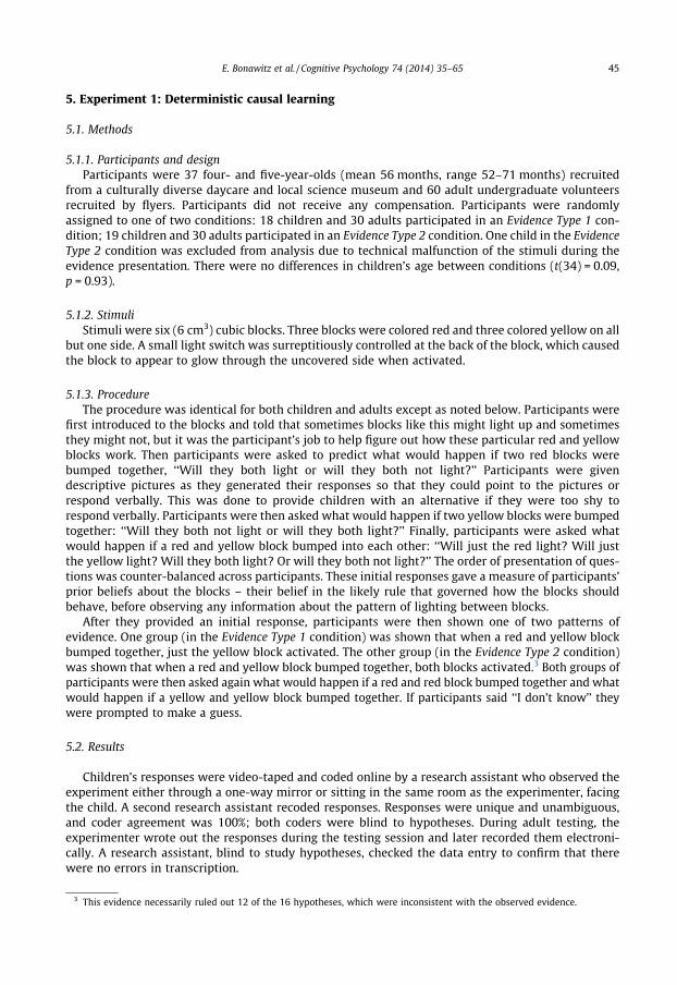
5.1.1. Participants and designParticipants were 37 four- and five-year-olds (mean 56 months, range 52–71 months) recruited

from a culturally diverse daycare and local science museum and 60 adult undergraduate volunteersrecruited by flyers. Participants did not receive any compensation. Participants were randomlyassigned to one of two conditions: 18 children and 30 adults participated in an Evidence Type 1 con-dition; 19 children and 30 adults participated in an Evidence Type 2 condition. One child in the EvidenceType 2 condition was excluded from analysis due to technical malfunction of the stimuli during theevidence presentation. There were no differences in children’s age between conditions (t(34) = 0.09,p = 0.93).

5.1.2. StimuliStimuli were six (6 cm3) cubic blocks. Three blocks were colored red and three colored yellow on all

but one side. A small light switch was surreptitiously controlled at the back of the block, which causedthe block to appear to glow through the uncovered side when activated.

5.1.3. ProcedureThe procedure was identical for both children and adults except as noted below. Participants were

first introduced to the blocks and told that sometimes blocks like this might light up and sometimesthey might not, but it was the participant’s job to help figure out how these particular red and yellowblocks work. Then participants were asked to predict what would happen if two red blocks werebumped together, ‘‘Will they both light or will they both not light?’’ Participants were givendescriptive pictures as they generated their responses so that they could point to the pictures orrespond verbally. This was done to provide children with an alternative if they were too shy torespond verbally. Participants were then asked what would happen if two yellow blocks were bumpedtogether: ‘‘Will they both not light or will they both light?’’ Finally, participants were asked whatwould happen if a red and yellow block bumped into each other: ‘‘Will just the red light? Will justthe yellow light? Will they both light? Or will they both not light?’’ The order of presentation of ques-tions was counter-balanced across participants. These initial responses gave a measure of participants’prior beliefs about the blocks – their belief in the likely rule that governed how the blocks shouldbehave, before observing any information about the pattern of lighting between blocks.

After they provided an initial response, participants were then shown one of two patterns ofevidence. One group (in the Evidence Type 1 condition) was shown that when a red and yellow blockbumped together, just the yellow block activated. The other group (in the Evidence Type 2 condition)was shown that when a red and yellow block bumped together, both blocks activated.3 Both groups ofparticipants were then asked again what would happen if a red and red block bumped together and whatwould happen if a yellow and yellow block bumped together. If participants said ‘‘I don’t know’’ theywere prompted to make a guess.

5.2. Results

Children’s responses were video-taped and coded online by a research assistant who observed theexperiment either through a one-way mirror or sitting in the same room as the experimenter, facingthe child. A second research assistant recoded responses. Responses were unique and unambiguous,and coder agreement was 100%; both coders were blind to hypotheses. During adult testing, theexperimenter wrote out the responses during the testing session and later recorded them electroni-cally. A research assistant, blind to study hypotheses, checked the data entry to confirm that therewere no errors in transcription.

3 This evidence necessarily ruled out 12 of the 16 hypotheses, which were inconsistent with the observed evidence.


To assess which theory each learner held during each stage of the experiment, we looked at thecausal judgments about each set of blocks interactions and selected the hypothesis consistent withparticipants’ predictions. For example, if the participant responded that two red blocks would lighteach other, two yellow blocks would not light each other, and a red block would light a yellow block(but not vice versa) then the response was coded as theory 2; see Fig. 1.

5.2.1. Prior distribution5.2.1.1. Children. Because the initial phase of the experiment was identical across conditions, wecombined the children’s responses in the initial phase to look at the overall prior distribution overhypotheses. Children had a slight bias for theories that included a greater number of positive, lightingrelations. For both IS and WSLS models we estimated an empirical prior from this initial distributionproduced by the children. The frequencies of each causal structure were tabulated from the children’sresponses. The relatively large number of causal structures to choose from compared to the number ofparticipants resulted in a few structures that were never produced. To minimize bias from thesesmaller sample sizes, smoothing was performed by adding 1 ‘‘observation’’ to each theory before nor-malizing, consistent with using a uniform Dirichlet prior on the multinomial distribution over causalstructures (e.g., Bishop, 2006). The smoothed estimated prior distribution over children’s hypothesesis shown in Fig. 1(b).

5.2.1.2. Adults. We also combined responses from both conditions in order to investigate the overallprior distribution over adults’ responses and tabulated frequencies adding 1 to all bins beforenormalizing. The estimated prior distribution over adult’s hypotheses is shown in Fig. 1(c).

5.2.2. Aggregate distributionWe then considered how responses would change when the learner received new evidence. We

computed the updated Bayesian posteriors for both conditions and for the children and the adults sep-arately using the prior distributions above. Comparing the proportion of participants who endorsedeach theory following the evidence to the Bayesian posterior distribution revealed high correlations(Children: r = .92; Adults: r = .97). So, at the computational level, the learners seemed to produceresponses that are consistent with Bayesian inference in this task. In the Evidence Type 1 conditionthere appears to be mild deviations between the model predictions and children’s endorsement ofTheory 10 and Theory 14; however, comparing the proportion of responses predicted by the Bayesianmodel for these theories to the proportion given by the children revealed no significant difference,v2 (1, N = 30) = 1.2, p = .27.

Fig. 2. Results of the Independent Sampling and Win-Stay, Lose-Sample algorithms, as compared to the Bayesian posterior andparticipant responses. (a) Predictions generated from children’s priors and children’s responses. (b) Predictions generated fromadult’s priors and adult’s responses. Dark bars represent the Evidence Type 1 and the lighter lines are Evidence Type 2.


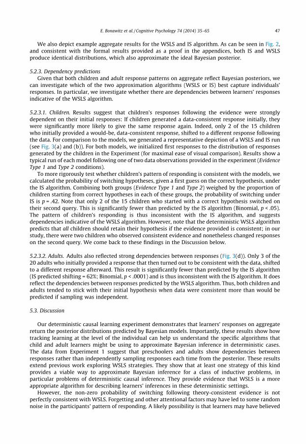
We also depict example aggregate results for the WSLS and IS algorithm. As can be seen in Fig. 2,and consistent with the formal results provided as a proof in the appendices, both IS and WSLSproduce identical distributions, which also approximate the ideal Bayesian posterior.

5.2.3. Dependency predictionsGiven that both children and adult response patterns on aggregate reflect Bayesian posteriors, we

can investigate which of the two approximation algorithms (WSLS or IS) best capture individuals’responses. In particular, we investigate whether there are dependencies between learners’ responsesindicative of the WSLS algorithm.

5.2.3.1. Children. Results suggest that children’s responses following the evidence were stronglydependent on their initial responses: If children generated a data-consistent response initially, theywere significantly more likely to give the same response again. Indeed, only 2 of the 15 childrenwho initially provided a would-be, data-consistent response, shifted to a different response followingthe data. For comparison to the models, we generated a representative depiction of a WSLS and IS run(see Fig. 3(a) and (b)). For both models, we initialized first responses to the distribution of responsesgenerated by the children in the Experiment (for maximal ease of visual comparison). Results show atypical run of each model following one of two data observations provided in the experiment (EvidenceType 1 and Type 2 conditions).

To more rigorously test whether children’s pattern of responding is consistent with the models, wecalculated the probability of switching hypotheses, given a first guess on the correct hypothesis, underthe IS algorithm. Combining both groups (Evidence Type 1 and Type 2) weighed by the proportion ofchildren starting from correct hypotheses in each of these groups, the probability of switching underIS is p = .42. Note that only 2 of the 15 children who started with a correct hypothesis switched ontheir second query. This is significantly fewer than predicted by the IS algorithm (Binomial, p < .05).The pattern of children’s responding is thus inconsistent with the IS algorithm, and suggestsdependencies indicative of the WSLS algorithm. However, note that the deterministic WSLS algorithmpredicts that all children should retain their hypothesis if the evidence provided is consistent; in ourstudy, there were two children who observed consistent evidence and nonetheless changed responseson the second query. We come back to these findings in the Discussion below.

5.2.3.2. Adults. Adults also reflected strong dependencies between responses (Fig. 3(d)). Only 3 of the20 adults who initially provided a response that then turned out to be consistent with the data, shiftedto a different response afterward. This result is significantly fewer than predicted by the IS algorithm(IS predicted shifting = 62%; Binomial, p < .0001) and is thus inconsistent with the IS algorithm. It doesreflect the dependencies between responses predicted by the WSLS algorithm. Thus, both children andadults tended to stick with their initial hypothesis when data were consistent more than would bepredicted if sampling was independent.

5.3. Discussion

Our deterministic causal learning experiment demonstrates that learners’ responses on aggregatereturn the posterior distributions predicted by Bayesian models. Importantly, these results show howtracking learning at the level of the individual can help us understand the specific algorithms thatchild and adult learners might be using to approximate Bayesian inference in deterministic cases.The data from Experiment 1 suggest that preschoolers and adults show dependencies betweenresponses rather than independently sampling responses each time from the posterior. These resultsextend previous work exploring WSLS strategies. They show that at least one strategy of this kindprovides a viable way to approximate Bayesian inference for a class of inductive problems, inparticular problems of deterministic causal inference. They provide evidence that WSLS is a moreappropriate algorithm for describing learners’ inferences in these deterministic settings.

However, the non-zero probability of switching following theory-consistent evidence is notperfectly consistent with WSLS. Forgetting and other attentional factors may have led to some randomnoise in the participants’ pattern of responding. A likely possibility is that learners may have believed

Fig. 3. Predictions of both models with priors generated from children’s initial predictions, compared against human judgments(a) Independent Sampling, and (b) Win-Stay, Lose-Sample, and (c) children’s responses. Models with priors generated fromadults’ initial predictions (d) Independent Sampling, and (e) Win-Stay, Lose-Sample, and (f) adults’ responses. Dark linesrepresent the data observation of a red and yellow block interacting and resulting in just the yellow block lighting, leaving onlyhypotheses 2, 6, 10, and 14 consistent with the data. The lighter lines represent data observations of a red and yellow blockinteracting and resulting in both the yellow and red block lighting, leaving hypotheses 4, 8, 12, and 16 consistent with the data.For visual aid, dashed lines indicate cases where the initial response provided was consistent with the data, but the secondresponse provided switched to a different hypothesis.



that the blocks lighting behavior was not perfectly deterministic. Thus, our WSLS algorithm thatpermits stochastic data may better account for these results.

Because deviations from deterministic responding were rare, the results of this experiment do notprovide a strong basis against which to evaluate the stochastic version of our WSLS algorithm. Conse-quently, in Experiments 2 and 3 we consider cases where the causal models were intentionallydesigned to be stochastic, and examine how this affects the strategies that children and adults adopt.We also increase the number of evidence and response trials in order to support more sophisticatedanalyses.

6. Experiment 2: Stochastic causal learning

Experiment 1 investigated a special case of WSLS in deterministic settings; however, a potentiallymore natural case of causal learning involves causes that are stochastic. In our earlier analyses, wepresented a special case of WSLS in stochastic scenarios where the learner chooses whether to resam-ple a hypothesis based on the likelihood of the data they have just observed. To investigate whetherthis algorithm captures human behavior, we designed an experiment with causally ambiguous, butprobabilistically informative evidence. We asked learners to generate predictions as they observedeach new piece of evidence and then compared learners’ pattern of responses to our models.

6.1. Methods

6.1.1. Participants and designParticipants were 40 preschoolers (mean 58 months, range 48–70 months) recruited from a cultur-

ally diverse daycare and local science museum and 65 undergraduates recruited from an introductorypsychology course. The participants were split into two conditions (N(children) = 20, N(adults) = 28 inthe Active then inactive condition; N(children) = 20, N(adults) = 32 in the Inactive then active condition).An additional five adult participants were excluded for not completing the experiment and fourchildren were excluded for failing the comprehension check (see Procedure). There were nodifferences in children’s age between conditions (t(38) = 0.01, p = 0.99).

6.1.2. StimuliStimuli consisted of 13 white cubic blocks (1 cm3). Twelve blocks had custom-fit sleeves made

from construction paper of different colors: four red, four green, and four blue. An ‘‘activator bin’’ largeenough for 1 block sat on top of a [1500 � 18.2500 � 1400] box. Attached to this box was a helicopter toythat lit up. The machine was activated by the experimenter, who surreptitiously pressed a hiddenbutton in the box as she placed a block in the bin. This led to a strong impression that the blockshad actually caused the effect. There was a set of ‘‘On’’ cards that pictorially represented the toy inthe on position, and a set of ‘‘Off’’ cards that pictorially represented the toy in the off position. Becauseadult participants were tested in large groups, a computer slideshow that depicted the color of theblocks and the cards was used to provide the evidence for them.

6.1.3. Procedure6.1.3.1. Children. Participants were told that different blocks possess different amounts of ‘‘blicket-ness,’’ a fictitious property. Blocks that possess the most blicketness almost always activate themachine, blocks with very little blicketness almost never activate the machine, and blocks with med-ium blicketness activate the machine half of the time. A red block was chosen at random and placed inthe activator bin. The helicopter toy either turned on or remained in the off position. A correspondingOn or Off card was placed on the table to depict the event. The cards remained on the table throughoutthe experiment. After five repetitions using the same red block for a total of six demonstrations,participants were told that red blocks have the most blicketness (they activated 5/6 times). The sameprocedure was repeated for the blue and green blocks. The blue blocks had very little blicketness(activating the toy 1/6 times), and the green blocks had medium blicketness (activating 3/6 times).Children were asked to remind the experimenter which block activated the machine the most, least,


and a medium amount to ensure that children understood the procedure and remembered the prob-abilistic properties of the blocks. Data from children who were unable to provide correct answers tothis comprehension check were eliminated.

After the comprehension check, a novel white block that lost its sleeve was presented and childrenwere asked what color sleeve the white block should have (red, green, or blue). This provided a mea-sure of participants’ initial beliefs about the intended color of the novel block before observing anyevidence about whether or not the block activates the machine – the prior probability that a blockof a particular color would be sampled. Children were told they would be asked about the block afew times. The white block was then placed into the bin four times and each time the participantsaw whether or not the toy activated. Following each demonstration, the appropriate On or Off cardwas chosen and participants were asked to provide a guess about the right color for the block. Beforeeach guess the participants were told, ‘‘It’s okay if you keep thinking it is the same color and it is alsookay if you change your mind.’’

We designed the trials to include a greater opportunity for belief revision to most effectively testour models. In the Active then inactive condition the toy turned on for the first trial and then did notactivate on the three subsequent trials. In the Inactive then active condition the toy did not activate onthe first trial, but turned on for the three subsequent trials. (See Fig. 4.) Children’s sessions were videorecorded to ensure accurate transcription of responses.

6.1.3.2. Adults. The procedure for adults was identical to that for the children with the followingexceptions. Participants in each condition were tested on separate days in two large groups. Partici-pants were instructed to record responses using paper and pen and not to change answers once theyhad written them down. Adults were also shown a computer slide show so they could more easily seethe cards depicting the evidence, and the slideshow remained on the screen throughout theexperiment. To ensure that participants were paying attention, they were asked to match each colorto the proper degree of blicketness (most, very little, medium). As with the children, adults were intro-duced to the novel white block and were asked to record their best guess as to the color of the blockbefore they observed any demonstrations and after each demonstration.

6.2. Results

We evaluated models of participants’ behavior using three criteria. First, we assessed whether theaggregate responses of children and adults were consistent with Bayesian inference. Both the WSLSand IS algorithm approximate Bayesian inference in aggregate, so this does not discriminate betweenthese accounts, but it does potentially rule out alternative models. Second, we looked at participants’trial-by-trial data to compute the probabilities with which they switched hypotheses. This allowedus to compare the WSLS and IS algorithms, which make different predictions about switch probabilities.

Fig. 4. Depiction of the procedure used in Experiments 2 and 3.


Third, we looked at the probability of the trial-by-trial choices that participants made under the WSLSand IS algorithms. This produces log-likelihood scores for each model, which can be compared directly.

6.2.1. Comparison to Bayesian inference6.2.1.1. Children. Responses were uniquely and unambiguously categorized as ‘‘red’’, ‘‘green’’, and‘‘blue’’. A coder blind to hypotheses and conditions reliability coded 50% of the video clips; agreementwas 100%. We determined the parameters for the children’s prior distribution and likelihood in twoways, based on initial responses or based on maximizing the fit to the Bayesian posterior. For the firstway (‘‘initial responses’’) priors were determined by the participants’ predictions about the color ofthe novel block, prior to seeing any activations. The likelihood of block activation was determinedby the initial observations of block activations during the demonstration phase (5/6 red, 1/2 green,1/6 blue). Children’s initial guesses before seeing the first demonstration (i.e. ‘‘on’’ or ‘‘off’’) reflecteda slight bias favoring the red blocks (50%), with blue (30%) and green (20%) blocks being less favored.That is, prior to observing information about the novel block, children seemed to favor the guess thatthe block sampled was the one that would activate the machine most often. For the second way(‘‘maximized’’) we searched for the set of priors and the likelihood activation weights that wouldmaximize the log-likelihood for the model.4

We compared the proportion of children endorsing each block at each trial of the experiment to theBayesian posterior probability. Using either set of parameters, children’s responses were well capturedby the posterior probability (initial responses: r(22) = .77, p < .0001; maximized: r(22) = .86, p < .0001,see Fig. 5(a–d)). In fact, because of the general noise in the data as reflected in the relatively highstandard deviations for small samples and categorical responding, these fits between the model andthe data are actually about as high as we could expect. Indeed, the correlations between the modelsand the data are not significantly different from those obtained by finding the correlation of a randomsample of half of the participant responses compared to the other half (r(22) = .84; Fisher r-to-ztransformation, initial: z(24) = �0.65, p = ns; maximized: z(24) = 0.23, p = ns).

6.2.1.2. Adults. Adult responses were also uniquely and unambiguously categorized as ‘‘red’’, ‘‘green,’’and ‘‘blue’’. There was a slight bias to favor green blocks (60%), with red (25%) and blue (15%) blocksbeing less favored.5 As with the children’s data, we determined the parameters for the prior distributionand likelihood by using initial responses or using the maximized parameters.6

We then compared the proportion of adults endorsing each color block at each trial to the Bayesianposterior probability. Using either set of parameters, adult participant responses were well capturedby the posterior probability (initial responses: r(22) = .76, p < .001; maximized: r(22) = .85, p < .0001,see Fig. 5(e–h)).

Both child and adult responses on aggregate, then, were well captured by the predictions of Bayes-ian inference. The primary difference between the model and data is that adults converged morequickly to a block choice than predicted by the model. This may be a consequence of pedagogical rea-soning, a point we return to in the General discussion. However, given that children and adultresponses on aggregate are well captured by the posterior probability predicted by Bayesian inference,we now turn to the question of what approximation algorithm best captures individual responding,and to whether responses showed the distinctive dependency patterns of the WSLS algorithm.

6.2.2. Comparison to WSLS and ISTo compare people’s responses to the WSLS and IS algorithms, we first calculated the ‘‘switch’’

probabilities under each model in the two ways we described previously: using the parameters from

4 The maximized priors for children were .38 red, .22 green, .4 blue; these priors correspond to the priors represented by childparticipants. The maximized likelihood was .73 red, .5 green, .27 blue, which also corresponds to the likelihood given by the initialactivation observations.

5 Such a bias is consistent with people’s interest in non-determinism; the green blocks were the most stochastic in that theyactivated on exactly half the trials.

6 The maximized priors for adults were .27 red, .48 green, .25 blue; these priors correspond strongly to the priors represented byparticipants. The maximized likelihood was .85 red, .5 green, .16 blue, which also corresponds strongly to the likelihood given bythe initial activation observations.

Fig. 5. Bayesian posterior probability and human data from Experiment 2 for each block, red (R), green (B), and blue (B) afterobserving each new instance of evidence, using parameters estimated from fitting the Bayesian model to the data. WSLS and ISproduce the same aggregate result reported here. (For interpretation of the references to color in this figure legend, the reader isreferred to the web version of this article.)


the initial responses and using the previously estimated maximized parameters. Calculating switchprobabilities for IS is relatively easy: because each sample is independently drawn from the posterior,the switch probability is simply calculated from the posterior probability of each hypothesis afterobserving each piece of evidence.

Fig. 6. Correlations between the probability of switching hypotheses in the models given the maximized parameters and theadult data in Experiment 2, for (a) the Win-Stay Lose-Sample algorithm and (b) Independent Sampling.


Recall that in the stochastic case of WSLS, participants should retain hypotheses that are consistentwith the evidence, and resample proportional to the likelihood, p(d|h). Thus, switch probabilities forWSLS were calculated such that resampling is based only on the likelihood associated with the currentobservation, given the current h. That is, with probability equal to this likelihood, the learner resam-ples from the full posterior, which is computed using all the data observed up until that point. Forexample, if a participant guessed ‘‘red’’ initially and then observes that the novel block does not acti-vate the toy on trial 1 (e.g. an outcome that would occur 1/6 times given it was actually a red block),then under WSLS she should stay with the guess ‘‘red’’ with probability 1/6 and resample a guess froman updated posterior that takes into account all the data observed so far with probability 5/6.

6.2.2.1. Children. We computed the proportion of children ‘‘switching’’ given each color block at eachtrial and compared it to the predicted switch probabilities of each model. Children’s responses wereequally well captured by the WSLS and IS model when comparisons were made using the maximizedparameters (WSLS: r(22) = .61, p < .01; IS: r(22) = .61, p < .01; Fisher r-to-z transformation, z(22) = 0,p = ns) or using parameters given by the initial responses (WSLS: r(22) = .58, p < .01; IS: r(22) = .58,p < .01; Fisher r-to-z transformation, z(22) = 0, p = ns). We computed the log-likelihood scores for bothmodels. The IS model better fit the child data than the WSLS model (initial responses: log-likelihoodfor WSLS = �229, log-likelihood for IS = �205; maximized: log-likelihood for WSLS = �217, log-likeli-hood for IS = �197). These log-likelihood scores can also be compared using Bayes factors, which inthis case correspond to the difference in the two log-likelihoods. Following guidelines proposed byKass and Raftery (1995) the Bayes factors revealed ‘‘very strong’’ evidence suggesting that the IS modelbetter fit the data than the WSLS model, using either the initial responses or the maximizedparameters. However, taken together, these results suggest that while the pattern of dependenciesbetween children’s responses is captured marginally better by the IS algorithm, neither modelprovided a particularly strong fit.

6.2.2.2. Adults. We computed the proportion of adults ‘‘switching’’ given each color block at each trialand compared it to the predicted switch probabilities of each model. Adult responses were muchbetter captured by the WSLS algorithm using the maximized parameters (r(15) = .81, p < .0001)7

7 In 5 of the 24 possible condition by color by trial cells, there were fewer than 2 data points possible (e.g. none or only 1 adulthad generated a ‘‘red’’ response previously and so switching score from red on that trial to the next could only be 0, or 0 and 1respectively.) These data cells were dropped from adult correlation scores.


and the parameters given by participant initial responses (r(15) = .78, p < .001) as compared to the ISalgorithm (maximized: r(15) = .58, p = .02; initial responses: r(15) = .39, p = ns), although given the smallsample size, these correlation coefficients were not significantly different from each other, Scatterplotsare shown in Fig. 6. We also computed the log-likelihood scores for both models. The WSLS model betterfit the adult data than the IS model (initial responses: log-likelihood for WSLS = �221, log-likelihood forIS = �262; maximized: log-likelihood for WSLS = �215, log-likelihood for IS = �251). Comparing BayesFactors based on these log-likelihoods revealed ‘‘very strong’’ evidence in favor of the WSLS model forboth sets of parameters (Kass & Raftery, 1995). These results suggest that the pattern of dependenciesbetween adults’ responses is better captured by the WSLS algorithm than by an algorithm such as IS thatproduces independent samples.

6.3. Discussion

Adult responses in Experiment 2 and in Experiment 1 were best captured by the WSLS algorithm. InExperiment 2, the adults’ pattern of responses were highly correlated with predictions from WSLS(whether using initial responses to set parameters or using maximized values based on correlatingparameters to the Bayesian posterior). Both correlation and log-likelihood scores were greater forthe WSLS model as compared to the IS model. This suggests that the adult predictions are consistentwith the dependencies predicted by the WSLS algorithm. Moreover, there was a close fit to the WSLSmodel itself.

Although the overall pattern of children’s responding was consistent with Bayesian inference, chil-dren’s responses in Experiment 2 were not well correlated with either the WSLS or IS model, and fur-ther analyses of the likelihood scores under each model revealed a marginally better fit to the ISmodel. These results stand in conflict with the results from Experiment 1, which reflected strongdependencies in children’s predictions that are characteristic of the WSLS algorithm.

Why might children have shown less dependency and greater switching between responses inExperiment 2? One major difference between the two experiments is that in Experiment 1, childrenwere not asked about the same set of interactions after having observed new data; in contrast, chil-dren were asked about the same block on repeated trials in Experiment 2. Such questioning may haveled children to believe that the experimenter was challenging their initial responses and thus mayhave led to greater switching, which would not be consistent with WSLS. Indeed, recent research sug-gests that repeated questioning from an experimenter gives children strong pragmatic cues that initialresponses were incorrect, leading the child to switch responses, even if they had been confident intheir initial prediction (Gonzalez, Shafto, Bonawitz, & Gopnik, 2012). In Experiment 3, we investigatethis possibility with a minor modification to the procedure used in Experiment 2.

7. Experiment 3: Stochastic causal learning when exchanging testers

In Experiment 3, we investigate the possibility that the greater than predicted amount of switchingby children in Experiment 2 was caused by repeated questioning from the same experimenter. Tocontrol for this, we replicated the procedure in Experiment 2 with one minor modification: insteadof having the same experimenter ask children about their beliefs after each new observation of data,we had a new experimenter come in for each subsequent trial. As suggested by Gonzalez et al. (2012),the ignorance of each new experimenter to the children’s previous guess should effectively break anypossible pragmatic assumptions that may cause children to believe that repeated questioning is anindication that their initial response was incorrect.

7.1. Methods

7.1.1. Participants and designParticipants were 40 preschoolers (mean 58 months, range 48–71 months) recruited from a cultur-

ally diverse daycare and local science museum. The participants were split into two conditions (Activethen inactive: N = 20; Inactive then active: N = 20). An additional eight participants were excluded for


one of three reasons: failing the comprehension check (3), non-compliance with the procedure – dueto being uncomfortable with interacting with such a large number of experimenters (4), and experi-menter error (1). There were no differences in children’s ages between conditions (t(38) = 0.10,p = 0.92) or across the three experiments (F(2,113) = 0.84, p = 0.434).

7.1.2. StimuliStimuli were identical to those used in Experiment 2.

7.1.3. ProcedureThe procedure was identical to Experiment 2 with the following exceptions, which occurred after

Experimenter 1 obtained prior hypotheses from each child. The experimenter said to the child, ‘‘Well, Ihave to go write something down, but my friend [Experimenter 2’s name] is going to come in and takea turn playing with you and these toys. She has never seen this block before and she does not knowwhat color coat it should have so you’ll get to help her figure it out.’’ Experimenter 1 retrieved Exper-imenter 2 from outside the room and Experimenter 2 said, ‘‘I really like to play with blocks. Wow, it’s ablock without a coat! Should I put it in this machine to see what happens?’’ Just as in Experiment 2,the machine either activated or did not activate (depending on the condition). The experimenter andchild then chose a card to depict the event and the experimenter asked the child what color theythought the block was. Experimenter 2 told the child that another friend who had never seen the blockbefore was going to come and have a turn. Experimenters 3 through 5 followed the same script asExperimenter 2. Many of the children immediately offered a guess to the new experimenter whenshe entered the room. When this happened the experimenter said, ‘‘Okay, you think it should havea [red/green/blue] coat. Well, let’s see what happens when I take a turn. It’s okay if you keep thinkingit should have a [red/green/blue] coat and it’s okay if you change your mind and think it’s a [red/green/blue] coat.’’

7.2. Results

7.2.1. Comparison to Bayesian inferenceResponses were uniquely and unambiguously categorized as ‘‘red’’, ‘‘green’’, or ‘‘blue’’. A coder

blind to hypotheses and conditions reliability coded 50% of the clips; agreement was 100%. As withExperiment 2, we determined the parameters for the children’s prior distribution and likelihood intwo ways: values given by initial responses and the maximized priors.8 As in Experiment 2, children’sinitial guesses (before seeing the first demonstration) reflected a slight bias favoring the red blocks (50%),with blue (20%) and green (30%) blocks being less favored. Comparing the proportion of children endors-ing each color block at each trial to the Bayesian posterior probability, using either set of parameters,revealed strong correlations (initial responses: r(22) = .67, p < .001; maximized: r(22) = .87, p < .0001).These correlations are not significantly different from those obtained in Experiment 2 (Fisher r-to-ztransformation, initial: z(24) = �0.6, p = ns; maximized: z(24) = 0.25, p = ns).

These results replicate Experiment 2; children’s responses on aggregate were well captured by thepredictions of Bayesian inference. We turn to the primary question of interest: do children show thedependencies we would predict on the WSLS model?

7.2.2. Comparison to WSLS and ISTo compare children’s responses to the WSLS and IS algorithms, we calculated the ‘‘switch’’

probabilities using both sets of parameters (initial, maximized). We computed the proportion ofchildren ‘‘switching’’ given each color block at each trial and compared it to the predicted switch prob-abilities of each model. Children’s responses were better captured by the WSLS algorithm than by the

8 The maximized priors for children were .46 red, .21 green, .33 blue; these priors correspond to the priors represented by childparticipants. The maximized likelihood was .69 red, .5 green, .31 blue, which also corresponds to the likelihood given by the initialactivation observations.


IS model when comparisons were made using the maximized parameters (WSLS: r(14) = .79, p < .001;IS: r(14) = .67, p < .01)9 and were also better captured by WSLS when using parameters given by theinitial responses (WSLS: r(14) = .78, p < .001; IS: r(14) = .70, p < .01), although given the small samplesize, these correlation coefficients were not significantly different from each other. We computed thelog-likelihood scores for both models. The WSLS model fit the data better than the IS model (initialresponses: log-likelihood for WSLS = �185, log-likelihood for IS = �223; maximized: log-likelihood forWSLS = �172, log-likelihood for IS = �200; Bayes Factors revealed ‘‘very strong’’ evidence in favor ofWSLS for both sets of parameters) and also better than the log-likelihood scores of the children’sresponses in Experiment 2. Children showed a better fit to the WSLS model in this experiment than inExperiment 2. In sum, correlations were higher using maximized parameters and the parameters givenby initial responses, and the log-likelihood scores in this experiment were also higher than the log-like-lihood scores for WSLS in Experiment 2.

7.3. Discussion

As with Experiments 1 and 2, children’s responses on aggregate corresponded strongly to Bayesianinference. However, in this experiment unlike in Experiment 2, the correlation and log-likelihoodscores were greater for the WSLS model as compared to the IS model. Moreover, the correlations tothe model were high overall, near .8. This suggests that the dependencies in children’s predictionsare consistent with the WSLS algorithm when other possible methodological, pragmatic concernsare removed. In turn this suggests that the WSLS algorithm may be an appropriate way to capturedependencies in children’s responses, but also suggests that such dependencies are easily influencedby social information. Children are extremely sensitive to possible cues provided by experimentersand will use those cues when they generate predictions.

8. Consideration of alternative models

One primary goal of this paper is to connect algorithmic and computational level accounts of learn-ing, offering an analysis of the conditions under which WSLS strategies approximate Bayesian infer-ence. This analysis reveals that there are special forms of WSLS strategies that produce behaviorthat on aggregate approximates Bayesian inference in deterministic and stochastic settings. However,it is worth considering the predictions that alternative models of learning and inference make on thesetasks. Here we consider a few alternatives and discuss how these approaches relate to our model.

8.1. Associative models

One might wonder how associative accounts relate to the models proposed here. A traditional asso-ciative model, the Rescorla–Wagner model (Rescorla & Wagner, 1972), has a direct Bayesian general-ization known as the Kalman filter (Dayan & Kakade, 2001). The main difference between thesemodels and the Bayesian models we consider here is that associative models capture how one mightupdate estimates of the strength of a causal relationship, assuming that causes combine to influencetheir effects in a linear fashion, while the models that we have focused on infer causal structure (i.e.,whether or not causal relationships exist at all, or which class of causal relationship is beingexhibited).

We could imagine a learner using an associative updating mechanism for the experiments pre-sented here, considering the degree to which the activation of the novel block is consistent withthe behavior of the Red, Green, and Blue block. Such a model, however, must then indicate how a lear-ner chooses among these possibilities. Associative models are known to be able to exhibit probabilitymatching behavior, but this is typically just matching the frequency with which different actions arerewarded (e.g. see Jones & Liverant, 1960; Myers, 1976; Neimark & Shuford, 1959; Vulkan, 2000;

9 In 8 of the 24 possible condition by color by trial cells, there were fewer than three data points possible; these data cells weredropped from correlation scores.


though see Denison et al., 2013). The phenomenon that needs to be accounted for in our data is prob-ability matching to the posterior distribution indicated by the Bayesian model, which does not relatein a simple way to a past history of contingency or reward. Even if the model predicted probabilitymatching to the posterior, this would simply implement the Independent Sampling algorithm againstwhich we compared our WSLS algorithm.

8.2. Reducing cognitive load

In Appendix B, we define a second special case of WSLS that approximates Bayesian inference butminimizes the rate at which sampling from the posterior is required. In our paper, we focus on the firstcase (where the likelihood given the current data is considered) because it does not require the learnerto consider the likelihoods of all other hypotheses relative to the currently held hypothesis. However,another way to reduce cognitive load is simply to not consider whether to stay or shift after seeingeach piece of data. Instead a learner could let a small amount of data amass over N trials, consideringthe result of those last N trials when choosing whether to stay or shift.

Under the simple algorithm that has been our focus in this paper, increasing the number of trialsused in the decision to stay or shift would exponentially increase the probability that the learnerwould resample (following the same logic as when the outcome of ten fair coin flips is significantlysmaller than a single flip of the coin). If a learner (in effect) ‘‘skipped’’ the resampling step occasionally,and hypotheses were chosen only after each sequence of N trials, using the data from those N trials,this model would approximate Bayesian inference in aggregate – it is just WSLS with a differentway of characterizing the ‘‘data’’ observed on each trial. However, the higher rate of switching wouldmean that the predictions of this WSLS model would be closer to the IS model, and thus more difficultto contrast.

More sophisticated WSLS algorithms, such as those in the second class of algorithms we discuss inAppendix B, could make it possible to reduce the frequency of deciding whether to stay or shift with-out increasing the rate of resampling, and are worth exploring in future work. As our primary goal wasto compare WSLS with IS, we chose to solicit participant predictions after every trial to maximize dif-ferences between the models. Querying the participants had the effect of ‘‘forcing’’ them to considerhypotheses after each trial, which might have pre-empted the natural dynamics of hypothesis updat-ing. One might be interested in whether learners actually do consider their hypotheses after each newobservation of data, in the absence of querying. Of course, the only way to assess the models is byrecording a measure of the learner’s current beliefs; it is not immediately obvious how one mightretrieve a learner’s current belief state without ‘‘triggering’’ the sample step. Future work may inves-tigate this separate, but interesting question of whether, and how often, learners choose to reconsidertheir beliefs when independently exploring in the absence of external queries.

8.3. Memory

8.3.1. The role of memory in the WSLS modelOne might be concerned that the WSLS principle is too simple to support intelligent inferences in

that it appears there is no ‘‘memory’’ in the system. However there is a sense in which our WSLS algo-rithm does have memory. It may appear that a learner who sees a hundred trials consistent with a sin-gle hypothesis and a learner who observes only one such trial will be equally likely on the subsequenttrial to abandon their hypothesis if the data are inconsistent. In fact, however, our model simply pre-dicts that the two learners will be equally likely to resample their hypotheses. Since these samples aredrawn from the posterior, given all evidence observed so far, this provides a form of memory. The firstlearner, who has observed a hundred consistent trials, is resampling from a posterior that is weightedvery strongly in favor of the hypothesis in consideration, whereas the second learner – who hasobserved just a single trial – will be sampling from a more uniform distribution. As a result, the firstlearner is more likely to resample the hypothesis he was just considering, while the second learner ismore likely to sample an alternate hypothesis. This means that the first is more likely to maintainher hypothesis than the second learner.


8.3.2. Inhibited memory in WSLS modelsA WSLS model with limited memory might use the same metric for deciding whether to stay or

shift, but would instead sample from a posterior distribution based only on the last K observations.This kind of model would be appealing from an algorithmic perspective, because the learner wouldonly need to keep track of the last few observations in updating their posterior. Although this modeldoes not approximate a Bayesian solution for small values of K, it converges to an approximation ofBayesian inference as K becomes large.

We compared this kind of model to our participant data in a few ways. Because there are only fourevidence trials in our Experiment 2, and taking K = 4 is thus the same as computing the full Bayesianposterior, we computed correlations between this model and participant results for K = {1,2,3} for ourthree comparison criteria. First, we implemented this model and computed correlations to the overallaggregate response pattern of adults (Experiment 2) and children (Experiment 3). Second, wecomputed the switch probabilities for all three of the K model variants. Third, we computed the loglikelihood scores for all three of the K models. For both adults and children, we found correlations thatwere not significantly different across any of these three measures (see Appendix C, Tables 1a and 1b).

8.3.3. Empirical investigation of the inhibited memory WSLS modelsAlthough we did not find significant differences between the inhibited memory WSLS model and

our full memory WSLS model in explaining the results of our experiments, the inhibited model seemsintuitively like a poor characterization of human learning and performance because it does notaccount for cases in which data accumulate over numerous trials, resulting in strongly stable beliefs.Our original experiments were not designed to test for the role of mounting evidence because we wereinterested in cases in which the WSLS and IS models would make very different predictions (which canonly be tested at the individual level, as both algorithms converge to Bayesian predictions on aggre-gate). In the interest of comparing WSLS to these alternative memory models, we ran a simple supple-mentary experiment. In this experiment, participants first receive mounting evidence for the ‘‘Red’’block; the machine activates every time the novel test block is placed on the machine. Then thereare two evidence trials in which the machine does not activate; if the participant believes the blockis ‘‘Red’’ going into the trials, the failed activation is surprising, but not unexplainable.

After encountering trials in which the block does not activate the machine, a WSLS model samplingfrom the updated distribution predicts continued endorsement for the ‘‘Red’’ block. This is because theinitial data weigh the posterior so strongly in favor of ‘‘Red’’, that a few surprising trials do not signif-icantly change this bias. Thus, ‘‘Red’’ is likely to be resampled when the surprising trial is considered.However, the inhibited memory WSLS model does not maintain this biased posterior. Thus, it willshow a sudden, drastic shift following these few anomalous trials, with most of the data redistributingto a Blue or Green block.

We collected data from 20 adult participants over Amazon Mechanical Turk, following an onlineversion of the same probabilistic block paradigm used in Experiment 2. After learning about themachine and the probability of activation for each block color, participants were introduced to thenovel block and asked to make a guess about the block’s color. The participants then observed eighttrials in which the machine activates, two trials in which the machine does not activate, and finallyfollowed by two trials in which the machine activates again. After each trial, participants are askedabout the color of the novel block.

We determined the priors on the red, green, and blue blocks by looking at the distribution ofresponses for each on the first trial (prior to observing any evidence). Our experiment tested relativelyfew participants to get a reasonable distribution on the prior; to get a close approximation to the idealpriors, we also included data from an additional 140 participants, who had completed an unrelatedstudy, but for whom the procedure was identical up to the point of the prior solicitation. As withour data from Experiment 2, the online participants in this experiment had a prior preference for greenblocks (75% respondents), and weaker preferences for red (17%) and blue (8%) block guesses. On aggre-gate, participants quickly converged to guessing ‘‘Red’’ following the presentation of repeated activa-tion. By the fourth trial greater than 90% of participants believed the block was red. Importantly,participants continued to produce ‘‘Red’’ responses at near ceiling (>90%) for the remaining 8 trials,even after observing the 9th and 10th trial in which the machine did not activate.


Our first criterion for model comparison is whether the models capture the aggregate data. TheBayesian model captured these aggregate results (r = .91, p < .0001). We also implemented theinhibited memory model at K = 2 (as this was the best performing model given the original data). Incontrast to the Bayesian model, the inhibited memory model failed to capture the aggregate results;in fact, there was no relationship between the predictions of the inhibited memory model and the data(r = .05, p = ns). The Bayesian model significantly outperformed the inhibited memory model, z(36) = 6,p < .0001). Because the memory model failed on the first criterion – capturing the aggregate data,follow-up analyses of the trial-by-trial switching and log-likelihood scores would also indicatesignificant outperformance of the WSLS model over the inhibited memory model.

8.4. Simplified WSLS algorithms

The key difference between our WSLS algorithm and previous WSLS algorithms that have been con-sidered in the literature (e.g., Restle, 1962) is that in our algorithm the distribution from which newhypotheses are sampled is updated over time, given the aggregate data from past experience. Thisis what allows the algorithm to approximate Bayesian inference. We can also consider what happensto the WSLS algorithm when we adjust the distribution that samples are drawn from. The simplesttwo alternative models either draw samples from a uniform distribution or from the original priordistribution. Such a model is actually a version of the inhibited memory model, where K = 0 and theposterior remains constant. Importantly, this simplified WSLS model diverges from our model,because it does not redraw from a continually updated posterior distribution (thus inhibiting it fromapproximating Bayesian inference in aggregate). These simpler models instead spend more time(relative to other hypotheses) on hypotheses that are more consistent with the data.

Our experiment was not designed to test for the role of mounting evidence, critical for the relativestability of strongly held beliefs, so implementing this model did not reveal significantly different cor-relations than our WSLS model obtained (see Appendix C). However, as illustrated by our additionalexperiment that induces a strong bias for the red block, such a model seems intuitively like a poorcharacterization of human learning and performance. Indeed, for the supplementary experimentdescribed in Section 8.3, neither the Sample-from-Uniform (r = �.03) nor the Sample-from-Prior(r = .72) performed as well as the Bayesian model at capturing the aggregate data (Uniform vs. Bayes:Z(36) = 6.33, p < .0001; Prior vs. Bayes: Z(36) = 2.52, p = .01). These results demonstrate significantsuperiority of our WSLS algorithm over these simpler alternatives.

8.5. Model summary

We designed causal learning tasks that that we believed would likely meet the first criteria forinvestigating algorithmic difference – that responses on aggregate will approximate Bayesianinference. Our causal learning paradigm was inspired by the relatively recent approaches that solicitintuitive causal judgments and that tend to yield Bayesian consistent responses by children and adults(e.g., Bonawitz & Lombrozo, 2012; Denison et al., 2013; Griffiths et al., 2011; Sobel, Tenenbaum, &Gopnik, 2004). These tasks are likely more natural for participants than the traditional conceptlearning, probability matching, and decision making tasks which might require meta-cognitive andpragmatic approaches to solve. Thus, task differences may affect the learning strategies employed,explaining the differences between previous studies supporting alternate forms of the WSLS strategyand our task.

Our primary goal in this paper is to develop cognitively plausible algorithms that efficientlyapproximate optimal Bayesian predictions. Nonetheless, it is important to understand how additionalcognitive limitations such as memory constraints, response noise, and other psychological processesmight be incorporated into algorithms that approximate Bayesian inference. A detailed discussionof this approach is outside the scope of this paper, but we recommend Griffiths, Vul, and Sanborn(2012) and Bonawitz, Gopnik et al. (2012) as further reading on connecting the algorithmic andcomputational levels of cognition.


9. General discussion

Our results show that a mini-microgenetic method can help us understand the specific algorithmsthat learners might be using to approximate Bayesian inference. First we introduced an algorithm,Win-Stay, Lose-Sample, based on the Win-Stay, Lose-Shift principle, that approximates Bayesian infer-ence by maintaining a single hypothesis over time. We proved that the marginal distribution overhypotheses after observing data will always be the same for this algorithm as for sampling hypothesesindependently from the posterior (an algorithm that we refer to as Independent Sampling). That is,both algorithms return a distribution over responses consistent with the posterior distributionobtained from Bayesian inference. Our analysis also made clear that there are important differencesin what WSLS and IS predict for the dependency between guesses, making it possible to distinguishthese algorithms empirically.

We explored whether people actually use algorithms like these to solve inductive inference prob-lems in two simple causal learning tasks. Our experiments were designed with two sets of analyses inmind. First in our experiments, both children’s and adults’ overall responses are consistent withBayesian inference. Second, the algorithmic level analysis revealed that the dependencies betweenan individual’s responses are characteristic of the WSLS algorithm. Participants did not independentlysample responses each time from the posterior. These results extend previous work exploring WSLSstrategies. They show that at least one strategy of this kind provides a viable way to approximateBayesian inference. They also provide evidence that WSLS is an appropriate algorithm for describingpeople’s inferences in both deterministic and stochastic causal learning tasks.

In what follows, we turn to a broader discussion of the idea of connecting probabilistic models ofcognition with simple cognitive processes by exploring algorithms for approximating Bayesian infer-ence. We then discuss how these approaches can inform developmental psychology and vice versa.We make some proposals about how these algorithms are affected by sampling assumptions, suchas pedagogy. Finally, we look ahead to see how future work can inform these questions.

9.1. Connecting algorithms to Bayesian inference

Probabilistic models of cognition have become increasingly prevalent and powerful, but they arelimited. Literally following the procedures of Bayesian inference by enumerating and testing each pos-sible hypothesis is computationally costly, and so could not be the actual algorithm that learners use.Instead learners must use some other algorithm that approximates ideal Bayesian inference. Consid-ering the algorithmic level of analysis more seriously can help to address these significant challengesfor Bayesian models of cognition.

In fact, some classic empirically generated psychological process models turn out to correspond tothe application of Monte Carlo methods, which approximate ideal Bayesian inference. For example, Shiet al. (2008) showed that importance sampling corresponds to exemplar models, a traditional process-level model that has been applied in a variety of domains. Sanborn et al., (2010) used particle filters toapproximate rational statistical inferences for categorization. Bonawitz and Griffiths (2010) show thatimportance sampling can be used as a framework for analyzing the contributions of generating andthen evaluating hypotheses.

The work we have presented here provides a new contribution toward this literature on ‘‘rationalprocess models’’. While most of the previous work employing these models has focused on showinghow such models can reproduce and explain existing effects, here we have set up an experimentaldesign with the explicit goal of discerning which algorithm learners might be using. As a result, thisnovel approach helps us to empirically explore the explicit algorithms in human cognition andunderstand how they connect to computational level explanations.

9.2. Algorithms and development

The computational level has provided an important perspective on children’s behavior, affordinginteresting and testable qualitative and quantitative predictions that have been borne out empirically.


But we have suggested that this is just the starting point for exploring learning in early childhood. Byconsidering other levels of analysis we can help to address significant challenges for Bayesian modelsof cognitive development. In particular we can begin to address the problem of how a learner mightsearch through a (potentially infinite) space of hypotheses. This problem might be particularlychallenging for young children who, in at least some respects, have more restricted memory and infor-mation-processing capacities than adults (German & Nichols, 2003; Gerstadt et al., 1994). WSLS is onealgorithm that provides a plausible account of belief revision in early childhood and a practical start-ing point for addressing the concerns raised by Bayesian models of development.

For example, both WSLS and IS algorithms can be seen as extreme versions of particle filters:Independent Sampling is similar to the case where there is a large set of particles drawn from the pos-terior and one member of the set is drawn at random for each query; WSLS is similar to using a singleparticle that is resampled from the posterior when the particle becomes inconsistent with the data.There may be some value in exploring algorithms that lie between these extremes, with a more mod-erate number of particles. Future work could examine the degree to which fewer or greater numbersof particles capture inference and to what degree these constraints change with age and experience. Inparticular, developmental changes in cognitive capacity might correspond to changes in the number ofparticles, with consequences that are empirically testable as changing the number of particles willresult in different patterns of dependency.

9.3. Pedagogical reasoning in the causal learning tasks

In any Bayesian model, the learner must make assumptions about how data were generated. Theseassumptions can lead to different predictions, but are not at odds with the WSLS model. For example,the likelihood term which accounts for the switching probability in WSLS can be influenced byassumptions about how the data are sampled – such as in the context of teaching, which can leadto faster convergence on the correct concept.

In Experiment 2, the aggregate distribution of adult responses shifted more dramatically than pre-dicted by the Bayesian model we presented. It is likely, given the context of showing participants apredetermined computer slideshow, that adults were making a pedagogical assumption (Shafto &Goodman, 2008), which would better capture the data. Pragmatically, adults might have wondered,‘‘Why is this experimenter showing me a predetermined slideshow if they don’t already have a goalin mind – to teach me a specific concept.’’ Additionally, recruiting adult participants from a classroomsetting may have pedagogically-primed the participants. Also consistent with the pedagogicalframework, the act of showing an initially ‘‘misleading’’ trial may have led the participants to believethat they were being intentionally deceived, which would have led to more rapid convergence to thealternate block.

Children in Experiment 2 showed a greater than predicted propensity to switch responses betweenguesses. This is consistent with another consequence of pedagogy: the perceived intention of theexperimenter can itself be a form of evidence. For example, previous research shows that repeatedquestioning from a knowledgeable experimenter provides strong cues that the child’s previous guesswas incorrect and should be changed (Gonzalez et al., 2012). In Experiment 3, we tested thehypothesis that this may have been a consequence of a pedagogical assumption made by the children.Children might wonder: ‘‘Why is this adult asking me the same question over and over if I am giving areasonable answer? After all, it is her toy.’’ When this assumption was diminished in Experiment 3,children showed less shifting and their pattern of responding was captured by WSLS. Future workmay develop additional WSLS algorithms that take into account these assumptions by the learnerabout the data.

9.4. Future work

Connecting the computational and algorithmic levels is a significant challenge for Bayesian modelsof cognition, and this is only a first step in understanding the psychological processes at work in causalinference. We believe that there are several important directions for future research in this area.


First, it would be interesting to test the WSLS algorithm’s predictions across various psychologicalexperiments that have relied purely on a Bayesian inference approach. This would allow for a betterassessment of the WSLS algorithm’s efficiency over a wider range of tasks and would provide a way toinvestigate the potential scope of its use by human learners. In particular, given previous argumentsfor use of the WSLS principle in concept learning (Restle, 1962), this may be a place to start a broaderinvestigation. Other work that has found dependencies in human response patterns (e.g., Vul andPashler, 2008) suggests that strategies that successively evaluate variants on a hypothesis might berelevant in other domains as well.

In addition to considering a wider range of tasks, future work should explore a wider range of algo-rithms. For example, it will be interesting to explore algorithms that shift from one hypothesis to thenext by modifying the current hypothesis in a principled and structured manner such that the learnerneed not ‘track’ the posterior distribution during learning. Gibbs sampling (e.g. Robert & Casella, 2004)provides one example of a strategy of this kind that has been explored in the past (Sanborn et al.,2010), but there may be other algorithms in this arena that are worth investigating and attemptingto relate to human behavior.

We constrained our space to a modest number of hypotheses, but other work has begun to examinehow hypothesis spaces may be learned and simultaneously searched (Bonawitz, Gopnik et al., 2012;Katz, Gooman, Kersting, Kemp, & Tenenbaum, 2008; Kemp, Goodman, & Tenenbaum, 2011; Kemp,Tenenbaum, Niyogi, & Griffiths, 2010; Ullman et al., 2010). This enterprise should be jointly developedwith approaches taken here that explore the space of plausible algorithms that capture people’s causalinferences.

An individual learner may also employ different strategies in different contexts. For example,changes in development, changes in the complexity of the task, and even changes in temperamentmay influence which algorithm is selected. For example, in ongoing work, we are looking at whethercausal inferences are affected by the learner’s current temperament. That is, we put a learner in positiveor negative mood, perform the mini-microgenetic method, and compare responses to various algo-rithms to see whether the best fitting algorithm changes with induced mood. Explaining why andunderstanding how these different factors influence algorithms remains a challenge for future work.

10. Conclusions

We have demonstrated that a probabilistic version of the WSLS stratagem can be used to constructan algorithm that approximates Bayesian inference. It provides a way to perform sequential Bayesianinference while maintaining only a single hypothesis at a time and leads to an efficient approximationscheme that might be useful in computer science and statistics. We have also shown that a WSLS algo-rithm seems to capture adult and child judgments in two simple causal learning tasks. Our results addto the growing literature suggesting that even responses by an individual that may appear non-opti-mal may in fact represent an approximation to a rational process.

Acknowledgments

Thanks to Annie Chen, Sophie Bridgers, Alvin Chan, Swe Tun, Madeline Hansen, Tiffany Tsai, JanIyer, Christy Tadros for help with data collection and coding. This research was supported by theMcDonnell Foundation Causal Learning Collaborative, grant IIS-0845410 from the National ScienceFoundation, and grant FA-9550-10-1-0232 from the Air Force Office of Scientific Research.

Appendix A, B, & C. Supplementary material

Supplementary data associated with this article can be found, in the online version, at http://dx.doi.org/10.1016/j.cogpsych.2014.06.003.




References

Bishop, C. M. (2006). Pattern recognition and machine learning. New York: Springer.Bonawitz, E., & Griffiths, T.L. (2010). Deconfounding hypothesis generation and evaluation in Bayesian models. In Proceedings of

the 32nd annual conference of the cognitive science society.Bonawitz, E., Gopnik, A., Denison, S., & Griffiths, T.L. (2012) Rational randomness: The role of sampling in an algorithmic account

of preschooler’s causal learning. In J.B. Benson (Serial Ed.) & F. Xu & T. Kushnir (Vol. Eds.), Advances in child development andbehavior: Rational constructivism in cognitive development (pp. 161–192). Waltham, MA: Academic Press.

Bonawitz, E., Denison, S., Griffiths, T., & Gopnik, A. (2014) Probabilistic models, learning algorithms, response variability:Sampling in cognitive development. Trends in Cognitive Science. http://dx.doi.org/10.1016/j.tics.2014.06.006.

Bonawitz, E., & Lombrozo, T. (2012). Occam’s rattle: Children’s use of simplicity and probability to constrain inference.Developmental Psychology, 48(4), 1156.

Bonawitz, E. B., Shafto, P., Gweon, H., Goodman, N. D., Spelke, E., & Schulz, L. E. (2011). The double-edged sword of pedagogy:Teaching limits children’s spontaneous exploration and discovery. Cognition, 120(3), 322–330.

Bonawitz, E., van Schindel, T., Friel, D., & Schulz, L. (2012). Children balance theories and evidence in exploration, explanation,and learning. Cognitive Psychology, 64(4), 215–234.

Bowers, J. S., & Davis, C. J. (2012). Bayesian just-so stories in psychology and neuroscience. Psychonomic Bulletin, 138(3),389–414.

Bullock, M., Gelman, R., & Baillargeon, R. (1982). The development of causal reasoning. In W. J. Friedman (Ed.), The developmentalpsychology of time (pp. 209–254). New York: Academic Press.

Carey, S. (1985). Conceptual change in childhood. Cambridge, MA: MIT Press.Chater, N., Goodman, N., Griffiths, T. L., Kemp, C., Oaksford, M., & Tenenbaum, J. B. (2011). The imaginary fundamentalists: The

unshocking truth about Bayesian cognitive science. Behavioral and Brain Sciences, 34(4), 194–196.Colman, A. M., Pulford, B. D., Omtzigt, D., & al-Nowaihi, A. (2010). Learning to cooperate without awareness in multiplayer

minimal social situations. Cognitive Psychology, 61, 201–227.Dayan, P., & Kakade, S. (2001). Explaining away in weight space. In T. K. Leen, T. G. Dietterich, & V. Tresp (Eds.). Advances in

neural information processing systems (vol. 13, pp. 451–457). MIT Press.Denison, S., Bonawitz, E. B., Gopnik, A., & Griffiths, T. L. (2013). Rational variability in children’s causal inferences: The sampling

hypothesis. Cognition, 126(2), 285–300.Doucet, A., de Freitas, N., & Gordon, N. J. (Eds.). (2001). Sequential Monte Carlo methods in practice. Berlin: Springer-Verlag.Erev, I., Ert, E., Roth, A. E., et al (2010). A choice prediction competition: Choices from experience and from description. Journal of

Behavioral Decision Making, 23, 15–47.Erikson, J. R. (1968). Hypothesis sampling in concept identification. Journal of Experimental Child Psychology, 76, 12–18.German, T. P., & Nichols, S. (2003). Children’s inferences about long and short causal chains. Developmental Science, 6, 514–523.Gerstadt, C. L., Hong, Y. J., & Diamond, A. (1994). The relationship between cognition and action: performance of children 3–7

years old on a stroop-like day-night test. Cognition, 53, 129–153.Gigerenzer, G., & Gaissmaier, W. (2011). Heuristic decision making. Annual Review of Psychology, 62, 451–482.Gigerenzer, G., & Goldstein, D. G. (1996). Reasoning the fast and frugal way: Models of bounded rationality. Psychological Review,

103, 650–669.Gilks, W. R., Richardson, S., & Spiegelhalter, D. J. (1996). Markov Chain Monte Carlo in practice. Boca Raton, FL: Chapman and Hall/

CRC.Gonzalez, A., Shafto, P., Bonawitz, E. B. & Gopnik, A. (2012). Are you sure? The effects of neutral queries on children’s choices. In

Proceedings of the 34th annual conference of the Cognitive Science Society.Goodman, N. D., Tenenbaum, J. B., Feldman, J., & Griffiths, T. L. (2008). A rational analysis of rule-based concept learning.

Cognitive Science, 32, 108–154.Gopnik, A. (2012). Scientific thinking in young children. Theoretical advances, empirical research and policy implications.

Science, 337, 1623–1627.Gopnik, A., Glymour, C., Sobel, D., Schulz, L., Kushnir, T., & Danks, D. (2004). A theory of causal learning in children: Causal maps

and Bayes nets. Psychological Review, 111, 1–31.Gopnik, A., & Meltzoff, A. (1997). Words, thoughts, and theories. Cambridge, MA: MIT Press.Gopnik, A., & Schulz, L. (2004). Mechanisms of theory formation in young children. Trends in Cognitive Science, 8, 371–377.Gopnik, A., & Schulz, L. (Eds.). (2007). Causal learning: Psychology, philosophy, and computation. Oxford: Oxford University Press.Gopnik, A., & Sobel, D. (2000). Detecting blickets: How young children use information about novel causal powers in

categorization and induction. Child Development, 71, 1205–1222.Gopnik, A., & Tenenbaum, J. B. (2007). Bayesian networks, Bayesian learning, and cognitive development. Developmental Science,

10(3), 281–287.Gopnik, A., & Wellman, H. M. (2012). Reconstructing constructivism: Causal models, Bayesian learning mechanisms, and the

theory theory. Psychological Bulletin, 138(6), 1085–1108.Griffiths, T. L., Chater, N., Kemp, C., Perfors, A., & Tenenbaum, J. (2010). Probabilistic models of cognition: Exploring

representations and inductive biases. Trends in Cognitive Sciences, 14(8), 357–364.Griffiths, T. L., Chater, N., Norris, D., & Pouget, A. (2012). How the Bayesians got their beliefs (and what those beliefs actually

are): Comment on Bowers and Davis (2012). Psychological Bulletin, 138(3), 415–422.Griffiths, T. L., Sobel, D., Tenenbaum, J. B., & Gopnik, A. (2011). Bayes and Blickets: Effects of knowledge on causal induction in

children and adults. Cognitive Science, 35(8), 1407–1455.Griffiths, T. L., & Tenenbaum, J. B. (2005). Structure and strength in causal induction. Cognitive psychology, 51(4), 334–384.Griffiths, T. L., & Tenenbaum, J. B. (2009). Theory-based causal induction. Psychological Review, 116, 661–716.Griffiths, T. L., Vul, E., & Sanborn, A. N. (2012). Bridging levels of analysis for probabilistic models of cognition. Current Directions

in Psychological Science, 21(4), 263–268.Gweon, H., Schulz, L., & Tenenbaum, J. (2010). Infants consider both the sample and the sampling process in inductive

generalization. Proceedings of the National Academy of Science, 107(20), 9066–9071.

http://refhub.elsevier.com/S0010-0285(14)00045-0/h0005

http://dx.doi.org/10.1016/j.tics.2014.06.006




























































Jones, M. H., & Liverant, S. (1960). Effects of age differences on choice behavior. Child Development, 31(4), 673–680.Jones, M., & Love, B. C. (2011). Bayesian fundamentalism or Enlightenment? On the explanatory status and theoretical

contributions of Bayesian models of cognition. Behavioral and Brain Sciences, 34, 169–231.Kass, R. E., & Raftery, A. E. (1995). Bayes factors. Journal of the American Statistical Association, 90(430), 773–795.Katz, Y., Gooman, N. D., Kersting, K., Kemp, C., & Tenenbaum, J. B. (2008). Modeling semantic cognition as logical dimensionality

reduction. In Proceedings of the thirtieth annual conference of the cognitive sciences society.Kemp, C., Goodman, N. D., & Tenenbaum, J. B. (2011). Learning to learn causal models. Cognitive Science, 1–59.Kemp, C., Tenenbaum, J. B., Niyogi, S., & Griffiths, T. L. (2010). A probabilistic model of theory formation. Cognition, 114(2),

165–196.Klahr, D., Fay, A., & Dunbar, K. (1993). Heuristics for scientific experimentation: A developmental study. Cognitive Psychology, 25,

111–146.Kuhn, D. (1989). Children and adults as intuitive scientists. Psychological Review, 96, 674–689.Kushnir, T., & Gopnik, A. (2007). Conditional probability versus spatial contiguity in causal learning: Preschoolers use new

contingency evidence to overcome prior spatial assumptions. Developmental Psychology, 44, 186–196.Levine, M. (1975). A cognitive theory of learning: Research on hypothesis testing. Hillsdale, NJ: Lawrence Erlbaum.Levy, R., Reali, F., Griffiths, T. L., 2009. Modeling the effects of memory on human online sentence processing with particle filters.

In: D. Koller, D. Schuurmans, Y. Bengio, L. Bottou (Eds.), Advances in neural information processing systems (Vol. 21, pp. 937–944).

Marcus, G. F., & Davis, E. (2013). How robust are probabilistic models of higher-level cognition? Psychological Science, 24(12),2351–2360.

Marr, D. (1982). Vision. Freeman Publishers.McClelland, J. L., Botvinick, M. M., Noelle, D. C., Plaut, D. C., Rogers, T. T., Seidenberg, M. S., et al (2010). Letting structure emerge:

connectionist and dynamical systems approaches to cognition. Trends in Cognitive Sciences, 14(8), 348–356.Myers, J. L. (1976). Probability learning and sequence learning. In W. K. Estes (Ed.), Handbook of learning and cognitive processes:

Approaches to human learning and motivation (pp. 171–205). Hillsdale, NJ: Erlbaum.Neal, R. M. (1993). Probabilistic inference using Markov chain Monte Carlo methods. Technical Report CRG-TR-93-1, Dept. of

Computer Science, University of Toronto.Neimark, E. D., & Shuford, E. H. (1959). Comparison of predictions and estimates in a probability learning situation. Journal of

Experimental Psychology, 57(5), 294–298.Nowak, M., & Sigmund, K. (1993). A strategy of win-stay, lose-shift that outperforms tit-or-tat in the prisoner’s dilemma game.

Nature, 364, 56–58.Pearl, J. (2000). Causality: Models, reasoning and inference. Cambridge, UK: Cambridge University Press.Rescorla, R. A., & Wagner, A. R. (1972). A theory of Pavlovian conditioning: Variations in the effectiveness of reinforcement and

nonreinforcement. In A. H. Black & W. F. Prokasy (Eds.), Classical conditioning II: Current research and theory (pp. 64–99). NewYork: Appleton-Century-Crofts.

Restle, F. (1962). The selection of strategies in cue learning. Psychological Review, 69, 329–343.Robbins, H. (1952). Some aspects of the sequential design of experiments. Bulletin of the American Mathematical Society, 58,

527–535.Robert, C., & Casella, G. (2004). Monte Carlo statistical methods (2nd ed.). New York: Springer.Russell, S. J., & Norvig, P. (2003). Artificial intelligence: A modern approach (2nd ed.). Upper Saddle River, NJ: Prentice Hall.Sanborn, A. N., Griffiths, T. L., & Navarro, D. J. (2010). Rational approximations to rational models: Alternative algorithms for

category learning. Psychological Review, 117(4), 1144–1167.Schulz, L. E., Bonawitz, E. B., & Griffiths, T. L. (2007). Can being scared make your tummy ache? Naive theories, ambiguous

evidence and preschoolers’ causal inferences. Developmental Psychology, 43, 1124–1139.Schulz, L., Gopnik, A., & Glymour, C. (2007). Preschool children learn about causal structure from conditional interventions.

Developmental Science, 10(3), 322–332.Schulz, L. E., Hooppell, K., & Jenkins, A. (2008). Judicious imitation: Young children imitate deterministic actions exactly,

stochastic actions more variably. Child Development, 79(20), 395–410.Schulz, L. E., & Sommerville, J. (2006). God does not play dice: Causal determinism and children’s inferences about unobserved

causes. Child Development, 77(2), 427–442.Schusterman, R. J. (1963). The use of strategies in two-choice behavior of children and chimpanzees. Journal of Comparative and

Physiological Psychology, 56(1), 96–100.Seiver, T., Gopnik, A., & Goodman, N. D. (2012). Did she jump because she was the big sister or because the trampoline was safe?

Causal inference and the development of social attribution. Child Development, 84(2), 443–454.Shafto, P., & Goodman, N. (2008). Teaching games: Statistical sampling assumptions for pedagogical situations. In Proceedings of

the 30th annual conference of the cognitive science society.Shi, L., Feldman, N. H., & Griffiths, T. L. (2008). Performing Bayesian inference with exemplar models. In Proceedings of the 30th

annual conference of the cognitive science society.Siegler, R. S. (1975). Defining the locus of developmental differences in children’s causal reasoning. Journal of Experimental Child

Psychology, 20, 512–525.Siegler, R. S. (1996). Emerging minds: The process of change in children’s thinking. New York: Oxford University Press.Siegler, R. S., & Chen, Z. (1998). Developmental differences in rule learning: A microgenetic analysis. Cognitive Psychology, 36(3),

273–310.Simon, H. (1955). A behavioural model of rational choice. Quarterly Journal of Economics, 69, 99–118.Simon, H. (1957). Models of man. New York: Wiley.Sobel, D. M., Tenenbaum, J. B., & Gopnik, A. (2004). Children’s causal inferences from indirect evidence: Backwards blocking and

Bayesian reasoning in preschoolers. Cognitive Science, 28(3), 303–333.Sobel, D., Yoachim, C., Gopnik, A., Meltzoff, A., & Blumenthal, E. (2007). The blicket within: Preschoolers’ inferences about

insides and causes. Journal of Cognition and Development, 8(2), 159–182.Spirtes, P., Glymour, C., & Scheines, R. (2000). Causation, prediction and search (2nd ed). New York, NY: MIT Press.





























































Tenenbaum, J. B., Griffiths, T. L., & Kemp, C. (2006). Theory-based Bayesian models of inductive learning and reasoning. Trends inCognitive Science, 10, 309–318.

Thorndike, E. L. (1911). Animal intelligence: Experimental studies. New York: Macmillan.Trabasso, T., & Bower, G. H. (1966). Presolution dimensional shifts in concept identification: A test of the sampling with

replacement axiom in all-or-none models. Journal of Mathematical Psychology, 3, 163–173.Ullman, T., Goodman, N., & Tenenbaum, J. B. (2010). Theory acquisition as stochastic search. In S. Ohlsson & R. Catrambone

(Eds.), Proceedings of the 32nd annual conference of the cognitive science society (pp. 2840–2845). Austin, TX: CognitiveScience Society.

Vul, E., Goodman, N. D., Griffiths, T., & Tenenbaum, J. B. (2009) One and done? Optimal decisions from very few samples. InProceedings of the 31st annual conference of the cognitive science society.

Vul, E., & Pashler, H. (2008). Measuring the crowd within probabilistic representations within individuals. Psychological Science,19(7), 645–647.

Vulkan, N. (2000). An economist‘s perspective on probability matching. Journal of Economic Surveys, 14(1), 101–118.Weir, M. W. (1964). Developmental changes in problem solving strategies. Psychological Review, 71(6), 473–490.Wellman, H. M. (1990). The child’s theory of mind. Cambridge, MA: MIT Press.Wellman, H. M., & Gelman, S. A. (1992). Cognitive development: Foundational theories of core domains. Annual Review of

Psychology, 43, 337–375.Xu, F., & Kushnir, T. (2012). Rational constructivism in cognitive development. Advances in child development and behavior (Vol.

43). Waltham, MA: Academic Press.Xu, F., & Tenenbaum, J. B. (2007). Word learning as Bayesian inference. Psychological Review, 144(20), 245.



















Win-Stay, Lose-Sample: A simple sequential algorithm for ...alisongopnik.com/Papers_Alison/Bonawitz...

Documents

Transcript of Win-Stay, Lose-Sample: A simple sequential algorithm for ...alisongopnik.com/Papers_Alison/Bonawitz...