William W. ParsonModern Optical SpectroscopyStudent Edition

William W. Parson

Modern OpticalSpectroscopyWith Exercises and Examplesfrom Biophysics and Biochemistry

Student Edition

123

WILLIAM W. PARSONUniversity of WashingtonDepartment of BiochemistryBox 357350Seattle, WA 98195-7350USAparsonb@u.washington.edu

ISBN 978-3-540-95895-6 e-ISBN 978-3-540-37542-5DOI 10.1007/978-3-540-37542-5Springer Dordrecht Heidelberg London New York

Library of Congress Control Number: 2009927243

c© Springer-Verlag Berlin Heidelberg 2007, First student edition 2009This work is subject to copyright. All rights are reserved, whether the whole or part of the material isconcerned, specifically the rights of translation, reprinting, reuse of illustrations, recitation, broadcasting,reproduction on microfilm or in any other way, and storage in data banks. Duplication of this publicationor parts thereof is permitted only under the provisions of the German Copyright Law of September 9,1965, in its current version, and permission for use must always be obtained from Springer. Violationsare liable to prosecution under the German Copyright Law.The use of general descriptive names, registered names, trademarks, etc. in this publication does not imply,even in the absence of a specific statement, that such names are exempt from the rele-vant protective lawsand regulations and therefore free for general use.

Cover design: WMXDesign, Heidelberg, Germany

Printed on acid-free paper

Springer is part of Springer Science+Business Media (www.springer.com)

Preface to the Student Edition

The student edition of Modern Optical Spectroscopy includes a new set of exercisesfor each chapter. The exercises and problems generally emphasize basic points,and often include simplified absorption or emission spectra or molecular orbitalsthat can be evaluated easily with the aid of a calculator or spreadsheet. Studentswho are adept at computer programming will find it instructive to try to writealgorithms that also could be applied to larger, more complicated sets of data.Spectra introduced in some of the problems for Chaps. 4 and 5 are used againin later chapters to illustrate how quantities calculated from the spectra can beapplied to topics such as resonance energy transfer and exciton interactions.

Seattle, November, 2008 William W. Parson

Preface

This book began as lecture notes for a course on optical spectroscopy that Itaught for graduate students in biochemistry, chemistry, and our interdisciplinaryprograms in molecular biophysics and biomolecular structure and design. I startedexpanding the notes partly to try to illuminate the stream of new experimentalinformation on photosynthetic antennas and reaction centers, but mostly just forfun. I hope that readers will find the results not only useful, but also as stimulatingas I have.

One of my goals has been to write in a way that will be accessible to readerswith little prior training in quantum mechanics. But any contemporary discus-sion of how light interacts with molecules must begin with quantum mechanics,just as experimental observations on blackbody radiation, interference, and thephotoelectric effect form the springboard for almost any introduction to quan-tum mechanics. To make the reasoning as transparent as possible, I have tried toadopt a consistent theoretical approach, minimize jargon, and explain any terms ormathematical methods that might be unfamiliar. I have provided numerous figuresto relate spectroscopic properties to molecular structure, dynamics, and electronicand vibrational wavefunctions. I also describe classical pictures in many cases andindicate where these either have continued to be useful or have been supplanted byquantum mechanical treatments. Readers with experience in quantum mechanicsshould be able to skip quickly through many of the explanations, but will find thatthe discussion of topics such as density matrices and wavepackets often progresseswell beyond the level of a typical 1-year course in quantum mechanics. I have triedto take each topic far enough to provide a solid steppingstone to current theoreticaland experimental work in the area.

Although much of the book focuses on physical theory, I have emphasizedaspects of optical spectroscopy that are especially pertinent to molecular bio-physics, and I have drawn most of the examples from this area. The book thereforecovers topics that receive little attention in most general books on molecularspectroscopy, including exciton interactions, resonance energy transfer, single-molecule spectroscopy, high-resolution fluorescence microscopy, femtosecondpump–probe spectroscopy, and photon echoes. It says less than is customaryabout atomic spectroscopy and about rotational and vibrational spectroscopyof small molecules. These choices reflect my personal interests and the realiza-tion that I had to stop somewhere, and I can only apologize to readers whoseselections would have been different. I apologize also for using work from myown laboratory in many of the illustrations when other excellent illustrations of

VIII Preface

the same points are available in the literature. This was just a matter of conve-nience.

I could not have written this book without the patient encouragement of mywife Polly. I also have enjoyed many thought-provoking discussions with AriehWarshel, Nagarajan, Martin Gouterman, and numerous other colleagues andstudents, particularly including Rhett Alden, Edouard Alphandéry, Hiro Arata,Donner Babcock, Mike Becker, Bob Blankenship, Steve Boxer, Jacques Breton,Jim Callis, Patrik Callis, Rod Clayton, Richard Cogdell, Tom Ebrey, Tom Engel,Graham Fleming, Eric Heller, Dewey Holten, Ethan Johnson, Amanda Jonsson,Chris Kirmaier, David Klug, Bob Knox, Rich Mathies, Eric Merkley, Don Midden-dorf, Tom Moore, Jim Norris, Oleg Prezhdo, Phil Reid, Bruce Robinson, KarenRutherford, Ken Sauer, Dustin Schaefer, Craig Schenck, Peter Schellenberg, Avig-dor Scherz, Mickey Schurr, Gerry Small, Rienk van Grondelle, Maurice Windsor,and Neal Woodbury. Patrik Callis kindly provided the atomic coefficients used inChaps. 4 and 5 for the molecular orbitals of 3-methylindole. Any errors, however,are entirely mine. I will appreciate receiving any corrections or suggestions forimprovements.

Seattle, October 2006 William W. Parson

Contents

1 Introduction 11.1 Overview................................................................................ 11.2 The Beer–Lambert Law ............................................................ 31.3 Regions of the Electromagnetic Spectrum ................................... 41.4 Absorption Spectra of Proteins and Nucleic Acids ........................ 61.5 Absorption Spectra of Mixtures ................................................. 81.6 The Photoelectric Effect ........................................................... 91.7 Techniques for Measuring Absorbance........................................ 101.8 Pump–Probe and Photon-Echo Experiments ............................... 131.9 Linear and Circular Dichroism .................................................. 151.10 Distortions of Absorption Spectra by Light Scattering

or Nonuniform Distributions of the Absorbing Molecules ............. 171.11 Fluorescence ........................................................................... 191.12 IR and Raman Spectroscopy...................................................... 241.13 Lasers .................................................................................... 251.14 Nomenclature ......................................................................... 26

2 Basic Concepts of Quantum Mechanics 292.1 Wavefunctions, Operators, and Expectation Values....................... 29

2.1.1 Wavefunctions ............................................................. 292.1.2 Operators and Expectation Values.................................... 30

2.2 The Time-Dependentand Time-Independent Schrödinger Equations ............................ 362.2.1 Superposition States ...................................................... 41

2.3 Spatial Wavefunctions .............................................................. 422.3.1 A Free Particle .............................................................. 422.3.2 A Particle in a Box ......................................................... 432.3.3 The Harmonic Oscillator ............................................... 462.3.4 Atomic Orbitals ............................................................ 482.3.5 Molecular Orbitals......................................................... 512.3.6 Approximate Wavefunctions for Large Systems .................. 57

2.4 Spin Wavefunctions and Singlet and Triplet States ........................ 572.5 Transitions Between States: Time-Dependent Perturbation Theory . 652.6 Lifetimes of States and the Uncertainty Principle.......................... 68

X Contents

3 Light 733.1 Electromagnetic Fields ............................................................. 73

3.1.1 Electrostatic Forces and Fields......................................... 733.1.2 Electrostatic Potentials ................................................... 743.1.3 Electromagnetic Radiation ............................................. 763.1.4 Energy Density and Irradiance ........................................ 833.1.5 The Complex Electric Susceptibility and Refractive Index ... 903.1.6 Local-Field Correction Factors ........................................ 94

3.2 The Black-Body Radiation Law .................................................. 963.3 Linear and Circular Polarization ................................................ 983.4 Quantum Theory of Electromagnetic Radiation ........................... 1003.5 Superposition States and Interference Effects in Quantum Optics ... 1043.6 Distribution of Frequencies in Short Pulses of Light...................... 106

4 Electronic Absorption 1094.1 Interactions of Electrons with Oscillating Electric Fields ............... 1094.2 The Rates of Absorption and Stimulated Emission........................ 1134.3 Transition Dipoles and Dipole Strengths ..................................... 1184.4 Calculating Transition Dipoles for π Molecular Orbitals ................ 1264.5 Molecular Symmetry and Forbidden and Allowed Transitions ....... 1284.6 Linear Dichroism..................................................................... 1424.7 Configuration Interactions........................................................ 1484.8 Calculating Electric Transition Dipoles with the Gradient Operator 1524.9 Transition Dipoles for Excitations to Singlet and Triplet States ....... 1614.10 The Born–Oppenheimer Approximation, Franck–Condon Factors,

and the Shapes of Electronic Absorption Bands ........................... 1634.11 Spectroscopic Hole-Burning...................................................... 1714.12 Effects of the Surroundings on Molecular Transition Energies........ 1744.13 The Electronic Stark Effect........................................................ 182

5 Fluorescence 1895.1 The Einstein Coefficients .......................................................... 1895.2 The Stokes Shift....................................................................... 1925.3 The Mirror-Image Law ............................................................. 1955.4 The Strickler–Berg Equation and Other Relationships

Between Absorption and Fluorescence........................................ 1975.5 Quantum Theory of Absorption and Emission............................. 2035.6 Fluorescence Yields and Lifetimes .............................................. 2085.7 Fluorescent Probes and Tags...................................................... 2145.8 Photobleaching ....................................................................... 2185.9 Fluorescence Anisotropy........................................................... 2195.10 Single-Molecule Fluorescence and High-Resolution Fluorescence

Microscopy............................................................................. 2255.11 Fluorescence Correlation Spectroscopy ....................................... 2315.12 Intersystem Crossing, Phosphorescence, and Delayed Fluorescence 238

Contents XI

6 Vibrational Absorption 2416.1 Vibrational Normal Modes and Wavefunctions ............................ 2416.2 Vibrational Excitation .............................................................. 2476.3 IR Spectroscopy of Proteins....................................................... 2536.4 Vibrational Stark Effects ........................................................... 256

7 Resonance Energy Transfer 2597.1 Introduction ........................................................................... 2597.2 The Förster Theory .................................................................. 2617.3 Exchange Coupling .................................................................. 2757.4 Energy Transfer to and from Carotenoids in Photosynthesis .......... 277

8 Exciton Interactions 2818.1 Stationary States of Systems with Interacting Molecules ................ 2818.2 Effects of Exciton Interactions on the Absorption Spectra

of Oligomers ........................................................................... 2908.3 Transition-Monopole Treatments of Interaction Matrix Elements

and Mixing with Charge-Transfer Transitions .............................. 2958.4 Exciton Absorption Band Shapes and Dynamic Localization

of Excitations .......................................................................... 2988.5 Exciton States in Photosynthetic Antenna Complexes ................... 3018.6 Excimers and Exciplexes........................................................... 304

9 Circular Dichroism 3079.1 Magnetic Transition Dipoles and n–π∗ Transitions ....................... 3079.2 The Origin of Circular Dichroism .............................................. 3179.3 Circular Dichroism of Dimers and Higher Oligomers.................... 3229.4 Circular Dichroism of Proteins and Nucleic Acids ........................ 3289.5 Magnetic Circular Dichroism .................................................... 332

10 Coherence and Dephasing 33510.1 Oscillations Between Quantum States of an Isolated System ........... 33510.2 The Density Matrix .................................................................. 33910.3 The Stochastic Liouville Equation .............................................. 34410.4 Effects of Stochastic Relaxations on the Dynamics

of Quantum Transitions............................................................ 34610.5 A Density-Matrix Treatment of Steady-State Absorption ............... 35210.6 The Relaxation Matrix .............................................................. 35510.7 More General Relaxation Functions and Spectral Lineshapes ......... 36410.8 Anomalous Fluorescence Anisotropy.......................................... 370

11 Pump–Probe Spectroscopy, Photon Echoes,and Vibrational Wavepackets 37711.1 First-Order Optical Polarization ................................................ 377

XII Contents

11.2 Third-Order Optical Polarizationand Nonlinear Response Functions ............................................ 386

11.3 Pump–Probe Spectroscopy........................................................ 39111.4 Photon Echoes ........................................................................ 39511.5 Transient Gratings ................................................................... 40111.6 Vibrational Wavepackets........................................................... 40411.7 Wavepacket Pictures of Spectroscopic Transitions ........................ 413

12 Raman Scattering and Other Multiphoton Processes 41712.1 Types of Light Scattering........................................................... 41712.2 The Kramers–Heisenberg–Dirac Theory ..................................... 42212.3 The Wavepacket Picture of Resonance Raman Scattering ............... 43012.4 Selection Rules for Raman Scattering ......................................... 43212.5 Surface-Enhanced Raman Scattering .......................................... 43512.6 Biophysical Applications of Raman Spectroscopy ......................... 43612.7 Coherent Raman Scattering....................................................... 43712.8 Multiphoton Absorption........................................................... 43912.9 Quasielastic (Dynamic) Light Scattering

(Photon Correlation Spectroscopy) ............................................ 442

Appendix 1 – Vectors 447

Appendix 2 – Matrices 451

Appendix 3 – Fourier Transforms 455

Appendix 4 – Fluorescence Phase Shift and Modulation 459

Appendix 5 – CGS and SI Units and Abbreviations 463

References 465

Exercises 505

Subject Index 523

1 Introduction

1.1Overview

Because of their extraordinary sensitivity and speed, optical spectroscopic tech-niques are well suited for addressing a broad range of questions in molecular andcellular biophysics. Photomultipliers sensitive enough to detect a single photonmake it possible to measure the fluorescence from individual molecules, and lasersproviding light pulses with widths of less than 10−14 s can be used to probe molec-ular behavior on the time scale of nuclear motions. Spectroscopic properties suchas absorbance, fluorescence, and linear and circular dichroism can report on theidentities, concentrations, energies, conformations, or dynamics of molecules andcan be sensitive to small changes in molecular structure or surroundings. Reso-nance energy transfer provides a way to probe intermolecular distances. Becausethey usually are not destructive, spectrophotometric techniques can be used withsamples that must be recovered after an experiment. They also can provide analyt-ical methods that avoid the need for radioisotopes or hazardous reagents. Whencombined with genetic engineering and microscopy, they provide windows to thelocations, dynamics, and turnover of particular molecules in living cells.

In addition to describing applications of optical spectroscopy in biophysics andbiochemistry, this book is about light and how light interacts with matter. Theseare topics that have puzzled and astonished people for thousands of years, andcontinue to do so today. To understand how molecules respond to light we firstmust inquire into why molecules exist in well-defined states and how they changefrom one state to another. Thinking about these questions underwent a seriesof revolutions with the development of quantum mechanics, and today quantummechanics forms the scaffold for almost any investigation of molecular properties.Although most of the molecules that interest biophysicists are far too large andcomplex to be treated exactly by quantum mechanical techniques, their propertiesoften can be rationalized by quantum mechanical principles that have been refinedon simpler systems. We will discuss these principles in Chap. 2. For now, the mostsalient points are just that a molecule can exist in a variety of states dependingon how its electrons are distributed among a set of molecular orbitals, and thateach of these states is associated with a definite energy. For a molecule with2n electrons, the electronic state with the lowest total energy usually is obtainedwhen there are two electrons with antiparallel spins in each of the n lowest orbitalsand all the higher orbitals are empty. This is the ground state. In the absence of

William W. Parson, Modern Optical Spectroscopy,DOI: 10.1007/978-3-540-37542-5, © Springer-Verlag 2009

2 1 Introduction

external perturbations, a molecule placed in the ground state will remain thereindefinitely.

Chapter 3 will discuss the nature of light, beginning with a classical descriptionof an oscillating electromagnetic field. Exposing a molecule to such a field causesthe potential energies of the electrons to fluctuate with time, so that the originalmolecular orbitals no longer limit the possibilities. The result of this can be thatan electron moves from one of the occupied molecular orbitals to an unoccupiedorbital with a higher energy. Two main requirements must be met in order forsuch a transition to occur. First, the electromagnetic field must oscillate at theright frequency. The required frequency (ν) is

ν = ΔE/h , (1.1)

where ΔE is the difference between the energies of the ground and excited statesand h is Planck’s constant (6.63 × 10−34 J s, 4.12 × 10−15 eV s, or 3.34 × 10−11 cm−1 s).This expression is in accord with our experience that a given type of molecule, ora molecule in a particular environment, absorbs light of some colors and not ofothers. In Chap. 4 we will see that the frequency rule emerges straightforwardlyfrom the classical electromagnetic theory of light, as long as we treat the absorbingmolecule quantum mechanically. It is not necessary at this point to use a quantummechanical picture of light.

The second requirement is perhaps less familiar than the first, and has to do withthe shapes of the two molecular orbitals and the disposition of the orbitals in spacerelative to the polarization of the oscillating electrical field. The two orbitals musthave different geometrical symmetries and must be oriented in an appropriateway with respect to the field. This requirement rationalizes the observation thatabsorption bands of various molecules vary widely in strength. It also explainswhy the absorbance of an anisotropic sample depends on the polarization of thelight beam.

The molecular property that determines both the strength of an absorptionband and the optimal polarization of the light is a vector called the transitiondipole, which can be calculated from the molecular orbitals of the ground andthe excited state. The square of the magnitude of the transition dipole is termedthe dipole strength, and is proportional to the strength of absorption. Chapter 4develops these notions more fully and examines how they arise from the principlesof quantum mechanics. This provides the theoretical groundwork for discussinghow measurements of the wavelength, strength, or polarization of electronic ab-sorption bands can provide information on molecular structure and dynamics. InChaps. 10 and 11 we extend the quantum mechanical treatment of absorption tolarge ensembles of molecules that interact with their surroundings in a variety ofways. Various types of vibrational spectroscopy are discussed in Chaps. 6 and 12.

A molecule that has been excited by light can decay back to the ground state byseveral possible paths. One possibility is to reemit energy as fluorescence. Althoughspontaneous fluorescence is not simply the reverse of absorption, it shares the samerequirements for energy matching and appropriate orbital symmetry. Again, the

1.2 The Beer–Lambert Law 3

frequency of the emitted radiation is proportional to the energy difference betweenthe excited and ground states and the polarization of the radiation depends theorientation of the excited molecule, although both the orientation and the energyof the excited molecule usually change in the interval between absorption andemission. As we will see in Chap. 7, the same requirements underlie anothermechanism by which an excited molecule can decay, the transfer of energy toa neighboring molecule. The relationship between fluorescence and absorption isdeveloped in Chap. 5, where the need for a quantum theory of light finally comesto the front.

1.2The Beer–Lambert Law

A beam of light passing through a solution of absorbing molecules transfers energyto the molecules as it proceeds, and thus decreases progressively in intensity. Thedecrease in the intensity, or irradiance (I), over the course of a small volume elementis proportional to the irradiance of the light entering the element, the concentrationof absorbers (C), and the length of the path through the element (dx):

dIdx

= −ε′I C . (1.2)

The proportionality constant (ε′) depends on the wavelength of the light and onthe absorber’s structure, orientation and environment. Integrating Eq. (1.2) showsthat if light with irradiance I0 is incident on a cell of thickness l, the irradiance ofthe transmitted light will be

I = I0 exp(−ε′C l) = I0 10−εC l ≡ I0 10−A . (1.3)

Here A is the absorbance or optical density of the sample (A = εCl) and ε is calledthe molar extinction coefficient or molar absorption coefficient (ε = ε′/ ln 10 =ε′/2.303). The absorbance is a dimensionless quantity, so if C is given in units ofmolarity (1 M = 1 mol l−1) and c in cm, ε must have dimensions of M−1 cm−1.

Equations (1.1) and (1.2) are statements of Beer’s law, or more accurately, theBeer–Lambert law. Johann Lambert, a physicist, mathematician, and astronomerborn in 1728, observed that the fraction of the light that is transmitted (I/I0) isindependent of I0. Wilhelm Beer, a banker and astronomer who lived from 1797 to1850, noted the exponential dependence on C.

In the classical electromagnetic theory of light, the oscillation frequency (ν) isrelated to the wavelength (λ), the velocity of light in a vacuum (c), and the refractiveindex of the medium (n) by the expression

ν = c/nλ . (1.4)

Light with a single wavelength, or more realistically, with a narrow band of wave-lengths, is called monochromatic.

4 1 Introduction

The light intensity, or irradiance (I), in Eqs. (1.2) and (1.3) represents the fluxof radiant energy per unit cross-sectional area of the beam (joules per secondper square centimeter or watts per square centimeter). We usually are concernedwith the radiation in a particular frequency interval (Δν), so I has units of joulesper frequency interval per second per square centimeter. For a light beam witha cross-sectional area of 1 cm2, the amplitude of the signal that might be recordedby a photomultiplier or other detector is proportional to I(ν)Δν. In the quantumtheory of light that we will discuss briefly in Sect. 1.6 and at greater depth inChap. 3, intensities often are expressed in terms of the flux of photons ratherthan energy (photons per frequency interval per second per square centimeter).A beam with an irradiance of 1 W cm−2 has a photon flux of 5.05 × (λ/nm) × 1015

photons cm−2.The dependence of the absorbance on the frequency of light can be displayed

by plotting A or ε as a function of the frequency (ν), the wavelength (λ), or thewavenumber (ν). The wavenumber is simply the reciprocal of the wavelength ina vacuum: ν = 1/λ = ν/c, and has units of cm−1. Sometimes the percentage of theincident light that is absorbed or transmitted is plotted. The percentage absorbedis 100 × (I0 − I)/I0 = 100 × (1 − 10−A), which is proportional to A if A � 1.

1.3Regions of the Electromagnetic Spectrum

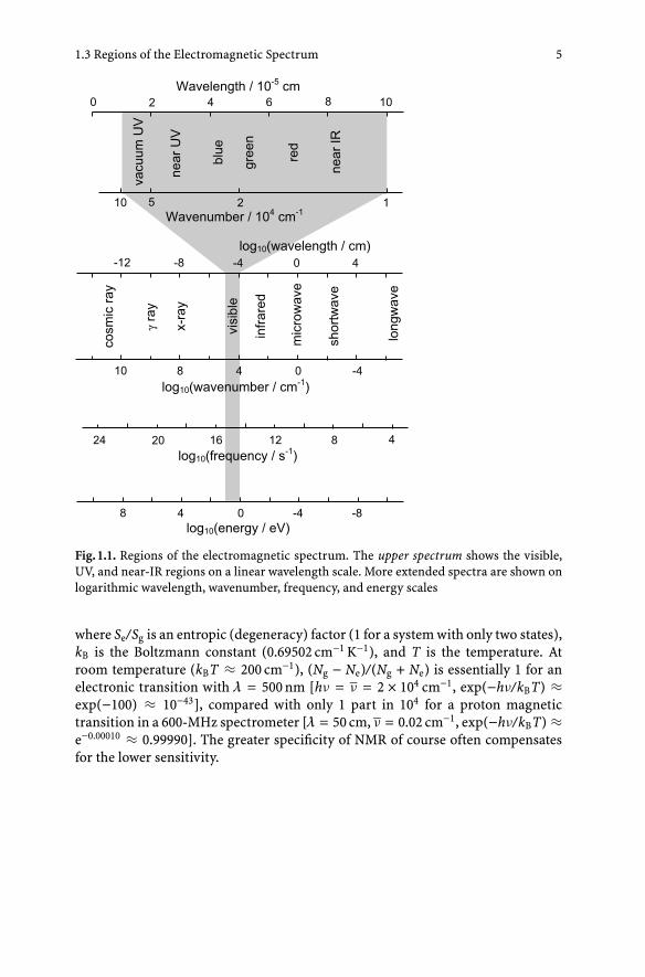
The regions of the electromagnetic spectrum that will be most pertinent to ourdiscussion involve wavelengths between 10−9 and 10−2 cm. Visible light fills onlythe small part of this range between 3 × 10−5 and 8 × 10−5 cm (Fig. 1.1). Transitionsof bonding electrons occur mainly in this region and the neighboring UV region;vibrational transitions occur in the IR. Rotational transitions are measurable in thefar-IR region in small molecules, but in macromolecules these transitions are toocongested to resolve. Radiation in the X-ray region can cause transitions in which1s or other core electrons are excited to atomic 3d or 4f shells or are dislodgedcompletely from a molecule. These transitions can report on the oxidation andcoordination states of metal atoms in metalloproteins.

The inherent sensitivity of absorption measurements in different regions of theelectromagnetic spectrum decreases with increasing wavelength because, in theidealized case of a molecule that absorbs and emits radiation at a single frequency,it depends on the difference between the populations of molecules in the groundand excited states. If the two populations are the same, radiation at the resonancefrequency will cause upward and downward transitions at the same rate, givinga net absorbance of zero. At thermal equilibrium, the fractional difference in thepopulations is given by

(Ng − Ne)

(Ng + Ne)=

[1 − (Se/Sg) exp(−ΔE/kBT)

]

[1 + (Se/Sg) exp(−ΔE/kBT)

] ≈ [1 − exp(−hν/kBT)][1 + exp(−hν/kBT)]

, (1.5)

1.3 Regions of the Electromagnetic Spectrum 5

Fig. 1.1. Regions of the electromagnetic spectrum. The upper spectrum shows the visible,UV, and near-IR regions on a linear wavelength scale. More extended spectra are shown onlogarithmic wavelength, wavenumber, frequency, and energy scales

where Se/Sg is an entropic (degeneracy) factor (1 for a system with only two states),kB is the Boltzmann constant (0.69502 cm−1 K−1), and T is the temperature. Atroom temperature (kBT ≈ 200 cm−1), (Ng − Ne)/(Ng + Ne) is essentially 1 for anelectronic transition with λ = 500 nm [hν = ν = 2 × 104 cm−1, exp(−hν/kBT) ≈exp(−100) ≈ 10−43], compared with only 1 part in 104 for a proton magnetictransition in a 600-MHz spectrometer [λ = 50 cm, ν = 0.02 cm−1, exp(−hν/kBT) ≈e−0.00010 ≈ 0.99990]. The greater specificity of NMR of course often compensatesfor the lower sensitivity.

6 1 Introduction

1.4Absorption Spectra of Proteins and Nucleic Acids

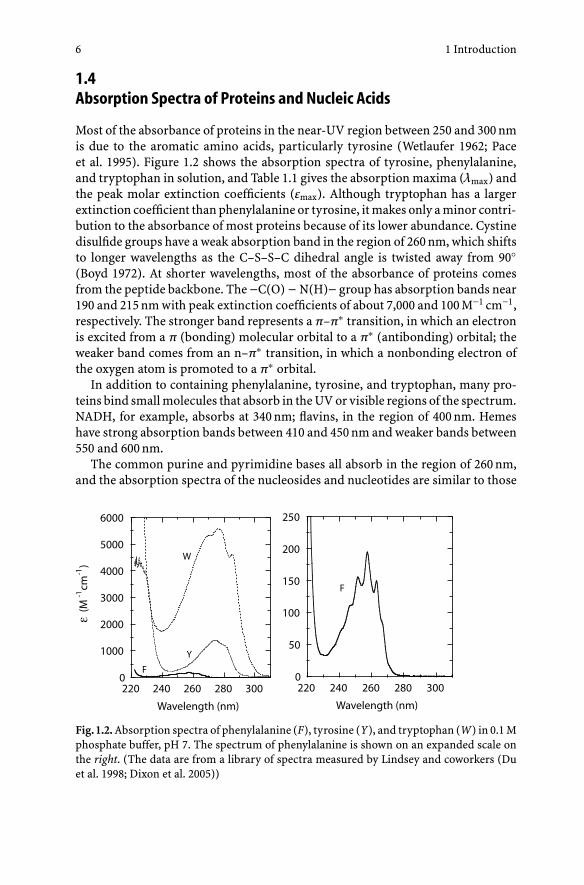
Most of the absorbance of proteins in the near-UV region between 250 and 300 nmis due to the aromatic amino acids, particularly tyrosine (Wetlaufer 1962; Paceet al. 1995). Figure 1.2 shows the absorption spectra of tyrosine, phenylalanine,and tryptophan in solution, and Table 1.1 gives the absorption maxima (λmax) andthe peak molar extinction coefficients (εmax). Although tryptophan has a largerextinction coefficient than phenylalanine or tyrosine, it makes only a minor contri-bution to the absorbance of most proteins because of its lower abundance. Cystinedisulfide groups have a weak absorption band in the region of 260 nm, which shiftsto longer wavelengths as the C–S–S–C dihedral angle is twisted away from 90◦(Boyd 1972). At shorter wavelengths, most of the absorbance of proteins comesfrom the peptide backbone. The −C(O) − N(H)− group has absorption bands near190 and 215 nm with peak extinction coefficients of about 7,000 and 100 M−1 cm−1,respectively. The stronger band represents a π–π∗ transition, in which an electronis excited from a π (bonding) molecular orbital to a π∗ (antibonding) orbital; theweaker band comes from an n–π∗ transition, in which a nonbonding electron ofthe oxygen atom is promoted to a π∗ orbital.

In addition to containing phenylalanine, tyrosine, and tryptophan, many pro-teins bind small molecules that absorb in the UV or visible regions of the spectrum.NADH, for example, absorbs at 340 nm; flavins, in the region of 400 nm. Hemeshave strong absorption bands between 410 and 450 nm and weaker bands between550 and 600 nm.

The common purine and pyrimidine bases all absorb in the region of 260 nm,and the absorption spectra of the nucleosides and nucleotides are similar to those

Fig. 1.2. Absorption spectra of phenylalanine (F), tyrosine (Y), and tryptophan (W) in 0.1 Mphosphate buffer, pH 7. The spectrum of phenylalanine is shown on an expanded scale onthe right. (The data are from a library of spectra measured by Lindsey and coworkers (Duet al. 1998; Dixon et al. 2005))

1.4 Absorption Spectra of Proteins and Nucleic Acids 7

Table 1.1. Absorption maxima and peak molar extinction coefficients of amino acids,purines, and pyrimidines in aqueous solution

Absorber λmax (nm)a εpeak (M−1 cm−1)a ε280 (M−1 cm−1)b

Tryptophan 278 5,580 5,500Tyrosine 274 1,405 1,490Cystine – – 125Phenylalanine 258 195

Adenine 261 13,400Guanine 273 13,150Uracil 258 8,200Thymine 264 7,900Cytosine 265 4,480a0.1 M phosphate buffer, pH 7.0. From Fasman (1976)bBest fit of values for 80 folded proteins in water. From Pace et al. (1995)

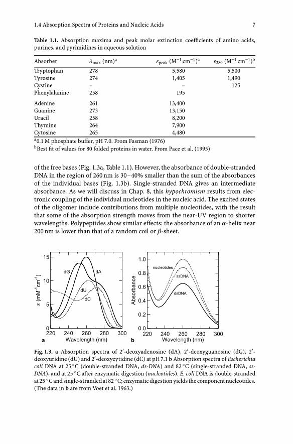
of the free bases (Fig. 1.3a, Table 1.1). However, the absorbance of double-strandedDNA in the region of 260 nm is 30–40% smaller than the sum of the absorbancesof the individual bases (Fig. 1.3b). Single-stranded DNA gives an intermediateabsorbance. As we will discuss in Chap. 8, this hypochromism results from elec-tronic coupling of the individual nucleotides in the nucleic acid. The excited statesof the oligomer include contributions from multiple nucleotides, with the resultthat some of the absorption strength moves from the near-UV region to shorterwavelengths. Polypeptides show similar effects: the absorbance of an α-helix near200 nm is lower than that of a random coil or β-sheet.

Fig. 1.3. a Absorption spectra of 2′-deoxyadenosine (dA), 2′-deoxyguanosine (dG), 2′-deoxyuridine (dU) and 2′-deoxycytidine (dC) at pH 7.1 b Absorption spectra of Escherichiacoli DNA at 25 ◦C (double-stranded DNA, ds-DNA) and 82 ◦C (single-stranded DNA, ss-DNA), and at 25 ◦C after enzymatic digestion (nucleotides). E. coli DNA is double-strandedat 25 ◦C and single-stranded at 82 ◦C; enzymatic digestion yields the component nucleotides.(The data in b are from Voet et al. 1963.)

8 1 Introduction

1.5Absorption Spectra of Mixtures

An important corollary of the Beer–Lambert law (Eq. (1.1)) is that the absorbanceof a mixture of noninteracting molecules is just the sum of the absorbances ofthe individual components. This means that the absorbance change resulting froma change in the concentration of one of the components is independent of theabsorbance due to the other components. In principle, we can determine theconcentrations of all the components by measuring the absorbance of the solutionat a set of wavelengths where the molar extinction coefficients of the componentsdiffer. The concentrations (Ci) are obtained by solving the simultaneous equations

ε1(λ1)C1 + ε2(λ1)C2 + ε3(λ1)C3 + · · · = Aλ1/lε1(λ2)C1 + ε2(λ2)C2 + ε3(λ2)C3 + · · · = Aλ2/l (1.6)

ε1(λ3)C1 + ε2(λ3)C2 + ε3(λ3)C3 + · · · = Aλ3/l· · · ,

where εi(λa) and Aλa are the molar extinction coefficient of component i and theabsorbance of the solution at wavelength λa, and l again is the optical path length.(A method for solving such a set of equations is given in Box 8.1.) The concentra-tions are completely determined when the number of measurement wavelengths isthe same as the number of components, as long as the extinction coefficients of thecomponents differ significantly at each wavelength. Measurements at additionalwavelengths can be used to increase the reliability of the results. The best way tocalculate the concentrations then probably is to use singular-value decomposition(Press et al. 1989).

Although two chemically distinct molecules usually have characteristically dif-ferent absorption spectra, their extinction coefficients may be identical at one ormore wavelengths. In the notation used above, εi(λa) and εj(λa) (the extinction co-efficients of components i and j at wavelength a) may be the same (Fig. 1.4a). Sucha wavelength is termed an isosbestic point. If we change the ratio of the concentra-tions Ci and Cj in a solution, the absorbance at the isosbestic points will remainconstant (Fig. 1.4b). If the solution contains a third component (k) we might haveεi(λb) = εk(λb) and εj(λc) = εk(λc) at two other wavelengths (b and c), but it wouldbe unlikely for all three components to have identical extinction coefficients atany wavelength. Thus, if we have a solution containing an unknown number ofcomponents and the absorption spectrum of the solution changes as a functionof a parameter such as pH, temperature, or time, the observation of an isosbesticpoint indicates that the absorbance changes probably reflect changes in the ratioof only two components. The reliability of this conclusion increases if there aretwo isosbestic points.

Protein concentrations often are estimated from the absorbance at 280 nm,where the only amino acids that absorb significantly are tryptophan, tyrosine, andcystine (Table 1.1). The molar extinction coefficient of a protein at this wavelengthis given by ε280 ≈ 5,500 × W + 1,490 × Y + 125 × CC M−1 cm−1, where W, Y, and CC

1.6 The Photoelectric Effect 9

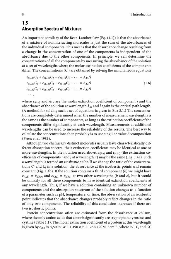
Fig. 1.4. Absorption spectra of two species that have the same extinction coefficient at 333 nm(a) and of mixtures of the same two components in molar ratios of 1:3, 1:1, and 3:1 (b). Notethat the total absorbance at the isosbestic point (333 nm) is constant

are the numbers of tryptophan, tyrosine, and cystine residues in the protein (Paceet al. 1995).

1.6The Photoelectric Effect

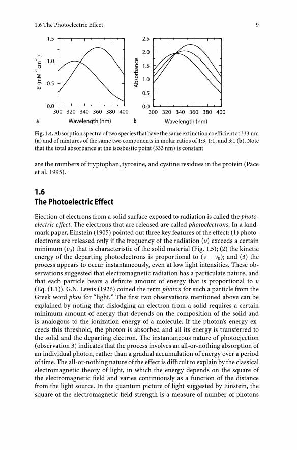
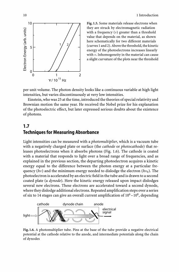
Ejection of electrons from a solid surface exposed to radiation is called the photo-electric effect. The electrons that are released are called photoelectrons. In a land-mark paper, Einstein (1905) pointed out three key features of the effect: (1) photo-electrons are released only if the frequency of the radiation (ν) exceeds a certainminimum (ν0) that is characteristic of the solid material (Fig. 1.5); (2) the kineticenergy of the departing photoelectrons is proportional to (ν − ν0); and (3) theprocess appears to occur instantaneously, even at low light intensities. These ob-servations suggested that electromagnetic radiation has a particulate nature, andthat each particle bears a definite amount of energy that is proportional to ν

(Eq. (1.1)). G.N. Lewis (1926) coined the term photon for such a particle from theGreek word phos for “light.” The first two observations mentioned above can beexplained by noting that dislodging an electron from a solid requires a certainminimum amount of energy that depends on the composition of the solid andis analogous to the ionization energy of a molecule. If the photon’s energy ex-ceeds this threshold, the photon is absorbed and all its energy is transferred tothe solid and the departing electron. The instantaneous nature of photoejection(observation 3) indicates that the process involves an all-or-nothing absorption ofan individual photon, rather than a gradual accumulation of energy over a periodof time. The all-or-nothing nature of the effect is difficult to explain by the classicalelectromagnetic theory of light, in which the energy depends on the square ofthe electromagnetic field and varies continuously as a function of the distancefrom the light source. In the quantum picture of light suggested by Einstein, thesquare of the electromagnetic field strength is a measure of number of photons

10 1 Introduction

Fig. 1.5. Some materials release electrons whenthey are struck by electromagnetic radiationwith a frequency (ν) greater than a thresholdvalue that depends on the material, as shownhere schematically for two different materials(curves 1 and 2). Above the threshold, the kineticenergy of the photoelectrons increases linearlywith ν. Inhomogeneity in the material can causea slight curvature of the plots near the threshold

per unit volume. The photon density looks like a continuous variable at high lightintensities, but varies discontinuously at very low intensities.

Einstein, who was 25 at the time, introduced the theories of special relativity andBrownian motion the same year. He received the Nobel prize for his explanationof the photoelectric effect, but later expressed serious doubts about the existenceof photons.

1.7Techniques for Measuring Absorbance

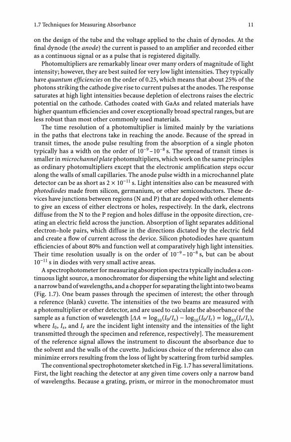
Light intensities can be measured with a photomultiplier, which is a vacuum tubewith a negatively charged plate or surface (the cathode or photocathode) that re-leases photoelectrons when it absorbs photons (Fig. 1.6). The cathode is coatedwith a material that responds to light over a broad range of frequencies, and asexplained in the previous section, the departing photoelectron acquires a kineticenergy equal to the difference between the photon energy at a particular fre-quency (hν) and the minimum energy needed to dislodge the electron (hν0). Thephotoelectron is accelerated by an electric field in the tube and is drawn to a secondcoated plate (a dynode). Here the kinetic energy released upon impact dislodgesseveral new electrons. These electrons are accelerated toward a second dynode,where they dislodge additional electrons. Repeated amplification steps over a seriesof six to 14 stages can give an overall current amplification of 106 –108, depending

Fig. 1.6. A photomultiplier tube. Pins at the base of the tube provide a negative electricalpotential at the cathode relative to the anode, and intermediate potentials along the chainof dynodes

1.7 Techniques for Measuring Absorbance 11

on the design of the tube and the voltage applied to the chain of dynodes. At thefinal dynode (the anode) the current is passed to an amplifier and recorded eitheras a continuous signal or as a pulse that is registered digitally.

Photomultipliers are remarkably linear over many orders of magnitude of lightintensity; however, they are best suited for very low light intensities. They typicallyhave quantum efficiencies on the order of 0.25, which means that about 25% of thephotons striking the cathode give rise to current pulses at the anodes. The responsesaturates at high light intensities because depletion of electrons raises the electricpotential on the cathode. Cathodes coated with GaAs and related materials havehigher quantum efficiencies and cover exceptionally broad spectral ranges, but areless robust than most other commonly used materials.

The time resolution of a photomultiplier is limited mainly by the variationsin the paths that electrons take in reaching the anode. Because of the spread intransit times, the anode pulse resulting from the absorption of a single photontypically has a width on the order of 10−9 –10−8 s. The spread of transit times issmaller in microchannel plate photomultipliers, which work on the same principlesas ordinary photomultipliers except that the electronic amplification steps occuralong the walls of small capillaries. The anode pulse width in a microchannel platedetector can be as short as 2 × 10−11 s. Light intensities also can be measured withphotodiodes made from silicon, germanium, or other semiconductors. These de-vices have junctions between regions (N and P) that are doped with other elementsto give an excess of either electrons or holes, respectively. In the dark, electronsdiffuse from the N to the P region and holes diffuse in the opposite direction, cre-ating an electric field across the junction. Absorption of light separates additionalelectron–hole pairs, which diffuse in the directions dictated by the electric fieldand create a flow of current across the device. Silicon photodiodes have quantumefficiencies of about 80% and function well at comparatively high light intensities.Their time resolution usually is on the order of 10−9 –10−8 s, but can be about10−11 s in diodes with very small active areas.

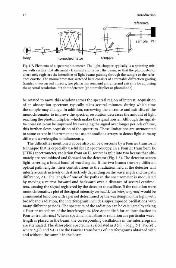
A spectrophotometer for measuring absorption spectra typically includes a con-tinuous light source, a monochromator for dispersing the white light and selectinga narrow band of wavelengths, and a chopper for separating the light into two beams(Fig. 1.7). One beam passes through the specimen of interest; the other througha reference (blank) cuvette. The intensities of the two beams are measured witha photomultiplier or other detector, and are used to calculate the absorbance of thesample as a function of wavelength [ΔA = log10(I0/Is) − log10(I0/Ir) = log10(Ir/Is),where I0, Is, and Ir are the incident light intensity and the intensities of the lighttransmitted through the specimen and reference, respectively]. The measurementof the reference signal allows the instrument to discount the absorbance due tothe solvent and the walls of the cuvette. Judicious choice of the reference also canminimize errors resulting from the loss of light by scattering from turbid samples.

The conventional spectrophotometer sketched in Fig. 1.7 has several limitations.First, the light reaching the detector at any given time covers only a narrow bandof wavelengths. Because a grating, prism, or mirror in the monochromator must

12 1 Introduction

Fig. 1.7. Elements of a spectrophotometer. The light chopper typically is a spinning mir-ror with sectors that alternately transmit and reflect the beam, so that the photodetectoralternately registers the intensities of light beams passing through the sample or the refer-ence cuvette. The monochromator sketched here consists of a rotatable diffraction grating(shaded), two curved mirrors, two planar mirrors, and entrance and exit slits for adjustingthe spectral resolution. PD photodetector (photomultiplier or photodiode)

be rotated to move this window across the spectral region of interest, acquisitionof an absorption spectrum typically takes several minutes, during which timethe sample may change. In addition, narrowing the entrance and exit slits of themonochromator to improve the spectral resolution decreases the amount of lightreaching the photomultiplier, which makes the signal noisier. Although the signal-to-noise ratio can be improved by averaging the signal over longer periods of time,this further slows acquisition of the spectrum. These limitations are surmountedto some extent in instruments that use photodiode arrays to detect light at manydifferent wavelengths simultaneously.

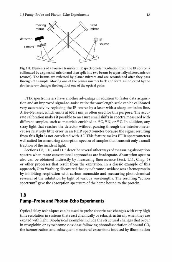
The difficulties mentioned above also can be overcome by a Fourier transformtechnique that is especially useful for IR spectroscopy. In a Fourier transform IR(FTIR) spectrometer, radiation from an IR source is split into two beams that ulti-mately are recombined and focused on the detector (Fig. 1.8). The detector senseslight covering a broad band of wavelengths. If the two beams traverse differentoptical path lengths, their contributions to the radiation field at the detector willinterfere constructively or destructively depending on the wavelength and the pathdifference, ΔL. The length of one of the paths in the spectrometer is modulatedby moving a mirror forward and backward over a distance of several centime-ters, causing the signal registered by the detector to oscillate. If the radiation weremonochromatic, a plot of the signal intensity versusΔL (an interferogram) would bea sinusoidal function with a period determined by the wavelength of the light; withbroadband radiation, the interferogram includes superimposed oscillations withmany different periods. The spectrum of the radiation can be calculated by takinga Fourier transform of the interferogram. (See Appendix 3 for an introduction toFourier transforms.) When a specimen that absorbs radiation at a particular wave-length is placed in the beam, the corresponding oscillations in the interferogramare attenuated. The absorption spectrum is calculated as A(ν) = log10[Sr(ν)/Ss(ν)],where Ss(ν) and Sr(ν) are the Fourier transforms of interferograms obtained withand without the sample in the beam.

1.8 Pump–Probe and Photon-Echo Experiments 13

Fig. 1.8. Elements of a Fourier transform IR spectrometer. Radiation from the IR source iscollimated by a spherical mirror and then split into two beams by a partially silvered mirror(center). The beams are reflected by planar mirrors and are recombined after they passthrough the sample. Moving one of the planar mirrors back and forth as indicated by thedouble arrow changes the length of one of the optical paths

FTIR spectrometers have another advantage in addition to faster data acquisi-tion and an improved signal-to-noise ratio: the wavelength scale can be calibratedvery accurately by replacing the IR source by a laser with a sharp emission line.A He–Ne laser, which emits at 632.8 nm, is often used for this purpose. The accu-rate calibration makes it possible to measure small shifts in spectra measured withdifferent samples, such as materials enriched in 13C, 15N, or 18O. In addition, anystray light that reaches the detector without passing through the interferometercauses relatively little error in an FTIR spectrometer because the signal resultingfrom this light is not correlated with ΔL. This feature makes FTIR spectrometerswell suited for measuring absorption spectra of samples that transmit only a smallfraction of the incident light.

Sections 1.8, 1.10, and 11.5 describe several other ways of measuring absorptionspectra when more conventional approaches are inadequate. Absorption spectraalso can be obtained indirectly by measuring fluorescence (Sect. 1.11, Chap. 5)or other processes that result from the excitation. In a classic example of thisapproach, Otto Warburg discovered that cytochrome c oxidase was a hemoproteinby inhibiting respiration with carbon monoxide and measuring photochemicalreversal of the inhibition by light of various wavelengths. The resulting “actionspectrum” gave the absorption spectrum of the heme bound to the protein.

1.8Pump–Probe and Photon-Echo Experiments

Optical delay techniques can be used to probe absorbance changes with very hightime resolution in systems that react chemically or relax structurally when they areexcited with light. Biophysical examples include the structural changes that occurin myoglobin or cytochrome c oxidase following photodissociation of bound CO,the isomerization and subsequent structural excursions induced by illumination

14 1 Introduction

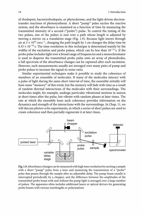
of rhodopsin, bacteriorhodopsin, or phytochrome, and the light-driven electron-transfer reactions of photosynthesis. A short “pump” pulse excites the reactivesystem, and the absorbance is examined as a function of time by measuring thetransmitted intensity of a second (“probe”) pulse. To control the timing of thetwo pulses, one of the pulses is sent over a path whose length is adjusted bymoving a mirror on a translation stage (Fig. 1.9). Because light moves throughair at 3 × 1010 cm s−1, changing the path length by 1 cm changes the delay time by0.33 × 10−10 s. The time resolution in this technique is determined mainly by thewidths of the excitation and probe pulses, which can be less than 10−14 s. If theprobe pulse includes light over a broad range of frequencies and a monochromatoris used to disperse the transmitted probe pulse onto an array of photodiodes,a full spectrum of the absorbance changes can be captured after each excitation.However, such measurements usually are averaged over many pairs of pump andprobe pulses to increase the signal-to-noise ratio.

Similar experimental techniques make it possible to study the coherence ofmembers of an ensemble of molecules. If many of the molecules interact witha pulse of light during the same short interval of time, the ensemble initially willhave some “memory” of this event, but the memory will fade with time as a resultof random thermal interactions of the molecules with their surroundings. Themolecules might, for example, undergo particular vibrational motions in unisonat short times after the pulse, but vibrate with random phases at later times. Therate at which the ensemble loses such coherence provides information on thedynamics and strength of the interactions with the surroundings. In Chap. 11, wewill discuss photon-echo experiments, in which a series of short pulses are used tocreate coherence and then partially regenerate it at later times.

Fig. 1.9. Absorbance changes can be measured with high time resolution by exciting a samplewith a short “pump” pulse from a laser and measuring the transmission of a “probe”pulse that passes through the sample after an adjustable delay. The pump beam usually isinterrupted periodically by a chopper, and the difference between the amplitudes of thetransmitted probe beam with and without the pump light is averaged over a large numberof pulses. The apparatus often includes additional lasers or optical devices for generatingprobe beams with various wavelengths or polarizations

1.9 Linear and Circular Dichroism 15

1.9Linear and Circular Dichroism

We mentioned earlier that absorption of light by a molecule requires that theoscillating electromagnetic field be oriented in a particular way relative to themolecular axes. The absorbance is proportional to cos2 θ, where θ is the anglebetween the electric field and the molecule’s transition dipole. Linear dichroism isthe dependence of absorption strength on the linear polarization of the light beamrelative to a macroscopic “laboratory” axis. Molecules in solution usually do notexhibit linear dichroism because the individual molecules are oriented randomlyrelative to the laboratory axes. However, proteins and other macromolecules oftencan be oriented by flow through a fine tube, or by compression or stretching ofsamples embedded in gels such as polyacrylamide or polyvinyl alcohol. Membranescan be oriented by magnetic fields or by drying in multiple layers on a glassslide. The linear dichroism of such samples can be measured with a conventionalspectrophotometer equipped with a polarizing filter that is oriented alternatelyparallel and perpendicular to the orientation axis of the sample.

Isotropic (disordered) samples often can be made to exhibit a transient lineardichroism (induced dichroism) by excitation with a polarized flash of light, becausethe flash selectively excites those molecules that happen to be oriented in a par-ticular way at the time of the flash. The decay kinetics of the induced dichroismprovides information on the rotational dynamics of the molecule. Such measure-ments are useful for exploring the disposition and rotational mobility of smallchromophores (light-absorbing molecules or groups) bound to macromoleculesor embedded in membranes, and for dissecting absorption spectra of complex sys-tems containing multiple interacting pigments. We will discuss linear dichroismfurther in Chap. 4.

A beam of light also can be circularly polarized, which means that the orien-tation of the electric field at a given position along the beam rotates with time.The rotation frequency is the same as the classical oscillation frequency of thefield (ν), but the direction of the rotation can be either clockwise or counterclock-wise from the perspective of an observer looking into the oncoming beam. Thesedirections correspond to left- and right-handed screws, and are called “left” and“right” circular polarization, respectively. Many natural materials exhibit differ-ences between their absorbance of left and right circularly polarized light. Thisis circular dichroism. The effect typically is small (about 1 part in 104), but canbe measured by using an electro-optic modulator to switch the measuring beamrapidly back and forth between right and left circular polarization. A phase- andfrequency-sensitive amplifier is used to extract the small oscillatory component ofthe light beam transmitted through the sample.

Because it represents the difference between two absorption strengths, circu-lar dichroism can be either positive or negative. It differs in this respect fromthe ordinary absorbance of a sample, which is always positive. Its magnitude isexpressed most directly by the difference between the molar extinction coeffi-

16 1 Introduction

cients for left and right circularly polarized light (Δε = εleft − εright in units ofM−1 cm−1); however, for historical reasons circular dichroism often is expressedin angular units (ellipticity or molar ellipticity), which relate to the elliptical po-larization that is generated when a beam of linearly polarized light is partiallyabsorbed.

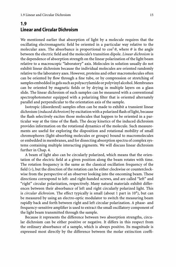
In order to exhibit circular dichroism, the absorbing molecule must be distin-guishable from its mirror image. Proteins and nucleic acids generally meet thiscriterion. As mentioned earlier in connection with hypochromism, their UV ab-sorption bands represent coupled transitions of multiple chromophores (peptidebonds or purine and pyrimidine bases), which are arranged stereospecifically withrespect to each other. The arrangement of the peptide bonds in a right-handedα-helix, for example, is distinguishable from that in a left-handed α-helix. Sucholigomers can have relatively strong circular dichroism even if the individual unitshave little or none (Tinoco 1961). Circular dichroism thus provides a convenientand sensitive way to probe secondary structure in proteins, nucleic acids, andmultimolecular complexes (Greenfield and Fasman 1969; Johnson and Tinoco1972; Brahms et al. 1977). Figure 1.10 shows typical circular dichroism spectra ofpolypeptides in α-helical and β conformations. The α-helix has a positive bandnear 195 nm and a characteristic pair of negative bands near 210 and 220 nm;the β-sheet has a weaker positive band near 200 nm and a solitary negative bandaround 215 nm. In Chap. 9, we will see that circular dichroism arises from interac-tions of the absorber with both the magnetic and the electric fields of the incidentradiation and we will discuss how its magnitude depends on the geometry of thesystem.

Fig. 1.10. Typical circular dichroism spectra of a polypeptide in α-helical and antiparallelβ-sheet conformations

1.10 Distortions of Absorption Spectra 17

1.10Distortions of Absorption Spectra by Light Scatteringor Nonuniform Distributions of the Absorbing Molecules

Absorption spectra of suspensions of cells, organelles, or large molecular com-plexes can be distorted severely by light scattering. Scattering results from inter-ference between optical rays that pass through or by the suspended particles, andit becomes increasingly important when the physical dimensions of the particlesapproach the wavelength of the light. Its hallmark is a baseline that departs fromzero outside the true absorption bands of the material and that rises with decreas-ing wavelength. Light that is scattered by more than a certain angle with respectto the incident beam misses the detector and registers as an apparent absorbance.The effect is greatest if the spectrophotometer has a long distance between thesample and the detector. There are several ways to minimize this distortion. One isto use an integrating sphere, a device designed to make the probability of reachingthe detector relatively independent of the angle at which light leaves the sample.This can be achieved by placing the specimen in a chamber with white walls andpositioning the detector behind a baffle so that light reaches the detector only afterbouncing off the walls many times (Fig. 1.11).

An integrating sphere also can be made by lining the walls with a large numberof photodiodes. In some cases light scattering can be decreased by fragmenting theoffending particles or by increasing the refractive index of the solvent by the addi-tion of a substance such as albumen. Mathematical corrections for scattering canbe made if the absorption spectrum is measured with the sample placed at severaldifferent distances from the detector (Latimer and Eubanks 1962; Naqvi et al. 1997).

Absorption spectra of turbid materials and even of specimens as dense asintact leaves or lobster shells also can be measured by photoacoustic spectroscopy.A photoacoustic spectrometer measures the heat that is dissipated when a sampleis excited by light and then decays nonradiatively back to the ground state. In

Fig. 1.11. An integrating sphere. The square in the middle represents a cuvette containinga turbid sample (S). Transmitted and scattered light reach the detector after many bouncesoff the white walls of the chamber. A baffle blocks the direct path to the detector. In onedesign (Kramer and Sacksteder 1998), the light passes through separate integrating spheresbefore and after the sample

18 1 Introduction

a typical design, release of heat causes a gas or liquid surrounding the sample toexpand and the expansion is detected by a microphone. Such measurements canbe used to study intermolecular energy transfer and volume changes that followthe absorption of light, in addition to the absorption itself (Ort and Parson 1978;Arata and Parson 1981; Braslavsky and Heibel 1992; Feitelson and Mauzerall 1996;Sun and Mauzerall 1998).

A different type of distortion occurs if the absorbing molecules are not disperseduniformly in the solution, but rather are sequestered in microscopic domains suchas cells or organelles (Duysens 1956; Latimer and Eubanks 1962; Pulles et al. 1976;Naqvi et al. 1997). Figure 1.12 illustrates the problem. Because the light intensitydecreases as a beam of light traverses a domain that contains absorbers, moleculesat the rear of the domain are screened by molecules toward the front and haveless opportunity to contribute to the total absorbance. If light beams passingthrough different regions of the sample encounter significantly different numbersof absorbers, the measured absorption band will be flattened compared with theband that would be observed for a uniform solution. Mathematical correctionsfor this effect can be applied if the size and shape of the microscopic domains isknown (Duysens 1956; Latimer and Eubanks 1962; Pulles et al. 1976; Naqvi et al.,1997). Alternatively, a comparison of the spectra before and after the absorbingmolecules are dispersed with detergents can be used to estimate the size of thedomains. However, the latter procedure assumes that dispersing the moleculesdoes not affect their intrinsic absorbance. In Chap. 8 we will show that molecularinteractions can make the spectroscopic properties of an oligomer intrinsicallyvery different from the properties of the individual subunits.

It is interesting to note in passing that frogs, octopi, and some other animalsuse the spectral flattening effect to change their appearance. They appear darkwhen pigmented cells in their skin spread out to cover the surface more or lessuniformly, and pale when the cells clump together.

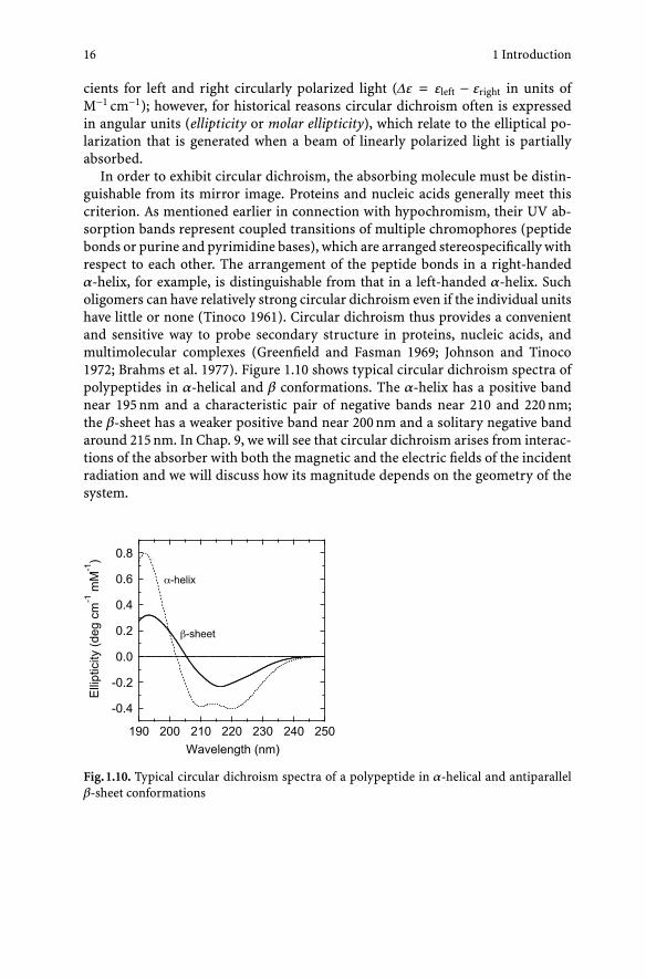
Fig. 1.12. The absorbance of a macroscopic sample depends on how the absorbing materialsare distributed. The boxes represent small volume elements; the shaded objects are absorbingmolecules. The overall concentration of absorbers is 0.5 per unit volume in both A and B.If the light intensity incident on a volume element is I0, the intensity transmitted by theelement can be written I1 = κI0, where 0 < κ < 1 if the element contains an absorberand κ = 1 if it does not. In the arrangement shown in A, light beams that pass through thespecimen in different places encounter the same number of absorbers. The light transmittedper unit area is I1 = κI0. In B, the two beams encounter different numbers of absorbers.Here the light transmitted per unit area is (I2 + I0)/2 = (κ2I0 + I0)/2. The difference (B − A)is (κ2I0 + I0 − 2κI0)/2 = I0(κ − 1)2/2, which is greater than zero

1.11 Fluorescence 19

Deviations from Beer’s law also can arise from a concentration-dependent equi-librium between different chemical species, or from changes in the refractive indexof the solution with concentration. Instrumental nonlinearities or noise may besignificant if the concentration of the absorber is too high or too low.

1.11Fluorescence

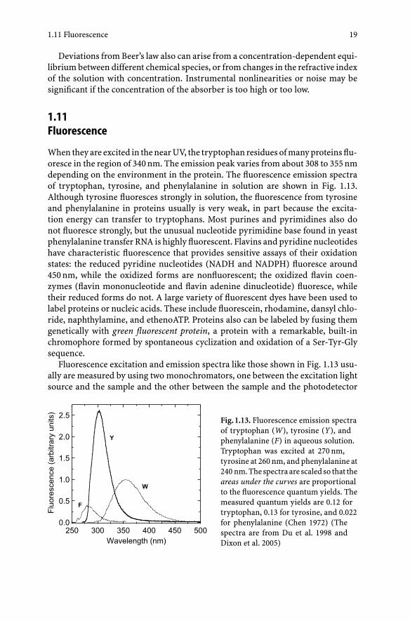
When they are excited in the near UV, the tryptophan residues of many proteins flu-oresce in the region of 340 nm. The emission peak varies from about 308 to 355 nmdepending on the environment in the protein. The fluorescence emission spectraof tryptophan, tyrosine, and phenylalanine in solution are shown in Fig. 1.13.Although tyrosine fluoresces strongly in solution, the fluorescence from tyrosineand phenylalanine in proteins usually is very weak, in part because the excita-tion energy can transfer to tryptophans. Most purines and pyrimidines also donot fluoresce strongly, but the unusual nucleotide pyrimidine base found in yeastphenylalanine transfer RNA is highly fluorescent. Flavins and pyridine nucleotideshave characteristic fluorescence that provides sensitive assays of their oxidationstates: the reduced pyridine nucleotides (NADH and NADPH) fluoresce around450 nm, while the oxidized forms are nonfluorescent; the oxidized flavin coen-zymes (flavin mononucleotide and flavin adenine dinucleotide) fluoresce, whiletheir reduced forms do not. A large variety of fluorescent dyes have been used tolabel proteins or nucleic acids. These include fluorescein, rhodamine, dansyl chlo-ride, naphthylamine, and ethenoATP. Proteins also can be labeled by fusing themgenetically with green fluorescent protein, a protein with a remarkable, built-inchromophore formed by spontaneous cyclization and oxidation of a Ser-Tyr-Glysequence.

Fluorescence excitation and emission spectra like those shown in Fig. 1.13 usu-ally are measured by using two monochromators, one between the excitation lightsource and the sample and the other between the sample and the photodetector

Fig. 1.13. Fluorescence emission spectraof tryptophan (W), tyrosine (Y), andphenylalanine (F) in aqueous solution.Tryptophan was excited at 270 nm,tyrosine at 260 nm, and phenylalanine at240 nm. The spectra are scaled so that theareas under the curves are proportionalto the fluorescence quantum yields. Themeasured quantum yields are 0.12 fortryptophan, 0.13 for tyrosine, and 0.022for phenylalanine (Chen 1972) (Thespectra are from Du et al. 1998 andDixon et al. 2005)

20 1 Introduction

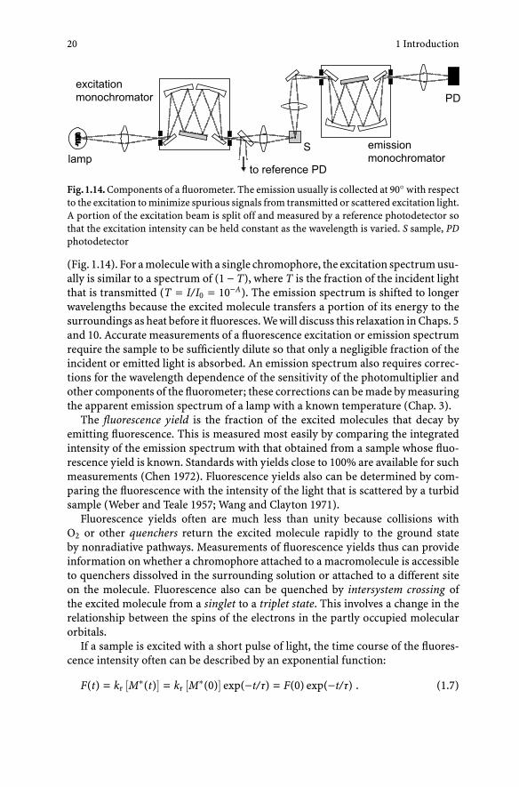
Fig. 1.14. Components of a fluorometer. The emission usually is collected at 90◦ with respectto the excitation to minimize spurious signals from transmitted or scattered excitation light.A portion of the excitation beam is split off and measured by a reference photodetector sothat the excitation intensity can be held constant as the wavelength is varied. S sample, PDphotodetector

(Fig. 1.14). For a molecule with a single chromophore, the excitation spectrum usu-ally is similar to a spectrum of (1 − T), where T is the fraction of the incident lightthat is transmitted (T = I/I0 = 10−A). The emission spectrum is shifted to longerwavelengths because the excited molecule transfers a portion of its energy to thesurroundings as heat before it fluoresces. We will discuss this relaxation in Chaps. 5and 10. Accurate measurements of a fluorescence excitation or emission spectrumrequire the sample to be sufficiently dilute so that only a negligible fraction of theincident or emitted light is absorbed. An emission spectrum also requires correc-tions for the wavelength dependence of the sensitivity of the photomultiplier andother components of the fluorometer; these corrections can be made by measuringthe apparent emission spectrum of a lamp with a known temperature (Chap. 3).

The fluorescence yield is the fraction of the excited molecules that decay byemitting fluorescence. This is measured most easily by comparing the integratedintensity of the emission spectrum with that obtained from a sample whose fluo-rescence yield is known. Standards with yields close to 100% are available for suchmeasurements (Chen 1972). Fluorescence yields also can be determined by com-paring the fluorescence with the intensity of the light that is scattered by a turbidsample (Weber and Teale 1957; Wang and Clayton 1971).

Fluorescence yields often are much less than unity because collisions withO2 or other quenchers return the excited molecule rapidly to the ground stateby nonradiative pathways. Measurements of fluorescence yields thus can provideinformation on whether a chromophore attached to a macromolecule is accessibleto quenchers dissolved in the surrounding solution or attached to a different siteon the molecule. Fluorescence also can be quenched by intersystem crossing ofthe excited molecule from a singlet to a triplet state. This involves a change in therelationship between the spins of the electrons in the partly occupied molecularorbitals.

If a sample is excited with a short pulse of light, the time course of the fluores-cence intensity often can be described by an exponential function:

F(t) = kr [M∗(t)] = kr [M∗(0)] exp(−t/τ) = F(0) exp(−t/τ) . (1.7)