IMPROVEMENTS IN FEA OF COMPOSITE OVERWRAPPED PRESSURE VESSELS

Rick P. Willardson eServ, a Perot Systems Company

2300 W. Plano Parkway Plano, TX 75075

David L. Gray Dassault Systemes Simulia Corp.

190 Civic Circle, Suite 210 Lewisville, TX 75067

Thomas K. DeLay NASA – Marshall Space Flight Center

Huntsville, AL 35812

ABSTRACT

Finite element analysis (FEA) of a composite overwrapped pressure vessel (COPV) has traditionally been a tedious and time consuming task. FEA is often omitted in the development of many vessels in favor of a “build and burst” philosophy based only on preliminary design with netting analysis. This is particularly true for small vessels or vessels that are not weight critical. The primary difficulty in FEA of a COPV is the creation of the model geometry on the sub-ply level. This paper discusses employing a commercially available tool to drastically reduce the time required to build a COPV FEA model. This method produces higher fidelity models in only slightly more time. Analysis results are presented along with comparisons to burst test data. Additionally the application that inspired this tool’s development is discussed.

1. INTRODUCTION

COPV’s have been in use for decades and are currently used in a variety of applications from giant solid rocket motor cases to tiny paint-ball gun pressure reservoirs. They are found most frequently in applications where component weight is critical. In these applications, COPV’s have obvious advantages over homogenous metallic pressure vessels.

This paper offers background on some of the issues involved with COPV design and analysis. It then compares traditional COPV design and analysis (netting analysis & manual FEA) to COPV design and analysis employing an automated FEA tool known as the Wound Composite Modeler (WCM) for ABAQUS. It also presents the results of a COPV design for a high pressure gas storage vessel using WCM. The target audience for this paper is individuals who are generally familiar with COPV design, analysis and fabrication. Not all terms, theories, techniques and methods are fully explained. More complete explanations are available in the references.

2. ACKNOWLEDGMENTS

This work would not have been possible without the unique cooperative efforts of the authors. Mr. DeLay provided the application parameters for the high pressure gas storage vessel; as well as fabrication and burst testing of the COPV with the accompanying data. Mr. Gray supplied a license of WCM for ABAQUS (along with its initial and continuing development). Mr. Willardson performed the design and analysis of the COPV.

3. BACKGROUND

Despite their wide-spread use, the development of many COPV designs is still rather primitive. Often only limited analysis is performed to obtain an initial design, and then the design is refined through a number of “build and burst” iterations. In this method, appropriate application of heuristic techniques (rules of thumb) and the experience of the designer play a large role in how many iterations are necessary to obtain a final design. For many applications, this method is perfectly adequate.

However for some applications, the cost in material and resources to fabricate multiple test articles is extremely prohibitive (large-scale rocket motor cases; large-scale liquid propellant tanks; or thick-walled, high pressure vessels, Figure 1). For these high value articles, FEA is often employed in an attempt to reduce the number of iterations required. If done manually, this process can be tedious and very time consuming. It commits fewer resources but requires substantial schedule commitment; which may be just as prohibitive to the product development process. Because of this, the FEA process does not lend itself to multiple iterations and effectively becomes more of a design confirmation effort rather than a design iteration effort.

Figure 1: Large Oxidizer Tank for a Launch Vehicle

For other applications the rules-of-thumb don’t completely apply. Traditionally, the rules are most applicable to certain dome shapes (geodesic) and even with these shapes the rules are not universally applicable. In fact; it has been the authors’ experience that these rules tend to break-down with vessels that have cylinder-to-opening diameter ratios greater than 5.75 or with vessels that are very thin-walled, diameter-to-thickness ratio greater than 50. Generally the more similar an application is to a rocket motor case, the better the rules will apply; because most of these rules were derived from rocket motor development experience [1].

Furthermore, traditional design and analysis tools have been somewhat out-paced by manufacturing tools. Computer-controlled filament winding machines and their associated software offer significant design flexibility and are readily available. With only modest effort, they can wind any pattern angle that the tool surface friction will maintain. They can also effectively vary ply thickness by varying the programmed band advanced. Many of the software packages can also output wind angles and thickness for use by FEA programs. However, most of these provide only shell element data, which for most COPV’s is an inappropriate use of FEA. Solid elements are much more appropriate for thick-walled pressure vessels and for large displacement geometrically nonlinear structures.

Thus for a more general COPV application that could take advantage of the latest manufacturing tools; a leaner, more accurate design and analysis process was necessary. Nowhere was this more obvious than at a start-up private launch vehicle company in the late 90’s. This company was developing a launch vehicle with a pressure-fed engine system. This engine system included three different types of COPV’s; relatively low-pressure fuel and oxidizer tanks and high-pressure gas storage vessels (see Figure 2).

Figure 2: Pressure-fed Rocket Engine System with COPV's for Oxidizer (center top), Fuel (center left-right) & Pressurization (extreme left-right) Tanks and Thrust Chamber (center)

All of these COPV’s needed to be very weight efficient for maximum vehicle performance. All of the issues discussed above were encountered in the development of these COPV’s. Nearly every vessel could be classified as a high value article with hundreds of kilograms of material and hundreds of man-hours invested in almost every one. The vessels were very large ranging from 1.5-meters to 6.2-meters in diameter. These large diameters resulted in dome contours and wall thickness that pushed the envelope of traditional COPV design. To further complicate the matter, the vessels were constructed on inflatable plastic liners that also served as “fly-away” tooling. Although never fully realized during this launch vehicle endeavor; this challenging environment was the genesis for the WCM tool.

4. TRADITIONAL COPV DESIGN AND ANALYSIS

4.1 Netting Analysis This closed form derivation is so named because of its primary assumptions. These assumptions assume that the overwrap acts like a “net” for the pressure load on the vessel. The first assumption is to ignore the contribution of the resin to the strength of the composite. All loads are assumed to be taken by the fibers only. The second assumption is that only a single helical wind angle takes the axial load on the vessel. These assumptions are inserted into the equations for stresses in the cylinder wall of a closed end vessel [2]. Below are the resulting equations for required helical and hoop fiber thickness

22 cosb cyl

helicaltlf

P Rt

σ θ=

[1]

2(2 tan )2b cyl

tlhoopf

P Rt θ

σ= −

[2]

Where Pb is the design burst pressure, Rcyl is the radius of the cylindrical section, σf is the ultimate tensile stress of the fiber (including any desired statistical or environmental reduction) and θtl is the helical angle at the dome tangent line. A more complete treatment of this derivation is given in reference [1]. These equations only size the cylinder of the vessel for pressure loads. They do not account for stresses in the domes or any other type of load on the vessel (bending or axial compression for instance).

To address stresses in the dome an empirical factor known as the stress ratio is employed. The stress ratio is defined as the stress in the helical plies divided by the stress in the hoop plies. These stresses are determined by solving for the stress term in equations 1 & 2, after determining an initial hoop and helical thickness. A stress ratio of 0.6 is typical for many vessels (particularly those with geodesic dome contours). The lower the stress ratio the more likely a vessel will fail in the hoop direction in the cylinder section (and vice versa for high stress ratios and dome failures). Employing smaller stress ratios effectively adds additional material to the dome of the vessel to compensate for the unknown stresses in that region. This method is inherently inexact and cannot account for several factors that complicate the stresses in the dome region, such as actual dome shape and the severe hoop stiffness discontinuity just past the cylinder-dome tangent.

The shape of a pressure vessel dome directly affects the stress in the dome as can be seen from the equations in reference [3]. The meridional stress varies directly with the hoop radius. The hoop stress varies inversely with the meridional radius. In other words, the more flat the dome is at any point the higher the hoop stress. For COPV’s, a method has been derived to shape the dome optimally for the composite overwrap. This method is an iterative calculation that changes the meridional dome radius to maintain the principal stress (vector combination of hoop and meridional stress) in the same direction as the wound fiber [1]. The resulting shape is called the geodesic or iso-tensiod dome. This shape is more optimal than ellipsoidal or spherical shapes for COPV’s; because it causes the stress to be aligned with the strongest direction of the composite.

Netting analysis and geodesic calculations despite their short-comings are still very useful techniques, especially for preliminary design. However as described in the background section above, many applications required more complete design and analysis methods.

4.2 Manual FEA When a better understanding of dome stresses is required, FEA can be employed. FEA can correct many of the short-comings of netting analysis. It can include multiple geometries; model the discontinuity at the cylinder-dome tangent; include the contribution of the resin to the composite; include multiple wind angles and determine stresses and strains in the dome region. However, the correct type of FEA model must be used depending on the loading scenario that is of interest (axisymetric continuum, 3D-shells or 3D-solids). If pressure is the primary load of interest then the FEA model is usually done with axisymetric elements.

As with all FEA, your results are only as good as your inputs; and many of the inputs required to analyze a COPV are not easy to obtain. The most difficult inputs to deal with can be separated into two general categories: 1) geometry and 2) materials.

The COPV geometry is not particularly difficult to obtain. However, turning this geometry into a useful FEA model can be challenging; and once an acceptable FEA model is constructed, making significant changes to it usually requires starting completely over.

One issue with the geometry is determining at what level to define the geometry. Does every ply need to be modeled or can they be grouped? If every ply needs to be modeled, the definition of this geometry can be tedious; and this small geometry can cause difficulty obtaining an acceptable FE mesh on the part. Usually three elements are preferred through the thickness of a ply. To adhere to this guideline; either the elements of the mesh will be extremely distorted or the number of elements required for the mesh will expand exponentially. If the COPV is very large, the number of elements can become prohibitive by increasing the resources and time required to solve the model.

Another issue with the geometry is determining how to account for the thickness build-up near the port of a COPV. There are simple equations that can be utilized, and as stated earlier, many of the filament winding software packages can assist with this task. However, these tools usually don’t define the actual termination of the helical ply and this geometry is left to the analyst to determine.

Perhaps the most difficult FEA input is the material property assignments, particularly for those elements in the dome region. The constantly changing angle of the fibers running down the dome is what makes this task challenging. Material orientations must either be assigned to acceptable discrete regions (for instance, every 5° of angle change) or to every single element. Appropriate material properties must then be computed for these regions. Additionally, these material properties must be compatible with the model geometry type and element type selected for the FEA model. For axisymetric continuum models, orthotropic properties (or orthotropic properties calculated from engineering constants) are usually used.

Some of these tasks can be easily automated; some are more difficult to automate. A few proprietary scripts exist at some COPV manufactures that semi-automate the process of constructing an FEA model. Obviously these scripts are not available to the general COPV community and are not regularly maintained and updated with the latest features (like most internal proprietary codes).

5. COPV DESIGN AND ANALYSIS WITH WOUND COMPOSITE MODELER (WCM) FOR ABAQUS

WCM for ABAQUS is one of the few commercially available codes that automates the entire process of constructing a COPV FEA model. The WCM code is integrated inside the ABAQUS/CAE pre-processor as a plug-in module. A complete description of how to construct COPV models with WCM is beyond the scope of this paper. This information is available in the WCM user’s manual [4]. This section will give a brief overview of the process used to construct the model of a high-pressure gas storage vessel that is used as a real-world example for this paper.

The software and documentation are publicly available from the Simulia website [5]. To successfully execute the code the proper licenses must be in place. The software setup is simple. Once the zip file is downloaded and extracted. Simply copy the WoundComposites folder into the appropriate abaqus_plugins directory and launch ABAQUS/CAE.

WCM is accessed from the plug-ins menu option. The tank manager dialog box is the main graphical user interface (GUI) for the WCM. The tank manager has options to create multiple domes and assign them to a complete vessel (see Figure 3). This option allows modeling of COPV’s with different polar openings on each end of the vessel. The example vessel has identical polar openings on each end, so only half of the vessel was modeled.

To create a dome in the tank manager, several parameters must be defined. These parameters are located in the wound composite dome window that is accessed by either the “create” or “edit” buttons in the tank manager window.

For the example vessel the dome and cylinder geometries were assigned first. A cylinder length of 228.6-mm (9-in) was used to model a complete half of the vessel. The dome geometry of the spin-formed liner was elliptical with a vessel radius of 279.7-mm (11.012-in) and a minor axis radius of ≈192-mm (7.6-in). The dome also had a 25.4-mm (1-in) radius to its 59.7-mm (2.35-in) diameter port opening. The dome was actually defined using the user-defined points option to account for this large radius (see Figure 4). Care should be taken when using the user-defined

or the from-part-instance options to define the dome geometry. Using a large number of points in the table or a finely-meshed part can significantly increase model regeneration time. This is because all the points in the original curve will be propagated as additional wound geometry is created.

Figure 3: Screen of Tank Manager Window

Next, the overwrap parameters were defined (see Figure 5). The winding layout layer termination was set to move to the transition point of the polar opening build-up. A generic epoxy material was used for the void material definition. The winding layout layers were defined using an initial netting analysis as a starting point. The material for all layers was defined as a T1000 carbon fiber composite. Repeated layers were grouped and given a total thickness to simplify the model regeneration. Helical layers are assumed to be two plies at +/- the wind angle defined in the table, so layer thicknesses need to be defined accordingly. Helical layers with no friction compensation were used for this vessel. With friction compensation, the wind angle and the radial opening can each be specified. Without friction compensation, only the wind angle can be specified. Approximately half of the helical layers go all the way down the dome to the polar opening; their radial terminations stagger back at the transition point of the previous layer. The helical layers are assigned a band width factor that represents the degree of band condensing (and resulting thickness build-up) of the material as it is wound on to the dome. This is just one of the many WCM features that incorporate manufacturing information into the

FEA. The remaining helical layers are stepped back up the dome in strategic locations. The shape of the helical end terminations were all set to “Spline, 1.0, 1.5, 0.5”. Hoop layers are assigned a height with the cylinder-dome tangent being the origin in this case. The first hoop layer was set 19-mm (0.75-in) forward of the tangent and the subsequent hoop layers were staggered back over ≈50.8-mm (2.0-in). The hoop layer end termination shapes were all set to “No Void, 3.0, 0.5”.

Figure 4: Dome Geometry Creation Screen Shot

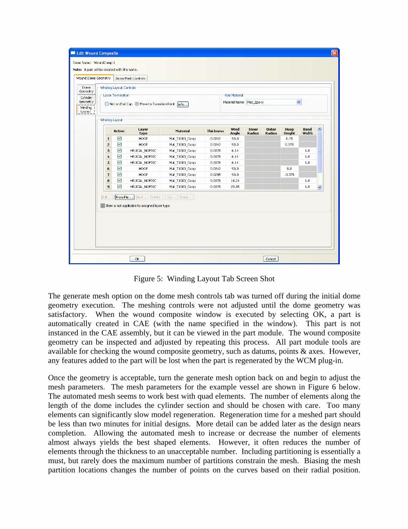
Figure 5: Winding Layout Tab Screen Shot

The generate mesh option on the dome mesh controls tab was turned off during the initial dome geometry execution. The meshing controls were not adjusted until the dome geometry was satisfactory. When the wound composite window is executed by selecting OK, a part is automatically created in CAE (with the name specified in the window). This part is not instanced in the CAE assembly, but it can be viewed in the part module. The wound composite geometry can be inspected and adjusted by repeating this process. All part module tools are available for checking the wound composite geometry, such as datums, points & axes. However, any features added to the part will be lost when the part is regenerated by the WCM plug-in.

Once the geometry is acceptable, turn the generate mesh option back on and begin to adjust the mesh parameters. The mesh parameters for the example vessel are shown in Figure 6 below. The automated mesh seems to work best with quad elements. The number of elements along the length of the dome includes the cylinder section and should be chosen with care. Too many elements can significantly slow model regeneration. Regeneration time for a meshed part should be less than two minutes for initial designs. More detail can be added later as the design nears completion. Allowing the automated mesh to increase or decrease the number of elements almost always yields the best shaped elements. However, it often reduces the number of elements through the thickness to an unacceptable number. Including partitioning is essentially a must, but rarely does the maximum number of partitions constrain the mesh. Biasing the mesh partition locations changes the number of points on the curves based on their radial position.

Adjusting this parameter and the number of elements along the dome can help reduce the number of skewed elements. The mesh can be viewed and inspected in the part specific section of the mesh module. The mesh can also be adjusted with traditional tools in the mesh module. However, on the example vessel this never improved the meshing results.

Figure 6: Dome Meshing Controls Screen Shot

Once the geometry and mesh are suitable, the parameters on the other tabs of the tank manager can be set (see Figure 7). For the example vessel the geometry space was axisymetric, continuum and the section assignment parameters are static with CAX4RH elements. In the model generation parameters, the thermal loads and pressure loads are turned off. Thermal loads were not analyzed for the example vessel and the pressure load is defined later on the liner in CAE. The symmetric boundary conditions are generated for the example model. The number of elements along the length is set to the same value as that for the dome part.

The material and section property generation, as well as generation of the UVARM subroutine, can be time consuming and are best done after satisfactory generation of the meshed model. This information can be generated at a later time with out regenerating the geometry and mesh by using the “regenerate properties” button (see Figure 7). Reference [6] contains information on the specifics of how the material properties are generated and how fiber directional data is extracted with the UVARM subroutine. To run the UVARM user-defined subroutine ABAQUS must be setup with a specific Fortran compiler and executed in the compiler environment.

Figure 7: Tank Manager - Model Generation Screen Shot

When the tank manager is executed by selecting OK, another part is automatically created in CAE (with the name specified in the tank manager window). This part is instanced in the CAE assembly and can be operated on in the interaction and loads module. For the example vessel, the aluminum liner is also instanced into the assembly and it is tied to the overwrap part with a TIE constraint in the interaction module. A closeout plate is also instanced into the assembly and tied to the liner in similar manner. The pressure is applied to the inside surface of the liner and closeout plate. The symmetric boundary condition is also applied to the liner. Once this is complete, the material properties and the UVARM subroutine are generated back in the tank manager window. At this point the model is ready to run. This highly detailed model can be created in a matter of a few hours.

This is just a limited overview of the capabilities of WCM. It has many other valuable features that have not been discussed here; such as the ability to include non-linear material shear plies, dome-only reinforcement or doilies, skirt attachments through additional modeling in CAE or other load cases besides simple internal pressure.

6. RESULTS

Figure 8 shows the final geometry of the example COPV. This model is the result of 9-iterations. The first 3-iterations took longer than expected (≈40-hrs) because the learning curve on this particular problem was steeper than expected. This was primarily due to the elliptical dome geometry. This geometry resulted in large stresses around the polar opening and at the cylinder to dome transition. It also caused a very unusual deflected shape which was coupled with the large stresses. The final 6-iterations were done in ≈12-hrs. Adding additional helical layers reduced the polar opening stresses and optimizing the deflected shape by changing the location of the higher angle helical layers lowered the stresses in the transition region. Figure 9 shows deflection plots for each iteration.

Figure 10 shows the strain in the fiber direction (UVARM2) for a pressure of 58.02-MPa (8415-psi). The gray areas are above the strain allowable used for the T1000 composite of 17986-µs. The FEA predicts the burst pressure at 57.56-MPa (8348-psi) in the first hoop ply of the cylinder section. The stress ratio (measured in the cylinder section) is 0.43.

Figure 11 shows a close-up view of the polar region fiber strains. They are just barely below the allowable. Figure 12 shows the equivalent plastic strain in the aluminum liner. All areas are under the 5.5% fracture strain used for 6061-T6.

The example vessel was fabricated according to the information in Figure 8. The wind angle on the first 9 helical patterns was either 9° or 11.5°. Two different patterns were alternated in a shingled manner to maximize coverage near the polar opening. The remaining 9 helical patterns were divided evenly among the three angles shown in the figure. Figure 13 shows the example vessel during fabrication. The final weight of the example vessel was 44.0-kg (97.0-lbs). Subtracting the measured liner weight gives a composite overwrap weight of 23.5-kg (51.9-lbs). The as-built thickness of the composite overwrap was 11.05-mm (0.435-in) measured in the cylinder section of the vessel. Three strain gages were placed on the vessel to gather data during burst testing. The gages were placed approximately as shown in Figure 8. This data is shown and compared to the FEA results in Figures 14-16. The example vessel burst at 53.17-MPa (7712-psi). The failure initiated in the vessel’s cylinder section as can be seen in Figure 17.

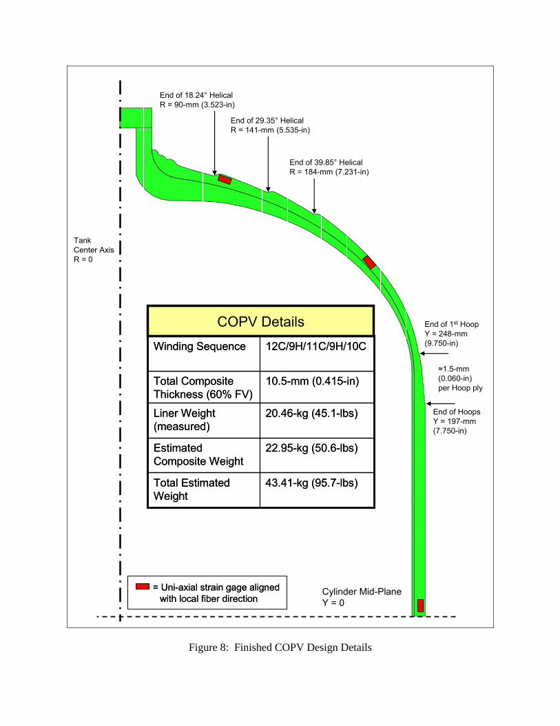
Cylinder Mid-PlaneY = 0

End of 1st HoopY = 248-mm (9.750-in)

End of HoopsY = 197-mm (7.750-in)

≈1.5-mm (0.060-in) per Hoop ply

End of 39.85° HelicalR = 184-mm (7.231-in)

Tank Center AxisR = 0

End of 29.35° HelicalR = 141-mm (5.535-in)

End of 18.24° HelicalR = 90-mm (3.523-in)

= Uni-axial strain gage aligned with local fiber direction

= Uni-axial strain gage aligned with local fiber direction

20.46-kg (45.1-lbs)Liner Weight (measured)

22.95-kg (50.6-lbs)Estimated Composite Weight

43.41-kg (95.7-lbs)Total Estimated Weight

10.5-mm (0.415-in)Total Composite Thickness (60% FV)

12C/9H/11C/9H/10CWinding Sequence

20.46-kg (45.1-lbs)Liner Weight (measured)

22.95-kg (50.6-lbs)Estimated Composite Weight

43.41-kg (95.7-lbs)Total Estimated Weight

10.5-mm (0.415-in)Total Composite Thickness (60% FV)

12C/9H/11C/9H/10CWinding Sequence

COPV Details

Figure 8: Finished COPV Design Details

0

0.05

0.1

0.15

0.2

0.25

0.3

0 5 10 15 20 25 30

Arc Length (mm)

Def

lect

ion

(mm

)

Design #1Design #2Design #3Design #4Design #5Design #6Design #7Design #8Design #9

7.62

6.35

5.08

3.81

2.54

1.27

127 254 381 508 762635

Figure 9: Deflection vs. Dome Location for Design Iterations (0 is cylinder mid-plane).

Max Strain = 18128-µs

008.011812817986.. −=−=SM

Figure 10: Fiber Direction Strain on Un-deformed Shape and on 10X Deformed Shape

Figure 11: Fiber Direction Strain in Polar Region

Figure 12: Equivalent Plastic Strain on Aluminum Liner

Figure 13: Vessel during Winding of First 39.85° Helical Pattern

0

1000

2000

3000

4000

5000

6000

7000

8000

9000

0 5000 10000 15000 20000 25000

Microstrain (µs)

Pre

ssur

e (M

Pa)

Original FEATest DataAdjusted FEA

62.05

34.47

55.16

48.26

41.37

27.58

20.68

13.79

6.89

Figure 14: Mid-Cylinder Hoop Strain Gage Data with Original and Adjusted FEA Results

0

1000

2000

3000

4000

5000

6000

7000

8000

9000

0 2000 4000 6000 8000 10000 12000 14000

Microstrain (µs)

Pres

sure

(MPa

)

Adjusted FEATest Data

62.05

34.47

55.16

48.26

41.37

27.58

20.68

13.79

6.89

Figure 15: Polar Opening Strain Gage Data (on 18.24° Helical) with Adjusted FEA Results

0

1000

2000

3000

4000

5000

6000

7000

8000

9000

-500 1500 3500 5500 7500 9500

Microstrain (µs)

Pres

sure

(MPa

)

Adjusted FEATest Data

62.05

34.47

55.16

48.26

41.37

27.58

20.68

13.79

6.89

Figure 16: Dome Strain Gage Data (Mid-point on Last Helical) with Adjusted FEA Results

Figure 17: Vessel after Burst Test at 53.17-MPa (7712-psi).

7. CONCLUSIONS

Even with a steeper than expected learning curve, each iteration took an average of 5.75-hours. This is certainly more time than a netting analysis would take, but provides much more information and the information has much greater detail than what is available from netting analysis. Although no time measurement was available for a manual FEA, a conservative estimate for construction of the model and running a single iteration would be ≈80-hours. This is significantly more time than it took to complete all 9-iterations. Furthermore with additional knowledge sharing, such as this paper; the learning curve can be decreased for future analysts.

The original FEA over predicted the vessel’s burst strength by 7.6%. This is respectable accuracy, but it is concerning for other reasons. The primary reason for concern is that the prediction was not conservative, which resulted in a lower than expected burst pressure. In observing the rest of the data, it would appear that the original FEA model needed more accurate information concerning the material properties and the as-built geometry of the dome.

Figure 14 shows the effect of adjusting the longitudinal modulus of the T1000 composite material in the FEA model. The original FEA was performed with a longitudinal modulus of 165.5-GPa (24.0-Msi). This was taken from the Toray T1000 data sheet for a 120°C-curing epoxy material. Reducing the longitudinal modulus to 144.8-GPa (21.0-Msi); results in a much better match to the strain gage data. In fact, the difference between the slope of the original FEA

results and the slope of strain gage data in Figure 14 is almost exactly the same as the difference between the desired burst pressure and the actual burst pressure (8.4%).

Although this adjustment matches the strain gage data better, its magnitude is not completely justified by the rest of the data. The weight and thickness differentials between the as-built vessel and the vessel design suggest a 3% difference in fiber volume (57% actual vs. 60% design). This cannot explain the 12% change required to match the data. Furthermore, the adjusted longitudinal modulus does not follow rule of mixtures calculations for T1000 using the modulus of 294.4-GPa (42.7-Msi) published by Toray. Rule of mixture calculations would give a modulus of at least 167.5-GPa (24.3-Msi) for a 57% fiber volume T1000 composite. Some of this modulus discrepancy could be explained by the gaps observed between the tows in the winding band. However, this would need to be verified by additional data.

Clearly this stiffness adjustment issue deserves further investigation. One item that definitely needs to be determined is the as-built thickness of the aluminum liner in this area. Significant differences between the actual thickness and the FEA model thickness will affect the slopes observed in Figure 14. Liner thickness measurements were not available at the time of this writing.

Regardless of the outcome of further investigation, this issue highlights a significant difference between traditional “netting” analysis and FEA analysis. The composite fiber volume is of little to no consequence in a netting analysis. It does not affect the calculated fiber stress or the fiber design allowable. However with FEA results, the composite fiber volume is crucial. It determines the composite modulus and is directly coupled to the composite design allowable (whether strength or strain). These inputs for the FEA should be based on material test data of as-wound composites; especially if simple calculations like rule of mixtures aren’t reliable for making estimates. Whether determined by flat panel specimens or more traditional winding specimens like NOL rings; manufacturing COPV’s that consistently meet these parameters can be challenging. Traditional simplified concepts such as knocked-down or translated fiber strength will have to be re-thought to be useful for evaluating FEA results. This complication is the price of the extra information gained from an FEA.

Even with adjustments to the FEA material properties, Figures 15 & 16 show that there are still significant differences between the FEA model and the as-built COPV. The model agrees well with the polar opening strain data shown in Figure 15 up to about 27.58-MPa (4000-psi), but diverges significantly above that. This is most likely due to thickness differences between the FEA model geometry and the actual winding build-up. The model matches the dome strain gage data in Figure 16 quite well with the exception of an anomaly on initial loading. This anomaly may be due to improper strain gage installation, but may also be due to some irregularities in the liner contour that are still under investigation. These irregularities may also be contributing to the divergence seen in the polar opening strain data.

The model did accurately predict the location of the failure in the vessel’s cylinder section (see Figure 17). The adjusted FEA model gives a failure strain of 18598-µs at the 53.17-MPa (7712-psi) burst pressure. For reference, the adjusted FEA model would have predicted a burst pressure of 51.46-MPa (7463-psi) using the original design allowable of 17986-µs.

Obviously to obtain the desired burst pressure of 58.02-MPa (8415-psi) and reduce the weight of the COPV; adjustments will have to be made. Adding additional hoops will increase the burst strength. To reduce the weight, some helical patterns can be removed from the design. Determining the exact amount of material to remove will require refining the model to get a better idea of the stresses near the polar opening (more accurate information on Figure 11 and better agreement between the curves in Figure 15). Employing doilies to locally reinforce the polar region could allow more of the helical layers to be removed and further reduce the weight of COPV.

FEA will probably never eliminate burst tests, although this paper has shown FEA to be quite accurate. Burst or proof tests will always be valuable to verify manufacturing variations, as has also been shown in this paper. One burst test with very limited strain gage data has yielded a wealth of information on the initial COPV design. FEA and especially tools like WCM should significantly reduce the number of iterations needed to complete this and other COPV designs.

WCM for ABAQUS is clearly an excellent tool for the design and analysis of COPV’s. It builds nicely on the experience of the past and offers great promise for the future. It is the culmination of many years of development and truly a fulfillment of the quest for a general application COPV design and analysis tool that began a long time ago at an up-start launch vehicle company (in a galaxy far, far away).

8. REFERENCES

1. Peters, S.T., Humphrey, W.D., and Foral, R.F. Filament Winding Composite Structure Fabrication, 2nd ed. Covina, CA: SAMPE (no copyright date).

2. Young, Warren C. Roark’s Formulas for Stress and Strain, 6th ed. New York, NY: McGraw-Hill 1989. Table 28-1c.

3. Young, Warren C. Roark’s Formulas for Stress and Strain, 6th ed. New York, NY: McGraw-Hill 1989. Table 28-4a.

4. Wound Composite Modeler for ABAQUS User’s Manual V6.8-3, Simulia Inc. 2008.

5. Composite Filament Winding. 7 January 2009. <http://www.simulia.com/products/wound_composites.html>

6. Gray, David L., Moser, Daniel J. “Finite Element Analysis of a Composite Overwrapped Pressure Vessel” 40th AIAA/ASME/SAE/ASEE Joint Propulsion Conference and Exhibit. Fort Lauderdale, FL: AIAA 2004-3506.