Will the Real Bifurcation Diagram Please Stand up!

Chip Ross; Jody Sorensen

The College Mathematics Journal, Vol. 31, No. 1. (Jan., 2000), pp. 2-14.

Stable URL:

http://links.jstor.org/sici?sici=0746-8342%28200001%2931%3A1%3C2%3AWTRBDP%3E2.0.CO%3B2-U

The College Mathematics Journal is currently published by Mathematical Association of America.

Your use of the JSTOR archive indicates your acceptance of JSTOR's Terms and Conditions of Use, available athttp://www.jstor.org/about/terms.html. JSTOR's Terms and Conditions of Use provides, in part, that unless you have obtainedprior permission, you may not download an entire issue of a journal or multiple copies of articles, and you may use content inthe JSTOR archive only for your personal, non-commercial use.

Please contact the publisher regarding any further use of this work. Publisher contact information may be obtained athttp://www.jstor.org/journals/maa.html.

Each copy of any part of a JSTOR transmission must contain the same copyright notice that appears on the screen or printedpage of such transmission.

JSTOR is an independent not-for-profit organization dedicated to and preserving a digital archive of scholarly journals. Formore information regarding JSTOR, please contact support@jstor.org.

http://www.jstor.orgWed May 2 12:43:51 2007

Will the Real Bifurcation Diagram Please Stand Up! Chip Ross and Jody Sorensen

Chip Ross (sross@bates.edu) is associate professor of mathematics at Bates College. He received his Ph.D, from the University of Rochester in 1985, and became interested in chaotic dynamical systems shortly after arriving at Bates. He is interested in finding novel uses of computer graphics to illustrate known mathematics and to suggest new hypotheses. He enjoys introducing material on chaos and fractals to K-12 teachers. He also finds some time to play the pipe organ, enjoy his family, and lose far too many tennis games to other Bates faculty.

Jody Sorensen (sorensej@river.it.gvsu.edu) is Assistant Professor of Mathematics at Grand Valley State University in Allendale, Michigan. While majoring in mathematics at St. Olaf College, she participated in the Budapest Semesters in Mathematics. She went on to receive her Ph.D. from Northwestern University, studying dynamical systems with Clark Robinson. She is interested in learning more about the history of mathematics and in pursuing undergraduate research projects. Hobbies include biking, rollerblading, cooking and travel.

Introduction

Students can learn inany of the exciting ideas from one-dimensional dynamical systems with only a calculus background. These topics can be taught as a separate course, or can be added to a calculus or elementary analysis course. When teaching the introductory ideas of dynamical systems, one wants students to learn about periodic points and to classify them as attracting or repelling. Students should also understand parameterized families of functions, and their bifurcations. While team teaching a dynamical systeins course, we found it useful to employ what we will call the bijz~rcation diagram. This is a picture which shows the locations of both attracting a~zdrepelling periodic points for a one-parameter family of functions, and how these change as the parameter changes.

Most texts illustrate bifurcations with a diagram more appropriately nained the orbit diagram. This plot shows attracting periodic points and possible locations of chaotic behavior. (See Figure 1, the orbit diagram for f,(x) = x' + c. The orbit diagram is discussed in detail in [I,Ch. 81, [2, p. 70 ff], [6,Ch. 111, and [8,Ch. 101.) The purpose of this paper is to describe a collaborative computer exercise we created for our students in an effort to see inore of what the real bifurcation diagram for f,(x) = x2+ c looks like. Our students produced the plot in Figure 4, which led us to write a computer program which produces the very beautiful Figure 2-the real Bifurcation Diagram!

We begin by introducing notation and suinmarizing the necessaiy background. We then describe the in-class experiment we created for our students to find and

OTHE MATHEMATICAL ASSOCIATION OF AMERICA 2

Figure 1. The Ubiquitous Imposter Figure 2. The Real Thing (The Standard Orbit Diagram). (The ( n I 8) Bifurcation Diagram)

classify periodic points of f , (x ) = x 2 + c and we discuss the resulting plot. Next we describe the computer program which evolved from the in-class experiment, and which produces such plots automatically. Finally, we show some ways this com- puter program can provide new illustrations of many of the standard results from elementary dynamical systems theory.

Notation and Vocabulary

We write f , to represent a specific member of a one-parameter family of functions. Our primary example will be the often-studied family f , (x ) = x' + c, where c E R. For any specific function f , f ' b e a n s f composed (not multiplied) with itself n times. For example, f 3( x ) =f ( f ( f ( ( x))). The orbit of a poi?zt x u?zder the fil?zction f is the sequence of real numbers x , f ( x ) , f 2 ( x ) , f 3 ( x ) , . . . . The members of this sequence are called the itemtes of x . The main goal of dynamical systems is to classify the long-term behavior of orbits. Indeed, the orbit diagram (~igure 1) is a plot of the long-term behavior of the orbit of the critical number 0 of f , (x ) = x 2 + c at each c value.

A real number p is a poi~zt of period n for f if f " ( p ) = p . If n is the smallest positive integer for which this equation holds, we say p has prime period n. If in particular f ( p ) = p , then we refer to p as a fixedpoint of f . Note that a fixed point is automatically a point of period ?z for all positive integers n. If p is a point of prime period ?z for f , then the n iterates p, f ( p ) , . . . ,f I7-'(p) are called the n-cycle to which p belongs. Such a cycle is called an attnacting cycle if the orbits of nearby points eventually approach the orbit of p. More precisely, a periodic point p is said to be on an attracting n-cycle if there exists some open interval ( a , b) containing p such that given any x E ( a , b) and any E > 0, there exists M > 0 such that if m >M, If '"'"(x) -f "'"(p)I < E. Similarly the cycle to which p belongs is called a repelling cycle if the orbits of nearby points eventually move away from the orbit of p. In other words, p is said to be on a repelling n-cycle if there is some interval ( a , b) containing p such that for any x E ( a , b) with x # p , there is some integer m > 0 such that f '"q x ) tZ ( a , b).

VOL. 31, NO. 1, JANUARY 2000 THE COLLEGE MATHEMATICS JOURNAL 3

A basic result in dynamical systems is that for a point p of period n, if I ( f ; ' ) l(p)I > 1, then p lies on a repelling cycle, and if (f ,")l(p) < 1 then p lies on an attracting cycle. This result is a lovely application of the Mean Value Theorem and can easily be proved in a first semester calculus class. Note that a variety of behaviors may occur in the indifferent, or neutral, case when I ( f il)l(x)I = 1; see [I, pp. 43-45],

Student Laboratory Exercise

Early in our dynamical systems course we had the students search for periodic points of f , (x ) = x 2 + C. Specifically, we gave each pair of students a small set of c values somewhere in the interval I= [ - 1.4,0.4]and told them to find all periodic points of periods n 5 8,and to use slopes to classify the points as attracting or repelling. The class's data was then collected on a single sheet of graph paper, with the parameter c on the horizontal axis and position x on the vertical axis. The students used x's to indicate attracting periodic points and 0's for repelling periodic points. This produced what we call the bifurcation diagram for n < 8 for f , (x ) =

x' + c. At this early point in the course, students had no experience with orbit diagrams, bifurcation diagrams or Sarkovskii's theorem [I.p. 1371, and therefore did not know what to expect concerning the relative locations of periodic points, or how these locations would change as c changed.

The students used part of our computer program " o r b i t s " which graphs f , ( x ) and its iterates in the usual way on the xy-plane. The students found periodic points for their particular c values by finding where the respective functions f," crossed the line y =x . The students then used the slopes at such crossings to determine if the corresponding periodic cycles were repelling or attracting.

As a concrete example, consider c = - 1.2. We will illustrate how the students found the fixed points and points of prime period 2, and what was plotted on the bifurcation diagram as a result.

Figure 3 shows both the graphs of f _ , , ( x ) = x 2- 1.2 and f?,,' ( x ) = ( x 2- 1.2), - 1.2, along with the graph of the line y = x . On this line four points have been labeled A, B,C,and D. At points B and D, the graph of f - , , crosses the line

Figure 3. Finding fixed points and points of prime period 2 for f ( x ) =x2- 1.2 .

OTHE MATHEMATICAL ASSOCIATION OF AMERICA 4

y =x and therefore the x-coordinates of B and D represent the fixed points of f - , ,. The x-coordinates of B and D are approximately -0.70 and 1.70 respec- tively, and since they are the fixed points of J_, , , , the points ( - 1.2, -0.70) and (- 1.2,1.70) are plotted on the bifi~rcation diagram. Furthermore, the slopes at these two points tell us whether these fixed points individually are repelling or attracting. By "zooming in" to the graph of f-,,, at B and then D until the graph 1001~s like a straight line, the slopes can be numerically approximated to be -1.4 and 3.4 respectively. Since both of these slopes are greater than 1 in absolute value, both of the fixed points of f-,,are repelling, and both would therefore be marked with an "onon the hand-drawn bifurcation diagram.

Next, mre observe that the graph of f? ,,, crosses the line y =x in two ndditiofznl points, A and C, so these must represent points of pri~neperiod 2 for ,f_,,,. The x-coordinates of A and C are approximately - 1.17 and 0.17, respectively, and by zooming in we find the slope of f?, , is about -0.8 at each point. Thus these points belong to an attracting 2-cycle, and the points (- 1.2,- 1.17) and ( - 1.2,0.17) are each plotted on the bifurcation diagram with an "x".Students continued with this process for periods 12 = 3 through 8. ( ~ o t e that for this function, the points of period 1 and 2 could be found exactly using algebra, but that as the value of f z increases the work involved quickly becomes unwieldy if not impossible; the number of solutions of f S ( x ) =x is potentially 256!)

A very-much reduced photocopy of the students' hand-drawn bifurcation diagram for ?z 5 8 is shown in Figure 4. The reader may check for the points described in the preceding paragraphs. As our students first began adding their points to the plot, they were disappointed in what appeared to be a pretty scattered collection of points. However, as more data were added and the picture neared completion, they were surprised and pleased by the result. The finished plot allowed students to make several discoveries.

First, there are no periodic points of any liind for c > 0.25. As the value of c decreases to 0.25, a fixed point is "born"; indeed for ,f,,,,(x) = x 2+ 0.25, there is a single fixed point xp = 0.5. This particular fixed point is neutral: values less than 0.5 are attracted and values greater than 0.5 are repelled. The students appropriately marked (0.25,0. 5) with both an x and an o. As c decreases through 0.25, the fixed point "splits" into a pair of fixed points, with one attracting and one repelling. This is a "saddle-node bifurcation."

Next, the distance between these fixed points increases as c decreases. Near c = -0.75, the students saw another major change in the behavior of the fainily ,f,. As c drops througl~ -0.75, the attracting fixed point becomes repelling and an attracting 2-cycle appears. This is an example of a "period-doubling" bifurcation. Another period-doubling bifurcation occurs near c = - 1.25 as the attracting 2-cycle becomes repelling and an attracting 4-cycle appears. And again, near c = - 1.36875, there is yet another such bifurcation as the attracting 4-cycle becomes repelling and an attracting 8-cycle appears. Finally, our students were surprised to discover there were no points of priine periods 3, 5, 6, or 7 for any c's in the interval [ - 1.4,0.4].

Definitions: Let {,f,) be a one-parameter fainily of functions. We call the picture which shomrs the locations (over a selected range of c values) of all attracting and repelling points of period K or less the bfz~rcntzo?zdingrnt?~for 72 5 I<. We will also refel- to the bij5l~catiotz diagmm.for n I K (read 72 divides K). This picture shows all points of period K for .f,. Points in this diagram need not have priine period K, but their prime periods will necessarily be divisors of K. Finally, the f z =K bij'iurcntio?z

VOL. 31, NO. 1, JANUARY 2000 THE COLLEGE MATHEMATICS JOURNAL 5

Figure 4. Hand-drawn Bifurcation Diagram for f,(x) = x2+ c, n 5 8.

diagram shomrs only those points whose prime periods are exactly I<. With this notation, our students produced a plot of the bifurcation diagram for n 5 8 for the family f,(x) =x 2+ c, for -1.45 c 5 0.4. Since only points of periods 1, 2, 4 and 8 were found, this could also be called the bifurcation diagram for n 1 8.

Such bifurcation diagrams are not widely studied and rarely drawn by computer. See [I, p. 641, for a hand-drawn picture of what we would call the bifurcation diagram for n 1 2 for .f,(x) =x 2+ c. In [8,p. 3611, and [6,p. 6051, we find sketches of parts of the n 14 and n 12 pictures, respectively, for the logistic function LC( x) = cx(1 - x). Both texts find algebraic solutions of the equation L;(x) = x as an aid to drawing the bifurcation diagrams. Figure 4 in [4,p. 4621, (reproduced in [2, p. 78]), contains some of the n 14 and n = 3 picture (and a few points of prime period 6). Figures 2 and 7 in [5] show the n I3 and n 14 pictures for the logistic and a cubic function, respectively; these were drawn using "backwards iteration" akin to the algorithm which produces the orbit diagram.

OTHE MATHEMATICAL ASSOCIATION OF AMERICA 6

Computer Algorithm

We decided to modify the computer program used by the students so that the computer could draw the various bifurcation diagrams for any one-parameter family of functions .f,(x). Here is the algorithm for n 1 K. Choose a (horizontal) interval I of values of c, and then a (vertical) interval X of values of x in which to search for periodic points for the functions f,. In particular, at each of 481 equally-spaced c values in I, search the interval X for solutions of the equations f;(x) =x. If for a specific value c = c, a solution xp is found in X, plot the point (c,, xp). The actual search for solutions for any given c, is carried out by the computer in the same manner as the students found the solutions: the computer searches for crossings of the graphs of f: and the line y =x. To do the search for a particular c, the computer divides the interval X into 480 subintetvals. The intermediate value theorem allows one to conclude that a crossing has occurred at some point xp in the subinterval [ nc,,xi+,] whenever f t ( x l ) - x I is positive and f t ( x i + l ) -xi+ is negative, or vice versa. The point xp at the actual intersection of the two graphs is therefore a point of period K (albeit not necessarily prime period I<). The number 480 was chosen so that each subinterval's upper endpoint corresponds to one of the 480 pixels in each column on the computer screen. The computer then lights the pixel at x, or x ,+ , depending on the smaller of If t ( x , ) - x,l and If;(x,+,) - x,, ,I under the assumption that xp is closer to x , or xi+,, respectively. (This assumption is not always valid, but the plot would be off by only a pixel in such a case).

The program chooses the color of the pixel according to the slope of ft(x,). The slope is approximated crudely as ( f t ( x , + , ) -ffl( x ,>)/(xi+, - x,). While the points appear on screen in color according to their slopes, we have modified the program for black and white printouts. We plot a "+" at (c,, xp) if the slope of f;(xp) is greater than 1, a tiny dot (donut hole) if 0 <f t ' ( x p ) I 1, a circle (donut) if -1<f:'(xp) I 0 , and a " - " whenever f;'(xp) < - 1. Points plotted with " +" or " - ,, signs represent points on repelling cycles and those marked with the donut holes or donuts show the points on attracting periodic cycles. As a mnemonic device, the programmer is attracted to donuts.

We must mention some details. (1) A potential problem with the algorithm is that ,fK may cross the line y = x twice (or mol-e) in one of the small subintervals [ x , , x i + , ] and the corresponding periodic points will be missed when f t ( x , ) - x , and f t ( x , + , ) - x i + , have the same sign. However, this occurs primarily as IZ gets larger, and one can always "zoom" in to such a region to help the program out. Additionally, one can modify the algorithm to break X into many more than 480 subdivisions, and therefore miss fewer crossings, at the expense of waiting that much longer for the graph to appear. (2) It occasionally happens that one of the endpoints x , is itself a periodic point, and the program tests for this. ( 3 ) A fancier version of our program can do a binary search in any il~terval [ x , , x i + , ] in which a crossing is detected, in an effort to get a vely good decimal approximation of the periodic point xp. For plotting purposes, this isn't really necessaly for deciding which pixel to light (since we're off by at most a pixel only evety now and then). (4) The program does not use some internal representation of f composed with itself several times, but rather computes values of f " in straightforward feed-back loops. (5) Minor modifications of the algorithm produce the n 5 IZ and n = IZ pictures. For the n 5 K pictures, crossings of f " and y = x are sought for each n 5 K. The search is carried out in each subinterval [ x , , x,,,] for values of n from 1 to K in that order; when a crossing is detected the point found has prime period rz. A

VOL. 31, NO. 1, JANUARY 2000 THE COLLEGE MATHEMATICS JOURNAL 7

beautiful, instructive picture results when the points are colored according to prime period; see our examples at the website mentioned below. Alternatively, the slope symbols can be based on f " (instead of fK-the signs may change, but either of f l7 or f K can be used to determine attracting vs. repelling). For the n =K picture, a crossing of f K and y = x "counts" only if there are no crossings of f ' k n d y =x for any n < I<. (6) To produce the figures for this paper, we modified the program to draw graphs at a resolution of 2880 by 2880 dots, which takes advantage of our printer's ability to produce 360 dots-per-inch, and thus more clearly shows the rich structure inherent in bifurcation diagrams.

Figure 5 shows the computer-drawn version of Figure 4; note the slope symbols are based on prime periods as mentioned in item (5) in the preceding paragraph.

Symbol Key:

where t11 is the slope of fC' at the point x of prime period i~ for f,(x) = x2+ C.

Repelling cycles are indicated by + and - . Attracting cycles are indicated by and

Figure 5. Computer-drawnversion of Figure 4.

Using the Bifurcation Diagram

To understand the bifurcation diagram, students must understand many of the important concepts of one-dimensional dynamics: one-parameter families of func-tions, attracting and repelling periodic points, the difference between period and prime period, the arithmetic of periodic points, and chaos. Having a program which easily draws bifurcation diagrams for various values of n also allows us to illustrate in new ways many of the results proved or discussed in standard introductoty courses in chaotic dynainical systems. Thus, our bifurcation diagram program is a very useful educational tool. We will present five illustrations of how the program can be used.

8 OTHE MATHEMATICALASSOCIATION OF AMERICA

Illustration 1: As a basic example, consider the bifurcation diagram for n 1 3 for f , ( x ) = x 2 + c (Figure 6). We can see that for a given value of c there are either zero ( c > 0.25), one ( c = 0.25), two ( - 1.75 < c < 0.25), five ( c = - 1.75) or eight ( c < - 1.75) points of period 3. Let us first consider - 1.75 < c < 0.25. Knowing that points of prime period 3 come in sets of three, we can immediately conclude that the two points of period 3 for c > - 1.75 are actually fixed points for f,. The diagram also shows by the symbols that the smaller of these fixed points is attracting for c > -0.75, and that otheiwise both fixed points are repelling.

Symbol Key:

+ 112 > 1 . 0 < 171 < 1

-1 <llL<0 - t7L < -1,

where 171 1s the slope of f: at the point x of (not necessar~ly prime) period 3 for f,(x) = x2+ C.

Repelling cycles are indicated by + and - . Attracting cycles are indicated by and O .

Figure 6 . Periodic points of (not necessarily prime) period 3 for f,( x)= xZ+ c

As c passes through - 1.75 from right to left, f: undergoes a saddle-node bifurcation. At this c-value, the two repelling fixed points persist, and a neutral cycle of prime period 3 is born. We can tell that the three new points are a 3-cycle rather than three individual fixed points in several ways. For example, we could graph . f - , ,j(x ) and f? ,7 j ( x )along with the line y = x, and we would see that the third iterate has three more crossings than the first iterate. Or we could draw the n = 1 bifurcation diagram, which would show us that there are only two fixed points for all c < 0.25. Finally, we could note that since .f,(x) is a polynomial of degree 2, the equation f , ( x ) = x has at most two distinct solutions and thus there can be at most two fixed points.

For c < - 1.75 there are eight points of period 3. Two of these are the repelling fixed points which persist from c 2 - 1.75.This leaves six points of prime period 3, which give us two 3-cycles. We can use the result that the derivatives of f " are equal at each point of an n-cycle [I, p. 481 to determine which points belong to

VOL. 31, NO. 1, JANUARY 2000 THE COLLEGE MATHEMATICS JOURNAL 9

which cycle. By a zoonl (actually just a "stretch" in the c-direction) into the diagram one can see that for - 1.768... < c < -1.75 one of the new 3-cycles is attracting. For c < -1.768... the points on both 3-cycles are repelling, but for one of the cycles (the third, fifth, and seventh cuilres from the top) the derivative of f 3 is greater than 1 at each point in the cycle (as indicated by the ' + ' signs) whereas at the points in the other cycle, (f 3)1 is less than -1 (as indicated by the ' - ' signs).

Illustration 2: Care must be taken in analyzing bifurcation diagrams, as surpris- ing results often occur. Consider the bifurcation diagram for n 1 2 for g,(x) = c sin(x) (Figure 7).

At both c = - 1 and c = 1 we see what appear to be classic period-doubling bifurcations: an attracting fixed point branching into a repelling fixed point and an attracting 2-cycle. However, if we attempt to verify this by drawing the bifurca- tion diagram for n = 1 (Figure 8), we see that the bifurcation at c = -1 is the expected period-doubling bifurcation. However, the bifurcation at c = 1 is a bifurcation consisting entirely of fixed points: an attracting fixed point branches into two attracting and one repelling fixed points. This is known as a pitchfork bifurcation.

Figure 7. The 1.1 1 2 bifurcation diagram for Figure 8. The n = 1 bifurcation diagram for Jt;.(x) = c sin(x), with slope symbols based f,( x ) = c sin( x); slope symbols use fi. on (f:)',

One lesson learned from this example is that when considering, say, the diagram for n 14 for a given function, one should build up to it by first drawing the n = 1 and n 1 2 pictures. In other words one should draw the bifurcation diagrams for all of the divisors of the intended 72, in order to avoid jumping to invalid conclusions.

llustration 3: As our next illustration, we discuss how the program can be used to dramatically illustrate Sarkovskii's Theorein [I, Ch. 111. Recall the Sarkovskii ordering of the positive integers: 3D5D7D ... D2.3D2.5D2.7D ... ~ 2 ' . 3 ~ 2 ~ . 5 D 2'. 7D ... D 23 D 2' D 2 D 1. Sarkovskii's Theorem states, in essence, that for a

OTHE MATHEMATICAL ASSOCIATION OF AMERICA 10

coiltinuous function f : R -+ R, if k precedes I in the Sarkovskii ordering, then whenever f has a point of prime period k it is guaranteed to have a point of prime period I . We call use the program to show that if j, has a point of prime period 3 it has points of all other (prime) periods.

We begin by drawing the bifurcation diagram for n = 3 for a family f,,and then redraw the diagram for any other n. We notice that for c-values where f, has a point of prime period 3 there are indeed points of prime period n. Figure 9 shows the bifurcation diagram for ?z 5 5 for fc( x) = x 2+ c. \We see that for all c-values for which fc has a cycle of prime period 3 (for c I - 1.75),f, also has points of prime periods 1,2, 4, and 5. (1n this picture the periodic points were plotted simply with dots instead of the special symbols used to indicate attracting or repelling behavior. However inost of the points are on repelling cycles.) A kind of converse to Sarkovskii's theorem for fc(x) = x 2+ c is also illustrated here: for example, it is possible to find c so that f, has points of prime periods, say, 1, 2, 4, 5 , . . . , but no points of priine period 3.

Figure 9. An illustration o f Sarkovsl<ii's theorem.

Illustration 4: One requiremeilt for a function f to be chaotic on an interval I is that periodic points of f are dense in I [I,p. 1191. To say the periodic points are dense in I ineans that given ally n E I and E > 0,there is a periodic point p within E units of a,that is, Ip - n I < E . It can be shown that f-,(x) =x 2- 2 is chaotic on the iilteival I= [ - 2,2]. \We illustrate the denseness of periodic points in this iilteival by drawing the bifurcation diagram for n 5 8 near c = - 2 (~igure 10). Note that no

VOL. 31, NO. 1, JANUARY 2000 THE COLLEGE MATHEMATICS JOURNAL 11

Figure 10. Periodic points of ~f- ,(x)= x2- 2 are dense in [ - 2 , 2 ] .

matter where we pick a on the vertical interval I= [ - 2,2], some portion of the plot crosses right nearby. If we superinlpose the diagranls for additional values of 17.

they would continue to crowd the interval I, crossing in more and more places, filling in the gaps, and helping to illustrate the density of periodic points on this interval.

Illustration 5: Another important result in one-dimensional dynanlics is that when c < - 2, there is a Cantor set of points on which j,(x) = x 2+ c exhibits chaotic behavior [I,Chs. 7 and 91. For a fixed value of c, this Cantor set is a subset of I= [ -p+, p+ 1, where p+ is the larger of the two fixed points of f c . The Cantor set is the set il of all points whose entire orbits lie in I. (1t is easily shown that once an iterate of a point leaves I, its orbit will tend to infinity.) A is typically found in stages, by letting A, represent the open subset of I consisting of all points in I which leave I after one iteration. In other words A, is all points a G I for which ,f(a) < -p+. Next let A, be defined as all points in I which map to A, after one iteration of j., Thus after 2 iterations the points in A, will leave hand hence tend to infinity. We define A j as all points in I which tnap to A,, and so on. The Cantor set A is everything that is left in I after all of the A i are removed. Note that all periodic points bounce around in the intetval I forever, and thus form a subset of A . Figure 11 shows the bif~~rcation diagram for j,( x) =x 2+ c for 17 IS. By plotting the (repelling) periodic points, this image clearly shows us where the set A lies for a given c < -2: the open intel~~als are labeled. We note that all of the A,, A,, A,

OTHE MATHEMATICAL ASSOCIATION OF AMERICA 12

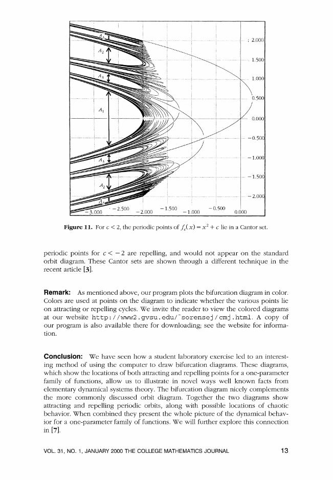
Figure 11. For c < 2 , the periodic points of fc(..c) = ..c2+ c lie in a Cantor set

periodic points for c < - 2 are repelling, and would not appear on the standard orbit diagram. These Cantor sets are shown througl~ a different technique in the recent article [ 3 ] .

Remark: As mentioned above, our prograrn plots the bifurcation diagram in color. Colors are used at points on the diagram to indicate whether the various points lie on attracting or repelling cycles. We invite the reader to view the colored diagrams at our website h t t p : / /www2 .gvsu .edu/-sorensej/ c m j .html.A copy of our program is also available there for downloading; see the website for informa- tion.

Conclusion: We have seen how a student laboratory exercise led to an interest- ing method of using the computer to draw bifurcation diagrams. These diagrams, which show the locations of both attracting and repelling points for a one-parameter family of functions, allow us to illustrate in novel ways well known facts from elernentaiy dynalnical systems theory. The bifurcation diagram nicely coinpleinents the more coininonly discussed orbit diagrain. Together the two diagrams show attracting and repelling periodic orbits, along with possible locations of chaotic behavior. When coinbitled they present the whole picture of the dynalnical behav- ior for a one-parameter family of f~inctions. We will further explore this connection in [ 7 ] .

VOL. 31, NO. 1, JANUARY 2000 THE COLLEGE MATHEMATICS JOURNAL 13

References

1. Robert L. Devaney, A First Co~~rse in Chaotic Dyi?an~ical Syster~zs: Theoly and Expei-i~neizt, Addison-\Y/esley, 1992.

2. James Gleick, Chaos: hfakiizg a ~\kzuScience, Penguin Books, 1987. 3. A. Klebanoff and J. Rickert, Studying the cantor dust at the edge of the Feigenhauln diagram, This

JOURUAL, 293 (1998) 189-197. 4. R. M. May, Simple n~athen~atical illodels w-it11 vesy complicated dynamics, ~\ratirre, 261 (1976)

459-467. 5 Lars Folii-e Olsen and Hans Degn, Chaos in biological systems, Quar-terly Reuiez~' of Biop/Jj~ic~,18:2

(1985) 165-225. 6. Heinz-Otto Peitgen, H. Ji~rgens and D. Saupe, Chaos aizd Fractals, Springer-Verlag, 1992. 7. Chip Ross and Jody Sorensen, Comparing and contrasting the orbit and bifurcation diagrams, in

preparation 8. Steven H. Strogatz, A'oizlii~ear Dyizarnics a i d C/~aos, Addison-Wesley, 1994

The Loneliness of the Long-Distance Mathematics Teacher

Kathleen Braden noticed the following in Angelu's Ashes, by Frank McCourt (Scribners's, 1996, p. 153):

Next day Brendan raises his hand. Dotty gives him the little smile. Sir, what use is Euclid and all the lines when the Germans are bombing everything that stands?

The little smile is gone. Ah, Brendan. Ah, Quigley. Oh, boys, oh, boys.

He lays his stick on the desk and stands on the platform with his eyes closed. What use is Euclid? he says. Use? Without Euclid the Messerschmitt could never have taken to the sky. Without Euclid the Spitfire could not dart from cloud to cloud. Euclid brings 11s grace and beauty and elegance. What does he bring us, boys?

Grace, sir. And? Beauty, sir. And? Elegance, sir. Euclid is cornplcte in hinlself and divine in ~ipplication. Do you

understand that, boys? We do, sir. I doubt it boys, I doubt i t . To love Euclid is to be alone in this

world. He opens his eyes and sighs and you can see the eyes are a little watery.

@THEMATHEMATICAL ASSOCIATION OF AMERICA