Wildlife responses to anthropogenic disturbance in

Amazonian forests

Mark I. Abrahams

Thesis submitted for the degree of Doctor of Philosophy

School of Environmental Sciences

University of East Anglia, Norwich, UK

September 2016

© This copy of the thesis has been supplied on the condition that anyone who consults it

is understood to recognise that its copyright rests with the author and that use of any

information derived there from must be in accordance with current UK Copyright Law.

In addition, any quotation or extract must include full attribution.

2

Contents

Acknowledgements 3

Abstract 5

Chapter 1: Introduction 6

Chapter 2: External determinants of structural and non-structural forest

disturbance along Amazonian cul-de-sac rivers 24

Chapter 3: Semi-subsistence Amazonians incur significant agricultural losses to

forest vertebrate crop raiders 73

Chapter 4: Measuring local depletion of terrestrial game vertebrates by central-

place hunters in rural Amazonia 114

Chapter 5: Trialling novel GPS units to characterise simulated hunts with

domestic dogs in Brazilian Amazonia 161

Chapter 6: Concluding Remarks 192

Photographs

Title page A várzea community in the Juruá region Chapter 1 Light aircraft flight to Carauari Chapter 2 Estrada do Gavião, Carauari Chapter 3 A proud roçado-owner in the Juruá region Chapter 4 Game carcasses and skins in the Juruá and Uatumã regions. Top left - Crax

alector, top right - Eunectes murinus, bottom left – Chelonoidis spp., bottom

right - Pecari tajacu

Chapter 5 Hunting dogs being fed Chapter 6 Sunset over the Juruá river

3

Acknowledgements

This undertaking has been a challenge and a privilege, possible only due to the multifaceted

support of many people. Firstly I thank my supervisor, Professor Carlos A. Peres, for initiating

this project and for providing guidance and inspiration throughout.

There are a host of people, communities and organisations from the Juruá and Uatumã regions, as

well as from Manaus, to whom I am immeasurably grateful. I cannot begin to thank them enough

and there are far too many for me to name them all. The incredible warmth and hospitality I was

shown in Amazonas was humbling.

The people and communities of the Juruá and Uatumã regions shared their food with me, gave me

a place to sleep, looked after me when I was sick, looked after my equipment, helped transport

me when the motor broke, worked hard with me in the forest, allowed me to work with them in

their roçados, casas de farinha, and contagem, shared outrageous stories with me (Matado por um

jabuti? Tu e doido rapas!), humoured my bizarre behaviour, tolerated my incessant questions,

terrible Portuguese and stupid mistakes, explained things patiently to me and shared with me the

beauty of their communities, the river and the forest. I don’t think I was as patient, understanding

or generous with them. I was often frustrated, tired and stressed. I hope they know how much I

appreciate all the time I spent with them. Every few weeks I still dream about the forest. It is in

my blood and I think it will always bring me back.

Many Brazilian organisations and companies provided support and datasets and enabled or

permitted me to conduct fieldwork and I am immensely grateful to them. These include the

Associação dos Moradores da Reserva de Desenvolvimento Sustentável Uacari (AMARU),

Associação dos Produtores Rurais de Carauarí (ASPROC), Centro Estadual de Unidades de

Conservação (CEUC), Fundação Amazonas Sustentável (FAS), PetroRio (formerly HRT),

Instituto Brasileiro do Meio Ambiente e dos Recursos Naturais Renováveis (IBAMA), Instituto

Chico Mendes de Conservação da Biodiversidade (ICMBio), Instituto Brasileiro de Geografia e

Estatística (IBGE), Instituto de Conservação e Desenvolvimento Sustentável da Amazônia

(IDESAM), Instituto Nacional de Pesquisas da Amazônia (INPA), Instituto de Proteção

Ambiental do Amazonas (IPAAM), Projeto Médio Juruá (PMJ), Reserva de Desenvolvimento

Sustentável do Uacari (RDS Uacari), Reserva de Desenvolvimento Sustentável do Uatumã (RDS

Uatumã), Reserva Extrativista Médio Juruá (RESEX Médio Juruá), Secretaria de Estado de Meio

Ambiente e Desenvolvimento Sustentável do Amazonas (SDS), Universidade do Estado de Mato

Grosso (UNEMAT).

My PhD studentship has been generously funded and supported by the School of Environmental

Sciences at the University of East Anglia (UEA). They provided additional unanticipated funding

for conferences and fieldwork expenses for which I am especially grateful. My fieldwork was

4 also funded by The Explorer’s Club, Idea Wild and a Darwin Initiative for the Survival of Species

grant (No. 20-001) awarded to CAP. I thank the Mataki, Technology for Nature collaboration, for

providing me with Mataki GPS devices and equipment. I thank Lucas Joppa and Siamak Tavakoli

of Microsoft Research for instigating the Mataki project.

I thank my colleague and fellow researcher Hugo C.M. Costa, for carrying out fieldwork related

to crop raiding. I also thank my colleagues at UEA, including the Centre for Ecology, Evolution

and Conservation (CEEC), for their valuable input.

I would like to thank E.J. Millner Gulland and the Imperial College Conservation Science MSc,

for giving me the opportunity to study Conservation Science. I hardly dreamed this was possible.

Lastly I thank my family, friends, officemates and girlfriend, for their unwavering support and

encouragement, and for enduring my unending expressions of frustration. My sanity is only intact

because of you.

5

Abstract

Legally inhabited indigenous, extractive and sustainable use tropical forest reserves, have been

lauded as a solution to the intractable problem of how to assure the welfare and secure livelihoods

of the world’s diverse forest-dependent people, whilst conserving the world’s most biodiverse

terrestrial ecosystems. This strategy has been critiqued by human rights advocates, who assert that

legally inhabited reserves paternalistically restrict the livelihood choices and development

aspirations of forest-dwellers, and by conservationists, who argue that sustained human presence

and resource extraction erodes tropical forest biodiversity. This thesis examines both the

anthropogenic impacts on tropical forests at the regional, landscape and household scales and the

livelihood challenges faced by semi-subsistence local communities in the Brazilian Amazon. A

spatially explicit dataset of 633,721 rural Amazonian households and an array of anthropogenic

and environmental variables were used to examine the extent and distribution of structural

(deforestation) and non-structural (hunting) human disturbance adjacent to 45 cul-de-sac rivers

across the Brazilian states of Amazonas and Pará. At the landscape and household scales, a total

of 383 camera trap deployments, 157 quantitative interviews and 164 GPS deployments were

made in the agricultural mosaics and forest areas controlled by 63 semi-subsistence communities

in the Médio Juruá and Uatumã regions of Central-Western Brazilian Amazonia, in order to

quantify and explicate the (i) livelihood costs incurred through the raiding of staple crops by

terrestrial forest vertebrates, (ii) degree of depletion that communities exert upon the assemblage

of forest vertebrates and (iii) spatial behaviour of hunting dogs and their masters during simulated

hunts. Our results indicate that at the regional scale, accessibility, fluvial or otherwise, modulated

the drivers, spatial distribution and amount of anthropogenic forest disturbance. Rural household

density was highest in the most accessible portions of rivers and adjacent to rivers close to large

urban centres. Unlike the low unipolar disturbance evident adjacent to roadless rivers, road-

intersected rivers exhibited higher disturbance at multiple loci. At the household and landscape

scales semi-subsistence agriculturalists lost 5.5% of their staple crop annually to crop raiders and

invested significant resources in lethal and non-lethal strategies to suppress crop raiders, and to

avoid losses an order of magnitude higher. Crop raiding was heightened in sparsely settled areas,

compounding the economic hardship faced by communities already disadvantaged by isolation

from urban centres. A select few harvest-sensitive species were either repelled or depleted by

human communities. Diurnal species were detected relatively less frequently in disturbed areas

close to communities, but individual species did not shift their activity patterns. Aggregate

species biomass was depressed near urban areas rather than communities. Depletion was

predicated upon species traits, with large-bodied large-group-living species the worst impacted.

Hunting dogs travelled only ~ 13% farther than their masters. Urban hunters travel significantly

farther than rural hunters. Hunting dogs were recognised to have deleterious impacts on wildlife,

but were commonly used to defend against crop raiders.

6

Chapter 1: Introduction

7

1.1 Tropical forests; importance and threats

Tropical forests have stood for some 60 million years, and harbour the majority of the Earth’s

~6.5 million terrestrial species (Burnham and Johnson, 2004, Mora et al., 2011). Yet since the

mid-1900s, roughly half of all tropical forests globally have been felled by a single species

(Fagan et al., 2006). Anthropogenic threats are simultaneously eroding tropical biodiversity and

the natural capital on which humanity depends. Apart from the immeasurable existence value of

tropical forests, they also provide a wealth of poorly quantified ecosystem services, maintaining a

biosphere amenable to human existence. These services include carbon storage, climate

regulation, water purification, and a source of novel pharmaceutical chemicals, which are crucial

to humanity in general (Costanza et al., 1997). They also provide habitat for timber and non-

timber forest resource populations, and a multi-billion dollar trade in wild-caught fish and meat

which underpins the livelihoods and subsistence of forest dwellers, who are some of the world’s

poorest people (Clay and Clement, 1993; Robinson and Bennett, 2013).

Tropical forests are also simultaneously threatened with deforestation, degradation and

defaunation. Deforestation is fuelled by population growth, colonisation and shifting global

consumption patterns (Allen and Barnes, 1985; McAlpine, et al., 2009; Schneider and Peres,

2015), enabled by road-building (Kirby et al., 2006; Adeney et al., 2009) and driven largely by

mechanized agricultural expansion (Brady, 1996; Tilman et al., 2001; Gibbs, et al., 2010),

especially for the production of beef, soy and palm oil (Fitzherbert., et al 2008; Nepstad et al.,

2014). Forest degradation results from wildfires, fragmentation, logging, livestock grazing and

biomass removal, especially for fuelwood and for charcoal production (Laurance et al., 2002,

Matricardi et al., 2010; Hosonuma et al., 2012). Lastly, anthropogenic climate change is predicted

to result in much dryer conditions in seasonally-dry tropical forests including a large portion of

the Amazon, exacerbating the aforementioned threats and potentially resulting in large-scale

habitat shifts towards lower biomass and lower diversity ecosystems (Malhi et al., 2009).

It is estimated that over 5 million tonnes of wild mammal meat is extracted annually from

Neotropical and Afrotropical forests alone (Fa and Peres, 2001). The removal of forest vertebrates

by hunters has been dubbed a “bushmeat crisis”, responsible for creating “empty forests” in

which species larger than 2kg are virtually absent (Redford, 1992; Bennett et al., 2002; Harrison,

2011). Though commercial hunters are often implicated in wildlife declines (Bowen‐Jones and

Pendry, 1999), local populations of harvest sensitive species may be severely depressed even by

isolated households of subsistence hunters (Peres, 1990). Overhunting poses both a direct threat

to the targeted species and an indirect threat to the forest as a whole. Larger-bodied, slow-

reproducing species, such as primates are especially vulnerable to overhunting (Ripple et al. in

press). The removal of large-bodied species that previously acted as ecosystem engineers and

seed dispersers (Desbiez and Kluyber, 2013; Peres et al., 2016), has far-reaching, long-term

8 consequences, deflecting some trajectories of forest regeneration more typical of faunally-intact

forests (Wilkie et al., 2011).

The impacts and even the nature of subsistence hunting in tropical forests are the subject of

divisive academic debate. Subsistence hunters are typically central place foragers, whose hunting

effort is concentrated in the first few kilometres from the household (Alvard et al., 1997). Some

argue that they behave as optimal foragers, always pursuing profitable prey regardless of prey

species vulnerability and adopting the most efficient technologies available to them, resulting in

the depletion, repulsion and extirpation of vulnerable species in multi-prey assemblages (Hawkes

et al., 1982; Mittermeier, 1987; Branch et al., 2013). Others argue that subsistence (especially

traditional) hunters have a well-developed conservation ethic, and that their selective resource and

spatial utilisation rules result in a sustainable harvest of game species (Read et al., 2010; Vliet et

al., 2010).

1.2 Social context

Nation states with sovereignty over the world’s remaining tropical forests are generally

monetarily poor and have rapidly growing and increasingly market-integrated populations

(Cincotta et al., 2000; Sachs et al., 2001). Such populations require both agricultural land and

forest timber and non-timber forest products. The effects of population growth are multiplied by

the increase in per capita consumption, which is in part a desirable consequence of declining

poverty, but also a cultural phenomenon resulting from the emulation of the unsustainable

consumerism characteristic of “developed” nations (Wilk, 1998).

Globally, and especially in tropical nations, populations have urbanised rapidly in the past century

(Cohen, 2006). This process is a mixed blessing for tropical forest conservation. By reducing the

population density in rural areas, urbanisation potentially reduces the direct pressures of both the

extraction of wild meat and agricultural clearing, and may lead to land abandonment and forest

regrowth (Cramer et al., 2008; Fearnside, 2008). Wealthier urbanites however, have a higher

disposable income and higher per capita consumption than their rural counterparts (Margulis, S.,

2004). Though direct pressure is thus reduced, the net pressure, including displaced resource-use

by urbanites, has increased. Furthermore, the local power vacuum left behind by a depopulated

countryside may render forests more vulnerable to large-scale disturbance including timber

extraction, commercial hunting (Parry et al., 2010), goldmining and petroleum extraction.

National governments and the international community have both ameliorated and exacerbated

the threats faced by tropical forests. Encouraged in part by the commitments made in the

Convention on Biological Diversity (CBD), nation states have legally protected over 13% of the

Earth’s surface (Venter et al., 2014) including 19% of the Earth’s tropical humid forest (Chape et

al., 2005). Likewise, the Convention on International Trade in Endangered Species (CITES), has

placed legal restrictions on the international trade of threatened species including mahogany

9 (Verissimo et al., 1995). Lastly, finance mechanisms including the Reducing Emissions from

Deforestation and Forest Degradation (REDD) and other Payments for Ecosystem Services (PES)

schemes including the Brazilian Bolsa Floresta, aim to harness global capital to finance the

protection of forests and their carbon in developing nations.

These measures have not been without controversy and criticism however. Efforts by the

international community to instigate strictly protected areas in tropical countries have been

branded “conservation imperialism” and “fortress conservation” (Guha, 2003; Siurua, 2006).

They are deemed hypocritical measures imposed by nations that have already enriched

themselves through wholescale ecological destruction, which threatened or devastated the

livelihoods of aborigine communities and involve grievous human rights abuses (Hutton et al.,

2005). REDD has been sharply critiqued, not only for its flawed methodology (Clements, 2010;

Watch, 2013), but because it is perceived to be an effort to simultaneously permit wealthy

polluters to continue “business as usual”, whilst disenfranchising the rural poor (Griffiths and

Martone, 2008). National governments are likewise criticised for investing tax revenues in mega-

projects with disastrous environmental and social consequences (Fearnside 1989), promoting the

exodus of neocolonists to tropical forest areas (Peres and Schneider, 2012), providing perverse

financial incentives for deforestation (Binswanger, 1991), and engaging in rest seeking behaviour

whilst colluding with illegal loggers (Palmer, 2001)

1.3 The Brazilian Amazon and its inhabitants

Though tropical regions are ecologically and socially distinct, the Brazilian Amazon exemplifies

many of the aforementioned themes. The Amazon is the largest contiguous tropical forest on

Earth, harbouring a quarter of global terrestrial biodiversity (Malhi et al., 2009) but experiences

the globally highest levels of absolute deforestation (≈2 Mha yr‒1, Laurance et al., 1998). Roughly

44% of Brazilian Amazonia falls under nonprivate conservation areas, 80.4% of the area of which

is allocated to legally inhabited reserves in which residents may pursue extractive livelihoods

(Peres, 2011)

The Brazilian Amazon is inhabited by ~25M people of diverse socio-ethnic backgrounds.

Populations are divided between sparsely inhabited hinterlands and dense cities and such as ~2M

strong Manaus, which encompasses over half of the inhabitants of the ~1.6M km2 state of

Amazonas. Amazonian urban and rural domains are however intertwined. The vast majority of

urbanites are recent migrants. Many were either born in rural communities, or still have extended

family there. As a result, rural-urban networks are maintained and multi-sited households are

common (Pinedo-Vásquez and Padoch, 2009). Many households attempt to benefit from both the

access to goods and services afforded by a town and the access to natural resources afforded by

the hinterland. These households often garner resentment from their fellow community members,

10 who consider their appropriation of land, fish and other natural resources to be excessive and

unwarranted.

Rural Amazonians include over 300,000 Indigenous Amerindians belonging to around 160

diverse linguistic and cultural groups, 50 of which are amongst the last remaining uncontacted

tribal groups on Earth (Cunha and De Almeida, 2000). The pre-Columbian Amazonian

population density is a matter of scholarly debate, but the presence of Amazonian dark earth

(terra preta. Lima et al., 2002), an anthropogenic soil created over long periods of charcoal

enrichment, indicates that in favourable locations including river bluffs and areas of fertile

floodplain (Denevan, 1996), populations were dense and longstanding. Europeans decimated the

population of Amerindians through both deliberate extermination and the introduction of novel

diseases (Roosevelt, 1997). Amerindians are still subject to deep-seated prejudice in Brazilian

society, part of which views then as an uncivilised obstacle to progress (Pallemaerts, 1986).

According to the Brazilian Institute of Geography and Statistics (IBGE) 97% of the population of

Amazonia do not identify themselves as indigenous. In the last three decades, new waves of

colonists have arrived in the Amazon from central-southern Brazil, enticed by government

subsidies and Instituto Nacional de Colonização e Reforma Agrária (INCRA) resettlement

programs (Binswanger, 1991). The majority of rural Amazonians are neither newly arrived

colonists, nor indigenous Amerindians however, but mixed heritage river dwellers (ribeirinhos),

who are the main focus of this study.

As their name suggests, ribeirinhos have settled along Amazonian waterways. Many did so in

search of rubber during the rubber boom of 1890-1930. These seringueiros (rubber tappers)

became the debt-slaves of wealthy rubber barons (patroes) who claimed monopolistic control of

river basins and extracted a rubber tithe, whilst simultaneously controlling access to goods and

services (Hvalkof, 2000). The early biopiracy of the British broke the Brazilian rubber monopoly

by creating plantations in SE Asia, which ultimately caused the crash of the Brazilian rubber

industry (Brockway, 1979). The majority of seringueiros migrated to cities during the collapse of

the rubber industry beginning in the early 1900s (Resor, 1977) but the remainder still engage in

semi-subsistence agricultural and extractive livelihoods. Freedom from patroes did not

necessarily entail prosperity. High transport costs meant that rural ribeirinhos have been prey to

regatoes, river-based merchants with a virtual monopoly on trade, who exchange manufactured

goods directly for agricultural produce at an unavoidably high price (Cleary, 1993). The increased

availability of small outboard motors (rabetas), the regional reduction in the trade of animal pelts

and skins (Bodmer et al., 1988) and the creation of producer cooperatives for farinha and rubber

within the past few decades have greatly diminished the influence of regatoes. During the 1970s,

seringueiros whose livelihoods depended on extracting resources from standing forests stood in

the way of land-seeking cattle-ranchers. The murder of human rights leader and extractive union

campaigner Chico Mendes, galvanised the movement to instate extractive and sustainable use

11 reserves to legally protect the livelihoods of extractivists and the forests on which they depend

(Fig. 1.1). Consequently, ~ 63.1 million ha of sustainable-use reserves were created in Brazilian

Amazonia since 1991 (Peres, 2011).

Figure 1.1. Examples of Amazonian extractive livelihood activities including the harvest and

processing of Euterpe oleracea (locally açaí) (A & D), fishing (B), extraction of latex rubber from

a rubber tree (Hevea brasiliensis) (C) basket weaving using Heteropsis flexuosa (locally cipó

titica) (E), extracting sawn timber (F) and a hunted Cuniculus paca (locally paca) (G) (Photos:

MIA)

12 Amazonian forests are also highly heterogeneous given their baseline geomorphological and

edaphic templates (Fig. 1.2). River basins can be classified into three types based on the chemical

properties of the river. Rivers that drain from the geologically young Andes are termed “white-

water” rivers (Sioli, 1950). They are virtually pH neutral and carry a heavy sediment load and

consequently enrich the white-water várzea floodplains during the seasonal flood pulse (Junk et

al., 1989). Rivers draining from basins dominated by sandy soils, are acidic and tannic from

partially decayed dissolved plant matter and are termed “black-water” rivers. They are bordered

by igapó forests and nutrient-poor dwarfed wooded vegetation such as campina and

campinarana. Lastly, low sediment “clear-water” rivers mostly drain from the Brazilian and

Guianan shields. River chemistry has a powerful impact on human livelihoods. Black-water rivers

have been called “hunger rivers” by their inhabitants due to nutrient-poor soils and scarcity of

wild protein sources (Janzen, 1974), though the acidic waters suppress disease vectors including

mosquitos and sandflies.

Figure 1.2. The distribution of major whitewater, blackwater, and clearwater rivers in the

Amazon basin. Source: Junk, et al., 2011

13

1.4 The Médio Juruá and Uatumã study regions

The bulk of this thesis focusses upon the Médio Juruá and Uatumã regions of Western and

Central Brazilian Amazonia, respectively, which are centred around three extractive and

sustainable use reserves. The Médio Juruá study region covers an area of 1,637,008 ha and

consists of 63.9% of primary unflooded (terra firme) forest, 30.0% of seasonally-flooded várzea

forest, 4.4% of permanent water bodies, which include the Juruá River (the second-largest white-

water tributary of the Amazon) and its tributaries and oxbow lakes, and 1.8% deforestation. Two

sustainable-use reserve - the Uacari Sustainable Development Reserve and the Médio Juruá

Extractive Reserve - jointly protect 42.3% of this landscape. The nearest towns are Carauari,

which is 88 fluvial km downriver from the Médio Juruá Reserve and has a population of 4145

families, and Itamarati, which is 120 fluvial km upstream from the Uacari Reserve and has a

population of 905 families.

The Uatumã study region covers an area of 1,601,704 ha and consists of 62.3% of undulating

upland primary unflooded (terra firme) forest, 17.9% of primary low-lying and seasonally-

flooded igapo forest, 11.1% permanent water bodies, which include the Uatumã River (which

connects the Balbina reservoir to the Amazon River) and its main tributary the Jatapú River, 4.0%

deforestation and 4.7% of campina and campinarana non-forest vegetation on oligotrophic soils.

The Uatumã Sustainable Development Reserve legally protects 27.0% of this landscape. The

nearest towns are Vila Balbina, which has a population of 420 families and is 66 fluvial km

upstream of the reserve, and Sao Sebastião, Itapiranga and Urucará, with populations of 1214,

1345 and 2051 families, respectively, and are 37, 40, and 53 fluvial km downriver of the reserve,

respectively.

Both regions are inhabited by ribeirinhos, with producer cooperatives and resource-management

programs. Large-scale ecological and socioeconomic differences between the two study regions

are due to river chemistry and proximity to Manaus, the largest city in Brazilian Amazonia. The

Juruá region encompasses white-water floodplain ecosystems, whereas the Uatumã region

encompasses black-water ecosystems. Secondly, the Juruá region is over five times farther from

Manaus, which increases transaction costs and reduces market opportunities for Juruá inhabitants.

Manioc (Manihot esculenta) is the staple source of carbohydrates in our study regions, as in much

of the humid tropics (Cock, 1982; Frazer, 2010). Crops including maize and bananas are also

locally important, but their higher nutrient requirements prevent their large scale cultivation in

most of Amazonia. The main varieties of manioc are high-cyanide manioc (Peroni et al., 2007),

locally called “roça brava”, and low-cyanide manioc, locally called “macaxeira”. M. esculenta

produces large tubers, tolerates poor tropical soils and is pest-resistant. Manioc is processed in a

flour-house (locally “casa de farinha”) into a relatively imperishable, high calorie course flour

(locally “farinha”) (Fig. 1.3). Communities grow manioc in swidden agricultural plots called

14 roçados, often representing the main livelihood activity for semi-subsistence riparian

communities in the lowland Amazon (Newton et al., 2012). Roçados are generally active for 4

years until weed encroachment and declining soil fertility force their abandonment (Unruh, 1988).

The resulting secondary forests (locally “capoeiras”) are then left to undergo successional

regrowth until standing biomass and soil nutrient loads are sufficient to permit re-clearing. This

shifting agriculture process creates a mosaic of habitats under different successional stages

around village settlements, with shorter-rotation plots generally closer to the community (Coomes

et al., 2000).

Figure 1.3. The cultivation and processing of manioc (Manihot esculenta). A cleared and burned

agricultural plot (roçado) with immature manioc plants (A) and maturing manioc plants (B). The

peeling (C), grinding, sieving and roasting (D) of manioc into farinha. (Photos: MIA)

15

1.5 The challenge of sustainable use

Amazonian sustainable use and extractive reserves were created with the dual purpose of

maintaining human extractive livelihoods, as well as protecting the biodiverse forest ecosystems

upon which those livelihoods depend. Many conservationists consider these dual aims to be in

conflict. They argue that human occupation of protected areas inevitably results in habitat

degradation and species extirpation and that biodiversity is best served through the enforcement

of strictly protected areas (Kramer et al., 1997, Brandon et al., 1998).

Figure 1.4. Examples of natural resource management programs in the Juruá region. The

monitoring of river turtle (Podocnemis spp.) nesting beaches (A) and the offtake of pirarucu

(Arapaima gigas) from managed oxbow lakes (B). (Photos: MIA)

Many tropical forest resources, including timber and wild-caught game animals and fish are

classic examples of common pool resources (Ostrom, 2005) in that they are both rivalrous and

non-excludable. This makes them especially vulnerable to a ‘tragedy of the commons’, in which

all users are incentivised to extract as much as possible, leading to stock collapses. Such collapses

are indeed evident in stocks of timber and of certain large-bodied species of fish regionally

(Castello et al., 2011; Richardson and Peres, 2016) and locally for populations of Brazilian

Rosewood (pau rosa) in the Uatumã region and of pirarucú (Arapaima gigas) and river turtles

(Podocnemis spp.) in the Juruá region (but see Campos-Silva & Peres 2016). Recent community

resource management programs for pirarucu in the Juruá region have however proven effective at

restoring fish stock (Silva, 2014). Pirarucú, congregate in oxbow lakes, seasonally detached from

the main river during the low water season, and occasionally surface to breathe. This facilitates

both their monitoring and the exclusion of non-residents (Fig. 1.4). In addition, the Bolsa Floresta

16 program, managed by the Fundação Amazonas Sustentável (FAS) is a payments for ecosystem

services (PES) scheme that incentivises communities to avoid deforesting primary forest and to

implement timber stock management strategies (Vianna and Fearnside, 2014).

The management of subsistence hunting has however proven a greater challenge. Many of the

large and highly prised game species such as South American tapir, are far less productive than

even large aquatic species, such that their populations are likely to respond more slowly to offtake

management. Furthermore, populations of terrestrial game species are difficult to locally monitor

(Munari et al., 2011, Constantino et al., 2012) and excluding hunters from the forests they inhabit

is virtually impossible. As part of a government-funded resource management program

(Programa de Monitoramento da Biodiversidade e do Uso de Recursos Naturais em Unidades de

Conservação Estaduais do Amazonas, ProBUC) and the Projeto Médio Juruá (led by Prof CA

Peres, University of East Anglia), line transect surveys have been conducted in both the Juruá and

Uatumã regions as a means of faunal monitoring. As a means of monitoring hunted populations,

line-transects surveys have however been criticised for their detectability biases, because hunted

species are known to change their behaviour in response to persistent hunting and other

anthropogenic disturbance, such that they become less detectable (Johns, 1985). Though the use

of camera trapping rates to infer relative abundance is not without problems (Sollmann et al.,

2013), camera traps are becoming ubiquitous tools in conservation and ecology (Rowcliffe and

Carbone, 2008) and they potentially offer a monitoring solution that circumvents species

behavioural responses to human surveyors.

1.6 Aims and thesis structure

The overarching aim of this study on wildlife responses to anthropogenic disturbance in

Amazonian forests, was to examine the degree to which current human occupation and extractive

use of tropical forests is compatible with biodiversity conservation. To that end, research was

carried out at the regional, landscape and community scales, and encompassed both the

ecological/biotic impacts of human activities, and the conflicts generated by human livelihoods

and extractive practices. This study was developed in response to the threats to tropical forests

identified above, and the potential for legally inhabited sustainable use and extractive reserves to

serve dual social and conservation purposes.

The four data chapters of this thesis were written in manuscript format, with the intention of

publishing each separately as articles in peer-reviewed journals. As such, each chapter contains its

own reference list and appendices and some repetition is unavoidable in material within the

methods sections.

Chapter 2: A regional-scale approach and Geographic Information System (GIS) tools were used

to quantify and compare patterns of structural and non-structural anthropogenic disturbance

17 across 45 cul-de-sac roadless and road-intersected navigable rivers throughout the states of

Amazonas and Pará. Whole-river and fluvial-segment analyses were employed to elucidate

within-river and between-river patterns. The relative importance of environmental, local and non-

local anthropogenic factors in driving forest disturbance, was discussed.

Chapter 3: The prevalence and livelihood impacts of terrestrial vertebrate crop-raiding damage

to manioc semi-subsistence agricultural plots in the Médio-Juruá region was quantified,

contextualized and explained using camera traps and structured interviews. The degree to which

subsistence hunting gains are sufficient to offset losses to crop raiders, as well as the

complementarity of social and ecological research approaches, were discussed.

Chapter 4: Camera traps and structured interviews were used to survey the peri-community areas

controlled by semi-subsistence communities in both the Médio Juruá and Uatumã regions, in

order to quantify envelopes of depletion of forest vertebrates in proximity to human communities.

The anthropogenic impacts on the detection rates of individual species, the aggregate biomass of

forest vertebrates and on faunal activity patterns, at both the community and landscape scale,

were assessed. The extent to which community-based subsistence offtake is compatible with

ecologically functional populations of tropical forest game species, was discussed.

Chapter 5: The spatial behaviour of hunting dogs and their masters during simulated hunts in the

Juruá and Uatumã regions, was characterised. The effectiveness of novel GPS units was

compared to that of commercially available alternatives. The ecological costs and social benefits

of the use of hunting dogs, were discussed.

Chapter 6: The main findings of the four data chapters were summarised. Themes common to the

four data chapters were synthesised and discussed. Lastly, potential conservation strategies and

fruitful areas of future research were indicated.

18

1.7 References

Alvard, M.S., Robinson, J.G., Redford, K.H. and Kaplan, H., 1997. The sustainability of

subsistence hunting in the Neotropics. Conservation Biology, 11(4), pp.977-982.

Bennett, E.L., Eves, H.E., Robinson, J.G. and Wilkie, D.S., 2002. Why is eating

bushmeat a biodiversity crisis? Conservation Biology In Practice, 3, pp.28-29.

Binswanger, H.P., 1991. Brazilian policies that encourage deforestation in the

Amazon. World Development, 19(7), pp.821-829.

Bodmer, R.E., Fang, T.G. and Ibanez, L.M., 1988. Ungulate management and

conservation in the Peruvian Amazon. Biological Conservation, 45(4), pp.303-310.

Branch, T.A., Lobo, A.S. and Purcell, S.W., 2013. Opportunistic exploitation: an

overlooked pathway to extinction. Trends in Ecology & Evolution, 28(7), pp.409-413.

Brandon, K., Redford, K.H. and Sanderson, S.E. eds., 1998. Parks in peril: people,

politics, and protected areas (No. 333.783 P252). Washington, DC: Island Press.

Brockway, L.H., 1979. Science and colonial expansion: the role of the British Royal

Botanic Gardens. American Ethnologist, 6(3), pp.449-465.

Burnham, R.J. and Johnson, K.R., 2004. South American palaeobotany and the origins of

neotropical rainforests. Philosophical Transactions of the Royal Society B: Biological

Sciences, 359(1450), pp.1595-1610.

Campos-Silva, J. V. and Peres, C. A. Community-based management induces rapid

recovery of a high-value tropical freshwater fishery. Scientific Reports. 6, 34745; doi:

10.1038/srep34745 (2016).

Castello, L., McGrath, D.G. and Beck, P.S., 2011. Resource sustainability in small-scale

fisheries in the Lower Amazon floodplains. Fisheries Research,110(2), pp.356-364.

Chape, S., Harrison, J., Spalding, M. and Lysenko, I., 2005. Measuring the extent and

effectiveness of protected areas as an indicator for meeting global biodiversity

targets. Philosophical Transactions of the Royal Society of London B: Biological

Sciences, 360(1454), pp.443-455.

Cincotta, R.P., Wisnewski, J. and Engelman, R., 2000. Human population in the

biodiversity hotspots. Nature, 404(6781), pp.990-992.

Clay, J.W. and Clement, C.R., 1993. Selected species and strategies to enhance income

generation from Amazonian forests. Rome: Food and Agriculture Organization of the United

Nations.

19

Cleary, D., 1993. After the frontier: Problems with political economy in the modern

Brazilian Amazon. Journal of Latin American Studies, 25(02), pp.331-349.

Clements, T., 2010. Reduced expectations: the political and institutional challenges of

REDD+. Oryx, 44(03), pp.309-310.

Cohen, B., 2006. Urbanization in developing countries: Current trends, future projections,

and key challenges for sustainability. Technology in Society, 28(1), pp.63-80.

Constantino, P.D.A.L., Carlos, H.S.A., Ramalho, E.E., Rostant, L., Marinelli, C.E., Teles,

D., Fonseca-Junior, S.F., Fernandes, R.B. and Valsecchi, J., 2012. Empowering local people

through community-based resource monitoring: a comparison of Brazil and Namibia. Ecology

and Society, 17(4), p.22.

Costanza, R., d'Arge, R., De Groot, R., Faber, S., Grasso, M., Hannon, B., Limburg, K.,

Naeem, S., O'neill, R.V., Paruelo, J. and Raskin, R.G., 1997. The value of the world's ecosystem

services and natural capital. The Globalization and Environment Reader, p.117.

Cramer, V.A., Hobbs, R.J. and Standish, R.J., 2008. What's new about old fields? Land

abandonment and ecosystem assembly. Trends in Ecology & Evolution, 23(2), pp.104-112.

Denevan, W.M., 1996. A bluff model of riverine settlement in prehistoric

Amazonia. Annals of the Association of American Geographers, 86(4), pp.654-681.

Desbiez, A.L.J. and Kluyber, D., 2013. The role of giant armadillos (Priodontes

maximus) as physical ecosystem engineers. Biotropica, 45(5), pp.537-540.

Fa, J.E. and Peres, C.A., 2001. Game vertebrate extraction in African and Neotropical

forests: an intercontinental comparison. Conservation Biology Series-Cambridge-, pp.203-241.

Fa, J.E., Peres, C.A. and Meeuwig, J., 2002. Bushmeat exploitation in tropical forests: an

intercontinental comparison. Conservation Biology, 16(1), pp.232-237.

Fagan, C., Peres, C.A. and Terborgh, J., 2006. Tropical forests: a protected-area strategy

for the twenty-first century. In Lawrence, W. F. and Peres, C. A. (Eds.). Emerging threats to

tropical forests, pp. 415–432. University of Chicago Press, Chicago, pp.415-432.

Fearnside, P.M., 1989. Brazil's Balbina Dam: Environment versus the legacy of the

pharaohs in Amazonia. Environmental Management, 13(4), pp.401-423.

Fearnside, P.M., 2008. Will urbanization cause deforested areas to be abandoned in

Brazilian Amazonia?. Environmental Conservation, 35(03), pp.197-199.

Fitzherbert, E.B., Struebig, M.J., Morel, A., Danielsen, F., Brühl, C.A., Donald, P.F. and

Phalan, B., 2008. How will oil palm expansion affect biodiversity?. Trends in Ecology &

Evolution, 23(10), pp.538-545.

20

Goulding, M., Barthem, R. and Ferreira, E., 2003. The Smithsonian atlas of the Amazon.

Smithsonian Books. Washington and London.

Griffiths, T. and Martone, F., 2008. Seeing ‘REDD’. Forests, climate change mitigation

and the rights of indigenous peoples and local communities. Update for Poznan (UNFCCC COP

14). Forest Peoples Programme, Moretonin-Marsh, UK.

Guha, R., 2003. The authoritarian biologist and the arrogance of anti-humanism: wildlife

conservation in the Third World. Battles over nature: Science and politics of conservation.

Permanent Black, New Delhi, India, pp.139-157.

Hawkes, K., Hill, K. and O'Connell, J.F., 1982. Why hunters gather: optimal foraging and

the Ache of eastern Paraguay. American Ethnologist, 9(2), pp.379-398.

Hosonuma, N., Herold, M., De Sy, V., De Fries, R.S., Brockhaus, M., Verchot, L.,

Angelsen, A. and Romijn, E., 2012. An assessment of deforestation and forest degradation drivers

in developing countries. Environmental Research Letters, 7(4), p.044009.

Hutton, J., Adams, W.M. and Murombedzi, J.C., 2005, December. Back to the barriers?

Changing narratives in biodiversity conservation. In Forum for development studies (Vol. 32, No.

2, pp. 341-370). Taylor & Francis Group.

Hvalkof, S., 2000. Outrage in rubber and oil: Extractivism, indigenous peoples, and

justice in the Upper Amazon in Zerner, C., People, plants, and justice: the politics of nature

conservation. Columbia University Press.

Janzen, D.H., 1974. Tropical blackwater rivers, animals, and mast fruiting by the

Dipterocarpaceae. Biotropica, pp.69-103.

Junk, W.J., 1984. Ecology of the várzea, floodplain of Amazonian whitewater rivers.

In The Amazon (pp. 215-243). Springer Netherlands.

Junk, W.J., Bayley, P.B. and Sparks, R.E., 1989. The flood pulse concept in river-

floodplain systems. Canadian Special Publication of Fisheries and Aquatic Sciences, 106(1),

pp.110-127.

Junk, W.J., Piedade, M.T.F., Schöngart, J., Cohn-Haft, M., Adeney, J.M. and Wittmann,

F., 2011. A classification of major naturally-occurring Amazonian lowland

wetlands. Wetlands, 31(4), pp.623-640.

Kramer, R., van Schaik, C. and Johnson, J. (eds)., 1997. Last stand: protected areas and

the defense of tropical biodiversity. Oxford University Press.

21

Laurance, W.F., Lovejoy, T.E., Vasconcelos, H.L., Bruna, E.M., Didham, R.K., Stouffer,

P.C., Gascon, C., Bierregaard, R.O., Laurance, S.G. and Sampaio, E., 2002. Ecosystem decay of

Amazonian forest fragments: a 22‐year investigation. Conservation Biology, 16(3), pp.605-618.

Lima, H.N., Schaefer, C.E., Mello, J.W., Gilkes, R.J. and Ker, J.C., 2002. Pedogenesis

and pre-Colombian land use of “Terra Preta Anthrosols”(“Indian black earth”) of Western

Amazonia. Geoderma, 110(1), pp.1-17.

Malhi, Y., Aragão, L.E., Galbraith, D., Huntingford, C., Fisher, R., Zelazowski, P., Sitch,

S., McSweeney, C. and Meir, P., 2009. Exploring the likelihood and mechanism of a climate-

change-induced dieback of the Amazon rainforest. Proceedings of the National Academy of

Sciences,106(49), pp.20610-20615.

Margulis, S., 2004. Causes of deforestation of the Brazilian Amazon (Vol. 22). World

Bank Publications.

Matricardi, E.A., Skole, D.L., Pedlowski, M.A., Chomentowski, W. and Fernandes, L.C.,

2010. Assessment of tropical forest degradation by selective logging and fire using Landsat

imagery. Remote Sensing of Environment, 114(5), pp.1117-1129.

McAlpine, C.A., Etter, A., Fearnside, P.M., Seabrook, L. and Laurance, W.F., 2009.

Increasing world consumption of beef as a driver of regional and global change: A call for policy

action based on evidence from Queensland (Australia), Colombia and Brazil. Global

Environmental Change, 19(1), pp.21-33.

Mittermeier, R.A., 1987. Effects of hunting on rain forest primates. in C. Marsch, R.A.

Mittermeier (Eds.), Primate Conservation in the Tropical Rain Forest, Alan R. Liss, New York

(1987), pp. 109–146

Mora, C., Tittensor, D.P., Adl, S., Simpson, A.G. and Worm, B., 2011. How many

species are there on Earth and in the ocean?. PLoS Biology, 9(8), p.e1001127.

Munari, D.P., Keller, C. and Venticinque, E.M., 2011. An evaluation of field techniques

for monitoring terrestrial mammal populations in Amazonia. Mammalian Biology-Zeitschrift für

Säugetierkunde, 76(4), pp.401-408.

Naughton-Treves, L., Holland, M.B. and Brandon, K., 2005. The role of protected areas

in conserving biodiversity and sustaining local livelihoods. Annual Review of Environment and

Resources. 30, pp.219-252.

Nepstad, D., McGrath, D., Stickler, C., Alencar, A., Azevedo, A., Swette, B., Bezerra, T.,

DiGiano, M., Shimada, J., da Motta, R.S. and Armijo, E., 2014. Slowing Amazon deforestation

through public policy and interventions in beef and soy supply chains. Science, 344(6188),

pp.1118-1123.

22

Ostrom, E., 2005. Self-governance and forest resources. Terracotta reader: a market

approach to the environment. Academic Foundation, New Delhi, pp.131-155.

Pallemaerts, M., 1986. Development, conservation, and indigenous rights in

Brazil. Human Rights Quarterly, 8(3), pp.374-400.

Palmer, C., 2001. The extent and causes of illegal logging: an analysis of a major cause

of tropical deforestation in Indonesia. Centre for Social and Economic Research on the Global

Environment (CSERGE): London, UK

Parry, L., Peres, C.A., Day, B. and Amaral, S., 2010. Rural–urban migration brings

conservation threats and opportunities to Amazonian watersheds. Conservation Letters, 3(4),

pp.251-259.

Peres, C.A. and Schneider, M., 2012. Subsidized agricultural resettlements as drivers of

tropical deforestation. Biological Conservation, 151(1), pp.65-68.

Peres, C.A., 2011. Conservation in Sustainable‐Use Tropical Forest

Reserves. Conservation Biology, 25(6), pp.1124-1129.

Peres, C.A., Emilio, T., Schietti, J., Desmoulière, S.J. and Levi, T., 2016. Dispersal

limitation induces long-term biomass collapse in overhunted Amazonian

Pinedo-Vásquez, M. and Padoch, C., 2009. Urban and rural and in-between: Multi-sited

households, mobility and resource management in the Amazon floodplain. Mobility and

migration in indigenous Amazonia: Contemporary Ethnoecological Perspectives, 11, pp.86-96.

Read, J.M., Fragoso, J.M., Silvius, K.M., Luzar, J., Overman, H., Cummings, A., Giery,

S.T. and de Oliveira, L.F., 2010. Space, place, and hunting patterns among indigenous peoples of

the Guyanese Rupununi region. Journal of Latin American Geography, 9(3), pp.213-243.

Redford, K.H., 1992. The empty forest. BioScience, 42(6), pp.412-422.

Resor, R.R., 1977. Rubber in Brazil: Dominance and collapse, 1876-1945. Business

History Review, 51(03), pp.341-366.

Richardson, V.A. and Peres, C.A., 2016. Temporal Decay in Timber Species

Composition and Value in Amazonian Logging Concessions. PloS one, 11(7), p.e0159035.

Ripple, W.J., Abernethy, K, Chapron, G., Dirzo, R., Galetti, M., Levi, T., Lindsey, P.A.,

Macdonald, D.W., Newsome, T.M., Peres, C.A., Wallach, C.W., and Young, H., In press. Are we

eating the world’s mammals to extinction? Royal Society Open Science

Robinson, J.G. and Bennett, E.L., 2013. Hunting for sustainability in tropical forests.

Columbia University Press.

23

Roosevelt, A. ed., 1997. Amazonian indians from prehistory to the present:

anthropological perspectives. University of Arizona Press.

Rowcliffe, J.M. and Carbone, C., 2008. Surveys using camera traps: are we looking to a

brighter future?. Animal Conservation, 11(3), pp.185-186.

Silva, M.D.C., 2014. Análise do Manejo Comunitário de Pirarucu (Arapaima Spp.) Na

Resex Médio Juruá e Rds Uacari, Município de Carauari, Amazonas, Brasil.

Sioli, H., 1950. Das wasser im Amazonasgebiet. Forsch. Fortschr, 26(21/22), pp.274-

Siurua, H., 2006. Nature above people: Rolston and" fortress" conservation in the

South. Ethics & the Environment, 11(1), pp.71-96.

Tockman, J., 2001. The International Monetary Fund: Funding deforestation.

Washington: American Lands Alliance.

Van Vliet, N., MILNER‐GULLAND, E.J., Bousquet, F., Saqalli, M. and Nasi, R., 2010.

Effect of Small‐Scale Heterogeneity of Prey and Hunter Distributions on the Sustainability of

Bushmeat Hunting. Conservation Biology, 24(5), pp.1327-1337.

Venter, O., Fuller, R.A., Segan, D.B., Carwardine, J., Brooks, T., Butchart, S.H., Di

Marco, M., Iwamura, T., Joseph, L., O'Grady, D. and Possingham, H.P., 2014. Targeting global

protected area expansion for imperiled biodiversity. PLoS Biology, 12(6), p.e1001891.

Verissimo, A., Barreto, P., Tarifa, R. and Uhl, C., 1995. Extraction of a high-value

natural resource in Amazonia: the case of mahogany. Forest Ecology and Management, 72(1),

pp.39-60.

Vianna, A.L.M. and Fearnside, P.M., 2014. Impact of community forest management on

biomass carbon stocks in the Uatumã Sustainable Development Reserve, Amazonas,

Brazil. Journal of sustainable forestry, 33(2), pp.127-151.

Watch, C.T., 2013. Protecting Carbon to destroy forests. Land enclosures and

REDD+. Carbon Trade Watch.

Wilk, R., 1998. Emulation, imitation, and global consumerism. Organization &

Environment, 11(3), pp.314-333.

Wilkie, D.S., Bennett, E.L., Peres, C.A. and Cunningham, A.A., 2011. The empty forest

revisited. Annals of the New York Academy of Sciences, 1223(1), pp.120-128.

24

Chapter 2: External determinants of structural and non-structural

forest disturbance along Amazonian cul-de-sac rivers

Submitted to Global Environmental Change as:

Abrahams, M.I., and Peres, C.A. Human and physical geography modulate structural and non-

structural anthropogenic forest disturbance along Amazonian cul-de-sac rivers

25

Abstract

Infrastructure development in the Brazilian Amazon continues apace, opening new frontiers into

hitherto remote, previously undisturbed areas, yet the spatial extent of different patterns of

human-induced structural (deforestation) and non-structural (hunting) disturbance in tropical

forest regions is yet to be investigated simultaneously. This study examines an aggregate area of

301,641 km² adjacent to 45 cul-de-sac rivers across the Brazilian states of Amazonas and Pará.

These rivers represent the interface between highly accessible fluvial highways and remote forest

headwaters across Amazonia, which are becoming integrated to varying degrees into an

expanding network of roads and towns, eroding their inaccessibility. We use a spatially explicit

dataset of 633,721 rural Amazonian households and an array of anthropogenic and environmental

variables to firstly quantify and compare patterns of structural and non-structural anthropogenic

disturbance, and to secondly examine correlates of deforestation such as rural population density,

one of the hypothesised primary drivers of disturbance. Comparing structural and non-structural

disturbance, our findings conservatively suggest that non-structural disturbance accounts for an

area over eighteen times larger than structural disturbance. Our analyses also confirm that

accessibility modulates the drivers, spatial distribution and amount of tropical forest disturbance.

Rural household density was highest adjacent to rivers whose mouths are close to large urban

centres in their most accessible portions. Roadless rivers succumbed to low, unipolar disturbance,

whilst road-intersected rivers exhibited higher disturbance footprints at multiple loci. These

results suggest that the development trajectory chosen by lowland tropical forest countries can

have far-reaching implications for biodiversity.

26

2.1 Introduction

Despite the fact that tropical forests simultaneously harbour the majority of global terrestrial

biodiversity and provide ecosystem services crucial to humanity (Naidoo et al., 2008), they

continue to be converted or degraded by multiple anthropogenic threats (Wright, 2010). Land-use

change is arguably the most significant global scale driver of terrestrial biodiversity loss (Sala, et

al., 2000). Habitat conversion due to agricultural expansion is identified as the principal

mechanism (Tilman et al., 2001) and tropical forests bear the brunt of the damage (Gibbs, et al.,

2010). The degradation and conversion of tropical forests entails a staggering biotic simplification

across multiple taxa (Barlow et al., 2007; Gibson, et al., 2011). On the other hand, merely

preventing habitat conversion is insufficient to safeguard tropical biodiversity. Although

superficially intact tropical forests may appear to be an unbroken impenetrable mat stretching in

all directions, this seductive picture may mask an eerily silent “empty forest” (Redford, 1992) in

which species larger than 2kg may be virtually absent due to overhunting (Harrison, 2011).

Retaining merely structurally intact forests may thus be a Pyrrhic victory, especially if the loss of

functionally crucial taxa results in continued long-term tropical forest degradation (Peres et al.,

2016).

The Amazon rainforest, 62% of which falls within Brazil, harbours roughly a quarter of global

terrestrial biodiversity (Malhi et al., 2009) and is the largest contiguous tropical forest on Earth.

The Brazilian Amazon experiences the globally highest levels of absolute deforestation (≈2 Mha

yr‒1, Laurance et al., 1998). The “Amazonia Legal” region within Brazil covers an area of ≈

508,788,238 ha, over 25% of which is protected by legally inhabited reserves including

indigenous, sustainable use and extractive reserves (de Marques, et al., 2016; IUCN and UNEP-

WCMC (2015)) and an additional 21% are protected by indigenous territories.

Cul-de-sac wilderness rivers are pivotal in strategies to protect tropical biodiversity, and can be

defined as rivers which do not act as thoroughfares between urban centers (Appendix A). In

Amazonia, they are typically first- and second-order tributaries that link major fluvial highways

including the Amazonas/Solimões, Negro and Madeira Rivers, with remote and largely

uninhabited headwater regions, which retain some of the last remaining tracts of inaccessible

tropical forest wildlands on Earth (Peres and Lake, 2003). The unidirectional accessibility of cul-

de-sac rivers imposes livelihood constraints on their inhabitants, limiting the spread of

anthropogenic disturbance to the lower portions of river basins. The influence of urban centres

and the expansion of road networks, however, is beginning to erode their isolation. In particular,

the advance of deforestation frontiers along the “arc of deforestation” has culminated in a highly

modified forest mosaic in eastern and southern Amazonia. The development of the Trans-

Amazon Highway in the 1970s, enabled colonists to bypass fluvial navigational constraints and

access hitherto inaccessible forest areas. Brazilian development policy and especially the perverse

27 subsidies and encouragement (by the Instituto Nacional de Colonização e Reforma Agrária

(INCRA)) of Amazonian colonisation, have actively fuelled this movement (Binswanger, 1991).

Brazilian government commitments to develop hinterland infrastructure colluded with foreign

interests is paving the way for extractive industries based of mineral resources (Reid and De

Sousa, 2005; Ferreira et al. 2015), and make it likely that even currently remote areas will be

affected.

Rural extractive communities and isolated households are the only inhabitants of long stretches of

cul-de-sac Amazonian rivers. Rural Amazonians are not homogenous, but fall on a socio-ethnic

spectrum (Chibnik, 1991) between; (1) Indigenous Amerindian peoples, who have occupied

Amazonia for some 10,000 years (Miller, and Nair, 2006). Numbering over 300,000 people, they

belonging to around 160 diverse linguistic and cultural groups, ~50 of which are amongst the last

remaining uncontacted tribal groups on Earth (Cunha and De Almeida, 2000), but are collectively

referred to as indians (índios); (2) Neo-colonist groups of mixed European and African descent

who migrated into the Amazon within the last three generations, often collectively referred to as

colonos; and (3) Groups of mixed Amerindian and non-Amerindian descent whose ethnicity,

identity, culture and livelihood practices are an intermediate mixture between the aforementioned

groups, who are often referred to as river dwelling caboclos or ribeirinhos.

Rural Amazonian livelihood strategies likewise fall on a spectrum between self-sufficient

subsistence extractivism and market-integrated agricultural production. Whilst most households

engage in both to varying degrees (Newton et al., 2012), high degrees of market integration are

often associated with more recent colonists (Stocks et al., 2007; Lu et al., 2010). Horticultural

practices and small-livestock husbandry are largely restricted to comparatively small, heavily

modified areas close to homesteads to maximise production and minimise travel costs. By

contrast, extractive livelihood practices for subsistence, including hunting and harvesting of other

nontimber forest products, require extensive catchment areas. Hunters range over large areas and

capture widely distributed and highly mobile prey, without directly modifying forest structure in

the short term (but see Peres et al., 2016). As predicted by bid-rent theory (Von Thünen, 1966),

households engaging primarily in agricultural production, prioritise proximity to urban centers to

minimise transport and exchange costs, whereas those engaging primarily in subsistence

extractivism, who occupy what Von Thünen termed the “wilderness”, prioritise access to natural

resources under lower competitive arenas.

Over 97% of Brazilian Amazonians are non-tribal, and typically of non-indigenous descent

(IBGE, 2008). Though often occupying remote areas and adopting elements of indigenous

livelihood practices, most ribeirinhos are integrated to varying degrees into the Brazilian

economy and society and depend on state infrastructure and market goods and services. They are

therefore influenced by large-scale sociopolitical and economic processes such as the waxing and

waning of the rubber industry, which impelled them to settle remote headwaters with its rise and

28 drew them back into urban areas with its collapse (Hecht and Cockburn, 2010, Parry et al.,

2010a). Recent government welfare programs and subsidies, such as “Bolsa Familia”, “Luz Para

Todos” and “Minha Casa Minha Vida”, have somewhat mitigated the rural exodus.

Different forms of human-induced disturbance in tropical forest regions are almost always

considered separately in the conservation science literature (Laurence and Peres, 2006). To our

knowledge no study has analysed the threats of both hunting and deforestation in the context of

cul-de-sac tropical forest rivers (but see Parry et al 2010b for an analysis of extractive activities

along eight roadless cul-de-sac rivers). This study uses an array of spatially explicit human

population and environmental datasets, including the locations of 633,721 rural Amazonian

households, to, firstly, quantify two widespread forms of human structural and non-structural

disturbance in tropical forest regions, deforestation and hunting, associated with 45 cul-de-sac

rivers. These rivers represent ~ 23,000 km of fluvial distance associated with an area of over

301,000 km². Secondly, we examine the relative importance of local and external anthropogenic

and environmental factors in explaining the extent of deforestation and hunting. Finally, we

discuss the conservation implications of large-scale infrastructure development and socio-

demographic changes in Amazonia. By examining truly unipolar rivers alongside those with a

degree of road connectivity, we hope to provide insights into the future of an increasingly

accessible Amazon.

Due to differences in the aforementioned livelihood practices, we hypothesise that structural

disturbance will encompass a small subset of the area affected by non-structural disturbance. We

anticipate that highly detectable forest disturbance, will be concentrated near loci of access to

external centers of services and trade. Along roadless rivers these loci will be located at river

mouths accessible to market towns. By contrast, rivers bisected by roads in their upper sections,

along which agricultural settlements have developed in the last three decades, will exhibit a more

bimodal pattern of disturbance.

Due to the inaccessibility of our study river-basins, we hypothesise that rural households are the

main agents of disturbance along these rivers and that rural population density is the main

predictor of disturbance. In addition to population density, the spatial configuration of rural

settlements, should also affect patterns of disturbance. Small and large-scale household clustering

increases pseudo-interference and exploitative competition (McGinley, 2008, Levi et al., 2009),

causing hunting catchments to coalesce and therefore reducing the overall hunting footprint and

lowering rates of disturbance per household.

As rural households can rely on both extractivism and agriculture, and assuming that rural

settlements approximate an ideal-free distribution (as in rural communities elsewhere: Moritz et

al., 2014), we hypothesize that both environmental and anthropogenic factors drive rural

population density, with a higher household density along rivers with more abundant natural

resources and easier access to markets. Anthropogenic factors such as roads, increase disturbance

29 both directly and indirectly by increasing rural population density, whereas environmental factors

indirectly affect disturbance by either enabling or hindering both rural populations and external

actors. For further discussion of the individual hypothesised drivers of disturbance in our study

area, see Appendix K.

2.2 Methods

2.2.1 Study area

Our analysis focuses on 45 navigable cul-de-sac rivers distributed across the two largest states in

Brazil, representing the largest tropical forest sub-national divisions on Earth, Amazonas and Pará

(Fig. 2.1). The former has a total population of 3,938,336, encompasses 157,128,871 ha, has

experienced only ~2% deforestation (PRODES, 2009), and has an overall mean rural human

population density of ~0.4 inhabitants per km² (IBGE, 2008). The state of Pará has a total

population of 7,792,561, covers 124,836,546 ha, has a mean rural population density of ~1.5

inhabitants per km² (IBGE, 2008) and has experienced a deforestation rate that is roughly ten-fold

higher (~20%). Mean road density (km/km², including major unpaved roads) across the states of

Amazonas and Pará is approximately 0.00219 and 0.00981, respectively. Given Brazil’s

economic trajectory in frontier expansion and geopolitical commitments to develop the Amazon

using massive tax-payer investments (Laurance et al., 2001; Peres, 2001), conservationists often

project the future of Amazonas as analogous to present-day Pará. Insights gained from the latter

can therefore inform future conservation and development policies in the former.

30

Figure 2.1: Study area in the Brazilian Amazon, showing the distribution of 45 studied cul-de-sac

rivers selected in this study (white, black and blue lines representing white-water, black-water and

clear-water rivers, respectively) against a background of land-cover classification in which green

indicates forest, red indicates deforestation, peach indicates natural non-forest vegetation, and

blue indicates water-bodies (PRODES 2009). Number codes next to rivers correspond to those

listed in Table 2.1. Areas outside Brazil are indicated in grey and state boundaries are represented

by dark grey lines. Manaus, the capital of the state of Amazonas, is indicated by a black circle.

Inset map shows continental scale location of the study area.

2.2.1 GIS integration and analysis

All GIS data extraction and analysis was undertaken using ArcGIS version 10.3. Shapefiles were

projected into the South American Albers Equal Area Conic projection to ensure consistent and

accurate area calculations. Statistical Analyses were undertaken using R version 2.1.5. Rivers

meeting the following criteria were designated “target rivers” to be used in further analysis: (1)

river headwaters are within Brazil; (2) river mouth is within Amazonas or Pará; (3) river is

inhabited, with households at least 25 fluvial km upstream from the mouth; (4) river is not a

tributary of another target river; (5) river is a cul-de-sac, rather than a fluvial route between

towns (a “bead-chain” river), though it may be intersected by one or more roads. Our minimum

criterion defining town-hood is 1000 households (see Appendix E).

31 Three river polyline shapefiles were inspected: (1) the IBGE (2008) “hidro tot linha” shapefile;

(2) The Oak Ridge National Laboratory Distributed Active Archive Center (ORNL DAAC)

Amazon River Basin Land and Stream Drainage Direction Maps (Mayorga et al., 2012); and (3)

the Hydrosheds hydrographic dataset (Lehner and Grill, 2013a), and later compared to ESRI

basemaps. Rivers were digitised from basemaps, because existing shapefiles did not accurately

represent the paths and fluvial complexity of small rivers. Where the river course was obstructed

by cloud, the ESRI basemap was supplemented with the three aforementioned shapefiles. A total

fluvial distance of 22,992 km was digitised. Despite its relative simplicity, the “hidro tot linha”

shapefile, which was the most accurate of the available existing river shapefiles, was comparable

in terms of associated area, rural households and deforested area, to the digitised rivers. See

Appendix B for river digitisation methodology and a detailed comparison between the digitised

rivers and existing shapefiles.

Areas of analysis within which we extracted all other variables, were designated per target river.

Buffers of 10 km around the digitised rivers were clipped where they met a main bead-chain river

and the boundary of the PRODES 2009 deforestation data. To avoid double-counting, buffers

were partitioned as follows. Rivers were converted to points at every 1 km of fluvial distance and

thiessen polygons were constructed to determine the midpoint between rivers. These polygons

were clipped by the extent of the aforementioned buffers (see Appendix C). Using the

aforementioned thiessen polygons, river buffers were then divided longitudinally into 25-km

segments of fluvial distance, and anthropogenic and environmental variables were extracted both

at the segment and whole-river scale.

Two measures of associated area per target river were calculated. The area within river buffers

that was not classified in PRODES 2009 as either water, no data, or natural non-forest vegetation

was designated “deforestable”. The area within river buffers that was not classified in PRODES

2009 as either water or no data was designated “huntable” and/or “inhabitable”. As part of the

PRODES methodology, pixels obscured by cloud in any given year are classified as water,

deforested or non-forest vegetation if this was known from previous years. Residual cloud pixels

thus disproportionately represent forest and for the purposes of this analysis, they were treated as

such.

The length of polylines representing target rivers was calculated in ArcGIS. Along each target

river, ten equally spaced points were created. At each point, the width of the river perpendicular

to the direction of flow was measured on the ESRI basemap. An average value per river was

taken from these measurements. To obtain an average flow accumulation value per river the

ORNL DAAC flow accumulation database, with a cell size of 500 m, was used. Sample points

were created in the midpoint of every 25-km fluvial segment. The highest flow accumulation

value within a 1-km buffer of the sample point was taken. This was necessary to capture the flow

accumulation value for the target river itself, because the flow accumulation dataset did not

32 perfectly match the digitised river. A mean of the sample values was taken for each river. To

calculate river gradient, Shuttle Radar Topography Mission (SRTM) 90-m resolution elevation

data (Jarvis et al., 2008) was used. The minimum elevation value within a 200-m buffer of the

start and endpoint of each river segment was taken. A smaller buffer was used for elevation than

for flow accumulation because the SRTM data is finer scale. Mean slope was then calculated by

dividing the elevational difference between the start and end of rivers, by the total nonlinear

fluvial length. A slope value per segment was calculated as the cumulative elevational change

between the segment and the river mouth, divided by the fluvial distance to the river mouth.

Three data sources were used to locate waterfalls: (1) the Hydrofalls Global Waterfalls database

(Lehner and Grill, 2013b); (2) the Woods Hole datasets for Amazonia

(http://www.whrc.org/mapping/lba_datasets/lba.html, accessed 01/10/2015); and (3) the

Geonames geographical database (http://www.geonames.org/, accessed 01/10/2015). Due to the

remoteness of the target rivers, the aforementioned datasets were incomplete. Rivers were

inspected by eye using ESRI basemaps. Where a waterfall was visually apparent, it was digitised

regardless of whether it appeared in the above datasets (see Appendix L). Where more than one

dataset agreed on the location of a waterfall, it was digitised even if it was not apparent from

basemaps. The number of waterfalls and large rapids were summed both for each river and each

river segment, by adding all waterfalls/rapids between each segment and the river mouth.

Deforestation was assessed using the PRODES 2009 raster dataset. To calculate deforested area,

all cells other than deforested were converted to a polygon and erased from the river buffers.

PRODES 2009 deforestation data was compared with other years and validated against the Global

Forest Change dataset (Hansen et al., 2013) (see Appendix D).

Rural households were extracted from a spatially explicit dataset from the 2007-2009 IBGE

population census of rural households in the states of Amazonas, Pará, Acre, Mato Grosso,

Rondônia and Roraima. Each point represents one permanent private rural household. This

dataset was validated against publicly available IBGE 2007 census data (see Appendix D). In

addition to summing all households per river and segment, the observed average nearest

neighbour distance, which measures the degree of small scale clustering, was calculated. The

Nearest Neighbour Index was not chosen because the extremely heterogeneous river shapes and

sizes makes inter-comparison problematic (ESRI documentation for the Average Nearest

Neighbour Tool,

http://resources.arcgis.com/en/help/main/10.1/index.html#//005p00000008000000). A measure of

the extent of occupancy or large scale spread was calculated by summing for each river the area

of the thiessen polygons containing at least one household.

Tropical game hunters are typically central place foragers, whereby hunting effort declines

exponentially with distance from the household, with almost no hunts beyond 10km (Alvard et

al., 1997; Siren et al., 2004; Peres and Nascimento, 2006; Ohl‐Schacherer et al., 2007; Smith,

33 2008). We therefore defined all forest, deforested and natural non-forest vegetation pixels within

a 10-km buffer of any rural household as the hunting catchment. Deforested and non-forest areas

were included because many hunts occur opportunistically in and around agricultural areas (Parry

et al., 2009; Chapter 3).

Target rivers relate to market towns of varying sizes at varying distances from their mouths. We

therefore sought a variable that captures, in a way relevant to the forces acting on rural

Amazonians, the degree to which river dwellers maintain access to urban centres by creating an

urban proximity index (UP), applied to an entire river rather than each fluvial segment. For a

given town and river, this index is expressed as the size of the town (number of households, Usize)

divided by the number of days travel to the river mouth, Dfluvial (UP = Usize/Dfluvial + 1). The UP

indices of the two towns closest to the river mouth, were then summed per target river. A day’s

travel was taken to be 50 km of fluvial distance for a rural Amazonian using a canoe with a small

outboard motor (locally, rabeta), as validated by our own field experience. For more

methodological details, see Appendix E.

IBGE data on paved and unpaved roads was used to create two alternative road variables; road

length and road intersections. Roads designated as “planned” were excluded by default, but

inspected using basemaps. Where unmapped roads (paved or otherwise) were clearly apparent in

the vicinity of target rivers, they were digitised. The length of roads within segmented river

buffers was calculated, and a road intersection point was digitised wherever a road crossed a

target river.

Polygons representing all areas of commercial and artisanal mining claims were created using

data from SIGMINE (2015). Despite a mismatch between polygons representing registered

mines, and visually obvious mining disturbance, the available polygons were preferred to

digitisation of mining sites, in order to avoid analytic circularity (see Appendix F)

Registered airports and airstrips from the Woods Hole datasets for Amazonia were supplemented

with unregistered airstrips identified from ESRI basemaps. We do not consider this to be circular

as the area of deforestation represented by a rural airstrip is small, but easily identified (see

appendix G). Urban airports were excluded from analysis as they are a reflection of town size,

which is better captured by the urban proximity index described above.

Protected area polygons were downloaded from the World Database on Protected Areas (WDPA

2015) and then merged and dissolved. Protected areas of different types may overlap to a minor

extent, but were not differentiated. For example, over 2.6% of all forest reserves in Brazilian

Amazonia fall under both inhabited and uninhabited PA categories.

A nine level ordinal classification of soil fertility for the Brazilian Amazon (Laurance et al.,

2002) was used to calculate an area-weighted mean soil fertility per river buffer segment. This

was preferred to an assessment of river geochemistry/colour (see Appendix H). Upon inspection

34 of the distribution of soil fertility within our study area, the lowest class, despite being termed

soils “with no potential for agriculture”, often overlapped water bodies. Thus two alternative area-

weighted soil fertility variables were created, including or excluding the lowest class. Data from

the Tropical Rainfall Measuring Mission (Simpson et al., 1996) was used to calculate the mean

annual precipitation per segmented river buffer.

2.2.2 Data analysis

2.2.2.1 Patterns of structural and non-structural disturbance

The area associated with each river and river segment was separated into disturbance categories

as (1) both deforested and hunted; (2) only hunted; (3) only deforested; and (4) neither deforested

nor hunted, and converted to a percentage of total area. All natural non-forest vegetation was

considered as potentially subjected to hunting, but not deforestation. Deforestable area per river

was thus on average 3.0 ± 1.2% smaller than huntable areas, and these were averaged to calculate

the percentage of both hunted and deforested areas. A Kruskal-Wallis test was then performed to

determine if the area of different disturbance categories were significantly different per river.

Rivers were grouped by anthropogenic categories reflecting whether their area of analysis

included (1) both towns and roads; (2) only roads; (3) only towns; and (4) neither. A Kruskal-

Wallis test was performed to determine if the area of deforestation per river differed significantly

between anthropogenic categories.

Roads often emanate from towns near river mouths, making it difficult to disentangle the effect of

roads from that of urban infrastructure. Rivers were therefore separated into those with and

without significant road intersections upstream from the river mouth (hereafter, road-intersected

and roadless rivers, respectively). The proportion of deforestation and road density within each

25-km fluvial segment was calculated.

Mann–Whitney–Wilcoxon tests were used to compare levels of absolute and proportional

deforestation between rivers whose mouths were located in either Amazonas or Pará. As our

sample size was uneven between states, which covaried with a number of our other explanatory

variables, we did not include “state” as a predictor in models.

2.2.2.2 Models of rural household density and deforestation

Generalised Linear Models (GLMs) and Generalised Linear Mixed Effects Models (GLMMs)

were created to separately determine the drivers of rural population density and deforestation at

the scale of whole rivers and fluvial segments, respectively. A Spearman correlation matrix was

created to check for collinearity between continuous variables. Where explanatory variables were

highly correlated (Spearman’s Rho > 0.7), either the most theoretically appropriate variable was

included in models or, if variables were equally appropriate, both variables were modelled

35 separately and the model with the lower AIC was retained. Neither soil fertility scores were

retained in any model. Road length resulted in a lower AIC than road intercepts.

Histograms were plotted to check variable distributions, which in most cases were right-skewed.

A two-way boxcox test (Box and Cox, 1964) was used to guide the appropriate transformation of

the dependent variables relative to the independent variables where lambda values close to zero

indicate that a log transformation is appropriate. Explanatory variables were converted into

landscape-scale densities, rates or proportions wherever appropriate. All continuous variables

were scaled and centred to aid model convergence and comparisons of effect sizes.

GLMs and GLMMs separately treated area of deforestation and the number of rural households

as count responses with an associated log-transformed exposure variable (deforestable or

inhabitable area). To account for the nested structure of segmented river data, GLMMs included

the river ID as a random effect. Negative Binomial models were chosen because Poisson models

with a log link revealed overdispersion. They also have an advantage over Quasipoisson models

that AIC values, rather than QuasiAIC values, can be used to evaluate models. The hunted area

was derived directly from household locations. It would therefore be circular to model it as a

response variable using households as an explanatory variable, so hunted area was not modelled.

The initial whole-river global models of deforestation included as explanatory variables river

width, soil fertility (including and excluding the lowest class, tested separately), rainfall, slope,

density of waterfalls and large rapids, density of rural households, nearest neighbour distance

between households, UP index, proportion of legally protected area, density of airports and

airstrips (combined), density of roads and road intersections (examined separately), density of

commercial and artisanal mines (separate variables included simultaneously). Initial whole-river

global household models included as explanatory variables all of the above, except for rural

household density and nearest neighbour distance between households. In GLMMs, the distance

between each segment and the river mouth was also included as an explanatory variable. The

nearest neighbour distance between rural households was excluded from segment models because

51% of river segments were uninhabited.

Models were selected using supervised backwards stepwise deletion. Explanatory variables with

the highest p-value was sequentially removed, unless this resulted in an increase in ΔAIC > 2,

until a minimum adequate model was reached. Variables were then sequentially deleted and

ΔAIC was used to determine if additional deletions were warranted.

36

2.3 Results

Our 45 target rivers (Table 2.1) represent a combined fluvial distance of 22,992 km (mean =

511.0 ± 12.3 km), with an associated area of 301,641 km² (mean = 6,703.1 ± 578.0 km²)

inhabited by a total of 21,758 rural households (mean = 484.0 ± 65.2). Land-cover adjacent to

these rivers was distributed significantly unevenly between the four disturbance categories

(Kruskal-Wallis test, p < 0.001, Figs. 2.2, 2.3 and 2.5). The combined hunted area associated with

all rivers was 142,280 km² (mean per river = 3,162 ± 299 km²), over 18 times larger than the

combined deforested area of 7,817 km² (mean = 174 ± 31 km²).

On average, nearly half of the area associated with these rivers is neither deforested nor hunted

(mean = 48.7 ± 3.0%), with nearly half of the area only hunted (mean = 48.4 ± 3.0%) and a small

proportion both hunted and deforested (mean = 2.7 ± 0.5%). A very small proportion was only

deforested (mean = 0.18 ± 0.04%), and a small proportion of the deforested areas did not fall

within hunted areas (mean =10.4 ± 1.8%).

Figure 2.2: Proportional areas adjacent to each study river within each human disturbance

category. Rivers are ordered by total level of disturbance, from lowest to highest. Stacked bars

represent the percentage of area and bar colour indicates disturbance category, where

undisturbed, hunted only, deforested only, and both hunted and deforested are dark green, light

green, orange and red, respectively. The total adjacent area (km²) per river is indicated by black

circles.

37

Table 2.1: Study rivers and associated traits. River bifurcations are indicated by hyphenated names. State = the state in which the river mouth is located. AM =

Amazonas. PA = Para. Length = fluvial length (m). Width = mean width (m). Slope = change in elevation (m) per 100,000 m of fluvial length. Falls = number of

waterfalls and large rapids. Fert = mean soil fertility. Chem = river colour classification. Area = inhabitable area (km²). Defor = deforested area (km²). Hunt = hunted

area (km²). Protect = protected area (km²). Hhs = number of rural households. NND = Mean nearest neighbour distance between rural households. Town = name of

nearest market town. Urban = the urban proximity score. Air = number of rural airstrips. Road = length of road (m). Mine = area of commercial mines (km²).

name id state length width slope falls fert chem area defor hunt protect hhs NND town urban air road mine

Abacaxis 1 AM 706166 351 29 0 3.48 black 9359 103 2158 2256 293 151 Nova Olinda Do Norte 1744 0 21085 0

Agua Preta 2 AM 116142 25 66 0 1.81 black 1556 44 642 975 121 136 Pauini 2103 1 7364 0

Aripuanã 3 AM 898556 218 21 0 3.35 clear 13840 520 9064 4871 684 432 Novo Aripuanã 3357 2 329651 0 Atininga 4 AM 301603 55 15 0 3.39 black 2731 136 1348 0 185 204 Manicoré 3102 1 34590 0

Cabitutu 5 PA 96112 26 67 0 3.03 clear 1540 16 848 1550 173 71 Jacareacanga 2932 1 0 0

Caiambe 6 AM 142325 256 40 0 2.55 black 2119 171 1227 0 506 60 Tefé 6079 0 0 0 Canuma_

Sucunduri 7 AM 692045 125 25 2 3.33 black 10124 103 2166 4642 188 369 Novo Aripuanã 1140 1 46460 0 Coarí 8 AM 707064 774 11 0 2.58 black 8360 234 2154 63 399 183 Coari 11148 1 44537 0

Crepori_

Marupa 9 PA 377913 94 43 0 3.54 clear 6136 253 2963 5785 496 54 Jacareacanga 3183 11 28257 31 Cuiuní 10 AM 537734 100 9 0 2.73 black 6592 36 4240 313 505 255 Barcelos 2462 1 17105 0

Curuça 11 AM 756048 105 20 1 3.16 white 7983 15 4766 6549 250 449 Atalaia Do Norte 625 0 0 0

Demini 12 AM 641567 167 79 10 3.03 black 8841 17 4207 4977 522 203 Barcelos 1532 1 31122 0 Eiru 13 AM 321653 43 29 0 2.93 white 3845 61 1356 2781 231 196 Eirunepé 4637 0 0 0

Fresco_

Riozinho 14 PA 395109 92 71 9 3.22 clear 5733 1090 2795 4362 1007 271 São Félix Do Xingu 8738 7 348303 0 Gregório_

Salvador 15 AM 465520 50 44 0 4.49 white 5745 115 5134 4197 509 232 Eirunepé 1009 1 21632 0

Guajará 16 PA 141355 59 49 0 3.01 black 2405 28 1721 1932 250 180 Prainha 2284 0 0 0

Inauini 17 AM 371095 48 36 0 3.52 white 4727 22 3402 3103 412 236 Boca Do Acre 2478 0 0 0

Ipixuna 18 AM 626979 122 8 0 1.98 black 7522 260 6570 3141 542 338 Tapauá 2410 1 191753 0

Iriri 19 PA 1132169 411 17 18 2.97 clear 19346 397 4230 19203 90 1864 Altamira 7547 11 167581 0 Itaquai 20 AM 664836 97 19 0 3.16 white 7301 55 2663 6329 359 55 Atalaia Do Norte 3039 0 30477 0

Jandiatuba 21 AM 750974 92 20 0 3.13 white 8087 53 1257 4463 326 74

São Paulo De

Olivença 2241 1 11658 0 Jaú 23 AM 597350 86 9 0 2.21 black 7289 23 1977 7375 88 388 Novo Airão 1108 0 0 0

Jutai_

Jutaizinho 24 AM 1229539 181 15 0 2.64 black 14276 122 9916 9984 871 346 Jutaí 2752 0 6231 0 Liberdade 25 AM 330024 39 41 0 4.71 white 4123 106 2914 2348 405 275 Ipixuna 1234 0 22265 0

Manacapuru 26 AM 349749 544 13 0 2.68 black 4689 432 3338 238 1071 141 Manacapuru 12940 0 89262 0

Marauia 27 AM 280704 60 188 4 3.63 black 3725 16 1703 3468 186 63 Sta Isabel Do Rio Negro 1516 0 3602 0

Maricoré 28 AM 594373 97 13 4 3.32 black 7100 277 2776 538 304 139 Manicoré 4387 0 60587 0

38

name id state length width slope falls fert chem area defor hunt prot hhs NND town urban air road mine

Maues_ Amanã 30 AM 320717 645 33 1 3.65 black 5023 407 4233 3357 1496 152 Maués 5489 14 22013 25

Miratu 31 AM 176674 36 33 0 2.61 black 2589 66 826 108 93 263 Uarini 1964 0 10826 0

Mucuim 32 AM 559739 65 11 0 1.99 white 7081 495 5016 4724 475 563 Canutama 2289 0 442015 0

Negro_ Xie 33 AM 452316 410 13 7 2.79 black 7055 200 2022 5719 1556 11

São Gabriel Da

Cachoeira 4005 1 32913 0

Padauari_ Marari 35 AM 387347 87 73 3 2.71 black 4907 13 2765 1845 168 588

Sta Isabel Do Rio Negro 918 0 0 0

Parú 36 PA 854873 150 43 8 3.64 clear 13310 177 3207 11055 1000 98 Almeirim 3916 3 72833 35

Pauini 37 AM 831273 92 15 0 3.46 white 9472 75 4906 290 279 432 Pauini 1879 0 18407 0 Preto 38 AM 127855 18 81 0 3.45 black 1665 49 1225 860 162 71 Eirunepé 3526 0 0 0

Rato 39 PA 114164 29 95 0 3.94 clear 1706 29 1246 1619 29 903 Jacareacanga 3801 3 0 49

Tapura_ Tapaua 40 AM 969769 152 13 0 2.45 white 11550 42 4064 6588 421 619 Canutama 618 0 0 0 Tefé 41 AM 657522 669 16 0 2.68 black 8025 321 3086 1368 1044 84 Tefé 10724 1 24131 0

Teuini 42 AM 181253 36 50 0 2.90 white 2274 8 1162 1386 76 500 Pauini 1693 0 0 0

Trombetas_ Mapuera_

Tauini 43 PA 630301 368 37 4 3.44 clear 10490 537 5700 9573 2107 154 Oriximiná 11862 4 89202 48

Uarini 44 AM 310949 256 21 0 2.59 black 4020 121 1698 1070 375 82 Uarini 1905 0 5459 0 Unini 45 AM 692669 285 8 0 2.08 black 8922 35 4449 9171 363 220 Novo Airão 1052 0 0 0

39

2.3.1 Distribution of structural and non-structural disturbance

Hunted areas were widely distributed both longitudinally and laterally along our study rivers (Fig.

2.3). In the case of roadless rivers, areas affected by deforestation were unipolar, concentrated

near the river mouths and areas immediately adjacent to the riverbanks, and occupied a small

subset of the hunted areas. However, rivers intersected by roads far upstream from their mouths,

exhibited a multimodal pattern of deforestation, because road intersections across river

headwaters were associated with recent loci of more aggressive deforestation (Fig. 2.4).

Figure 2.3: Pattern of anthropogenic disturbance adjacent to two example roadless (top panel)

and road-intersected rivers (bottom panel), representing areas defined by PRODES 2009 as

water in blue, areas outside the zone of analysis in grey, areas neither hunted nor deforested in

dark green, areas hunted but not deforested in light green, areas deforested but not hunted in

orange and areas both deforested and hunted in red. Black and dark blue lines indicate roads

and the main course of rivers respectively.

40

Figure 2.4: Longitudinal patterns of deforestation along roadless (top panel) and road-

intersected (bottom panel) study rivers upstream from the river mouth. The deforestation rate (log

x+1) within every 25-km fluvial segment is plotted against the relative distance from the river

mouth, ordered from nearest to farthest. Circle size indicates the road density (log x+1), with

larger circles indicating higher density.

41 2.3.2 The effects of disturbance category and state

Comparing rivers grouped by anthropogenic disturbance category (Fig. 2.5, Panel A), rivers that

included roads and towns within their areas of analysis had significantly larger absolute (p <

0.001) and proportional areas (p < 0.05) of deforestation than those that included only one or

none of these. Rivers with neither roads nor towns within their area of analysis on average had

experienced only 1.5 ± 0.6% of deforestation. A single river with a town but no roads experienced

1.6% of deforestation. Rivers with roads but no towns experienced 2.1 ± 0.6% of deforestation,

and those with roads and towns experienced 2.8 ± 1.1% of deforestation.

Neither absolute nor proportional deforestation were significantly different between rivers whose

mouths are located in either the state of Amazonas or Pará (Fig. 2.5. Panel B. Wilcoxon tests, p >

0.05 in both cases).

Figure 2.5: Comparison of (A) percentage deforestation for rivers grouped by anthropogenic

category; (B) percentage deforestation for rivers grouped by state; (C) percentage of the

associated area of all rivers split by disturbance category; and (D) the associated area (km²) of

all rivers split by disturbance category.

42

2.3.3 Drivers of rural population density and deforestation

At the scale of both whole river basins and of fluvial segments, environmental variables including

river width, navigability (as indicated by both river slope and the presence of waterfalls and large

rapids), and soil fertility and were all discarded from both deforestation and household models.

High mean annual precipitation did, however, reduce deforestation rates at the scale of whole

rivers (Fig. 2.6. p< 0.05). By contrast, anthropogenic variables including both road and rural

household density were strong positive predictors of deforestation rate at the scale of whole rivers

(p< 0.001 in both cases) and fluvial segments (p< 0.001 and p< 0.05, respectively), whilst fluvial

distance from the river mouth had strong negative effects on both household density and

deforestation rate at the scale of fluvial segments (p< 0.001 in both cases).

Rural household density at the scale of whole rivers was highest in rivers close to urban centres

(p< 0.001), with a lower density of commercial mines (p < 0.01), but with a higher density of

airstrips (p< 0.05). At the scale of fluvial segments, however, road density replaced urban

proximity as the primary driver (p< 0.001) and the density or commercial mining site was

discarded. Legally protected areas had no effect on household density, but negatively influenced

deforestation rates at the level of whole rivers (< 0.001). Rural airstrips increased the density of

both rural households and deforestation at the scale of both whole rivers (p< 0.05 in both cases)

and fluvial segments (p< 0.01 and p=0.05, respectively).

43

Figure 2.6: Odds ratios and 95% confidence intervals for the explanatory variables retained in

the best performing GLMs of (A) rural household at the scale of whole rivers; (B) deforestation

rate at the scale of whole rivers; (C) rural households at the scale of fluvial segments; and (D)

deforestation rate at the scale of fluvial segments. URBAN = the urban proximity score, AIR =

rural airstrips, MINE.COM = commercial mines, ROAD = road density, DISTANCE = fluvial

distance from the river mouth, HHS = rural household density, RAIN = mean annual rainfall,

PROTECT = proportion of legally protected areas.

44

2.4 Discussion

2.4.1 Hinterland accessibility

Physical accessibility is one of the most important overarching moderators of

anthropogenic disturbance in all remaining lowland tropical forest wilderness regions. Roadless

rivers, even if they are highly navigable, are inherently protected by the passive defence costs and

difficulty of long-distance fluvial travel, which largely constrains anthropogenic disturbance,

especially deforestation, to lower reaches of river basins and the vicinity of the river banks.

Roadless cul-de-sac rivers in our study not only suffered lower levels of disturbance, but tended

to show a clear unipolar pattern of human disturbance. Likewise, GLMMs showed that

deforestation was strongly negatively influenced by distance to the river mouth, and strongly

positively influenced by both paved or unpaved roads and airstrips. This suggests that once

external actors introduce alternative means of efficient access via airstrips or roads, fluvial

navigation barriers can be sidestepped and otherwise remote headwaters can be rapidly colonised.

The size and prosperity of urban centres, which were an important driver of rural population

density, are themselves governed both by the environmental characteristics of their location, such

as the fertility of the soil, but more importantly by their strategic position within the fluvial

Amazonian transport network. It is no accident that Manaus, the state capital of Amazonas, is

located at the confluence between the Amazon/Solimoes and the Negro Rivers, which are the

largest rivers in the Amazon.

2.4.2 Drivers of deforestation

Several studies have emphasised the importance of roads (Kirby et al., 2006; Adeney et al.,

2009), population growth, shifting cultivation, agricultural expansion (Allen and Barnes, 1985;

Brady, 1996), and dry season severity (Laurance et al., 2002) as drivers of tropical deforestation.

By contrast, rural airstrips are rarely considered in analyses of anthropogenic disturbance (but see

Dávalos et al., 2011). We found that the drivers and enablers of deforestation were

heterogeneous, including baseline environmental variables, local and external anthropogenic

variables, as well as the absence of legal protection.

Environmental variables were, however, overall weak predictors of deforestation, with mean

annual precipitation being the only environmental variable retained in our deforestation models.

This weakness may reflect the fact that these variables act indirectly, with their explanatory

power captured by the anthropogenic variables they influence. For example, high rainfall areas

are less vulnerable to deforestation, in part because they pose prohibitive logistical challenges to

road-builders and year-round road access. Furthermore, though we attempted to include the most

relevant environmental variables, it is possible that others such as rainfall seasonality or primary

productivity, are more important determinants of human population density and deforestation

45 (Laurance et al., 2002). Despite their wide geographic distribution, the least deforested target

rivers are clustered in the most aseasonal and least accessible western portions of Brazilian

Amazonia. This may reflect an uncaptured environmental variable, or the position of the rivers

within the wider transport network.

There is some debate over the relative importance of different agents of deforestation, including

smallholders vs. largeholders and long-term residents vs recent colonists. There is evidence that

the drivers of tropical forest disturbance are increasingly decoupled from small-scale traditional

agriculturalists and connected to urban expansion and wealthier actors supplying external markets

(Rudel et al., 2009; DeFries et al., 2010). On the other hand, resettled smallholders account for

much of Amazonian forest conversion and fires in the past few decades and the share of Brazilian

Amazonian deforestation attributable to smallholders, has increased over the past decade (Godar

et al., 2014; Schneider and Peres, 2015).

We found that both rural population density and other anthropogenic variables linked to external

actors, such as roads and airstrips, drive deforestation, whereas urban areas were relatively weak

direct drivers. There were only 484 rural households per target river on average, whereas a

modestly sized Amazonian town such as Tefé contains nearly 10,000 households. The effect of

this population disparity is moderated by the sparse and well dispersed rural population vs a dense

urban population, but magnified by differential access to capital. Per capita GDP of urban

Amazonians in 1995 was over twice that of rural Amazonians (Margulis, 2004). Densely

clustered urban Amazonians are typically in the wage labour sector and can afford machinery

such as chainsaws required to clear large agricultural areas for commercial agriculture. Urbanites,

Amazonian or otherwise, are similarly responsible for infrastructure such as roads and airstrips,

which extend urban influence but are beyond the means of rural families. Baseline deforestation

rates in the absence of urban clusters and other external forces is likely so low (Fig. 2.5), that its

signal would be lost amidst the background noise of non-resident anthropogenic impacts.

These apparently contradictory findings are in fact reconcilable. Firstly, small-scale farmers

(identified by the aforementioned studies) own properties of up to 100ha and include primarily

recent immigrants. One may either conceive of them as either relatively poor, local, rural

agriculturalists, or as external, market-integrated, commercial producers. Secondly, actors may

alter their livelihoods in response to increased market-integration and thus external drivers may

transform the activities of local actors (Walker, 2003). Thirdly, we were unable to distinguish the

socio-ethnic background of rural households. Had we done so, we may have been able to attribute

different disturbance footprints to different agents. Fourthly, our explanatory variables were

closely interlinked and we found that urban and other external anthropogenic variables drove

rural household density.

46

2.4.3 Drivers of rural population density

Proximity to urban centres was the key determinant of rural population density at the scale of

whole rivers, whilst road density and distance to the river mouth — which is a proxy of access to

markets and public services — were the key drivers at the fluvial segment scale. The low

explanatory power of environmental variables defied our expectations. We anticipated that along

remote rivers, where inhabitants presumably rely heavily on natural resources and fluvial

navigation, population density would reflect both anthropogenic and environmental factors. The

livelihood impact of environmental variables on rural Amazonians is summarised by the fact that

low productivity black-water rivers are dubbed “hunger rivers” by local inhabitants (cf. Janzen,

1974).

The benefits of occupying high fertility watersheds may be mitigated by more prevalent crop

diseases, raiders and pests and parasitic human disease vectors (Janzen, 1974; Tadei et al., 1998).

Equally, we may need to reassess our notions of what motivates rural Amazonians in their

settlement choices. Arguably, most modern rural Amazonians are more market than subsistence-

oriented. They often value forest resources more for their cash value than for subsistence and

make settlement and livelihood decisions accordingly. A major non-indigenous population influx

into remote portions of Amazonia during the heyday of natural rubber exploitation was driven by

a highly saleable market commodity but this was rapidly reversed with the collapse of its price

(Hecht and Cockburn, 2010; Parry et al., 2010 a, b). Most of those who did not relocate to urban

centres are still highly reliant on them. As such, the most attractive rivers to rural Amazonians are

those connected to large town, and not necessarily those containing abundant natural resources.

2.4.4 Patterns of disturbance

The results of our study highlight the fact that hunting represents a far more widespread and

diffuse phenomenon than deforestation. The patterns of deforestation and hunting largely met our

expectations, with the latter accounting for an area over 18-fold larger than that of clear-cuts. As

noted, structural disturbance tends to be clustered near the mouth of Amazonian rivers, except

where external anthropogenic factors such as roads create additional satellite nodes of

deforestation (Fig. 2.3 and 2.4). By contrast, even apparently pristine and remote areas can be

affected by non-structural anthropogenic disturbance that is often difficult to detect.

As a testament to the remoteness of our study rivers, almost half of the area adjacent to them was

neither deforested nor hunted. This is a conservative estimate of the hunting footprint along these

rivers because we do not account for likely incursions of commercial hunters supplying the urban

wildmeat trade, whose clandestine activities are difficult to quantify. Nor do we account for

multi-day hunting forays by subsistence hunters. Had we done so, the extent of hunting along our

studied rivers would have been far higher (cf. Peres and Lake 2003). Commercial hunters are

47 anticipated to make less frequent, multiple-day hunts, travel much greater distances, kill more

animals per trip and live in or near to a town, where they trade their catch. For example,

harvesting of aquatic and terrestrial wildlife by non-resident hunters can continue into headwater

regions, hundreds of kilometers beyond the last household on any given river (Parry et al., 2010).

Given our finding that deforestation is strongly associated with urban and external actors, it may

be appropriate to both broaden our conception of hunting agents by incorporating urban

households and to account for fluvial access.

Hunting and deforestation have markedly different effects on tropical forest biodiversity.

Deforested areas are a vastly simplified habitat, host to a tiny proportion of the formerly resident

species (Lawton et al., 1998; Fitzherbert et al., 2008; Gardner et al., 2010). By contrast, hunting

leaves intact the vast majority of the biotic assemblage, and disproportionately concentrated on

vertebrate species >1kg (Peres, 2000). Even moderate hunting pressure can functionally eliminate

the largest, least fecund species, with detrimental repercussions for ecosystem functions including

seed dispersal (Muller-Landau, 2007).

2.4.5 Conservation implications and future research

The detrimental impact of roads is a recurring theme in this study. Not only were roads strong

drivers of deforestation and rural household density along our study rivers, but they were

associated with incongruous land-use change far into otherwise inaccessible headwaters.

Nevertheless, our results potentially understate the detrimental effects of roads because (1) they

are more efficient, flexible and cost-effective means of access than rivers (Knowles, 2006) and

therefore facilitate cryptic disturbance by non-resident loggers and hunters (Peres et al., 2006),

which was not accounted for here; (2) roads influence not only human population density, but

also regional demographic make-up. They attract settlements comprised primarily of

agriculturalists displaced from other regions (i.e. the “shifted cultivators”: Myers 1993), whose

agricultural practices are often inappropriate and unsustainable in tropical forests; (3) they have

broad ecosystem effects, including (i) causing environmental contamination by chemical

pollutants (ii) causing noise disturbance (iii) altering habitat characteristics through increased

edge exposure and (iv) increasing soil erosion and sediment runoff (Coffin, 2007) which impact

aquatic species (Furniss et al., 1991) ; (3) they are a direct and significant source of animal

mortality or “roadkill” (Coffin, 2007) and are avoided by many species, causing barriers to

animal dispersal and population connectivity (Forman and Alexander, 1998); and (4) tropical forest

species, most of which are preadapted to shaded, humid environments, are especially strongly

impacted by linear clearings, which alter the local microclimate and create dispersal barriers for

even mobile species (Laurance et al., 2009); and

Addressing poverty is a global priority enshrined in the United Nations Millennium Development

Goals (UN MDG Report, 2015). This need is particularly acute in the tropics, whose residents are

48 amongst the monetarily poorest people globally (Sachs et al., 2001). Infrastructure development,

including road building, undoubtedly has the potential to increase market connectivity and

generate income (Ogan, 2010). Advocates of biodiversity conservation are often criticised for

proposing measures, including extensive habitat protection, which reduce the scope for

infrastructural and agricultural development, thereby harming the poor (Nolte et al., 2013). Our

study, which links urban areas, roads and other infrastructure to anthropogenic forest disturbance,

may be seen in this light insofar as it echoes the findings and conundrums raised by other studies

(Wilkie et al., 2000).

Legally occupied protected areas, including indigenous, extractive and sustainable-use forest

reserves, although not a magic bullet, are part of the solution. As already noted, rural Amazonians

are far poorer than their urban counterparts, a trend which is mirrored globally (Chen and

Ravallion, 2007). Ill-conceived infrastructure development such as the Balbina hydroelectric dam

(Fearnside, 1989) often generates income for urban elites whilst dispossessing relatively

powerless forest dwellers (Watts, 2005). Sustainable use and other inhabited reserves therefore

potentially protect both forests and their inhabitants.

Our study suggests that the rapid expansion of urban areas, road networks and other capital-

intensive infrastructure is at least as relevant to biodiversity conservation as the trajectory of

traditional ribeirinho populations in the Brazilian Amazon. Increased connectivity, access to

market and opportunity for external actors to colonise, deforest and extract forest resources, may

create “nodes” which will eventually become towns in their own right and transform these rivers

from cul-de-sacs to bead chains, as has already happened in much of Pará.

Likewise, hunted areas are predicated on both the settlement pattern of rural households and the

infrastructure that paves the way to colonisation of headwater regions. The more dispersed

households are, the less overlap between their hunting catchments and the greater the area subject

to hunting disturbance. Pseudo-interference ensures that more aggregated rural households

impart less per capita disturbance, thereby leaving larger areas beyond easy access. Unless

Brazilian government social welfare programs continue to sustain rural Amazonian populations,

ongoing rural exodus may reduce hunting and other extractive practices that may or may not be

sustainable. Conversely, the dwindling number of remote rural households may be insufficient to

justify the maintenance and expansion of sustainable-use reserves, which can deter not only

commercial hunters harvesting large amounts of game, but other external commercial enterprises

that can catalyse large-scale deforestation.

Our study could be expanded upon and developed by (1) tracing the evolution of anthropogenic

disturbance along rivers as they progress from virtually uninhabited, to cul-de-sac, to road-

intersected, and finally to a bead-chain pattern. This would provide more insight into the possible

trajectory of as yet largely undisturbed Amazonian rivers; (2) performing a structured

49 nonparametric regression, for example a path analysis (see Appendix J). This would explicitly

account for the structured nature of the causal interactions in this system.

2.5 Conclusions

This analysis lead us to reassess our notions of what motivates rural Amazonians in their

settlement choices and their role in different scales of anthropogenic forest disturbance. Rural

populations are often held accountable for much habitat and biodiversity loss in tropical forests

(Schwartzman, et al., 2000) but incur disproportionately high costs associated with biodiversity

conservation (Balmford and Whitten, 2003). These populations, however, are not homogenous,

and include both agrarian settlers taking advantage of new development frontiers, as well as long-

established extractivist communities, whose occupation of riparian corridors can buffer against

the encroachment of more predatory agents of resource exploitation and land-use change.

Much of the Brazilian Amazon retains vast tracts of forest that are only accessible by river, which

remain viable biodiversity refugia. Nations and states with sovereignty over the Earth’s remaining

intact tropical forests are faced with alternative development trajectories. The needs of their

citizenry, as well as the apparent imperative of economic growth and the lure of mega-projects

and lucrative investment deals, may impel them to engage in large-scale road-building and other

infrastructure development. Our analysis shows that, as accessibility is an overwhelmingly

important mediator of forest disturbance, that trajectory culminates in a landscape dominated by

road-intersected bead-chain rivers, within which forests are gradually eroded and degraded.

50

2.5 References

Adeney, J.M., Christensen Jr, N.L. and Pimm, S.L., 2009. Reserves protect against

deforestation fires in the Amazon. Plos One, 4(4), p.e5014.

Alencar, F.H., Yuyama, L.K., Varejão, M.D.J.C. and Marinho, H.A., 2007.

Determinantes e conseqüências da insegurança alimentar no Amazonas: a influência dos

ecossistemas. Acta Amazonica, 37, pp.413-8.

Allen, J.C. and Barnes, D.F., 1985. The causes of deforestation in developing

countries. Annals of The Association of American Geographers, 75(2), pp.163-184.

Alonso, W., 1964. Location and land use. Toward a general theory of land rent. Harvard

University Press

Alvard, M.S., Robinson, J.G., Redford, K.H. and Kaplan, H., 1997. The sustainability of

subsistence hunting in the Neotropics. Conservation Biology, 11(4), pp.977-982.

Alves, A.C., 2013. Chinese economic statecraft: a comparative study of. China’s Oil-

backed Loans in Angola and Brazil. Journal of Current Chinese Affairs. 2014-05-05.

Andam, K.S., Ferraro, P.J., Pfaff, A., Sanchez-Azofeifa, G.A. and Robalino, J.A., 2008.

Measuring the effectiveness of protected area networks in reducing deforestation. Proceedings of

the National Academy of Sciences, 105(42), pp.16089-16094.

Barlow, J., Gardner, T.A., Araujo, I.S., Ávila-Pires, T.C., Bonaldo, A.B., Costa, J.E.,

Esposito, M.C., Ferreira, L.V., Hawes, J., Hernandez, M.I. and Hoogmoed, M.S., 2007.

Quantifying the biodiversity value of tropical primary, secondary, and plantation

forests. Proceedings of the National Academy of Sciences, 104(47), pp.18555-18560.

Binswanger, H.P., 1991. Brazilian policies that encourage deforestation in the

Amazon. World Development, 19(7), pp.821-829.

Bodmer, R.E., Eisenberg, J.F. and Redford, K.H., 1997. Hunting and the likelihood of

extinction of Amazonian mammals. Conservation Biology, 11(2), pp.460-466.

Bookhagen, B. (in review): High resolution spatiotemporal distribution of rainfall

seasonality and extreme events based on a 12-year TRMM time series,

http://www.geog.ucsb.edu/~bodo/TRMM/

Box, G.E. and Cox, D.R., 1964. An analysis of transformations. Journal of the Royal

Statistical Society. Series B (Methodological), pp.211-252.

Brady, N.C., 1996. Alternatives to slash-and-burn: a global imperative. Agriculture,

Ecosystems & Environment, 58(1), pp.3-11.

51

Bruner, A.G., Gullison, R.E., Rice, R.E. and Da Fonseca, G.A., 2001. Effectiveness of

parks in protecting tropical biodiversity. Science, 291(5501), pp.125-128.

Chen, S. and Ravallion, M., 2007. Absolute poverty measures for the developing world,

1981–2004. Proceedings of the National Academy of Sciences, 104(43), pp.16757-16762.

Chibnik, M., 1991. Quasi-ethnic groups in Amazonia. Ethnology, 30(2), pp.167-182.

Clark, K. and Uhl, C., 1987. Farming, fishing, and fire in the history of the upper Rio

Negro region of Venezuela. Human Ecology, 15(1), pp.1-26.

Coffin, A.W., 2007. From roadkill to road ecology: a review of the ecological effects of

roads. Journal of Transport Geography, 15(5), pp.396-406.

Coomes, O.T., 1998. Traditional peasant agriculture along a blackwater river of the

Peruvian Amazon. Revista Geográfica, pp.33-55.

Cunha, M.C.D. and De Almeida, M.W., 2000. Indigenous people, traditional people, and

conservation in the Amazon. Daedalus, 129(2), pp.315-338.

Dávalos, L.M., Bejarano, A.C., Hall, M.A., Correa, H.L., Corthals, A. and Espejo, O.J.,

2011. Forests and drugs: coca-driven deforestation in tropical biodiversity

hotspots. Environmental Science & Technology, 45(4), pp.1219-1227.

De Souza-Mazurek, R.R., Pedrinho, T., Feliciano, X., Hilário, W., Gerôncio, S. and

Marcelo, E., 2000. Subsistence hunting among the Waimiri Atroari Indians in central Amazonia,

Brazil. Biodiversity & Conservation, 9(5), pp.579-596.

DeFries, R.S., Rudel, T., Uriarte, M. and Hansen, M., 2010. Deforestation driven by

urban population growth and agricultural trade in the twenty-first century. Nature

Geoscience, 3(3), pp.178-181.

de Marques, A.A.B., Schneider, M. and Peres, C.A., 2016. Human population and

socioeconomic modulators of conservation performance in 788 Amazonian and Atlantic Forest

reserves. PeerJ, 4, p.e2206

ESRI documentation for the Average Nearest Neighbour Tool

http://resources.arcgis.com/en/help/main/10.1/index.html#//005p00000008000000

Fearnside, P.M., 1989. Extractive reserves in Brazilian Amazonia. BioScience, 39(6),

pp.387-393.

Fearnside, P.M., 1989. Brazil's Balbina Dam: Environment versus the legacy of the

pharaohs in Amazonia. Environmental Management, 13(4), pp.401-423.

52

Fitzherbert, E.B., Struebig, M.J., Morel, A., Danielsen, F., Brühl, C.A., Donald, P.F. and

Phalan, B., 2008. How will oil palm expansion affect biodiversity?. Trends in Ecology &

Evolution, 23(10), pp.538-545.

Forman, R.T. and Alexander, L.E., 1998. Roads and their major ecological

effects. Annual Review of Ecology and Systematics, pp.207-C2.

Furniss, M.J., Roelofs, T.D. and Yee, C.S., 1991. Road construction and

maintenance. American Fisheries Society Special Publication, 19, pp.297-323.

Geonames Geographical database, http://www.geonames.org/, accessed 01/10/2015

Gibbs, H.K., Ruesch, A.S., Achard, F., Clayton, M.K., Holmgren, P., Ramankutty, N. and

Foley, J.A., 2010. Tropical forests were the primary sources of new agricultural land in the 1980s

and 1990s. Proceedings of the National Academy of Sciences, 107(38), pp.16732-16737.

Gibson, L., Lee, T.M., Koh, L.P., Brook, B.W., Gardner, T.A., Barlow, J., Peres, C.A.,

Bradshaw, C.J., Laurance, W.F., Lovejoy, T.E. and Sodhi, N.S., 2011. Primary forests are

irreplaceable for sustaining tropical biodiversity. Nature, 478(7369), pp.378-381.

Godar, J., Tizado, E.J. and Pokorny, B., 2012. Who is responsible for deforestation in the

Amazon? A spatially explicit analysis along the Transamazon Highway in Brazil. Forest Ecology

and Management, 267, pp.58-73.

Godar, J., Gardner, T.A., Tizado, E.J. and Pacheco, P., 2014. Actor-specific contributions

to the deforestation slowdown in the Brazilian Amazon. Proceedings of the National Academy of

Sciences, 111(43), pp.15591-15596

Goulding, M., Barthem, R. and Ferreira, E., 2003. The Smithsonian atlas of the Amazon.

Washington, DC: Smithsonian Institution Press.

Hall, P.G. ed., 1966. Isolated state. Edited by Peter Geoffrey Hall. Pergamon.

Hansen, M.C., Potapov, P.V., Moore, R., Hancher, M., Turubanova, S.A., Tyukavina, A.,

Thau, D., Stehman, S.V., Goetz, S.J., Loveland, T.R. and Kommareddy, A., 2013. High-

resolution global maps of 21st-century forest cover change. Science, 342(6160), pp.850-853.

Harrison, R.D., 2011. Emptying the forest: hunting and the extirpation of wildlife from

tropical nature reserves. BioScience, 61(11), pp.919-924.

Hecht, S.B. and Cockburn, A., 2010. The fate of the forest: developers, destroyers, and

defenders of the Amazon. University of Chicago Press.

Hooper, D., Coughlan, J., Mullen, M., 2008. Structural Equation Modelling: Guidelines

for Determining Model Fit. Electronic Journal of Business Research Methods, 6(1), 53-60.

53

Instituto Brasileiro de Geografia e statística [IBGE], 2008, http://ibge.gov.br , accessed

01/10/2015

Instituto Nacional de Pesquisas Espaciais [INPE], 2009, Monitoramento da Floresta

Amazônica Brasileira por Satélite [PRODES], http://www.obt.inpe.br/prodes/index.php, accessed

01/10/2015

IUCN and UNEP-WCMC (2015), The World Database on Protected Areas (WDPA)

[On-line], [October 2015], Cambridge, UK: UNEP-WCMC. Available at:

www.protectedplanet.net.

Janzen, D.H., 1974. Tropical blackwater rivers, animals, and mast fruiting by the

Dipterocarpaceae. Biotropica, pp.69-103.

Jarvis, A., Reuter, H.I., Nelson, A., Guevara, E. 2008. Hole-filled seamless SRTM data

V4, International Centre for Tropical Agriculture (CIAT). URL http:// srtm.csi.cgiar.org.

Accessed: 01/10/2015

Junk, W.J., Wittmann, F., Schöngart, J. and Piedade, M.T., 2015. A classification of the

major habitats of Amazonian black-water river floodplains and a comparison with their white-

water counterparts. Wetlands Ecology and Management, 23(4), pp.677-693.

Kaliba, C., Muya, M. and Mumba, K., 2009. Cost escalation and schedule delays in road

construction projects in Zambia. International Journal of Project Management, 27(5), pp.522-531.

Kirby, K.R., Laurance, W.F., Albernaz, A.K., Schroth, G., Fearnside, P.M., Bergen, S.,

Venticinque, E.M. and Da Costa, C., 2006. The future of deforestation in the Brazilian

Amazon. Futures, 38(4), pp.432-453.

Knowles, R.D., 2006. Transport shaping space: differential collapse in time–

space. Journal of Transport Geography, 14(6), pp.407-425.

Laurance, W.F., Albernaz, A.K., Schroth, G., Fearnside, P.M., Bergen, S., Venticinque,

E.M. and Da Costa, C., 2002. Predictors of deforestation in the Brazilian Amazon. Journal of

Biogeography, 29(5‐6), pp.737-748.

Laurance, W.F., Cochrane, M.A., Bergen, S., Fearnside, P.M., Delamônica, P., Barber,

C., D'Angelo, S. and Fernandes, T., 2001. The future of the Brazilian

Amazon. Science, 291(5503), pp.438-439.

Laurance, W.F., Goosem, M. and Laurance, S.G., 2009. Impacts of roads and linear

clearings on tropical forests. Trends in Ecology & Evolution, 24(12), pp.659-669.

Laurance, W.F. and Peres, C.A., 2006. Emerging threats to tropical forests. University of

Chicago Press.

54

Lawton, J.H., Bignell, D.E., Bolton, B., Bloemers, G.F., Eggleton, P., Hammond, P.M.,

Hodda, M., Holt, R.D., Larsen, T.B., Mawdsley, N.A. and Stork, N.E., 1998. Biodiversity

inventories, indicator taxa and effects of habitat modification in tropical

forest. Nature, 391(6662), pp.72-76.

Lehner, B. and Grill, G., 2013a. Global river hydrography and network routing: baseline

data and new approaches to study the world's large river systems. Hydrological Processes, 27(15),

pp.2171-2186.

Lehner, B., 2013b: Global Waterfall Database,

http://atlas.freshwaterbiodiversity.eu/atlasApp/full/index.html?map=3.4.1-global-waterfall-

database.

Lu, F., Gray, C., Bilsborrow, R.E., Mena, C.F., Erlien, C.M., Bremner, J., Barbieri, A.

and Walsh, S.J., 2010. Contrasting colonist and indigenous impacts on Amazonian

forests. Conservation Biology, 24(3), pp.881-885.

Malhi, Y., Aragão, L.E., Galbraith, D., Huntingford, C., Fisher, R., Zelazowski, P., Sitch,

S., McSweeney, C. and Meir, P., 2009. Exploring the likelihood and mechanism of a climate-

change-induced dieback of the Amazon rainforest. Proceedings of the National Academy of

Sciences, 106(49), pp.20610-20615.

Malhi, Y., Roberts, J.T., Betts, R.A., Killeen, T.J., Li, W. and Nobre, C.A., 2008. Climate

change, deforestation, and the fate of the Amazon. Science, 319(5860), pp.169-172.

Malm, O., 1998. Gold mining as a source of mercury exposure in the Brazilian

Amazon. Environmental Research, 77(2), pp.73-78.

Margulis, S., 2004. Causes of deforestation of the Brazilian Amazon (Vol. 22). World

Bank Publications.

Mas, J.F., 2005. Assessing protected area effectiveness using surrounding (buffer) areas

environmentally similar to the target area. Environmental Monitoring and Assessment, 105(1-3),

pp.69-80.

Mascia, M.B. and Pailler, S., 2011. Protected area downgrading, downsizing, and

degazettement (PADDD) and its conservation implications. Conservation Letters, 4(1), pp.9-20.

Mayorga, E., Logsdon, M.G., Ballester, M.V.R. and Richey, J.E., 2005. Estimating cell-

to-cell land surface drainage paths from digital channel networks, with an application to the

Amazon basin. Journal of Hydrology, 315(1), pp.167-182.

Mayorga, E., M.G. Logsdon, M.V.R. Ballester, and J.E. Richey. 2012. LBA-ECO CD-06

Amazon River Basin Land and Stream Drainage Direction Maps. Data set. Available on-line

55 [http://daac.ornl.gov] from Oak Ridge National Laboratory Distributed Active Archive Center,

Oak Ridge, Tennessee, U.S.A. http://dx.doi.org/10.3334/ORNLDAAC/1086

Michalski, F., Peres, C.A. and Lake, I.R., 2008. Deforestation dynamics in a fragmented

region of southern Amazonia: evaluation and future scenarios. Environmental

Conservation, 35(02), pp.93-103.

Miller, R.P. and Nair, P.R., 2006. Indigenous agroforestry systems in Amazonia: from

prehistory to today. Agroforestry Systems, 66(2), pp.151-164.

Moritz, M., Hamilton, I.M., Chen, Y.J. and Scholte, P., 2014. Mobile pastoralists in the

Logone Floodplain distribute themselves in an Ideal Free Distribution. Current

Anthropology, 55(1), pp.115-122.

Muller‐Landau, H.C., 2007. Predicting the Long‐Term Effects of Hunting on Plant

Species Composition and Diversity in Tropical Forests. Biotropica, 39(3), pp.372-384.

Myers, N., 1993. Tropical forests: the main deforestation fronts. Environmental

Conservation, 20(01), pp.9-16.

Naidoo, R., Balmford, A., Costanza, R., Fisher, B., Green, R.E., Lehner, B., Malcolm,

T.R. and Ricketts, T.H., 2008. Global mapping of ecosystem services and conservation

priorities. Proceedings of the National Academy of Sciences, 105(28), pp.9495-9500.

Nepstad, D., Schwartzman, S., Bamberger, B., Santilli, M., Ray, D., Schlesinger, P.,

Lefebvre, P., Alencar, A., Prinz, E., Fiske, G. and Rolla, A., 2006. Inhibition of Amazon

deforestation and fire by parks and indigenous lands. Conservation Biology, 20(1), pp.65-73.

Newton, P., Endo, W. and Peres, C.A., 2012. Determinants of livelihood strategy

variation in two extractive reserves in Amazonian flooded and unflooded forests. Environmental

Conservation, 39(02), pp.97-110.

Nolte, C., Agrawal, A., Silvius, K.M. and Soares-Filho, B.S., 2013. Governance regime

and location influence avoided deforestation success of protected areas in the Brazilian

Amazon. Proceedings of the National Academy of Sciences, 110(13), pp.4956-4961.

Norton-Griffiths, M. and Southey, C., 1995. The opportunity costs of biodiversity

conservation in Kenya. Ecological Economics, 12(2), pp.125-139.

Ogun, T.P., 2010, August. Infrastructure and poverty reduction: Implications for urban

development in Nigeria. In Urban Forum (Vol. 21, No. 3, pp. 249-266). Springer Netherlands.

Ohl‐Schacherer, J., Shepard, G.H., Kaplan, H., Peres, C.A., Levi, T. and Yu, D.W., 2007.

The sustainability of subsistence hunting by Matsigenka native communities in Manu National

Park, Peru. Conservation Biology, 21(5), pp.1174-1185.

56

Parry, L., Barlow, J. and Peres, C.A., 2009. Allocation of hunting effort by Amazonian

smallholders: implications for conserving wildlife in mixed-use landscapes. Biological

Conservation, 142(8), pp.1777-1786.

Parry, L., Day, B., Amaral, S. and Peres, C.A., 2010a. Drivers of rural exodus from

Amazonian headwaters. Population and Environment, 32(2-3), pp.137-176.

Parry, L., Peres, C.A., Day, B. and Amaral, S., 2010b. Rural–urban migration brings

conservation threats and opportunities to Amazonian watersheds. Conservation Letters, 3(4),

pp.251-259.

Peres, C.A., 1994. Indigenous reserves and nature conservation in Amazonian

forests. Conservation Biology, 8(2), pp.586-588.

Peres, C.A., 2000. Effects of subsistence hunting on vertebrate community structure in

Amazonian forests. Conservation Biology, 14(1), pp.240-253.

Peres, C.A., 2001a. Paving the way to the future of Amazonia. Trends in Ecology &

Evolution, 16(5), pp.217-219.

Peres, C.A., 2001b. Synergistic effects of subsistence hunting and habitat fragmentation

on Amazonian forest vertebrates. Conservation Biology, 15(6), pp.1490-1505.

Peres, C.A. and Van Roosmalen, M., 2002. Primate frugivory in two species-rich

Neotropical forests: implications for the demography of large-seeded plants in overhunted areas.

Seed Dispersal and Frugivory: Ecology, Evolution and Conservation (eds. DJ Levey, WR Silva &

M Galetti), pp. 407–421. CABI, Wallingford

Peres, C.A. and Lake, I.R., 2003. Extent of nontimber resource extraction in tropical

forests: accessibility to game vertebrates by hunters in the Amazon basin. Conservation

Biology, 17(2), pp.521-535.

Peres, C.A., Barlow, J. and Laurance, W.F., 2006. Detecting anthropogenic disturbance

in tropical forests. Trends in Ecology & Evolution, 21(5), pp.227-229.

Peres, C.A. and Nascimento, H.S., 2006. Impact of game hunting by the Kayapo of

south-eastern Amazonia: implications for wildlife conservation in tropical forest indigenous

reserves. Biodiversity & Conservation, 15(8), pp.2627-2653.

Peres, C.A., 2011. Conservation in Sustainable‐Use Tropical Forest

Reserves. Conservation Biology 25:1124-1129.

Peres, C.A., Emilio, T., Schietti, J., Desmoulière, S.J. and Levi, T., 2016. Dispersal

limitation induces long-term biomass collapse in overhunted Amazonian forests. Proceedings of

the National Academy of Sciences, 113(4), pp.892-897.

57

Radar na Amazônia (RADAMBRASIL), 1976. Levantamento de Recursos Naturais. Rio

de Janeiro: Departamento Nacional da Produção Mineral.

http://www.dpi.inpe.br/Ambdata/English/vegetation.php, Accessed 01/10/2015

Redford, K.H., 1992. The empty forest. BioScience, 42(6), pp.412-422.

Reich, D., Patterson, N., Campbell, D., Tandon, A., Mazieres, S., Ray, N., Parra, M.V.,

Rojas, W., Duque, C., Mesa, N. and García, L.F., 2012. Reconstructing native American

population history. Nature, 488(7411), pp.370-374.

Reid, J. and De Sousa, W.C., 2005. Infrastructure and conservation policy in

Brazil. Conservation Biology, 19(3), pp.740-746.

Robinson, J.G. and Bennett, E.L., 2013. Hunting for sustainability in tropical forests.

Columbia University Press.

Rodrigues, A.S., Andelman, S.J., Bakarr, M.I., Boitani, L., Brooks, T.M., Cowling, R.M.,

Fishpool, L.D., Da Fonseca, G.A., Gaston, K.J., Hoffmann, M. and Long, J.S., 2004.

Effectiveness of the global protected area network in representing species

diversity. Nature, 428(6983), pp.640-643.

Rudel, T.K., Defries, R., Asner, G.P. and Laurance, W.F., 2009. Changing drivers of

deforestation and new opportunities for conservation. Conservation Biology, 23(6), pp.1396-

1405.

Sachs, J.D., Mellinger, A.D. and Gallup, J.L., 2001. The geography of poverty and

wealth. Scientific American, 284(3), pp.70-75.Gaston, K.J., 2000. Global patterns in

biodiversity. Nature, 405(6783), pp.220-227.

Sala, O.E., Chapin, F.S., Armesto, J.J., Berlow, E., Bloomfield, J., Dirzo, R., Huber-

Sanwald, E., Huenneke, L.F., Jackson, R.B., Kinzig, A. and Leemans, R., 2000. Global

biodiversity scenarios for the year 2100. Science, 287(5459), pp.1770-1774.

Schwartzman, S., Moreira, A. and Nepstad, D., 2000. Rethinking tropical forest

conservation: perils in parks. Conservation Biology, 14(5), pp.1351-1357.

Schneider, M. and Peres, C.A., 2015. Environmental Costs of Government-Sponsored

Agrarian Settlements in Brazilian Amazonia. PloS One, 10(8), p.e0134016.

Simpson, J., C. Kummerow, W. K. Tao, and R. F. Adler (1996), On the Tropical Rainfall

Measuring Mission (TRMM), Meteorology Atmospheric Physics, 60, 19–36.

Sioli, H., 1950. Das wasser im Amazonasgebiet. Forsch. Fortschr , 26(21/22), pp.274-

280.

58

Sirén, A., Hambäck, P. and Machoa, J., 2004. Including spatial heterogeneity and animal

dispersal when evaluating hunting: a model analysis and an empirical assessment in an

Amazonian community. Conservation Biology, 18(5), pp.1315-1329.

Sistema de Informações Geográficas da Mineração (SIGMINE)

http://sigmine.dnpm.gov.br/webmap/, accessed 01/10/2015

Smith, D.A., 2008. The spatial patterns of indigenous wildlife use in western Panama:

implications for conservation management. Biological Conservation, 141(4), pp.925-937.

Stocks, A., McMahan, B. and Taber, P., 2007. Indigenous, colonist, and government

impacts on Nicaragua's Bosawas Reserve. Conservation Biology, 21(6), pp.1495-1505.

Tadei, W.P., Thatcher, B.D., Santos, J.M., Scarpassa, V.M., Rodrigues, I.B. and Rafael,

M.S., 1998. Ecologic observations on anopheline vectors of malaria in the Brazilian Amazon. The

American Journal of Tropical Medicine and Hygiene, 59(2), pp.325-335.

Tilman, D., Fargione, J., Wolff, B., D'Antonio, C., Dobson, A., Howarth, R., Schindler,

D., Schlesinger, W.H., Simberloff, D. and Swackhamer, D., 2001. Forecasting agriculturally

driven global environmental change. Science, 292(5515), pp.281-284.

Tropical Rainfall Measuring Mission (TRMM), Bookhagen, B. (in review): High

resolution spatiotemporal distribution of rainfall seasonality and extreme events based on a 12-

year TRMM time series, in review. http://www.geog.ucsb.edu/~bodo/TRMM/ Accessed

01/10/2015

United Nations, Millennium Development Goals Report 2015, United Nations, New

York; 2015

Walker, R., 2003. Mapping process to pattern in the landscape change of the Amazonian

frontier. Annals of the Association of American Geographers,93(2), pp.376-398.

Wallace, A.R., 1853. Palm trees of the Amazon and their uses. John Van Voorst.

Wallace, A.R., 1889. A narrative of travels on the Amazon and Rio Negro: with an

account of the native tribes, and observations on the climate, geology, and natural history of the

Amazon Valley (No. 8). Ward, Lock.

Watts, M.J., 2005. Righteous oil? Human rights, the oil complex, and corporate social

responsibility. Annual Review of Environment and Resources, 30, pp.373-407.

Wilkie, D., Shaw, E., Rotberg, F., Morelli, G. and Auzel, P., 2000. Roads, development,

and conservation in the Congo Basin. Conservation Biology, 14(6), pp.1614-1622.

Woods Hole datasets for Amazonia, http://www.whrc.org/mapping/lba_datasets/lba.html,

accessed 01/10/2015

59

Wright, S.J., 2010. The future of tropical forests. Annals of the New York Academy of

Sciences, 1195(1), pp.1-27.

60 Appendices

APPENDIX A: Cul-de-sac and bead-chain rivers

The map below shows the Juruá and Tefé rivers. The Juruá is a bead-chain river, with towns

interspersed along its length. Inhabitants are influenced by inter-urban traffic as well as their

nearest town. The Tefé is a cul-de-sac river, with a town at its mouth and therefore market

influence is unipolar.

Though we anticipated that analysed rivers in the state of Para would be more deforested than

those in Amazonas, this was not the case. This is likely due to the selection criteria in our

methodology. We deliberately chose cul-de-sac rivers. These rivers by their nature, have lower

levels of disturbance than bead-chain rivers. We were only able to identify 8 such rivers in the

state of Para, whilst we identified 37 in the state of Amazonas. This disparity is partially

explained by the difference in area between these states (Para is 80% as large as Amazonas) and

their different fluvial geographies, but also by the fact that a larger proportion of rivers in Para

have become bead-chains due to the expansion of road networks and towns.

61 APPENDIX B: River digitisation

The map below shows the Marauia River overlaid with the three existing river polyline shapefiles

and the yellow digitised line. The IBGE “hidro tot linha” (HTL) shapefile, represented by an

orange line is faithful to the overall geometry of rivers, but generally simplified and with greater

inaccuracies for smaller rivers. The Hydrosheds hydrographic dataset from Lehner and Grill,

2013, represented by a blue line, is generally accurate, but with occasional very large path errors.

The Amazon River Basin Land and Stream Drainage Direction ORNL DAAC Maps from

Mayorga et al., 2012, represented by a purple line, was found to be consistently the least accurate.

These inaccuracies are generally not detrimental to large-scale studies, especially those focussing

on first order tributaries of the Amazon/Solimoes.

The complex fluvial geometry and seasonal inundation of the Amazon basin makes definitive

river digitisation challenging. To make a fine-scale fluvial map over such a vast area, the use of

basemaps of inconsistent resolution and timeframe is a necessary compromise, mitigated by the

application of consistent methodological rules.

Consistent digitisation rules were applied as follows. The river “mouth” was taken to be where

the river meets a town or a bead-chain river. Rivers were digitised into the remote headwaters

62 until it was no longer possible to make out the course of the river. The most extensively and

densely populated river channel was digitised. Subject to the above constraint, the shortest route

was digitised, avoiding for example, uninhabited anabranches. This simulates how inhabitants

travel to market towns. For wide rivers, the midpoint was digitised. Large obstructions such as

islands were digitised around.

In order to determine the degree to which the aforementioned river shapefiles are suitable for

analyses of anthropogenic disturbance, the HTL shapefile was validated against the digitised

rivers as follows. The HTL rivers corresponding to those that had been digitised were selected

and checked to ensure that the entire river paths were represented, from the headwaters to the

mouths. The HTL rivers were truncated where they met an urban area or bead-chain river, as per

the digitised rivers, but they were not truncated in their headwaters, even if these extended

beyond those of the digitised rivers. In order to restrict HTL rivers to single lines, side-tributaries

and lakes were removed, and where both banks were represented, the bank corresponding most

closely to the digitised river, was chosen. Buffers of 10km were created around the HTL and

digitised rivers. Per river, using both HTL and digitised shapefiles, the non-linear fluvial length

and the number of rural households and area of deforestation within the buffers were calculated.

These were subsequently compared using Spearman’s Rank correlation tests. Additionally, per

river, the degree of overlap between the buffers of the HTL and digitised rivers was calculated.

On average, the HTL rivers were 81% (± 2%) as long (non-linear fluvial distance) as the digitised

rivers, reflecting their simplification of small-scale river sinuosity. Despite this, mean

proportional overlap between the HTL and digitised river buffers was extremely high (0.92 ±

0.01). Likewise, the nonparametric correlation between river length, number of rural households

and area of deforestation between the HTL and digitised rivers was extremely high (Spearman’s

Rho > 0.95 in all cases). Although we opted to use the more accurate, digitised river shapefiles,

we anticipate that the HTL shapefile, suitably adapted, would produce similar results and require

a far lower input of digitisation labour.

63 APPENDIX C: Data Partitioning Using Thiessen Polygons

The maps below demonstrate how data were partitioned between rivers to avoid double-counting.

Segments of two example rivers are shown as blue lines. 10km buffers around the rivers are

shown in green. Deforested area to be partitioned between rivers is shown in red. Brown dots

represent the midpoints of 1km fluvial segments along the rivers. Thin black lines (clipped by the

buffer boundary) represent the thiessen polygons around the 1km points. The orange line is the

thiessen-derived interface between the two rivers.

64 APPENDIX D: Cross-validation of households and deforestation datasets

The table below compares the PRODES raster datasets between 2007 and 2013. The 2009 dataset

was chosen because it has the smallest area of cloud and no-data and the largest area of data. It

also corresponds closely in time to the 2007-2009 households census.

Yr no data cells data cells cloud cells

cell

size

m

area

per

cell m²

no data

km²

data

km²

cloud

km²

2013 516596930 555917128 80109142 90 8100 4184435 4502929 648884

2012 476386530 596127528 38370048 90 8100 3858731 4828633 310797

2011 475120657 598433411 36681641 90 8100 3848477 4847311 297121

2010 492497080 581056988 54072551 90 8100 3989226 4706562 437988

2009 262026591 341073034 15757106 120 14400 3773183 4911452 226902

2008 271926486 328258890 15962705 120 14400 3915741 4726928 229863

2007 279069068 321827326 20524032 120 14400 4018595 4634313 295546

The rural households points shapefile was aggregated at the level of census sector and district for

the states of Amazonas, Para, Acre, Mato Grosso, Rondônia and Roraima, so that it could be

compared to the IBGE 2007 rural population count. Similarly, the 2009 PRODES deforestation

data was compared to the Hansen et al., 2013 Global Forest Loss (GFL) dataset. The GFL “Year

of gross forest cover loss event” raster layer was used so that loss until 2009 could be compared.

In both cases, cells were reclassified into either deforested or not deforested. A subset of data for

which there was both PRODES and GFL data was taken from the 00N_070W degree granule in

the state of Amazonas. The data were aligned and aggregated (using ArcGIS tools “extract by

mask” and “aggregate”) to a cell size of roughly 12500m, representing a 100 cell factor

aggregation of the PRODES dataset. A 30km buffer was erased from this area to exclude edge

effects caused by raster aggregation, leaving an area of analysis of 1,072,620 km².

For both deforestation and households, a Spearman’s rank test was performed. The rural

households point shapefile and the IBGE 2007 rural population census, were found to be strongly

correlated. Aggregated by census sector, N = 8314, Spearman’s Rho = 0.69. Aggregated by

district, N = 721, Spearman’s Rho = 0.85. Likewise, the 2009 PRODES dataset was found to be

strongly correlated to the GFL dataset N = 6854. Spearman’s Rho = 0.71.

Note that the GFL data is at a finer, 30m resolution and does not appear to have cloud. It

classifies pixels as percent deforested. It classifies any vegetation above 5m in height as forest. It

does not classify natural non-forest.

65 APPENDIX E: Urban proximity score

We sought a variable that captures, in a way relevant to the forces acting on rural Amazonians,

the degree to which a given river has access to urban centres. Urban population size determines

numerous important factors including the size of the market for agricultural produce and the

accessibility and cost of essential services and industrially produced goods. For an urban centre of

a given population, increased travel cost limits its utility to a rural Amazonian. Therefore we

moderated the urban population by travel cost. Data for urban populations was taken from the

IBGE 2010 census, as this had more accurate associated census sector shapefiles than the 2007-

2009 data. Urban permanent private households per census sector were summed per town. To

avoid including small urban aggregations with limited market for rural goods or provision of

important services, towns with fewer than 1000 households were excluded. For each target river,

the fluvial distance between the river mouth and every town was calculated using Network

Analyst in ArcGIS. Fluvial distance was converted to travel days, taken to be 50 fluvial km for a

rural Amazonian using a canoe and small outboard motor (locally rabeta), as confirmed by our

field experience. We then created an urban proximity index which moderates the urban

population by the travel cost, by dividing the number of urban households in a given town by one

plus the number of days travel to the river mouth. Thus a town at a distance of zero fluvial km

from the mouth of a target river would contribute a score equal to the number of its urban

households, whilst a town exactly 50 fluvial km (one travel day) away would contribute half that

number. The scores for the two nearest towns per river were summed to give the overall score per

river.

We consider this variable to provide a relevant metric of urban accessibility, but we recognise

that its formulation may appear ad hoc. When creating the index, we did not do so with the

explicit aim of maximising the correlation with deforestation or population density. We chose this

index because it has the following advantages. (1) Excluding towns with fewer than 1000

households is important as they provide limited goods, services or market for agricultural

produce. (2) Summing the score for the two closest towns accounts for rivers which, although not

very close to a large town, are fairly close to two large towns. (3) Travel days are a meaningful

unit of travel cost. (4) Because one was added to the denominator, at a distance of zero, the urban

score is equal to the urban population. The score never exceeds the urban population (5) the score

is useable for distances between zero and one. It is always positive and decreases with distance.

Other indices that have similar properties, but were not chosen are (1) Urban.dist, calculated by

dividing the number of urban households by the fluvial distance plus one. This severely reduces

the urban score for rivers more than 1km from a town. The score is reduced to 3.8% in only 25

fluvial km from a town. (2) Urban.sqrt, calculated by dividing the number of urban households by

the square root of the fluvial distance, then adding one. Alternatives which replaced the square

root with the cube and fourth root were also tested. For distances greater than 1km these indices

66 are less severe than the above, but at distances between 0 and 1km, they are more severe. The

square root still reduces the town score to 16.7% in 25 km. The negative exponent is still too

steep initially and becomes shallow too soon. (3) Urban.sq, calculated by dividing the number of

urban households by the square of the travel days, then adding one. This index also has desirable

properties, but is no less ad hoc than the original index.

The graph below shows the relationship between the urban score as a percentage of the urban

population of a hypothetical town and the fluvial distance from the river mouth. The black, red,

green and blue lines represent Urban.dist, Urban.sqrt, the original urban index and Urban.sq

respectively.

In the Spearman’s correlation matrix we created (a) all four indices are highly correlated

(Spearman’s Rho > 0.82 in all cases) and (b) the index we chose to use has the lowest pairwise

nonparametric correlation with both deforestation and households (Spearman’s Rho = 0.63 and

0.37 respectively) out of all the indices. Therefore we are confident that any suitably created

urban index would be equally if not more influential in GLMs.

67 APPENDIX F: Mines

Mines are often associated with a characteristic extensive deforestation pattern that is visually

distinct from agricultural fields and cattle pasture. Upon inspection, there appeared to be large

areas of mining activity with no associated registered mines (commercial or artisanal).

Furthermore, the artisanal mines polygons did not correspond reliably to visually obvious mines.

This may be because the mining shapefiles are outdated, or because of unregistered mines. It was

decided to use the registered commercial and artisanal mines shapefiles and not to digitise areas

of apparent mining. It would be fallacious to model deforestation using a variable based on

visually apparent widespread deforestation at the expense of officially recognised mines.

Artisanal mines were not retained in any of our models and commercial mines were not retained

in deforestation models. This may be because polygons of registered mines do not accurately

capture de facto mining operations and our definition of disturbance does not include undoubtedly

important aquatic and soil pollution for which mines are notorious (Malm, 1998), but which are

virtually undetectable from satellite images. In lieu of a more holistic analysis of disturbance,

ground-truthed or otherwise independently verified maps of mining operations would likely be

stronger predictors of deforestation.

The three examples below show areas of registered mining. The background is an ESRI basemap.

Brown outlined polygons indicate areas of registered commercial mines and yellow outlined

polygons indicate registered artisanal mines. Pixels classified as deforested by PRODES 2009 are

transparent red polygons. Panel A shows a stretch of river (Jandiatuba) with a large area of

registered artisanal mining but no associated deforestation. Panel B shows a large registered

commercial mine. Panel C shows an area in which areas of deforestation, presumably due to

mining, do not correspond closely to areas of nearby registered commercial or artisanal mining.

68

69 APPENDIX G: Airstrips

The map below shows a set of rural airstrips adjacent to the Maues-Amana river (blue line). The

background is an ESRI basemap. Yellow dots indicate the centre of the airstrip. Red transparent

polygons indicate pixels classified in PRODES 2009 as deforestation. The red outlined polygon is

an inset for clarity. Airstrips are easily identifiable from ESRI basemaps. In this case, they appear

to be associated with an area of unregistered mines.

APPENDIX H: River Chemistry

Rivers were initially categorised as either whitewater, blackwater or clear-water, a classification

dating back to Alfred Russel Wallace (Wallace, 1853 and Sioli, 1950). The main data source used

was Junk et al., 2015. This was supplemented by Goulding et al., 2003 “The Smithsonian Atlas

of the Amazon” and the Radar na Amazônia (RADAMBRASIL) vegetation classification. Rivers

not covered by these sources were estimated by eye. Because many of the rivers are small and

relatively unknown, reliable river chemistry data was scarce and confidence in the

meaningfulness of the resulting classification was low. Therefore it was decided to use soil

fertility instead of river chemistry, which was excluded from the analysis.

70 APPENDIX I: Exposure variables

An assumption of our households and deforestation models, is that the area associated with a

given river acts as an exposure variable. Rivers with a larger associated area have a larger

deforestation potential and therefore raw deforestation per river are not directly comparable.

There appears however to be a positive relationship (Fig. 2.2) between the associated area per

river and the percentage of that area which is undisturbed. This suggests that for cul-de-sac rivers,

disturbance is somewhat constrained and does not increase linearly with available area. Given the

importance of access to urban centres, this may reflect the prohibitive cost of travelling far up our

studied rivers. Spearman’s correlation tests however reveal that the relationship between

associated area and undisturbed percentage, household density and deforested percentage are

relatively weak (Spearman’s Rho = 0.38, -0.17 and -0.34 respectively). Therefore we feel

justified in using the associated area as an offset variable in models.

APPENDIX J: Structured equation model

Due to the interlinkages between variables in this analysis, a structured equation model using the

“sem” function of the “lavaan” R package was created. We hoped to thereby simultaneously

account for causal interrelations between variables and determine their relative importance in

explaining deforestation. A Spearman’s covariance matrix was used. The structure of the model

was fourfold (1) deforestation was assumed to be directly dependent upon the number of rural

households, the urban score and the remaining anthropogenic variables (mines, airstrips, roads,

protected area) (2) rural households were assumed to be directly dependent upon the urban score

and the remaining anthropogenic and environmental variables (river width, length, fertility and

navigability) (3) the urban score was assumed to be directly dependent upon environmental

variables (4) rural airstrips and mines were assumed to covary. There are a plethora of methods

for evaluating the overall fit of structural equation models (Hooper et al., 2008). Although we

attempted several simplifications and variations on the above model specification, we could not

specify a model that simultaneously met the criteria for Root Mean Square Error of

Approximation, Comparative Fit Index and Tucker-Lewis Index. Therefore we do not report

these models here and instead report the GLMs created to separately analyse deforestation and

rural population density.

71

APPENDIX K: Theorised drivers of disturbance

Overall soil fertility, and associated patterns of rainfall and fluvial geochemistry, influence both

agricultural productivity and the availability of wild game and fish (Janzen, 1974, Coomes, 1998).

Rainfall and drainage geometry also affect the viability of road construction (Kabila et al., 2009).

Fluvial navigability, as predicted by river slope and the prevalence of rapids and waterfalls,

influences travel costs in terms of time and fluvial transport risks. Rivers in roadless regions of

lowland tropical forest are the only viable means of travel between most rural households and

urban centers. Poor navigability increases the cost of acquiring essential goods and services

(Parry et al., 2010a).

River size, as measured by length, width, and discharge, also influences disturbance. The largest

Amazonian towns, such as Belém and Manaus, border the largest rivers, because they are the

trade highways linking sources of natural resources to markets. In addition, longer rivers have

correspondingly larger accessible areas to both deforest and hunt (but see Appendix I).

Anthropogenic factors such as mineral deposits can directly fuel deforestation and potentially

increase human population density through employment provision. Airports and airstrips bypass

fluvial navigability constraints, allowing for rapid, but expensive transport. Their presence

indicates the influence of external actors with access to capital. Roads provide an alternative to

fluvial transport. They allow local communities greater access to markets and greater access by

outsiders to natural resources. Legally protected areas restrict settlement and disturbance

activities, although legally inhabited sustainable-use reserves and indigenous territories, contain

many semi-subsistence communities. Lastly, rivers near larger urban centers are more attractive

to rural households, especially agricultural producers, and therefore more prone to direct

disturbance.

72 APPENDIX L: Supplementing unrecorded waterfalls and major rapids

The image below shows an example of an area where turbulent rapids and/or waterfalls make

fluvial navigation challenging. The example below, along the Mapuera River, was not recorded in

available waterfalls datasets, but was uncovered through visual assessment of ESRI Basemaps.

APPENDIX M: Protected areas

We assume that protected status is causally responsible for lower human population density and

disturbance, rather than the reverse. Additionally, due to overlapping protected areas, we did not

distinguish between the different types of protected area. In our vast study landscape, protection

is logistically difficult to enforce, raising the concern that these may be “paper parks” (Bruner et

al., 2001). Also, there is lower resistance to protection in areas of marginal economic value and

low human population density (Andam et al., 2008 and Mas, 2004). It is therefore plausible that

human population density and disturbance deter protection as much as the reverse. Nonetheless

there is strong evidence (Nolte et al., 2002, Nepstad et al., 2006) that protected areas including

inhabited reserves significantly inhibit disturbance including deforestation and fire.

73 APPENDIX N: Hunted area

Existing hunting studies use interviews, transects and hunt follows to create detailed assessments

of hunting catchments in localised areas (Parry and Peres, 2015, Peres, 2000, De Souza-Mazurek

et al., 2000), or use roads and rivers to calculate areas accessible to hunters (Peres and Lake,

2003). This study by contrast, uses spatially explicit households data to deduce hunted area on a

large scale. Hunting pressure is notoriously difficult to quantify (Robinson and Bennet, 2013). It

would be impossible to do so directly at this scale. Thus we employ a simple measure of

accessibility by hunters, based on widely supported literature values for hunt distance. This

ignores small-scale landscape features, regional and cultural differences in hunting practices and

differences in hunting intensity.

APPENDIX O: Unhunted deforested area

Though the unhunted deforested area was small in absolute terms as expected, it surprisingly

represented 10.5% of the deforested area. It is unlikely that this area is due to active small-scale

agricultural plots distant from corresponding rural households. It is likely to be a combination of

past deforestation caused by rural households that have since relocated, deforestation caused by

unregistered rural households, pixels misclassified by PRODES and deforestation caused by

nonresidents, for example unregistered mines and cattle ranches.

74

Chapter 3: Semi-subsistence Amazonians incur significant

agricultural losses to forest vertebrate crop raiders

Submitted to The Journal of Wildlife Management as:

Abrahams, M.I., Costa, H.C.M., and Peres, C.A. Semi-Subsistence Agricultural Losses to Forest

Vertebrate Crop Raiders in Amazonia

75

Abstract

Tropical megadiversity benefits humanity, but the high costs of coexisting with biodiversity

disincentivize local communities from conserving it. Here, we harness social and ecological

approaches to quantify, contextualise and explain the prevalence of terrestrial vertebrate crop

raiding damage to manioc (Manihot esculenta) agricultural plots in the Medio-Jurua region of

western Brazilian Amazonia. A total of 132 camera trap stations and 157 quantitative interviews

were deployed across the peri-community areas controlled by 47 semi-subsistence communities.

Across 238 plots, mean reported loss to crop raiders was 7.33 ± 0.98%. However, interviewees

estimated counterfactual losses of 73.93 ± 2.98% per annum in the absence of crop protection

from crop-raider suppression. Species reported to enter manioc plots were frequently detected by

camera traps, particularly in early-successional forest habitats. Generalised Linear Mixed-Effects

Models indicate that human population pressure depresses both reported crop raiding losses and

camera-detected crop raider biomass. Nonetheless there was weak evidence that opportunities to

hunt crop raiders compensate crop losses. Our study indicates that vertebrate crop raiders

represent a significant forest ecosystem disservice, incurring livelihood costs through immediate

crop losses, constrained crop choice, and effort allocated to crop protection. Small communities

far from urban centers, who are already economically disadvantaged, were worst affected.

76

3.1 Introduction

Semi-subsistence rural communities in the tropics are amongst the world’s monetarily poorest

people (Sachs et al., 2001) but often live in the world’s most biodiverse places (Gaston, 2000).

They are frequently exhorted by the international conservation community to protect their

megadiverse surroundings (Mittermeier et al., 1998). However, living with and protecting natural

ecosystems and their biodiversity can incur significant local costs, whilst the benefits may accrue

internationally (Balmford and Whitten, 2003). Crop raiding is an ecosystem disservice (Zhang et

al., 2007) straining already precarious livelihoods through decreased crop yields (Hill, 2000;

Gillingham and Lee, 2003) and the labour required to protect crops. The international

conservation community must recognise these socioeconomic costs when extolling tropical forest

dwellers to coexist with and preserve biodiversity.

Crop raiding has received considerable attention in the Afrotropics and Asian Tropics (Sukumar,

1990; Naughton-Treves, 1998; Pienkowski et al., 1998; Hill, 2000; Linkie et al., 2007), where

crops including manioc (Manihot esculenta), maize (Zea mays), Japanese radish (Raphanus

sativus), Asian rice (Oryza sativa) and finger millet (Eleusine coracana) are raided by large-

bodied mammals including chimpanzee (Pan troglodytes), olive baboon (Papio hamadryas

anubis), Japanese macaque (Macaca fuscata), wild boar (Sus scrofa), pig-tailed macaque

(Macaca nemestrina), Asian elephant (Elephas maximus) and African elephant (Loxodonta

africana). Hill (2000) and Naughton-Treves (1998) estimated manioc crop losses of 9.0%

(overall) and 6.8 ± 2.1%, respectively, in Uganda, whilst Nchanji (2002) estimated manioc losses

of 2.4% - 15.1% in Cameroon. These losses have been shown to negatively impact local attitudes

to conservation and protected areas (Hill, 2000; Nyhus and Sumianto, 2000; Gillingham and Lee,

2003; Wang et al., 2006; Mackenzie and Ahabyona, 2012). Reported farmer responses to crop

raiders include farm abandonment, leaving some land fallow, building fences, guarding and

patrolling fields, overnight vigils, and deploying snares, traps, poison bait, guard dogs, guard

huts, guns, spears, bow-and-arrows, fireworks, noisemakers and bells to chase or otherwise scare

away undesirable animals (Naughton-Treves, 1998; Hill, 2000; Gillingham and Lee, 2003; Linkie

et al., 2007).

Description and quantification of crop raiding in the Neotropics is at best limited (Estrada, 2006).

Naughton‐Treves et al. (2003) found that hunting intensity had a greater impact on mammals in

Tambopata, southern Peru, than swidden agriculture and that whilst crop losses were higher in

remote areas, they were compensated by higher game meat harvest. Pérez and Pacheco (2006)

report ~16% losses to crop raiders across three crop types in their Bolivian study.

The interaction between crop raiders and communities requires integrated socio-ecological

approaches which are still rare. Studies have used sampling methods ranging from interviews

(Hill, 2000), experimental plots (Pérez and Pacheco, 2006), sign surveys (Naughton-Treves,

77 1998) and camera traps (Krief et al., 2014). Interviews distil decades of local knowledge and are

relatively inexpensive to deploy, but their reliability can be questioned, especially given the

sensitive nature of the topic (Tourangeau and Smith, 1996; Gavin et al., 2010). Camera traps are

increasingly used for biodiversity surveys (Rowcliffe and Carbone, 2008). They have proved

reliable compared to other survey methods (Benchimol and Peres, 2015). However, they only

provide a spatio-temporal snapshot, and are expensive, prone to fail in the tropics, are stolen and

when used to produce relative abundance estimates, may be unreliable when there are significant

habitat-induced detectability biases (Sollmann, 2013). Interviews and camera traps may therefore

complement one another.

Manioc is the staple source of carbohydrates in Brazilian Amazonia and in much of the humid

tropics where nutrient-poor soils have high levels of aluminium toxicity (Cock, 1982; Frazer,

2010). Crops including maize and bananas are also locally important, and have their own

attendant crop raiders, but their higher nutrient requirements prevent their large scale cultivation

in most of Amazonia. The main varieties of manioc are high-cyanide manioc (Peroni et al., 2007),

locally called “roça brava”, and low-cyanide manioc, locally called “macaxeira” (hereafter, bitter

manioc and sweet manioc, respectively). M. esculenta produces large tubers, tolerates poor

tropical soils and is pest-resistant. Manioc is processed in a flour-house (locally “casa de

farinha”) into a relatively imperishable, high calorie course flour (locally “farinha”).

Communities grow manioc in swidden agricultural plots called roçados, often representing the

main livelihood activity for semi-subsistence riparian communities in the lowland Amazon

(Newton et al., 2012) Roçados are generally active for 4 years until weed encroachment and

declining soil fertility force their abandonment (Unruh, 1988). These secondary forests (locally

“capoeiras”) are left to undergo successional regrowth until standing biomass and soil nutrient

loads are sufficient to permit re-clearing. This process creates a mosaic of habitats under different

successional stages around village settlements, with shorter-rotation plots generally closer to the

community (Coomes et al., 2000).

We anticipate that the highest rates of reported losses to crop raiders and the highest crop raider

biomass will be recorded farther from the community, surrounded by more undisturbed habitat, at

smaller communities, farther from large urban centers and closer to seasonally flooded forest

(hereafter, várzea). Roçados farther from a given community are more likely to be raided because

they are harder to protect and experience lower hunting pressure (Smith, 2008). Primary forest

areas beyond successional mosaics consolidated around settlements provide a reservoir of crop

raiders (Hartter et al., 2010). These species, although tolerant of disturbed areas and attracted by

crops, rely on primary forest (Barlow et al., 2007). Thus roçados adjacent to contiguous primary

forest are more accessible to raiders (Naughton‐Treves, 1998; Hill, 2000). Roçados farther from

the community are also more likely to be adjacent to contiguous primary forest. Larger

communities exert higher hunting pressure (Alvard et al., 1997), have a smaller proportion of

78 roçado “edge” adjacent to primary forest, and are thereby likely to experience less raiding.

Roçados near towns, or in peri-urban communities, will likely be less raided for similar reasons.

Conversely, however, the larger a community, the more scarce land becomes near to the

community centre. Thus farmers are likely to have roçados farther from the centre (Coomes et

al., 2000). In addition, vertebrate herbivores in more anthropogenic landscapes may crop raid

more frequently due to the relative shortage of natural food (Yamada and Muroyama, 2010).

Várzea soil is more fertile due to sediment and debris deposition. Ceteris paribus, productivity

and crop raider biomass should to be higher in Amazonian várzea forests (Peres, 1997). As

communities are often at the intersection between várzea and non-flooded terra firme forest

(Junk, 1984), this effect may be masked by anthropogenic pressures. We anticipate that crop

raiders are disproportionately targeted by hunters, and that farmers predominantly use lethal

methods to suppress crop raiders, because crop raiders are likely to venture close to communities

and killing them represents a ‘win-win’ strategy that both contributes wild meat to local

households and reduces rates of crop raiding (Naughton‐Treves et al., 2003; Smith, 2005; Gavin,

2007; Parry et al., 2009).

Here, we used both structured local interviews and a camera-trapping sampling protocol to (1)

quantify rates of terrestrial vertebrate crop raiding damage (hereafter, crop raiding) to manioc

fields in western Brazilian Amazonia; (2) contextualise the importance of this damage in terms of

livelihoods and local response strategies; (3) implicate the species that use roçados and those

known to crop raid; (4) determine if those species are also important hunted species that are

frequently detected by camera traps in the wider peri-community agricultural mosaic; and (5)

using comparable explanatory variables and statistical techniques, determine the correlates of

losses to crop raiders, crop raider and non-raider biomass, and the species composition of forest

vertebrates. To our knowledge this is the first study combining camera trapping and interview

data to understand crop raiding anywhere in the Neotropics.

79

3.2 Methods

3.2.1 Study Area

This study was carried out within and around the Uacari Sustainable Use Reserve (623,929 ha)

and the Medio Jurua Extractive Reserve (250,192 ha) in the Medio Juruá region of western

Brazilian Amazonia, which is bisected by the Jurua River, the second-largest white-water

tributary of the Amazon (Fig. 3.1). These reserves are dominated by seasonally-flooded várzea

forest (20 %) along extensive floodplains and unflooded (terra firme) forest on higher terrain (80

%). This region is inhabited by former rubber-tapper communities of mixed-descent semi-

subsistence “ribeirinhos”, with producer cooperatives and resource-management programs. The

nearest towns are Carauari (88 fluvial km from the reserve boundary) and Itamarati (120 fluvial

km from the reserve boundary), and provide vital access to goods and services (Parry et al.,

2010).

80

Figure 3.1: Panel A – Continental scale location of the study area, showing major rivers (blue

lines) and the main urban center of Carauari (black dot). Main Panel (red square in Panel A)

shows the Medio Jurua study region, where background represents elevation above sea level. Low

elevation (dark grey) areas adjacent to the river represent seasonally-flooded (várzea) forests.

Sustainable use reserves and the Jurua River are outlined in black and indicated by the blue line,

respectively. Brown circles indicate the 47 surveyed communities/urban neighbourhoods, and

yellow dots indicate the 132 camera-trap deployment sites. Panel B (red square in Main Panel) –

An example of a surveyed local community, where household cluster area is delimited by a brown

polygon; a tributary of the Jurua (Anaxiqui River) is indicated by a blue line; and the background

is an ESRI basemap consisting largely of primary forest. Second-growth areas of mostly terra firme

forests (capoeiras) and camera trap deployment sites are indicated by green polygons and yellow

dots, respectively.

81

3.2.2 Camera Trapping

Data collection took place between 2013 and 2015, generally between April and August avoiding

the period of heaviest rain during which cameras are often damaged. A total of 132 camera-trap

deployments were conducted according to a standardised deployment protocol (Appendix C1).

Mean functioning camera-trap-nights (CTN) per deployment was 31.9 ± 0.5. Mean nearest

neighbour distance between deployments was 974.4 ± 173.9 m, although camera-traps were

deployed along a ~514-km nonlinear distance along the Juruá River. Deployments were stratified

across several landscape-scale habitat types including: (1) large tracts of undisturbed primary

contiguous forest; and anthropogenic successional mosaics in the vicinities of local communities,

including (2) disturbed forest including small primary forest fragments, natural rubber tapping

areas (seringais), degraded primary forest, and secondary forest older than 25 years; (3)

secondary forest up to 25 years old; and (4) homestead areas in close proximity to community

households. As per local requests, deployments were excluded from active manioc plantations

(roçados) to avoid disturbing agricultural activity, although all landscape elements within

successional mosaics were typically adjacent to roçados.

For each deployment, the following data were recorded: (1) the name and coordinates of the

nearest local community; (2) coordinates of the camera-trap station; (3) date and time of

deployment and removal; (4) in case of malfunction; date and time of last photograph; (5) habitat

type; (6) if deployed in secondary forest, age since abandonment as determined by community

residents.

Images were edited to improve contrast and aid species identification. Images per deployment

were separated into subfolders corresponding to morphospecies. Images of domestic animals,

humans, vultures, bats, insects, small lizards and primates were excluded from further analysis.

We extracted all metadata from subfolders using software including the camtrapR package within

R (Niedballa et al., 2016) and Picture Information Extractor (Picmeta Systems, 2016). Images of

conspecifics at any given deployment >30 min apart were defined as independent detections.

In the case of ambiguous images for which a subject could only be identified to a broader

morphospecies, a deployment-specific detection ratio was calculated for each morphospecies sub-

category. This ratio was used to apportion detections between sub-categories. If that deployment

included no photographs that could be identified with certainty to either sub-category, then the

overall detection ration for all deployments was used.

The five top-ranking species most commonly identified in interviews as crop raiders (accounting

for >99% of summed weighted scores) were designated as crop raiders. The mean adult body

mass of crop raider and non-raider species was summed per camera. Because camera traps may

fail to detect some group members, we simply defined detections as a single adult of

undetermined sex. Species-specific camera-trap detections were then multiplied by the species

82 body mass (data from Carboneras, 1992; Dunning, 1992; Baptista et al., 1997; Emmons and Feer,

1997; Nowak, 1999; and CA Peres (unpubl. data), Appendix A).

We estimated a primary forest habitat selectivity index for each vertebrate species by summing

the total number of detections per species and associated CTNs for all deployments either within

or outside of primary forest. Camera trap rates (CTR) per habitat type was therefore estimated as

the number of independent detections per species divided by the total sampling effort (CTN). The

habitat selectivity index for any given species i is then defined as a log-abundance ratio that

handles zero detections as: log10 [((detections non-primary forest (i) + 0.1) / functioning camera trap days

non-primary forest (i)) / ((detections primary forest (i) + 0.1) / functioning camera trap days primary forest (i))],

whereby values smaller than 0 represent greater primary forest habitat specificity.

3.2.3 Local Interviews

Interviews were conducted in Portuguese by the authors and without the aid of translators.

Interviews were recorded using a structured questionnaire and a Dictaphone, and cross-checked

for accuracy. Interviewees were reassured that data would be kept anonymous and confidential

(see interview script, Appendix B). Interviewees were not paid, but some were participating in

paid work such as camera trapping at the time of interviews.

A total of 157 interviews were conducted at 47 local communities or city neighbourhoods

(hereafter, communities). Interview topics included household-scale livelihoods, diet, hunting,

farming, human wildlife conflict, and crop raiding (See interview script and data processing,

Appendices B and C2). In 107 interviews representing 24 communities, HMC asked respondents

about the roçados they were currently cultivating or collecting (N = 238). Roçado-specific

questions included distance from the community, surrounding habitat, number of manioc stems

(a) planted (by manioc type), (b) lost to early floods, in the case of floodplain roçados, (c) lost to

crop raiders and (d) successfully harvested. Several roçado interviews were conducted per

community, but respondents were chosen from different extended households to ensure their

roçados were independent from one another.

3.2.3 Data analysis

Spatial variables were extracted in ArcGIS (10.3), and all statistical analyses were conducted in R

(2.15.1). Collinearity between independent variables was tested for using Spearman’s Rank and

Kruskal-Wallis Rank Sum tests. Where explanatory variables had bivariate Rho >0.70 or p <0.05,

they were modelled separately.

For each camera-trap deployment, the area of deforestation and várzea forest within a 500m

buffer was calculated using data from INPE PRODES, 2009, Hansen et al. (2013) Global Forest

Change and RADAMBRASIL vegetation polygons (Veloso 1982; Appendices C3 and C4). Per

83 roçado, the amount of adjacent habitat disturbance and extent of várzea was also determined

through interview scores (Appendix C5).

The number of households within 4 km (Manhattan distance) of each deployment were summed.

We used spatially explicit household data from the IBGE (Brazilian Institute for Geography and

Statistics) 2009 Population Census of rural households, which were validated against IBGE 2007

census data (Appendix C6). A transport network accounting for all main rivers, tributaries, known

navigable perennial streams, roads and known tracks in the vicinity of all surveyed communities

and camera deployments was constructed from GPS track-logs taken over successive fieldwork

years. We used the Network Analyst to calculate the Manhattan or “transport” distance between

deployments and households across the entire study region. Per roçado, the number of households

in the nearest community was recorded (Appendix C7). The Manhattan distance from the nearest

community was calculated using the transport time and mode of transport reported from

interviews, and average transport velocity (Parry and Peres, 2015, Appendix C8). Per

deployment and surveyed community, the population of and distance to the nearest town was

calculated using the aforementioned transport network and the IBGE (2007) census data.

Spearman’s rank correlation tests were performed to ascertain the degree to which (a) species

reported to enter roçados were detected by cameras outside primary forest, and (b) species

reported to crop raid were reportedly hunted. When comparing camera trap and interview data,

primates were excluded as these were not reliably detected by cameras and interview scores for

all small-bodied armadillos (order Cingulata) were summed because these were not differentiated

in camera trap data.

Generalised Linear Mixed Effects Models (GLMMs) were created using the glmmadmb function

to explain (1) the number of manioc stems lost to crop raiders, (2) crop raider biomass, and (3)

non-crop-raider biomass. The total number of manioc stems planted that had not been lost to

flooding and the number of months since the roçado was brought into cultivation were used as

offset variables for the former models. The number of functioning camera trap nights was used as

the offset variable for latter models. Offset variables were log transformed, and the surveyed

community was designated as a random effect.

Habitat disturbance (interview score or deforestation within 500m), várzea (interview score or

várzea within 500m), local human population density (number of mapped households within a 4-

km travel buffer, centred around each camera trap station), distance from community to roçado

(Raided models only), distance to nearest city, population of nearest city, and habitat type in

which camera-traps were deployed in (Biomass models only) were designated as explanatory

variables. Continuous explanatory variables were scaled to aid model convergence and

comparisons of effect size.

84 In 40% of the roçados, no manioc plants were reported as lost to raiders. Semi-subsistence

agriculturalists are acutely aware of agricultural losses, are adept observers at detecting animal

signs, and are unlikely to fail to detect them. Therefore, we do not consider the data to be zero-

inflated. To model losses to crop raiders we chose both GLMMs and Generalised Linear Mixed

Effect Hurdle Models (GLMMHs) that separately explore whether a roçado is raided and how

many stems were lost. In all cases a Poisson error structure resulted in overdispersion. In

GLMMH zero models, a Binomial error structure was used. In GLMMH count models, truncated

Negative Binomial structure failed to converge, therefore truncated QuasiPoisson was used.

GLMMs were used for Biomass models because the biomass data included far fewer zeros. A

Negative Binomial error structure was Preferred over QuasiPoisson because it deals explicitly

with dispersion and AIC values are produced which can be used to aid model selection.

Models were selected using supervised backwards stepwise deletion. Explanatory variables with

the highest p-value was sequentially removed, unless this resulted in an increase in ΔAIC > 2,

until a minimum adequate model was reached. Variables were then sequentially deleted and

ΔAIC was used to determine if additional deletions were warranted. If no variable was retained,

variables with the lowest p value were sequentially added back into the model and compared to

the null model to achieve the lowest AIC. Extraneous categorical variables including (1) camera

model, (2) recorded media (photos vs video), (3) identity of camera deployer, and (4) deployment

season, were collinear and therefore not included altogether, but added individually into the best

performing Biomass models to check for significance and ΔAIC. As none of these variables were

found to be significant or to lower AIC values, they were excluded from further analyses.

Species composition was analysed using Nonmetric Multidimensional Scaling (NMDS) and

permutational Anova (permanova) analyses (Anderson, 2001). Detections per species per

deployment were divided by CTN per deployment and multiplied by 100 to derive the

standardised detection rate per 100 CTNs. Data were sqrt-transformed to reduce the influence of

very common species (Clarke and Warwick, 2001). The metaMDS function (using 2 dimensions,

Bray Curtis distance, and 100 random starts) was used to perform NMDS. Resultant stress, non-

metric and linear fit were evaluated using a stress plot. Increasing dimensions lowered the stress,

but we chose to use two dimensions for greater ease of graphical presentation and interpretation.

Permanova analysis was performed using the Bray Curtis distance between deployments using

the “Adonis” function and explanatory variables from the Biomass models. Explanatory variables

were tested individually, because our sampling was unbalanced between factors.

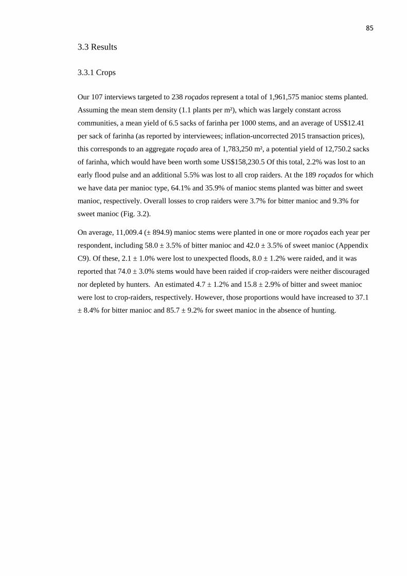
85

3.3 Results

3.3.1 Crops

Our 107 interviews targeted to 238 roçados represent a total of 1,961,575 manioc stems planted.

Assuming the mean stem density (1.1 plants per m²), which was largely constant across

communities, a mean yield of 6.5 sacks of farinha per 1000 stems, and an average of US$12.41

per sack of farinha (as reported by interviewees; inflation-uncorrected 2015 transaction prices),

this corresponds to an aggregate roçado area of 1,783,250 m², a potential yield of 12,750.2 sacks

of farinha, which would have been worth some US$158,230.5 Of this total, 2.2% was lost to an

early flood pulse and an additional 5.5% was lost to all crop raiders. At the 189 roçados for which

we have data per manioc type, 64.1% and 35.9% of manioc stems planted was bitter and sweet

manioc, respectively. Overall losses to crop raiders were 3.7% for bitter manioc and 9.3% for

sweet manioc (Fig. 3.2).

On average, 11,009.4 (± 894.9) manioc stems were planted in one or more roçados each year per

respondent, including 58.0 ± 3.5% of bitter manioc and 42.0 ± 3.5% of sweet manioc (Appendix

C9). Of these, 2.1 ± 1.0% were lost to unexpected floods, 8.0 ± 1.2% were raided, and it was

reported that 74.0 ± 3.0% stems would have been raided if crop-raiders were neither discouraged

nor depleted by hunters. An estimated 4.7 ± 1.2% and 15.8 ± 2.9% of bitter and sweet manioc

were lost to crop-raiders, respectively. However, those proportions would have increased to 37.1

± 8.4% for bitter manioc and 85.7 ± 9.2% for sweet manioc in the absence of hunting.

86

Figure 3.2. Summary number of manioc stems planted and lost per agricultural plot (roçado),

separated by type of manioc, on the basis of interview data. Dark green and dark red bars

respectively indicate the mean total number of manioc stems planted per roçado, and those that

would have been lost if crop raiders were not suppressed by hunting. Red bars indicate the number

of manioc stems actually lost to crop raiders, and blue bars indicate those lost to flooding (only

available for “All Manioc”). Vertical black lines represent standard errors.

87 Interviewees had resided in their respective communities for 20.1 ± 1.3 years. Mean journey time

to roçados from the community was 30.6 ± 2.8 minutes. Lethal methods to suppress crop raiders

included hunting (38.0% of all responses), using dogs (17.1%), traps (3.2%), and shooting (0.6%)

(Fig. 3.3). Nonlethal methods included tending the roçado and maintaining vigilance (12.0%),

using scarecrows (7.6%), firebreaks (7.0%), scaring animals away (4.4%), enclosing roçados with

nets (3.2%), maintaining the roçado weed-free (3.2%) and praying (0.6%). Only 2.5% reported

doing nothing to combat raiders, often because their roçado plot was too far away, and 0.6% that

their roçados did not succumb to crop raiders, thereby requiring no response.

Figure 3.3. Stacked bars summarising responses to categorical interview questions. Bar segment

height represents the percentage of responses or weighted responses. Bar1 = Ranked livelihood

activities. Green = agriculture. Blue = fishing. Gold = Welfare and PES payments. Purple =

extractivism. Grey = salaried work. Red = hunting. Black = other. Brown = timber. Orange

(imperceptible) = livestock. Bar2 = Ranked protein sources. Blue = caught wild fish. Red = hunted

game meat. Purple = equally important. Bar3 = “Have you killed animals in your roçados?” Red

= “yes”. Blue = “no”. Bar4 = Response to crop raiders. Red = lethal. Blue = nonlethal. Grey =

nothing. Black = crop raiders do not invade. Bar5 = method of transport to roçado. Brown = on

foot. Blue = un-motorised canoe. Grey = canoe with outboard motor.

88

3.3.2 Crop-raiders and other species

The prevalence of vertebrate species detected by camera traps or reported in interviews was

widely variable (Fig. 3.4). In total, 27 taxa were reported to enter roçados, especially caviomorph

rodents, cervids, tayasuids, armadillos, tapirs and felids. Ten of these species were reported to

raid crops, five of which (Dasyprocta fuliginosa, Pecari tajacu, Cuniculus paca, Mazama

americana and Echimyidae spp in order of importance) were rodents or ungulates representing

>99% of weighted crop raiding scores.

A total of 33 vertebrate taxa were reliably detected by camera traps, which yielded a shallower

rank-abundance curve than did interview data. The three most frequently detected species overall

(Dasyprocta fuliginosa, Mazama Americana and Cuniculus paca) were also frequently reported

crop raiders and were proportionally equally detected in either primary forest or successional

mosaics. Species frequently reported to enter roçados were also frequently detected by cameras

outside primary forest (Spearman’s Rho = 0.47; Fig. 3.5).

Nineteen taxa were frequently hunted, and these were often reported as crop raiders (p<0.001,

Spearman’s Rho = 0.41). The first (Tayassu pecari) and seventh (Tapirus terrestris) most

commonly reported hunted species, however, were infrequently camera-detected large-bodied

ungulates that were not reported as crop raiders. Seven taxa were reportedly killed at roçados, the

four top-ranking of which were also the four top-ranking crop raiders.

89

Figure 3.4: Species prevalence in interviews and camera detections. Values in Appendix A. i)

Stacked bar length represents species propensity to enter roçados as reported in interviews. Red =

considered a crop raider. Green = not considered a crop raider ii) Transparent black circles -

position along x axis represents standardised detection frequency per 100 CTN. Circle size

represents the degree to which the species was detected in primary forest iii) Empty blue circles –

position along x axis represents the percentage of weighted interview scores reporting the species

as hunted. Circle size represents the frequency of that species being reportedly killed in roçados

(larger = higher frequency).

90

Figure 3.5: Log₁₀ habitat selectivity index score and detection rate per species derived from camera

trap data. Larger circles indicate higher CTR. HSI Scores < 0 indicate the species had a higher

detection rate in primary forest. Colour represents taxonomic group as indicated in the legend.

3.3.3 Determinants of crop-raiding rates

Crop raider biomass detected by cameras increased with distance to the nearest town (Table 3.1).

In contrast, non-raider biomass was related to habitat type, with more pristine forest habitats

exhibiting higher biomass. GLMM models indicate that reported losses to crop raiders decreased

in heavily-settled areas. When modelled using GLMMHs, local human population density and

habitat score (a higher score representing less disturbed habitat) both negatively influenced the

chance of a roçado being raided, whereas human density alone negatively influenced the amount

lost to raiders.

91

Table 3.1. . Key predictors of the magnitude of manioc crop losses, crop-raider (and non-raider) biomass, and species composition sampled by camera-traps. Each row

represents a retained independent variable. For methodological details and variable derivation, see methods and Appendix C. Reference habitat is primary forest.

Model

number Data type

Dependent

variable Model type Model family

Retained independent

variable R²

Odds

ratio

Lower

confidence

interval

Upper

confidence

interval

P value

1 Interview Crop Losses GLMM Negative Binomial Local Human

Population NA 0.50 0.30 0.83 <0.01

2 Interview Crop Losses Hurdle - Zero Binomial Local Human

Population NA 0.35 0.22 0.56 <0.001

2 Interview Crop Losses Hurdle - Zero Binomial Habitat Intactness -

Score NA 0.72 0.52 0.99 <0.05

3 Interview Crop Losses Hurdle - Count Truncated QuasiPoisson Local Human

Population NA 0.74 0.55 1.00 >0.05 (0.053)

4 Camera trap Crop Raider

Biomass GLMM Negative Binomial

Distance to Nearest

City NA 1.34 1.02 1.76 <0.05

5 Camera trap Non-Raider

Biomass GLMM Negative Binomial

Habitat - Disturbed

Forest NA 0.58 0.20 1.68 >0.05

5 Camera trap Non-Raider

Biomass GLMM Negative Binomial Habitat - Capoeira NA 0.52 0.30 0.90 <0.05

5 Camera trap Non-Raider

Biomass GLMM Negative Binomial Habitat - Homestead NA 0.20 0.09 0.42 <0.001

6 Camera trap Species

Composition Permanova NA Habitat 0.07 NA NA NA <0.001

7 Camera trap Species

Composition Permanova NA

Habitat Intactness -

Deforestation 0.02 NA NA NA <0.01

92 NMDS ordination based on a Bray-Curtis distance matrix suggests that the species composition

of CT stations within successional mosaics represents a nested subset of species in primary forest

(Fig. 3.6). In ordination space, less disturbed forest habitat occupies the largest area, with more

disturbed habitats occupying small subsets, rather than a distinct space. Similarly, the main crop

raiding species are clustered in ordination space, whilst the larger number of non-raider species

are spread widely. Permanova analyses showed significant bivariate associations with habitat

category and primary forest conversion. Modest R² values indicate that the variables tested did

not explained much of the variation. The variable with the highest R² and lowest p value was

habitat category.

Figure 3.6. Ordination plots representing Bray Curtis distances from a matrix of standardised

camera trap data. Left panel – Circles and convex hulls represent habitat categories, where dark

green, blue, red and brown represent primary forest, disturbed forest, secondary forest and

homestead, respectively. Right panel – Number size and colour represent species propensity to

enter roçados and to crop raid, whereby larger number indicate a higher propensity to enter

roçados, black, grey and blue represent frequent crop raiders, infrequent crop raiders and non-

raiders, respectively. Species are numbered as followed. 1 = A. microtis, 2 = Crypturellus. Spp, 3

= C. paca, 4 = D. fuliginosa, 5 = Dasypus. Spp, 6 = D. marsupialis, 7 = Echimyidae. Spp, 8 = E.

barbara, 9 = L. pardalis, 10 = L. wiedii, 11 = Leptotilla. Spp, 12 = M. americana, 13 = M.

nemorivaga, 14 = Metachirus. Spp, 15 = M. tuberosum, 16 = M. pratii, 17 = M. tridactyla, 18 =

N. nasua, 19 = Odontophorus. Spp, 20 = O. guttata, 21 = P. onca, 22 = P. tajacu, 23 = P.

jacquacu, 24 = P. maximus, 25 = P. leucoptera, 26 = P. concolor, 27 = P. yagouaroundi, 28 = S.

iginitus, 29 = S. spadiceus, 30 = T. tetradactyla, 31 = T. terrestris, 32 = T. pecari, 33 = Tinamus.

Spp.

93

3.4 Discussion

3.4.1 The significance of losses to terrestrial vertebrate crop raiders

Terrestrial vertebrate crop raiding imposes a triple burden for semi-subsistence forest dwellers in

Amazonia. Firstly, although apparently modest, the overall mean reported losses to raiders of

5.5% are substantial, and mask large variability to the extent that some farmers every year are

ruined (c.f. Naughton‐Treves, 1998). Losses to crop raiders compound the hardship faced by

semi-subsistence farmers, whose livelihoods are additionally impacted by flooding. Secondly,

though sweet manioc is more palatable and requires less arduous processing (Frazer, 2010), the

nearly triple raiding rates associated with it, seemingly relegate it to a secondary horticulture

within roçados. Lastly and perhaps most importantly (Barua et al., 2013), farmers invest

substantial effort in protecting their fields, incurring attendant opportunity costs, and would suffer

nearly tenfold crop losses if they did not. The effects of guarding range from precluding

extremely high losses (Gillingham and Lee, 2003; Pérez and Pacheco, 2006) to largely ineffective

(Linkie et al., 2007). All anti-raider tactics along the Juruá, including setting nets, traps, hunting

with dogs, and creating scarecrows and firebreaks are labour-intensive, which is consistent with

other studies. For example Ugandan famers spend over 20% of their time guarding against crop

raiders in some months (Hill 2000), and Tanzanian farmers guard their fields on a full time basis

during high-risk months (Gillingham and Lee 2003).

More isolated farmers living in small communities far from towns experienced the highest losses

to crop raiders. This has been reported in other crop raiding studies (Hill, 2000; Naughton‐Treves

et al., 2003). These remote, low-density communities have the highest barriers to market and

lowest incomes (Parry et al., 2010), thereby suggesting a triple disadvantage in terms of their

socioeconomic welfare. Several urban respondents reported that past losses to crop raiders were

much higher. A respondent from a Carauari suburb reported that he “used to see cutias

(Dasyprocta fuliginosa) eating manioc five times in one day. Now there are not even tracks.” This

may reflect expanding urban populations with attendant increases in hunting pressure and

disturbance.

3.4.2 Hunting crop raiders

Potentially, hunting crop raiders around roçados is a ‘win-win’ strategy, reducing rates of raiding

and providing meat for local communities (Smith, 2005). Furthermore, as terrestrial vertebrate

crop raiders are often fecund, disturbance tolerant, and ubiquitous species, they are good

candidates for sustainable subsistence hunting.

Despite this, and in agreement with Naughton‐Treves et al., (2003), who found that on average,

crop losses to raiders were more valuable than hunting gains in terms of meat acquisition, we

94 found that hunting crop raiders may provide limited benefit to semi-subsistence agriculturalists in

our study area insofar as (1) nonlethal methods to suppress crop raiders were almost as commonly

reported as lethal methods; (2) Terrestrial game hunting in the Medio Juruá is secondary to fish as

a source of animal protein (Endo et al. 2016), and a modest livelihood component (Newton et al.,

2012), which is consistent with other studies of ribeirinho communities in lowland Amazonia

(Murrieta et al., 1999; Adams et al., 2009) and (3) the most hunted species, white-lipped peccary

(Tayassu pecari), is not considered a significant crop raider as its large herds rarely entered

roçado areas.

Notwithstanding this, Naughton‐Treves et al., (2003) encouragingly found that in remote areas

where hunting pressure has not greatly reduced large game abundance, hunting gains compensate

crop losses. This supports the notion that community location represents a livelihood trade-off

between access to natural resources and access to goods and services (Parry et al., 2010).

We also found that the most prolific crop raiding species were amongst the most commonly

hunted. The nineteen species reportedly hunted in our study accord with game offtake profiles

reported in other Neotropical studies (Redford and Robinson, 1987; Jerozolimski and Peres,

2003). Likewise, the species identified in our study as the most burdensome crop raiders were

also identified by Pérez and Pacheco (2006) and Naughton‐Treves et al., (2003). Tayassu pecari

is anomalous. Foraging in large herds and ranging over large areas (Peres, 1996; Fragoso, 1998),

this species is a stochastic boon for hunters and impossible to ignore even by those otherwise

disinclined to hunt. Although not regarded an important crop raider due to its infrequent

occurrence, several respondents commented that in the unfortunate event that a herd of Tayassu

pecari entered their roçado, the entire crop would be ruined.

Additionally, the nutritional benefit of meat may be disproportionate to the quantity consumed.

Indigenous Amazonian and to a lesser extent ribeirinho groups place extremely high nutritional

and cultural importance on game meat (Neel et al., 1964; Carneiro, 1970; Redford and Robinson,

1987).

Lastly, the key terms “hunting” and “livelihood”, were understood differently by respondents,

some of whom did not equate carrying a gun to their roçado and opportunistically killing animals

as hunting. They only considered hunting to be specifically setting out with the primary objective

of killing game. Similarly, some respondents did not consider strictly subsistence activities such

as hunting, even if those were frequently engaged in, to be a primary livelihood component. Thus

our interviews may underestimate the incidence and importance of opportunistic and subsistence

hunting.

95

3.4.3 Crop raiding species and the human landscape

Vertebrate species either reported to enter roçados or camera-trapped in their vicinities are a

small proportion of the assemblage detected by camera traps, and crop raiders are a smaller

proportion still. There are ecological, behavioural and demographic filters species must pass

through if they are to become burdensome raiders. The vast majority of Amazonian forest

vertebrates persist at low densities and are intolerant of highly disturbed habitats. Amongst the

most habitat-generalist, disturbance-tolerant species, only a small proportion are capable of

digging and ingesting manioc tubers or grazing their leaves, both of which are highly toxic to

generalist herbivores (Gleadow and Woodrow, 2002). This largely explains the much higher

crop-raiding rates observed for the more palatable sweet manic, which has a lower cyanide

content.

The zero hurdle model retained the habitat intactness score, implying that roçados surrounded by

more intact habitat were less likely to be raided. We anticipated the opposite effect, as

neighbouring undisturbed habitat acts as a reservoir for crop raiders. Other studies have shown

that crop raiding is strongly associated with areas near forest (Naughton‐Treves, 1998; Hill, 2000;

Linkie, 2007). This is an unexpected result that we treat with caution. Odds ratio confidence

intervals suggest that the relationship is weak. It may be that Neotropical crop raiders persist in

highly heterogeneous agricultural mosaics to a greater degree than anticipated. This is not the

case for non-raiders, whose biomass was markedly depressed in more disturbed habitats. A more

plausible explanation is the effect of landscape context. Unlike other crop-raiding study areas

throughout the tropics, the Medio Juruá region largely consists of vast tracts of contiguous

primary forest with deforestation and regrowth representing only ~1.8% of total area. At a

landscape scale, primary forest is thus not a limited habitat and habitat-generalist raiders may be

attracted to anthropogenic resources.

Though anthropogenic factors such as community size and proximity to urban centers had a

negative effect on crop raiding, household distance to roçado did not. This is counterintuitive as

roçados farther removed from the centre of the community are expected to experience less

hunting pressure and vigilance. Whilst we can conclude that anthropogenic pressure in general

influences crop raiders, we cannot confirm that this effect is spatially concentrated.

3.4.4 A forest ecosystem disservice?

Crop raiding can be considered an ecosystem disservice. Anthropogenic pressures negatively

influence rates of crop raiding, so that Amazonian communities sometimes pay a high price for

living at low densities in a high species-richness, intact environment. The biodiverse ecosystem

per se may not be at fault. Crop raiding species tolerate human disturbance, and even much

simplified ecosystems include them. Indeed, biotic disturbance and simplification may exacerbate

96 levels of crop raiding and pests (Andow, 1983; Yamada and Muroyama, 2010). Furthermore,

camera trap and interview data suggest that crop raiders are closely attended by their natural

predators in faunally-intact vertebrate assemblages such as those along the Juruá, presumably

buffering raiding rates. However, this is inadequate consolation to local villagers who may also

incur significant losses to forest carnivores. Predators of large forest rodents (dasyproctids and

echimyids), such as ocelots and tayras, are frequently implicated in livestock depredation. Large

predators of ungulates (e.g. Mazama americana and Pecari tajacu) such as large felids (Panthera

onca and Puma concolor), are feared killers of domestic pigs and cattle and occasionally people

(Conforti, and de Azevedo, 2003; Soto-Shoender, and Giuliano, 2011).

3.4.5 Dog hunting

Amongst the strategies to reduce crop raiding, 17.1% of responses reported hunting with dogs, or

using dogs to scare away raiders. This is a contentious issue. Dogs are believed to drastically

impact local fauna (Galetti and Sazima, 2006), covering long distances, killing small game,

maiming and chasing away larger animals and causing additional disturbance through their noise

and scent. There have been calls to enforce bans on the use of dogs as a hunting tool in Brazil

(Cunha and De Almeida, 2000; Carvalho and Pezzuti, 2010). Their common use suggests that as

a tool for reducing rates of crop raiding, however, dogs have merit. One interviewee reported that

their community suffered high consistent losses to collared peccary herds, until they employed a

professional hunter with dogs from a nearby community to kill and scare them away. The

intervention was so effective that they later acquired hunting dogs of their own.

3.4.6 Interview reliability

Our interview data likely suffers from social desirability bias (John et al., 2010). Our interviews

included potentially sensitive topics such as livelihoods and hunting. Techniques to increase the

reliability of responses to sensitive questions (randomised response techniques (RRT) or similar)

were not used. Interviews were carried out by non-locals, who may be perceived as outsiders. We

asked respondents to remember and quantify losses to crop raiders and to estimate counterfactual

losses in the absence of crop protection. Plausibly, respondents may have been motivated to over-

report losses and under-report hunting. This is because hunting may be perceived to be an activity

that researchers disapprove of, whilst high crop losses not only highlight livelihood challenges,

but justify hunting.

Nonetheless, we argue that our data are trustworthy. Our research group has been active in the

Medio Jurua region since 2007 and has built trust through involvement in popular and successful

resource management programs such as pirarucu (Arapaima spp) fisheries. Interviewers built

trust by acting respectfully towards local communities (see Appendix C.10). We asked potentially

sensitive questions in a direct manner, trusting the respondents rather than employing RRT.

97 The consistency of our interview results both with comparable existing studies (Naughton-Treves,

1998; Hill, 2000; Nchanji 2002) and with our camera data, increases our confidence in them. A

coherent picture emerges due to the complementarity between camera trap and interview data,

suggesting that the data are broadly reliable. Species frequently detected by cameras, especially in

disturbed habitats, were those reported to frequent roçados. Likewise, nearby human population

density (as quantified by community size or proximity to city), was associated with both lower

reported crop losses and with lower detected crop raider biomass. By contrast habitat disturbance

(measured by habitat type or amount of nearby deforestation), was associated with lower non-

raider biomass and simplified species composition. Given the complementary strengths and

weaknesses of these two data collection methods, we suggest that mixed methods hold promise

for understanding socio-ecological problems.

3.5 Conclusions

Terrestrial vertebrate crop raiding represents a burdensome ecosystem disservice for rural

Amazonians, who invest substantial amounts of time energy in protecting crops to avoid

significant losses. Crop raiding is heightened in sparsely settled areas, thereby compounding the

economic hardship faced by small communities that are already disadvantaged by isolation from

the material, service and information economy of urban centres. Crop raiders comprise a select

group of habitat-generalist, disturbance-tolerant and relatively fecund species, which apparently

make them ideal candidates for sustainable subsistence hunting. However, local semi-subsistence

communities consider high crop raider biomass to be a livelihood threat, rather than a hunting

opportunity.

98

3.6 References

Adams, C., Murrieta, R., Siqueira, A., Neves, W. and Sanches, R., 2009. Bread of the

land: the invisibility of manioc in the Amazon. In Amazon Peasant Societies in a Changing

Environment (pp. 281-305). Springer Netherlands.

Alvard, M.S., Robinson, J.G., Redford, K.H. and Kaplan, H., 1997. The sustainability of

subsistence hunting in the Neotropics. Conservation Biology, 11(4), pp.977-982.

Anderson, M.J., 2001. A new method for non‐parametric multivariate analysis of

variance. Austral Ecology, 26(1), pp.32-46.

Andow, D., 1983. The extent of monoculture and its effects on insect pest populations

with particular reference to wheat and cotton. Agriculture, Ecosystems & Environment, 9(1),

pp.25-35.

Balmford, A. and Whitten, T., 2003. Who should pay for tropical conservation, and how

could the costs be met? Oryx, 37(02), pp.238-250.

Baptista, L.F., Trail, P.W. and Horblit, H.M., 1997. Family Columbidae (pigeons and

doves). In: del Hoyo, J.; Elliott, A. & Sargatal, J. (eds): Handbook of birds of the world, Volume

4: pp.60-243 Sandgrouse to Cuckoos. Lynx Edicions, Barcelona

Barlow, J., Gardner, T.A., Araujo, I.S., Ávila-Pires, T.C., Bonaldo, A.B., Costa, J.E.,

Esposito, M.C., Ferreira, L.V., Hawes, J., Hernandez, M.I. and Hoogmoed, M.S., 2007.

Quantifying the biodiversity value of tropical primary, secondary, and plantation

forests. Proceedings of the National Academy of Sciences, 104(47), pp.18555-18560.

Barua, M., Bhagwat, S.A. and Jadhav, S., 2013. The hidden dimensions of human–

wildlife conflict: health impacts, opportunity and transaction costs. Biological Conservation, 157,

pp.309-316.

Benchimol, M. and Peres, C.A., 2015. Widespread forest vertebrate extinctions induced

by a mega hydroelectric dam in lowland Amazonia. PloS One, 10(7), p.e0129818.

Bolker BM., 2012. glmmADMB: Generalized Linear Mixed Models Using AD Model

Builder. R package version 0.7. 2.1. 2012

Brasil, I.N.P.E., 2009. Projeto PRODES: Monitoramento da Floresta Amazônica

Brasileira por Satélite. Instituto Nacional de Pesquisas Espaciais (INPE), São José dos Campos,

São Paulo, Brasil. Disponível em< http://www. obt. inpe. br/prodes.

Brechin, S.R., Wilshusen, P.R., Fortwangler, C.L. and West, P.C., 2002. Beyond the

square wheel: toward a more comprehensive understanding of biodiversity conservation as social

and political process. Society & Natural Resources, 15(1), pp.41-64.

99

Carboneras, C., 1992. Family Anatidae (ducks, geese and swans).Handbook of the Birds

of the World, 1, pp.536-628. In: del Hoyo, Josep; Elliott, Andrew & Sargatal, Jordi

(eds.): Handbook of Birds of the World (Volume 1: Ostrich to Ducks): 536–629. Lynx Edicions,

Barcelona

Carneiro, R.L., 1970. Hunting and hunting magic among the Amahuaca of the Peruvian

Montaña. Ethnology, 9(4), pp.331-341.

Carvalho, E.A. and Pezzuti, J.C., 2010. Hunting of jaguars and pumas in the Tapajós–

Arapiuns Extractive Reserve, Brazilian Amazonia. Oryx, 44(04), pp.610-612.

Clarke, K.R. and Warwick, R.M., 2001. Change in Marine Communities: An Approach

to Statistical Analysis and Interpretation, (Second Edition). Primer-E Ltd: Plymouth, UK

Cock, J.H., 1982. Cassava: a basic energy source in the tropics. Science, 218(4574),

pp.755-762.

Conforti, V.A. and de Azevedo, F.C.C., 2003. Local perceptions of jaguars (Panthera

onca) and pumas (Puma concolor) in the Iguacu National Park area, south Brazil. Biological

Conservation, 111(2), pp.215-221.

Coomes, O.T., Grimard, F. and Burt, G.J., 2000. Tropical forests and shifting cultivation:

secondary forest fallow dynamics among traditional farmers of the Peruvian Amazon. Ecological

Economics, 32(1), pp.109-124.

Cunha, M.C.D. and De Almeida, M.W., 2000. Indigenous people, traditional people, and

conservation in the Amazon. Daedalus, 129(2), pp.315-338.

Dunning Jr, J.B. ed., 1992. CRC handbook of avian body masses. CRC press, Florida,

USA

Emmons, L.H. and Feer, F., 1997. Neotropical rainforest mammals. A field

guide, (Second edition.) University of Chicago Press, Chicago, Illinois

Estrada, A., 2006. Human and non-human primate co-existence in the Neotropics: a

preliminary view of some agricultural practices as a complement for primate conservation.

Ecological and Environmental Anthropology (University of Georgia). Paper 3.

Fearnside, P.M., 1989. Extractive reserves in Brazilian Amazonia. Bioscience, 39(6),

pp.387-393.

Fragoso, J., 1998. Home Range and Movement Patterns of White‐lipped Peccary

(Tayassu pecari) Herds in the Northern Brazilian Amazon1.Biotropica, 30(3), pp.458-469.

Fraser, J.A., 2010. The diversity of bitter manioc (Manihot esculenta Crantz) cultivation

in a whitewater Amazonian landscape. Diversity, 2(4), pp.586-609.

100

Galetti, M. and Sazima, I., 2006. Impact of feral dogs in an urban Atlantic forest fragment

in southeastern Brazil. Natureza e Conservação, 4(1), pp.146-151.

Gaston, K.J., 2000. Global patterns in biodiversity. Nature, 405(6783), pp.220-227.

Gavin, M.C., 2007. Foraging in the fallows: Hunting patterns across a successional

continuum in the Peruvian Amazon. Biological Conservation, 134(1), pp.64-72.

Gavin, M.C., Solomon, J.N. and Blank, S.G., 2010. Measuring and monitoring illegal use

of natural resources. Conservation Biology, 24(1), pp.89-100.

Gillingham, S. and Lee, P.C., 2003. People and protected areas: a study of local

perceptions of wildlife crop-damage conflict in an area bordering the Selous Game Reserve,

Tanzania. Oryx, 37(03), pp.316-325.

Gleadow, R.M. and Woodrow, I.E., 2002. Mini-Review: constraints on effectiveness of

cyanogenic glycosides in herbivore defense. Journal of Chemical Ecology, 28(7), pp.1301-1313.

Hansen, M.C., Potapov, P.V., Moore, R., Hancher, M., Turubanova, S.A., Tyukavina, A.,

Thau, D., Stehman, S.V., Goetz, S.J., Loveland, T.R. and Kommareddy, A., 2013. High-

resolution global maps of 21st-century forest cover change. Science, 342(6160), pp.850-853.

Hartter, J., Ryan, S.J., Southworth, J. and Chapman, C.A., 2010. Fortresses and

fragments: impacts of fragmentation in a forest park landscape. In Proceedings of IUFRO

Landscape Ecology International Conference. Braganca: Portugal.

Haugaasen, T. and Peres, C.A., 2005. Mammal assemblage structure in Amazonian

flooded and unflooded forests. Journal of Tropical Ecology, 21(02), pp.133-145.

Hill, C.M., 2000. Conflict of interest between people and baboons: crop raiding in

Uganda. International Journal of Primatology, 21(2), pp.299-315.

IBGE, 2007. Censo Demografico 2007. Instituto Brasileiro de Geographia e Estatistica.

Jerozolimski, A. and Peres, C.A., 2003. Bringing home the biggest bacon: a cross-site

analysis of the structure of hunter-kill profiles in Neotropical forests. Biological

Conservation, 111(3), pp.415-425.

John, F.A.S., Edwards-Jones, G., Gibbons, J.M. and Jones, J.P., 2010. Testing novel

methods for assessing rule breaking in conservation. Biological Conservation, 143(4), pp.1025-

1030.

Junk, W.J., 1984. Ecology of the várzea, floodplain of Amazonian whitewater rivers.

In The Amazon (pp. 215-243). Springer Netherlands.

101

Krief, S., Cibot, M., Bortolamiol, S., Seguya, A., Krief, J.M. and Masi, S., 2014. Wild

chimpanzees on the edge: nocturnal activities in croplands. PloS One, 9(10), p.e109925.

Linkie, M., Dinata, Y., Nofrianto, A. and Leader‐Williams, N., 2007. Patterns and

perceptions of wildlife crop raiding in and around Kerinci Seblat National Park, Sumatra. Animal

Conservation, 10(1), pp.127-135.

Mackenzie, C.A. and Ahabyona, P., 2012. Elephants in the garden: Financial and social

costs of crop raiding. Ecological Economics, 75, pp.72-82.

Mittermeier, R.A., Myers, N., Thomsen, J.B., Da Fonseca, G.A. and Olivieri, S., 1998.

Biodiversity hotspots and major tropical wilderness areas: approaches to setting conservation

priorities. Conservation Biology, 12(3), pp.516-520.

Montagnac, J.A., Davis, C.R. and Tanumihardjo, S.A., 2009. Nutritional value of cassava

for use as a staple food and recent advances for improvement. Comprehensive Reviews in Food

Science and Food Safety, 8(3), pp.181-194.

Murrieta, R.S.S., Dufour, D.L. and Siqueira, A.D., 1999. Food consumption and

subsistence in three caboclo populations on Marajó Island, Amazonia, Brazil. Human

Ecology, 27(3), pp.455-475.

Naughton‐Treves, L., 1998. Predicting patterns of crop damage by wildlife around Kibale

National Park, Uganda. Conservation Biology, 12(1), pp.156-168.

Naughton‐Treves, L., Mena, J.L., Treves, A., Alvarez, N. and Radeloff, V.C., 2003.

Wildlife Survival Beyond Park Boundaries: the Impact of Slash‐and‐Burn Agriculture and

Hunting on Mammals in Tambopata, Peru. Conservation Biology, 17(4), pp.1106-1117.

Nchanji, A., 2002. Crop damage around northern Banyang-MBO wildlife sanctuary. In:

Hill, C.M., Osborn, V., Plumptre, A.J. (Eds.), Human–Wildlife Conflict: Identifying the Problem

and Possible Solutions. Albertine Rift Technical Report Series, vol. 1. Wildlife Conservation

Society, Bronx, NY, pp. 68–78.

Neel, J.V., Salzano, F.M., Junqueira, P.C., Keiter, F. and Maybury-Lewis, D., 1964.

Studies on the Xavante Indians of the Brazilian Mato Grosso. American Journal of Human

Genetics, 16(1), p.52.

Newton, P., Endo, W. and Peres, C.A., 2012. Determinants of livelihood strategy

variation in two extractive reserves in Amazonian flooded and unflooded forests. Environmental

Conservation, 39(02), pp.97-110.

Niedballa, J., Courtiol, A., Sollmann, R., Mathai, J., Wong, S.T., Nguyen, A.T.T.,

Mohamed, A.B., Tilker, A., Wilting, A. camtrapR Package. R package version 0.99.0. 2016.

102

Nowak, R.M., 1999. Walker's mammals of the world (Vol. 1). JHU Press.

Nyhus, P.J. and Sumianto, R.T., 2000. Crop‐raiding elephants and conservation

implications at Way Kambas National Park, Sumatra, Indonesia. Oryx, 34(4), pp.262-274.

Oksanen, J., Blanchet, F.G., Kindt, R., Legendre, P., Minchin, P.R., O’Hara, R.B.,

Simpson, G.L., Solymos, P., Stevens, M.H.H. and Wagner, H., 2015. Vegan: Community

Ecology Package. R package version 2.0-10. 2013.

Parry, L. and Peres, C., 2015. Evaluating the use of local ecological knowledge to

monitor hunted tropical forest wildlife over large spatial scales. Ecology and Society, 20(3).

Parry, L., Barlow, J. and Peres, C.A., 2009. Allocation of hunting effort by Amazonian

smallholders: implications for conserving wildlife in mixed-use landscapes. Biological

Conservation, 142(8), pp.1777-1786.

Parry, L., Day, B., Amaral, S. and Peres, C.A., 2010. Drivers of rural exodus from

Amazonian headwaters. Population and Environment, 32(2-3), pp.137-176.

Peres, C.A., 1996. Population status of white-lipped Tayassu pecari and collared

peccaries T. tajacu in hunted and unhunted Amazonian forests. Biological Conservation, 77(2),

pp.115-123.

Peres, C.A., 1997. Effects of habitat quality and hunting pressure on arboreal folivore

densities in Neotropical forests: a case study of howler monkeys (Alouatta spp.). Folia

Primatologica, 68(3-5), pp.199-222.

Pérez, E. and Pacheco, L.F., 2006. Damage by large mammals to subsistence crops

within a protected area in a montane forest of Bolivia. Crop Protection, 25(9), pp.933-939.

Peroni, N., Kageyama, P.Y. and Begossi, A., 2007. Molecular differentiation, diversity,

and folk classification of “sweet” and “bitter” cassava (Manihot esculenta) in Caiçara and

Caboclo management systems (Brazil). Genetic Resources and Crop Evolution, 54(6), pp.1333-

1349.

Picmeta Systems, [Computer software]. 2016. Picture Information Extractor. Retrieved

from http://www.picmeta.com/products/picture-information-extractor.htm

Pienkowski, M.W., Watkinson, A.R., Kerby, G., Naughton‐Treves, L., Treves, A.,

Chapman, C. and Wrangham, R., 1998. Temporal patterns of crop‐raiding by primates: linking

food availability in croplands and adjacent forest. Journal of Applied Ecology, 35(4), pp.596-606.

Redford, K.H. and Robinson, J.G., 1987. The game of choice: patterns of Indian and

colonist hunting in the Neotropics. American Anthropologist, 89(3), pp.650-667.

103

Rowcliffe, J.M. and Carbone, C., 2008. Surveys using camera traps: are we looking to a

brighter future? Animal Conservation, 11(3), pp.185-186.

Sachs, J.D., Mellinger, A.D. and Gallup, J.L., 2001. The geography of poverty and

wealth. Scientific American, 284(3), pp.70-75.Gaston, K.J., 2000. Global patterns in

biodiversity. Nature, 405(6783), pp.220-227.

Smith, D.A., 2005. Garden game: shifting cultivation, indigenous hunting and wildlife

ecology in Western Panama. Human Ecology, 33(4), pp.505-537.

Smith, D.A., 2008. The spatial patterns of indigenous wildlife use in western Panama:

implications for conservation management. Biological Conservation, 141(4), pp.925-937.

Sollmann, R., Mohamed, A., Samejima, H. and Wilting, A., 2013. Risky business or

simple solution–Relative abundance indices from camera-trapping. Biological Conservation, 159,

pp.405-412.

Soto-Shoender, J.R. and Giuliano, W.M., 2011. Predation on livestock by large

carnivores in the tropical lowlands of Guatemala. Oryx, 45(04), pp.561-568.

Sukumar, R., 1990. Ecology of the Asian elephant in southern India. II. Feeding habits

and crop raiding patterns. Journal of Tropical Ecology, 6(01), pp.33-53.

Tourangeau, R. and Smith, T.W., 1996. Asking sensitive questions the impact of data

collection mode, question format, and question context. Public Opinion Quarterly, 60(2), pp.275-

304.

Unruh, J.D., 1988. Ecological aspects of site recovery under swidden-fallow management

in the Peruvian Amazon. Agroforestry Systems, 7(2), pp.161-184.

Veloso, H.P., 1982. Fitogeografia brasileira: classificação fisionômico-ecológica da

vegetação Neotropical. RADAMBRASIL.

Wang, S.W., Curtis, P.D. and Lassoie, J.P., 2006. Farmer perceptions of crop damage by

wildlife in Jigme Singye Wangchuck National Park, Bhutan. Wildlife Society Bulletin, 34(2),

pp.359-365.

Winterhalder, B. and Lu, F., 1997. A forager‐resource population ecology model and

implications for indigenous conservation. Conservation Biology, 11(6), pp.1354-1364.

Yamada, A. and Muroyama, Y., 2010. Effects of vegetation type on habitat use by crop-

raiding Japanese macaques during a food-scarce season. Primates, 51(2), pp.159-166.

Zhang, W., Ricketts, T.H., Kremen, C., Carney, K. and Swinton, S.M., 2007. Ecosystem

services and dis-services to agriculture. Ecological Economics, 64(2), pp.253-260.

104

APPENDIX A

Table B1

Summarised camera trap, interview and trait data per species. Camera trap data do not distinguish between small armadillos. NA indicates species not reliably

detected by camera traps or habitat selectivity index cannot be calculated because camera detections are zero. CTR = Detections per 100CT Nights (all habitats). HSI

= Habitat Selectivity Index. Interview data are percentages of summed weighted scores. Body Mass sources a = Baptista et al., 1997, b = Dunning, 1992, c = Emmons

and Feer, 1997, d = Carboneras, 1992, e = Nowak, 1999, f = Peres (unpublished). Where male and female adult biomass for a given species differ, the mean was used.

Where only a range of adult biomass was known for a given species, the mean of the upper and lower limits was used.

Binomial

/Designation Taxa English Name CTR HSI Hunted

Killed

in

Roçados

Enters

Roçados:

Crop

Raider

Enters

Roçados:

Non-

Raider

Body

Mass,

g

Source

All Cingulata

small Xenarthra

Small Armadillos

All 1.4 -0.44 2.73 0 0.14 9.17 4800 c

Alouatta spp Primates Howler Monkey NA NA 4.03 0 0 0 6500 f

Atelocynus

microtis

Carnivores

Other Short-Eared Dog 0.24 -2.05 0 0 0 0 7750 c

Cabassous

unicinctus Xenarthra

Southern Naked

Tailed Armadillo NA NA 0 0 0.04 0.23 3200 c

Cairina moschata Birds Muscovy Duck 0 NA 0.37 1 0.1 0 2550 d

Callicebus spp Primates Titi Monkey NA NA 0 0 0 0.07 1125 f

Cebus albifrons Primates

White Fronted

Capuchin

Monkey

NA NA 0 0 0 0.14 2700 f

Crypturellus spp Birds Tinamou Small 0.83 -0.64 2.35 1 0.07 1.1 420 f

Cuniculus paca Rodents Paca 4.92 -0.04 14.36 12 12.74 0.58 9500 f

Dasyprocta

fuliginosa Rodents Agouti 6.99 -0.07 8.01 53 23.02 0.29 4500 f

Dasypus kappleri Xenarthra Greater Long-

Nosed Armadillo NA NA 0 0 0.04 1.96 10150 c

105

Binomial

/Designation Taxa English Name CTR HSI Hunted

Killed

in

Roçados

Enters

Roçados:

Crop

Raider

Enters

Roçados:

Non-

Raider

Body

Mass,

g

Source

Didelphis

marsupialis Marsupials

Common

Opossum 1.19 0.09 0 0 0 0 1088 c

Echimyidae spp Rodents Spiny Rat 1.02 -0.75 0 0 0.84 0 560 c

Eira barbara Carnivores

Other Tayra 0.86 -0.83 0 0 0 1.35 4850 c

Hydrochoerus

hydrochaeris Rodents Capybara 0 NA 0.41 0 0 0.29 50000 c

Lagothrix spp Primates Woolly Monkey NA NA 1.31 0 0 0 8710 f

Leopardus

pardalis Felids Ocelot 1.21 0.04 0 0 0 0.09 15000 f

Leopardus wiedii Felids Margay 0.1 -1.43 0 0 0 0.52 6000 c

Leptotila spp Birds White Tipped

Dove 0.64 -1.42 0 0 0.07 1.67 149 a

Mazama

americana Ungulates Red Brocket Deer 6.57 0.34 8.22 6 3.77 15.63 30000 f

Mazama

nemorivaga Ungulates

Grey Brocket

Deer 0.89 -0.96 1.25 0 0 0 18000 f

Metachirus spp Marsupials Brown Four-Eyed

Opossum 0.52 -0.57 0 0 0 0 390 c

Mitu tuberosum Birds Razor-Billed

Curassow 2.23 -0.1 8.21 0 0.07 2.22 3000 f

Myoprocta pratti Rodents Green Acouchi 0.78 -0.9 0 1 0 0.14 750 f

Myrmecophaga

tridactyla Xenarthra Giant Anteater 0.76 -0.27 0 0 0 0.48 30500 c

Nasua nasua Carnivores

Other Coati 0.14 -1.83 0 0 0 0 5100 c

Neochen jubata Birds Orinoco Goose 0 NA 0.13 0 0 0 1396 d

Odontophorus

spp Birds Wood Quail 0.07 -1.54 0 0 0 0 310 f

106

Binomial

/Designation Taxa English Name CTR HSI Hunted

Killed

in

Roçados

Enters

Roçados:

Crop

Raider

Enters

Roçados:

Non-

Raider

Body

Mass,

g

Source

Panthera onca Felids Jaguar 0.17 -0.79 0.15 0 0 1.7 80000 f

Pecari tajacu Ungulates Collared Peccary 1.07 0.09 17 25 15.89 0 25000 f

Penelope

jacquacu Birds Spix's Guan 0.19 -0.86 0.32 0 0 0.08 1280 f

Priodontes

maximus Xenarthra Giant Armadillo 0.14 -0.34 0 0 0 1.59 30000 c

Psophia

leucoptera Birds

Pale Winged

Trumpeter 1.88 -1.31 0 0 0 0 1200 f

Puma concolor Felids Puma 0.48 0.04 0.15 0 0 1.17 45000 c

Puma

yagouaroundi Felids Jaguarundi 0.1 -1.43 0 0 0 0 8000 f

Saimiri sciureus Primates Squirrel Monkey NA NA 0 0 0 0.1 940 f

Sciurus ignitus Rodents Bolivian Squirrel 0.12 1.68 0 0 0 0 700 f

Sciurus

spadiceus Rodents

Southern Amazon

Red Squirrel 0.54 -0.74 0 0 0 0 1200 f

Tamandua

tetradactyla Xenarthra

Southern

Tamandua 0.17 -1.9 0 0 0 0 4500 c

Tapirus terrestris Ungulates Tapir 0.02 -1.09 5.5 0 0 3.09 16000

0 f

Tayassu pecari Ungulates White Lipped

Peccary 0.05 -0.05 20.74 0 0 0.19 32000 f

Tinamus spp Birds Tinamou Large 0.57 -1.07 4.75 1 0.07 1.1 1200 f

Tolypeutes spp Xenarthra Three Banded

Armadillo NA NA 0 0 0.04 1.96 1300 e

107

Table B2

Summary Camera Trap Data

Metric Units Mean N Standard

Deviation

Standard

Error

Sum

Total

Camera Deployment Duration Camera trap nights 31.87 132 5.64 0.49 4206.21

Distance to Nearest Camera m 974.40 132 1997.86 173.89 NA

Biomass of Crop Raiders Detected kg 96.47 132 128.38 11.17 12734.05

Biomass of Non-Raiders Detected kg 41.54 132 51.27 4.46 5483.80

Wild Species Richness N species 4.80 132 3.40 0.30 32.00

N Detections 11.75 132 11.95 1.04 1551.00

Diversity Shannon Index Reciprocal 3.27 132 2.08 0.18 NA

Várzea Within 500m of camera m² 232132.89 132 284243.71 24740.24 NA

Deforestation Within 500m of camera m² 218736.14 132 185650.32 16158.79 NA

Households Within 4km (travel distance) of camera N households 16.77 132 16.70 1.45 NA

Fluvial Distance to Nearest City m 132161.75 132 61403.25 5344.47 NA

Population of Nearest City N households 3310.45 132 1422.25 123.79 NA

108

Supplementary Figure 3.1. Scatter plots of interview and camera data per species. Linear

regression lines (red) and lowess lines (blue). Left – The relationship between a species

propensity to enter roçados as reported in interviews, and the camera trap rate outside of

primary forest. p<0.001, adjusted R²= 0.73. Spearman’s Rho = 0.47. Right – The relationship

between a species propensity to crop raid as reported in interviews, and its importance as a

hunted species as reported in interviews. p<0.001, adjusted R² = 0.32. Spearman’s Rho = 0.41.

109

APPENDIX B

Interview Script

110

111

112

Appendix C - Methodological Details

1. For camera trap deployments, Bushnell Trophy-Cam, Trophy-Cam HD, and Reconyx

HC500 Hyperfire models were used. Camera sensors were set to high sensitivity. They

took 3 sequential burst photographs or 3 second video clips. A red light flash was used in

very low light. Only deployments close (1.8km) to the agricultural mosaic were used for

the analysis. Deployments were not made in várzea. Deployments outside contiguous

primary forest were 25m from the habitat edge to control for edge effects. When

deploying cameras, a community resident was employed to aid in the identification of

suitable locations and determine the age of capoeiras since abandonment. Locations were

not chosen to deliberately maximise detection (for example beneath fruiting trees), but

conspicuous obstacles to detection were avoided. Bait was not used. Locations were

chosen to have relatively flat ground, relatively unobscured by large trees/obstacles. Thin

vegetation was cleared in a cone of 7 paces long by 7 paces wide in-front of the camera to

permit detection and avoid detecting the movement of vegetation. Cameras were deployed

at knee height, attached to trees. Walk-tests were performed to confirm correct

positioning. Mothballs and tampons were put inside cameras along with batteries to repel

insects and protect against humidity. A GPS waypoint was always taken. When cameras

were removed, a note was made of any problems or malfunctions such as water ingress,

insect attack, dislodgement or battery failure.

2. When summarising interview data, where single numeric responses were given, means

were calculated. Where multiple unranked categorical responses were given, the number

of responses per category were summed. Where multiple ranked categorical responses

were given, a summed, rank-weighted score per category was calculated (∑ (∑ (ranked1)

+ ∑ (ranked2/2) + ∑ (ranked3/3)…)).

3. Várzea and habitat disturbance. For camera deployments, INPE PRODES, 2009, Hansen

et al., (2013) Global Forest Change (GFC) datasets were combined because though the

GFC data is 30m rather than 120m pixel resolution and extends to 2014, it does not

account for deforestation that occurred before 2000. Cells were reclassified into either

deforested or not deforested. For GFC data, 50% deforested was used as the cut off.

Deforested pixels were converted to polygons and merged. 500m was considered

appropriate given the heterogeneous and fine-scale nature of the agricultural mosaics.

4. Distance-weighted variables for várzea, deforestation and local human population were

calculated, but as these were not found to improve models, they were excluded from

further analysis. Deforestation and várzea, polygons were separately converted to raster

grid cells of 30m resolution to match the GFL dataset. The centre of each pixel was

converted to a point. The distance from each camera to each point was calculated. This

113

was linear distance in the case of várzea and deforestation and transport distance in the

case of households. Three weighted scores were calculated a) ∑ (1/distance) b) ∑

(1/(square root(distance))) c) ∑ (1/(natural log(distance))).

5. Respondents were asked what land use/land cover (from now “land cover”) bordered each

of their roçados. Respondents were allowed up to four responses. Each land cover type

was assigned a score (see table below) reflecting the degree of disturbance, with 10

indicating low disturbance contiguous primary forest and 1 indicating high disturbance

homestead. Likewise, a várzea score was assigned, 1 indicating várzea and 0 indicating

non-várzea. Scores per roçado were summed and divided by the number of responses, to

give the mean “intactness” and “várzea” of the land cover surrounding the roçado.

Portuguese land cover/

land use description English Equivalent

Intactness

Score

Várzea

Score

terra firme primary forest unflooded 10 0

várzea primary forest seasonally flooded 10 1

mata secundaria secondary forest 8 0

capoeira velha old abandoned roçado 6 0

capoeira nova newly abandoned roçado 4 0

açaí acai palm (Euterpe oleracea) plantation 3 0

pupunha peach-palm (Bactris gasipaes) plantation 3 0

roçado agricultural field 2 0

pasto pasture 2 0

campo field (for cattle or football) 2 0

comunidade community 1 0

6. Data validation of households and deforestation. The table below compares the PRODES

raster datasets between 2007 and 2013. The 2009 dataset was chosen because it has the

smallest area of cloud and no-data and the largest area of data. It also corresponds closely

in time to the 2007-2009 households census. The rural households points shapefile was

aggregated at the level of census sector and district for the states of Amazonas, Para, Acre,

Mato Grosso, Rondônia and Roraima, so that it could be compared to the IBGE 2007 rural

population count. Similarly, the 2009 PRODES deforestation data was compared to the

Hansen et al Global Forest Loss (GFL) dataset. The GFL “Year of gross forest cover loss

event” raster layer was used so that loss until 2009 could be compared. In both cases, cells

were reclassified into either deforested or not deforested. A subset of data for which there

was both PRODES and GFL data was taken from the 00N_070W degree granule in the

state of Amazonas. The data were aligned and aggregated (using ArcGIS tools “extract by

mask” and “aggregate”) to a cell size of roughly 12500m, representing a 100 cell factor

aggregation of the PRODES dataset. A 30km buffer was erased from this area to exclude

edge effects caused by raster aggregation, leaving an area of analysis of 1,072,620 km².

For both deforestation and households, a Spearman’s rank test was performed. The rural

households point shapefile and the IBGE 2007 rural population census, were found to be

strongly correlated. Aggregated by census sector, N = 8314, spearman value 0.69.

Aggregated by district, N= 721, spearman value, 0.85. Likewise, the 2009 PRODES

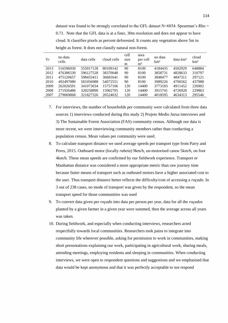
114

dataset was found to be strongly correlated to the GFL dataset N=6854. Spearman’s Rho =

0.71. Note that the GFL data is at a finer, 30m resolution and does not appear to have

cloud. It classifies pixels as percent deforested. It counts any vegetation above 5m in

height as forest. It does not classify natural non-forest.

Yr no data

cells data cells cloud cells

cell

size

m

area

per cell

m²

no data

km² data km²

cloud

km²

2013 516596930 555917128 80109142 90 8100 4184435 4502929 648884

2012 476386530 596127528 38370048 90 8100 3858731 4828633 310797

2011 475120657 598433411 36681641 90 8100 3848477 4847311 297121

2010 492497080 581056988 54072551 90 8100 3989226 4706562 437988

2009 262026591 341073034 15757106 120 14400 3773183 4911452 226902

2008 271926486 328258890 15962705 120 14400 3915741 4726928 229863

2007 279069068 321827326 20524032 120 14400 4018595 4634313 295546

7. For interviews, the number of households per community were calculated from three data

sources 1) interviews conducted during this study 2) Projeto Medio Jurua interviews and

3) The Sustainable Forest Association (FAS) community census. Although our data is

more recent, we were interviewing community members rather than conducting a

population census. Mean values per community were used.

8. To calculate transport distance we used average speeds per transport type from Parry and

Peres, 2015. Outboard motor (locally rabeta) 9km/h, un-motorised canoe 5km/h, on foot

4km/h. These mean speeds are confirmed by our fieldwork experience. Transport or

Manhattan distance was considered a more appropriate metric than raw journey time

because faster means of transport such as outboard motors have a higher associated cost to

the user. Thus transport distance better reflects the difficulty/cost of accessing a roçado. In

3 out of 238 cases, no mode of transport was given by the respondent, so the mean

transport speed for those communities was used

9. To convert data given per roçado into data per person per year, data for all the roçados

planted by a given farmer in a given year were summed, then the average across all years

was taken.

10. During fieldwork, and especially when conducting interviews, researchers acted

respectfully towards local communities. Researchers took pains to integrate into

community life wherever possible, asking for permission to work in communities, making

short presentations explaining our work, participating in agricultural work, sharing meals,

attending meetings, employing residents and sleeping in communities. When conducting

interviews, we were open to respondent questions and suggestions and we emphasised that

data would be kept anonymous and that it was perfectly acceptable to not respond

115

Chapter 4: Measuring local depletion of terrestrial game

vertebrates by central-place hunters in rural Amazonia

To be submitted to PLOS ONE as:

Abrahams, M.I., Costa, H.C.M., and Peres, C.A. Measuring local depletion of terrestrial game

vertebrates by central-place hunters in rural Amazonia

116

Abstract

The degree to which terrestrial vertebrate populations are depleted in tropical forests occupied by

human communities has been the subject of an intense polarising debate that has important

conservation implications. Conservation ecologists and practitioners are divided over the extent

to which community-based subsistence offtake is compatible with ecologically functional

populations of tropical forest game species. To quantify envelopes of depletion of forest

vertebrates around human communities, we deployed a total of 383 camera trap stations and 78

quantitative interviews to survey the peri-community areas controlled by 60 semi-subsistence

communities over a combined area of over 3.2 million hectares in the Médio Juruá and Uatumã

regions of Central-Western Brazilian Amazonia. Camera trap data suggests that a select few

harvest-sensitive species, including lowland tapir, are either repelled or depleted by human

communities. Nocturnal and cathemeral species were detected relatively more frequently in

disturbed areas close to communities, but individual species did not necessarily shift their activity

patterns. This suggests that in our study areas, species composition, rather than behaviour, alters

in response to anthropogenic pressure. The aggregate group biomass of all species was depressed

in proximity to urban areas and accessible tributaries rather than in proximity to communities,

suggesting urban-centric and anisotropic, rather than community-centric and isotropic depletion.

Interview data, which better account for arboreal and rarely detected species, suggest that species

traits, especially group size and body mass, mediate anthropogenic depletion/repulsion. Large-

group-living and large-bodied species including lowland tapir, woolly monkey and white lipped

peccary, are detected farther from communities as reported by experienced informants. Long-

established communities in our study regions have not “emptied” the surrounding forests. Our

study regions are however characterised by low human population density and plentiful

alternative protein sources. They thus represent a best-case scenario, relative to low productivity

regions of the upper Rio Negro and more densely settled regions of the Afrotropics and Asian

tropics. Additionally, the unavoidable deployment of camera traps against a riparian productivity

gradient, as well as the interview recall bias towards large-bodied species, likely make our

assessment of depletion conservative.

117

4.1 Introduction

Conservationists from across the major tropical and subtropical regions have voiced concerns that

vast tracts of apparently intact forest mask large-scale faunal extirpation (Bennett et al., 2000 -

Malaysian Borneo; Hart, 2000 - DR Congo; Hill and Padwe, 2000 - Paraguay; Noss, 2000 -

Central African Republic; Peres, 2000 - Brazilian Amazonia; Lahm, 2001 – Gabon; Madhusudan

and Karanth, 2002 - Southern India; Datta et al., 2008 - Northeast India; Golden, 2009 –

Madagascar; Steinmetz et al., 2013 – Thailand; Sreekar et al., 2015 - Southwest China). Where

human communities extract tropical forest vertebrates, an “empty forest” scenario (Redford,

1992) may result, in which species larger than 2kg are virtually absent (Harrison, 2011). These

defaunated forests may be subject to gradual degradation as the key functional roles played by

megafauna are lost (Wright, 2003; Muller‐Landau, 2007; Harrison et al., 2013). Although the

importance of habitat fragmentation and degradation are recognised (Peres, 2001), hunting is

often implicated as the main driver of defaunation (Fragoso, 1991) and heavily hunted sites have

been shown to retain less than 20% of the crude vertebrate biomass of unhunted sites (Peres,

2000). Biodemographic models predict that the adoption of firearms over traditional weapons

results in depletion envelopes for low fecundity, harvest-sensitive species, such as spider

monkeys, around even low density, subsistence settlements in otherwise pristine remote forests

(Levi et al., 2009).

It is argued that subsistence hunters operate as optimal foragers rather than conservationists

(Hawkes et al., 1982; Alvard, 1993), always pursuing the most profitable prey irrespective of

vulnerability. In multi-species prey assemblages, the persistence of harvest-insensitive species

maintains the overall profitability of hunting, such that apparent competition drives vulnerable

species to local extirpation (Clayton et al., 1997; Branch et al., 2013). Humans have been

responsible for widespread faunal extinctions since prehistory (Martin, 1967; Bar-Oz et al.,

2011). Apparent cases of past stable coexistence with sensitive prey species may be an incidental

consequence of low local human population density and inefficient hunting technology (Low and

Heinen, 1993), and are irrelevant to modern conservation given the widespread adoption of

firearms (Mittermeier, 1987), increasing market integration (Holt et al., 2004) and human

population growth even in protected areas (Peres, 2011).

Numerous measures of hunting sustainability have been proposed (Robinson and Redford, 1994;

Milner-Gulland and Akçakaya, 2001) and in a wealth of studies, the actual hunting offtake has

been shown to be unsustainable for several species (Peres, 1990 – Ateline primates; Altrichter,

2005 - white-lipped and Chacoan peccaries; Struebig et al., 2007 – flying foxes; Golden, 2009 –

four species of lemur), resulting in areas of low prey biomass, low catch per unit effort, local

extirpations and dramatically different prey offtake profiles (Wilkie and Carpenter, 1999; Fa et

al., 2000; Corlett, 2007)

118 In some regions, commercial hunting to supply urban demand (the “bushmeat trade”) is

implicated as the key driver of overharvesting (Bowen‐Jones and Pendry, 1999). In other regions,

however, even subsistence hunting practiced by isolated households can severely depress local

populations of harvest-sensitive species (Peres, 1990). Unsustainable hunting has been deemed an

especially acute problem in tropical forests due to their global biodiversity importance (Gaston,

2000), intrinsically low wild-meat productivity (Milner-Gulland and Bennett, 2003), high

projected population growth (Cincotta et al., 2000), and often insufficient resources to enforce

conservation regulations (Peres and Terborgh, 1995).

In stark opposition, some authors have argued that subsistence hunting, as practiced in

indigenous, sustainable use and extractive reserves, has little impact on populations of terrestrial

game vertebrates (Schwartzman et al., 2000). Semi-subsistence and especially traditional

communities often accumulate deep traditional ecological knowledge (Berkes et al., 1995) and a

well-developed conservation ethic stemming from both spiritual beliefs and a history of resource

management (Martinez, 1996; Berkes, 1999; Read et al., 2010). The long period of coexistence

between humans and vertebrate game (Leeuwenberg and Robinson, 2000) implies long-term

hunting sustainability. Far from being optimal foragers, subsistence hunters have complex

culturally-mediated systems of resource utilisation rules and food taboos (McDonald, 1977; Da

Silva, et al., 2005) including avoidance of vulnerable species, life-stages and seasons and the

small and large-scale spatial rotation of hunting grounds (Berkes et al., 2000; van Vliet et al.,

2010), all of which enable faunal recovery.

Several studies have reported that despite long-term hunting offtake levels that consistently

exceed predicted maximum sustainable yields, game depletion is not evident through changes in

bushmeat availability at markets, catch per unit effort, prey profiles, per capita consumption rates

or mean prey weights (Alvard, et al., 1997; Ohl‐Schacherer et al., 2007; van Vliet and Nasi,

2008). One explanation for this phenomenon is the replenishment through dispersal of hunted

“sink” areas, by adjacent unhunted “source” areas (Novaro, et al., 2000). This calls into question

the aforementioned claims that game species are typically overharvested within intensively

hunted portions of village catchment areas. Furthermore, it is claimed that the density estimates

used as evidence of hunting depletion are flawed. Hunted species are able to change their

behaviour in response to persistent hunting and other anthropogenic disturbance, such that they

become less detectable (Johns, 1985). Line-transect surveys therefore may fail to detect hunted

species at hunted sites, whilst their presence is confirmed by tracks and signs (Fragoso et al.,

2016).

Even in cases where densities of game species are reliably found to be depressed in proximity to

semi-subsistence communities, it is argued that this is insufficient evidence to substantiate

unsustainable local hunting. Firstly, as Robinson and Redford (1994) argue, depletion in itself

does not entail a lack of sustainability. Offtake must by definition result in a spatio-temporally

119 localised reduction in abundance and even where this depletion persists, yields may be maximised

when a population is below its carrying capacity. Secondly, environmental factors may be

responsible for complex population changes (Hill et al., 2003). Lastly, external influences such as

(a) uncontrolled hunting practiced by illegal loggers, miners and commercial hunters from nearby

urban areas (Parry et al, 2010), and (b) a reduction in available wildlife source areas due to the

encroachment of commercial agriculture, may be driving game depletion.

These opposing views have important conservation implications. Some conservation biologists

have argued for the need to prioritise the creation and enforcement of strictly protected areas that

exclude humans and prevent hunting, in some of the world’s most biodiverse tropical rainforests

(Kramer et al., 1997; Brandon et al., 1998; Wilkie et al., 2011). Others have replied that the

creation of large, strictly protected areas is (1) unethical, as they are either detrimental to the

livelihoods of the world’s poorest people (Norton-Griffiths and Southey, 1995), or displace semi-

subsistence communities entirely (Geisler, 2003); (2) unnecessary because both standing forest

(Porter-Bolland et al., 2012) and fauna are effectively conserved by communities (Ntiamoa-

Baidu, 2008); and (3) counterproductive because (a) they damage relations with local

communities who then become hostile to conservation (Nepal and Weber, 1995) and (b) they

remove the very people best placed to defend biodiversity (Alcorn, 1993; Schwartzman et al.,

2000), as local communities are relatively permanent and cost-effective deterrents of

commercially motivated external agents of environmental degradation such as commercial

hunters, logging companies and large-scale cattle ranchers, who have little incentive to conserve

wildlife.

Here we contribute to this debate by assessing the degree of depletion of a range of neotropical

forest vertebrates in to the vicinities of semi-subsistence communities and towns in Brazilian

Amazonia using both camera trapping and interview surveys. We do not necessarily restrict the

term “depletion” to demographic reduction via hunting offtake, though we consider this an

important mechanism. As we do not have long-term hunting offtake data alongside species

abundance data, even if we find that the abundance of certain species is depressed in proximity to

human communities, we cannot thereby conclude that this is the result of demographic depletion.

This could equally be the result of species dispersing away from communities. Therefore we use

the term “depletion” for either depletion or repulsion. Equally, we cannot assess the long-term

sustainability of hunting in these regions. Instead, we hope to provide a snapshot of the status of

forest vertebrate populations.

We hypothesise that: (1) Harvest-sensitive species, including large-bodied species such as tapir,

highly preferred game species such as white lipped peccary and low-lambda species such as

Ateline primates, are depleted in proximity to semi subsistence communities in our study regions.

This depletion will be evident through both (a) lower camera trap detection rates in proximity to

communities, especially large communities and (b) larger interview-reported distances until sites

120 of encounter relative to other species; (2) High-lambda, disturbance-tolerant species such as

agoutis, which benefit from opportunities to raid agricultural plots, will be relatively more

abundant in proximity to communities; (3) Nocturnal and cathemeral species, whose circadian

activity patterns permit minimizing direct contact with humans, will be relatively more common

in proximity to communities; (4) Cathemeral species, including brocket-deer and felids, will alter

their behaviour in order to reduce human encounters, and will therefore exhibit higher detection

rates at night when in proximity to communities; (5) The cumulative detected biomass of

terrestrial vertebrates will be significantly depressed in proximity to communities; and (6) Overall

detection rates will be lower in lower productivity black-water river basins, where the impact of

hunting will be more severe.

To this end we make several key assumptions. Firstly, we assume that proximity to human

settlements is a proxy for the intensity of hunting and other anthropogenic disturbance. This rests

on the well supported observation that hunters behave as central place foragers (Sirén et al.,

2004), such that hunting intensity declines from the centre of the community. Secondly, we

assume that areas near human settlements are not otherwise intrinsically hostile to our study

species. To the contrary, it is anticipated that human settlements were deliberately established in

environmentally favourable locations. For example, we expect a higher human population density

in areas allowing greater access to abundant natural resources as predicted by an ideal-free

distribution. These resources include a higher soil fertility which mediates the density and species

richness of nonvolant mammals across Amazonia (Emmons, 1984; Peres, 2008). Lastly, we

assume that commercial hunting in our study regions represents a negligible fraction of total

offtake and that we are not “missing” the most of the offtake by surveying subsistence hunting at

the scale of local communities. This is plausible because (1) our study regions do not contain

large urban populations and (2) culturally, hunted meat is not much sought by local urbanites

(Projeto Médio Juruá, unpublished data).

121

4.2 Methods

4.2.1 Study Area

This study was carried out in the Médio Juruá and Uatumã regions of Western and Central

Brazilian Amazonia (Fig. 4.1). The Médio Juruá study region covers an area of 1,637,008 ha and

consists of 63.9% of primary unflooded (terra firme) forest, 30.0% of seasonally-flooded várzea

forest, 4.4% of permanent water bodies, which include the Juruá River (the second-largest white-

water tributary of the Amazon) and its tributaries and oxbow lakes, and 1.8% deforestation and

0.1% natural non-forest. Two sustainable-use reserve -- the Uacari Sustainable Development

Reserve and the Médio Juruá Extractive Reserve -- jointly protect 42.3% of this landscape. The

nearest towns are Carauari, which is 88 fluvial km downstream from the Médio Juruá Reserve

and has a population of 4145 families, and Itamarati, which is 120 fluvial km upstream from the

Uacari Reserve and has a population of 905 families.

The Uatumã study region covers an area of 1,601,704 ha and consists of 62.3% of undulating

upland primary unflooded (terra firme) forest, 17.9% of primary low-lying and seasonally-

flooded igapo forest, 11.1% permanent water bodies, which include the Uatumã River (which

connects the Balbina reservoir to the Solimões River) and its main tributary the Jatapú River,

4.0% deforestation and 4.7% natural non-forest, which includes areas of campina and

campinarana non-forest vegetation on oligotrophic soils. The Uatumã Sustainable Development

Reserve legally protects 27.0% of this landscape. The nearest towns are Vila Balbina, which has a

population of 420 families and is 66 fluvial km upstream of the reserve, and Sao Sebastião,

Itapiranga and Urucará, with populations of 1214, 1345 and 2051 families, respectively, and are

37, 40, and 53 fluvial km downstream of the reserve, respectively.

Both regions are inhabited by ribeirinhos who are former rubber-tapper semi-subsistence

communities of mixed-descent, with producer cooperatives and resource-management programs.

Large-scale ecological and socioeconomic differences between the two study regions are due to

river chemistry and proximity to Manaus, the largest city in the state of Amazonas. The Juruá

region encompasses highly productive white-water floodplain ecosystems, whereas the Uatumã

region encompasses less productive black-water ecosystems, potentially resulting in lower faunal

biomass density at Uatumã. Secondly, the Juruá region is over five times farther from Manaus,

which increases transaction costs and reduces market opportunities for Juruá inhabitants.

122

Figure 4.1: Geographic location of Juruá (A) and Uatumã (B) study regions within the Amazon

basin (C) and the distribution of camera trap stations in an example community (D). Major rivers

are represented as blue lines, towns as red circles, communities as brown circles and camera

trap stations as yellow circles. Background in panels A and B, which are presented at the same

scale, displays elevation, with darker shades indicating lower elevation. Sustainable use and

extractive reserves are outlined in black. The Amazon basin (panel C) is outlined in black and the

two study areas are outlined in red. In panel D, the four camera trap stations nearest one of the

sampled communities were placed within the peri-community agricultural mosaic, whilst five

other stations were within contiguous primary forest.

4.2.2 Vertebrate species

For all species that were either the subject of interviews or reliably detected by camera traps, a

series of species traits were compiled (Table 4.1). Species taxonomic relatedness was assessed

(Appendix C). Values for species intrinsic rate of increase (lambda) were taken from Robinson

and Redford (1991) and C.A. Peres (unpubl. data). Values for adult body mass per species was

taken from Dunning, 1992, Carboneras, 1992, Baptista et al., 1997, Emmons and Feer, 1997,

Nowak, 1999 and C.A. Peres (unpubl. data), with the mean of male and female adult body mass

used for sexually dimorphic species. Where only a range of adult biomass was known for a given

species, the median of the upper and lower limits was used. Values for mean group size per

species were taken from the Projeto Médio Juruá faunal monitoring program

(http://www.projetomediojurua.org/). Species were assigned an ordinal trophic score, with lower

123 numbers indicating species feeding at a lower trophic level, on the basis of Wilman et al., 2014

and C.A. Peres (unpubl. data). Species were assigned a categorical activity pattern [diurnal,

nocturnal or cathemeral], based on the camera trap detections (Appendix B). Species were

assigned a score reflecting their propensity to enter agricultural plots, as reported by semi-

subsistence agriculturalists in the Juruá region (for more details see Chapter 3). Lastly, species

were assigned a region-specific score reflecting the frequency with which they are hunted, as

reported by respondents in both the Juruá and Uatumã regions.

4.2.3 Camera Trapping

Data collection took place between 2013 and 2015, between April and August to avoid the period

of heaviest rainfall during which cameras are often damaged. A total of 383 camera-trap

deployments (hereafter, CTD) were conducted according to a standardised deployment protocol

(Appendix A1). Mean functioning camera-trap-nights (CTN) per deployment was 31.4 ± 0.4

CTNs. Mean nearest neighbour distance between deployments was 962.1 ± 47.4 m, although

camera-traps were deployed along a ~852-km nonlinear distance along the Juruá, Uatumã and

Jatapú Rivers.

Camera traps were deployed both in proximity to the peri-community agricultural mosaic and in

contiguous primary terra firme forest along transects leading away from local communities. In

the Juruá region, 132 camera-traps were deployed in the peri-community agricultural mosaic,

stratified across several landscape-scale habitat types ranging from large tracts of undisturbed

primary contiguous forest, to homestead areas in close proximity to community households. Due

to time constraints, it was not possible to replicate the agricultural deployments in the Uatumã

region.

In both the Juruá and Uatumã regions, the remaining camera trap deployments were carried out

along 6-km transects starting at an area of contiguous primary terra firme forest nearest the

community, and radiating away from the community. Waypoints were taken at the edge of

contiguous primary forest and cameras were deployed at intervals of 50m, 350m, 1000m, 3000m

and 6000m Euclidean distance along the transect, which can be converted to a near-exact log-

linear scale (Pearson r = 0.983).

For each deployment, the following data were recorded: (1) identity and coordinates of the

nearest local community; (2) coordinates of the camera-trap station; (3) date and time of

deployment and removal; (4) in case of malfunction; date and time of last photograph; (5) habitat

type; and (6) if deployed in secondary forest, age (yrs) since abandonment as determined by

community residents.

Images were edited to improve contrast and aid species identification, and separated into

deployment subfolders corresponding to ecospecies. Congeners from different study regions such

124 as trumpeters (Psophia leucoptera and Psophia crepitans) were treated as a single ecospecies.

Closely related species that could not be consistently identified to species level, such as Dasypus

kappleri and Dasypus novemcinctus, were grouped into a single ecospecies. Images of domestic

animals, humans, small passerines, primates, bats, small lizards, vultures, insects, were excluded

from further analysis. We extracted all EXIF metadata including date and time from subfolders

using the camtrapR package within R (Niedballa et al., 2016) and Picture Information Extractor

software (Picmeta Systems, 2016). Data were compared with field notes and date/time were

corrected where necessary. Images of conspecifics at any given deployment >30 min apart were

defined as independent detections, which were then summed at the scale of camera-traps.

The different number of functioning camera trap nights per camera were accounted for as follows.

When species detections were the response variable in statistical models, the number of

functioning camera trap nights was designated as a model offset variable. Where species

detections are compared graphically, or in analyses where offsets could not be used, detections

were divided by the number of functioning CTNs to derive an abundance metric.

In the case of ambiguous images for which a subject could only be identified to a broader

ecospecies, a deployment-specific detection rate was calculated for each ecospecies sub-category,

and then used to apportion detections between sub-categories. If that deployment included no

photographs that could be reliably identified to either sub-category, then the overall detection rate

for all deployments was used.

Species-specific camera trapping detections were multiplied by the species body mass to provide

an approximate metric of detected individual biomass. Because camera traps may fail to detect

some group members, we simply defined detections as a single adult of undetermined sex. In

order to account for species differences in group size, this individual biomass estimate was

multiplied by the mean group size to give the detected group biomass per species per camera trap

deployment.

Several groupings and weightings of detected group biomass were created per camera trap

deployment as follows (1) All – the summed group biomass of all species; (2) All.nq - the

summed group biomass of all species, except for the large-group-living white-lipped peccaries

(whose detected biomass was extremely clumped) to determine if it this species had a

disproportionate effect on our results); (3) Bin.hunt – the summed group biomass of all species

identified in interviews as hunted (see Methods below); (4) Bin.hunt.nq - the summed group

biomass of all species identified in interviews as hunted, except for white lipped peccaries; (5)

Bin.huntpers - the summed group biomass of all species either identified in interviews as hunted,

or livestock predators including felids, mustelids and opossums; (6) Binhuntpers.nq - the summed

group biomass of all species either identified in interviews as hunted, or livestock predators

including felids, mustelids and opossums, with the except for white lipped peccaries; (7) Bin.pers

- the summed group biomass of all species identified in interviews as livestock predators

125 including felids, mustelids and opossums; (8) Bin.unpers - the summed group biomass of all

species neither identified as hunted nor as livestock predators; (9) Hw - the summed group

biomass of all species, weighted by the region-specific frequency with which they were hunted,

derived from interviews; (10) –Hw.nq - the summed group biomass of all species, weighted by

the region-specific frequency with which they were hunted, derived from interviews, except for

white lipped peccaries; (11) Rw - the summed group biomass of all species, weighted by their

propensity to enter agricultural plots as reported in agricultural interviews; and (12) Rw.nq - the

summed group biomass of all species, weighted by their propensity to enter agricultural plots as

reported in agricultural interviews, except for white lipped peccaries.

4.2.4 Local Interviews

Interviewees were resident in their respective communities for an average of 20 ± 1.5 years.

When asked how frequently they entered the forest, the 54% responded “weekly”, 16%

“monthly”, 13.5% “annually”, 10.1% “daily” and 5.4% “weekly/monthly”. Making the

simplifying assumption that all of our 151 respondents have worked in the forest for eight hours,

once a week for the past 20 years, these interviews represent a combined total of 143 interviewee-

years of experience.

Interviews were conducted in Portuguese by the authors and without the aid of translators.

Interviews were recorded using a structured questionnaire and a dictaphone, and cross-validated

for accuracy. Interviewees were reassured that data would be kept anonymous and confidential,

and were not paid, but some were participating in paid work such as camera trapping at the time

of interviews. A total of 78 interviews were conducted, with a total of 151 respondents at 59 local

communities or urban neighbourhoods (hereafter, communities). Interview topics included

encounters with forest vertebrate fauna, household-scale livelihoods, diet, hunting, farming, crop

raiding, and other human-wildlife conflicts. For methods relating to interviews that focussed

exclusively on agricultural plots and crop raiders, see Chapter 3.

Respondents were asked to estimate the time it would take, from leaving their home, to reach any

given site at which a given species (or its tracks, scats and other perishable signs) could normally

be encountered and the modes of transport used. Where respondents were unable to judge this,

they were asked for the location of the most recent detection of that species or its perishable

signs. Where a range of possible travel times were reported (several respondents explained that

for a given species, encounter time was highly variable), an average was used, but where separate

times were reported for direct encounters and encounters with signs, the lower of the two

estimates was used. This partly accounted for highly elusive species, such as large felids, which

respondents reported to be present, but were often undetected. In rare cases where responses were

given in days rather than hours, a day was assumed to be eight travel hours. We differentiated

between respondents who reported with certainty that a given species had not been encountered at

126 all in the vicinity of the community and those who said they did not know how far one would

need to travel in order to encounter a given species. In the former case, we assumed that reported

absences reflected a lack of detections within 24 travel hours from the community. In the latter

case, we did not record an encounter distance, because we assumed that this threshold could not

be confidently estimated by the respondent, perhaps through lack of experience in identifying

tracks and other signs of a given species. The Manhattan distance to a species encounter was

calculated using the transport time and mode of transport reported from interviews, and average

transport velocity (Parry and Peres, 2015; Appendix A3).

4.2.5 Spatial variables

The distance between camera trap deployments and the nearest community and town, as well as

between interviewed communities and the nearest town, was calculated as follows. A GPS

waypoint was recorded at the centre of all communities including those interviewed or in

proximity to our camera deployments. A transport network accounting for all main rivers,

tributaries, known navigable perennial streams, roads and known tracks in the vicinity of all

surveyed communities and camera deployments was constructed from GPS track-logs taken over

successive fieldwork years. We used the Network Analyst to calculate the Manhattan or

“transport” distance between deployments, communities and towns across both study regions.

Having identified the community/town with the shortest Manhattan distance to a given

camera/interviewed community, we then calculated the Euclidean distance between them, giving

us a “hybrid” distance. Raw Euclidean distances were deemed inadequate because it does not

account for the barriers and enablers that influence human travel across landscapes. Likewise raw

transport distance was not used because forest vertebrates using the landscape are not hindered or

enabled by landscape features such as rivers in the same way as humans. Instead an intermediate

measure was preferred.

The number of households per community was recorded using: (1) interviews conducted during

this study; (2) Projeto Médio Juruá interviews; and (3) The Sustainable Forest Association (FAS)

community census data. Although our data are more recent, we were interviewing community

members rather than conducting a population census. Mean values per community were used. The

number of households per urban centre was calculated using IBGE (2007) census data.

Hybrid distance and urban population were combined into a single variable, the urban proximity

score. This was calculated as the urban population, divided by the square-root of the hybrid

distance to a given community or camera-trap deployment. We have previously devised and used

more complex urban proximity indices (see Chapter 2), but our study landscape in this chapter is

simpler and alternative urban proximity indices are highly correlated.

The bulk of our camera-trap deployments were in contiguous primary forest. It was therefore not

possible to investigate habitat effects in detail. Instead, we focussed on the proportion of primary

127 forest in proximity to cameras. For each CTD, the area of primary forest (including both

floodplain várzea forest and upland terra firme forest) within a 500-m buffer was calculated. Data

from INPE PRODES (2009), Global Forest Change (GFC: Hansen et al., 2013),

RADAMBRASIL (Veloso, 1982), and the Instituto de Conservação e Desenvolvimento

Sustentável Amazonas (IDESAM) were used in order to exclude deforested areas, permanent

water bodies and natural non-forest vegetation, including white-sand campina and campinarana,

from the 500-m buffers. Várzea and terra firme forest were not treated as separate variables

because they were strongly correlated with one another and with relative elevation. PRODES and

GFC datasets were cross-validated (see Chapter 2 for methods).

The elevation of each CTD relative to the adjacent main river or stream was calculated following

Rennó et al (2008). Raw elevation is inappropriate due to landscape-wide elevational gradients.

There are 24m and 22m elevational differences between the extremes of our Juruá and Uatumã

study landscapes, respectively and a roughly 65m elevational difference between study regions.

To calculate the elevation of the river in proximity to each deployment, a point shapefile of

camera deployments was snapped to a polyline of the main rivers. A 500-m buffer around each

snapped point was then created and the lowest elevation within the buffer was used. The buffer

was used to ensure that the true elevation of the river would be captured, rather than the nearby

banks. The relative elevation per CTD was the elevational difference between the camera itself

and the corresponding point on the main river. A map of perennial streams was created, using

data from both the IBGE (2008) “hidro tot linha” shapefile and the Hydrosheds hydrographic

dataset (Lehner and Grill, 2013a). The Euclidean distance between each CTD and the nearest

perennial stream was then calculated. All spatial variables were extracted in ArcGIS (version

10.3)

4.2.6 Statistical Analysis

All statistical analyses were conducted in R. Collinearity between independent variables was

tested for using Spearman’s Rank, Kruskal-Wallis and Wilcoxon Rank Sum tests. Where

explanatory variables had bivariate Rho >0.70 or p <0.05, they were modelled separately. Data

distributions and relationships were inspected using histograms. For count data, Poisson models

were attempted and where overdispersion was revealed, Negative Binomial models were used.

For distance-to-encounter data, Gaussian (using both identity and log links) and Gamma models

were tested and inspected for model fits. In order to avoid creating over-fitted, ecologically

meaningless models, we included a relatively small number of variables, all of which could

plausibly impact our dependent variables. Variables were scaled to enable models to converge

and aid variable effect size comparisons.

The ‘best’ models were selected based on their Akaike's weights (wAICc) and the ΔAICc,

corrected for small sample sizes. We considered models with ΔAICc<2.0 and wAICc>0.1 as

128 equally plausible to explain observed patterns (Burnham & Anderson, 2003). Where multiple

plausible models were retained, they were weighted and averaged using the model.avg function in

the R package MuMIn. Because extracting odds ratios from averaged models is problematic, we

report coefficients and adjusted standard errors along with p-values per explanatory variable, to

aid interpretation. We appreciate that “P-values are not part of the information theoretic

paradigm” (Anderson and Burnham, 2002) and that reporting them alongside models selected on

information-theoretic grounds is discouraged. Nonetheless, information-theoretic approaches can

result in overly complex models (Link and Barker, 2006) and the mere fact that a “best” model

has been specified, does not guarantee that any of the retained independent variables strongly

influence the dependent variable.

Wilcoxon rank sum tests showed that camera-trap stations and interviewed communities inside

protected areas had significantly lower urban proximity scores than those outside of protected

areas (p < 0.01 and < 0.001 respectively). Further Wilcoxon tests also showed that community

size, urban proximity score, proportion of primary forest, distance to stream, and elevation all

differed significantly by region (p <0.05, < 0.001, <0.05, <0.01, and < 0.001, respectively).

Protected status and study region were therefore not included as explanatory variables in

multivariate models. REGION was however included as a nested random effect in negative

binomial generalized linear mixed effects models (GLMMs). To separately test the effects of

protection and study region on detection rates, the number of detections of every species at every

camera was modelled as the dependent variable in a negative binomial GLMM with sampling

effort (functioning CTNs) as an offset, protected status or region as explanatory variables and

both species and camera IDs as random effects. To test for the effect of protection on overall

biomass, the detected group biomass for all species, summed per camera, was modelled as the

dependent variable in a negative binomial GLMM with sampling effort as an offset, protected

status or region as explanatory variables and camera ID as a random effect. To further test the

effect of protection and study region on depletion envelopes around communities, detection

distances of each species reported from each interview was modelled as the dependent variable in

a Gamma GLMM with protected status or region as explanatory variables and both species and

community ID as random effects.

To investigate the degree of depletion of our study species, negative binomial GLMMs were

created for (a) independent detections of each species detected at > 10 camera trap stations; (b)

the total number of detections of all species per camera; and (c) each of the 12 biomass groupings

described above. In each case, the log of the number of functioning CTNs was specified as an

offset variable and study region and community ID were designated as nested random effects.

The following anthropogenic and ecological variables as described above were included as fixed

effects – the distance to the nearest community (COM.DIST), population of the nearest community

(COM.POP), the urban proximity score (TOWN), the percentage of primary forest (PRIMARY), the

129 distance to the nearest perennial stream (STREAM), and relative elevation (ELEV). An interaction

between the variables COM.DIST and COM.POP was initially specified, but it was removed as it

failed to produce stronger models. Where models did not converge, they were simplified by first

removing REGION from the nested random effect, and then by removing the fixed effects with the

lowest bivariate correlation with the dependent variable in question.

To investigate the impact of anthropogenic disturbance on the activity patterns of our study

species, the first photograph of every independent detection per species was assigned a temporal

period, with daytime specified as between 06:00h and 18:00h and night-time the converse. The

number of nocturnal and diurnal detections per species, and for all species combined, were

summed per camera. Negative binomial GLMMs were created (a) for every species detected at >

10 camera trap stations; and (b) for all species detected. GLMMs were structured as described

above, except that the log of the total number of detections was specified as an offset.

In order to determine if nocturnal and cathemeral species were relatively more common in areas

of high anthropogenic disturbance, independent detections were categorised as of either diurnal or

nocturnal/cathemeral species. The number of independent detections of non-diurnal species were

summed per camera and treated as the response variable in a multivariate negative binomial

GLMM, with the log of the total number of independent detections per camera as an offset, and

the community ID and region as nested random effects.

Lastly, Gamma GLMMs were used to assess the relative importance of both species traits and

anthropogenic variables on the detection distances reported during interviews. Data were

disaggregated such that the reported detection distance for every species from every interview

was used as the dependent variable. To account for both data nestedness and phylogenetic

relatedness, both species identity nested within taxonomic family (Appendix C) and community

identity, were specified as random effects. Explanatory variables included simultaneously in the

initial global model were the urban proximity score, community size, the region-specific hunting

score, species intrinsic rate of increase, body mass, group size, trophic score and activity

category. The agricultural score was excluded because it co-varied with the hunting score.

Activity category and trophic score were subsequently excluded to allow models to converge.

130

4.3 Results

4.3.1 Species detections at camera trap stations

A total of 38 vertebrate species were either the subject of interviews, reliably detected by camera

traps, or both (Table 4.1). A total of 34 taxa were reliably detected by camera traps (Fig. 4.2). The

15 most frequently detected species accounted for >90% of all detections. In the Uatumã region,

only 25 taxa were reliably detected. The following taxa were detected in Juruá but not Uatumã:

Atelocynus microtis, Procyon cancrivorus, Tayassu pecari, Sciurus ignitus, Sciurus spadiceus,

Leptotila spp, Odontophorus spp Ortalis guttata and Penelope jacquacu. Considering only the 10

most frequently detected species, Cuniculus paca was detected over twice as frequently in the

Juruá than the Uatumã region, and Myoprocta spp and Pecari tajacu were both detected more

than three times as frequently in the Uatumã region than the Juruá region.

When species are ranked according to the detected group biomass, the 10 top-ranking species

accounted for >90% of the total detected biomass. Between regions, the overall detected grouped

biomass raking is similar except for (1) Tayassu pecari, which accounted for the highest detected

biomass in Juruá but was not detected in Uatumã; (2) Cuniculus paca and Myrmecophaga

tridactyla, which had detected biomass twice as high in the Juruá than the Uatumã; and (3) Pecari

tajacu, the detected biomass of which was over three times as high in Uatumã than in Juruá.

131

Table 4.1 – Study species reliably detected by camera traps or the subject of interviews and their key traits. Hunt.Jur and Hunt.Uat are scores of the frequency with

which a given species is hunted, as determined by interviews with residents of both the Juruá and Uatumã regions.

Species binomial English name Species

code dataset lambda

Body

mass

Group

size

Agricultural

score

Hunt

Jur

Hunt

Uat

trophic

number

activity

pattern

Alouatta spp howler monkey Alou.sp interview 1.17 6500 6.2 0 4.1 0 2 diurnal

Ateles spp spider monkey Atel.sp interview 1.08 9020 11.7 0 0 0 3 diurnal

Atelocynus microtis short eared dog Atel.mi camera 1.15 7750 1.2 0 0 0 5.5 diurnal

Chelonoidis spp red/yellow footed

tortoise Chel.sp interview 2.5 4580 1.2 0 0 0.8 2 diurnal

Crypturellus spp small tinamou Cryp.sp both 1.9 420 1.4 1.2 2.3 0 3 diurnal

Cuniculus paca lowland paca Cuni.pa both 1.95 9500 1 13.3 14.5 31.8 3 nocturnal

Dasyprocta spp agouti Dasy.sp both 3 4500 1.2 23.3 8.1 17.8 3 diurnal

Didelphis marsupialis common opossum Dide.ma camera 5 1087.5 1 0 0 0 4 nocturnal

Echimyidae spp spiny rat Echi.sp camera 5 560 1 0.8 0 0 3 nocturnal

Eira barbara tayra Eira.ba camera 1.32 4850 1.3 1.4 0 0 5.5 diurnal

Lagothrix spp woolly monkey Lago.sp interview 1.12 8710 19.6 0 1.3 0 3 diurnal

Leopardus pardalis ocelot Leop.pa camera 1.58 15000 1.3 0.1 0 0 6 cathemeral

Leopardus wiedii margay Leop.wi camera 1.58 6000 1 0.5 0 0 6 cathemeral

Leptotila spp dove Lept.sp camera 2 149 1.3 1.7 0 0 3 diurnal

Mazama americana red brocket deer Maza.am both 1.42 30000 1.1 19.4 8.3 4.8 2 cathemeral

Mazama nemorivaga grey brocket deer Maza.ne both 1.61 18000 1.2 0 1.3 2.9 2 cathemeral

Metachirus spp four-eyed opossum Meta.sp camera 5.2 390 1 0 0 0 4 nocturnal

Mitu or Crax spp currasow Mitu.Cr both 1.465 3000 1.6 2.3 8.3 7.9 3 diurnal

Myoprocta spp acouchy Myop.sp camera 3 750 1 0.1 0 0 3 diurnal

Myrmecophaga tridactyla giant anteater Myrm.tr both 1.7 30500 1.2 0.5 0 0 5 diurnal

Nasua nasua south American coati Nasu.na camera 1.26 5100 11.9 0 0 0 5.5 diurnal

Nonspecific Cingulata small small armadillo Nons.Ci camera 1.905 30000 1 9.3 2.8 8.1 5 nocturnal

Odontophorus spp wood quail Odon.sp camera 1.8 310 5.4 0 0 0 3 diurnal

Ortalis guttata speckled chachalaca Orta.gu camera 1.76 1200 5 0.5 0 0 3 diurnal

Panthera onca jaguar Pant.on both 1.26 80000 1.4 1.7 0 0 6 cathemeral

Pecari tajacu collared peccary Peca.ta both 2.01 25000 4.9 15.9 16.5 15 4 diurnal

Penelope jacquacu spix's guan Pene.ja camera 1.491 1280 4.9 0.1 0.3 0.5 3 diurnal

132

Species binomial English name Species

code dataset lambda

Body

mass

Group

size

Agricultural

score

Hunt

Jur

Hunt

Uat

trophic

number

activity

pattern

Priodontes maximus giant armadillo Prio.ma both 1.8 6000 1.2 1.6 0 0 5 nocturnal

Procyon cancrivorus crab-eating raccoon Proc.ca camera 1.39 5400 1 0 0 0 5.5 nocturnal

Psophia spp trumpeter Psop.sp camera 1.3 1200 5.8 0 0 0 4 diurnal

Puma concolor puma Puma.co both 1.36 45000 1.1 1.2 0 0 6 cathemeral

Puma yagouaroundi jaguarundi Puma.ya camera 1.58 8000 1 0 0 0 6 diurnal

Sciurus ignitus Bolivian squirrel Sciu.ig camera 3.6 700 1.2 0 0 0 3 diurnal

Sciurus spadiceus South American red

squirrel Sciu.sp camera 3.5 1200 1.4 0 0 0 3 diurnal

Tamandua tetradactyla southern tamandua Tama.te camera 1.62 4500 1.1 0 0 0 4.5 nocturnal

Tapirus terrestris Brazilian tapir Tapi.te both 1.22 160000 1.2 3.1 5.4 5.3 2 nocturnal

Tayassu pecari white lipped peccary Taya.pe both 1.58 32000 68.3 0.2 21.1 1.9 4 cathemeral

Tinamus spp large tinamou Tina.sp both 1.5 1200 1.3 1.2 4.7 2.2 3 diurnal

133

Figure 4.2: Species detections from camera trap and local interview data. Species codes are

indicated to the left of each panel. Species are arranged alphabetically by species code in all

panels. Panel A shows the number of camera trap detections per 100 camera trap nights. Panel B

shows the group biomass (kg) detected per 100 camera trap nights. Panel C shows the mean

interview-reported detection distance (m) and standard errors. In Panels A and B, detections

from the Juruá and Uatumã regions are indicated by open green circles and blue crosses,

respectively, whereas in Panel C, Juruá and Uatumã detections are indicated by green and blue

closed circles, respectively.

134

4.3.2 Group biomass and species-specific models

Models of summed detections and of detected grouped biomass are highly consistent (Fig. 4.3

and Appendix D). For all grouped-detection models that include hunted species, whether they

were weighted or unweighted by hunting preference or propensity to enter agricultural plots, and

whether or not they included white-lipped peccary, detected biomass and total detections were

significantly depressed in proximity to urban areas. Areas close to perennial streams also had

lower detected grouped biomass, whereas summed detections (not accounting for biomass) were

lower in areas close to communities with a low proportion of primary forest. In contrast, the

biomass of species that are neither hunted nor persecuted was most strongly influenced by habitat,

with a higher biomass detected in primary forest. In single-species detection models (Fig. 4.4), no

single explanatory variable significantly influenced the detection of all species. Species response

instead appear to be highly idiosyncratic.

135

Figure 4.3: Explanatory variables retained in GLMMs investigating anthropogenic impacts on species abundance and activity patterns utilising camera trap and

interview data. Explanatory variables and associated P-values are reported to the left of each panel. Coefficients and adjusted standard errors are represented by black

circles with black lines.

136

Figure 4.4: Coefficients and adjusted standard errors of the explanatory variables retained in

GLMMs investigating camera trap detection rates of individual species. Species codes and

associated p-values are shown to the left of each panel, ranked by coefficient, from highest to

lowest.

4.3.3 Species activity patterns

Most of our study species are diurnal (Table 4.1 and Appendix B), a smaller number are

nocturnal, and the minority are cathemeral. Models suggest (Fig. 4.3) that in areas in proximity to

communities with a low proportion of primary forest (a) pooled detections of the entire species

assemblage were significantly more nocturnal; and (b) the proportion of nocturnal and cathemeral

species detected was relatively higher. However, single-species activity models (Appendix E)

were weak, generally with no single variable significantly predicting the proportion of nocturnal

detections, except for grey brocket deer and collared peccary. The former was detected relatively

more frequently at night when close to communities, whilst the latter was detected more

frequently at night in areas with a low proportion of primary forest and at higher elevation.

137

4.3.4 Local interviews

In the Juruá and Uatumã regions over 89% and 91% of respondents, respectively, deemed wild-

caught fish a more important food source than game meat, whilst just over 4% in both regions

considered them equally important. In the Juruá region, the most important livelihood activities

were considered to be agriculture (mainly manioc, but also bananas, maize, squash, watermelon

and pineapple), fishing (both for subsistence and as part of a fisheries management program),

social welfare programs (including Bolsa Familia, Bolsa Verde and Bolsa Floresta) , extractivism

(including rubber-tapping and other nontimber resource harvesting, including Euterpe oleracea

(locally açaí), Astrocaryum murumuru (murumuru), Carapa guianensis (andiroba), Copaifera

multijuga oleoresin (copaiba), and Heteropsis flexuosa (cipó titica)), hunting (subsistence only),

wage labour, timber (including harvesting and carpentry) and livestock (including cattle, pigs and

chickens). These represented 43.0, 19.9, 14.1, 14.0, 3.9, 3.8, 1.2 and 0.2% of the summed

weighted scores, respectively. In the Uatumã region, the most important livelihood activities were

considered to be agriculture, salaried work, social welfare programs, extractivism, timber,

livestock, fishing and hunting, representing 55.4, 10.6, 8.2, 6.7, 6.4, 6.2, 5.5 and 0.9% of the

summed weighted scores respectively.

Our interviews gathered detection data for a total of 16 species, one of which (Lagothrix spp)

does not occur in the Uatumã region. In models using all interview responses for all species, the

variables that most strongly influenced reported detection distances were species traits, rather

than anthropogenic landscape metrics such as proximity to an urban centre or size of the nearby

community. Large-bodied species that form large groups and that are less preferred by hunters,

are reportedly detected the farthest away. Although there was significant overlap between the

species from the different landscapes identified as hunted, the species rankings differed (Table

4.1).

Camera trap detection rates inside protected areas were significantly higher and associated with a

higher overall group biomass than those outside protected areas (p < 0.05 in both cases).

However, respondents outside protected areas did not necessarily report significantly longer

overall encounter distances than respondents inside protected areas (p = 0.06). Study region had

no significant effect on overall detections, detected biomass or encounter distance (p > 0.05 in all

cases).

138

4.4 Discussion

Concerns that tropical forest reserves legally occupied by human communities are inevitably

“emptied” of large-bodied terrestrial forest vertebrates, are not borne out in our study regions,

which retain large game populations, despite harbouring many long-established semi-subsistence

communities. Nonetheless, our camera trap and interview data support evidence that (a)

landscape-scale human population density depresses the detectable aggregate biomass of the

entire vertebrate species assemblage; (b) nocturnal species are relatively more prevalent in areas

near communities; and (c) large-group-living species, that are disproportionately affected by

hunting, are virtually absent from areas in close proximity to communities. Our initial hypothesis

that the detection rate of large-bodied, low-lambda species would be significantly depressed in

proximity to semi-subsistence communities cannot be falsified, but as currently stated may be

oversimplified.

4.4.1 Models of species detections, group biomass, activity patterns and encounter

distance

In single-species models, a select few species met our expectations. The largest-bodied terrestrial

mammal, tapir, was negatively impacted by both local communities and urban areas. Grey

brocket deer, a shy selective browser, was strongly associated with primary forest, whereas its

larger congener (red brocket deer) was attracted to secondary growth. We did not find that species

predictably fell on a gradient between low-lambda, harvest-sensitive species repulsed by

communities and towns, and harvest-tolerant species that may be attracted to communities.

Firstly, models were heterogeneous, incorporating both anthropogenic and environmental

variables. Secondly, certain small-bodied, high-lambda species including agoutis, acouchis and

tinamous, and species typically ignored by hunters such as trumpeters, were also significantly

impacted by proximity to communities and urban areas. These species may be behaviourally

sensitive to human disturbance and are therefore repelled by human settlements without

succumbing to numerical depletion. Agoutis, acouchis and trumpeters were amongst the most

frequently detected species by our camera traps and therefore even a weak repulsion signal was

likely to be statistically significant. This explanation is, however, inadequate as pacas, which also

have a high detection rate, showed no significant depletion effect, despite being highly preferred

by hunters.

Grouped detection rate and biomass models paint a clear and consistent picture, suggesting that

depletion is indeed occurring, but not in the isotropic, community-centric manner that we

anticipated. Any biomass grouping or weighting we created that included hunted species was

depressed within the wide neighbourhood to urban areas, whilst the grouped biomass of non-

hunted species responded instead to habitat type. This is consistent with the positive correlation in

the Médio Juruá region between catch per unit of hunting effort and distance from an urban

139 centre, but not with local human population density (Endo et al., 2016). This suggests that

depletion is occurring primarily at a landscape rather than local scale.

Another important predictor was distance to a perennial stream. This variable captures a variety

of habitat characteristics and many species including tapir are known to prefer areas near water

bodies and streams (Bodmer, 1990). Contrary to our expectations, however, overall biomass was

significantly lower near streams. This is likely because proximity to perennial streams is also a

proxy for accessibility to hunters. Fluvial travel is less laborious than overland travel in tropical

forests, especially for hunters transporting heavy carcasses, and perennial streams are therefore

important access points into hunting grounds (Peres and Lake, 2003, Chapter 5). This is

especially true of both the relatively infrequent long-distance hunts carried out by community

members, and the commercial hunting forays carried out by urbanites, both of which are

associated with high game-extraction rates (Vega et al., 2013, Wilkie et al., 2011). The stronger

impact of distance to a stream and urban centres than distance to a community, suggests that

hunting pressure is anisotropic and urban-centric.

Several of the vertebrate species surveyed here are known to be behaviourally plastic (Oliveira-

Santos et al., 2010). Nonetheless, though we found that whilst nocturnal detections were

relatively more frequent in disturbed areas close to communities, weak species-specific models

suggest that we cannot attribute this to species-specific shifts in activity pattern. Instead, this

appears to be due to a shift in community composition towards more nocturnal and cathemeral

species. This implies that in general, species have a limited capacity to adapt and coexist with

human communities and that those species less at risk from human interaction become relatively

more common in disturbed areas.

Models of interview data showed that species traits were stronger predictors of distance to first

encounters with terrestrial wildlife than were anthropogenic factors. In contrast with other studies

(Bodmer et al., 1997), the maximum rate of increase was not found to be the most important trait.

Instead we found that large-bodied, group-living species were on average detected much farther

from communities than small-bodied solitary species. Reported distances suggest that in many

communities, the largest-bodied and largest-group-living species were not found even within a

day’s return journey from the community.

140

4.4.2 Alternative explanations for our observations

There are a number of potentially competing explanations for the dual phenomena of lower

camera trapping rates in heavily-settled areas and more distant detections of larger-grouped

species based on interviews. These species could be changing their behaviour, such that they

become less detectable whilst still using areas near communities and urban areas. However, this

explanation is implausible because (a) behavioural adaptations are unlikely to influence detection

rates at unbaited camera traps placed off trails; (b) our interview respondents, who are

longstanding residents, fully familiar with the surroundings of their respective villages, took into

account animal signs such as tracks; (c) large-grouped species, such as white-lipped peccary, are

almost impossible to overlook, because of their conspicuous bulldozing tracks, if not their noise

and scent; and (d) we found weak evidence for species-specific shifts in activity patterns.

Alternatively, these species may be absent from forests in proximity to communities and urban

areas due to environmental factors, but this is also implausible. It implies that human

communities have chosen parts of the landscape that are relatively inhospitable to large-bodied

forest vertebrates, whereas the converse is likely to be the case. Human communities in the

Amazon have always chosen the most favourable and productive parts of the landscape

(Denevan, 1996). In the absence of human communities, these areas would likely have an

elevated population of the large-bodied species relative to the surrounding landscape, because of

the higher productivity and consequent food availability, including fruit pulp and seeds. Lastly,

these species may have been depleted in proximity to areas of high human population density,

repelled from them, or both. The fact that large-bodied, large-grouped species are known to be

especially vulnerable to overhunting (Wilkie et al., 2011; Ripple et al. in press) supports this

explanation.

Species that interviewees ranked as frequently hunted were reportedly detected close to

communities. This may suggest that the most hunted species are especially resilient and that

hunting has little impact on the overall game assemblage. It may even suggest that hunters are

deliberately choosing to hunt those species most able to sustain offtake. Alternatively, it may be

evidence that hunters have had to switch their prey profile to smaller, more resilient species,

having already depleted or repelled the larger species to a distance at which it is no longer

profitable to pursue them (Jerozolimski and Peres, 2003). Although our study cannot discriminate

between these alternative explanations, our evidence most likely supports the latter, as hunters

consistently choose larger-bodied prey such as tapir and white lipped peccaries in landscapes

where they are available (Peres and Nascimento, 2006).

141

4.4.3 Conservative evidence for depletion

We consider the evidence for depletion in this study to be conservative for a number of reasons.

Firstly, both of our study regions represent a “best case scenario” in which the proportion of

remaining primary forest is high and human population density is low. The large tracts of primary

forest beyond easy access likely act as sources, replenishing populations of terrestrial vertebrates

in proximity to communities. In both regions, hunting was ranked as a less important livelihood

activity and hunted meat was ranked far below fish as an important protein source; we should

therefore expect the signal from hunting pressure to be small. In both regions, healthy fisheries

provide for the bulk of animal protein requirements (Endo et al., 2016; Amazonas, 2008). In the

relatively wealthier Uatumã region, where regular wage labour is more common and market

produce is more accessible, subsistence activities in general are less practiced (Börner et al.,

2013).

Secondly, our camera trap transects are generally oriented against a primary productivity

gradient. Communities and urban areas are typically located in high-productivity portions of the

landscape, as commonly observed throughout human pre-history in the Amazon basin (Becher

and Meggers, 1973). Transects leading away from communities, along which we deployed

cameras, are oriented roughly perpendicular to the main river and the várzea floodplain, and are

therefore along a gradient from high productivity floodplains into low productivity upland terra

firme forest. This is problematic because soil fertility mediates the density and species richness of

nonvolant mammals across Amazonia (Emmons, 1984; Peres, 2008). This bias is unavoidable in

our study landscapes. Deploying cameras along transects parallel to the main river would fail to

achieve the goal of sampling along a hunting pressure gradient because (a) communities are

situated along the river, and therefore a transect leading away from one community would

simultaneously approach another; and (b) fluvial access is extremely important to hunters in our

study areas, so that all cameras would be equally accessible.

Distance to encounter data from interviews suffers from the same problem as the farther one

travels from the community into primary forest, the further one moves away from the fertile

floodplain. Moreover, because a high-productivity non-hunted baseline does not exist in our study

regions, it is impossible to know what the abundance of different game species would be in the

absence of human communities. We may assume therefore that the naturally higher productivity

in proximity to communities, partly masks an otherwise stronger depletion effect.

Similarly, it is possible that our snapshot study suffers from a shifted baseline (Milner-Gulland

and Bennett, 2003) and that we have failed to fully detect depletion because our study landscapes

were already impoverished, under a post-depletion scenario. Though this is certainly a weakness,

we doubt that either of our study regions are currently experiencing higher hunting pressure than

they experienced historically. In the Uatumã region, Amazonian dark earth (locally, terra preta)

142 soils indicate a long history of human habitation (Kern et al., 2003), whilst in the Juruá region,

the collapse of the rubber industry has likely reduced the reach of hunters compared to half a

century ago (Parry et al., 2010; Antunes et al. 2016).

Thirdly, our camera trap data entirely neglects some of the most harvest-sensitive species, namely

the large Ateline primates. Spider and woolly monkeys, which have extremely low reproductive

rates compared to similarly-sized terrestrial fauna, have been shown to be some of the first

species to become depleted by hunters (Peres, 2000; Peres & Palacios 2007).

Fourthly, our interview data can be heavily biased by detection outliers. Respondents were asked

to determine the travel time to a location where one could usually encounter a given species (or

its tracks or signs). Nonetheless, several respondents felt that attempting to determine a “typical”

encounter location was impossible and instead recalled the closest encounter location from recent

memory. An encounter close to the community with a large forest vertebrate such as a tapir is an

easily recalled event, but it may not represent a typical encounter distance. Even if tapirs are

heavily depleted locally, stochastic environmental and behavioural processes dictate that rare

detections close to the community will occur. These outliers thus potentially lead to an

underestimation of the extent of faunal depletion based on our interview data.

4.4.4 Appropriate field survey methods

The above concerns thus question which field methods are most appropriate to study faunal

depletion in the tropics. Line-transect methods that account only for direct animal encounters,

rather than their tracks and signs, are not immune to detectability bias, because hunted species

may change their behaviour in hunted areas and become less detectable to surveyors (Fragoso et

al., 2016). Sign-survey methods have been proposed as a remedy, especially for terrestrial

species, because such species are unable to avoid leaving tracks and signs. Sign detectability,

however, varies greatly with soil substrate type and recent weather conditions (Munari et al.,

2011). Camera traps purport to circumvent the aforementioned bias, as species are presumed to be

unable to detect and avoid camera traps (but see Séquin, et al., 2003 and Gompper, et al, 2006),

but using photographic rates to infer relative abundance has been criticised for failing to account

for detectability differences between both locations and species (Sollmann et al., 2013).

All of the aforementioned methods are spatially and temporally limited. High financial cost and

the potential to disrupt the livelihoods of community members, prohibit their intensive and long-

term use in proximity to communities. Interviews avoid this problem by drawing on the long-term

cognitive experience accumulated by community members with extensive knowledge of their

forest environments. For instance, our camera trap dataset represents only 32.9 years of detection

effort, whereas our interview data draws on roughly four times more experience. This is

especially advantageous for species such as white lipped peccary, which require extensive survey

effort to accumulate sufficient independent detections on which to base meaningful inferences

143 because of their extremely low herd densities and extremely large home range size. Interviews

can also reduce detection biases associated with line-transect censuses as experienced hunters can

quantify track and sign density. However, interview data can suffer from retrospective bias

(O'Donnell et al., 2010), social desirability bias (Nuno and John, 2015), and the influence of

outliers as discussed above. We therefore argue that no single technique is free from error and

bias and that interview data makes a valuable contribution to understanding faunal depletion.

4.4.5 Evidence for density compensation in peccaries

Our camera trap and interview data suggest that in the Uatumã region, the biomass of

competitively released collared peccaries compensates for the absence of white lipped peccaries.

In both regions, peccaries represent the highest detected biomass of any terrestrial vertebrate. In

the Uatumã region, populations of white lipped peccaries are currently either very low or

occupying areas far from communities. Collared peccaries by contrast were detected at rate three

times higher (camera trap data) and at distances on average five kilometres closer (interview data)

to communities in the Uatumã region than in the Juruá. Being larger bodied, travelling in far

larger groups and exploiting many of the same food-sources, white lipped peccaries are thought to

outcompete and thereby depress the population of collared peccaries.

4.4.6 Study limitations and future directions

Our study design could have been strengthened in a number of ways. We lacked additional

camera trap sampling effort in areas of very high hunting pressure. We believe that in our study

landscapes, where hunting is infrequent, a strong depletion signal is only apparent relatively close

to communities. Had time permitted, we would therefore have sampled the peri-community

agricultural mosaics in the Uatumã region, and devoted more sampling effort to areas near towns

in both landscapes. This strategy has drawbacks, however, in that areas close to communities are

more deforested, thereby adding a challenge in disentangling these effects. One could sample

primary forest remnants in proximity to communities to partly mitigate this. Another fruitful

approach would be to sample multiple landscapes, in which the availability of aquatic protein

resources, and therefore the necessity to hunt, varies greatly. In order to avoid the confounding

effects of productivity gradients, one would need to sample highly productive, but unhunted areas

in tandem with adjacent hunted areas (Arcese and Sinclair, 1997). Such experimentally ideal

landscapes are rare or non-existent, however, partly due to the high opportunity cost of setting

them aside as strictly protected areas. Alternatively, one could conduct longitudinal studies (Hill

et al., 2003), ideally by either investigating areas before and after colonisation, or during the

process of abandonment. Such studies, although valuable, are again rare due to the difficulty of

establishing and maintaining a long-term research presence in rural tropical areas. Although we

investigated faunal depletion, it was beyond the scope of this study to investigate the

144 sustainability of subsistence hunting in these regions. To do so would require both long-term and

detailed hunting offtake data in tandem with species abundance data.

4.5 Conclusions

In lowland Amazonia, conditions favourable to the persistence of game vertebrates, including

modest human population densities, alternative sources of animal protein in the form of abundant

fish stocks (McGrath et al., 1993; Rushton et al. 2005), and large areas of primary forest refugia

are not uncommon (Fa and Peres, 2002). Indeed, human population density in the Amazon basin

is lower than in any other tropical biodiversity hotspot or wilderness area (Cincotta et al., 2000).

As such, the persistence of large game vertebrates in our study regions may be broadly

representative of other central Amazonian sites. This does not justify complacency however. In

other tropical forest regions where human population densities and game extraction rates are far

higher, game depletion is likely far more severe. Moreover, human population growth rates in

tropical biodiversity hotspots and wilderness areas generally exceed the average population

growth rate worldwide (Cincotta et al., 2000). Tropical forest management strategies, which have

often proved challenging (García-Fernández et al., 2008), may become increasingly important in

human-occupied protected areas.

Despite a widely replicated study design including both camera traps and interviews, our

evidence for anthropogenic depletion of terrestrial forest vertebrates is mixed. We conclude that

in our “best case scenario” regions, which simultaneously retain a high proportion of primary

forest cover and a low human population density with access to alternative protein, only a select

few species have been depleted in proximity to communities. We found limited evidence that

individual species shift their activity patterns in response to human settlements. Instead, species

composition is anthropogenically disturbed areas is apparently comprised of a larger fraction of

nocturnal species. Interview data suggest that depletion is strongly predicated on species traits,

with large-bodied large-group-living species the worst impacted. Urban areas cause landscape-

scale reduction in the overall biomass of the terrestrial vertebrate assemblage. We cannot know

how intact the overall faunal assemblage is relative to a high-productivity, un-hunted baseline,

because none exists. Strictly protected areas offer invaluable insights in this respect. We cannot

further elucidate the degree to which sustainable-use protected areas effectively safeguard intact

faunal assemblages, because protected status was confounded by distance to urban areas.

Nonetheless, our sparsely inhabited study regions clearly retain the entire spectrum of the

terrestrial vertebrate fauna, suggesting that as it stands, sustainable-use tropical forest reserves are

not incompatible with biodiversity conservation.

145

4.6 References

Alcorn, J.B., 1993. Indigenous peoples and conservation. Conservation Biology, 7(2),

pp.424-426.

Altrichter, M., 2005. The sustainability of subsistence hunting of peccaries in the

Argentine Chaco. Biological Conservation, 126(3), pp.351-362.

Alvard, M., 1995. Shotguns and sustainable hunting in the Neotropics. Oryx, 29(01),

pp.58-66.

Alvard, M.S., 1993. Testing the “ecologically noble savage” hypothesis: Interspecific

prey choice by Piro hunters of Amazonian Peru. Human Ecology, 21(4), pp.355-387.

Alvard, M.S., Robinson, J.G., Redford, K.H. and Kaplan, H., 1997. The sustainability of

subsistence hunting in the Neotropics. Conservation Biology, 11(4), pp.977-982.

Amazonas, G.D.E., 2008. Plano de gestão da Reserva de Desenvolvimento Sustentável

do Uatumã. Manaus: Secretaria.

Anderson, D.R. and Burnham, K.P., 2002. Avoiding pitfalls when using information-

theoretic methods. The Journal of Wildlife Management, pp.912-918.

André P. Antunes, Rachel M. Fewster, Eduardo M. Venticinque, Carlos A. Peres, Taal

Levi, Fabio Rohe, Glenn H. Shepard-Jr. 2016. Empty forest, or empty rivers? A century of

commercial hunting in Amazonia. Short title: 20th century commercial hunting in Amazonia.

Science Advances, in press

Arcese, P. and Sinclair, A.R., 1997. The role of protected areas as ecological

baselines. The Journal of Wildlife Management, pp.587-602.

Baptista, L. F., P. W. Trail, & H. M. Horblit. 1997. Family Columbidae. Pp. 60–243 in

del Hoyo, J., A. Elliot, & J. Sargatal (eds.). Handbook of the birds of the world. Vol.4:

Sandgrouse to cuckoos. Lynx Edicions, Barcelona.

Bar-Oz, G., Zeder, M. and Hole, F., 2011. Role of mass-kill hunting strategies in the

extirpation of Persian gazelle (Gazella subgutturosa) in the northern Levant. Proceedings of the

National Academy of Sciences, 108(18), pp.7345-7350.

Becher, H. and Meggers, B.J., 1973. Amazonia. Man and Culture in a Counterfeit

Paradise.

Bennett, E.L., Nyaoi, A.J. and Sompud, J., 2000. Saving Borneo’s bacon: the

sustainability of hunting in Sarawak and Sabah. Hunting for sustainability in tropical forests,

pp.305-324.

146

Berkes, F., 1999. Sacred ecology: traditional ecological knowledge and resource

management. Taylor and Francis. London Science and the St Elias,203.

Berkes, F., Colding, J. and Folke, C., 2000. Rediscovery of traditional ecological

knowledge as adaptive management. Ecological Applications, 10(5), pp.1251-1262.

Berkes, F., Folke, C. and Gadgil, M., 1995. Traditional ecological knowledge,

biodiversity, resilience and sustainability. In Biodiversity conservation (pp. 281-299). Springer

Netherlands.

Burnham, K.P. and Anderson, D.R., 2003. Model selection and multimodel inference: a

practical information-theoretic approach. Springer Science & Business Media.

Bodmer, R.E., 1990. Responses of ungulates to seasonal inundations in the Amazon

floodplain. Journal of Tropical Ecology, 6(02), pp.191-201.

Bodmer, R.E., Eisenberg, J.F. and Redford, K.H., 1997. Hunting and the likelihood of

extinction of Amazonian mammals. Conservation Biology, 11(2), pp.460-466.

Bolker BM., 2012. glmmADMB: Generalized Linear Mixed Models Using AD Model

Builder. R package version 0.7. 2.1. 2012

Börner, J., Wunder, S., Reimer, F., Bakkegaard, R.K., Viana, V., Tezza, J., Pinto, T.,

Lima, L. and Marostica, S., 2013. Promoting forest stewardship in the Bolsa Floresta Programme:

local livelihood strategies and preliminary impacts. Rio de Janeiro, Brazil: Center for

International Forestry Research (CIFOR). Manaus, Brazil: Fundação Amazonas Sustentável

(FAS). Bonn, Germany: Zentrum für Entwicklungsforschung (ZEF), University of Bonn.

Bowen‐Jones, E. and Pendry, S., 1999. The threat to primates and other mammals from

the bushmeat trade in Africa, and how this threat could be diminished 1. Oryx, 33(3), pp.233-246.

Branch, T.A., Lobo, A.S. and Purcell, S.W., 2013. Opportunistic exploitation: an

overlooked pathway to extinction. Trends in Ecology & Evolution, 28(7), pp.409-413.

Brandon, K., Redford, K.H. and Sanderson, S.E. eds., 1998. Parks in peril: people,

politics, and protected areas (No. 333.783 P252). Washington, DC: Island Press.

Brasil, I.N.P.E., 2009. Projeto PRODES: Monitoramento da Floresta Amazônica

Brasileira por Satélite. Instituto Nacional de Pesquisas Espaciais (INPE), São José dos Campos,

São Paulo, Brasil. Disponível em< http://www. obt. inpe. br/prodes.

Carboneras, C., 1992. Family Anatidae (ducks, geese and swans).Handbook of the Birds

of the World, 1, pp.536-628.

Cincotta, R.P., Wisnewski, J. and Engelman, R., 2000. Human population in the

biodiversity hotspots. Nature, 404(6781), pp.990-992.

147

Clayton, L., Keeling, M. and Milner-Gulland, E.J., 1997. Bringing home the bacon: a

spatial model of wild pig hunting in Sulawesi, Indonesia. Ecological Applications, 7(2), pp.642-

652.

Corlett, R.T., 2007. The impact of hunting on the mammalian fauna of tropical Asian

forests. Biotropica, 39(3), pp.292-303.

Da Silva, M.N., Shepard Jr, G.H. and Yu, D.W., 2005. Conservation implications of

primate hunting practices among the Matsigenka of Manu National Park. Neotropical

Primates, 13(2), pp.31-36.

Datta, A., Anand, M.O. and Naniwadekar, R., 2008. Empty forests: Large carnivore and

prey abundance in Namdapha National Park, north-east India. Biological Conservation, 141(5),

pp.1429-1435.

Denevan, W.M., 1996. A bluff model of riverine settlement in prehistoric

Amazonia. Annals of the Association of American Geographers, 86(4), pp.654-681.

Dulvy, N.K., Fowler, S.L., Musick, J.A., Cavanagh, R.D., Kyne, P.M., Harrison, L.R.,

Carlson, J.K., Davidson, L.N., Fordham, S.V., Francis, M.P. and Pollock, C.M., 2014. Extinction

risk and conservation of the world’s sharks and rays. Elife, 3, p.e00590.

Dunning Jr, J.B. ed., 1992. CRC handbook of avian body masses. CRC press.

Emmons, L.H. and Feer, F., 1997. Neotropical rainforest mammals. A field guide, 2 ed.

Chicago: University of Chicago Press; 1998.

Emmons, L.H., 1984. Geographic variation in densities and diversities of non-flying

mammals in Amazonia. Biotropica, pp.210-222.

Endo, W., Peres, C.A. and Haugaasen, T., 2016. Flood pulse dynamics affects

exploitation of both aquatic and terrestrial prey by Amazonian floodplain settlements. Biological

Conservation, 201, pp.129-136.

Fa, J.E., Peres, C.A. and Meeuwig, J., 2002. Bushmeat exploitation in tropical forests: an

intercontinental comparison. Conservation Biology, 16(1), pp.232-237.

Fa, J.E., Yuste, J.E.G. and Castelo, R., 2000. Bushmeat markets on Bioko Island as a

measure of hunting pressure. Conservation Biology, 14(6), pp.1602-1613.

Fragoso, J.M., Levi, T., Oliveira, L.F., Luzar, J.B., Overman, H., Read, J.M. and Silvius,

K.M., 2016. Line Transect Surveys Underdetect Terrestrial Mammals: Implications for the

Sustainability of Subsistence Hunting. PloS One, 11(4), p.e0152659.

Fragoso, J.M.V., 1991. The effect of hunting on tapirs in Belize. Neotropical Wildlife

Use and Conservation, pp.154-162.

148

García-Fernández, C., Ruiz-Perez, M. and Wunder, S., 2008. Is multiple-use forest

management widely implementable in the tropics?. Forest Ecology and Management, 256(7),

pp.1468-1476.

Gaston, K.J., 2000. Global patterns in biodiversity. Nature, 405(6783), pp.220-227.

Geisler, C., 2003. A new kind of trouble: evictions in Eden. International Social Science

Journal, 55(175), pp.69-78.

Golden, C.D., 2009. Bushmeat hunting and use in the Makira Forest, north-eastern

Madagascar: a conservation and livelihoods issue. Oryx, 43(03), pp.386-392.

Gompper, M.E., Kays, R.W., Ray, J.C., Lapoint, S.D., Bogan, D.A. and Cryan, J.R.,

2006. A comparison of noninvasive techniques to survey carnivore communities in northeastern

North America. Wildlife Society Bulletin, 34(4), pp.1142-1151.

Hames, R.B., 1979. A comparison of the efficiencies of the shotgun and the bow in

neotropical forest hunting. Human Ecology, 7(3), pp.219-252.

Hames, R.B., 1980. Game depletion and hunting zone rotation among the Yekwana and

Yanomamo of Amazonas. Venezuela. Working Papers on South American Indians 2: 31–66.

Hansen, M.C., Potapov, P.V., Moore, R., Hancher, M., Turubanova, S.A., Tyukavina, A.,

Thau, D., Stehman, S.V., Goetz, S.J., Loveland, T.R. and Kommareddy, A., 2013. High-

resolution global maps of 21st-century forest cover change. Science, 342(6160), pp.850-853.

Harrison, R.D., 2011. Emptying the forest: hunting and the extirpation of wildlife from

tropical nature reserves. BioScience, 61(11), pp.919-924.

Harrison, R.D., Tan, S., Plotkin, J.B., Slik, F., Detto, M., Brenes, T., Itoh, A. and Davies,

S.J., 2013. Consequences of defaunation for a tropical tree community. Ecology Letters, 16(5),

pp.687-694.

Hart, J.A., 2000. Impact and sustainability of indigenous hunting in the Ituri Forest,

Congo-Zaire: a comparison of unhunted and hunted duiker populations, in J.G. Robinson, E.L.

Bennett (Eds.), Hunting for Sustainability in Tropical Forests, Columbia University Press (1994),

pp. 106–153

Hawkes, K., Hill, K. and O'CONNELL, J.F., 1982. Why hunters gather: optimal foraging

and the Ache of eastern Paraguay. American Ethnologist,9(2), pp.379-398.

Hill, K. and Padwe, J., 2000. Sustainability of Aché hunting in the Mbaracayu reserve,

Paraguay. in J.G. Robinson, E.L. Bennett (Eds.), Hunting for Sustainability in Tropical Forests,

Columbia University Press (1994), pp.79-105.

149

Holt, F.L., Bilsborrow, R.E. and Oña, A.I., 2004. Demography, household economics,

and land and resource use of five indigenous populations in the Northern Ecuadorian Amazon: a

summary of ethnographic research. Occasional Paper, Carolina Population Center. Chapel Hill,

NC: University of North Carolina, 87.

Hutton, J., Adams, W.M. and Murombedzi, J.C., 2005, December. Back to the barriers?

Changing narratives in biodiversity conservation. In Forum for development studies (Vol. 32, No.

2, pp. 341-370). Taylor & Francis Group.

IBGE, 2007. Censo Demografico 2007. Instituto Brasileiro de Geographia e Estatistica.

Instituto Brasileiro de Geografia e Estatística [IBGE], 2008, http://ibge.gov.br , accessed

01/10/2015

Instituto Nacional de Pesquisas Espaciais [INPE], 2009, Monitoramento da Floresta

Amazônica Brasileira por Satélite [PRODES], http://www.obt.inpe.br/prodes/index.php, accessed

01/10/2015

J. G. Robinson, K. H. Redford. “Sustainable harvest of neotropical forest animals”

in Neotropical Wildlife Use and Conservation, J. G. Robinson, K. H. Redford, Eds.

(The University of Chicago Press, Chicago, 1991), chap. 27, pp. 415–429.

Jarvis, A., Reuter, H.I., Nelson, A., Guevara, E. 2008. Hole-filled seamless SRTM data

V4, International Centre for Tropical Agriculture (CIAT). URL http:// srtm.csi.cgiar.org.

Accessed: 01/10/2015

Jerozolimski, A. and Peres, C.A., 2003. Bringing home the biggest bacon: a cross-site

analysis of the structure of hunter-kill profiles in Neotropical forests. Biological

Conservation, 111(3), pp.415-425.

Johns, A.D., 1985. Differential detectability of primates between primary and selectively

logged habitats and implications for population surveys. American Journal of Primatology, 8(1),

pp.31-36.

Kern, D.C., D’aquino, G., Rodrigues, T.E., Frazao, F.J.L., Sombroek, W., Myers, T.P.

and Neves, E.G., 2003. Distribution of Amazonian dark earths in the Brazilian Amazon.

In Amazonian Dark Earths (pp. 51-75). Springer Netherlands.

Kramer, R., van Schaik, C. and Johnson, J. eds., 1997. Last stand: protected areas and the

defense of tropical biodiversity. Oxford University Press.

Lahm, S., 2001. Hunting and wildlife in northeastern Gabon: why conservation should

extend beyond protected areas (pp. 344-354). Yale University Press, New Haven, CT.

150

Leeuwnberg, F.J. and Robinson, J.G., 2000. Traditional Management of Hunting by a

Xavante Community in Central Brazil: The Search for Sustainability, in Robinson, J.G. and

Bennett, E.L., 2013. Hunting for sustainability in tropical forests. Columbia University Press.

pp.375-394.

Levi, T., Shepard Jr, G.H., Ohl‐Schacherer, J., Peres, C.A. and Yu, D.W., 2009.

Modelling the long‐term sustainability of indigenous hunting in Manu National Park, Peru:

landscape‐scale management implications for Amazonia. Journal of Applied Ecology, 46(4),

pp.804-814.

Levi, T., Shepard Jr, G.H., Ohl‐Schacherer, J., Peres, C.A. and Yu, D.W., 2009.

Modelling the long‐term sustainability of indigenous hunting in Manu National Park, Peru:

landscape‐scale management implications for Amazonia. Journal of Applied Ecology, 46(4),

pp.804-814.

Link, W.A. and Barker, R.J., 2006. Model weights and the foundations of multimodel

inference. Ecology, 87(10), pp.2626-2635.

Low, B.S. and Heinen, J.T., 1993. Population, resources, and environment: implications

of human behavioural ecology for conservation. Population and Environment, 15(1), pp.7-41.

Madhusudan, M.D. and Karanth, K.U., 2002. Local hunting and the conservation of large

mammals in India. AMBIO: A Journal of the Human Environment, 31(1), pp.49-54.

Martin, P. (1967). Prehistoric overkill. In Martin, P., and Wright, H. E., Jr. (eds.),

Pleistocene Extinctions: The Search for a Cause. Yale University Press, New Haven, pp. 75-120.

Martinez, D., 1996. First people, firsthand knowledge. Sierra, 81(6), pp.50-51.

McDonald, D.R., 1977. Food taboos: a primitive environmental protection agency (South

America). Anthropos, (H. 5./6), pp.734-748.

McGrath, D.G., De Castro, F., Futemma, C., de Amaral, B.D. and Calabria, J., 1993.

Fisheries and the evolution of resource management on the lower Amazon floodplain. Human

Ecology, 21(2), pp.167-195.

Milner-Gulland, E.J. and Akçakaya, H.R., 2001. Sustainability indices for exploited

populations. Trends in Ecology & Evolution, 16(12), pp.686-692.

Milner-Gulland, E.J. and Bennett, E.L., 2003. Wild meat: the bigger picture. Trends in

Ecology & Evolution, 18(7), pp.351-357.

Mittermeier, R.A., 1987. Effects of hunting on rain forest primates. in Marsh, C. and

Mittermeier, R. editors. Primate conservation in the tropical rainforest. Alan R. Liss, New York. ,

pp.109-146.

151

Muller‐Landau, H.C., 2007. Predicting the Long‐Term Effects of Hunting on Plant

Species Composition and Diversity in Tropical Forests. Biotropica,39(3), pp.372-384.

Munari, D.P., Keller, C. and Venticinque, E.M., 2011. An evaluation of field techniques

for monitoring terrestrial mammal populations in Amazonia. Mammalian Biology-Zeitschrift für

Säugetierkunde, 76(4), pp.401-408.

Nepal, S.K. and Weber, K.E., 1995. The quandary of local people—Park relations in

Nepal's Royal Chitwan National Park. Environmental Management, 19(6), pp.853-866.

Newton, P., Endo, W. and Peres, C.A., 2012. Determinants of livelihood strategy

variation in two extractive reserves in Amazonian flooded and unflooded forests. Environmental

Conservation, 39(02), pp.97-110.

Niedballa, J., Courtiol, A., Sollmann, R., Mathai, J., Wong, S.T., Nguyen, A.T.T.,

Mohamed, A.B., Tilker, A., Wilting, A. camtrapR Package. R package version 0.99.0. 2016.

Norton-Griffiths, M. and Southey, C., 1995. The opportunity costs of biodiversity

conservation in Kenya. Ecological Economics, 12(2), pp.125-139.

Noss, A.J., 2000. Cable snares and nets in the Central African Republic. in J.G.

Robinson, E.L. Bennett (Eds.), Hunting for Sustainability in Tropical Forests, Columbia

University Press (1994),, pp.282-304.

Novaro, A.J., Redford, K.H. and Bodmer, R.E., 2000. Effect of hunting in source‐sink

systems in the neotropics. Conservation Biology, 14(3), pp.713-721.

Ntiamoa-Baidu, Y., 2008. Indigenous Beliefs and Biodiversity Conservation: The

Effectiveness of Sacred Groves, Taboos and Totems in Ghana for Habitat and Species

Conservation. Journal for the Study of Religion, Nature & Culture, 2(3).

Nuno, A. and John, F.A.S., 2015. How to ask sensitive questions in conservation: A

review of specialized questioning techniques. Biological Conservation, 189, pp.5-15.

O'Donnell, K.P., Pajaro, M.G. and Vincent, A.C.J., 2010. How does the accuracy of

fisher knowledge affect seahorse conservation status?. Animal Conservation, 13(6), pp.526-533.

Ohl‐Schacherer, J., Shepard, G.H., Kaplan, H., Peres, C.A., Levi, T. and Yu, D.W., 2007.

The sustainability of subsistence hunting by Matsigenka native communities in Manu National

Park, Peru. Conservation Biology, 21(5), pp.1174-1185.

Oksanen, J., Blanchet, F.G., Kindt, R., Legendre, P., Minchin, P.R., O’Hara, R.B.,

Simpson, G.L., Solymos, P., Stevens, M.H.H. and Wagner, H., 2015. Vegan: Community

Ecology Package. R package version 2.0-10. 2013.

152

Oliveira-Santos, L.G.R., Machado-Filho, L.C.P., Tortato, M.A. and Brusius, L., 2010.

Influence of extrinsic variables on activity and habitat selection of lowland tapirs (Tapirus

terrestris) in the coastal sand plain shrub, southern Brazil. Mammalian Biology-Zeitschrift für

Säugetierkunde, 75(3), pp.219-226.

Parry, L., Day, B., Amaral, S. and Peres, C.A., 2010. Drivers of rural exodus from

Amazonian headwaters. Population and Environment, 32(2-3), pp.137-176.

Peres, C.A., 1990. Effects of hunting on western Amazonian primate

communities. Biological Conservation, 54(1), pp.47-59.

Peres, C.A. and Terborgh, J.W., 1995. Amazonian nature reserves: an analysis of the

defensibility status of existing conservation units and design criteria for the future. Conservation

Biology, 9(1), pp.34-46.

Peres, C.A., 2000. (a) Effects of subsistence hunting on vertebrate community structure in

Amazonian forests. Conservation Biology, 14(1), pp.240-253.

Peres, C.A., 2000. (b) Evaluating the impact and sustainability of subsistence hunting at

multiple Amazonian forest sites. in J.G. Robinson, E.L. Bennett (Eds.), Hunting for Sustainability

in Tropical Forests, Columbia University Press (1994), pp.31-56.

Peres, C.A. and Dolman, P.M., 2000. Density compensation in neotropical primate

communities: evidence from 56 hunted and nonhunted Amazonian forests of varying

productivity. Oecologia, 122(2), pp.175-189.

Peres, C.A., 2001. Synergistic effects of subsistence hunting and habitat fragmentation on

Amazonian forest vertebrates. Conservation Biology, 15(6), pp.1490-1505.

Peres, C.A. and Lake, I.R., 2003. Extent of nontimber resource extraction in tropical

forests: accessibility to game vertebrates by hunters in the Amazon basin. Conservation

Biology, 17(2), pp.521-535.

Peres, C.A. and Nascimento, H.S., 2006. Impact of game hunting by the Kayapo of

south-eastern Amazonia: implications for wildlife conservation in tropical forest indigenous

reserves. Biodiversity & Conservation, 15(8), pp.2627-2653.

Peres, C.A. and Palacios, E., 2007. Basin‐wide effects of game harvest on vertebrate

population densities in Amazonian forests: implications for animal‐mediated seed

dispersal. Biotropica, 39:304-315.

Peres, C.A., 2008. Soil fertility and arboreal mammal biomass in tropical forests.

Tropical Forest Community Ecology (S Schnitzer and W Carson, eds.). pp.349-364 Blackwell

Scientific, Oxford.

153

Peres, C.A., 2011. Conservation in Sustainable‐Use Tropical Forest

Reserves. Conservation Biology, 25(6), pp.1124-1129.

Picmeta Systems, [Computer software]. 2016. Picture Information Extractor. Retrieved

from http://www.picmeta.com/products/picture-information-extractor.htm

Porter-Bolland, L., Ellis, E.A., Guariguata, M.R., Ruiz-Mallén, I., Negrete-Yankelevich,

S. and Reyes-García, V., 2012. Community managed forests and forest protected areas: An

assessment of their conservation effectiveness across the tropics. Forest Ecology and

Management, 268, pp.6-17.

Radar na Amazônia (RADAMBRASIL), 1976. Levantamento de Recursos Naturais. Rio

de Janeiro: Departamento Nacional da Produção Mineral.

http://www.dpi.inpe.br/Ambdata/English/vegetation.php, Accessed 01/10/2015

Redford, K.H., 1991. The ecologically noble savage. Cultural survival quarterly, 15(1),

pp.46-48.

Redford, K.H., 1992. The empty forest. BioScience, 42(6), pp.412-422.

Rennó, C.D., Nobre, A.D., Cuartas, L.A., Soares, J.V., Hodnett, M.G., Tomasella, J. and

Waterloo, M.J., 2008. HAND, a new terrain descriptor using SRTM-DEM: Mapping terra-firme

rainforest environments in Amazonia. Remote Sensing of Environment, 112(9), pp.3469-3481.

Ripple, W.J., Abernethy, K, Chapron, G., Dirzo, R., Galetti, M., Levi, T., Lindsey, P.A.,

Macdonald, D.W., Newsome, T.M., Peres, C.A., Wallach, C.W., and Young, H., In press. Are we

eating the world’s mammals to extinction? Royal Society Open Science

Robinson, J.G. and Redford, K.H., 1994. Measuring the sustainability of hunting in

tropical forests. Oryx, 28(04), pp.249-256.

Rushton, J., Viscarra, R., Viscarra, C., Basset, F., Baptista, R. and Brown, D., 2005. How

important is bushmeat consumption in South America: now and in the future. ODI Wildlife

Policy Briefing, 11.

Schwartzman, S., Moreira, A. and Nepstad, D., 2000. Rethinking tropical forest

conservation: perils in parks. Conservation Biology, 14(5), pp.1351-1357.

Séquin, E.S., Jaeger, M.M., Brussard, P.F. and Barrett, R.H., 2003. Wariness of coyotes

to camera traps relative to social status and territory boundaries. Canadian Journal of

Zoology, 81(12), pp.2015-2025.

Sirén, A., Hambäck, P. and Machoa, J., 2004. Including spatial heterogeneity and animal

dispersal when evaluating hunting: a model analysis and an empirical assessment in an

Amazonian community. Conservation Biology, 18(5), pp.1315-1329.

154

Smith, E.A. and Wishnie, M., 2000. Conservation and subsistence in small-scale

societies. Annual Review of Anthropology, pp.493-524.

Sollmann, R., Mohamed, A., Samejima, H. and Wilting, A., 2013. Risky business or

simple solution–Relative abundance indices from camera-trapping. Biological Conservation, 159,

pp.405-412.

Sreekar, R., Zhang, K., Xu, J. and Harrison, R.D., 2015. Yet another empty forest:

Considering the conservation value of a recently established tropical Nature Reserve. PloS

One, 10(2), p.e0117920.

Steinmetz, R., Seuaturien, N. and Chutipong, W., 2013. Tigers, leopards, and dholes in a

half-empty forest: assessing species interactions in a guild of threatened carnivores. Biological

Conservation, 163, pp.68-78.

Struebig, M.J., Harrison, M.E., Cheyne, S.M. and Limin, S.H., 2007. Intensive hunting of

large flying foxes Pteropus vampyrus natunae in Central Kalimantan, Indonesian

Borneo. Oryx, 41(03), pp.390-393.

Van Vliet, N. and Nasi, R., 2008. Why do models fail to assess properly the sustainability

of duiker (Cephalophus spp.) hunting in Central Africa?. Oryx, 42(03), pp.392-399.

Van Vliet, N., MILNER‐GULLAND, E.J., Bousquet, F., Saqalli, M. and Nasi, R., 2010.

Effect of Small‐Scale Heterogeneity of Prey and Hunter Distributions on the Sustainability of

Bushmeat Hunting. Conservation Biology, 24(5), pp.1327-1337.

Vega, M.G., Carpinetti, B., Duarte, J. and Fa, J.E., 2013. Contrasts in livelihoods and

protein intake between commercial and subsistence bushmeat hunters in two villages on Bioko

Island, Equatorial Guinea. Conservation Biology, 27(3), pp.576-587.

Veloso, H.P., 1982. Fitogeografia brasileira: classificação fisionômico-ecológica da

vegetação Neotropical. RADAMBRASIL.

Wilkie, D.S. and Carpenter, J.F., 1999. Bushmeat hunting in the Congo Basin: an

assessment of impacts and options for mitigation. Biodiversity & Conservation, 8(7), pp.927-955.

Wilkie, D.S., Bennett, E.L., Peres, C.A. and Cunningham, A.A., 2011. The empty forest

revisited. Annals of the New York Academy of Sciences, 1223(1), pp.120-128.

Wilman, H., Belmaker, J., Simpson, J., de la Rosa, C., Rivadeneira, M.M. and Jetz, W.,

2014. EltonTraits 1.0: Species‐level foraging attributes of the world's birds and

mammals. Ecology, 95(7), pp.2027-2027.

Wright, S.J., 2003. The myriad consequences of hunting for vertebrates and plants in

tropical forests. Perspectives in Plant Ecology, Evolution and Systematics, 6(1), pp.73-86.

155 APPENDICES

APPENDIX A - Methodological Notes

1. For camera trap deployments, Bushnell Trophy-Cam, Trophy-Cam HD, and Reconyx

HC500 Hyperfire models were used. Camera sensors were set to high sensitivity. They

took 3 sequential burst photographs or 3 second video clips. A red light flash was used in

very low light. We attempted to deploy all cameras for 30 days, but malfunction, theft (or

the threat of theft) and other logistical difficulties meant that deployment period varied

somewhat. Deployments were not made in várzea. In order to control for the bias

introduced by species-specific responses to trails, deployments along transects in primary

forest were always deployed ~20m away from trails and facing away from the trail where

possible. These transects used Probuc faunal monitoring trails where available. Where

these were unavailable, suitable locations were identified in GIS to avoid impassable

rivers and swamps and temporary trails were cut by ourselves. In areas where unforeseen

obstacles such as swamps made deployment at the designated distance along the transect

impossible, or if it was judged to be too late in the day to reach 6km and return before

nightfall, cameras were deployed in the closest available location. Deployments outside

contiguous primary forest were 25m from the habitat edge to control for edge effects.

When deploying cameras in proximity to local communities, a community resident was

employed to aid in the identification of suitable locations and determine the age of

capoeiras since abandonment. Locations were not chosen to deliberately maximise

detection (for example beneath fruiting trees), but conspicuous obstacles to detection were

avoided. Bait was not used. Locations were chosen to have relatively flat ground,

relatively unobscured by large trees/obstacles. Thin vegetation was cleared in a cone of 7

paces long by 7 paces wide in-front of the camera to permit detection and avoid detecting

the movement of vegetation. Cameras were deployed at knee height, attached to trees.

Walk-tests were performed to confirm correct positioning. Mothballs and tampons were

put inside cameras along with batteries to repel insects and protect against humidity. A

GPS waypoint was always taken. When cameras were removed, a note was made of any

problems or malfunctions such as water ingress, insect attack, dislodgement or battery

failure.

2. When summarising interview data, where single numeric responses were given, means

were calculated. Where multiple unranked categorical responses were given, the number

of responses per category were summed. Where multiple ranked categorical responses

were given, a summed, rank-weighted score per category was calculated (∑ (∑ (ranked1)

+ ∑ (ranked2/2) + ∑ (ranked3/3)…)).

156

3. To calculate transport distance we used average speeds per transport type from Parry and

Peres, 2015. Outboard motor (locally rabeta) 9km/h, un-motorised canoe 5km/h, on foot

4km/h. These mean speeds are confirmed by our fieldwork experience.

157 APPENDIX B – Species activity patterns

The table below displays how camera trap detection data per species were converted into an

activity pattern designation. The first photograph of every independent detection per species was

assigned a temporal period as follows (1) day – between 07:00 and 17:00 (2) night - between

19:00 and 05:00 (3) dawn/dusk - between 05:00 and 07:00 and between 17:00 and 19:00. For

each species the proportion of detections in each category were calculated. Species with a

daytime detection proportion < 0.15 were designated nocturnal. Species with a night-time

detection proportion < 0.15 were designated diurnal. All other species were designated

cathemeral.

Species Dawn.dusk

proportion

Day

proportion

Night

proportion designation

Leopardus pardalis 0.20 0.21 0.60 cathemeral

Leopardus wiedii 0.13 0.20 0.67 cathemeral

Mazama americana 0.22 0.29 0.49 cathemeral

Mazama nemorivaga 0.20 0.65 0.15 cathemeral

Panthera onca 0.20 0.60 0.20 cathemeral

Puma concolor 0.21 0.45 0.33 cathemeral

Tayassu pecari 0.20 0.60 0.20 cathemeral

Atelocynus microtis 0.18 0.79 0.03 diurnal

Crypyurellus spp 0.42 0.58 0.00 diurnal

Dasyprocta fuliginosa 0.30 0.70 0.01 diurnal

Eira barbara 0.13 0.85 0.02 diurnal

Leptotila spp 0.13 0.87 0.00 diurnal

Mitu tuberosum 0.21 0.79 0.00 diurnal

Myoprocta pratti 0.62 0.37 0.01 diurnal

Myrmecophaga tridactyla 0.23 0.68 0.09 diurnal

Nasua nasua 0.22 0.78 0.00 diurnal

Odontophorus spp 0.25 0.75 0.00 diurnal

Ortalis guttata 0.00 1.00 0.00 diurnal

Pecari tajacu 0.10 0.87 0.04 diurnal

Penelope jacquacu 0.12 0.88 0.00 diurnal

Psophia leucoptera 0.14 0.86 0.00 diurnal

Puma yagouaroundi 0.25 0.75 0.00 diurnal

Sciurus iginitus 0.00 1.00 0.00 diurnal

Sciurus spadiceus 0.03 0.97 0.00 diurnal

Tinamus spp 0.40 0.60 0.00 diurnal

Cuniculus paca 0.05 0.00 0.95 nocturnal

Dasyspus spp 0.03 0.00 0.97 nocturnal

Didelphis marsupialis 0.12 0.00 0.88 nocturnal

Echimyidae spp 0.17 0.00 0.83 nocturnal

Metachirus spp 0.14 0.00 0.86 nocturnal

Nonspecific Cingulata small 0.03 0.00 0.97 nocturnal

Priodontes maximus 0.23 0.00 0.77 nocturnal

Procyon cancrivorus 0.00 0.00 1.00 nocturnal

Tamandua tetradactyla 0.11 0.11 0.78 nocturnal

Tapirus terrestris 0.22 0.05 0.73 nocturnal

158 APPENDIX C - Species relatedness

When creating multivariate models that include species traits, it was important to account for both

multiple measurements of the same species and for species relatedness. The table below displays

the taxonomic classification of each study species. A relatedness matrix (see below) was created

in order to visually assess the taxonomic “distance” between species. A taxonomic distance was

designated in which species in the same genus, family, order or class were designated 2, 3, 4 or 5

respectively. Species not in the same class were designated 6. Ideally, species traits models would

include the main taxonomic levels as nested random effects as per Dulvy et al., 2014. Our study

species are however spread amongst three classes and include few congeners. Therefore we

included “family” and “species” as nested random effects.

Species Genus Family Order Class

Leptotila spp Leptotila Columbidae Columbiformes Aves

Mitu Crax spp Mitu/Crax Cracidae Galliformes Aves

Ortalis guttata Ortalis Cracidae Galliformes Aves

Penelope jacquacu Penelope Cracidae Galliformes Aves

Odontophorus spp Odontophorus Odontophoridae Galliformes Aves

Psophia spp Psophia Psophiidae Gruiformes Aves

Crypturellus spp Crypyurellus Tinamidae Tinamiformes Aves

Tinamus spp Tinamus Tinamidae Tinamiformes Aves

Mazama americana Mazama Cervidae Artiodactyla Mammalia

Mazama nemorivaga Mazama Cervidae Artiodactyla Mammalia

Pecari tajacu Pecari Tayassuidae Artiodactyla Mammalia

Tayassu pecari Tayassu Tayassuidae Artiodactyla Mammalia

Atelocynus microtis Atelocynus Canidae Carnivora Mammalia

Leopardus pardalis Leopardus Felidae Carnivora Mammalia

Leopardus wiedii Leopardus Felidae Carnivora Mammalia

Panthera onca Panthera Felidae Carnivora Mammalia

Puma concolor Puma Felidae Carnivora Mammalia

Puma yagouaroundi Puma Felidae Carnivora Mammalia

Eira barbara Eira Mustelidae Carnivora Mammalia

Nasua nasua Nasua Procyonidae Carnivora Mammalia

Procyon cancrivorus Procyon Procyonidae Carnivora Mammalia

Priodontes maximus Priodontes Chlamyphoridae Cingulata Mammalia

Nonspecific Cingulata small Unspecified.2 Unspecified.3 Cingulata Mammalia

Didelphis marsupialis Didelphis Didelphidae Didelphimorphia Mammalia

Metachirus spp Metachirus Didelphidae Didelphimorphia Mammalia

Tapirus terrestris Tapirus Tapiridae Perissodactyla Mammalia

Myrmecophaga tridactyla Myrmecophaga Myrmecophagidae Pilosa Mammalia

Tamandua tetradactyla Tamandua Myrmecophagidae Pilosa Mammalia

Alouatta spp Alouatta Atelidae Primates Mammalia

Ateles spp Ateles Atelidae Primates Mammalia

Lagothrix spp Lagothrix Atelidae Primates Mammalia

Cuniculus paca Cuniculus Cuniculidae Rodentia Mammalia

Dasyprocta spp Dasyprocta Dasyproctidae Rodentia Mammalia

Myoprocta spp Myoprocta Dasyproctidae Rodentia Mammalia

Echimyidae spp Unspecified.1 Echimyidae Rodentia Mammalia

Sciurus ignitus Sciurus Sciuridae Rodentia Mammalia

Sciurus spadiceus Sciurus Sciuridae Rodentia Mammalia

Chelonoidis spp Chelonoidis Testudinidae Testudines Sauropsida

159

160 APPENDIX D – Grouped biomass GLMMs

The table below displays the explanatory variables retained in GLMMs of detected group

biomass, along with coefficients, adjusted standard errors and P values.

Sp.code Var.code Coefficient Adj.stder P.value

All TOWN -0.28228 0.08346 <0.001

All COM.DIST -0.04657 0.08634 >0.05

All COM.POP -0.063 0.09321 >0.05

All ELEV -0.04628 0.08481 >0.05

All PRIMARY 0.13324 0.08126 >0.05

All STREAM 0.16131 0.07829 <0.05

All.nq TOWN -0.27241 0.06632 <0.001

All.nq COM.DIST 0.09012 0.06992 >0.05

All.nq ELEV 0.0291 0.06912 >0.05

All.nq PRIMARY 0.07321 0.07417 >0.05

All.nq STREAM 0.15184 0.06651 <0.05

Bin.hunt TOWN -0.39891 0.09828 <0.001

Bin.hunt COM.POP -0.06411 0.10778 >0.05

Bin.hunt PRIMARY 0.11254 0.09086 >0.05

Bin.hunt STREAM 0.1959 0.08755 <0.05

Bin.hunt.nq TOWN -0.38499 0.08101 <0.001

Bin.hunt.nq COM.DIST 0.10934 0.08043 >0.05

Bin.hunt.nq ELEV 0.03639 0.08157 >0.05

Bin.hunt.nq PRIMARY 0.06741 0.0818 >0.05

Bin.hunt.nq STREAM 0.18885 0.07518 <0.05

Bin.huntpers TOWN -0.34798 0.09343 <0.001

Bin.huntpers COM.POP -0.06461 0.09867 >0.05

Bin.huntpers ELEV -0.02542 0.09203 >0.05

Bin.huntpers PRIMARY 0.12514 0.08996 >0.05

Bin.huntpers STREAM 0.17802 0.0846 <0.05

Bin.huntpers.nq TOWN -0.34023 0.07644 <0.001

Bin.huntpers.nq COM.DIST 0.0937 0.07755 >0.05

Bin.huntpers.nq PRIMARY 0.05955 0.07964 >0.05

Bin.huntpers.nq STREAM 0.16717 0.07289 <0.05

Bin.pers COM.DIST -0.1003 0.1994 >0.05

Bin.pers ELEV -0.1592 0.1703 >0.05

Bin.pers STREAM -0.0792 0.2182 >0.05

Bin.unpers TOWN 0.1657 0.1323 >0.05

Bin.unpers COM.DIST 0.1192 0.1552 >0.05

Bin.unpers PRIMARY 0.3169 0.1413 <0.05

Bin.unpers STREAM 0.1194 0.1506 >0.05

Hw TOWN -0.42262 0.10857 <0.001

Hw COM.DIST -0.03526 0.1008 >0.05

Hw COM.POP -0.08402 0.12036 >0.05

Hw PRIMARY 0.13238 0.09871 >0.05

Hw STREAM 0.18371 0.09272 <0.05

Hw.nq TOWN -0.42189 0.08414 <0.001

Hw.nq COM.DIST 0.0853 0.08382 >0.05

Hw.nq ELEV 0.04413 0.08576 >0.05

Hw.nq PRIMARY 0.05169 0.08481 >0.05

Hw.nq STREAM 0.1769 0.07755 <0.05

Rw TOWN -0.35806 0.08113 <0.001

Rw COM.DIST 0.02467 0.08153 >0.05

Rw STREAM 0.12498 0.07362 >0.05

Rw.nq TOWN -0.35491 0.08127 <0.001

Rw.nq COM.DIST 0.0324 0.08147 >0.05

Rw.nq STREAM 0.125 0.0734 >0.05

161 APPENDIX E – Species activity pattern GLMMs

The table below displays the explanatory variables retained in GLMMs of activity patterns per

species, along with coefficients, adjusted standard errors and P values.

Sp.code Var.code Coefficient Adj.Stder P.value

All TOWN 0.04978 0.03739 >0.05

All COM.DIST -0.07947 0.03694 <0.05

All ELEV -0.03786 0.03711 >0.05

All PRIMARY -0.11411 0.03298 <0.001

All STREAM -0.0577 0.03591 >0.05

Atel.mi COM.POP 0.5305 0.3406 >0.05

Cryp.sp COM.POP -2.0551 2.4214 >0.05

Dasy.sp TOWN 0.07292 0.1889 >0.05

Dasy.sp COM.DIST -0.09429 0.12332 >0.05

Dasy.sp ELEV 0.06982 0.12264 >0.05

Dasy.sp PRIMARY 0.04156 0.11959 >0.05

Dasy.sp STREAM -0.23526 0.13431 >0.05

Eira.ba COM.DIST -0.9346 0.8579 >0.05

Eira.ba PRIMARY -0.4271 0.3841 >0.05

Leop.pa COM.DIST -0.11857 0.1889 >0.05

Leop.pa COM.POP 0.12805 0.15238 >0.05

Leop.pa PRIMARY -0.06726 0.09424 >0.05

Maza.am COM.DIST -0.1764 0.11709 >0.05

Maza.am COM.POP -0.11329 0.11997 >0.05

Maza.am ELEV 0.06759 0.07381 >0.05

Maza.am PRIMARY -0.08832 0.06186 >0.05

Maza.am STREAM 0.15869 0.09832 >0.05

Maza.ne TOWN -0.10492 0.14008 >0.05

Maza.ne COM.DIST -0.3832 0.14846 <0.01

Maza.ne COM.POP 0.13039 0.09974 >0.05

Maza.ne ELEV 0.09613 0.10842 >0.05

Maza.ne PRIMARY 0.18358 0.26184 >0.05

Maza.ne STREAM -0.20929 0.14915 >0.05

Mitu.Cr COM.DIST -0.1339 0.3009 >0.05

Mitu.Cr COM.POP 0.239 0.2342 >0.05

Mitu.Cr ELEV -0.2313 0.3105 >0.05

Mitu.Cr PRIMARY -0.4186 0.312 >0.05

Mitu.Cr STREAM 0.4964 0.2677 >0.05

Myop.sp TOWN -0.17719 0.16753 >0.05

Myop.sp COM.DIST 0.08608 0.11055 >0.05

Myop.sp COM.POP -0.1447 0.24524 >0.05

Myop.sp PRIMARY -0.24435 0.28806 >0.05

Myrm.tr ELEV -0.4863 0.4381 >0.05

Nasu.na ELEV -4.2551 4.6063 >0.05

Nasu.na STREAM 0.8242 2.6754 >0.05

Pant.on TOWN 0.6514 0.3779 >0.05

Pant.on PRIMARY -0.5894 0.4239 >0.05

Peca.ta TOWN 0.5274 0.3573 >0.05

Peca.ta ELEV 0.5241 0.2654 <0.05

Peca.ta PRIMARY -0.7368 0.3176 <0.05

Peca.ta STREAM 0.3858 0.313 >0.05

Psop.sp TOWN -0.0289 0.37628 >0.05

Psop.sp COM.DIST -0.03811 0.3533 >0.05

Psop.sp COM.POP -1.28468 1.08378 >0.05

Psop.sp ELEV -0.15088 0.33271 >0.05

Psop.sp PRIMARY -0.59281 0.60047 >0.05

Psop.sp STREAM 0.32448 0.2847 >0.05

Sciu.sp COM.POP -1.418 205.266 >0.05

Sciu.sp ELEV -2.815 157.325 >0.05

Tina.sp STREAM -0.7874 0.7686 >0.05

162

Chapter 5: Trialling novel GPS units to characterise simulated

hunts with domestic dogs in Brazilian Amazonia

To be submitted to The Journal of Wildlife Management as:

Abrahams, M.I., and Peres, C.A. Trialling novel GPS units to characterise simulated hunts with

domestic dogs in Brazilian Amazonia

163

Abstract

The use of domestic dogs as a hunting technology is controversial and understudied in the humid

tropics. Hunting dogs are believed to exacerbate the depletion and/or repulsion of terrestrial game

fauna, and to spread diseases to wild canids. Nonetheless, diverse semi-subsistence agriculturalist

and hunter-gatherer peoples attest to the usefulness of hunting dogs in augmenting game yields

and defending against damaging crop raiders. Studying the spatial behaviour of hunting dogs has

proven challenging both because of social stigma and inadequate technology. In this study we

trialled novel, lightweight and open source Mataki GPS units in tandem with three types of

commercially available GPS units during 30 simulated hunts in the Juruá and Uatumã regions of

central-western Brazilian Amazonia. We found that, despite the fact that domestic dogs were

commonly used to protect agricultural plots, several respondents expressed concerns that hunting

dogs are detrimental to populations of game fauna. On average, participants in simulated hunts

spent the largest proportion of their time in primary upland and lowland forest and relatively little

time in areas of nonforest or secondary growth (78.3 ± 3.6% and 11.4 ± 2.2% respectively).

Simulated hunts that began in towns involved more bred hunting dogs and covered significantly

longer distances than did those which began outside towns. Simulated hunts in the Juruá region

involved more people, guns, dogs and bred hunting dogs than in the Uatumã region. Whilst these

results could be taken as evidence of both hunting-mediated depletion in proximity to cities and

of region-specific hunting cultures, we treat these conclusions with caution due to the biases

inherent in our study. Though dogs covered ~ 13% more ground than humans during simulated

hunts, the difference was not as pronounced as initially anticipated. All of the dogs surveyed

remained close to their human masters, and spent over 60% of their time <11m from human

tracks. Specially bred hunting dogs did however venture significantly further than non-specialist

dogs. The social and ecological costs and benefits of hunting dogs in the tropics requires far more

in-depth study in order to inform conservation policy and management.

164

5.1 Introduction

The initial divergence of Canis lupus familiaris from Canis lupus >100,000 years ago (Vilàet al.,

1997), predates even domesticated cereals by an order of magnitude (Colledge and Conolly,

2007). They are now the world’s most widespread and abundant carnivore due to introduction and

domestication by humans (Wandeler et al., 1993). As hunting companions they have been and

continue to be used by diverse groups (Clutton-Brock and Noe-Nygaard, 1990), for subsistence

(Terashima, H., 1983 - Mbuti in DR Congo; Brosius, 1991 – Penan in Borneo), commercial (Fa

and Yuste, 2001 - Equatorial Guinea), and sport hunting (Luskin et al., 2014 Minangkabau in

Sumatra). Domestic hunting dogs have been shown to be a potent tool, substantially increasing

the efficiency of hunts, and several prey species, including nine banded armadillo (Dasypus

novemcintus), are virtually impossible to capture without the aid of dogs (De Souza-Mazurek et

al., 2000; Alves et al., 2009).

Hunting dogs have also been implicated in the unsustainable depletion and spatial disruption of

terrestrial fauna. They are a favoured tool of illegal poachers (Gandiwa, 2011) and are believed to

have a drastic impact (Galetti and Sazima, 2006); covering long distances, killing small game,

maiming and chasing away larger animals and causing additional disturbance through their noise

and scent (Gompper, 2013). Furthermore, domestic, semi-feral, and feral dogs (whether used

during hunts or not) host diseases including canine distemper and rabies, which infect populations

of wild carnivores (Alexander and Appel, 1994; Butler et al., 2004). These deleterious effects

compound the widely documented depletion of tropical forest game fauna, both in the Amazon

(Peres, 2000) and globally (Redford, 1992; Ripple et al. in press). As a result, there have been

calls to enforce bans on the use of dogs as a hunting tool in Brazil (Carvalho and Pezzuti, 2010)

and elsewhere (Coad, 2008).

Domestic dogs (hereafter, dogs) are nonetheless an important livelihood tool for semi-subsistence

communities. In addition to their role in increasing the efficiency of protein acquisition, they are

used as guard dogs to protect people and livestock against large felids (Gonzalez, et al., 2012),

although dogs have themselves been implicated in livestock predation (Verdade and Campos,

2004) and numerous attacks on humans (http://www.who.int/mediacentre/factsheets/fs373/en/).

Moreover, semi-subsistence agriculturalists attest that they confer valuable protection against

terrestrial vertebrate crop raiders. In our study (Chapter 3) in the Juruá region, amongst the

strategies to suppress crop raiding, 17.1% of responses involved hunting with dogs, or using dogs

to scare away crop raiders.

Despite the high social benefits and ecological costs of using hunting dogs, research into their

behaviour, especially during hunts is scarce and generally confined to temperate regions (Claridge

et al., 2009; Shubkina et al., 2010). The literature surrounding domestic dogs and biodiversity

conservation in the tropics tends to either focus on the effects of free-ranging semi-feral dogs

165 (Woodroffe and Donnelly, 2011; Gompper, 2013) or the use of dogs as tools by subsistence

hunters (Koster, 2009). Less attention has been paid to characterising the spatial behaviour of

domestic dogs during hunts, though the behavioural ecology of related canids such as African

wild dogs during hunts in Africa (Creel and Creel, 2002) and dingoes in Australia has been

studied (Claridge, 2009). Conservationists are therefore armed with scant evidence with which to

determine the level of threat that hunting dogs pose. Denouncing the use of hunting dogs based on

such evidence, despite their clear usefulness to semi-subsistence communities, could fuel

resentment from the very people whose local support conservationists so desperately need.

Social stigma and technological limitations have hampered efforts to study the behaviour of

hunting dogs in the tropics. The consumption of wild-caught meat is only legal in Brazil for rural

subsistence and the use of hunting dogs is illegal (Cunha and Almeida, 2000; Parry et al, 2014).

In Brazilian Amazonia, many communities are simultaneously afraid of falling afoul of

governmental environmental protection agencies, and wary of the intervention of wealthy,

conservation-oriented outsiders in their livelihoods. Illegal activities such as commercial fishing

within protected lakes, can result in a denouncement and the intervention of the Brazilian Institute

of the Environment and Renewable Natural Resources (IBAMA), who can confiscate equipment

and issue fines (McGrath, et al., 2004; Parry et al., 2014). Rural communities are often poorly

informed about wildlife legislation (Keane et al., 2011) and in our study regions, the legal status

of hunting in general and the use of dogs in particular is not well understood. In addition,

conservation NGOs have been keen to disseminate environmental awareness, and discourage

activities they consider to be unsustainable. These factors create a climate, in which hunting with

dogs is perceived to be both risky and socially vilified. This poses a considerable barrier to

researchers attempting to gain an accurate and unbiased insights into this potential human-

wildlife conflict.

Additionally, GPS receivers and other tracking devices have historically been too bulky,

expensive and/or inaccurate under dense canopy cover to deploy with sufficient replication to

characterise the movement patterns of hunting dogs in tropical forests. Within the past decades,

however, rapid improvements and cost reduction in GPS, radio-telemetry and geo-locator

technology have resulted in considerable advances in the field of animal movement ecology

(Bridge et al., 2011). The accuracy, bulk and cost of GPS units have been simultaneously

reduced. A variety of low cost GPS options are now being used and tested by research teams in

diverse fields (Duncan et al., 2013). The Mataki Technology for Nature initiative

(http://www.technologyfornature.org/project/tracking-behaviour-in-the-wild/) typifies this trend.

This partnership between the Zoological Society of London, University College London and

Microsoft Research, explicitly aims to provide conservation researchers and practitioners with

low cost, high quality and open source technology. In the midst of chronic biodiversity

conservation underfunding (Waldron et al., 2013), it is a welcome development.

166 In this study, we intend to (1) compare the accuracy, reliability and overall usability of Mataki

GPS devices, with commercially available alternatives; (2) broadly characterise a series of

simulated hunts across our two study regions; (3) determine the degree to which dogs cause

additional disturbance to humans insofar as they travel farther than, and cover an area distinct to

their masters; and (4) assess the prevalence of dogs as a hunting tool and record the attitudes of

local community members towards hunting dogs using interviews.

5.2 Methods

5.2.1 Study region

This study was carried out in the Médio Juruá and Uatumã regions of Western and Central

Brazilian Amazonia (Fig. 5.1). The Médio Juruá study region covers an area of 1,637,008 ha and

consists of 63.9% of primary unflooded (terra firme) forest, 30.0% of seasonally-flooded várzea

forest, 4.4% of permanent water bodies, which include the Juruá River (the second-largest white-

water tributary of the Amazon) and its tributaries and oxbow lakes, and 1.8% deforestation. Two

sustainable-use reserve -- the Uacari Sustainable Development Reserve and the Médio Juruá

Extractive Reserve -- jointly legally protect 42.3% of this landscape. The nearest towns are

Carauari, which is 88 fluvial km downstream from the Médio Juruá Reserve and has a population

of 4145 families, and Itamarati, which is 120 fluvial km upstream from the Uacari Reserve and

has a population of 905 families.

167

Figure 5.1: Geographic location of the Juruá (A) and Uatumã (B) study regions within the

Brazilian Amazon (C), and an example simulated hunt (D). Panels A and B, which are presented

at the same scale, show a digital elevation (SRTM) map, with darker shades indicating lower

elevation. Rivers, towns and survey tracks are represented as blue lines, red circles and yellow

lines, respectively, whilst reserve boundaries are outlined in black. The Amazon basin (C) is

outlined in black and the Juruá and Uatumã study regions are indicated by red boxes. In panel D,

the background is a landcover classification with primary upland forest, primary floodplain

forest, permanent water bodies and deforestation in dark green, light green, blue and red

respectively. The centre of a local community is indicated by a solid circle, whilst the survey track

is indicated in yellow.

The Uatumã study region covers an area of 1,601,704 ha and consists of 62.3% of undulating

upland primary unflooded (terra firme) forest, 17.9% of primary low-lying and seasonally-

flooded igapo forest, 11.1% permanent water bodies, which include the Uatumã River (which

connects the Balbina reservoir to the Solimões River) and its main tributary the Jatapú River,

4.0% deforestation and 4.7% of campina and campinarana non-forest vegetation on oligotrophic

soils. The Uatumã Sustainable Development Reserve legally protects 27.0% of this landscape.

The nearest towns are Vila Balbina, which has a population of 420 families and is 66 fluvial km

upstream of the reserve, and Sao Sebastião, Itapiranga and Urucará, with populations of 1214,

1345 and 2051 families, respectively, and are 37, 40, and 53 fluvial km downstream of the

reserve, respectively.

168 Both regions are inhabited by ribeirinhos who are former rubber-tapper semi-subsistence

communities of mixed-descent, with producer cooperatives and resource-management programs.

Large-scale ecological and socioeconomic differences between the two study regions are due to

river chemistry and proximity to Manaus, the largest city in the state of Amazonas. The Juruá

region encompasses highly productive white-water floodplain ecosystems, whereas the Uatumã

region encompasses less productive black-water ecosystems, potentially resulting in lower faunal

biomass density at Uatumã. Secondly, the Juruá region is over five times farther from Manaus,

which increases transaction costs and reduces market opportunities for Juruá inhabitants.

5.2.2 GPS deployment

During this study, Garmin 60Csx and Garmin Etrex10 devices (Garmin Ltd., USA), Igotu GT120

devices (Mobile Action Technology Inc., Taiwan), and novel Mataki open-source GPS devices

were used (Mataki.org; 2013). The latter were provided free of charge, by the Mataki,

Technology for Nature collaboration. GPS devices were deployed during three phases/scenarios

a) UK Mataki tests - These were conducted in the UK prior to Brazilian fieldwork, in order to

determine the feasibility of using novel Mataki devices and to determine the correct data capture

settings (Appendix A) b) Brazil tests - Simultaneous deployment of Mataki, Garmin Etrex and

Garmin 60Csx devices, by MIA, whilst walking linear understorey forest transects, in order to

compare the locational fixes attained under forest canopy and whilst moving, but in a supervised

manner and c) Active fieldwork (simulated hunts) – A total of 164 GPS deployments (across all

device types), which were made across 30 simulated hunts in forest areas controlled by 27 local

communities, involving 41 humans and 48 dogs, although dogs were not present during every

simulated hunt. Data were downloaded and checked periodically during active fieldwork in order

to monitor device functioning.

During active fieldwork, all GPS devices were programmed to record a waypoint every 10 sec. In

practice however, mechanical differences between devices meant that the frequency of waypoint

recoding varied. For Garmin devices, data capture reflected the device settings except in cases of

device failure (for example because of low battery) or loss of satellite signal, which were

uncommon. Igotu devices only succeeded in recording a waypoint every 18 – 30 sec, even when

functioning normally. Mataki devices were programmed using the “setgps” function to (i) wait 60

sec after being initially turned on in order to acquire satellites; (ii) then search indefinitely for

satellites; (iii) then, once satellites had been acquired, to record waypoints for three seconds; (iv)

then sleep for 10 sec; (v) and finally search for satellites again and repeat until turned off. In

practice, Mataki devices recorded a run of four waypoints, one every second, with gaps of 16 – 20

sec in between. Sampling frequency is known to be positively correlated with estimated

movement distance (Mills et al., 2006) and therefore devices with a lower data capture rate are

anticipated to underestimate the distance travelled. In order to account for the aforementioned

169 discrepancies between device data capture rate, it was necessary to use a restricted dataset,

whereby only the first waypoint recorded per minute per device, was utilised (where a restricted

dataset was used, this is indicated in the methods).

Due to concerns over device reliability (Appendix A) and in order to directly compare different

types of device, during active fieldwork, two devices were deployed per surveyed individual.

Human hunters were given the larger, heavier and more expensive Garmin 60Csx devices (paired

with a Mataki device) as they were deemed too cumbersome to be deployed on all but the largest

dogs and they are too valuable to risk losing. Robust dogs were fitted a collar with a Garmin

Etrex device, paired with a Mataki device. Smaller dogs were fitted a collar with two Mataki

devices. Initially, Igotu devices were also deployed alongside Garmin and Mataki devices. During

routine data checks of devices carried out whilst conducting active fieldwork, it became evident

that Igotu devices consistently failed to acquire satellite signal and capture locational data when

under dense canopy. Although this did not constitute a static, supervised and controlled test, the

obvious inability for Igotu devices to capture data under field conditions forced us to discontinue

their use prematurely.

Hunting dogs in our study regions are known to run through dense vegetation and streams.

Therefore before each simulated hunt, in order to protect GPS devices, makeshift waterproof

housings were created. Devices were wrapped in three plastic bags, which were taped shut and

attached to dog collars using cable ties and duct tape. Cable ties were then clipped short and taped

over to avoid irritating the dogs (Appendix B). Human hunters were given the devices in two

layers of plastic bag, taped shut. These were kept in pockets or backpacks during each simulated

hunt.

Domestic dogs used in simulated hunts in our study regions, whether true-bred hunting dogs

(locally named cachorro paulista) or mixed-breed dogs (locally vira-lata) are approximately the

stature of a harrier hound or foxhound (Appendix B) and weigh ~ 18–30 kg. Animal welfare

guidelines (American Society of Mammalogists, 1998) dictate that mammals should ideally not

be encumbered with devices (including harnesses) weighing more than a fifth of their bodyweight

(up to a maximum of a tenth). As our heaviest GPS collar setup, weighed less than 250g, it was

well within acceptable limits even for the smaller dogs.

The support and goodwill of local communities was essential for this project. During meetings

with community leaders and other members, it was explained that we wished to test new GPS

devices and use hunters and their dogs to map the hunting grounds in proximity to communities.

In order to avoid either making community members uncomfortable, or encourage an activity that

is perceived to be problematic, we (1) sought community members that were experienced hunters

and ideally those who regularly used dogs; and (2) explained that their activities would be

deemed simulated hunts and mapping exercises and that anyone who wished to participate did not

need to hunt, or even carry a shotgun. For this reason, their activities are referred to as “simulated

170 hunts” or “surveys” rather than “hunts”. The identity of local communities and participants in this

study were anonymised as agreed prior to field deployments.

MIA was present at the start of every simulated hunt in order to program, prepare, house and

attach every device and record the departure point. Before every simulated hunt, the number of

people, fire weapons, and dogs of both types were recorded. After simulated hunts, if the

participants were comfortable to share the information, a record was made of the number of

animals killed or collected. We initially intended to accompany every simulated hunt in order to

make notes on broad habitat categories and dog behaviour. On the two simulated hunts attended

early in the study, some participants asked for prescribed directions using a GPS unit. We

therefore did not accompany subsequent surveys in order to avoid unduly influencing their spatial

features.

5.2.3 Local interviews

Interviews were conducted in Portuguese by the authors and without the aid of translators.

Interviews were recorded using a structured questionnaire and a Dictaphone, and cross-checked

for accuracy. Interviewees were reassured that data would be kept anonymous and confidential.

Interviewees were not paid, but some were participating in paid work such as camera trapping at

the time of interviews. During two field seasons undertaken in 2013 and 2014, a total of 78

interviews were conducted, with a total of 151 respondents at 59 local communities or urban

neighbourhoods (hereafter, communities). Interviews addressed a broad range of topics related to

livelihoods, hunting and forest fauna. Time constraints meant that it was not possible to ask every

interviewee every interview question. For methods relating to interviews that focussed on crop

raiding of agricultural plots and encounters with forest fauna, see Chapters 3 and 4, respectively.

Hunting dogs were mentioned, either by the interviewer or respondent, during three separate

questions in the course of the aforementioned interviews. During 74 interviews (57 communities),

interviewees were asked (1) “In general, in the area near to your community, is the hunting easier

now than it was in the past?” and (2) “In your opinion, what can be done in order to ensure that

there will always be sufficient game to hunt?” Additionally, (3) during 76 interviews, respondents

were asked about the prevalence of the ownership of hunting dogs. The precise formulation of

this question was altered between field seasons, as follows. During the 39 interviews conducted in

the 2013, interviewees were asked “Do you personally own any hunting dogs?” These data were

not used in the assessment of the prevalence of hunting dogs, as it was felt to be intrusive and

potentially unreliable. During 37 interviews conducted in 2014, each in separate communities,

interviewees were instead asked “Are there any households in this community that own dogs

which are used during hunts (even if only rarely)?” and “Are there any households in this

community that own bred hunting dogs?”

171

5.2.4 GPS data processing and GIS

All spatial data extraction was conducted using ArcGIS (v. 10.3). All data were projected into the

Albers equal area conic projection. Waypoints were compared to ensure that devices were

synchronised for each simulated hunt. The start and endpoints of every simulated hunt were

specified as the points at which the group (whether dog and master or hunter alone) left and re-

entered the central community or homestead. All waypoints before the start and after the end of

simulated hunts were deleted.

The two study regions were classified into five landcover types: (a) permanent water bodies, (b)

deforested land, (c) natural nonforest vegetation (including areas of campina and campinarana),

and (d) primary upland and (e) low-lying forest using data from INPE PRODES, 2009, Global

Forest Change (GFC: Hansen et al., 2013), RADAMBRASIL (Veloso, 1982) and the Instituto de

Conservação e Desenvolvimento Sustentável Amazonas (IDESAM). PRODES land cover data

were used to validate against GFC deforestation data (see chapters 2 and 3). In the Juruá region,

the low-lying forest class corresponds to white-water várzea floodplain forest. In the Uatumã

region by contrast, the low-lying forest class corresponds to both the small proportion of black-

water floodplain igapó forest, and to the distinctive band of paleo-floodplain largely to the North

and East of the Uatumã River (Amazonas, 2008).

For accompanied simulated hunts, the point at which the group started to travel overland was

recorded using a GPS device. For unaccompanied simulated hunts, the routes taken were

inspected against ESRI basemaps to determine where the group travelled by river and overland.

For this purpose, we used (a) the aforementioned habitat classification, (b) a map of perennial

streams combining data from the IBGE (2008) “hidro tot linha” shapefile and the Hydrosheds

hydrographic dataset (Lehner and Grill, 2013a), and (c) field notes and tracklogs accumulated

during two years of fieldwork.

The elevation of GPS waypoints recorded at every simulated hunt, relative to the main adjacent

river, was calculated following Rennó et al (2008) using 1 arc-second (30-m) SRTM data (Jarvis,

et al., 2008). Raw elevation is inappropriate due to landscape-wide elevational gradients. There

are 24-m and 22-m elevational differences between the ends of our Juruá and Uatumã study

landscapes, respectively, and a roughly 65-m elevational difference between study regions. To

calculate the elevation of the river in proximity to each simulated hunt, a point shapefile of start

locations was snapped onto a polyline of the main rivers. A buffer of 500m around each snapped

point was then created and the lowest elevation within the buffer was used. The buffer was used

to ensure that the true elevation of the river would be captured, rather than the nearby banks. The

relative elevation per GPS waypoint was therefore the elevational difference between the

waypoint itself and the corresponding point on the main river.

172 The distance between the survey community/homestead and the nearest town, was calculated as

follows. A GPS waypoint was recorded at the centre of all surveyed communities and

homesteads. A transport network accounting for all main rivers, tributaries, known navigable

perennial streams, roads and known tracks in the vicinity of all surveyed communities was

constructed from GPS track-logs taken over successive fieldwork years. Network Analyst was

used to calculate the Manhattan or “transport” distance between communities and towns across

both study regions. Having identified the town with the shortest Manhattan distance to a given

community, the Euclidean distance between them was then calculated, providing a “hybrid”

distance (see Chapters 3 and 4).

The number of households per community was recorded using (1) interviews conducted during

this study, (2) Projeto Médio Juruá interview database, and (3) The Sustainable Forest

Association (FAS) community census. Although our data is more recent, we were interviewing

community members rather than conducting a population census. Mean values per community

were used. The number of households per urban centre was calculated using IBGE (2007) census

data.

Hybrid distance and urban population were combined into a single variable, the urban proximity

score. This was calculated as the urban population, divided by the square root of the hybrid

distance to a given community. More complex urban proximity indices (see Chapter 2) were

previously devised and used, but our study landscape is more simple in this chapter and

alternative urban proximity indices are highly correlated.

5.2.5 Statistical analysis

All statistical analyses were conducted in R (2.15.1). Collinearity between independent variables

was tested for using Spearman’s Rank, Kruskal-Wallis and Wilcoxon Rank Sum tests. Where

explanatory variables had bivariate Rho >0.70 or p <0.05, they were modelled separately. Data

distributions and relationships were inspected using histograms. For count data, Poisson models

were attempted and where overdispersion was uncovered, Negative Binomial models were used.

Variables were scaled to enable models to converge and aid comparison of variables. The ‘best’

models were selected based on their Akaike's weights (wAICc) and the ΔAICc, corrected for

small sample sizes. We considered models with ΔAICc<2.0 and wAICc>0.1 as equally plausible

to explain observed patterns (Burnham & Anderson, 2003, Bolker et al., 2009). Where multiple

plausible models were retained, they were weighted and averaged using the “model.avg” function

in the R package MuMIn. We report coefficients and adjusted standard errors along with p-values

per explanatory variable to aid interpretation (for further discussion, see Chapter 4).

173

5.2.6 Device comparison

As a measure of device reliability per simulated hunt, the number of minutes in the restricted

dataset for which each device recorded a waypoint was used. In order to investigate the effect of

device type on the proportion of each hunt captured, a negative binomial GLMM was created, in

which the number of minutes recorded per device was the dependent variable and the log of the

total number of survey minutes was an offset variable. Explanatory fixed effects were (1) the

number of minutes spent in old-growth forest of any type, which was recorded by the device with

the highest data capture rate per simulated hunt; (2) the mean relative elevation of the simulated

hunt; (3) whether the device was given to a human or deployed on a dog; and (4) the type of

device. The survey date and the individual ID were specified as nested random effects.

In order to assess the accuracy of different types of device, unrestricted data from paired devices

(those deployed on the same individual) used both during simulated hunts and Brazil tests, were

compared. Only waypoints recorded by paired devices during the same second were compared.

The Euclidean distance between all paired points was extracted in ArcGIS.

5.2.7 Characterisation of simulated hunts

In order to describe and compare simulated hunts, the restricted data from only the device that

captured the highest proportion of the entire simulated hunt was used (the lowest percentage for

any simulated hunt was 94.6%). The mean relative elevation above local drainages, total distance

travelled, farthest point travelled from the community/homestead, and the percentage of both time

and distance spent travelling by river and overland and in each habitat category, were extracted in

a GIS for each simulated hunt. In order to compare the total distance travelled and the number of

bred hunting dogs used during simulated hunts (a) between study regions and (b) between

simulated hunts that started from towns and those that did not, GLMMs were initially attempted,

to account for data nestedness. GLMMs did not converge however, due to the sparsity of the data.

Data were therefore averaged per community and nonparametric bivariate (Wilcoxon) tests were

performed. Multiple statistical comparisons were made simultaneously on the same dataset,

thereby introducing a multiple comparison problem and the potential for an inflated false

discovery rate. A Bonferroni correction was applied in order to reduce the false discovery rate.

Despite its widespread use, the Bonferroni correction is known to be overly conservative

(Armstrong, 2014). Due to the sensitive nature of and potential behavioural biases inherent in our

study, a conservative approach is appropriate and a reduction in type I errors, compensates the

inflated risk of type II errors.

174

5.2.8 Comparison of dogs and humans during simulated hunts

In order to compare dog and human hunters during simulated hunts, only the overland proportion

of the hunt was considered, thereby excluding periods when humans and dogs travelled together

in canoes. To ensure data were comparable, only the 37 Garmin device deployments that captured

over 90% of the overland proportion of the simulated hunt were used. When comparing the

distances travelled, restricted data were used. Data were averaged per community and a paired

Wilcoxon test was performed.

In order to ascertain to what degree dogs deviated from the locations used by human hunters, the

unrestricted GPS data of human hunters were converted to polylines and merged per simulated

hunt. The Euclidean distance from every dog waypoint to the nearest human track was then

calculated. These distances were separated into three distance categories. Any points closer than

11 m are considered to be potentially adjacent to or using the same path used by humans, due to

positional inaccuracy and coregistration error. Points between 11 and 100 m are considered

sufficiently close to enable humans and dogs to easily communicate, whilst points farther than

100 m are considered far enough that communication between humans and dogs begins to

become problematic in a dense forest. To determine if purpose-bred hunting dogs travelled farther

from human tracks than other dogs during simulated hunts, a Gaussian GLMM with a log link

was created, with the distance to the nearest human track as the dependent variable, the type of

dog as the only fixed effect, and the survey location and dog ID as nested random effects.

175

5.3 Results

5.3.1 Attitudes to hunting with dogs

Of the 37 communities surveyed, 23 owned dogs that were occasionally used during hunts, nine

of which had bred hunting dogs. Additionally, as reported in Chapter 3, semi-subsistence

agriculturalists in the Juruá region frequently use dogs in order to suppress crop raiders in their

agricultural plots. During 10 interviews, respondents expressed negative opinions about hunting

with dogs. These included “I do not hunt with dogs, because they scare animals away” (N = 3),

“Hunting is more difficult now / was more difficult before, because of hunters with dogs” (N =

5), “we should prohibit people from hunting with dogs” (N = 3), and “animals do not return to

places from which dogs have chased them” (N = 2). Other than confirming their use either during

hunting or to protect agricultural plots, no respondent expressed positive attitudes towards

hunting dogs. One interviewee reported that their community incurred high consistent crop losses

to collared peccary herds, until they employed a professional hunter with dogs from a nearby

community to kill and scare them away. The intervention was so effective that they later acquired

hunting dogs of their own.

5.3.2 Device comparison

Whilst in use during both simulated hunts and Brazil tests, waypoints recorded by Garmin Etrex

devices deviated from Garmin 60Csx devices by an average of 10.2 ± 0.3 m. Mataki devices

deviated from Garmin devices by an average of 21.4 ± 0.2 m, and Igotu devices deviated from

Garmin devices by an average of 30.2 ± 2.2 m. When deployed during simulated hunts, Garmin

devices captured on average 89.5 ± 2.9% of the hunt, whilst Mataki and Igotu devices captured

56.3 ± 4.0% and 36.7 ± 5.0% of the hunts, respectively. Garmin devices were therefore found to

be both the most accurate (in terms of positional error) and reliable (in terms of data capture rate).

Igotu devices were the least accurate and reliable and Mataki devices were intermediate.

Although it was impossible to determine the cause of total device failure in most cases, common

causes appear to include battery dislodgement or severing (Mataki devices especially), battery

failure, accidental pressing of the power button (Garmin devices especially), and occasionally

water intrusion. Igotu devices commonly lost satellite reception under dense canopy cover, whilst

this occurred less frequently for Mataki devices, and rarely for Garmin devices. Models of device

reliability (Fig. 5.2) reveal that device type was the strongest predictor of the proportion of the

simulated hunt captured, though mean elevation, the amount of time spent in primary forest and

whether the device was deployed on a dog, also had a negative influence.

176

Figure 5.2: Coefficients and adjusted standard errors of the variables retained in the best

performing model of GPS data capture rate. Variable codes and associated P-values are

indicated to the left of the plot, where primary = the length of time spent in either category of

primary forest, elev = mean relative elevation, dog = devices deployed on dogs, device.mataki

and device.igotu indicate the type of device used, where Garmin devices are the reference

category.

5.3.3 Characteristics of simulated hunts

Simulated hunt activity began at ~ 07:30h (Table 5.1) and lasted for 450 ± 25 min, covering 19.25

± 2.4 km, including travel by river. Though 67.1 ± 5.4% of the distance travelled was overland,

and several simulated hunts which began in communities situated in upland forest included no

river travel whatsoever, the longest hunts, especially those from towns, included substantial (up to

91%) river travel. Whilst the urban proximity score does not covary with the distance covered

during simulated hunts (Spearman’s Rho = 0.07), those that began in towns covered a

significantly larger distance (corrected P < 0.05) than those which began from outside towns.

Distance travelled during simulated hunts did not differ significantly between study regions

(corrected P > 0.05). The farthest point reached during simulated hunts was 5.52 ± 0.78 km from

the origin community or household. Total distance travelled covaried with the farthest distance

reached (Spearman’s Rho = 0.80). Simulated hunts were attended by between one and four

people accompanied by up to ten dogs, rarely with a bred hunting dog. At least one shotgun was

always carried and frequently each person wielded a shotgun. Simulated hunts in the Uatumã

region involved fewer people, dogs and guns and never included a bred hunting dog. The number

of bred hunting dogs per simulated hunt differed significantly by region and between urban and

non-urban locations (corrected P-values < 0.001 and <0.05, respectively).

177 After accounting for landscape-scale elevational differences, simulated hunts carried out in the

Uatumã region were allocated to higher ground (45.6 ± 4.2 m above drainage) than in the Juruá

region (25.7 ± 2.2m). Participants in simulated hunts spent the largest percentage of time in

primary upland forest (54.8 ± 6.6%), followed by low-lying forest (23.5 ± 5.3%), on permanent

water bodies (10.4 ± 2.8%), on deforested land (9.8 ± 2.1%) and on natural nonforest areas (1.6 ±

1.2%). Faster river travel meant that permanent water bodies represented a larger proportion of

the distance travelled than the time spent. In the Uatumã region, the proportion of time spent in

low-lying forest was roughly double that of the Juruá region.

178

Table 5.1: Overall characteristics of the survey days, where id = the survey/simulated hunt ID. Surveys 5a and 5b were conducted in two different, but overlapping

locations, starting from the same community, on the same day. Surveys 25 and 28 were conducted in different locations and on different days, but with residents of the

same community. Reg = study region, where jur = the Juruá region, uat = the Uatumã region, cm = an ID code per surveyed community or household, hhs = the

number of households in the nearest community, urb = the urban proximity score, pp = the number of people who attended, gn = the number of guns that were taken,

dg = the total number of dogs that were taken, cp = the number of those dogs that were bred hunting dogs, el = mean relative elevation, Start time = the time at which

the group left the community or household, dur = the duration in minutes, %t = the percentage of time spent in a given habitat, defor = deforested habitat, nonf =

natural non-forest, tf = primary upland forest, var = primary floodplain and low-lying forest, wat = permanent water body, land = overland travel, river = travel by

river, far = the distance in meters from the community/household to the point furthest away, length = the total distance covered, perc = percentage of the survey

captured by the best performing GPS device.

id reg cm hhs urb pp gn dg cp el

Start

time dur

%t

defor

%t

nonf

%t

tf

%t

var

%t

wat

%t

land

%t

river far length

perc

1 jur m 80 75.31 3 3 6 4 15 07:56 570 8.8 0.0 0.0 79.6 11.6 41.3 58.7 15626 46658 100

2 jur m 80 75.31 2 2 6 4 17 06:57 505 3.8 0.0 0.0 21.4 74.8 61.9 38.1 15672 42150 100

3 jur c 113 152.98 3 3 9 4 24 05:44 1012 28.9 0.0 38.3 2.6 30.3 75.0 25.0 18099 67776 99

4 jur w 36 22.38 2 1 4 1 34 07:48 437 19.1 0.0 80.9 0.0 0.0 100.0 0.0 6130 16295 97

5a jur o 17 16.87 3 2 3 2 34 07:25 492 0.8 0.0 83.3 12.0 3.9 89.1 10.9 5440 19168 100

5b jur o 17 16.87 2 2 3 0 29 07:25 492 0.8 0.0 82.7 12.6 3.9 81.0 19.0 3720 15345 100

6 jur f 27 16.19 4 1 5 1 34 07:30 554 21.9 0.0 78.1 0.0 0.0 100.0 0.0 4909 18021 100

7 jur d 19 15.22 2 2 2 1 22 07:36 450 31.2 0.0 61.2 7.6 0.0 100.0 0.0 2234 12385 100

8 jur h 6 3.14 2 2 10 1 22 07:28 393 17.6 0.0 75.3 3.6 3.6 88.8 11.2 4845 19382 100

9 jur x 8 2.88 2 1 2 0 18 07:40 469 30.6 0.0 47.4 17.1 4.9 89.3 10.7 8482 32058 100

10 jur y 14 3.00 2 1 2 0 33 07:42 311 9.4 0.0 90.6 0.0 0.0 100.0 0.0 3018 10453 100

11 uat aa 11 4.32 2 1 2 0 43 07:58 559 0.0 0.0 62.9 20.8 16.3 61.2 38.8 11285 31702 100

12 uat t 18 2.38 1 1 3 0 74 08:31 428 0.0 0.0 57.1 41.9 0.9 100.0 0.0 5099 13423 100

13 uat z 96 4.71 1 1 1 0 26 07:47 491 16.3 0.0 0.0 57.6 26.1 80.2 19.8 4497 16461 100

14 uat k 8 3.97 2 2 2 0 38 07:56 425 6.8 0.0 44.1 45.8 3.3 58.6 41.4 2384 10715 100

15 uat s 12 5.50 1 1 0 0 28 07:52 478 0.0 0.0 0.0 93.7 6.3 86.2 13.8 5148 20755 100

16 uat j 20 5.13 1 1 1 0 55 08:08 419 19.9 0.0 80.1 0.0 0.0 100.0 0.0 2098 11030 100

179

id reg cm hhs urb pp gn dg cp el

Start

time dur

%t

defor

%t

nonf

%t

tf

%t

var

%t

wat

%t

land

%t

river far length

perc

18 uat u 8 5.76 2 1 0 0 83 08:02 410 1.2 0.0 98.0 0.0 0.7 93.6 6.4 3378 10694 100

20 uat l 9 14.04 2 2 0 0 48 07:27 449 5.8 0.0 92.9 0.0 1.3 100.0 0.0 2685 11973 100

21 uat i 16 6.48 1 1 1 0 61 08:14 420 2.4 0.0 89.8 0.0 7.9 96.9 3.1 2512 12062 100

22 uat g 4 6.56 1 1 1 0 27 06:40 456 17.5 0.0 0.0 72.1 10.3 88.8 11.2 1855 11877 100

23 uat a 5 6.16 2 1 1 0 82 07:22 414 2.4 0.0 90.1 0.0 7.5 84.6 15.4 2202 13363 100

24 uat v 12 6.12 2 2 3 0 25 07:51 296 3.8 31.7 0.0 51.5 13.0 83.7 16.3 3224 13608 99

25 uat r 18 5.93 1 1 0 0 34 07:44 143 0.0 14.7 16.1 59.4 9.8 80.6 19.4 2143 7127 100

26 uat e 7 4.84 1 1 0 0 30 07:55 347 0.0 0.0 0.0 70.2 29.8 79.0 21.0 4345 19344 100

27 uat q 6 4.56 1 1 0 0 38 07:38 448 1.1 1.6 67.1 30.2 0.0 100.0 0.0 5416 14734 100

28 uat r 18 6.02 1 1 0 0 43 07:22 449 0.7 0.0 88.8 3.8 6.7 72.9 27.1 3475 14010 100

29 uat b 4 7.14 1 1 0 0 36 08:10 392 38.5 0.0 37.0 0.0 24.5 72.2 27.8 2436 7829 100

180 Participants chose to use existing paths where these were available, including trails created for

logging, and linear transects for petroleum exploration and wildlife surveys (N = 7). Of the

simulated hunts where participants disclosed their hunting offtake, 59.1% made at least one kill,

with prey items including (from the most to least frequent) tortoise, collared peccary = greater

long-nosed armadillo, agouti = tinamou = red brocket deer, and curassow.

5.3.4 Hunting dogs and humans

Considering the overland proportion of simulated hunts only, dogs did not often deviate greatly

from their masters (Fig. 5.3a). Using data from only Garmin devices, the mean deviation of dog

waypoints from human tracks was 7.9 ± 0.1 m. However, certain dogs occasionally made further

forays from their owners (Fig. 5.3b). Bred hunting dogs ventured significantly farther from

human tracks than other dogs (p < 0.001). Humans travelled on average 11,370 ± 900 m overland

per simulated hunt, a distance shorter than their accompanying dogs (p < 0.05), which on average

travelled 12,885 ± 1086 m.

181

Figure 5.3: Percentage of time individual dogs spent at different distances from human tracks

during the overland portion of simulated hunts (A). The colour of stacked horizontal bars

represents the distance category (black: <11m, dark grey: 11-100m, and light grey: >100m).

Survey ID codes are indicated on the left of each bar, including the ID of the dog and whether the

dog was a bred hunting dog or not (p or v, respectively). Panel B shows the degree of overlap

between humans and dogs during the overland proportion of simulated hunts. Human tracks are

displayed as black lines and dog waypoints are blue overlapping circles. Only Garmin devices

and hunts for which >95% of the terrestrial portion of the human survey was captured were used

for this comparison. Panels are numbered according to the survey ID.

182

5.4 Discussion

5.4.1 Comparing devices

Field testing proved that Mataki devices are small and light enough to be an unobtrusive means of

recording the spatial activity of humans and their hunting dogs. Though not as reliable (in terms

of data capture rate) or accurate (in terms of positional error) as larger commercial GPS units,

they functioned well despite being housed inexpensively and attached to hunting dogs ranging

through thick undergrowth and streams and under dense forest canopy. They outperformed Igotu

devices, which although small, light, simple, inexpensive and robust, did not reliably record

spatial data under forest canopy. Mataki devices, unlike commercial GPS devices, required

specialist hardware, software and training in order to charge, program, use and download data

from, but their high degree of customisability and programmability easily offset these issues.

These devices would be best suited for researchers (a) whose study species are fairly small (~ 1.5

kg), requiring small and light GPS devices; (b) whose study species range over a relatively large

area, such that the loss of some fine-scale spatial resolution is acceptable (c) who have specialised

data capture needs, best met by custom programming; and (d) who are able to deploy multiple

devices such that the loss of data through occasional device failure does not jeopardise the overall

dataset. More robust housing and harness solutions would reduce the rate of device failure to

some degree. During our study, hunting dogs were capable of carrying heavier, more accurate and

reliable GPS units, which were important to enable finer scale comparison of human and dog

movement patterns.

Our study did not test the accelerometer and inter-device communication capabilities of Mataki

units. Accelerometer data, paired with spatial data, enables researchers to investigate patterns of

behaviour such as the stalking and chasing of prey (Williams et al., 2014). Mataki devices have

the capability of transmitting data between one another and to a base-station (Fayet et al., 2015).

This is crucial for study species that are likely to pass a fixed point, but are difficult or

problematic to recapture. In our case, this was not necessary as hunting dogs were always

eventually recaptured.

5.4.2 Comparing hunters and dogs

Evidence for the additional disturbance caused by hunting dogs over humans was mixed. During

simulated hunts, dogs travelled significantly longer distances than humans, though only ~13%

farther. Dogs spent the overwhelming majority of hunts very close to the areas used by humans,

though bred hunting dogs ventured farther from hunters than other dogs. During one simulated

hunt, a bred hunting dog was lost and beyond earshot, presumably chasing prey, and was not

recovered until the following day. The Mataki device attached to its collar revealed that it had

travelled over 2km away from human tracks, and had ultimately returned to wait by the riverside.

183 This was an exceptional event during our simulated hunts, but hunters indicated that it is not

uncommon.

Our characterisation of the disturbance caused by hunting with dogs is incomplete. Though we

compared the spatial footprint of hunters and dogs on the same simulated hunt, we were unable to

determine if hunts that include dogs are fundamentally different in character than those which do

not. Though simulated hunts including dogs in this study were indeed longer than those without,

this effect was confounded by regional and urban differences. Secondly, we did not investigate

the spatio-temporal relationship between humans and dogs. Namely, we did not determine if dogs

actively led simulated hunts, or merely followed humans. Additionally, though we investigated

disturbance spatially, it was beyond the scope of this study to investigate the effect that hunting

dogs may have on the terrestrial vertebrate fauna. In order to achieve this, one would need to

compare the faunal assemblage in proximity to otherwise similar communities that hunt with and

without dogs, or conduct a longitudinal study of the faunal assemblage in proximity to a

community that introduces the practice of hunting with dogs. One would also need to compare the

quantitative prey offtake and profiles of hunts with and without dogs. As hunting dogs target

terrestrial species (Koster, 2009) and reportedly hinder pursuit of arboreal species (Descola,

1996) they may reduce hunting pressure on large arboreal primates, which are extremely sensitive

to overharvesting (Peres, 2000). Lastly, we did not quantify the behavioural effect on hunting

dogs of either wearing GPS units or of engaging in simulated hunts. Although our GPS collars

were well within the weight range tolerated by hunting dogs, they may still have resulted in

reduced activity levels (Brooks et al., 2008). Device placement is also important (Vandenabeele

et al., 2014) and collars may have caused more fatigue than a harness system. As lighter GPS

units were less accurate and were deployed on smaller dogs, it was impossible for us to determine

if GPS weight significantly depressed dog activity levels.

5.4.3 Comparing simulated hunts

There were significant regional and urban/rural differences between our simulated hunts. Even

with our small sample size, simulated hunts that began in towns involved much longer travel

distances. Given that urban areas appear to depress the overall biomass of the assemblage of

terrestrial game species in our study regions (Chapter 4), this could be interpreted as evidence of

both wild meat commercialisation by professional urban hunters and their need to travel farther to

access game stocks.

We treat these results with caution due to the biases inherent in studying a contentious issue like

hunting with dogs. Three sources of bias are likely to influence the results of this study: (1)

sample selection bias: those who agreed to participate in our study are unlikely to be a random

subset of hunters that use dogs. Commercial hunters, for example, are at greater risk of

prosecution by IBAMA, and are less likely to participate; and (2) the Hawthorne effect and social

184 desirability bias: participants were likely to have behaved differently during simulated hunts than

they would have during normal hunts, because they knew they were being observed. In particular,

they may have deliberately travelled shorter distances and perhaps curtailed the activity of their

dogs, aiming to downplay the extent of their hunting activity, because they may have perceived it

to be both risky and socially undesirable.

These biases, though unmeasurable, influence our regional more than our urban/rural inferences.

The smaller numbers of hunters and dogs that participated in simulated hunts in the Uatumã

region may reflect the fact that those communities modified their hunting behaviour due to

distrust (having had less engagement with researchers in general) rather than any real difference

in hunting culture. By contrast, the longer distances travelled by urban hunters cannot be

explained by the aforementioned biases, because one would expect that they are at greater risk of

discovery by IBAMA, and more likely than rural hunters to deliberately engage in artificially

short hunts. However, the fact that a substantial proportion of participants invited me to

participate in simulated hunts and shared details of their offtake, provide a degree of confidence.

5.4.4 Future research and conservation implications

To minimise the influences of the aforementioned biases, and more reliably characterise the

spatial behaviour of hunters and their dogs, one would need to spend a significant amount of time

working closely with members of a small number of communities. However, the idiosyncrasies

associated with particular communities would not permit one to broadly generalise from these

results. In every study, there are tradeoffs between information depth and breadth. We aimed to

replicate our study design across a wide range of communities in order to compare the spatial

behaviour of many humans and their hunting dogs.

To inform conservation policy surrounding the use of hunting dogs, research is needed not only

into their ecological costs, but also their social benefits. Chapter 3 indicates that domestic dogs

are a key tool deployed by semi-subsistence communities to protect their manioc plots, which

form the backbone of their livelihood strategy. Dogs are also known to ward off dangerous

predators such as puma and jaguar. The increased food security and safety afforded by dogs may

enable local communities to coexist more effectively with their biodiverse surroundings

(Sepúlveda, et al., 2014). Effective agricultural defence against crop raiders may increase land-

use efficiency, thereby reducing motivation to clear larger agricultural plots. Likewise, the

repulsion of large predators may reduce the frequency of retaliatory killing (Gonzalez, et al.,

2012). This is mostly conjecture, however, as very little research of this kind has been conducted

anywhere in the tropics. Therefore, the behaviour of dogs when in proximity to semi-subsistence

communities and agricultural plots, is as important to study as their behaviour during hunts.

185

5.5 Conclusions

Garmin GPS units were found to be the most appropriate for our study. Their ability to reliably

and accurately capture fine-scale movement patterns during surveys was more important than

their extra weight, though the effect of this encumberment on dog behaviour was not quantified.

Mataki devices were reasonably reliable and accurate, but more fragile and required specialist

hardware, software and training. Igotu devices, although small, light, simple and durable were

inappropriate as they did not reliably or accurately capture data under closed forest canopy.

Surveys that began in towns involved more bred hunting dogs and covered significantly longer

distances than did rural surveys. Surveys in the Juruá region involved more people, guns, dogs

and bred hunting dogs than in the Uatumã region. These could be taken as evidence of both

hunting-mediated depletion in proximity to cities and of region-specific hunting cultures. These

conclusions should be treated with caution, however, due to the biases inherent in our study.

Though dogs covered more ground than humans during surveys, the difference was not as

pronounced as initially anticipated. Dogs spent a large proportion of surveys in close proximity to

human tracks, but bred hunting dogs tended to venture further.

186

5.6 References

Alexander, K.A. and Appel, M.J., 1994. African wild dogs (Lycaon pictus) endangered

by a canine distemper epizootic among domestic dogs near the Masai Mara National Reserve,

Kenya. Journal of Wildlife Diseases, 30(4), pp.481-485.

Alves, R.R., Mendonça, L.E., Confessor, M.V., Vieira, W.L. and Lopez, L.C., 2009.

Hunting strategies used in the semi-arid region of northeastern Brazil. Journal of Ethnobiology

and Ethnomedicine, 5(1), p.1.

Amazonas, G.D.E., 2008. Plano de gestão da Reserva de Desenvolvimento Sustentável

do Uatumã. Manaus: Secretaria.

Armstrong, R.A., 2014. When to use the Bonferroni correction. Ophthalmic and

Physiological Optics, 34(5), pp.502-508.

Burnham, K.P. and Anderson, D.R., 2003. Model selection and multimodel inference: a

practical information-theoretic approach. Springer Science & Business Media.

Bolker, B.M., Brooks, M.E., Clark, C.J., Geange, S.W., Poulsen, J.R., Stevens, M.H.H.

and White, J.S.S., 2009. Generalized linear mixed models: a practical guide for ecology and

evolution. Trends in Ecology & Evolution, 24(3), pp.127-135.

Bridge, E.S., Thorup, K., Bowlin, M.S., Chilson, P.B., Diehl, R.H., Fléron, R.W., Hartl,

P., Kays, R., Kelly, J.F., Robinson, W.D. and Wikelski, M., 2011. Technology on the move:

recent and forthcoming innovations for tracking migratory birds. Bioscience, 61(9), pp.689-698.

Brooks, C., Bonyongo, C. and Harris, S., 2008. Effects of global positioning system

collar weight on zebra behavior and location error. The Journal of Wildlife Management, 72(2),

pp.527-534.

Brosius, J.P., 1991. Foraging in tropical rain forests: The case of the Penan of Sarawak,

East Malaysia (Borneo). Human Ecology, 19(2), pp.123-150.

Butler, J.R.A., Du Toit, J.T. and Bingham, J., 2004. Free-ranging domestic dogs (Canis

familiaris) as predators and prey in rural Zimbabwe: threats of competition and disease to large

wild carnivores. Biological Conservation, 115(3), pp.369-378.

Care, A. and Use Committee, 1998. Guidelines for the capture, handling, and care of

mammals as approved by the American Society of Mammalogists. Journal of Mammalogy,

pp.1416-1431.

Claridge, A.W., Mills, D.J., Hunt, R., Jenkins, D.J. and Bean, J., 2009. Satellite tracking

of wild dogs in south-eastern mainland Australian forests: implications for management of a

problematic top-order carnivore. Forest Ecology and Management, 258(5), pp.814-822.

187

Clutton-Brock, J. and Noe-Nygaard, N., 1990. New osteological and C-isotope evidence

on Mesolithic dogs: companions to hunters and fishers at Star Carr, Seamer Carr and

Kongemose. Journal of Archaeological Science, 17(6), pp.643-653.

Coad, L.M., 2008. Bushmeat hunting in Gabon: socio-economics and hunter

behaviour (Doctoral dissertation, University of Cambridge).

Colledge, S. and Conolly, J., 2007. The origins and spread of domestic plants in

Southwest Asia and Europe. Left Coast Press.

Creel, S. and Creel, N.M., 2002. The African wild dog: behavior, ecology, and

conservation. Princeton University Press.

De Souza-Mazurek, R.R., Pedrinho, T., Feliciano, X., Hilário, W., Gerôncio, S. and

Marcelo, E., 2000. Subsistence hunting among the Waimiri Atroari indians in central Amazonia,

Brazil. Biodiversity & Conservation, 9(5), pp.579-596.

Descola, P., 1996. In the society of nature: a native ecology in Amazonia (Vol. 93).

Cambridge University Press.

Duncan, S., Stewart, T.I., Oliver, M., Mavoa, S., MacRae, D., Badland, H.M. and

Duncan, M.J., 2013. Portable global positioning system receivers: static validity and

environmental conditions. American Journal of Preventive Medicine, 44(2), pp.e19-e29.

Fa, J.E. and Yuste, J.G., 2001. Commercial bushmeat hunting in the Monte Mitra forests,

Equatorial Guinea: extent and impact. Animal Biodiversity and Conservation, 24(1), pp.31-52.

Fayet, A.L., Freeman, R., Shoji, A., Padget, O., Perrins, C.M. and Guilford, T., 2015.

Lower foraging efficiency in immatures drives spatial segregation with breeding adults in a long-

lived pelagic seabird. Animal Behaviour, 110, pp.79-89.

Gandiwa, E. 2011. Preliminary assessment of illegal hunting by communities adjacent to

the northern Gonarezhou National Park, Zimbabwe. Tropical Conservation Science Vol. 4(4),

pp445-467.

Gompper, M.E., 2013. Free-ranging dogs and wildlife conservation. Oxford University

Press.

Gonzalez, A., Novaro, A., Funes, M., Pailacura, O., Bolgeri, M.J. and Walker, S., 2012.

Mixed-breed guarding dogs reduce conflict between goat herders and native carnivores in

Patagonia. Human–Wildlife Interactions 6(2), pp.327–334

Hansen, M.C., Potapov, P.V., Moore, R., Hancher, M., Turubanova, S.A., Tyukavina, A.,

Thau, D., Stehman, S.V., Goetz, S.J., Loveland, T.R. and Kommareddy, A., 2013. High-

resolution global maps of 21st-century forest cover change. Science, 342(6160), pp.850-853.

188

Instituto Brasileiro de Geografia e Estatística [IBGE], 2008, http://ibge.gov.br , accessed

01/10/2015

Instituto Nacional de Pesquisas Espaciais [INPE], 2009, Monitoramento da Floresta

Amazônica Brasileira por Satélite [PRODES], http://www.obt.inpe.br/prodes/index.php, accessed

01/10/2015

Jarvis, A., Reuter, H.I., Nelson, A., Guevara, E. 2008. Hole-filled seamless SRTM data

V4, International Centre for Tropical Agriculture (CIAT). URL http:// srtm.csi.cgiar.org.

Accessed: 01/10/2015

Keane, A., Ramarolahy, A.A., Jones, J.P. and Milner‐Gulland, E.J., 2011. Evidence for

the effects of environmental engagement and education on knowledge of wildlife laws in

Madagascar. Conservation Letters, 4(1), pp.55-63.

Koster, J., 2009. Hunting dogs in the lowland Neotropics. Journal of Anthropological

Research, pp.575-610.

Lehner, B. and Grill, G., 2013. Global river hydrography and network routing: baseline

data and new approaches to study the world's large river systems. Hydrological Processes, 27(15),

pp.2171-2186.

Luskin, M.S., Christina, E.D., Kelley, L.C. and Potts, M.D., 2014. Modern hunting

practices and wild meat trade in the oil palm plantation-dominated landscapes of Sumatra,

Indonesia. Human Ecology, 42(1), pp.35-45.

Mataki, Technology for nature, http://www.technologyfornature.org/project/tracking-

behaviour-in-the-wild/, Accessed 01/08/2016

McGrath, D.G., Cardoso, A. and Sá, E.P., 2004. Community fisheries and co-

management on the lower Amazon floodplain of Brazil. In The Second International Symposium

on the Management of Large Rivers for Fisheries. Proceedings of the Second International

Symposium on the Management of Large Rivers for Fisheries (Vol. 2, pp. 207-221).

Mills, K.J., Patterson, B.R. and Murray, D.L., 2006. Effects of variable sampling

frequencies on GPS transmitter efficiency and estimated wolf home range size and movement

distance. Wildlife Society Bulletin, 34(5), pp.1463-1469.

Parry, L., Barlow, J. and Pereira, H., 2014. Wildlife harvest and consumption in

Amazonia's urbanized wilderness. Conservation Letters, 7(6), pp.565-574.

Peres, C.A. and Dolman, P.M., 2000. Density compensation in neotropical primate

communities: evidence from 56 hunted and nonhunted Amazonian forests of varying

productivity. Oecologia, 122(2), pp.175-189.

189

Peres, C.A., 2000. Effects of subsistence hunting on vertebrate community structure in

Amazonian forests. Conservation Biology, 14(1), pp.240-253.

Redford, K.H., 1992. The empty forest. BioScience, 42(6), pp.412-422.

Rennó, C.D., Nobre, A.D., Cuartas, L.A., Soares, J.V., Hodnett, M.G., Tomasella, J. and

Waterloo, M.J., 2008. HAND, a new terrain descriptor using SRTM-DEM: Mapping terra-firme

rainforest environments in Amazonia. Remote Sensing of Environment, 112(9), pp.3469-3481.

Ripple, W.J., Abernethy, K, Chapron, G., Dirzo, R., Galetti, M., Levi, T., Lindsey, P.A.,

Macdonald, D.W., Newsome, T.M., Peres, C.A., Wallach, C.W., and Young, H., In press. Are we

eating the world’s mammals to extinction? Royal Society Open Science

Sepúlveda, M.A., Singer, R.S., Silva-Rodríguez, E., Stowhas, P. and Pelican, K., 2014.

Domestic dogs in rural communities around protected areas: conservation problem or conflict

solution?. PloS One, 9(1), p.e86152.

Shubkina, A.V., Severtsov, A.S. and Chepeleva, K.V., 2010. Study of the hunting

behavior of windhounds by means of GPS tracking: quantitative characteristics of prey search and

coursing. Biology Bulletin, 37(8), pp.780-794.

Terashima, H., 1983. Mota and other hunting activities of the Mbuti archers: A socio-

ecological study of subsistence technology. African Study Monographs, 3, pp 71-85

Vanak, A.T. and Gompper, M.E., 2009. Dogs Canis familiaris as carnivores: their role

and function in intraguild competition. Mammal Review, 39(4), pp.265-283.

Vandenabeele, S.P., Grundy, E., Friswell, M.I., Grogan, A., Votier, S.C. and Wilson,

R.P., 2014. Excess baggage for birds: inappropriate placement of tags on gannets changes flight

patterns. PloS One, 9(3), p.e92657.

Veloso, H.P., 1982. Fitogeografia brasileira: classificação fisionômico-ecológica da

vegetação Neotropical. RADAMBRASIL.

Verdade, L.M. and Campos, C.B., 2004. How much is a puma worth?: economic

compensation as an alternative for the conflict between wildlife conservation and livestock

production in Brazil. Biota Neotropica, 4(2), pp.1-4.

Vilà, C., Savolainen, P., Maldonado, J.E., Amorim, I.R., Rice, J.E., Honeycutt, R.L.,

Crandall, K.A., Lundeberg, J. and Wayne, R.K., 1997. Multiple and ancient origins of the

domestic dog. Science, 276(5319), pp.1687-1689.

Waldron, A., Mooers, A.O., Miller, D.C., Nibbelink, N., Redding, D., Kuhn, T.S.,

Roberts, J.T. and Gittleman, J.L., 2013. Targeting global conservation funding to limit immediate

190 biodiversity declines. Proceedings of the National Academy of Sciences, 110(29), pp.12144-

12148.

Wandeler, A.I., Matter, H.C., Kappeler, A. and Budde, A., 1993. The ecology of dogs

and canine rabies: a selective review. Revue Scientifique et Technique (International Office of

Epizootics), 12(1), pp.51-71.

Williams, T.M., Wolfe, L., Davis, T., Kendall, T., Richter, B., Wang, Y., Bryce, C.,

Elkaim, G.H. and Wilmers, C.C., 2014. Instantaneous energetics of puma kills reveal advantage

of felid sneak attacks. Science, 346(6205), pp.81-85.

Woodroffe, R. and Donnelly, C.A., 2011. Risk of contact between endangered African

wild dogs Lycaon pictus and domestic dogs: opportunities for pathogen transmission. Journal of

Applied Ecology, 48(6), pp.1345-1354.

World Health Organisation, http://www.who.int/mediacentre/factsheets/fs373/en/,

Accessed 01/08/2016

191 Appendix A: Device testing in the UK and Brazil

A preliminary test was conducted in Hatfield forest in the UK over two days using two Mataki

devices and a Garmin 60Csx device in order to (a) become familiar with the device functions; (b)

determine if Mataki devices were likely to function under canopy; and (c) determine which GPS

settings were most appropriate. Mataki batteries proved unreliable, with four out of the five

batteries not charging. The battery that functioned, however, succeeded in recording copious data

for nine hours. Mataki devices were initially programmed to sleep for one second between 30 sec

intervals recording waypoints. This was in order to ensure that the devices had sufficient

opportunity to acquire satellites and record waypoints under dense forest canopy. The Mataki

devices functioned well in the relatively sparse forest, but the initially trialled GPS and

accelerometer settings resulted in very high rates of data capture, and it took over three hours to

download the data from a device. This is undesirable in cases where multiple devices are

deployed per day during fieldwork. Therefore during active fieldwork, device settings were

modified as described in the Methods. The on/off button on one of the two Mataki devices trialled

was wired incorrectly. These issues prompted MIA to test every battery before using them in

surveys and to use multiple GPS devices per individual. However, the test showed that Mataki

devices had the potential to record an entire hunt without running out of battery or memory.

An additional test was conducted at two separate locations during fieldwork. On each day, which

involved walking several kilometres along small tracks through the forest to collect camera traps,

two Mataki devices, two Garmin Etrex devices and a Garmin 60Csx device were all carried

simultaneously by MIA. Data from these tests were only used to compare device accuracy.

192 Appendix B: Device deployment and housing

As several devices were deployed each day, it was crucial to be able to quickly charge multiple

batteries simultaneously and also download data and program devices. Mataki devices were

supplied with two base-stations, which could each be used to recharge one battery and were also

required to program devices and download data. Therefore, Adafruit micro LiPoly USB battery

chargers were used in conjunction with adaptors created by technicians at the University of East

Anglia. These were connected to two iSound portable power max 16,000 mAh rechargeable

battery banks, each with 4 USB slots. This setup proved indispensable in the field, as electricity

was not readily available.

Figure 5.4: Photograph displaying the preparation of GPS devices for use in surveys, where 1 =

A laptop computer running putty scripts to upload Mataki data, 2 = Garmin Etrex100 devices, 3

= a collection of dog collars, pliers, plastic bags, cable ties and duct tape used to create device

housings, 4 = Mataki batteries attached to custom-made adaptors and Adafruit LiPolly usb

chargers, 5 = iSound portable power max 16,000 mAh rechargeable battery banks, 6 = Igotu

GPS units with dedicated usb charging cables, 7 = Mataki base-station used to program devices,

charge batteries and upload data, 8 = Mataki devices.

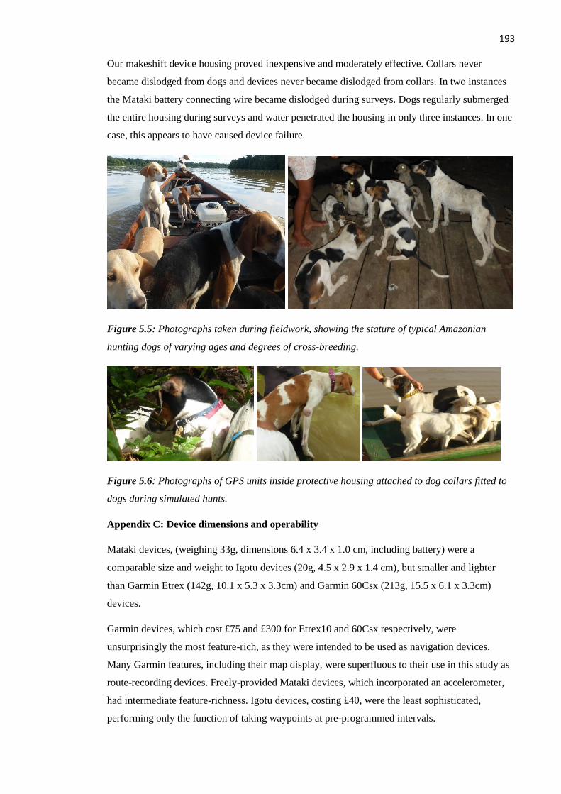
193 Our makeshift device housing proved inexpensive and moderately effective. Collars never

became dislodged from dogs and devices never became dislodged from collars. In two instances

the Mataki battery connecting wire became dislodged during surveys. Dogs regularly submerged

the entire housing during surveys and water penetrated the housing in only three instances. In one

case, this appears to have caused device failure.

Figure 5.5: Photographs taken during fieldwork, showing the stature of typical Amazonian

hunting dogs of varying ages and degrees of cross-breeding.

Figure 5.6: Photographs of GPS units inside protective housing attached to dog collars fitted to

dogs during simulated hunts.

Appendix C: Device dimensions and operability

Mataki devices, (weighing 33g, dimensions 6.4 x 3.4 x 1.0 cm, including battery) were a

comparable size and weight to Igotu devices (20g, 4.5 x 2.9 x 1.4 cm), but smaller and lighter

than Garmin Etrex (142g, 10.1 x 5.3 x 3.3cm) and Garmin 60Csx (213g, 15.5 x 6.1 x 3.3cm)

devices.

Garmin devices, which cost £75 and £300 for Etrex10 and 60Csx respectively, were

unsurprisingly the most feature-rich, as they were intended to be used as navigation devices.

Many Garmin features, including their map display, were superfluous to their use in this study as

route-recording devices. Freely-provided Mataki devices, which incorporated an accelerometer,

had intermediate feature-richness. Igotu devices, costing £40, were the least sophisticated,

performing only the function of taking waypoints at pre-programmed intervals.

194 Garmin devices use conventional AA batteries. We were able to purchase such batteries even in

remote Amazonian towns. Garmin devices also featured a graphical menu interface, which

permitted operation and device programming when away from a computer and freely available

software (Garmin Basemap) to enable the download and processing of data. Igotu devices feature

a dedicated USB charging cable, single-button operation, easily interpretable LED status

indicators and free software (@trip) for device programming and data processing. These

characteristics meant that Garmin and Igotu devices could be powered and programmed when in

the field, and the data they recorded could be downloaded without any specialist equipment or

training. Mataki batteries required custom-made adaptors in order to be recharged via USB. Data

uploading and device programming was achieved using straightforward code when attached to a

computer via a base-station. Despite the provision by Mataki of user guides and training material,

MIA found that device LEDs did not intuitively indicate device settings or problems when in use,

making the diagnoses of mechanical errors challenging in the field. Mataki devices thus required

specialist, custom-made hardware and training in order to be used.

195

Chapter 6: Concluding Remarks

196

6.1 The need for nuance

The conclusions of this thesis are broadly congruent with the conservationist critique of large-

scale inappropriate infrastructural development and perverse government subsidies for

colonisation and deforestation (Laurance et al., 2004), but diverge somewhat from the largely

polarised existing literature regarding community extractivist use of tropical forest resources

(Brandon et al., 1998; Schwartzman et al., 2000). Echoing the results of numerous existing

studies, we found that at the regional scale, much of the anthropogenic disturbance evident in

rural areas, is in fact driven or directly caused by non-rural, non-local factors and agents including

urban centres (DeFries et al., 2010), colonisation policies (Peres and Schneider, 2012) and

(especially transport) infrastructure (Peres, 2001). The depletion of game fauna was also found to

be an urban-driven phenomenon (Bowen‐Jones and Pendry, 1999). Cognisant of the hypocrisy of

inveighing against infrastructural development in tropical regions, whose inhabitants deserve the

improved standards of living these may afford, we agree with authors who advocate for a well-

planned balance between infrastructure and environmental protection, which will bring the

greatest possible net social benefits, with the lowest associated ecological costs (Margules and

Pressey, 2000; Caro et al., 2014; Laurance et al., 2015).

By contrast, we find that much of the debate surrounding the extractive use of tropical forests,

and surrounding hunting in particular, presents a needless false dichotomy between what may

(exaggeratedly) be termed anthropophobic and anthropophilic approaches to conservation

(although several authors have attempted to bridge these divides, for example Peres and

Zimmerman (2001)). Our results suggest that a more nuanced attitude towards extractive

communities is needed. In our study regions, we found that forest-dependent communities clearly

do impact forest fauna, but equally that they do not eradicate it. The question “Do forest-

dependent communities extirpate terrestrial game fauna?” should be replaced with “under what

social, demographic, technological and ecological conditions, and to what degree, do forest-

dependent communities cause net species-specific and assemblage-wide depletion of terrestrial

game fauna, relative to a baseline of the absence of those communities?”. This explicitly

recognises that the presence of those communities may deter the still-greater ecological impacts

of non-local agents. These approaches are becoming increasingly common, for example through

the use of bio-demographic and bio-economic models (Damania et al., 2005; Levi, et al., 2011).

In the remaining section of this thesis, I briefly summarise the main findings of the four data

chapters (this section will be largely without references as I am summarising the findings of this

study), draw out a recurrent theme, present potential conservation strategies and indicate fruitful

areas of future research.

197

6.2 Summary of key findings

In Chapter 2, we found that at the regional scale, urban centres, fluvial accessibility and terrestrial

transport infrastructure drive different patterns of anthropogenic disturbance along cul-de-sac

Amazonian rivers both directly and indirectly, by influencing rural population density. Non-

fluvial transport infrastructure, for example roads, transformed colonisation and land-use patterns

in otherwise inaccessible rivers. Even our conservative characterisation of hunting catchment

areas, non-structural disturbance affected an area over 18 times larger than structural disturbance.

In Chapter 3, semi-subsistence agriculturalists in the Jurua region were found to bear a triple

burden imposed by the ecosystem disservices of terrestrial vertebrate crop raiders including; (a)

5.5% direct annual losses to crop raiders; (b) the labour and opportunity costs required to protect

agricultural plots against crop raiders and avoid estimated losses that would be an order of

magnitude higher; and (c) reduced opportunities to plant more palatable manioc varieties. As

agricultural production is the primary livelihood and hunting is deemed less significant, the

potential gains of hunting crop raiders do not fully compensate crop losses. Households in more

isolated areas, that are already socially disadvantaged, are precisely those suffering higher losses

to crop raiders.

In Chapter 4, we found that evidence for the depletion of terrestrial vertebrates in proximity to

semi-subsistence communities in the Juruá and Uatumã regions was mixed. Only a select few

species, especially large-bodied, group-living species, were heavily depleted by communities.

Although species-specific shifts in activity patterns in response to community settlements were

not evident, diurnal species were less prevalent near to communities. Collared peccaries may be

competitively released in the absence of white lipped peccaries. Urban centres exerted a

landscape-scale impact, depressing the aggregate biomass of forest vertebrates. Areas close to

perennial streams were especially vulnerable to hunting. Our evidence for hunting-mediated

depletion is likely to (a) be conservative due to our sampling strategy, which runs against the

landscape scale gradient of primary productivity, and (b) represents a “best case scenario”, due to

the high local availability of alternative animal protein, which effectively protects game stocks by

reducing hunting pressure in our study regions (Endo et al., 2016).

In Chapter 5, open source Mataki devices were found to be of intermediate reliability and

accuracy when used to characterise the spatial behaviour of hunting dogs and their masters during

simulated hunts. Hunting dogs travelled only ~ 13% farther than their masters, which was less

than anticipated. There is evidence that hunters based in urban centers travel significantly farther

than rural hunters. Local attitudes towards hunting dogs were mixed; they were recognised to

have deleterious impacts on wildlife, but were commonly used to defend against crop raiders.

198

6.3 Urban influence

A recurring theme throughout this thesis, has been the pivotal role played by urban centres both in

the livelihoods of rural Amazonians and in the anthropogenic disturbance of forest biodiversity, at

the regional, landscape and household scales (Pinedo-Vásquez and Padoch, 2009).

Regionally, urban centres were found to be a strong driver of whole-river rural population

density. This is unsurprising given the economic, information, and social services centrality of

urban centres in the lives of even remote ribeirinho households (Parry et al., 2010). These

households are themselves an important driver of both structural and non-structural forest

disturbance. Our analysis of anthropogenic disturbance in proximity to cul-de-sac rivers likely

underestimates the impacts of urbanites, who are more financially able to make long-distance

forays into river headwaters to extract NTFPs, especially forest game vertebrates. The impact of

commercial hunters has been shown to be more devastating than that of subsistence hunters

(Vega et al., 2013). Assuming relatively secure tenure and moderate discount rates, long-term

subsistence local resource users are theoretically incentivised to conserve natural capital such as

game or timber stocks, in order to continually benefit from the harvestable “interest” (Godoy et

al., 2001). Urban commercial hunters, loggers and gold miners, however, who are not dependent

upon the persistence of viable resource stocks in a particular location and who have alternative

livelihoods, benefit from liquidating natural capital as efficiently as possible.

At the landscape scale, urban centres, rather than rural communities, were found to depress the

aggregate biomass of both crop raiding and hunted species. This reinforces the notion that

household location choice is a livelihood trade-off, in this case, between greater access to natural

resources and greater access to market goods and services (Alonso, 1964). Urban or suburban

households incur lower losses of their staple crops to vertebrate crop raiders, and therefore benefit

from higher yields, lower labour input in guarding activities, and the opportunity to plant less

chemically defended, more palatable varieties of manioc. However, as suggested by (a) the lower

biomass of hunted vertebrates near towns; (b) the longer distances travelled by urbanites during

simulated hunts; and (c) evidence that hunter catch-per-unit effort is negatively related to urban

proximity (Endo et al., 2016), urbanites can less readily access terrestrial game meat. The

continuing rural exodus in Amazonia, as well as our finding that rural population density is

strongly influenced by access to urban centres, are testament to the fact that in the livelihood

calculations made by the majority of ribeirinhos, the costs of losing access to plentiful natural

resources are outweighed by the benefits of closer integration into markets and better access to

goods and services. This household level decision-making process is in fact universal to the wider

urban-to-rural-to-wilderness gradient worldwide, but particularly in tropical countries, thereby

shaping many of the conservation and development challenges of contemporary times (Browder.,

2002).

199 Brazil is currently facing a deep political crisis and related economic uncertainty. Even before the

corruption scandals and economic slowdown that ejected the former President from public office,

however, Brazil was already facing a crisis of environmental identity (Loyola, 2014). Many

Brazilian progressive environmental policies are being undermined (Ferreira et al., 2014), and

there have been continued legal calls to compromise the status of existing protected areas (de

Marques. and Peres, 2015). Funding for environmental agencies has been substantially reduced

and the much lauded federal Forest Code that requires a legal limit to deforestation on private

properties has been watered down (Soares-Filho et al., 2014). Destructive infrastructure projects

including the controversial Belo Monte dam and long distance road network expansion are

ongoing (Laurance et al., 2001). These economic and political factors seem likely to result in both

a further weakening of environmental legislation and enforcement (Campos-Silva et al., 2015, as

well as a reduction in the extent of government welfare support.

These trends will likely strengthen the aforementioned influence of urban centres. Government

welfare support, both through direct payments such as the Bolsa Familia, which our interview

respondents identified as an important livelihood component, and through the provision of

services such as digital classrooms in rural communities, have until now slowed the rate of rural

abandonment and increased the rate of sedentarism. If this support is significantly diminished,

then the rapidly growing rural population is likely to continue to urbanise. Although the direct

pressures exerted by rural households is likely to decrease and land abandonment may result in

forest regrowth, weaker environmental legislation and lower funding will further reduce the

defensibility of protected areas, which are already chronically underfunded and under-staffed.

200

6.4 Conservation Strategies

In light of the aforementioned findings, what conservation measures could be taken to ameliorate

biodiversity losses? Our study appears to have identified some “low-hanging fruits” which are

promising conservation strategies.

At the regional level, our analysis of cul-de-sac rivers suggests that conservationists should

continue to oppose expensive and ill-conceived mega-infrastructure projects and perverse

subsidies, particularly in low-governance frontiers lacking land-use planning. Given the need for

the Brazilian government to demonstrate judicious spending of tax revenue, uneconomic

subsidies including the agricultural resettlement program which has driven unsustainable and

unprofitable agricultural expansion at the expense of tropical forests (Peres and Schneider, 2012),

should be opposed. Realistic cost-benefit analyses for infrastructure development including road-

building, are as much a civic duty as an environmental imperative (Caro et al., 2014; Laurance et

al., 2014; Laurance et al., 2015). The suboptimal placement of the Balbina reservoir, for example

has wrought large-scale ecological damage despite modest energy generation (Fearnside, 1989;

Benchimol and Peres, 2015), yet an expansionist hydroelectric development strategy for all steep

gradient river basins of Brazilian Amazonia remains largely unopposed (Lees et al., 2016).

In the Neotropics, terrestrial vertebrate crop raiding species are generally disturbance-tolerant and

of relatively low conservation concern (Parry et al., 2009), whereas large primates including

woolly and spider monkeys are both extremely vulnerable to depletion via hunting offtake (Peres,

1990) and are not identified as problematic species. Furthermore, many ribeirinho communities

are disinclined to hunt primates for cultural reasons (Mittermeier, 1987). This suggests that

placing stronger legal restrictions on the hunting of the most harvest sensitive species whilst

simultaneously loosening restrictions on the hunting of crop raiding species, would minimally

impact local livelihoods whilst benefitting biodiversity. This strategy would likely be less

successful in indigenous reserves where the hunting of primates is culturally important (Da Silva

et al., 2005). Similarly, this strategy is not easily applicable in the Afrotropics, where endangered

elephants and chimpanzees are also both problematic crop raiders and frequently cause injury and

endanger human life (Thirgood et al., 2005).

A related strategy would be to simultaneously place stronger restrictions on the use of specially

bred hunting dogs, whilst tolerating or encouraging the use of other domestic dogs. The benefits

that domestic dogs bring to local communities in warding away dangerous large felids and

chasing away crop raiders, should be recognised (Verdade et al., 2004), but equally these benefits

can accrue without the ecological damage potentially wrought by bred hunting dogs.

Given the importance of fluvial accessibility to hunters, one conservation strategy may be to

empower communities sited at the mouths of perennial streams (igarapés) to restrict the access of

non-resident hunters. The success of this strategy would be highly region-specific however.

201 Hunting in the Juruá region, for example, often occurs when water levels are high and returns

from fishing are poor (Endo et al., 2016). This is precisely the period when igarapés can easily be

bypassed by travelling through the flooded várzea.

Conservationists must question whether active terrestrial game management in rural Amazonia is

necessary, desirable, or even possible. The evidence from this thesis is not sufficient to conclude

that rural communities are emptying the surrounding forests of terrestrial game vertebrates,

though they are impacting large, vulnerable and ecologically important species. Adaptive

management of game stocks would require both robust faunal monitoring and representative

unhunted baseline sites to serve as a basis for comparison (Walters, 1986). These measures would

be costly and administratively challenging, but beneficial in themselves in that they would

potentially create wildlife refugia and actively engage local communities in the process of

conservation. Radical new conservation programs may be less effective than reinvigorating

existing interventions including ProBUC faunal monitoring, which have proven successful, but

are underfunded (Ferraz et al., 2008).

As noted, terrestrial game species are harder to monitor and restrict access to than pirarucu in

oxbow lakes or turtles on beaches, and their lower productivity entails that communities are

unlikely to observe a direct and rapid benefit from protection. These difficulties and the fact that

the availability of aquatic protein has apparently reduced the hunting pressure in our study

regions, and may be responsible for relatively low wildmeat extraction rates in the Amazon basin

(Fa et al., 2002), suggest that an indirect and holistic strategy holds more promise. Hunting does

not occur in isolation, but is part of a complex web of livelihood activities (Coomes et al., 2004).

The most effective means of protecting terrestrial game stocks, may in fact be to continue to focus

on the sustainability of local fisheries. The limited resources available to conservationists may be

best spent combatting illegal logging, gold mining and perverse commercial fishing practices

such as discarding of low-value species (Ruffino, 2001). These practices create negative

externalities felt by local communities (Biller, 1994), as they depress fish stocks, thereby driving

unsustainable hunting.

Lastly, and on a related note, conservationists may need to focus more attention on the

unsustainable practices of Amazonian urbanites who are shown in this thesis and in other studies,

to be having a large impact on biodiversity (DeFries, 2010). Environmental education and

enforcement are likely to be better per-capita value for money in urban areas due to their high

population density. Amazonian rural population densities in many areas are currently generally

well below the 1 person/km2 level generally deemed to enable relatively sustainable subsistence

hunting (Robinson and Bennett, 2013), therefore our current focus on rural communities may be

misplaced.

202

6.5 Future Research

Throughout this thesis, numerous intriguing avenues were identified that it was not possible to

fully pursue. Analyses of region-wide riverine disturbance could be strengthened by comparing

patterns of anthropogenic disturbance across a wider spectrum of rivers, ranging from virtually

uninhabited, to cul-de-sac, to road-intersected, and finally to a bead-chain pattern. Levels of

anthropogenic disturbance are likely to vary far more strongly between these categories than

within them and this would provide a clearer picture of the likely current trajectory of virtually

undisturbed rivers. This would require a clear analytic framework in order to apportion data

between rivers and a hydrological river-basin approach may be promising in this respect.

Similarly, if historical demographic data were available, one could analyse the human-mediated

evolution of disturbance along a set of rivers. Given the structured nature of the causal

interactions in this system, a path analysis using a larger sample size may be preferable to GLMs.

Lastly, studies of anthropogenic disturbance tend to either focus on large-scale demographic

processes without distinguishing cultural differences (Laurance et al., 2002) or focus closely on

the decision-making of a spatially restricted population sample (Pichón, 1997). If the spatial

distribution of different cultural groups were known, then their different impacts could be

compared (see dos Santos Silva et al. (2008) for a case study using remote-sensing image-mining

to identify agents of deforestation).

During interviews with semi-subsistence agriculturalists concerning terrestrial vertebrate crop

raiding many interactions between human livelihoods and both terrestrial and aquatic species,

were touched upon, but could not be pursued. Crop protection and human-wildlife conflict

mitigation strategies have been extensively studied in the Afrotropics (Nelson et al., 2003), where

conflict with dangerous, but endangered megafauna is common. The fact that Amazonian crop

raiders are smaller-bodied than their Palaeotropical counterparts, and generally neither very

dangerous nor highly endangered, may explain why they have been less studied. Human-wildlife

conflict mitigation strategies in the Neotropics are however important to study, partly because

rural Amazonians are frequently attacked and killed by large felids, crocodilians and serpents

(Neto et al., 2011), their fisheries are impacted by aquatic predators including river dolphins and

giant otters (Rosas‐Ribeiro et al., 2012), and their livestock is predated by felids, mustelids,

eagles, and snakes (Silveira et al., 2008). It is also important because these conflicts often result

in retaliatory killings of threatened species (Marchini, 2012). For these reasons, more detailed

research should be conducted into the nature and effectiveness of strategies used by Amazonians

to protect themselves and their livelihoods. In particular, in-depth assessments of the use of both

hunting and domestic dogs should be made in order to fully elucidate both their importance and

the damage they cause to tropical forest biodiversity.

203

6.5 References

Alonso, W., 1964. Location and land use. Toward a general theory of land

rent. Cambridge, Mass. Harvard University Press

Benchimol, M. and Peres, C.A., 2015. Widespread forest vertebrate extinctions induced

by a mega hydroelectric dam in lowland Amazonia. PloS One, 10(7), p.e0129818.

Biller, D., 1994. Informal gold mining and mercury pollution in Brazil (Vol. 1304).

World Bank Publications.

Bowen‐Jones, E. and Pendry, S., 1999. The threat to primates and other mammals from

the bushmeat trade in Africa, and how this threat could be diminished 1. Oryx, 33(3), pp.233-246.

Brandon, K., Redford, K.H. and Sanderson, S.E. eds., 1998. Parks in peril: people,

politics, and protected areas (No. 333.783 P252). Washington, DC: Island Press.

Browder, J.O., 2002. The urban-rural interface: Urbanization and tropical forest cover

change. Urban Ecosystems, 6(1-2), pp.21-41.

Campos-Silva, J.V., da Fonseca Junior, S.F. and Peres, C.A., 2015. Policy reversals do

not bode well for conservation in Brazilian Amazonia. Natureza & Conservação, 13(2), pp.193-

195.

Caro, T., Dobson, A., Marshall, A.J. and Peres, C.A., 2014. Compromise solutions

between conservation and road building in the tropics. Current Biology, 24(16), pp.R722-R725.

Coomes, O.T., Barham, B.L. and Takasaki, Y., 2004. Targeting conservation–

development initiatives in tropical forests: insights from analyses of rain forest use and economic

reliance among Amazonian peasants. Ecological Economics, 51(1), pp.47-64.

Damania, R., Milner-Gulland, E.J. and Crookes, D.J., 2005. A bioeconomic analysis of

bushmeat hunting. Proceedings of the Royal Society of London B: Biological

Sciences, 272(1560), pp.259-266.

Da Silva, M.N., Shepard Jr, G.H. and Yu, D.W., 2005. Conservation implications of

primate hunting practices among the Matsigenka of Manu National Park. Neotropical

Primates, 13(2), pp.31-36.

de Marques, A.A.B. and Peres, C.A., 2015. Pervasive legal threats to protected areas in

Brazil. Oryx, 49(01), pp.25-29.

DeFries, R.S., Rudel, T., Uriarte, M. and Hansen, M., 2010. Deforestation driven by

urban population growth and agricultural trade in the twenty-first century. Nature

Geoscience, 3(3), pp.178-181.

204

dos Santos Silva, M.P., Camara, G., Escada, M.I.S. and de Souza, R.C.M., 2008. Remote‐

sensing image mining: detecting agents of land‐use change in tropical forest areas. International

Journal of Remote Sensing, 29(16), pp.4803-4822.

Endo, W., Peres, C.A. and Haugaasen, T., 2016. Flood pulse dynamics affects

exploitation of both aquatic and terrestrial prey by Amazonian floodplain settlements. Biological

Conservation, 201, pp.129-136.

Fa, J.E., Peres, C.A. and Meeuwig, J., 2002. Bushmeat exploitation in tropical forests: an

intercontinental comparison. Conservation Biology, 16(1), pp.232-237.

Fearnside, P.M., 1989. Brazil's Balbina Dam: Environment versus the legacy of the

pharaohs in Amazonia. Environmental Management, 13(4), pp.401-423.

Ferraz, G., Marinelli, C.E. and Lovejoy, T.E., 2008. Biological monitoring in the

Amazon: recent progress and future needs. Biotropica, 40(1), pp.7-10.

Ferreira, J., Aragão, L.E.O.C., Barlow, J., Barreto, P., Berenguer, E., Bustamante, M.,

Gardner, T.A., Lees, A.C., Lima, A., Louzada, J. and Pardini, R., 2014. Brazil's environmental

leadership at risk. Science, 346(6210), pp.706-707.

Godoy, R., Kirby, K. and Wilkie, D., 2001. Tenure security, private time preference, and

use of natural resources among lowland Bolivian Amerindians. Ecological Economics, 38(1),

pp.105-118.

Laurance, W.F., Cochrane, M.A., Bergen, S., Fearnside, P.M., Delamônica, P., Barber,

C., D'Angelo, S. and Fernandes, T., 2001. The future of the Brazilian

Amazon. Science, 291(5503), pp.438-439.

Laurance, W.F., Albernaz, A.K., Schroth, G., Fearnside, P.M., Bergen, S., Venticinque,

E.M. and Da Costa, C., 2002. Predictors of deforestation in the Brazilian Amazon. Journal of

Biogeography, 29(5‐6), pp.737-748.

Laurance, W.F., Albernaz, A.K., Fearnside, P.M., Vasconcelos, H.L. and Ferreira, L.V.,

2004. Deforestation in Amazonia. Science, 304(5674), pp.1109-1111.

Laurance, W.F., Clements, G.R., Sloan, S., O’Connell, C.S., Mueller, N.D., Goosem, M.,

Venter, O., Edwards, D.P., Phalan, B., Balmford, A. and Van Der Ree, R., 2014. A global

strategy for road building. Nature, 513(7517), pp.229-232.

Laurance, W.F., Peletier-Jellema, A., Geenen, B., Koster, H., Verweij, P., Van Dijck, P.,

Lovejoy, T.E., Schleicher, J. and Van Kuijk, M., 2015. Reducing the global environmental

impacts of rapid infrastructure expansion. Current Biology, 25(7), pp.R259-R262.

205

Lees, A.C., Peres, C.A., Fearnside, P.M., Schneider, M. and Zuanon, J.A., 2016.

Hydropower and the future of Amazonian biodiversity. Biodiversity and Conservation, 25(3),

pp.451-466.

Levi, T., Shepard, G.H., Ohl-Schacherer, J., Wilmers, C.C., Peres, C.A. and Yu, D.W.,

2011. Spatial tools for modeling the sustainability of subsistence hunting in tropical

forests. Ecological Applications, 21(5), pp.1802-1818.

Loyola, R., 2014. Brazil cannot risk its environmental leadership. Diversity and

Distributions, 20(12), pp.1365-1367.

Marchini, S. and Macdonald, D.W., 2012. Predicting ranchers’ intention to kill jaguars:

case studies in Amazonia and Pantanal. Biological Conservation, 147(1), pp.213-221.

Margules, C.R. and Pressey, R.L., 2000. Systematic conservation planning.

Nature, 405(6783), pp.243-253.

Mittermeier, R.A., 1987. Effects of hunting on rain forest primates. in C. Marsch, R.A.

Mittermeier (Eds.), Primate Conservation in the Tropical Rain Forest, Alan R. Liss, New York

(1987), pp. 109–146

Nelson, A., Bidwell, P. and Sillero-Zubiri, C., 2003. A review of human-elephant conflict

management strategies. People & Wildlife, A Wildlife Conservation Research Unit, Born Free

Foundation Partnership.

Neto, M.F.C., Neto, D.G. and Haddad, V., 2011. Attacks by jaguars (Panthera onca) on

humans in Central Brazil: report of three cases, with observation of a death. Wilderness &

Environmental Medicine, 22(2), pp.130-135

Parry, L., Barlow, J. and Peres, C.A., 2009. Allocation of hunting effort by Amazonian

smallholders: implications for conserving wildlife in mixed-use landscapes. Biological

Conservation, 142(8), pp.1777-1786.

Parry, L., Day, B., Amaral, S. and Peres, C.A., 2010. Drivers of rural exodus from

Amazonian headwaters. Population and Environment, 32(2-3), pp.137-176.

Peres, C.A., 1990. Effects of hunting on western Amazonian primate

communities. Biological Conservation, 54(1), pp.47-59.

Peres, C.A., 2001. Paving the way to the future of Amazonia. Trends in Ecology &

Evolution, 16(5), pp.217-219.

Peres, C.A. and Zimmerman, B., 2001. Perils in parks or parks in peril? Reconciling

conservation in Amazonian reserves with and without use. Conservation Biology, 15(3), pp.793-

797.

206

Peres, C.A. and Schneider, M., 2012. Subsidized agricultural resettlements as drivers of

tropical deforestation. Biological Conservation, 151(1), pp.65-68.

Pichón, F.J., 1997. Colonist land‐allocation decisions, land use, and deforestation in the

Ecuadorian Amazon frontier. Economic Development and Cultural Change, 45(4), pp.707-744.

Pinedo-Vásquez, M. and Padoch, C., 2009. Urban and rural and in-between: Multi-sited

households, mobility and resource management in the Amazon floodplain. Mobility and

migration in indigenous Amazonia: Contemporary Ethnoecological Perspectives, 11, pp.86-96.

Robinson, J.G. and Bennett, E.L., 2013. Hunting for sustainability in tropical forests.

Columbia University Press.

Rosas‐Ribeiro, P.F., Rosas, F.C. and Zuanon, J., 2012. Conflict between fishermen and

giant otters Pteronura brasiliensis in Western Brazilian Amazon. Biotropica, 44(3), pp.437-444.

Ruffino, M.L., 2001. Strategies for managing biodiversity in Amazonian fisheries. The

Brazilian Environmental and Renewable Natural Resources Institute- IBAMA

Schwartzman, S., Moreira, A. and Nepstad, D., 2000. Rethinking tropical forest

conservation: perils in parks. Conservation Biology, 14(5), pp.1351-1357.

Silveira, L., Boulhosa, R., Astete, S. and Jácomo, A.A., 2008. Management of domestic

livestock predation by jaguars in Brazil. Cat News, 4, pp.26-30.

Soares-Filho, B., Rajão, R., Macedo, M., Carneiro, A., Costa, W., Coe, M., Rodrigues, H.

and Alencar, A., 2014. Cracking Brazil's forest code. Science, 344(6182), pp.363-364.

Thirgood, S., Woodroffe, R. and Rabinowitz, A., 2005. The impact of human-wildlife

conflict on human lives and livelihoods. Conservation Biology Series-Cambridge, 9, p.13.

VEGA, M.G., Carpinetti, B., Duarte, J. and Fa, J.E., 2013. Contrasts in livelihoods and

protein intake between commercial and subsistence bushmeat hunters in two villages on Bioko

Island, Equatorial Guinea. Conservation Biology, 27(3), pp.576-587.

Verdade, L.M. and Campos, C.B., 2004. How much is a puma worth?: economic

compensation as an alternative for the conflict between wildlife conservation and livestock

production in Brazil. Biota Neotropica, 4(2), pp.1-4.

Walters, C., 1986. Adaptive Management of Renewable Resources. Macmillan, New

York.